Probability & Statistics 2 · ⁨הסתברות וסטטיסטיקה 2⁩

The Poisson distribution 泊松分布 $X \sim \mathrm{Po}(\lambda)$ models the number of random events in a fixed interval, when events happen at a steady average rate $\lambda$:

For a Poisson variable the mean and the variance are both equal to $\lambda$. The Poisson distribution is a good approximation 近似 to the binomial distribution when $n$ is large and $p$ is small. The normal distribution (with continuity correction) approximates the Poisson when $\lambda$ is large.

Worked example. $X \sim \mathrm{Po}(3)$. Find $P(X = 2)$.

When you change a variable by a linear rule, the expectation 期望 (mean) and variance 方差 follow these rules:

For two independent variables $X$ and $Y$: Two useful facts: if $X$ has a normal distribution 正态分布 then so does $aX + b$; and the sum of independent Poisson variables is again Poisson.

Worked example. $X$ has mean $5$ and variance $4$. Find $E(3X - 1)$ and $\mathrm{Var}(3X - 1)$.

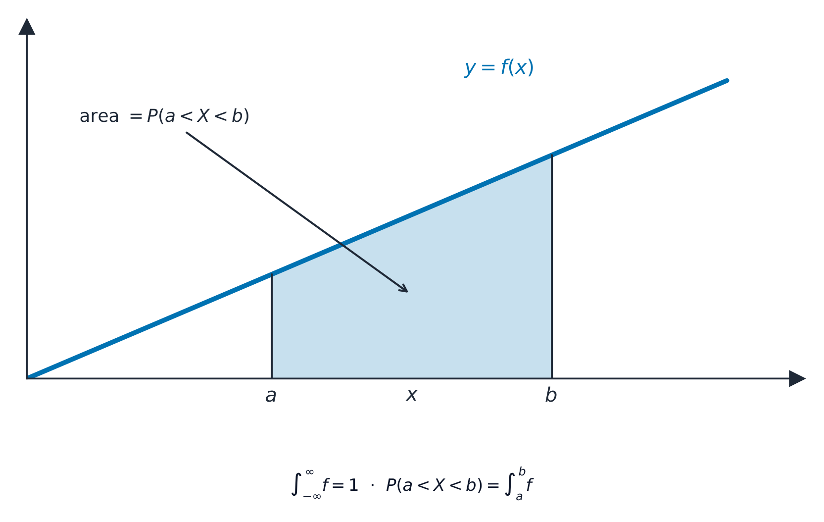
A continuous random variable 连续型随机变量 can take any value in a range. Its probabilities come from a probability density function 概率密度函数 $f(x)$, with two key properties:

A probability is the area under $f$, and the mean is found by integration:

The cumulative distribution function 累积分布函数 is $F(x) = P(X \leqslant x) = \int_{-\infty}^{x} f(t)\,dt$; the median 中位数 solves $F(m) = 0.5$, and other percentiles 百分位数 solve $F(x) = p$.

Worked example. A continuous variable has $f(x) = \tfrac12 x$ for $0 \leqslant x \leqslant 2$ (and $0$ elsewhere). Find $E(X)$.

The variance uses the same idea, $\mathrm{Var}(X)=\displaystyle\int_{-\infty}^{\infty}x^2 f(x)\,dx-\big(E(X)\big)^2$. For the same $f(x)=\tfrac12 x$ on $[0,2]$: $\displaystyle\int_0^2 x^2\cdot\tfrac12 x\,dx=\left[\tfrac{x^4}{8}\right]_0^2=2$, so $\mathrm{Var}(X)=2-\left(\tfrac43\right)^2=2-\tfrac{16}{9}=\tfrac{2}{9}$.

A sample 样本 is a small group chosen from the whole population 总体. A random sample needs randomness 随机性, so that every member has a fair chance of being chosen.

Some methods are unsatisfactory because they are biased 有偏: sampling only volunteers, or the first 20 people to arrive, over-represents certain kinds of people. A genuinely random sample uses random numbers – number every member of the population, then draw numbers (from a table or a generator) to decide who is in the sample.

The sample mean $\bar{X}$ is itself a random variable, with

By the Central Limit Theorem 中心极限定理, for a large sample $\bar{X}$ is approximately normal, whatever the shape of the population.

From a sample you can find unbiased estimates 无偏估计 of the population mean and variance. A confidence interval 置信区间 gives a range that probably contains the true mean. When the population is normal with known $\sigma$ (or the sample is large), a $95\%$ interval is

You can also find a confidence interval for a population proportion 总体比例 from a large sample.

Worked example. A sample of $n = 64$ has mean $\bar{x} = 50$, from a population with $\sigma = 8$. Find a $95\%$ confidence interval for the population mean.

A hypothesis test 假设检验 uses sample data to judge a claim. You set up two statements: the null hypothesis 原假设 $H_0$ (the claim being tested, usually "no change") and the alternative hypothesis 备择假设 $H_1$ (what you suspect instead). The test is one-tailed 单尾 if $H_1$ points one way (e.g. $\mu > 50$) and two-tailed 双尾 if it allows both ways ($\mu \neq 50$).

You fix a significance level 显著性水平 (often $5\%$), work out a test statistic 检验统计量 from the data, and see whether it lands in the rejection region 拒绝域 (also called the critical region); if it does you reject $H_0$, otherwise the statistic is in the acceptance region.

Two mistakes are possible: a Type I error 第一类错误 is rejecting $H_0$ when it is actually true; a Type II error 第二类错误 is accepting $H_0$ when it is actually false. You can find their probabilities from the rejection region: $P(\text{Type I})=P(\text{statistic in the rejection region}\mid H_0)$ – this equals the significance level – and $P(\text{Type II})=P(\text{statistic in the acceptance region}\mid H_1$ true for a stated value$)$, computed from the binomial, Poisson, or normal distribution.

Worked example. A population is claimed to have mean $50$, with $\sigma = 8$. A sample of $n = 64$ gives $\bar{x} = 52$. Test at the $5\%$ level whether the mean has changed.

$H_0\!: \mu = 50$ and $H_1\!: \mu \neq 50$ (two-tailed). The test statistic is

The critical value at $5\%$ (two-tailed) is $1.96$. Since $2 > 1.96$, you reject $H_0$: there is evidence the mean has changed.

Worked example (a binomial test). A coin is claimed fair but suspected of landing heads too rarely: $H_0\!:p=0.5$, $H_1\!:p<0.5$. In $n=30$ tosses you see $X=9$ heads. Under $H_0$, $X\sim B(30,0.5)$, so the one-tailed tail probability is

Since $0.021<0.05$, reject $H_0$: the coin does seem biased against heads. (For large $n$ the binomial is approximated by a normal; a Poisson test works the same way for rare events. And here, if the rule is "reject when $X\leqslant 9$", then $P(\text{Type I})=P(X\leqslant 9\mid p=0.5)\approx0.021$.)

• Use the Poisson distribution for rare, random, independent events; its mean equals its variance ($= \lambda$).
• When combining independent random variables, variances add (they never subtract).
• For a hypothesis test, state $H_0$ and $H_1$, the significance level, the test statistic, and a conclusion in context.
• For a confidence interval, use the correct $z$ (or $t$) value and interpret it in words.