Probability & Statistics 1

Choose a diagram that suits the data. You should be able to draw and read:

• a stem-and-leaf diagram 茎叶图 (keeps the original values and shows the shape);
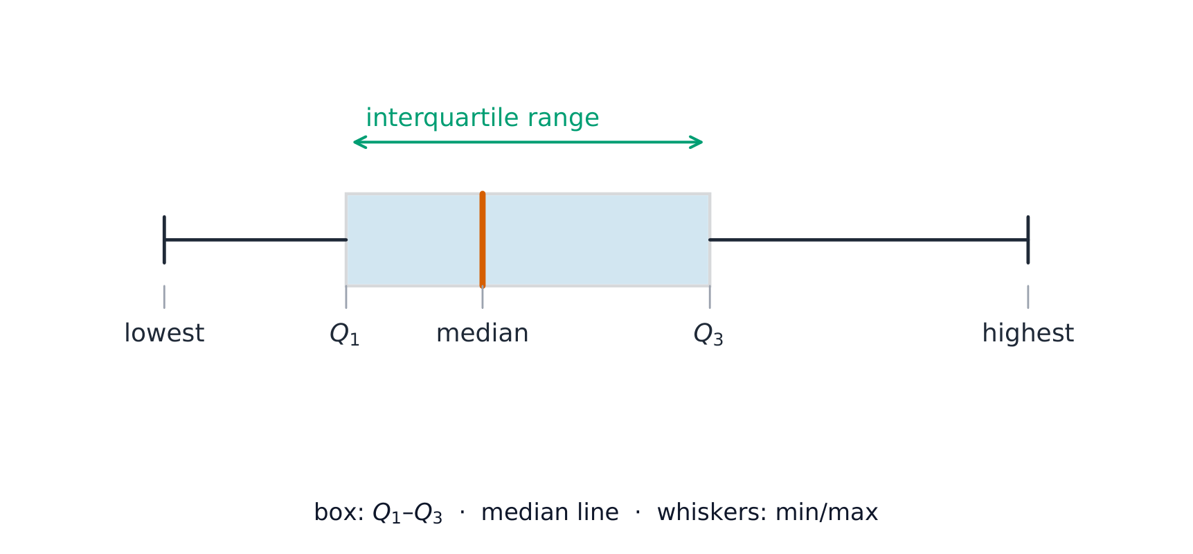
• a box-and-whisker plot 箱线图 (shows the lowest value, the three quartiles, and the highest value);
• a histogram 直方图 (for grouped data, where the area of each bar shows the frequency);
• a cumulative frequency 累积频数 graph (running totals, used to estimate the median and quartiles).

A cumulative frequency curve is S-shaped; read the median across from half the total frequency, and the quartiles from one and three quarters

The box spans the quartiles $Q_1$ to $Q_3$; the whiskers reach the lowest and highest values.

Averages and spread

A measure of central tendency 集中趋势 is a single "middle" value:

• the mean 平均数 $\bar{x} = \dfrac{\sum x}{n}$ (the average);
• the median 中位数 (the middle value when the data is in order);
• the mode 众数 (the most common value).

A measure of variation 离散程度 shows how spread out the data is:

• the range (of data) 极差 (highest $-$ lowest);
• the interquartile range 四分位距 (upper quartile $-$ lower quartile);
• the standard deviation 标准差 $\sigma = \sqrt{\dfrac{\sum x^2}{n} - \bar{x}^2}$.

You often work from the totals $\sum x$ and $\sum x^2$. The square of the standard deviation is the variance 方差.

Worked example. For $10$ values, $\sum x = 50$ and $\sum x^2 = 300$. Find the mean and standard deviation.

A permutation 排列 is an arrangement where order matters; a combination 组合 is a selection where order does not matter. The numbers are

To arrange objects in a line when some are repeated, divide by the factorial of each repeat count.

Order matters for a permutation, but not for a combination

Worked example. How many different arrangements are there of the letters of the word NEEDLESS?

There are $8$ letters, with E repeated $3$ times and S repeated $2$ times:

Dice: a familiar starting point for probability.

Find a probability by counting equally likely outcomes, or by using permutations and combinations. Combine probabilities with these rules:

• addition for "or": $P(A \cup B) = P(A) + P(B) - P(A \cap B)$;
• multiplication for "and" when events are independent: $P(A \cap B) = P(A)\,P(B)$.

The overlap of the two circles is $A\cap B$; the addition rule subtracts it once so it is not counted twice.

Two events are mutually exclusive events 互斥事件 if they cannot both happen, and independent events 独立事件 if one happening does not change the chance of the other. To test independence, check whether $P(A \cap B) = P(A)\times P(B)$. A conditional probability 条件概率 is the chance of $A$ given that $B$ has happened: $P(A \mid B) = \dfrac{P(A \cap B)}{P(B)}$.

Worked example. Events have $P(A) = 0.5$, $P(B) = 0.4$ and $P(A \cap B) = 0.2$. Are $A$ and $B$ independent?

Test: $P(A)\times P(B) = 0.5 \times 0.4 = 0.2 = P(A \cap B)$. The values are equal, so $A$ and $B$ are independent.

A discrete random variable 离散型随机变量 $X$ takes separate values, each with a probability. List them in a probability distribution table 概率分布表; the probabilities must add to $1$. Then the expectation 期望 (mean) and variance are

Two special models:

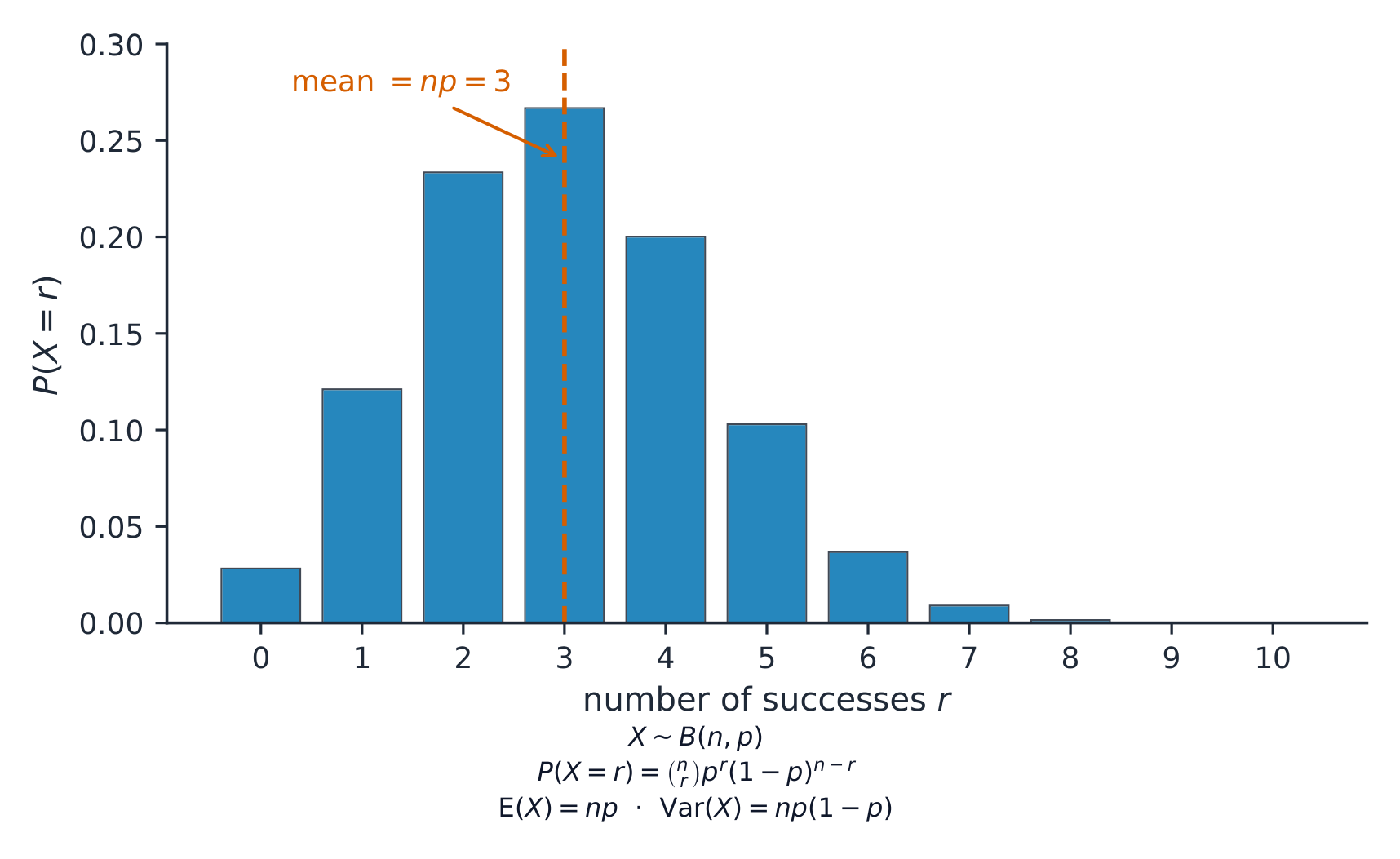
• the binomial distribution 二项分布 $X \sim B(n, p)$, for the number of successes in $n$ independent trials: $P(X = r) = \binom{n}{r}p^r(1-p)^{n-r}$, with $E(X) = np$ and $\mathrm{Var}(X) = np(1-p)$;
• the geometric distribution 几何分布, for the trial on which the first success happens: $P(X = r) = (1-p)^{r-1}p$, with $E(X) = \dfrac{1}{p}$.

Worked example. $X \sim B(10, 0.3)$. Find $P(X = 2)$ and $E(X)$.

The distribution $B(10,0.3)$: each bar is $P(X=r)$, clustered around the mean $np=3$.

A Galton board: balls falling through pins pile up into the bell-shaped normal distribution.

The normal distribution 正态分布 models a continuous random variable 连续型随机变量 with a symmetric bell shape. Write $X \sim N(\mu, \sigma^2)$, where $\mu$ is the mean and $\sigma$ is the standard deviation. To use the tables, by standardisation 标准化 convert to the variable $Z \sim N(0, 1)$:

A Galton board: balls fall through rows of pegs and pile up into the bell-shaped normal distribution Then $P(X < x) = P\!\left(Z < \dfrac{x - \mu}{\sigma}\right)$, which you read from the normal table $\Phi$.

A normal probability is an area under the bell curve; standardizing rescales it to $Z\sim N(0,1)$.

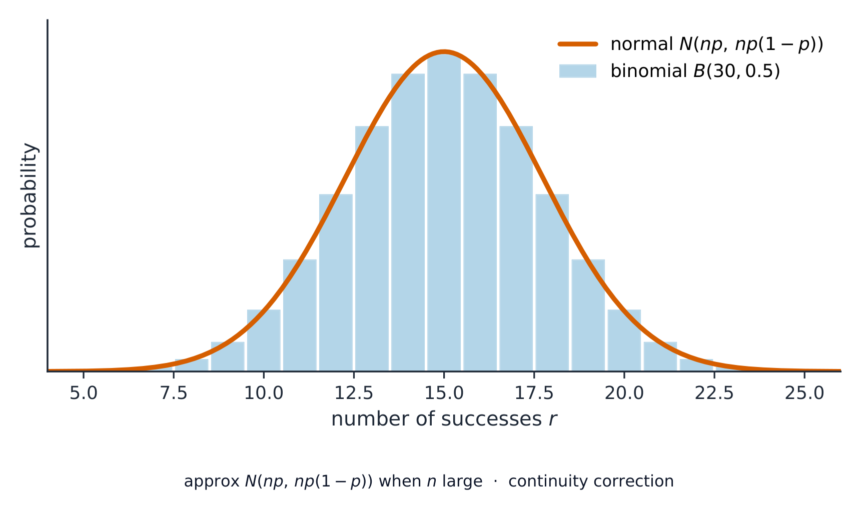
The normal distribution is also a good approximation 近似 to the binomial when $n$ is large. Because you replace a discrete variable by a continuous one, apply a continuity correction 连续性校正 (adjust by $0.5$).

When $n$ is large the binomial bars follow a normal curve of the same mean and variance.

Worked example. Bags of rice have mass $X \sim N(\mu, 0.14^2)$. Given that $P(X < 1.48) = 0.22$, find $\mu$.

From the table, $P(Z < z) = 0.22$ gives $z = -0.772$. So

• Decide whether order matters: permutations ($^nP_r$) when it does, combinations ($^nC_r$) when it does not.
• For a discrete random variable, check the probabilities sum to $1$ and use $E(X) = \sum x\,P(X=x)$.
• For the normal distribution, standardise with $z = (x - \mu)/\sigma$, sketch and shade, then read the table.
• Apply a continuity correction when approximating a discrete variable by the normal.