This handout covers Topic 6: Probability & Statistics 概率统计 2. It adds the Poisson model, combining random variables, continuous distributions, and the ideas of estimation and testing.
Probability & Statistics 2
A-Level Mathematics · Topic 6
 10:06
10:06
Probability & Statistics 2
Cambridge, the nineteen-twenties. At a garden party, a lady says something surprising. She can taste, she claims, whether the milk was poured into the cup…
English narration · English + 中文 subtitles burned in
6.1
The Poisson distribution

Syllabus
| Candidates should be able to: | Notes and examples |
|---|---|
| • use formulae to calculate probabilities for the distribution $\text{Po}(\lambda)$ | |
| • use the fact that if $X \sim \text{Po}(\lambda)$ then the mean and variance of $X$ are each equal to $\lambda$ | Proofs are not required. |
| • understand the relevance of the Poisson distribution to the distribution of random events, and use the Poisson distribution as a model | |
| • use the Poisson distribution as an approximation to the binomial distribution where appropriate | The conditions that $n$ is large and $p$ is small should be known; $n > 50$ and $np < 5$, approximately. |
| • use the normal distribution, with continuity correction, as an approximation to the Poisson distribution where appropriate. | The condition that $\lambda$ is large should be known; $\lambda > 15$, approximately. |
Source: Cambridge International syllabus
The Poisson distribution 泊松分布 $X \sim \mathrm{Po}(\lambda)$ models the number of random events in a fixed interval, when events happen at a steady average rate $\lambda$:
$$P(X = r) = e^{-\lambda}\frac{\lambda^r}{r!}.$$
For a Poisson variable the mean and the variance are both equal to $\lambda$. The Poisson distribution is a good approximation 近似 to the binomial distribution when $n$ is large and $p$ is small. The normal distribution (with continuity correction) approximates the Poisson when $\lambda$ is large.
Worked example. $X \sim \mathrm{Po}(3)$. Find $P(X = 2)$.
$$P(X = 2) = e^{-3}\frac{3^2}{2!} = e^{-3}\times 4.5 = 0.224.$$

Explore
The Poisson distribution
Change the mean λ. Poisson models the number of random events in a fixed interval — rare events give a skewed shape.
Vocabulary
Train
| English |
|---|
| Poisson distribution/ˈpɔɪsn ˌdɪstrɪˈbjuːʃn/ |
| approximation/əˌprɒksɪˈmeɪʃn/ |
6.2
Linear combinations of random variables
Syllabus
| Candidates should be able to: | Notes and examples |
|---|---|
| • use, when solving problems, the results that – $\text{E}(aX + b) = a\text{E}(X) + b$ and $\text{Var}(aX + b) = a^2\text{Var}(X)$ – $\text{E}(aX + bY) = a\text{E}(X) + b\text{E}(Y)$ – $\text{Var}(aX + bY) = a^2\text{Var}(X) + b^2\text{Var}(Y)$ for independent $X$ and $Y$ – if $X$ has a normal distribution then so does $aX + b$ – if $X$ and $Y$ have independent normal distributions then $aX + bY$ has a normal distribution – if $X$ and $Y$ have independent Poisson distributions then $X + Y$ has a Poisson distribution. | Proofs of these results are not required. |
Source: Cambridge International syllabus
When you change a variable by a linear rule, the expectation 期望 (mean) and variance 方差 follow these rules:
$$E(aX + b) = aE(X) + b, \qquad \mathrm{Var}(aX + b) = a^2\,\mathrm{Var}(X).$$
For two independent variables $X$ and $Y$:
$$E(aX + bY) = aE(X) + bE(Y), \qquad \mathrm{Var}(aX + bY) = a^2\,\mathrm{Var}(X) + b^2\,\mathrm{Var}(Y).$$
Two useful facts: if $X$ has a normal distribution 正态分布 then so does $aX + b$; and the sum of independent Poisson variables is again Poisson.
Worked example. $X$ has mean $5$ and variance $4$. Find $E(3X - 1)$ and $\mathrm{Var}(3X - 1)$.
$$E(3X - 1) = 3(5) - 1 = 14, \qquad \mathrm{Var}(3X - 1) = 3^2 \times 4 = 36.$$
Explore
Linear combination lab
E(aX + b) = aE(X) + b
Change a scaling factor and see how the expected value scales.
Vocabulary
Train
| English |
|---|
| expectation/ekspɪkˈteɪʃn/ |
| variance/ˈveərɪəns/ |
| normal distribution/ˈnɔːml ˌdɪstrɪˈbjuːʃn/ |
6.3
Continuous random variables
Syllabus
| Candidates should be able to: | Notes and examples |
|---|---|
| • understand the concept of a continuous random variable, and recall and use properties of a probability density function | For density functions defined over a single interval only; the domain may be infinite, e.g. $\frac{3}{x^4}$ for $x \geqslant 1$. |
| • use a probability density function to solve problems involving probabilities, and to calculate the mean and variance of a distribution. | Including location of the median or other percentiles of a distribution by direct consideration of an area using the density function. Explicit knowledge of the cumulative distribution function is not included. |
Source: Cambridge International syllabus
A continuous random variable 连续型随机变量 can take any value in a range. Its probabilities come from a probability density function 概率密度函数 $f(x)$, with two key properties:
$$f(x) \geqslant 0, \qquad \int_{-\infty}^{\infty} f(x)\,dx = 1.$$
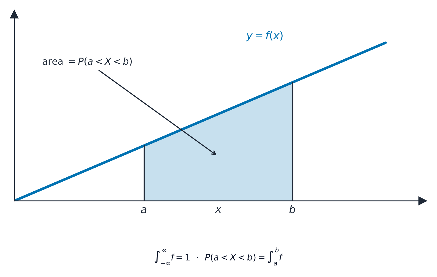
A probability is the area under $f$, and the mean is found by integration:
$$P(a < X < b) = \int_a^b f(x)\,dx, \qquad E(X) = \int_{-\infty}^{\infty} x\,f(x)\,dx.$$
The cumulative distribution function 累积分布函数 is $F(x) = P(X \leqslant x) = \int_{-\infty}^{x} f(t)\,dt$; the median 中位数 solves $F(m) = 0.5$, and other percentiles 百分位数 solve $F(x) = p$.
Worked example. A continuous variable has $f(x) = \tfrac12 x$ for $0 \leqslant x \leqslant 2$ (and $0$ elsewhere). Find $E(X)$.
$$E(X) = \int_0^2 x\cdot\tfrac12 x\,dx = \int_0^2 \tfrac12 x^2\,dx = \left[\tfrac{x^3}{6}\right]_0^2 = \frac{8}{6} = \frac{4}{3}.$$
The variance uses the same idea, $\mathrm{Var}(X)=\displaystyle\int_{-\infty}^{\infty}x^2 f(x)\,dx-\big(E(X)\big)^2$. For the same $f(x)=\tfrac12 x$ on $[0,2]$: $\displaystyle\int_0^2 x^2\cdot\tfrac12 x\,dx=\left[\tfrac{x^4}{8}\right]_0^2=2$, so $\mathrm{Var}(X)=2-\left(\tfrac43\right)^2=2-\tfrac{16}{9}=\tfrac{2}{9}$.
Explore
Area = probability
P(a < X < b) = ∫ f(x) dx
For a continuous variable, probability is the area under the density curve between two values.
Vocabulary
Train
| English |
|---|
| continuous random variable/kənˈtɪnjuːəs ˈrændəm ˈveərɪəbl/ |
| probability density function/ˌprɒbəˈbɪlɪti ˈdensɪti ˈfʌŋkʃn/ |
| cumulative distribution function/ˈkjuːmjʊlətɪv ˌdɪstrɪˈbjuːʃn ˈfʌŋkʃn/ |
| median/ˈmiːdiːən/ |
| percentiles/pəˈsentaɪlz/ |
6.4
Sampling and estimation

Syllabus
| Candidates should be able to: | Notes and examples |
|---|---|
| • understand the distinction between a sample and a population, and appreciate the necessity for randomness in choosing samples | |
| • explain in simple terms why a given sampling method may be unsatisfactory | Including an elementary understanding of the use of random numbers in producing random samples. Knowledge of particular sampling methods, such as quota or stratified sampling, is not required. |
| • recognise that a sample mean can be regarded as a random variable, and use the facts that $\text{E}(\overline{X}) = \mu$ and that $\text{Var}(\overline{X}) = \frac{\sigma^2}{n}$ | |
| • use the fact that $\overline{X}$ has a normal distribution if $X$ has a normal distribution | |
| • use the Central Limit Theorem where appropriate | Only an informal understanding of the Central Limit Theorem (CLT) is required; for large sample sizes, the distribution of a sample mean is approximately normal. |
| • calculate unbiased estimates of the population mean and variance from a sample, using either raw or summarised data | Only a simple understanding of the term 'unbiased' is required, e.g. that although individual estimates will vary the process gives an accurate result 'on average'. |
| • determine and interpret a confidence interval for a population mean in cases where the population is normally distributed with known variance or where a large sample is used | |
| • determine, from a large sample, an approximate confidence interval for a population proportion. |
Source: Cambridge International syllabus
A sample 样本 is a small group chosen from the whole population 总体. A random sample needs randomness 随机性, so that every member has a fair chance of being chosen.
Some methods are unsatisfactory because they are biased 有偏: sampling only volunteers, or the first 20 people to arrive, over-represents certain kinds of people. A genuinely random sample uses random numbers – number every member of the population, then draw numbers (from a table or a generator) to decide who is in the sample.
The sample mean $\bar{X}$ is itself a random variable, with
$$E(\bar{X}) = \mu, \qquad \mathrm{Var}(\bar{X}) = \frac{\sigma^2}{n}.$$
By the Central Limit Theorem 中心极限定理, for a large sample $\bar{X}$ is approximately normal, whatever the shape of the population.

From a sample you can find unbiased estimates 无偏估计 of the population mean and variance. A confidence interval 置信区间 gives a range that probably contains the true mean. When the population is normal with known $\sigma$ (or the sample is large), a $95\%$ interval is
$$\bar{x} \pm 1.96\,\frac{\sigma}{\sqrt{n}}.$$

You can also find a confidence interval for a population proportion 总体比例 from a large sample.
Worked example. A sample of $n = 64$ has mean $\bar{x} = 50$, from a population with $\sigma = 8$. Find a $95\%$ confidence interval for the population mean.
$$50 \pm 1.96\times\frac{8}{\sqrt{64}} = 50 \pm 1.96 \;\Rightarrow\; (48.0,\ 52.0).$$
Explore
The sampling distribution
X̄ ~ N(μ, σ²/n)
By the Central Limit Theorem, sample means follow a normal curve — narrower for bigger samples.
Vocabulary
Train
| English |
|---|
| sample/ˈsæmpl/ |
| population/ˌpɒpjʊˈleɪʃn/ |
| randomness/ˈrændəmnəs/ |
| biased/ˈbaɪəst/ |
| Central Limit Theorem/ˈsentrəl ˈlɪmɪt ˈθɪərəm/ |
| unbiased estimates/ʌnˈbaɪəst ˈestɪməts/ |
| confidence interval/ˈkɒnfɪdəns ˈɪntəvl/ |
| population proportion/ˌpɒpjʊˈleɪʃn prəˈpɔːʃn/ |
6.5
Hypothesis tests

Syllabus
| Candidates should be able to: | Notes and examples |
|---|---|
| • understand the nature of a hypothesis test, the difference between one-tailed and two-tailed tests, and the terms null hypothesis, alternative hypothesis, significance level, rejection region (or critical region), acceptance region and test statistic | Outcomes of hypothesis tests are expected to be interpreted in terms of the contexts in which questions are set. |
| • formulate hypotheses and carry out a hypothesis test in the context of a single observation from a population which has a binomial or Poisson distribution, using – direct evaluation of probabilities – a normal approximation to the binomial or the Poisson distribution, where appropriate | |
| • formulate hypotheses and carry out a hypothesis test concerning the population mean in cases where the population is normally distributed with known variance or where a large sample is used | |
| • understand the terms Type I error and Type II error in relation to hypothesis tests | |
| • calculate the probabilities of making Type I and Type II errors in specific situations involving tests based on a normal distribution or direct evaluation of binomial or Poisson probabilities. |
Source: Cambridge International syllabus
A hypothesis test 假设检验 uses sample data to judge a claim. You set up two statements: the null hypothesis 原假设 $H_0$ (the claim being tested, usually "no change") and the alternative hypothesis 备择假设 $H_1$ (what you suspect instead). The test is one-tailed 单尾 if $H_1$ points one way (e.g. $\mu > 50$) and two-tailed 双尾 if it allows both ways ($\mu \neq 50$).
You fix a significance level 显著性水平 (often $5\%$), work out a test statistic 检验统计量 from the data, and see whether it lands in the rejection region 拒绝域 (also called the critical region); if it does you reject $H_0$, otherwise the statistic is in the acceptance region.
Two mistakes are possible: a Type I error 第一类错误 is rejecting $H_0$ when it is actually true; a Type II error 第二类错误 is accepting $H_0$ when it is actually false. You can find their probabilities from the rejection region: $P(\text{Type I})=P(\text{statistic in the rejection region}\mid H_0)$ – this equals the significance level – and $P(\text{Type II})=P(\text{statistic in the acceptance region}\mid H_1$ true for a stated value$)$, computed from the binomial, Poisson, or normal distribution.
Worked example. A population is claimed to have mean $50$, with $\sigma = 8$. A sample of $n = 64$ gives $\bar{x} = 52$. Test at the $5\%$ level whether the mean has changed.
$H_0\!: \mu = 50$ and $H_1\!: \mu \neq 50$ (two-tailed). The test statistic is
$$z = \frac{\bar{x} - \mu}{\sigma/\sqrt{n}} = \frac{52 - 50}{8/8} = 2.$$
The critical value at $5\%$ (two-tailed) is $1.96$. Since $2 > 1.96$, you reject $H_0$: there is evidence the mean has changed.
Worked example (a binomial test). A coin is claimed fair but suspected of landing heads too rarely: $H_0\!:p=0.5$, $H_1\!:p<0.5$. In $n=30$ tosses you see $X=9$ heads. Under $H_0$, $X\sim B(30,0.5)$, so the one-tailed tail probability is
$$P(X\leqslant 9)=\sum_{k=0}^{9}\binom{30}{k}(0.5)^{30}\approx 0.021.$$
Since $0.021<0.05$, reject $H_0$: the coin does seem biased against heads. (For large $n$ the binomial is approximated by a normal; a Poisson test works the same way for rare events. And here, if the rule is "reject when $X\leqslant 9$", then $P(\text{Type I})=P(X\leqslant 9\mid p=0.5)\approx0.021$.)
Explore
The rejection region
reject H₀ if z < −z*
The shaded tail is the rejection region — if the test statistic lands there, reject H₀.
Vocabulary
Train
| English |
|---|
| hypothesis test/haɪˈpɒθəsɪs test/ |
| null hypothesis/nʌl haɪˈpɒθəsɪs/ |
| alternative hypothesis/ɔːlˈtɜːnətɪv haɪˈpɒθəsɪs/ |
| one-tailed/wʌn teɪld/ |
| two-tailed/tuː teɪld/ |
| significance level/sɪɡˈnɪfɪkəns ˈlevl/ |
| test statistic/test stəˈtɪstɪk/ |
| rejection region/rɪˈdʒekʃn ˈriːdʒn/ |
| Type I error/taɪp aɪ ˈerə/ |
| Type II error/taɪp ˈtuː ˈerə/ |
| Probability & Statistics/ˌprɒbəˈbɪlɪti ænd stəˈtɪstɪks/ |
6.5
Exam tips
- Use the Poisson distribution for rare, random, independent events; its mean equals its variance ($= \lambda$).
- When combining independent random variables, variances add (they never subtract).
- For a hypothesis test, state $H_0$ and $H_1$, the significance level, the test statistic, and a conclusion in context.
- For a confidence interval, use the correct $z$ (or $t$) value and interpret it in words.
Interactive lessons on this topic
Work through it step by step, with instant-check exercises.