Skip to content · ⁨コンテンツへスキップ⁩

Differential Equations

AP Calculus BC · Topic 7 · ⁨トピック 7⁩

View Slides · ⁨查看幻灯片⁩ Train · ⁨練習する⁩
Video lesson for this topic · ⁨このトピックのビデオレッスン⁩ Open the video page · ⁨動画ページを開く⁩
8:26

微分方程式を用いたモデル化

通常は関数を与えられ、その傾きを求められます。微分方程式はその逆です。すべての点における傾きのルールを与えられて、…

English narration · English + 中文 subtitles burned in · ⁨英語ナレーション・英語+中文字幕 burning-in⁩

7.1

Modeling Situations with Differential Equations · ⁨微分方程式によるモデル化⁩

Syllabus · ⁨シラバス⁩
English

Enduring Understanding (FUN-7): Solving differential equations allows us to determine functions and develop models.

Learning Objective FUN-7.A: Interpret verbal statements of problems as differential equations involving a derivative expression.

  • FUN-7.A.1 Differential equations relate a function of an independent variable and the function's derivatives.
日本語

持続的理解 (FUN-7): 微分方程式を解くことで、関数を決定し、モデルを作成できる。

学習目標 FUN-7.A: 問題の言語的な記述を、導関数式を含む微分方程式として解釈する。

  • FUN-7.A.1 微分方程式は、独立変数の関数とその導関数の関係を表す。
Source: College Board AP Course and Exam Description · ⁨出典: College Board AP コースおよび試験説明書⁩

English

A differential equation 微分方程 relates a function to its derivatives. Many real situations are described by a rate: "the population grows at a rate proportional to its size" becomes $\dfrac{dP}{dt}=kP$. Setting up the equation from a verbal description – identifying what changes and what it is proportional to – is the first skill.

日本語

微分方程式は関数とその導関数との関係を表します。多くの現実の事象は変化率で記述されます。「個体数がその大きさに比例して増加する」ことは $\dfrac{dP}{dt}=kP$ となります。言葉での説明から方程式を立てる(何が変化しているか、それに比例的是什么かを特定する)ことが最初のスキルです。

7.2

Verifying Solutions for Differential Equations · ⁨微分方程式の解の確認⁩

Syllabus · ⁨シラバス⁩
English

Enduring Understanding (FUN-7): Solving differential equations allows us to determine functions and develop models.

Learning Objective FUN-7.B: Verify solutions to differential equations.

  • FUN-7.B.1 Derivatives can be used to verify that a function is a solution to a given differential equation.
  • FUN-7.B.2 There may be infinitely many general solutions to a differential equation.
日本語

持続的理解 (FUN-7): 微分方程式を解くことで、関数を決定し、モデルを作成できる。

学習目標 FUN-7.B: 微分方程式の解を検証する。

  • FUN-7.B.1 導関数を用いて、ある関数が与えられた微分方程式の解であることを確認できる。
  • FUN-7.B.2 微分方程式には、無数の一般解が存在することがある。

Source: College Board AP Course and Exam Description · ⁨出典: College Board AP コースおよび試験説明書⁩

English

A solution is a function that satisfies the equation. To verify a proposed solution, differentiate it and substitute into the equation, checking that both sides agree. A general solution contains a constant $C$; a particular solution fixes $C$ from a condition.

日本語

解とは、方程式を満たす関数のことです。検証するには、提案された解を微分して方程式に代入し、両辺が一致するか確認します。一般解には定数 $C$ が含まれ、特殊解は条件から $C$ を固定したものです。

7.3

Sketching Slope Fields · ⁨傾き場の描画⁩

Syllabus · ⁨シラバス⁩
Enduring UnderstandingLearning ObjectiveEssential Knowledge

FUN-7
Solving differential equations allows us to determine functions and develop models.

FUN-7.C
Estimate solutions to differential equations.

  • FUN-7.C.1 A slope field is a graphical representation of a differential equation on a finite set of points in the plane.
  • FUN-7.C.2 Slope fields provide information about the behavior of solutions to first-order differential equations.

Source: College Board AP Course and Exam Description · ⁨出典: College Board AP コースおよび試験説明書⁩

English
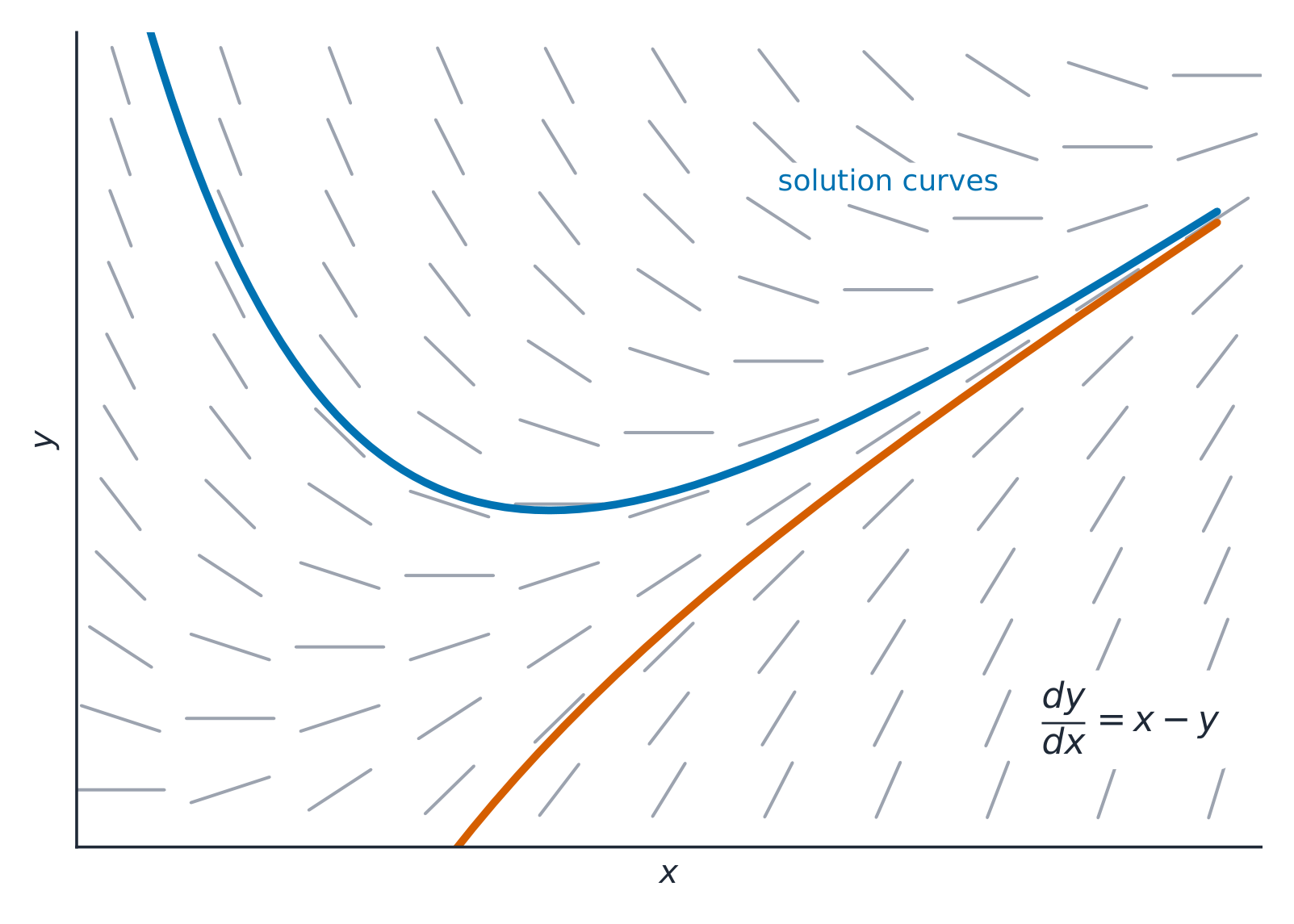
Slope fields & solution curves

A slope field 斜率场 draws a short line segment at many points, each with the slope $\dfrac{dy}{dx}$ the equation gives there. It pictures the family of solution curves without solving. To sketch one, evaluate the right-hand side at each grid point and draw a segment of that slope.

日本語
傾き場と解曲線

傾き場は、方程式が示す傾き $\dfrac{dy}{dx}$ を持つ短い線分を多数の点に描きます。解を解くことなく、解曲線の家族を可視化します。スケッチするには、各格子点で右辺を計算し、その傾きの線分を描きます。

傾き場はすべての地点で勾配を示し、解曲線はその方向に従います
Explore · ⁨探索⁩

Read a differential equation as a slope field · ⁨微分方程式を傾き場として読む⁩

A slope field draws the slope $dy/dx$ at each point. A solution curve threads through, always tangent to the little segments — you can sketch it by following the flow. · ⁨傾き場 は各点における傾き $dy/dx$ を描きます。解曲線は小さな線分常に接しながら通っていき、流れに沿ってスケッチすることができます。⁩

Vocabulary · ⁨語彙⁩ Train · ⁨練習する⁩
English 日本語
differential equation/ˌdɪfəˈrenʃl ɪˈkweɪʒn/ 微分方程式
slope field/sləʊp fiːld/ 傾き場
7.4

Reasoning Using Slope Fields · ⁨傾き場を用いた推論⁩

Syllabus · ⁨シラバス⁩
English

Enduring Understanding (FUN-7): Solving differential equations allows us to determine functions and develop models.

Learning Objective FUN-7.C: Estimate solutions to differential equations.

  • FUN-7.C.3 Solutions to differential equations are functions or families of functions.
日本語

持続的理解 (FUN-7): 微分方程式を解くことで、関数を決定し、モデルを作成できる。

学習目標 FUN-7.C: 微分方程式の解を推定する。

  • FUN-7.C.3 微分方程式の解は、関数または関数の族である。

Source: College Board AP Course and Exam Description · ⁨出典: College Board AP コースおよび試験説明書⁩

English

A solution curve follows the segments like a boat following a current. From a slope field you can sketch the particular solution through a given point, describe long-run behavior, and locate where solutions level off (slopes near zero) – reasoning about solutions purely from the picture.

日本語

解曲線は川の流れに従う船のように、線分に沿って進みます。傾き場から特定の点を通る特殊解をスケッチしたり、長期行動を記述したり、解が平坦になる場所(傾きがゼロに近い場所)を特定したりできます – 図のみから解について推論する能力です。

7.5

Approximating Solutions Using Euler's Method · ⁨Euler法を用いた近似解⁩

Syllabus · ⁨シラバス⁩
English

Enduring Understanding (FUN-7): Solving differential equations allows us to determine functions and develop models.

Learning Objective FUN-7.C: Estimate solutions to differential equations.

  • FUN-7.C.4 Euler's method provides a procedure for approximating a solution to a differential equation or a point on a solution curve. BC ONLY
日本語

持続的理解 (FUN-7): 微分方程式を解くことで、関数を決定し、モデルを作成できる。

学習目標 FUN-7.C: 微分方程式の解を推定する。

  • FUN-7.C.4 オイラー法は、微分方程式の解を近似したり、解曲線上の点を求めたりするための手順を提供する。BC ONLY

Source: College Board AP Course and Exam Description · ⁨出典: College Board AP コースおよび試験説明書⁩

English
Euler's method

Euler's method 欧拉方法 approximates a solution numerically by stepping along the slope field. Starting from a known point, take a small step $\Delta x$ and update:

$$y_{\text{new}}=y_{\text{old}}+\frac{dy}{dx}\cdot\Delta x.$$
Repeat for each step. Smaller steps give a better approximation. (This is a BC-only technique.)

Exam skill: be able to carry out two or three Euler steps by hand from a table, and know that Euler's method under- or over-estimates depending on the solution's concavity.

Worked example. Approximate $y(1)$ for $\dfrac{dy}{dx}=x+y$, $y(0)=1$, with step $\Delta x=0.5$. Step 1: slope at $(0,1)$ is $0+1=1$, so $y(0.5)\approx 1+1(0.5)=1.5$. Step 2: slope at $(0.5,1.5)$ is $0.5+1.5=2$, so $y(1)\approx 1.5+2(0.5)=2.5$.

日本語
Euler's method

Euler法は、傾き場に沿ってステップを踏むことで数値的に解を近似します。既知の点から始め、小さなステップ $\Delta x$ を取り、更新します:

$$y_{\text{new}}=y_{\text{old}}+\frac{dy}{dx}\cdot\Delta x.$$
各ステップで繰り返します。ステップが小さいほど近似は良くなります。(これはBC-onlyの技法です。)

Exam skill: テーブルから手動でEulerステップを2〜3回実行でき、Euler法が解のconcavityに応じてunder- or over-estimates(過小評価または過大評価)することを知っています。

Worked example. $y(1)$ を近似します。 $\dfrac{dy}{dx}=x+y$ 、 $y(0)=1$ で、ステップ $\Delta x=0.5$ を使用します。 Step 1: $(0,1)$ での傾きは $0+1=1$ なので、 $y(0.5)\approx 1+1(0.5)=1.5$ です。 Step 2: $(0.5,1.5)$ での傾きは $0.5+1.5=2$ なので、 $y(1)\approx 1.5+2(0.5)=2.5$ です。

Vocabulary · ⁨語彙⁩ Train · ⁨練習する⁩
English 日本語
Euler's method/ˈɔɪləz ˈmeθəd/ オイラー法
separable/ˈsepərəbl/ 変数分離可能
initial condition/ɪˈnɪʃl kənˈdɪʃn/ 初期条件
exponential growth or decay/ˌekspəˈnenʃl ɡrəʊθ ɔː dɪˈkeɪ/ 指数関数的増加または減少
logistic model/ləˈdʒɪstɪk ˈmɒdl/ ロジスティックモデル
7.6

Finding General Solutions Using Separation of Variables · ⁨変数分離法による一般解の導出⁩

Syllabus · ⁨シラバス⁩
English

Enduring Understanding (FUN-7): Solving differential equations allows us to determine functions and develop models.

Learning Objective FUN-7.D: Determine general solutions to differential equations.

  • FUN-7.D.1 Some differential equations can be solved by separation of variables.
  • FUN-7.D.2 Antidifferentiation can be used to find general solutions to differential equations.
日本語

持続的理解 (FUN-7): 微分方程式を解くことで、関数を決定し、モデルを作成できる。

学習目標 FUN-7.D: 微分方程式の一般解を求める。

  • FUN-7.D.1 一部の微分方程式は、変数分離法によって解ける。
  • FUN-7.D.2 原始積分を用いて、微分方程式の一般解を求めることができる。

Source: College Board AP Course and Exam Description · ⁨出典: College Board AP コースおよび試験説明書⁩

English

A separable 可分离 differential equation can be written with all the $y$'s on one side and all the $x$'s on the other, then integrated:

$$\frac{dy}{dx}=g(x)h(y)\ \Rightarrow\ \int\frac{dy}{h(y)}=\int g(x)\,dx.$$
This produces the general solution (with a $+C$), the main analytic method for solving differential equations in this course.

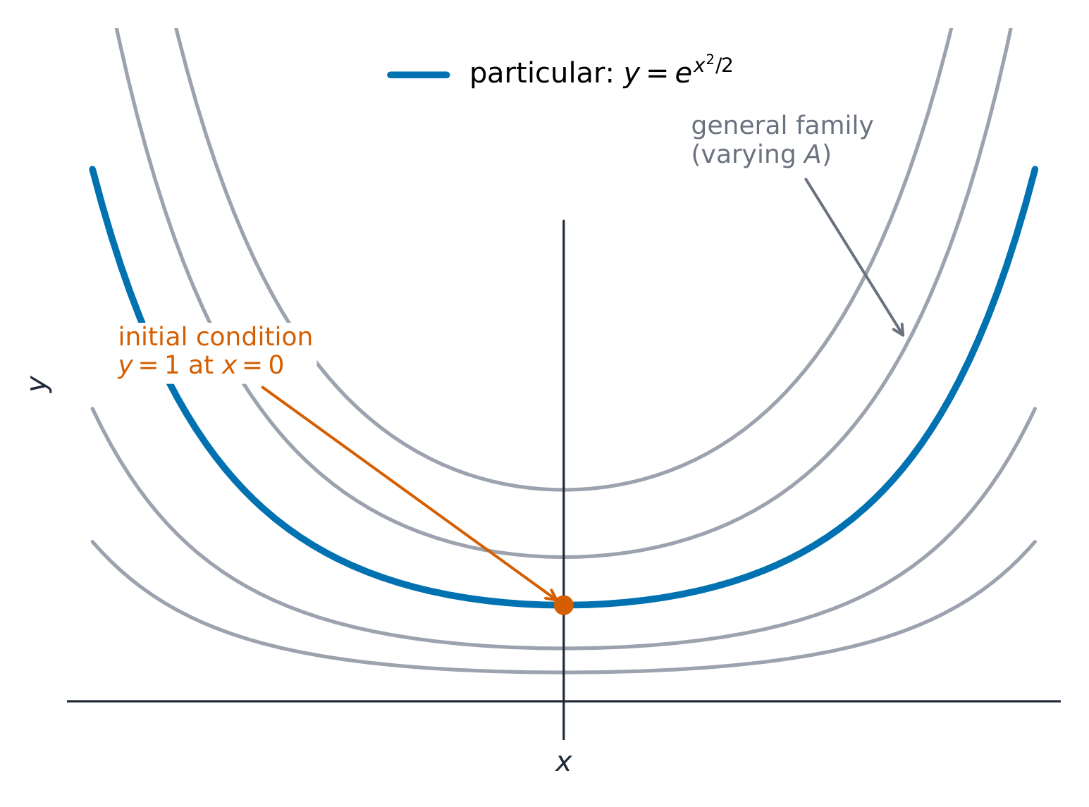
Worked example. Solve $\dfrac{dy}{dx}=xy$ with $y(0)=2$. Separating, $\int\frac{dy}{y}=\int x\,dx$ gives $\ln|y|=\frac{x^2}{2}+C$, so $y=Ae^{x^2/2}$. The condition $y(0)=2$ gives $A=2$, so $y=2e^{x^2/2}$.

日本語
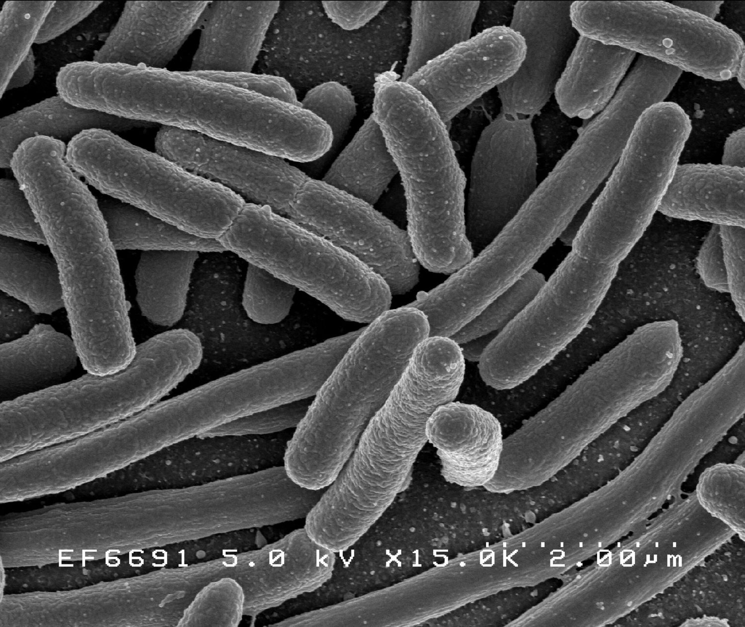
顕微鏡下の大腸菌:微分方程式は指数関数的増殖をモデル化します

可分微分方程式は、すべての $y$ を片側に、すべての $x$ を他方に置いてから積分できる形に書けます:

$$\frac{dy}{dx}=g(x)h(y)\ \Rightarrow\ \int\frac{dy}{h(y)}=\int g(x)\,dx.$$
これにより一般解(定数 $+C$ を含む)が得られ、これが本課程における微分方程式を解く主要な解析的手法です。

Worked example. $\dfrac{dy}{dx}=xy$ を $y(0)=2$ で解きます。可分化すると、 $\int\frac{dy}{y}=\int x\,dx$ から $\ln|y|=\frac{x^2}{2}+C$ となり、したがって $y=Ae^{x^2/2}$ です。条件 $y(0)=2$ から $A=2$ が得られるため、 $y=2e^{x^2/2}$ となります。

7.7

Finding Particular Solutions Using Initial Conditions · ⁨初期条件を用いた特殊解の探索⁩

Syllabus · ⁨シラバス⁩
English

Enduring Understanding (FUN-7): Solving differential equations allows us to determine functions and develop models.

Learning Objective FUN-7.E: Determine particular solutions to differential equations.

  • FUN-7.E.1 A general solution may describe infinitely many solutions to a differential equation. There is only one particular solution passing through a given point.
  • FUN-7.E.2 The function $F$ defined by $F(x) = y_0 + \int_a^x f(t)\,dt$ is a particular solution to the differential equation $\dfrac{dy}{dx} = f(x)$, satisfying $F(a) = y_0$.
  • FUN-7.E.3 Solutions to differential equations may be subject to domain restrictions.
日本語

持続的理解 (FUN-7): 微分方程式を解くことで、関数を決定し、モデルを作成できる。

学習目標 FUN-7.E: 微分方程式の特解を求める。

  • FUN-7.E.1 一般解は、微分方程式の無数の解を表すことがある。ある点を通る特解は一つだけである。
  • FUN-7.E.2 関数 $F$ は、関数 $F(x) = y_0 + \int_a^x f(t)\,dt$ によって定義され、微分方程式 $\dfrac{dy}{dx} = f(x)$ の particular solution であり、$F(a) = y_0$ を満たす。
  • FUN-7.E.3 微分方程式の解には、定義域の制限が課されることがある。

Source: College Board AP Course and Exam Description · ⁨出典: College Board AP コースおよび試験説明書⁩

English

An initial condition 初始条件 (a known point, e.g. $y(0)=5$) pins down the constant $C$. Solve for the general solution, substitute the condition to find $C$, then write the particular solution. Watch the domain – a particular solution is valid only on the interval containing the initial point.

日本語

初期条件(既知の点、例: $y(0)=5$ )は定数 $C$ を決定します。一般解を解き、条件を代入して $C$ を見つけ、特殊解を書きます。定義域に注意してください – 特殊解は初期点を含む区間でのみ有効です。

定数により曲線の族が得られ、初期条件によって1つの曲線が選ばれる
7.8

Exponential Models with Differential Equations · ⁨微分方程式による指数関数モデル⁩

Syllabus · ⁨シラバス⁩
Enduring UnderstandingLearning ObjectiveEssential Knowledge

FUN-7
Solving differential equations allows us to determine functions and develop models.

FUN-7.F
Interpret the meaning of a differential equation and its variables in context.

  • FUN-7.F.1 Specific applications of finding general and particular solutions to differential equations include motion along a line and exponential growth and decay.
  • FUN-7.F.2 The model for exponential growth and decay that arises from the statement "The rate of change of a quantity is proportional to the size of the quantity" is $\dfrac{dy}{dt} = ky$.

FUN-7.G
Determine general and particular solutions for problems involving differential equations in context.

  • FUN-7.G.1 The exponential growth and decay model, $\dfrac{dy}{dt} = ky$, with initial condition $y = y_0$ when $t = 0$, has solutions of the form $y = y_0 e^{kt}$.

Source: College Board AP Course and Exam Description · ⁨出典: College Board AP コースおよび試験説明書⁩

English
Exponential vs logistic growth

The equation $\dfrac{dy}{dt}=ky$ says the rate of change is proportional to the amount – giving exponential growth or decay 指数增长. Separating variables yields

$$y=y_0 e^{kt},$$
with $k>0$ for growth and $k<0$ for decay. This models unrestricted population growth, radioactive decay, and continuously compounded interest.

日本語
指数関数的成長とロジスティック成長

方程式 $\dfrac{dy}{dt}=ky$ は、変化率が量に proportional (比例)であることを示しており、指数関数的増減を与えます。変数分離を行うと

$$y=y_0 e^{kt},$$
が得られ、 $k>0$ は増減、 $k<0$ は減少を表します。これは無制限の個体数増減、放射性崩壊、複利の連続複利をモデル化します。

冷めていくコーヒー:ニュートンの冷却則は古典的な微分方程式モデルです
Explore · ⁨探索⁩

An exponential growth/decay model · ⁨指数関数的増減モデル⁩

y = a·e^(bx) + c

The equation $dy/dt=ky$ has exponential solutions: quantity changes at a rate proportional to itself, giving unbounded growth ($k>0$) or decay to zero ($k<0$). · ⁨方程式 $dy/dt=ky$ には 指数関数 的な解があります:量は自身に比例した速度で変化し、無制限の増加($k>0$)またはゼロへの減少($k<0$)をもたらします。⁩

7.9

Logistic Models with Differential Equations · ⁨微分方程式によるロジスティックモデル⁩

Syllabus · ⁨シラバス⁩
English

Enduring Understanding (FUN-7): Solving differential equations allows us to determine functions and develop models.

Learning Objective FUN-7.H: Interpret the meaning of the logistic growth model in context. BC ONLY

  • FUN-7.H.1 The model for logistic growth that arises from the statement "The rate of change of a quantity is jointly proportional to the size of the quantity and the difference between the quantity and the carrying capacity" is $\dfrac{dy}{dt} = ky(a - y)$. BC ONLY
  • FUN-7.H.2 The logistic differential equation and initial conditions can be interpreted without solving the differential equation. BC ONLY
  • FUN-7.H.3 The limiting value (carrying capacity) of a logistic differential equation as the independent variable approaches infinity can be determined using the logistic growth model and initial conditions. BC ONLY
  • FUN-7.H.4 The value of the dependent variable in a logistic differential equation at the point when it is changing fastest can be determined using the logistic growth model and initial conditions. BC ONLY
日本語

持続的理解 (FUN-7): 微分方程式を解くことで、関数を決定し、モデルを作成できる。

学習目標 FUN-7.H: コンテキストにおけるロジスティック成長モデルの意味を解釈する。BC ONLY

  • FUN-7.H.1 「ある量の変化率が、その量の大きさとその量と carrying capacity の差との積に比例する」という記述から導かれるロジスティック成長のモデルは $\dfrac{dy}{dt} = ky(a - y)$ である。BC ONLY
  • FUN-7.H.2 ロジスティック微分方程式と初期条件は、微分方程式を解くことなく解釈できる。BC ONLY
  • FUN-7.H.3 独立変数が無限大に近づくときのロジスティック微分方程式の極限値(carrying capacity)は、ロジスティック成長モデルと初期条件を用いて決定できる。BC ONLY
  • FUN-7.H.4 ロジスティック微分方程式において依存変数の値が最も速く変化している時点での値は、ロジスティック成長モデルと初期条件を用いて決定できる。BC ONLY

Source: College Board AP Course and Exam Description · ⁨出典: College Board AP コースおよび試験説明書⁩

English

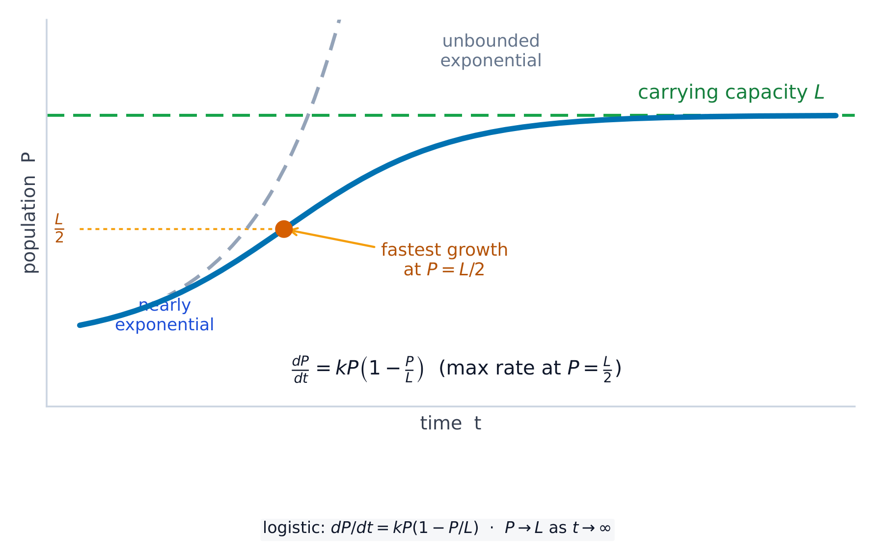
Real growth is limited by resources, so the logistic model 逻辑斯蒂模型 adds a carrying capacity 环境容纳量 $L$:

$$\frac{dP}{dt}=kP\!\left(1-\frac{P}{L}\right).$$
Growth is nearly exponential when $P$ is small, slows as $P$ approaches $L$, and stops at $P=L$. Key BC facts: the population levels off at $L$ ($\lim_{t\to\infty}P=L$), and it grows fastest when $P=\tfrac{L}{2}$ (the inflection point of the S-shaped curve). You are expected to read $L$ and the fastest-growth value directly from the equation.

Worked example. For $\dfrac{dP}{dt}=0.05\,P\!\left(1-\dfrac{P}{2000}\right)$, the carrying capacity is $L=2000$ (the population levels off there), and growth is fastest when $P=\dfrac{L}{2}=1000$ – both read straight off the equation, no solving needed.

日本語

実際の成長は資源によって制限されるため、ロジスティックモデルは carrying capacity $L$ を追加します:

$$\frac{dP}{dt}=kP\!\left(1-\frac{P}{L}\right).$$
$P$ が小さいとき、増殖はほぼ指数関数的であり、$P$ が $L$ に近づくにつれて減速し、$P=L$ で停止します。AP BCの重要な事実: 個体数は $L$ で一定になる ($\lim_{t\to\infty}P=L$)、また $P=\tfrac{L}{2}$ のときに最も速く増殖する (S字曲線の変曲点)。$L$ と最大増殖値を方程式から直接読み取ることを期待されます。

** worked example.** $\dfrac{dP}{dt}=0.05\,P\!\left(1-\dfrac{P}{2000}\right)$ について、環境収容力は $L=2000$ (個体数がそこで一定になる) であり、増殖が最も速いのは $P=\dfrac{L}{2}=1000$ です – これらは方程式からそのまま読み取れます。計算は不要です。

logisticモデルはP=L/2で最も速く増殖し、環境収容力Lで一定になります
Vocabulary · ⁨語彙⁩ Train · ⁨練習する⁩
English 日本語
carrying capacity/ˈkæriɪŋ kəˈpæsɪti/ 環境収容力
7.9

Exam tips · ⁨試験対策⁩

English
  • Solve a separable equation by getting all $y$ on one side and all $x$ on the other, then integrating both sides (add $+C$ once).
  • Use the initial condition to find $C$ (a particular solution).
  • Sketch or read a slope field: the little segments show $\tfrac{dy}{dx}$ at each point, and a solution curve follows them.
  • Recognise exponential models $\tfrac{dy}{dt}=ky\Rightarrow y=Ce^{kt}$ (growth/decay).
  • A differential equation gives the slope — you must integrate to recover the function.
日本語
  • 可分方程式 を解くには、$y$ を片方、$x$ を他方に集め、両辺を積分します(定数 $+C$ を加えます)。
  • 初期条件を用いて $C$ を見つけ(特殊解を得ます)。
  • 傾き場 を描画または読み取ります。各点における小さな線分は $\tfrac{dy}{dx}$ を示しており、解曲線はその方向に従います。
  • 指数関数モデル $\tfrac{dy}{dt}=ky\Rightarrow y=Ce^{kt}$(増減)を識別します。
  • 微分方程式は傾きを与えます。関数を復元するためには積分を行う必要があります。

Interactive lessons on this topic · ⁨このトピックのインタラクティブ授業⁩

Work through it step by step, with instant-check exercises. · ⁨一歩ずつ進め、即時チェック付きの問題で学習します。⁩

Past Papers · ⁨過去問⁩

More topics in AP Calculus BC · ⁨AP Calculus BC の他のトピック⁩

Log in or create account · ⁨ログインまたはアカウント作成⁩

IGCSE, A-Level & AP