Capacitance · ⁨קיבול⁩

A capacitor 电容器 stores charge. The simplest one is two parallel conductor 导体 plates with an insulator 绝缘体 (a dielectric 电介质, or just vacuum 真空 / air) between them. Connected to a battery, charge $+Q$ builds up on one plate and $-Q$ on the other, with a potential difference 电势差 $V$ across the gap.

How the plates become charged. Connect the plates to a battery and electrons flow, through the battery, from the plate joined to the positive terminal 接线端 to the plate joined to the negative terminal. One plate is left with charge $+Q$ and the other gains $-Q$: the charges are always equal and opposite, so the capacitor as a whole stays neutral. The flow stops when the p.d. between the plates equals the e.m.f. of the battery. Nothing crosses the gap; the insulator is what keeps the charge separated.

The capacitance 电容 $C$ of any capacitor (or any isolated conductor) is

This applies to:

• an isolated sphere holding charge $Q$ at potential $V$ (zero at infinity). For radius $r$, $V = Q/(4\pi\varepsilon_{0}r)$, so $C = 4\pi\varepsilon_{0} r$.
• a parallel-plate capacitor: charges $\pm Q$ on the plates, p.d. $V$ between them.

Unit: farad 法拉 (F) $= \text{C V}^{-1}$. A farad is huge, so real capacitors run from $\text{pF}$ to $\text{mF}$.

Capacitance is constant for a given capacitor (set by its size and dielectric). Doubling the charge doubles the voltage, so $C = Q/V$ stays the same.

The two-mark definitions. For a parallel-plate capacitor: the charge on one plate per unit potential difference between the plates. For an isolated sphere (or any isolated conductor): the charge on the conductor per unit potential. The examiner looks for "charge per unit p.d." (or "per unit potential") and, for the plates, that the charge is the charge on one plate and the p.d. is that between the plates. "The charge stored" is accepted; "the total charge on both plates" is not, because that total is zero.

What sets the capacitance. For parallel plates the capacitance is proportional to the plate area and inversely proportional to the separation $x$ ($C \propto 1/x$: halve the gap and the capacitance doubles), and it rises when a dielectric replaces the air. A question that states "$C$ is inversely proportional to $x$" and then moves the plates apart at constant charge is asking for $V = Q/C \propto x$: the p.d. rises in proportion. At constant p.d. (still connected to the supply) it is the charge that falls instead.

Worked example. A $100\ \mu\text{F}$ capacitor is charged to $12\ \text{V}$. Find the charge stored.

Worked example. An isolated metal sphere of radius $15\ \text{cm}$ is charged to a potential of $9.0 \times 10^{3}\ \text{V}$. Find its capacitance and its charge. It is then discharged to earth through a $120\ \text{M}\Omega$ resistor: find the time constant of the discharge.

The time constant is $RC = (1.2 \times 10^{8})(1.67 \times 10^{-11}) = 2.0 \times 10^{-3}\ \text{s}$: even through an enormous resistance the sphere loses its charge in milliseconds, because its capacitance is so small. Notice that $4\pi\varepsilon_{0} = 1/(8.99 \times 10^{9})$, so $C = r/(8.99 \times 10^{9})$ with $r$ in metres.

Combining capacitors

Capacitors in parallel share the same p.d. $V$. The total charge is the sum:

A parallel combination has larger capacitance than any one capacitor.

Capacitors in series carry the same charge $Q$. The total p.d. is the sum:

A series combination has smaller capacitance than any one capacitor.

Note: these rules are the opposite of those for resistors (resistors sum in series; capacitors sum in parallel), because $C = Q/V$ has $V$ on the bottom while $R = V/I$ has $I$ on the bottom.

Deriving the two rules

"Derive an expression for the combined capacitance" is a show that question, and the mark scheme wants the physics stated, not just the algebra.

• Series. The capacitors carry the same charge $Q$: the plate joined to the positive terminal loses electrons to the far plate of the next capacitor, so every plate in the chain holds $\pm Q$. The p.d.s add: $V = V_{1} + V_{2}$. With $V_{1} = Q/C_{1}$ and $V_{2} = Q/C_{2}$, and the combination defined by $V = Q/C$, dividing through by $Q$ gives $1/C = 1/C_{1} + 1/C_{2}$.
• Parallel. The capacitors have the same p.d. $V$, because each is connected directly across the supply. The charges add: $Q = Q_{1} + Q_{2} = C_{1}V + C_{2}V$, and $Q = CV$ for the combination, so $C = C_{1} + C_{2}$.

Two capacitors in series always give less than the smaller one; two equal capacitors $C$ give $C/2$ in series and $2C$ in parallel.

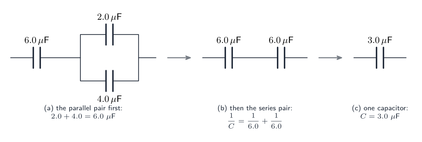
Worked example. A $6.0\ \mu\text{F}$ capacitor is in series with a parallel pair of $2.0\ \mu\text{F}$ and $4.0\ \mu\text{F}$. Find the total capacitance, and the charge on each capacitor when $12\ \text{V}$ is applied across the network.

Parallel pair: $2.0 + 4.0 = 6.0\ \mu\text{F}$. In series with $6.0\ \mu\text{F}$: $1/C = 1/6.0 + 1/6.0$, so $C = 3.0\ \mu\text{F}$. Total charge $Q = CV = (3.0 \times 10^{-6})(12) = 3.6 \times 10^{-5}\ \text{C}$: this is the charge on the $6.0\ \mu\text{F}$ capacitor (series, same charge), and it is shared by the parallel pair in the ratio of their capacitances (same p.d., $6.0\ \text{V}$ across each): the $2.0\ \mu\text{F}$ holds $1.2 \times 10^{-5}\ \text{C}$ and the $4.0\ \mu\text{F}$ holds $2.4 \times 10^{-5}\ \text{C}$. Check: they add to $3.6 \times 10^{-5}\ \text{C}$.

Worked example. Capacitors X and Y, each of capacitance $C$, are connected in series across a supply of voltage $V$; capacitors P and Q, each $C$, are connected in parallel across an identical supply. Compare the charge drawn from each supply and the energy stored in each arrangement.

Series: $C_{\text{s}} = C/2$, charge $Q_{\text{s}} = CV/2$, energy $\tfrac{1}{2} C_{\text{s}} V^{2} = CV^{2}/4$. Parallel: $C_{\text{p}} = 2C$, charge $2CV$, energy $CV^{2}$. The parallel arrangement draws four times the charge and stores four times the energy, because at the same supply voltage the energy is $\tfrac{1}{2} C V^{2}$ and the capacitance is four times larger. Asked which arrangement stores more energy from a given supply, the answer is always parallel.

Charging a capacitor from $0$ to $Q$ needs work, because each extra bit of charge is pushed against the p.d. already there. When the charge is $q$, the p.d. is $V(q) = q/C$, so adding a small charge $dq$ needs work $V\,dq$. The total work is

Using $V = Q/C$, this is the energy 能量 stored:

Worked example. Find the energy stored in a $100\ \mu\text{F}$ capacitor charged to $12\ \text{V}$.

Worked example. The graph of charge $Q$ against p.d. $V$ for a capacitor is a straight line through the origin passing through $(10\ \text{V},\ 1.2 \times 10^{-3}\ \text{C})$. Find the capacitance and the energy stored at $10\ \text{V}$, and then the extra energy stored when the p.d. is raised to $12\ \text{V}$.

The gradient of $Q$ against $V$ is $C = 1.2 \times 10^{-3}/10 = 1.2 \times 10^{-4}\ \text{F} = 120\ \mu\text{F}$. Energy is the area under the line: $\tfrac{1}{2}QV = \tfrac{1}{2}(1.2 \times 10^{-3})(10) = 6.0 \times 10^{-3}\ \text{J}$. At $12\ \text{V}$: $\tfrac{1}{2}CV^{2} = \tfrac{1}{2}(1.2 \times 10^{-4})(12)^{2} = 8.6 \times 10^{-3}\ \text{J}$, so the extra energy is $2.6 \times 10^{-3}\ \text{J}$. Do not find the extra energy from the extra charge as $\tfrac{1}{2}(\Delta Q)V$: energy is not proportional to charge, so subtract the two areas.

Reading the $Q$–$V$ graph

A plot of $V$ against $Q$ is a straight line through the origin with gradient $1/C$. The energy stored is the area under the line up to a given charge $Q$, which is the triangle $\tfrac{1}{2} Q V$. The factor $\tfrac{1}{2}$ is there because the average p.d. during charging is $V/2$ (it grows from zero to $V$), not $V$.

Why charging is "half efficient"

Connect a capacitor $C$ to an ideal battery of e.m.f. $V$ through a wire. The capacitor stores $\tfrac{1}{2} C V^{2}$, but the battery supplies charge $Q = CV$ at e.m.f. $V$, giving out $QV = CV^{2}$. The other half is lost as heat in the wire — whatever the wire's resistance.

Sharing charge between capacitors

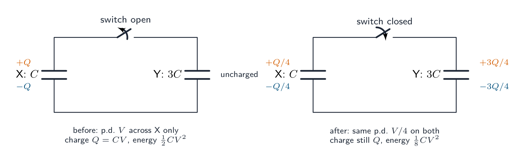
A fully charged capacitor X (capacitance $C$, p.d. $V$, charge $Q = CV$) is disconnected from its supply and connected across an uncharged capacitor Y of capacitance $3C$. Charge flows until the two p.d.s are equal. Two principles settle everything:

1. Charge is conserved. The total charge is still $Q$, now spread over a parallel pair of total capacitance $4C$, so the common p.d. is $V' = Q/(4C) = V/4$. X keeps $Q/4$ and Y takes $3Q/4$ (charge in the ratio of the capacitances, since the p.d. is the same).
2. Energy is not conserved. Before: $\tfrac{1}{2} C V^{2}$. After: $\tfrac{1}{2}(4C)(V/4)^{2} = \tfrac{1}{8} C V^{2}$. Three-quarters of the energy has gone: it is dissipated 耗散 as heat in the connecting wires (and as a spark or electromagnetic radiation) while the charge moves, however small the resistance.

Worked example. A $220\ \mu\text{F}$ capacitor charged to $9.0\ \text{V}$ is connected across an uncharged $440\ \mu\text{F}$ capacitor. Find the final p.d. and the energy lost.

$Q = CV = (220 \times 10^{-6})(9.0) = 1.98 \times 10^{-3}\ \text{C}$; total capacitance $660\ \mu\text{F}$, so $V' = 1.98 \times 10^{-3}/(660 \times 10^{-6}) = 3.0\ \text{V}$. Energy before: $\tfrac{1}{2}(220 \times 10^{-6})(9.0)^{2} = 8.9 \times 10^{-3}\ \text{J}$; after: $\tfrac{1}{2}(660 \times 10^{-6})(3.0)^{2} = 3.0 \times 10^{-3}\ \text{J}$; lost: $5.9 \times 10^{-3}\ \text{J}$, two-thirds of the original. A capacitor connected to another of capacitance $kC$ always loses the fraction $k/(k+1)$.

A capacitor $C$ charged to $V_{0}$ is connected through a switch to a resistor 电阻器 of resistance 电阻 $R$. When the switch closes at $t = 0$, the capacitor discharges.

Setting up the equation

By Kirchhoff's second law 基尔霍夫第二定律 around the loop, $V_{C} = V_{R}$. Using $V_{C} = Q/C$, $V_{R} = IR$ and $I = -dQ/dt$:

This is solved by an exponential decay 指数衰减 with time constant $RC$.

Discharge equations

Charge $Q$, p.d. $V$ and current $I$ all decay exponentially with the same time constant:

with $I_{0} = V_{0}/R$.

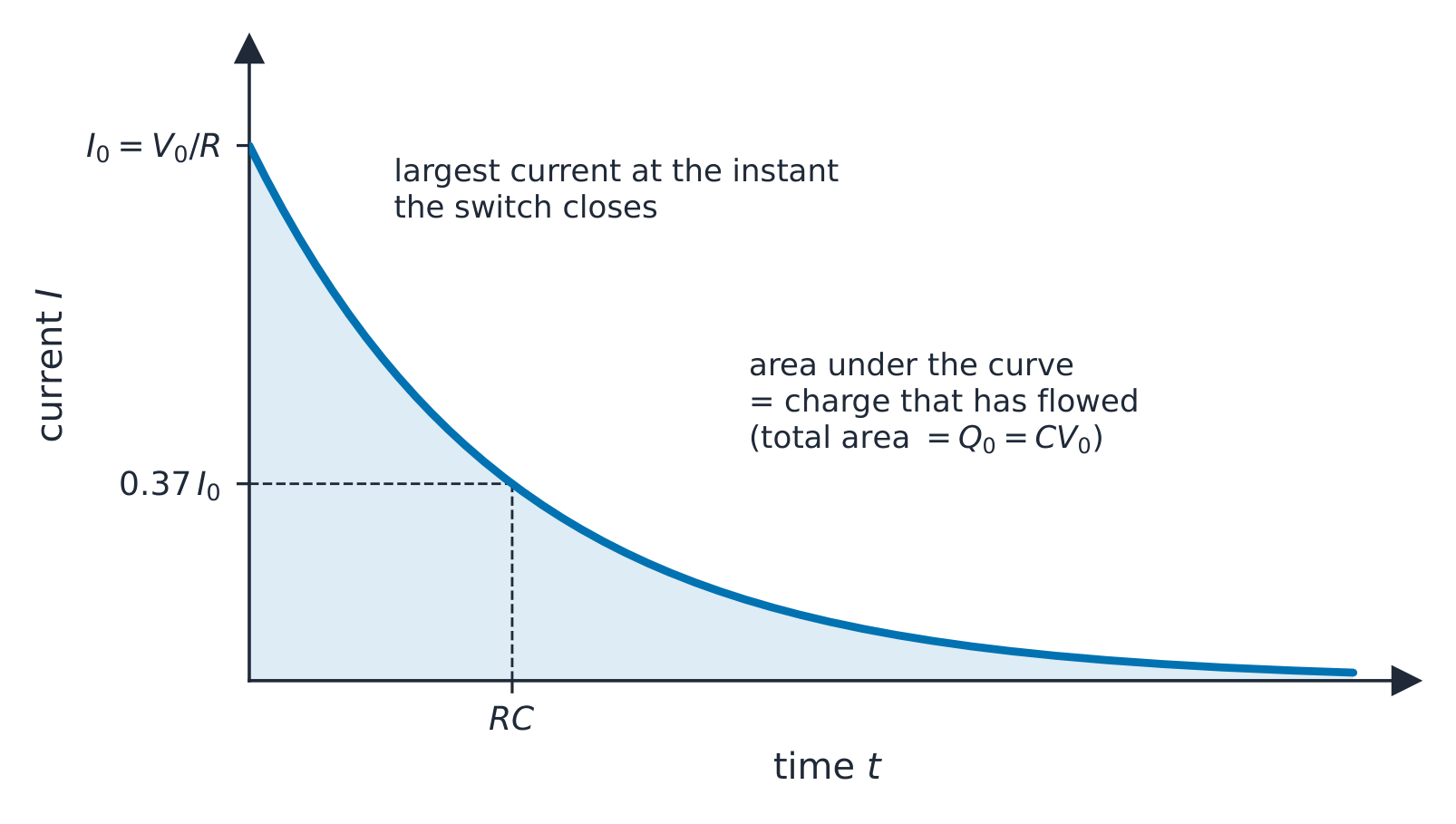
Reading the three graphs. All three curves have the same shape and the same time constant, so one measurement of $\tau$ from any of them gives $RC$. The current is largest the instant the switch closes, $I_{0} = V_{0}/R$, because the full p.d. $V_{0}$ is then across the resistor; it falls as the p.d. falls. The area under the $I$–$t$ graph is the charge that has flowed, so the total area is $Q_{0} = CV_{0}$, and the charge that flows in the first time constant is $Q_{0}(1 - e^{-1}) = 0.63\,Q_{0}$. The gradient of the $Q$–$t$ graph is $-I$: steepest at the start, flattening as the current dies away. (During charging through a resistor the current has the same decaying shape, while $V$ and $Q$ rise as $V_{0}(1 - e^{-t/RC})$, the mirror image of the discharge curve.)

Time constant

is the time constant 时间常数 (in seconds: $\Omega \cdot \text{F} = \text{s}$). It is the time for a decaying quantity to fall to $1/e \approx 0.37$ (about 37%) of its starting value. After $2\tau$ it is at about 13.5%; after $5\tau$, below 1%.

Worked example. A $100\ \mu\text{F}$ capacitor charged to $12\ \text{V}$ is discharged through a $47\ \text{k}\Omega$ resistor. Find the time constant and the voltage after one time constant.

After one time constant the voltage falls to $1/e$ of its start: $V = 12 \times 0.37 \approx 4.4\ \text{V}$.

Worked example. A $470\ \mu\text{F}$ capacitor is charged to $24\ \text{V}$ and then discharged through a $5.6\ \text{k}\Omega$ resistor. Find (a) the initial charge and energy, (b) the time constant and the initial current, (c) the p.d. after $4.0\ \text{s}$, (d) the time for the p.d. to fall to $6.0\ \text{V}$.

(a) $Q_{0} = CV_{0} = (470 \times 10^{-6})(24) = 1.1 \times 10^{-2}\ \text{C}$; $W = \tfrac{1}{2}CV_{0}^{2} = \tfrac{1}{2}(470 \times 10^{-6})(24)^{2} = 0.135\ \text{J}$. (b) $\tau = RC = (5.6 \times 10^{3})(470 \times 10^{-6}) = 2.6\ \text{s}$; $I_{0} = V_{0}/R = 24/5600 = 4.3\ \text{mA}$. (c) $V = V_{0} e^{-t/RC} = 24\, e^{-4.0/2.63} = 24 \times 0.219 = 5.3\ \text{V}$. (d) Rearrange with logarithms: $t = -RC \ln(V/V_{0}) = -2.63 \ln(6.0/24) = 2.63 \times 1.386 = 3.6\ \text{s}$.

Keep the time constant unrounded ($2.632\ \text{s}$) inside the calculation and round only the answers. The rearrangement in (d) is the one most often asked and most often botched: $\ln(V/V_{0})$ is negative, so $t$ comes out positive.

Worked example. From a discharge graph, the p.d. across a $2200\ \mu\text{F}$ capacitor falls from $6.0\ \text{V}$ to $2.2\ \text{V}$ in $4.5\ \text{s}$. Find the resistance of the resistor.

$2.2/6.0 = 0.367 \approx 1/e$, so $4.5\ \text{s}$ is one time constant: $R = \tau/C = 4.5/(2200 \times 10^{-6}) = 2.0 \times 10^{3}\ \Omega$. If the fall is not to $1/e$, use $RC = -t/\ln(V/V_{0})$; the answer is the same either way.

To find $\tau$ from a curve: read the time to fall to $1/e$ of the start. Or take logs: $\ln(V/V_{0}) = -t/(RC)$, so a plot of $\ln V$ against $t$ is a straight line with gradient $-1/(RC)$.

Using the logarithmic graph. In an experiment, plot $\ln V$ (or $\ln I$) on the $y$-axis against $t$. The points should lie on a straight line: its gradient is $-1/(RC)$, so $RC = -1/\text{gradient}$, and its intercept 截距 on the $\ln V$ axis is $\ln V_{0}$. A straight line is the test that the decay really is exponential; a curve means it is not. Take the gradient from two points far apart on the best-fit line, not from two data points, and quote $RC$ in seconds.

Reading graphs during discharge

• $Q$ against $V_{C}$: since $Q = C V$ always, this is a straight line through the origin with gradient $C$. Discharge moves the point from $(V_{0}, Q_{0})$ down to $(0,0)$.
• $I$ against $V_{C}$: since $I = V_{C}/R$, this is a straight line through the origin with gradient $1/R$, so you can find $R$.

Common exam questions

Given a discharge curve $V(t)$ or $Q(t)$:

• read the start value $V_{0}$ or $Q_{0}$ at $t = 0$.
• read the time to fall to $V_{0}/e$ → time constant $\tau = RC$.
• given $R$, find $C = \tau / R$ (or the other way round).
• predict a later value with the exponential formula.

A capacitor as a smoothing component

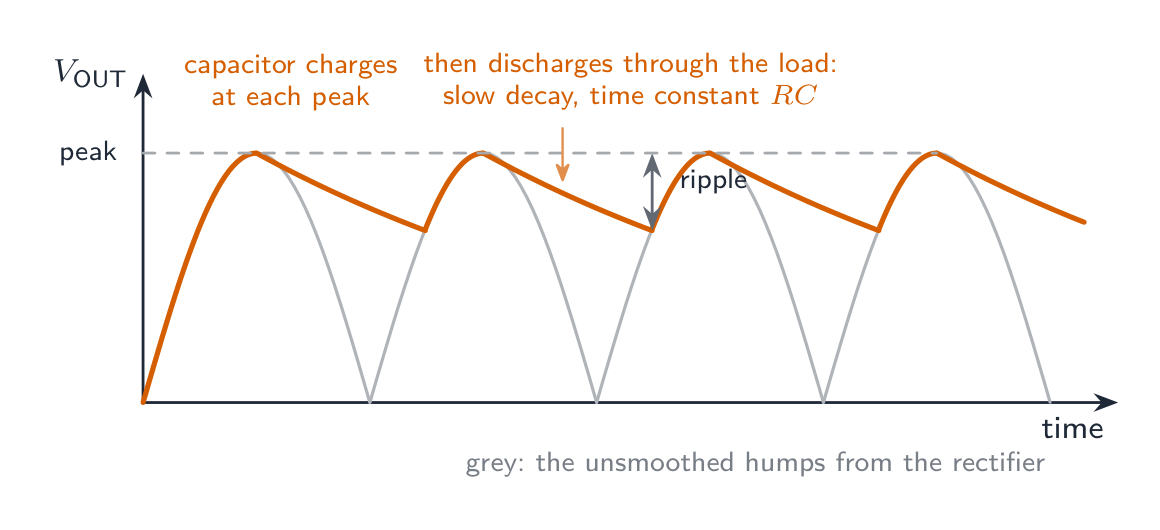
A rectifier 整流器 (Topic 21) turns an alternating voltage into a series of positive humps. A capacitor connected across the load smooths them. Near each peak 峰值 the diodes conduct and the capacitor charges to the peak voltage; as the supply voltage falls away the diodes stop conducting and the capacitor discharges through the load resistor, holding the output up until the next hump rises above it and recharges the capacitor. The output therefore falls only a little between peaks; the rise and fall that remains is the ripple 纹波.

How much it falls depends on the time constant of the discharge, $RC$, compared with the time between peaks. A larger capacitance, or a larger load resistance (a smaller load current), gives a larger $RC$, a slower decay and a smaller ripple; a heavily loaded supply (small $R$) has a larger ripple. Asked to sketch the smoothed output, draw it touching each peak, decaying slightly between them, and never falling to zero.

A definition question is marked against fixed wording. Learn these exactly, and give one answer only.

• $C = Q/V$ defines capacitance; for an isolated sphere $C = 4\pi\varepsilon_{0} r$. Energy stored $W = \tfrac{1}{2}QV = \tfrac{1}{2}CV^{2} = Q^{2}/2C$: pick the form that uses what you know, and remember that energy is not proportional to charge.
• Combine capacitors the opposite way to resistors (parallel add, series reciprocal), and reduce a network one step at a time.
• Charge sharing: charge is conserved, energy is not. Find the common p.d. from the total charge and the total capacitance first, then the energies.
• Discharge: $x = x_{0} e^{-t/RC}$ for $Q$, $V$ and $I$ alike; $t = -RC \ln(x/x_{0})$; $\tau = RC$ is in seconds ($\Omega \cdot \text{F} = \text{s}$) and is the time to fall to $37\%$, not to zero.
• Graphs: the initial current is $V_{0}/R$; the area under $I$–$t$ is charge; the gradient of $Q$–$t$ is $-I$; $\ln V$ against $t$ is a straight line of gradient $-1/(RC)$ and intercept $\ln V_{0}$.
• Convert $\mu\text{F}$ and $\text{k}\Omega$ before multiplying: $\text{k}\Omega \times \mu\text{F}$ gives milliseconds, not seconds.

Common mistakes

• Defining capacitance as "the charge stored" or "the charge on both plates". It is the charge on one plate per unit p.d. between the plates.
• Adding capacitors in series as if they were resistors, or forgetting to invert the reciprocal sum at the end.
• After charge sharing, using the supply voltage in $\tfrac{1}{2}CV^{2}$ instead of the new common p.d., or claiming the energy is conserved.
• Drawing the discharge current starting from zero. It starts at its largest value, $V_{0}/R$.
• Treating $\tau$ as the time to discharge completely; after $5\tau$ about $1\%$ remains.
• Dropping the minus sign in $t = -RC \ln(V/V_{0})$ and reporting a negative time.
• Finding the extra energy on raising the p.d. from the extra charge alone: subtract two areas (or two $\tfrac{1}{2}CV^{2}$ values).
• Sketching a smoothed output that falls to zero between peaks, or saying a larger load resistance gives a larger ripple.