Skip to content · ⁨الانتقال إلى المحتوى⁩

National Income and Price Determination · ⁨الدخل الوطني وتحديد الأسعار⁩

AP Macroeconomics · ⁨الاقتصاد الكلي (AP)⁩ · Topic 3 · ⁨الموضوع 3⁩

Video lesson for this topic · ⁨درس فيديو لهذا الموضوع⁩ Open the video page · ⁨افتح صفحة الفيديو⁩
8:50

الدخل الوطني وتحديد الأسعار

حكومة تنفق عشرة مليارات دولار على سكك حديد جديدة. كم يرتفع إنتاج البلاد؟ ليس عشرة مليارات. يمكن أن يرتفع بخمسين مليارًا. المال المنفق بواسطة…

English narration · English + 中文 subtitles burned in · ⁨سرد باللغة الإنجليزية · ترجمة مدمجة بالإنجليزية + الصينية⁩

3.1

Aggregate Demand · ⁨الطلب الكلي⁩

Syllabus · ⁨المنهج⁩
English

Enduring Understanding (MOD-2): Economists use the aggregate demand–aggregate supply model to represent the relationship between the price level and aggregate output in an economy and to illustrate how output, employment, and the price level respond to macroeconomic shocks.

Learning Objective MOD-2.A: a. Define (using graphs as appropriate) the aggregate demand (AD) curve. b. Explain (using graphs as appropriate) the slope of the AD curve and its determinants.

  • MOD-2.A.1 The aggregate demand (AD) curve describes the relationship between the price level and the quantity of goods and services demanded by households (consumption), firms (investment), government (government spending), and the rest of the world (net exports).
  • MOD-2.A.2 The negative slope of the AD curve is explained by the real wealth effect, the interest rate effect, and the exchange rate effect. [See EK MKT-3.A.1]
  • MOD-2.A.3 Any change in the components of aggregate demand (consumption, investment, government spending, or net exports) that is not due to changes in the price level leads to a shift of the AD curve.
العربية

فهم دائم (MOD-2): يستخدم الاقتصاديون نموذج الطلب الكلي والعرض الكلي لتمثيل العلاقة بين المستوى العام للأسعار والإنتاج الكلي في اقتصاد ما، ولتوضيح كيف تستجيب الإنتاجية والتوظيف والمستوى العام للأسعار للصدمات الكلية.

هدف التعلم MOD-2.A: أ. عرّف (باستخدام الرسوم البيانية عند الحاجة) منحنى الطلب الكلي (AD). ب. اشرح (باستخدام الرسوم البيانية عند الحاجة) ميل منحنى الطلب الكلي ومحدداته.

  • MOD-2.A.1 يصف منحنى الطلب الكلي (AD) العلاقة بين المستوى العام للأسعار والكمية المطلوبة من السلع والخدمات من قبل الأسر (الاستهلاك)، والشركات (الاستثمار)، والحكومة (الإنفاق الحكومي)، وبقية العالم (التصديرات الصافية).
  • MOD-2.A.2 يُفسر الميل السالب لمنحنى الطلب الكلي بتأثير الثروة الحقيقية، وتأثير سعر الفائدة، وتأثير سعر الصرف. [انظر EK MKT-3.A.1]
  • MOD-2.A.3 أي تغيير في مكونات الطلب الكلي (الاستهلاك، الاستثمار، الإنفاق الحكومي، أو التصديرات الصافية) الذي لا ينتج عن تغيرات في المستوى العام للأسعار يؤدي إلى إزاحة منحنى الطلب الكلي.
Source: College Board AP Course and Exam Description · ⁨المصدر: وصف دورة وامتحان College Board AP⁩

English
The AD–AS model: a demand shock

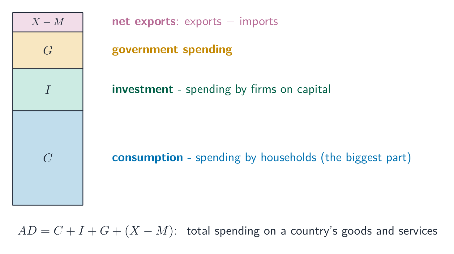
Aggregate demand (AD) 总需求 shows the total quantity of real output ($C+I+G+X_n$) buyers want at each price level 价格水平. It slopes downward for three reasons special to the whole economy:

  • the wealth effect 财富效应 (a higher price level shrinks the real value of money, so people buy less),
  • the interest-rate effect 利率效应 (a higher price level raises money demand and interest rates, cutting investment),
  • the net-export effect (a higher domestic price level makes exports dearer and imports cheaper).

A change in the price level is a movement along AD. AD shifts when any component of $C+I+G+X_n$ changes for another reason – consumer confidence, business expectations, government spending, taxes, or foreign incomes.

العربية
أفق مدينة: الناتج الوطني والطلب الكلي يعكسان الإنفاق على مستوى الاقتصاد
نموذج AD–AS: صدمة الطلب

الطلب الكلي (AD) يظهر إجمالي كمية الإنتاج الحقيقي ($C+I+G+X_n$) التي يريد المشترون الحصول عليها عند كل مستوى أسعار. ينحدر لأسفل لثلاثة أسباب خاصة بالاقتصاد ككل:

الطلب الكلي هو إجمالي الإنفاق: الاستهلاك، الاستثمار، الحكومة، والتصدير الصافي
الطلب الكلي هو إجمالي الإنفاق: الاستهلاك، الاستثمار، الحكومة، والصادرات الصافية
  • تأثير الثروة (ارتفاع مستوى الأسعار يقلل القيمة الحقيقية للنقود، مما يجعل الناس يشترون أقل)،
  • تأثير أسعار الفائدة (ارتفاع مستوى الأسعار يزيد الطلب على النقود وأسعار الفائدة، مما يقلل الاستثمار)،
  • تأثير الصادرات الصافية (ارتفاع مستوى الأسعار المحلي يجعل الصادرات أغلى والواردات أرخص).

التغير في مستوى الأسعار هو حركة على طول منحنى AD. وينزاح منحنى AD عندما يتغير أي مكون من $C+I+G+X_n$ لسبب آخر – مثل ثقة المستهلكين، وتوقعات الشركات، أو الإنفاق الحكومي، أو الضرائب، أو دخول الدول الأخرى.

3.2

The Spending and Tax Multipliers · ⁨مضاعف الإنفاق والضرائب⁩

Syllabus · ⁨المنهج⁩
English

Enduring Understanding (MOD-2): Economists use the aggregate demand–aggregate supply model to represent the relationship between the price level and aggregate output in an economy and to illustrate how output, employment, and the price level respond to macroeconomic shocks.

Learning Objective MOD-2.B: a. Define the expenditure multiplier, the tax multiplier, the marginal propensity to consume, and the marginal propensity to save. b. Explain how changes in spending and taxes lead to changes in real GDP. c. Calculate how changes in spending and taxes lead to changes in real GDP.

  • MOD-2.B.1 A $\$1$ change to autonomous expenditures leads to further changes in total expenditures and total output.
  • MOD-2.B.2 The expenditure multiplier quantifies the size of the change in aggregate demand as a result of a change in any of the components of aggregate demand.
  • MOD-2.B.3 The tax multiplier quantifies the size of the change in aggregate demand as a result of a change in taxes.
  • MOD-2.B.4 The expenditure multiplier and tax multiplier depend on the marginal propensity to consume.
  • MOD-2.B.5 The marginal propensity to consume is the change in consumer spending divided by the change in disposable income. The sum of the marginal propensity to consume and marginal propensity to save is equal to one.
العربية

فهم دائم (MOD-2): يستخدم الاقتصاديون نموذج الطلب الكلي والعرض الكلي لتمثيل العلاقة بين المستوى العام للأسعار والإنتاج الكلي في اقتصاد ما، ولتوضيح كيف تستجيب الإنتاجية والتوظيف والمستوى العام للأسعار للصدمات الكلية.

هدف التعلم MOD-2.B: أ. عرّف مضاعف الإنفاق، ومضاعف الضرائب، والميل الحدي للاستهلاك، والميل الحدي للادخار. ب. اشرح كيف تؤدي التغيرات في الإنفاق والضرائب إلى تغييرات في الناتج المحلي الإجمالي الحقيقي. ج. احسب كيف تؤدي التغيرات في الإنفاق والضرائب إلى تغييرات في الناتج المحلي الإجمالي الحقيقي.

  • MOD-2.B.1 أي تغيير $\$1$ في الإنفاق المستقل يؤدي إلى تغييرات إضافية في إجمالي الإنفاق وإجمالي الإنتاج.
  • MOD-2.B.2 يقيس مضاعف الإنفاق حجم التغير في الطلب الكلي كنتيجة لتغير في أي من مكونات الطلب الكلي.
  • MOD-2.B.3 يقيس مضاعف الضرائب حجم التغير في الطلب الكلي كنتيجة لتغير في الضرائب.
  • MOD-2.B.4 يعتمد مضاعف الإنفاق ومضاعف الضرائب على الميل الحدي للاستهلاك.
  • MOD-2.B.5 الميل الحدي للاستهلاك هو التغير في إنفاق المستهلك مقسومًا على التغير في الدخل المتاح. مجموع الميل الحدي للاستهلاك والميل الحدي للادخار يساوي واحدًا.

Source: College Board AP Course and Exam Description · ⁨المصدر: وصف دورة وامتحان College Board AP⁩

English
The spending multiplier

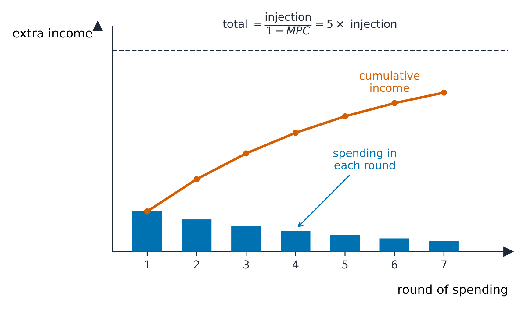
A change in spending sets off further rounds of spending, so the final change in GDP is larger than the initial change – the multiplier effect 乘数效应. It depends on the marginal propensity to consume 边际消费倾向 (MPC), the fraction of extra income that is spent (the rest is the marginal propensity to save 边际储蓄倾向, MPS, with $MPC+MPS=1$):

$$\text{spending multiplier}=\frac{1}{1-MPC}=\frac{1}{MPS}.$$

A tax cut works through the multiplier too, but more weakly, because part of the tax cut is saved:

$$\text{tax multiplier}=-\frac{MPC}{1-MPC}=-\frac{MPC}{MPS}.$$

The tax multiplier is smaller in size and negative (a tax cut raises GDP; a tax rise lowers it). Total change in GDP $=$ (multiplier) $\times$ (initial change).

Worked example. If $MPC=0.8$, the spending multiplier is $\dfrac{1}{1-0.8}=5$, so a $\$10$ billion rise in government spending lifts real GDP by $5\times\$10=\$50$ billion. The tax multiplier is $-\dfrac{0.8}{0.2}=-4$, so a $\$10$ billion tax cut raises GDP by only $\$40$ billion – weaker, because part of the tax cut is saved.

Exam skill: compute both multipliers from the MPC and find the resulting change in real GDP – an almost-guaranteed calculation.

العربية
مضاعف الإنفاق

يُحدث التغير في الإنفاق دورات إضافية من الإنفاق، لذا يكون التغير النهائي في الناتج المحلي الإجمالي أكبر من التغير الأولي – وهو ما يُعرف بـتأثير المضاعف. ويعتمد هذا على الميل الهامشي للاستهلاك (MPC)، وهو الجزء الإضافي من الدخل الذي يُنفق (والباقي هو الميل الهامشي للادخار، MPS، مع $MPC+MPS=1$):

حقنة واحدة تتضاعف لتصبح ارتفاعًا كليًا أكبر في الدخل
$$\text{spending multiplier}=\frac{1}{1-MPC}=\frac{1}{MPS}.$$

يعمل تخفيض الضرائب عبر المضاعف أيضًا، لكن بشكل أضعف، لأن جزءًا من تخفيض الضرائب يتم ادخاره:

$$\text{tax multiplier}=-\frac{MPC}{1-MPC}=-\frac{MPC}{MPS}.$$

مضاعف الضريبة أصغر حجمًا وسالب (تخفيض الضرائب يرفع الناتج المحلي الإجمالي؛ وزيادته يخفضه). التغير الكلي في الناتج المحلي الإجمالي $=$ (المضاعف) $\times$ (التغير الأولي).

مثال محلول. إذا $MPC=0.8$، فإن مضرب الإنفاق هو $\dfrac{1}{1-0.8}=5$، لذا فإن تخفيض ضريبي بمقدار $\$10$ billion rise in government spending lifts real GDP by $5\times\$10=\$50$ billion. The tax multiplier is $-\dfrac{0.8}{0.2}=-4$, so a $\$10$ مليار دولار يُقلل الناتج المحلي الإجمالي بمقدار $\$40$ مليار فقط – وهو تأثير أضعف، لأن جزءاً من التخفيض الضريبي يتم ادخاره.

مهارة الامتحان: احسب كلا المضاعفين من الميل الهامشي للاستهلاك وأوجد التغير الناتج في الناتج المحلي الإجمالي الحقيقي – وهي عملية حسابية مضمونة تقريبًا.

Explore · ⁨استكشف⁩

See the spending multiplier ripple out · ⁨شاهد مضاعف الإنفاق يتموج للخارج⁩

A dollar of new spending becomes someone's income, part of which they spend again — so the total effect is a multiple of the first injection, set by the marginal propensity to consume (MPC). · ⁨دولار من الإنفاق الجديد يصبح دخلاً لشخص ما، جزء منه يعيد إنفاقه مرة أخرى — لذا التأثير الكلي هو مضاعف للإدراج الأول، تحدده الميل الحدي للاستهلاك (MPC).⁩

3.3

Short-Run Aggregate Supply · ⁨العرض الإجمالي قصير الأجل⁩

Syllabus · ⁨المنهج⁩
English

Enduring Understanding (MOD-2): Economists use the aggregate demand–aggregate supply model to represent the relationship between the price level and aggregate output in an economy and to illustrate how output, employment, and the price level respond to macroeconomic shocks.

Learning Objective MOD-2.C: a. Define (using graphs as appropriate) the short-run aggregate supply (SRAS) curve. b. Explain (using graphs as appropriate) the slope of the SRAS curve and its determinants.

  • MOD-2.C.1 The short-run aggregate supply (SRAS) curve describes the relationship between the price level and the quantity of goods and services supplied in an economy.
  • MOD-2.C.2 The SRAS curve is upward-sloping because of sticky wages and prices. [See EK MOD-2.E.1]
  • MOD-2.C.3 Any factor that causes production costs to change, such as a change in inflationary expectations, will cause the SRAS curve to shift.

Learning Objective MOD-2.D: Explain (using graphs as appropriate) how movement along the SRAS curve implies a relationship between the price level (and inflation) and unemployment.

  • MOD-2.D.1 Moving along the SRAS curve, an increase in the price level is associated with an increase in output, which means employment must correspondingly rise. With the labor force held constant, unemployment will fall. So, there is a short-run trade-off between inflation and unemployment. [See EK MOD-3.A.1]
العربية

فهم دائم (MOD-2): يستخدم الاقتصاديون نموذج الطلب الكلي والعرض الكلي لتمثيل العلاقة بين المستوى العام للأسعار والإنتاج الكلي في اقتصاد ما، ولتوضيح كيف تستجيب الإنتاجية والتوظيف والمستوى العام للأسعار للصدمات الكلية.

هدف التعلم MOD-2.C: أ. عرّف (باستخدام الرسوم البيانية عند الحاجة) منحنى العرض الكلي قصير الأجل (SRAS). ب. اشرح (باستخدام الرسوم البيانية عند الحاجة) ميل منحنى العرض الكلي قصير الأجل ومحدداته.

  • MOD-2.C.1 يصف منحنى العرض الكلي قصير الأجل (SRAS) العلاقة بين المستوى العام للأسعار والكمية المعروضة من السلع والخدمات في اقتصاد ما.
  • MOD-2.C.2 يكون منحنى SRAS متجهًا للأعلى بسبب ثبات الأجور والأسعار. [انظر EK MOD-2.E.1]
  • MOD-2.C.3 أي عامل يسبب تغيرًا في تكاليف الإنتاج، مثل تغير في التوقعات التضخمية، سيؤدي إلى إزاحة منحنى العرض الكلي قصير الأجل.

هدف التعلم MOD-2.D: اشرح (باستخدام الرسوم البيانية عند الحاجة) كيف يشير التحرك على طول منحنى العرض الكلي قصير الأجل إلى وجود علاقة بين المستوى العام للأسعار (والتضخم) والبطالة.

  • MOD-2.D.1 مع التحرك على طول منحنى العرض الكلي قصير الأجل، يرتبط ارتفاع المستوى العام للأسعار بزيادة الإنتاج، مما يعني أنه يجب أن ترتفع العمالة بالتناظر. وبثبات القوى العاملة، سينخفض معدل البطالة. لذا، توجد مفاضلة قصيرة الأجل بين التضخم والبطالة. [انظر EK MOD-3.A.1]

Source: College Board AP Course and Exam Description · ⁨المصدر: وصف دورة وامتحان College Board AP⁩

English

Short-run aggregate supply (SRAS) 短期总供给 slopes upward: in the short run some input prices (especially nominal wages 名义工资) are sticky 粘性, so a higher output price level widens profit margins and firms produce more. SRAS shifts with input prices, productivity, taxes/subsidies on producers, and supply shocks (e.g. an oil-price change). A rise in input costs shifts SRAS left.

العربية
محطة طاقة وموقع صناعي: يعتمد العرض الإجمالي قصير الأجل على تكاليف الإنتاج

عرض إجمالي قصير الأجل (SRAS) يتجه للأعلى: ففي قصير الأجل تكون بعض أسعار المدخلات (خاصة الأجور الاسمية) لا مرنة، لذا يؤدي ارتفاع مستوى أسعار المخرجات إلى توسيع هوامش الربح وإنتاج الشركات أكثر. وينزاح عرض SRAS بسبب أسعار المدخلات، والإنتاجية، والضرائب/بدائل الإنتاج، وصدمة العرض (مثل تغير سعر النفط). يؤدي ارتفاع تكاليف المدخلات إلى انزاحة SRAS لليسار.

3.4

Long-Run Aggregate Supply · ⁨العرض الإجمالي طويل الأجل⁩

Syllabus · ⁨المنهج⁩
English

Enduring Understanding (MOD-2): Economists use the aggregate demand–aggregate supply model to represent the relationship between the price level and aggregate output in an economy and to illustrate how output, employment, and the price level respond to macroeconomic shocks.

Learning Objective MOD-2.E: Define (using graphs as appropriate) the short run and the long run.

  • MOD-2.E.1 In the long run all prices and wages are fully flexible, while in the short run some input prices are fixed. A consequence of flexible long-run prices and wages is the lack of a long-run trade-off between inflation and unemployment.

Learning Objective MOD-2.F: Define (using graphs as appropriate) the long-run aggregate supply (LRAS) curve.

  • MOD-2.F.1 The LRAS curve corresponds to the production possibilities curve (PPC) because they both represent maximum sustainable capacity. Maximum sustainable capacity is the total output an economic system will produce over a set period of time if all resources are fully employed. [See LO MOD-2.I]
  • MOD-2.F.2 The LRAS curve is vertical at the full-employment level of output because in the long run wages and prices fully adjust.
العربية

فهم دائم (MOD-2): يستخدم الاقتصاديون نموذج الطلب الكلي والعرض الكلي لتمثيل العلاقة بين المستوى العام للأسعار والإنتاج الكلي في اقتصاد ما، ولتوضيح كيف تستجيب الإنتاجية والتوظيف والمستوى العام للأسعار للصدمات الكلية.

هدف التعلم MOD-2.E: عرّف (باستخدام الرسوم البيانية عند الحاجة) المدى القصير والمدى الطويل.

  • MOD-2.E.1 في المدى الطويل تكون جميع الأسعار والأجور مرنة تمامًا، بينما في المدى القصير بعض أسعار المدخلات ثابتة. ومن نتائج مرونة الأسعار والأجور طويلة الأجل عدم وجود مفاضلة طويلة الأجل بين التضخم والبطالة.

هدف التعلم MOD-2.F: عرّف (باستخدام الرسوم البيانية عند الحاجة) منحنى العرض الكلي طويل الأجل (LRAS).

  • MOD-2.F.1 يتوافق منحنى LRAS مع منحنى إمكانيات الإنتاج (PPC) لأن كليهما يمثلان القدرة القصوى المستدامة. القدرة القصوى المستدامة هي إجمالي الإنتاج الذي سيقدمه النظام الاقتصادي خلال فترة زمنية محددة إذا تم توظيف جميع الموارد بالكامل. [انظر LO MOD-2.I]
  • MOD-2.F.2 يكون منحنى LRAS عموديًا عند مستوى التوظيف الكامل للإنتاج لأنه في المدى الطويل تتكيف الأجور والأسعار بالكامل.

Source: College Board AP Course and Exam Description · ⁨المصدر: وصف دورة وامتحان College Board AP⁩

English

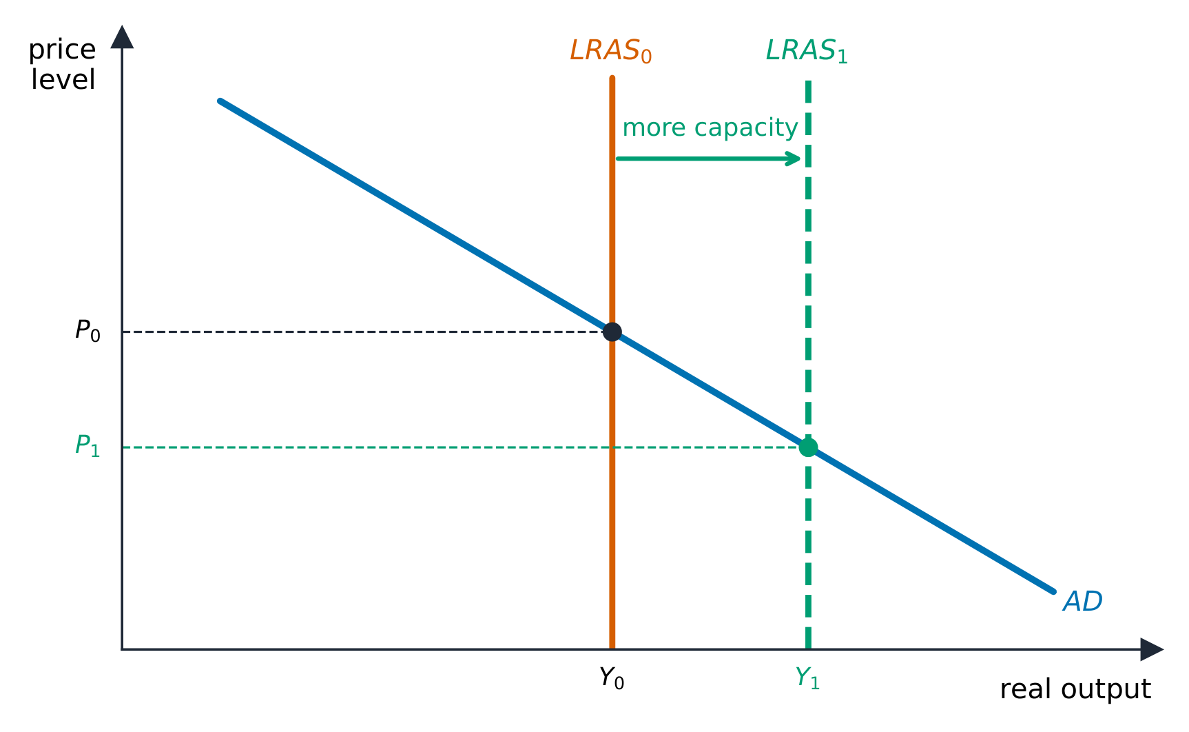
Long-run aggregate supply (LRAS) 长期总供给 is vertical at the economy's full-employment (potential) output 潜在产出 $Y_f$. In the long run all prices and wages are fully flexible (only in the short run are some input prices fixed), so output depends only on real factors – resources, technology, institutions – not the price level. LRAS shifts only with economic growth (more or better resources). LRAS corresponds to the production possibilities curve (PPC) 生产可能性曲线: both mark the economy's maximum sustainable capacity, so an outward LRAS shift and an outward PPC shift are the same event drawn two ways. The vertical LRAS is why, in the long run, demand policy changes prices, not output.

العربية

عرض إجمالي طويل الأجل (LRAS) يكون عموديًا عند الناتج الكامل للتوظيف (ناتج الإمكانات) $Y_f$. وفي طويل الأجل تكون جميع الأسعار والأجور مرنة تمامًا (تبقى بعض أسعار المدخلات ثابتة فقط في قصير الأجل)، لذا يعتمد الناتج فقط على العوامل الحقيقية – الموارد، والتكنولوجيا، والمؤسسات – وليس على مستوى الأسعار. ينزاح LRAS فقط مع النمو الاقتصادي (زيادة أو تحسين الموارد). يرتبط LRAS بـمنحنى إمكانيات الإنتاج (PPC): فكل منهما يشير إلى الحد الأقصى للاستدامة للإنتاج في الاقتصاد، لذا فإن انزاحة LRAS للخارج وانزاحة PPC للخارج هما نفس الحدث مُصوَّرين بطريقتين. ومن هنا يأتي سبب كون منحنى LRAS عموديًا، sehingga في طويل الأجل، تؤدي سياسات الطلب إلى تغيير الأسعار لا الناتج.

سياسة جانب العرض تنزح العرض الإجمالي طويل الأجل لليمين: زيادة في الناتج، انخفاض في الأسعار
3.5

Equilibrium in the AD-AS Model · ⁨التوازن في نموذج AD-AS⁩

Syllabus · ⁨المنهج⁩
English

Enduring Understanding (MOD-2): Economists use the aggregate demand–aggregate supply model to represent the relationship between the price level and aggregate output in an economy and to illustrate how output, employment, and the price level respond to macroeconomic shocks.

Learning Objective MOD-2.G: Explain (using graphs as appropriate) the short-run and long-run equilibrium price level and output level.

  • MOD-2.G.1 Short-run equilibrium occurs when the aggregate quantity of output demanded and the aggregate quantity of output supplied are equal—i.e., at the intersection of the AD and SRAS curves.
  • MOD-2.G.2 Long-run equilibrium occurs when the AD and SRAS curves intersect on the LRAS—i.e., at the full-employment level of real output.
  • MOD-2.G.3 The short-run equilibrium output can be at the full-employment level of output, above it, or below it, creating positive (i.e., inflationary) or negative (i.e., recessionary) output gaps.
العربية

فهم دائم (MOD-2): يستخدم الاقتصاديون نموذج الطلب الكلي والعرض الكلي لتمثيل العلاقة بين المستوى العام للأسعار والإنتاج الكلي في اقتصاد ما، ولتوضيح كيف تستجيب الإنتاجية والتوظيف والمستوى العام للأسعار للصدمات الكلية.

هدف التعلم MOD-2.G: اشرح (باستخدام الرسوم البيانية عند الحاجة) المستوى العام للأسعار ومستوى الإنتاج في التوازن قصير الأجل وطويل الأجل.

  • MOD-2.G.1 يحدث التوازن قصير الأجل عندما تتساوى الكمية الكلية للإنتاج المطلوبة والكمية الكلية للإنتاج المعروضة - أي عند تقاطع منحنَيي AD و SRAS.
  • MOD-2.G.2 يحدث التوازن طويل الأجل عندما يتقاطع منحني AD و SRAS على منحنى LRAS - أي عند مستوى التوظيف الكامل للإنتاج الحقيقي.
  • MOD-2.G.3 يمكن أن يكون إنتاج التوازن قصير الأجل عند مستوى التوظيف الكامل للإنتاج، أو فوقه، أو تحته، مما يخلق فجوات إنتاجية إيجابية (أي تضخمية) أو سالبة (أي ركودية).

Source: College Board AP Course and Exam Description · ⁨المصدر: وصف دورة وامتحان College Board AP⁩

English

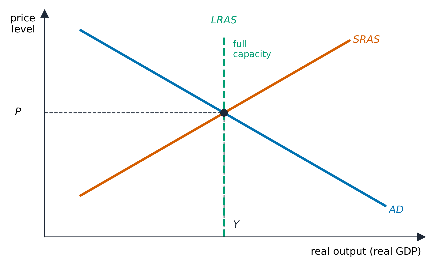
The economy settles where AD meets SRAS, fixing the equilibrium price level and real GDP. Comparing that output to $Y_f$ (the LRAS line) gives the economy's state:

  • output $: a recessionary gap 衰退缺口 (cyclical unemployment),
  • output $>Y_f$: an inflationary gap 通胀缺口 (overheating),
  • output $=Y_f$: long-run equilibrium.
العربية

يستقر الاقتصاد حيث يقابل AD منحنى SRAS، مما يحدد مستوى الأسعار المتوازن والناتج المحلي الإجمالي الحقيقي. ومقارنة هذا الناتج بـ $Y_f$ (خط LRAS) يعطي حالة الاقتصاد:

توازن ماكرواقتصادي حيث يقابل الطلب الإجمالي العرض الإجمالي
  • ناتج $: فجوة ركود (بطالة دورية)،
  • ناتج $>Y_f$: فجوة تضخمية (احتراق اقتصادي)،
  • ناتج $=Y_f$: توازن طويل الأجل.
Explore · ⁨استكشف⁩

Find equilibrium in the AD-AS model · ⁨جد التوازن في نموذج AD-AS⁩

Aggregate demand and aggregate supply cross at the economy's price level and real GDP. A demand or supply shock shifts a curve and moves the whole economy's output and prices. · ⁨الطلب الكلي والعرض الكلي يتقاطعان عند مستوى الأسعار والناتج المحلي الحقيقي للاقتصاد. صدمة طلب أو عرض تزاح منحنى وتحرك ناتج وأسعار الاقتصاد ككل.⁩

3.6

Short-Run Changes: Demand and Supply Shocks · ⁨التغيرات قصيرة الأجل: صدمات الطلب والعرض⁩

Syllabus · ⁨المنهج⁩
English

Enduring Understanding (MOD-2): Economists use the aggregate demand–aggregate supply model to represent the relationship between the price level and aggregate output in an economy and to illustrate how output, employment, and the price level respond to macroeconomic shocks.

Learning Objective MOD-2.H: Explain (using graphs as appropriate) the response of output, employment, and the price level to an aggregate demand or aggregate supply shock in the short run.

  • MOD-2.H.1 A positive (negative) shock in AD causes output, employment, and the price level to rise (fall) in the short run.
  • MOD-2.H.2 A positive (negative) shock in SRAS causes output and employment to rise (fall) and the price level to fall (rise) in the short run.
  • MOD-2.H.3 Inflation can be caused by changes in aggregate demand (demand-pull) or aggregate supply (cost-push).
العربية

فهم دائم (MOD-2): يستخدم الاقتصاديون نموذج الطلب الكلي والعرض الكلي لتمثيل العلاقة بين المستوى العام للأسعار والإنتاج الكلي في اقتصاد ما، ولتوضيح كيف تستجيب الإنتاجية والتوظيف والمستوى العام للأسعار للصدمات الكلية.

هدف التعلم MOD-2.H: اشرح (باستخدام الرسوم البيانية عند الحاجة) استجابة الإنتاج والتوظيف والمستوى العام للأسعار لصدمة الطلب الكلي أو العرض الكلي في المدى القصير.

  • MOD-2.H.1 يؤدي الصدمة الإيجابية (السلبية) في الطلب الكلي إلى ارتفاع (انخفاض) الإنتاج والوظائف ومستوى الأسعار على المدى القصير.
  • MOD-2.H.2 تؤدي الصدمة الإيجابية (السلبية) في عرض العمل الكلي قصير الأجل إلى ارتفاع (انخفاض) الإنتاج والوظائف وانخفاض (ارتفاع) مستوى الأسعار على المدى القصير.
  • MOD-2.H.3 يمكن أن يحدث التضخم نتيجة لتغيرات في الطلب الكلي (الطلب الدافع) أو العرض الكلي (الدفع التكلفة).

Source: College Board AP Course and Exam Description · ⁨المصدر: وصف دورة وامتحان College Board AP⁩

English
  • A demand shock shifts AD: a positive one (more spending) raises both price level and output (and lowers unemployment); a negative one lowers both.
  • A supply shock shifts SRAS: a negative one (higher input costs) raises the price level and lowers output at once – stagflation 滞胀 – the hardest case for policymakers, because fixing one worsens the other.
العربية
  • صدمة الطلب تُزوح منحنى AD: إيجابية (زيادة الإنفاق) ترفع كلًا من مستوى الأسعار والناتج (وتقلل البطالة)؛ وسلبية تخفض الاثنين معًا.
  • صدمة العرض تُزوح منحنى SRAS: سلبية (ارتفاع تكاليف المدخلات) ترفع مستوى الأسعار وتخفض الناتج في آن واحد – ركود تضخمي – وهو أصعب scenario للمشرعين، لأن إصلاح أحدهما ي worsens الآخر.
3.7

Long-Run Self-Adjustment · ⁨التصحيح الذاتي طويل الأجل⁩

Syllabus · ⁨المنهج⁩
English

Enduring Understanding (MOD-2): Economists use the aggregate demand–aggregate supply model to represent the relationship between the price level and aggregate output in an economy and to illustrate how output, employment, and the price level respond to macroeconomic shocks.

Learning Objective MOD-2.I: Explain (using graphs as appropriate) the response of output, employment, and the price level to an aggregate demand or aggregate supply shock in the long run.

  • MOD-2.I.1 In the long run, in the absence of government policy actions, flexible wages and prices will adjust to restore full employment and unemployment will revert to its natural rate after a shock to aggregate demand or short-run aggregate supply. [See EK MEA-1.E.2]
  • MOD-2.I.2 Shifts in the long-run aggregate supply curve indicate changes in the full-employment level of output and economic growth.
العربية

فهم دائم (MOD-2): يستخدم الاقتصاديون نموذج الطلب الكلي والعرض الكلي لتمثيل العلاقة بين المستوى العام للأسعار والإنتاج الكلي في اقتصاد ما، ولتوضيح كيف تستجيب الإنتاجية والتوظيف والمستوى العام للأسعار للصدمات الكلية.

هدف التعلم MOD-2.I: اشرح (باستخدام الرسوم البيانية عند الحاجة) استجابة الإنتاج والوظائف ومستوى الأسعار لصدمة الطلب الكلي أو العرض الكلي على المدى الطويل.

  • MOD-2.I.1 على المدى الطويل، وغياب إجراءات السياسة الحكومية، ستقوم الأجور والأسعار المرنة بالتكيف لاستعادة التوظيف الكامل وستعود البطالة إلى معدلها الطبيعي بعد صدمة في الطلب الكلي أو عرض العمل الكلي قصير الأجل. [راجع EK MEA-1.E.2]
  • MOD-2.I.2 تشير تحركات منحنى العرض الكلي طويل الأمد إلى تغيرات في مستوى التوظيف الكامل للإنتاج والنمو الاقتصادي.

Source: College Board AP Course and Exam Description · ⁨المصدر: وصف دورة وامتحان College Board AP⁩

English

Left alone, the economy self-corrects through flexible wages:

  • In a recessionary gap, high unemployment eventually pushes nominal wages down, shifting SRAS right until output returns to $Y_f$ at a lower price level.
  • In an inflationary gap, labor shortages push wages up, shifting SRAS left back to $Y_f$ at a higher price level.

The debate over how fast this happens is the case for (or against) active policy: self-adjustment is slow and painful, which is the argument for intervening.

العربية

مُتركًا لذاته، يصحح الاقتصاد نفسه تلقائيًا عبر مرونة الأجور:

  • في فجوة الركود، يؤدي البطالة المرتفعة في النهاية إلى انخفاض الأجور الاسمية، مما يُزوح SRAS ليمينًا حتى يعود الناتج إلى $Y_f$ عند مستوى أسعار أقل.
  • في الفجوة التضخمية، تؤدي نقص العمالة إلى ارتفاع الأجور، مما يُزوح SRAS يسارًا عائدًا إلى $Y_f$ عند مستوى أسعار أعلى.

النقاش حول سرعة حدوث ذلك هو جوهر جدلية سياسة التدخل: فالتصحيح الذاتي بطيء ومؤلم، وهو ما يُقدم كحجة للتدخل.

3.8

Fiscal Policy · ⁨السياسة المالية⁩

Syllabus · ⁨المنهج⁩
English

Enduring Understanding (POL-1): Fiscal and monetary policy have short-run effects on macroeconomic outcomes.

Learning Objective POL-1.A: a. Define fiscal policy and related terms. b. Explain (using graphs as appropriate) the short-run effects of a fiscal policy action. c. Calculate the short-run effects of a fiscal policy action.

  • POL-1.A.1 Governments implement fiscal policies to achieve macroeconomic goals, such as full employment.
  • POL-1.A.2 The tools of fiscal policy are government spending and taxes/transfers.
  • POL-1.A.3 Changes in government spending affect aggregate demand directly, and changes in taxes/transfers affect aggregate demand indirectly.
  • POL-1.A.4 The government spending multiplier is greater than the tax multiplier.
  • POL-1.A.5 Expansionary or contractionary fiscal policies are used to restore full employment when the economy is in a negative (i.e., recessionary) or positive (i.e., inflationary) output gap.
  • POL-1.A.6 Fiscal policy can influence aggregate demand, real output, and the price level. [See also EK MKT-5.E.2 for the effect on exchange rates.]
  • POL-1.A.7 The AD–AS model is used to demonstrate the short-run effects of fiscal policy.

Learning Objective POL-1.B: Define why there are lags to discretionary fiscal policy.

  • POL-1.B.1 In reality, there are lags to discretionary fiscal policy because of factors such as the time it takes to decide on and implement a policy action.
العربية

الفهم الدائم (POL-1): للسياسة المالية والنقدية تأثيرات قصيرة الأمد على النتائج الكلية للاقتصاد.

هدف التعلم POL-1.A: أ. عرّف السياسة المالية والمصطلحات ذات الصلة. ب. اشرح (باستخدام الرسوم البيانية عند الحاجة) التأثيرات قصيرة الأمد لإجراء سياسة مالية. ج. احسب التأثيرات قصيرة الأمد لإجراء سياسة مالية.

  • POL-1.A.1 تطبق الحكومات السياسات المالية لتحقيق أهداف كلية للاقتصاد، مثل التوظيف الكامل.
  • POL-1.A.2 أدوات السياسة المالية هي الإنفاق الحكومي والضرائب/التحويلات.
  • POL-1.A.3 تؤثر التغييرات في الإنفاق الحكومي مباشرة على الطلب الكلي، بينما تؤثر التغييرات في الضرائب/التحويلات على الطلب الكلي بشكل غير مباشر.
  • POL-1.A.4 مضاعف الإنفاق الحكومي أكبر من مضاعف الضرائب.
  • POL-1.A.5 تُستخدم السياسات المالية التوسعية أو الانقباضية لاستعادة التوظيف الكامل عندما يكون الاقتصاد في فجوة إنتاج سلبية (أي انكماشية) أو إيجابية (أي تضخمية).
  • POL-1.A.6 يمكن للسياسة المالية أن تؤثر على الطلب الكلي والإنتاج الحقيقي ومستوى الأسعار. [راجع أيضًا EK MKT-5.E.2 فيما يتعلق بتأثيرها على أسعار الصرف.]
  • POL-1.A.7 يُستخدم نموذج الطلب الكلي وعرض العمل الكلي لإظهار التأثيرات قصيرة الأمد للسياسة المالية.

هدف التعلم POL-1.B: عرّف أسباب وجود تأخر في السياسة المالية الاختيارية.

  • POL-1.B.1 في الواقع، هناك تأخر في السياسة المالية الاختيارية بسبب عوامل مثل الوقت المستغرق لاتخاذ قرار بشأن تنفيذ إجراء سياسي.

Source: College Board AP Course and Exam Description · ⁨المصدر: وصف دورة وامتحان College Board AP⁩

English

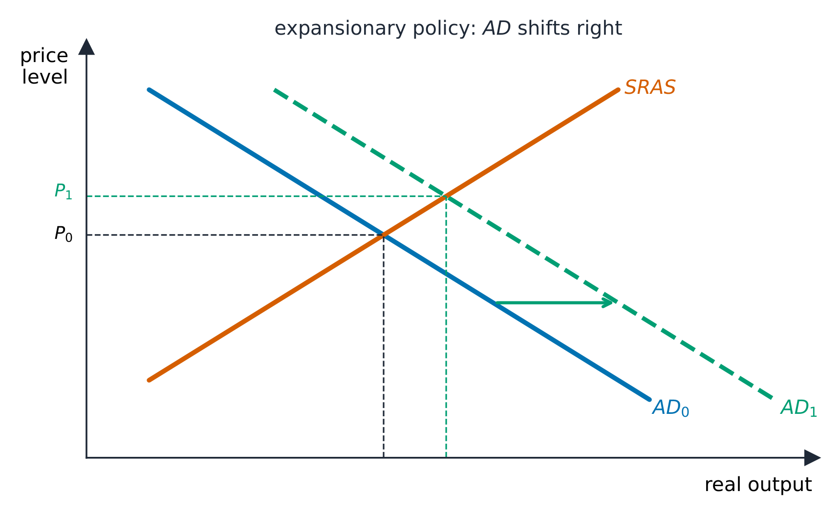
Fiscal policy 财政政策 is the government's use of spending and taxes to shift AD:

  • Expansionary 扩张性 (more spending or lower taxes) shifts AD right to close a recessionary gap.
  • Contractionary 紧缩性 (less spending or higher taxes) shifts AD left to close an inflationary gap.

Size the policy with the multipliers: to close a gap of a given size, the required change in spending is (gap) $\div$ (spending multiplier). Limits include time lags, crowding out (below), and political difficulty.

Worked example. An economy has a $\$100$ billion recessionary gap and $MPC=0.75$ (spending multiplier $=\dfrac{1}{0.25}=4$). To close it, the government must raise spending by $\dfrac{\$100\text{ billion}}{4}=\$25$ billion. Using a tax cut instead (tax multiplier $-3$) would require a larger $\dfrac{100}{3}\approx\$33$ billion cut.

Exam skill: you must draw the correctly labeled AD-AS graph, identify the gap, prescribe the right fiscal action and its direction, and often calculate the exact spending or tax change needed.

العربية

السياسة المالية هي استخدام الحكومة لـالإنفاق والضرائب لتحريك منحنى AD:

السياسة المالية التوسعية تُزوح منحنى AD لليمين، رافعةً الناتج والأسعار
  • توسعية (زيادة الإنفاق أو خفض الضرائب) تُزوح منحنى AD ليمينًا لإغلاق فجوة الركود.
  • انقباضية (تقليل الإنفاق أو رفع الضرائب) تُزوح منحنى AD ليسارًا لإغلاق فجوة التضخم.

تحديد حجم السياسة بالمضاعفات: لإغلاق فجوة بحجم معين، التغير المطلوب في الإنفاق هو (الفجوة) $\div$ (مضاعف الإنفاق). وتشمل الحدود التأخر الزمني، وإزاحة الموارد (أسفل)، وصعوبة سياسية.

مثال محلول. اقتصاد لديه $\$100$ billion recessionary gap and $MPC=0.75$ (spending multiplier $=\dfrac{1}{0.25}=4$). To close it, the government must raise spending by $\dfrac{\$100\text{ billion}}{4}=\$25$ billion. Using a tax cut instead (tax multiplier $-3$) would require a larger $\dfrac{100}{3}\approx\$33$ مليار تخفيض.

مهارة الامتحان: يجب أن ترسم رسمًا بيانيًا لـ AD-AS مع تسميات صحيحة، وتحديد الفجوة، واقتراح الإجراء المالي الصحيح واتجاهه، وغالبًا ما تحسب التغير الدقيق في الإنفاق أو الضرائب المطلوب.

Vocabulary · ⁨مفردات⁩ Train · ⁨تدريب⁩
English العربية
Aggregate demand (AD)/ˈæɡrɪɡeɪt dɪˈmænd/ الإجماع الكلي (AD)
price level/praɪs ˈlevl/ مستوى الأسعار
wealth effect/welθ ɪˈfekt/ تأثير الثروة
interest-rate effect/ˈɪntrest reɪt ɪˈfekt/ تأثير معدل الفائدة
multiplier effect/ˌmʌltɪˈplaɪə ɪˈfekt/ تأثير المضاعف
marginal propensity to consume/ˈmɑːdʒɪnl prəˈpensɪti tə kənˈsjuːm/ الميل الهامشي للاستهلاك
marginal propensity to save/ˈmɑːdʒɪnl prəˈpensɪti tə seɪv/ الميل الحدي للادخار
Short-run aggregate supply (SRAS)/ʃɔːt rʌn ˈæɡrɪɡeɪt səˈplaɪ/ الإجماع الكلي للعرض القصير (SRAS)
nominal wages/ˈnɒmɪnl ˈweɪdʒɪz/ الأجور الاسمية
sticky/ˈstɪki/ لزجة
Long-run aggregate supply (LRAS)/lɒŋ rʌn ˈæɡrɪɡeɪt səˈplaɪ/ الإجماع الكلي للعرض الطويل (LRAS)
full-employment (potential) output/fʊl emˈplɔɪmənt ˈaʊtpʊt/ إنتاج التشغيل الكامل (الإمكانات)
production possibilities curve (PPC)/prəˈdʌkʃn ˌpɒsəˈbɪlɪtiz kɜːv/ منحنى إمكانيات الإنتاج (PPC)
recessionary gap/rɪˈseʃənəri ɡæp/ فجوة انكماشية
inflationary gap/ɪnˈfleɪʃənəri ɡæp/ فجوة تضخمية
stagflation/stæɡˈfleɪʃn/ التضخم الركودي
Fiscal policy/ˈfɪskl ˈpɒlɪsi/ السياسة المالية
Expansionary/ekˈspænʃənəri/ توسعي
Contractionary/kənˈtrækʃənəri/ انقباضي
Automatic stabilizers/ˌɔːtəˈmætɪk ˈsteɪbəlaɪzəz/ المثبتات التلقائية
discretionary/dɪˈskreʃənəri/ اختياري
3.9

Automatic Stabilizers · ⁨Stabilizers التلقائية⁩

Syllabus · ⁨المنهج⁩
English

Enduring Understanding (POL-1): Fiscal and monetary policy have short-run effects on macroeconomic outcomes.

Learning Objective POL-1.C: a. Define automatic stabilizers. b. Explain how automatic stabilizers moderate business cycles.

  • POL-1.C.1 Automatic stabilizers support the economy during recessions and help prevent the economy from being overheated during expansionary periods.
  • POL-1.C.2 Tax revenues decrease automatically as GDP falls, preventing consumption and the economy from falling further.
  • POL-1.C.3 Tax revenues increase automatically as GDP rises, slowing consumption and preventing the economy from overheating.
  • POL-1.C.4 Government policies, institutions, or agencies may also have social service programs whose transfer payments act as automatic stabilizers.
العربية

الفهم الدائم (POL-1): للسياسة المالية والنقدية تأثيرات قصيرة الأمد على النتائج الكلية للاقتصاد.

هدف التعلم POL-1.C: أ. عرّف المستثباتات التلقائية. ب. اشرح كيف تخفف المستثباتات التلقائية من دورات الأعمال.

  • POL-1.C.1 تدعم المستثباتات التلقائية الاقتصاد أثناء فترات الركود وتساعد في منع الاقتصاد من السخونة الزائدة خلال فترات التوسع.
  • POL-1.C.2 تنخفض إيرادات الضرائب تلقائياً مع انخفاض الناتج المحلي الإجمالي، مما يمنع استهلاك المستهلكين والاقتصاد من الانخفاض أكثر.
  • POL-1.C.3 تزداد إيرادات الضرائب تلقائياً مع ارتفاع الناتج المحلي الإجمالي، مما يبطئ الاستهلاك ويمنع الاقتصاد من السخونة الزائدة.
  • POL-1.C.4 قد تمتلك سياسات الحكومة أو مؤسساتها أو وكالاتها أيضاً برامج خدمات اجتماعية تعمل فيها مدفوعات التحويل كمستثباتات تلقائية.

Source: College Board AP Course and Exam Description · ⁨المصدر: وصف دورة وامتحان College Board AP⁩

English

Automatic stabilizers 自动稳定器 are features that dampen the cycle without new legislation. In a downturn, progressive taxes collect less and transfer payments (unemployment benefits, welfare) rise automatically – cushioning incomes and spending; in a boom they do the reverse. They soften the cycle and act instantly, avoiding the lags of discretionary 相机抉择 policy.

العربية

Stabilizers التلقائية هي خصائص تخفف من دورات الاقتصاد بدون تشريعات جديدة. في حالة الركود، تجمع ضرائب متدرجة أقل وترتفع المدفوعات الانتقالية (مثل إعانات البطالة والرفاهية) تلقائيًا – مما يخفف من تأثير على الدخل والإنفاق؛ وفي حالة الازدهار تفعل العكس. فهي تلطف الدورة وتعمل فورًا، متجنبًا تأخيرات السياسة التقديرية.

3.9

Exam tips · ⁨نصائح للامتحان⁩

English
  • Aggregate demand slopes down for the wealth, interest-rate, and net-export effects; it shifts when $C$, $I$, $G$, or $X_n$ changes.
  • Compute the spending multiplier $\tfrac{1}{1-MPC}$ and the smaller, negative tax multiplier $-\tfrac{MPC}{1-MPC}$.
  • Draw a correctly labeled AD–AS graph, identify a recessionary or inflationary gap, and prescribe the right fiscal action.
  • Short-run AS slopes up (sticky wages); long-run AS is vertical at full-employment output.
  • Size a policy with the multipliers: required spending = gap ÷ spending multiplier.
العربية
  • الطلب الكلي ينحدر لأسفل بسبب تأثير الثروة، وتأثير أسعار الفائدة، وتأثير الصادرات الصافية؛ وينزاح عندما تتغير $C$، $I$، $G$، أو $X_n$.
  • احسب مضاعف الإنفاق $\tfrac{1}{1-MPC}$ ومضاعف الضرائب الأصغر والسالب $-\tfrac{MPC}{1-MPC}$.
  • ارسم رسمًا بيانيًا لـ AD–AS بتسميات صحيحة، وحدد فجوة ركود أو تضخمية، واقترح الإجراء المالي المناسب.
  • منحنى العرض الكلي قصير الأجل يرتفع لأعلى (رواج الرواتب الثابتة)؛ ومنحنى العرض الكلي طويل الأجل يكون عموديًا عند مستوى الناتج عند full-employment.
  • حدد حجم السياسة باستخدام المضاعفات: الإنفاق المطلوب = الفجوة ÷ مضاعف الإنفاق.

Interactive lessons on this topic · ⁨دروس تفاعلية حول هذا الموضوع⁩

Work through it step by step, with instant-check exercises. · ⁨ا-working عليه خطوة بخطوة، مع تمارين تحقق فوري.⁩

Past Papers · ⁨أوراق الامتحانات السابقة⁩

More topics in AP Macroeconomics · ⁨الاقتصاد الكلي (AP)⁩ · ⁨المزيد من المواضيع في AP Macroeconomics · ⁨الاقتصاد الكلي (AP)⁩⁩

Log in or create account · ⁨تسجيل الدخول أو إنشاء حساب⁩

IGCSE, A-Level & AP