微分方程

A differential equation 微分方程 relates a function to its derivatives 导数. Many real situations are described by a rate: “the population grows at a rate proportional to its size” becomes $\dfrac{dP}{dt}=kP$, where $k$ is a constant. Setting up the equation from a verbal description – identifying what changes and what it is proportional 成正比 to – is the first skill.

A solution 解 is a function that satisfies the equation. To verify 验证 a proposed solution, differentiate it and substitute into the equation, checking that both sides agree. A general solution 通解 contains a constant $C$; a particular solution 特解 fixes $C$ from a condition.

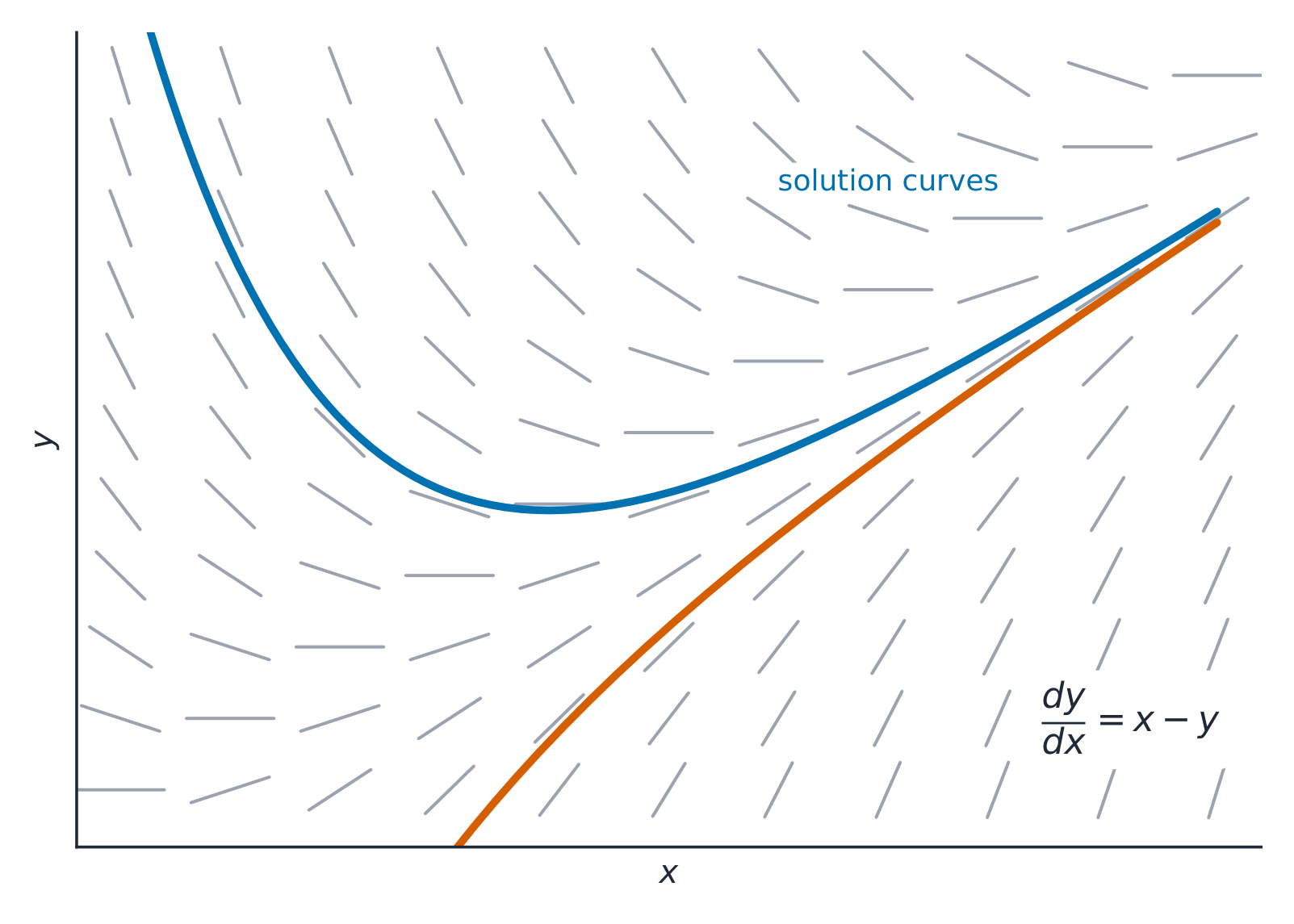
A slope field 斜率场 draws a short line segment at many points, each with the slope $\dfrac{dy}{dx}$ the equation gives there. It pictures the family of solution curves without solving. To sketch one, evaluate the right-hand side at each grid point and draw a segment of that slope.

Worked example. For $\dfrac{dy}{dx}=x-y$, substitute each point into $x-y$:

point $(x,y)$	$(0,0)$	$(1,0)$	$(0,1)$	$(1,1)$	$(2,1)$	$(-1,1)$
slope $x-y$	$0$	$1$	$-1$	$0$	$1$	$-2$

Every point on the line $y=x$ has slope $0$ (flat segments), and every point on $y=x-1$ has slope $1$.

A solution curve 解曲线 follows the segments like a boat following a current. From a slope field you can sketch the particular solution through a given point, describe long-run behavior, and locate where solutions level off (slopes near zero) – reasoning about solutions purely from the picture.

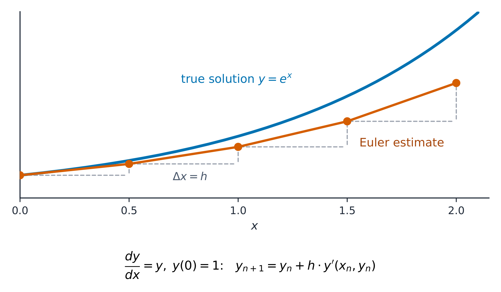
Euler's method 欧拉方法 approximates a solution numerically by stepping along the slope field. Starting from a known point, take a small step $\Delta x$ and update:

Repeat for each step. Smaller steps give a better approximation 近似值. (This is a BC-only technique.)

Exam skill: be able to carry out two or three Euler steps by hand from a table, and know that Euler's method underestimates 低估 or overestimates 高估 depending on the solution's concavity.

Worked example. Approximate $y(1)$ for $\dfrac{dy}{dx}=x+y$, $y(0)=1$, with step $\Delta x=0.5$. Step 1: slope at $(0,1)$ is $0+1=1$, so $y(0.5)\approx 1+1(0.5)=1.5$. Step 2: slope at $(0.5,1.5)$ is $0.5+1.5=2$, so $y(1)\approx 1.5+2(0.5)=2.5$.

Common mistakes. Forgetting to multiply the slope by $\Delta x$, and working out each slope from the original point instead of the point you have just reached: step 2 uses $(0.5,\,1.5)$.

Over or under? Differentiate the equation: $\dfrac{d^2y}{dx^2}=1+\dfrac{dy}{dx}=1+x+y$, which is positive near these points. The solution is concave up, so each tangent step lies below the curve and $2.5$ is an underestimate. (The exact solution is $y=2e^x-x-1$, so $y(1)=2e-2\approx 3.44$.)

In separation of variables 分离变量法, a separable 可分离 differential equation is written with all the $y$'s on one side and all the $x$'s on the other, then integrated (where the divided factor is nonzero):

This produces the general solution (with a $+C$), the main analytic method for solving differential equations in this course. Also check constant solutions 常数解 with $h(y)=0$ separately; division by $h(y)$ can lose them.

Worked example. Solve $\dfrac{dy}{dx}=xy$ with $y(0)=2$. Separating, $\int\frac{dy}{y}=\int x\,dx$ gives $\ln|y|=\frac{x^2}{2}+C$, so $y=Ae^{x^2/2}$. The condition $y(0)=2$ gives $A=2$, so $y=2e^{x^2/2}$.

Common mistakes. Adding the constant at the end: $y=e^{x^2/2}+C$ is wrong, because the constant enters when you integrate and becomes the multiplier $A=e^{C}$. Trying to separate an equation such as $\dfrac{dy}{dx}=x+y$: a sum cannot be written as $g(x)\,h(y)$.

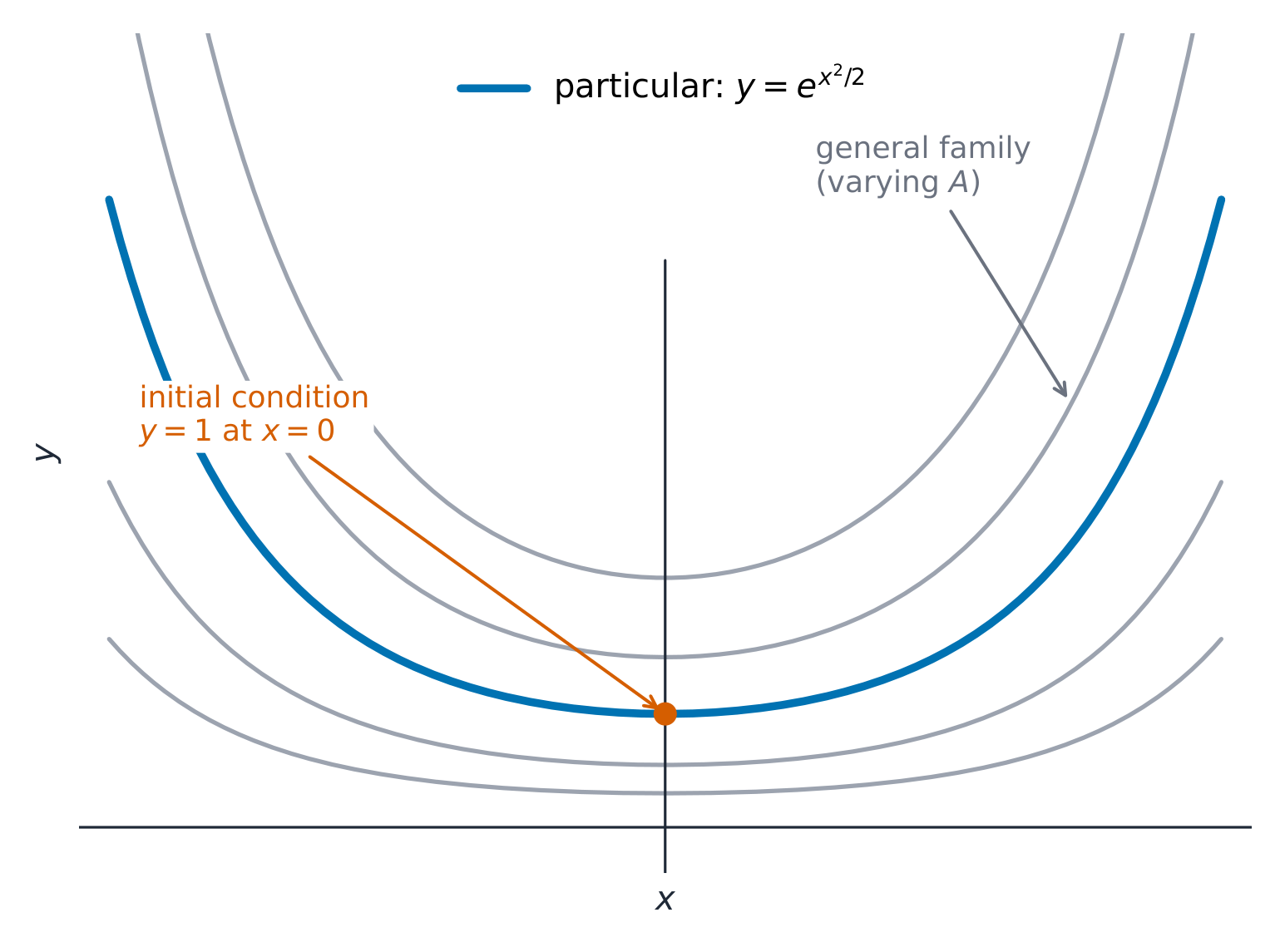
An initial condition 初始条件 (a known point, e.g. $y(0)=5$) pins down the constant $C$. Solve for the general solution, substitute the condition to find $C$, then write the particular solution. Watch the domain 定义域 – a particular solution is valid only on the interval containing the initial point.

Worked example. Solve $\dfrac{dy}{dx}=\dfrac{x}{y}$ with $y(0)=-3$. Separating gives $\dfrac{y^2}{2}=\dfrac{x^2}{2}+C$. Substitute the initial point now: $\tfrac92=C$, so $y^2=x^2+9$. The initial value is negative, so take the negative root:

The positive root fails $y(0)=-3$; choosing the sign from the initial condition is a scored step.

The equation $\dfrac{dy}{dt}=ky$ says the rate of change is proportional to the amount – giving exponential growth or decay 指数增长或衰减. Separating variables yields

with $k>0$ for growth and $k<0$ for decay. This models unrestricted population growth, radioactive decay 放射性衰变, and continuously compounded interest 连续复利.

Worked example: Newton's law of cooling. Coffee at $90^{\circ}$C cools in a room at $20^{\circ}$C by $\dfrac{dT}{dt}=-k\,(T-20)$, with $t$ in minutes. After $5$ minutes it is $70^{\circ}$C. When does it reach $40^{\circ}$C?

The difference $T-20$ decays exponentially from $90-20=70$, so

From $T(5)=70$: $50=70e^{-5k}$, so $k=\dfrac{\ln(7/5)}{5}\approx 0.0673$. For $T=40$: $20=70e^{-kt}$, so $t=\dfrac{\ln 3.5}{k}\approx 18.6$ minutes. Writing $T=90e^{-kt}$ (cooling towards $0^{\circ}$C) is the common error.

Real growth is limited by resources, so the logistic model 逻辑斯蒂模型 adds a carrying capacity 环境容纳量 $L$:

For $k>0$, $L>0$ and $0<P(0)<L$, growth is nearly exponential when $P$ is small, then the growth rate falls after $P=L/2$ as the population approaches $L$. The states $P=0$ and $P=L$ are equilibrium solutions 平衡解; a population initially at zero stays zero. Key BC facts: the population levels off at $L$ ($\lim_{t\to\infty}P=L$), and it grows fastest when $P=\tfrac{L}{2}$ (the inflection point of the S-shaped curve). You are expected to read $L$ and the fastest-growth value directly from the equation. If $P(0)>L$, the population instead decreases towards $L$, so $\lim_{t\to\infty}P=L$ still holds.

Worked example. For $\dfrac{dP}{dt}=0.05\,P\!\left(1-\dfrac{P}{2000}\right)$, the carrying capacity is $L=2000$ (the population levels off there), and growth is fastest when $P=\dfrac{L}{2}=1000$ – both read straight off the equation, no solving needed.

Common mistakes. Saying growth is fastest when $P=L$: at $P=L$ the growth rate is $0$. Giving a time when the question asks for the population at which growth is fastest ($P=1000$).

• Solve a separable equation by getting all $y$ on one side and all $x$ on the other, then integrating both sides (add $+C$ once).
• Use the initial condition to find $C$ (a particular solution).
• Sketch or read a slope field: the little segments show $\tfrac{dy}{dx}$ at each point, and a solution curve follows them.
• Recognise exponential models $\tfrac{dy}{dt}=ky\Rightarrow y=Ce^{kt}$ (growth/decay).
• A differential equation gives the slope — you must integrate to recover the function.