AP Statistics bao gồm khám phá dữ liệu, lấy mẫu và thiết kế thực nghiệm, xác suất và biến ngẫu nhiên, phân phối lấy mẫu và suy luận — khoảng tin cậy và kiểm định ý nghĩa. Có rất ít đại số; độ khó nằm ở việc nói đúng về sự không chắc chắn.
Mọi câu trả lời suy luận đều có bốn phần: đặt tên quy trình, kiểm tra điều kiện, tính toán và kết luận trong ngữ cảnh với liên kết đến giả thuyết thay thế. Bảng chấm điểm đánh giá cả bốn phần, nên chỉ có p-value chính xác thì điểm số vẫn thấp.
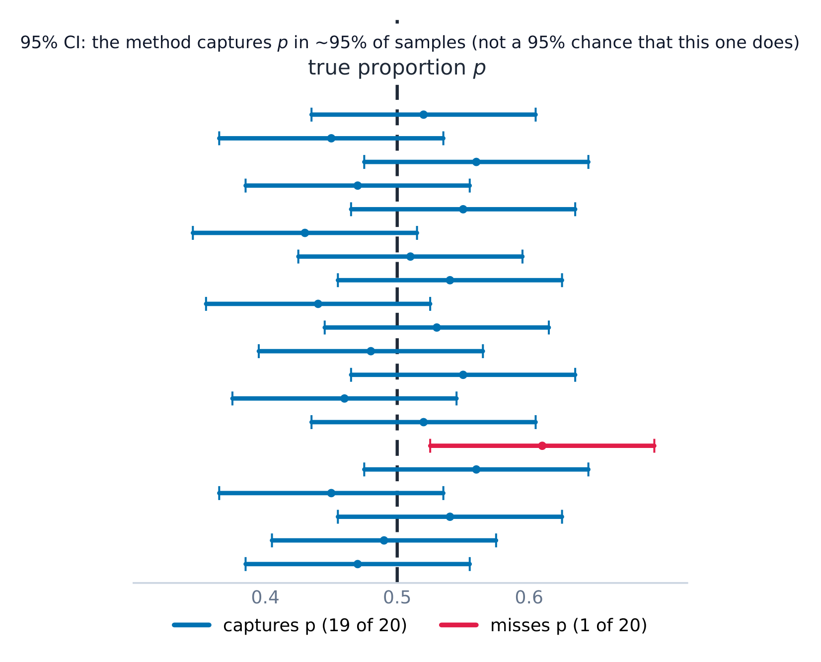
Ngôn ngữ được chấm điểm. "Chúng tôi bác bỏ H₀" không phải là "chúng tôi chứng minh H₁"; khoảng tin cậy nói về hành vi dài hạn của phương pháp, chứ không phải xác suất một khoảng cụ thể chứa tham số. Những phân biệt này quyết định điểm số.
Các ghi chú đi qua tất cả chín đơn vị với mỗi quy trình suy luận được trình bày từng bước. Các FRQs đã công bố có trong thư viện. Thống kê cho điểm khi nêu rõ điều kiện và diễn giải trong ngữ cảnh, vì vậy mọi câu trả lời hướng dẫn đều nêu các điều kiện trước khi tiến hành kiểm định.
Introducing Statistics: What Can We Learn from Data?
Syllabus · Chương trình
English
Enduring Understanding (VAR-1): Given that variation may be random or not, conclusions are uncertain.
Learning Objective VAR-1.A: Identify questions to be answered, based on variation in one-variable data. [Skill 1.A]
VAR-1.A.1 Numbers may convey meaningful information, when placed in context.
Tiếng Việt
Hiểu biết bền vững (VAR-1): Vì sự biến thiên có thể ngẫu nhiên hoặc không, nên những kết luận đều mang tính bất định.
Mục tiêu học tập VAR-1.A: Xác định các câu hỏi cần trả lời, dựa trên sự biến thiên của dữ liệu một biến. [Kỹ năng 1.A]
VAR-1.A.1 Các con số có thể truyền tải thông tin có ý nghĩa, khi được đặt trong ngữ cảnh.
Source: College Board AP Course and Exam Description · Nguồn: Mô tả Khóa học và Bài thi College Board AP
Statistics 统计学 is the science of learning from data 数据 – numbers or labels collected from the real world. Data vary, so we describe patterns and account for the variation 变异 rather than expecting every value to match. A statistical question anticipates an answer based on data that vary.
Two distinctions run through the whole course. A parameter 参数 is a numerical summary of a whole population; a statistic 统计量 is a numerical summary of a sample - we use the statistic to estimate the parameter we cannot measure directly. And descriptive statistics 描述统计 only summarise the data set in hand, while inferential statistics 推断统计 use a sample to make and test claims about the larger population.
Enduring Understanding (VAR-1): Given that variation may be random or not, conclusions are uncertain.
Learning Objective VAR-1.B: Identify variables in a set of data. [Skill 2.A]
VAR-1.B.1 A variable is a characteristic that changes from one individual to another.
Learning Objective VAR-1.C: Classify types of variables. [Skill 2.A]
VAR-1.C.1 A categorical variable takes on values that are category names or group labels.
VAR-1.C.2 A quantitative variable is one that takes on numerical values for a measured or counted quantity.
Illustrative examples for VAR-1.C:
Categorical variables:
Dominant hand
Age group (young or old)
Highest degree earned
Quantitative variables:
Age of a structure
Height of a child
Concentration of a sample
Tiếng Việt
Hiểu biết bền vững (VAR-1): Vì sự biến thiên có thể ngẫu nhiên hoặc không, nên những kết luận đều mang tính bất định.
Mục tiêu học tập VAR-1.B: Xác định các biến số trong một bộ dữ liệu. [Kỹ năng 2.A]
VAR-1.B.1 Một biến số là một đặc điểm thay đổi từ cá thể này sang cá thể khác.
Mục tiêu học tập VAR-1.C: Phân loại các loại biến số. [Kỹ năng 2.A]
VAR-1.C.1 Một biến số phân loại nhận các giá trị là tên phân loại hoặc nhãn nhóm.
VAR-1.C.2 Một biến số định lượng là biến số nhận các giá trị số học cho một đại lượng được đo lường hoặc đếm được.
Ví dụ minh họa cho VAR-1.C:
Biến số phân loại:
Tay chủ yếu
Nhóm tuổi (trẻ hoặc già)
Trình độ học vấn cao nhất đạt được
Các biến định lượng:
Tuổi của một công trình
Chiều cao của một đứa trẻ
Nồng độ của một mẫu thử
Source: College Board AP Course and Exam Description · Nguồn: Mô tả Khóa học và Bài thi College Board AP
A variable 变量 is a characteristic that can differ between individuals. Two kinds:
Categorical 分类 (qualitative): values are labels/groups (eye colour, brand).
Quantitative 定量: values are numbers you can do arithmetic on (height, age). Quantitative variables are discrete (countable) or continuous (measured).
Choosing the right graph and summary depends on which kind you have.
Explore · Khám phá
Categorical or quantitative? · Định tính hay Định lượng?
Every variable is either categorical (it labels each unit with a group) or quantitative (a measured number you can average). Which kind it is decides the graphs and summaries you are allowed to use. · Mọi biến đều là phân loại (nó gán đơn vị vào một nhóm) hoặc định lượng (một con số đo lường bạn có thể lấy trung bình). Loại nào quyết định biểu đồ và tóm tắt bạn được phép sử dụng.
Enduring Understanding (UNC-1): Graphical representations and statistics allow us to identify and represent key features of data.
Learning Objective UNC-1.A: Represent categorical data using frequency or relative frequency tables. [Skill 2.B]
UNC-1.A.1 A frequency table gives the number of cases falling into each category. A relative frequency table gives the proportion of cases falling into each category.
Learning Objective UNC-1.B: Describe categorical data represented in frequency or relative tables. [Skill 2.A]
UNC-1.B.1 Percentages, relative frequencies, and rates all provide the same information as proportions.
UNC-1.B.2 Counts and relative frequencies of categorical data reveal information that can be used to justify claims about the data in context.
Tiếng Việt
Hiểu biết bền vững (UNC-1): Các biểu đồ và số liệu thống kê giúp chúng ta xác định và biểu diễn các đặc điểm chính của dữ liệu.
Mục tiêu học tập UNC-1.A: Biểu diễn dữ liệu định tính bằng bảng tần số hoặc tần số tương đối. [Kỹ năng 2.B]
UNC-1.A.1 Bảng tần số cho biết số trường hợp落入 vào mỗi danh mục. Bảng tần số tương đối cho biết tỷ lệ phần trăm các trường hợp落入 vào mỗi danh mục.
Mục tiêu học tập UNC-1.B: Mô tả dữ liệu định tính được biểu diễn trong bảng tần số hoặc bảng tần số tương đối. [Kỹ năng 2.A]
UNC-1.B.1 Phần trăm, tần số tương đối và tốc độ đều cung cấp cùng thông tin với tỷ lệ phần trăm.
UNC-1.B.2 Số lượng và tần số tương đối của dữ liệu định tính tiết lộ thông tin có thể được sử dụng để biện minh cho các tuyên bố về dữ liệu trong ngữ cảnh.
Source: College Board AP Course and Exam Description · Nguồn: Mô tả Khóa học và Bài thi College Board AP
A frequency table 频数表 lists each category's count (frequency); a relative frequency 相对频率 table lists each category's proportion 比例 (count ÷ total). Relative frequencies let you compare groups of different sizes fairly.
UNC-1.E.1 Frequency tables, bar graphs, or other representations can be used to compare two or more data sets in terms of the same categorical variable.
Tiếng Việt
Hiểu biết bền vững (UNC-1): Các biểu đồ và số liệu thống kê giúp chúng ta xác định và biểu diễn các đặc điểm chính của dữ liệu.
Mục tiêu học tập UNC-1.C: Biểu diễn dữ liệu định tính bằng đồ thị. [Kỹ năng 2.B]
UNC-1.C.1 Biểu đồ cột (hoặc biểu đồ thanh) được sử dụng để hiển thị tần số (số lượng) hoặc tần số tương đối (tỷ lệ phần trăm) cho dữ liệu định tính.
UNC-1.C.2 Chiều cao hoặc chiều dài của mỗi cột trong biểu đồ cột tương ứng với số lượng hoặc tỷ lệ phần trăm các quan sát落入 trong mỗi danh mục.
UNC-1.C.3 Có rất nhiều cách khác để biểu diễn tần số (số lượng) hoặc tần số tương đối (tỷ lệ phần trăm) cho dữ liệu định tính.
Mục tiêu học tập UNC-1.D: Mô tả dữ liệu định tính được biểu diễn bằng đồ thị. [Kỹ năng 2.A]
UNC-1.D.1 Các biểu diễn đồ thị của biến định tính tiết lộ thông tin có thể được sử dụng để biện minh cho các tuyên bố về dữ liệu trong ngữ cảnh.
Mục tiêu học tập UNC-1.E: So sánh nhiều bộ dữ liệu định tính. [Kỹ năng 2.D]
UNC-1.E.1 Bảng tần số, biểu đồ cột hoặc các biểu diễn khác có thể được sử dụng để so sánh hai hoặc nhiều bộ dữ liệu theo cùng một biến định tính.
Source: College Board AP Course and Exam Description · Nguồn: Mô tả Khóa học và Bài thi College Board AP
Bar charts 条形图 show the count or proportion of each category as separated bars; a pie chart shows each category's share of the whole. The bar heights (or slices) let you compare categories at a glance. Bars may be ordered by size or by a natural category order.
Explore · Khám phá
Show a categorical variable as a pie chart · Hiển thị biến phân loại dưới dạng biểu đồ tròn
A pie chart turns each category's share of the whole into a slice: a bigger share is a bigger slice, and every slice together makes 100%. It is a picture of a relative-frequency table. · Một biểu đồ tròn biến tỷ lệ phần trăm của mỗi danh mục so với tổng thể thành một miếng: tỷ lệ lớn hơn thì miếng lớn hơn, và tất cả các miếng cộng lại tạo thành 100%. Nó là hình ảnh của bảng tần suất tương đối.
Enduring Understanding (UNC-1): Graphical representations and statistics allow us to identify and represent key features of data.
Learning Objective UNC-1.F: Classify types of quantitative variables. [Skill 2.A]
UNC-1.F.1 A discrete variable can take on a countable number of values. The number of values may be finite or countably infinite, as with the counting numbers.
UNC-1.F.2 A continuous variable can take on infinitely many values, but those values cannot be counted. No matter how small the interval between two values of a continuous variable, it is always possible to determine another value between them.
Illustrative examples for UNC-1.F:
A discrete variable:
Number of students in a class
A continuous variable:
Height of a child
Learning Objective UNC-1.G: Represent quantitative data graphically. [Skill 2.B]
UNC-1.G.1 In a histogram, the height of each bar shows the number or proportion of observations that fall within the interval corresponding to that bar. Altering the interval widths can change the appearance of the histogram.
UNC-1.G.2 In a stem and leaf plot, each data value is split into a "stem" (the first digit or digits) and a "leaf" (usually the last digit).
UNC-1.G.3 A dotplot represents each observation by a dot, with the position on the horizontal axis corresponding to the data value of that observation, with nearly identical values stacked on top of each other.
UNC-1.G.4 A cumulative graph represents the number or proportion of a data set less than or equal to a given number.
UNC-1.G.5 There are many additional ways to graphically represent distributions of quantitative data.
Tiếng Việt
Hiểu biết bền vững (UNC-1): Các biểu đồ và số liệu thống kê giúp chúng ta xác định và biểu diễn các đặc điểm chính của dữ liệu.
Mục tiêu học tập UNC-1.F: Phân loại các loại biến định lượng. [Kỹ năng 2.A]
UNC-1.F.1 Biến rời rạc có thể nhận một số giá trị đếm được. Số giá trị có thể hữu hạn hoặc vô hạn đếm được, ví dụ như các số đếm.
UNC-1.F.2 Biến liên tục có thể nhận vô số giá trị, nhưng những giá trị đó không thể đếm được. Bất kể khoảng cách giữa hai giá trị của biến liên tục nhỏ đến đâu, luôn có thể xác định được một giá trị khác nằm giữa chúng.
Ví dụ minh họa cho UNC-1.F:
Một biến rời rạc:
Số học sinh trong một lớp
Một biến liên tục:
Chiều cao của một đứa trẻ
Mục tiêu học tập UNC-1.G: Biểu diễn dữ liệu định lượng bằng đồ thị. [Kỹ năng 2.B]
UNC-1.G.1 Trong biểu đồ tần số (histogram), chiều cao của mỗi cột cho biết số lượng hoặc tỷ lệ phần trăm các quan sát落入 trong khoảng tương ứng với cột đó. Thay đổi độ rộng khoảng có thể làm thay đổi hình dáng của biểu đồ tần số.
UNC-1.G.2 Trong biểu đồ thân lá, mỗi giá trị dữ liệu được chia thành "thân" (chữ số đầu tiên hoặc các chữ số đầu) và "lá" (thường là chữ số cuối).
UNC-1.G.3 Biểu đồ chấm biểu diễn mỗi quan sát bằng một chấm, với vị trí trên trục hoành tương ứng với giá trị dữ liệu của quan sát đó, với các giá trị gần giống nhau xếp chồng lên nhau.
UNC-1.G.4 Biểu đồ tích lũy biểu diễn số lượng hoặc tỷ lệ phần trăm của bộ dữ liệu nhỏ hơn hoặc bằng một số đã cho.
UNC-1.G.5 Có rất nhiều cách khác để biểu diễn đồ thị phân phối của dữ liệu định lượng.
Source: College Board AP Course and Exam Description · Nguồn: Mô tả Khóa học và Bài thi College Board AP
For numbers, use a dotplot 点图, stem-and-leaf plot 茎叶图, or histogram 直方图 (bars over value intervals called bins). These show the distribution 分布 – how the values spread out. A histogram's bin width changes the picture, so choose it to reveal the shape.
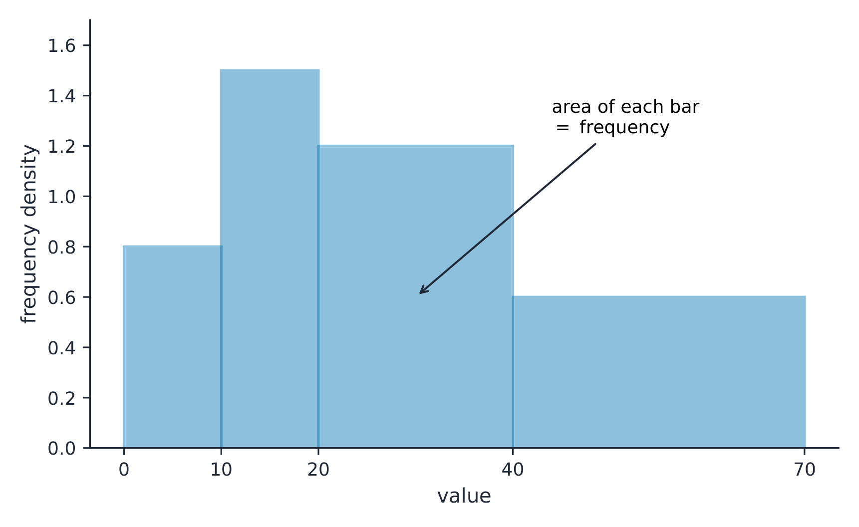
On a histogram with unequal class widths the bar area is the frequency
Explore · Khám phá
Explore how bin width shapes a histogram · Khám phá cách độ rộng ô ảnh hưởng đến biểu đồ tần suất
A histogram groups data into equal-width bins and draws a bar over each. Change the bins and notice how the same data can look jagged (too narrow) or smooth (too wide) — the shape is a choice. · Một biểu đồ tần suất nhóm dữ liệu thành các ô có chiều rộng bằng nhau và vẽ một thanh trên mỗi ô. Thay đổi các ô và để ý rằng cùng một dữ liệu có thể trông gợn sóng (quá hẹp) hoặc mịn màng (quá rộng) — hình dạng là một sự lựa chọn.
Describing the Distribution of a Quantitative Variable
Syllabus · Chương trình
English
Enduring Understanding (UNC-1): Graphical representations and statistics allow us to identify and represent key features of data.
Learning Objective UNC-1.H: Describe the characteristics of quantitative data distributions. [Skill 2.A]
UNC-1.H.1 Descriptions of the distribution of quantitative data include shape, center, and variability (spread), as well as any unusual features such as outliers, gaps, clusters, or multiple peaks.
UNC-1.H.2 Outliers for one-variable data are data points that are unusually small or large relative to the rest of the data.
UNC-1.H.3 A distribution is skewed to the right (positive skew) if the right tail is longer than the left. A distribution is skewed to the left (negative skew) if the left tail is longer than the right. A distribution is symmetric if the left half is the mirror image of the right half.
UNC-1.H.4 Univariate graphs with one main peak are known as unimodal. Graphs with two prominent peaks are bimodal. A graph where each bar height is approximately the same (no prominent peaks) is approximately uniform.
UNC-1.H.5 A gap is a region of a distribution between two data values where there are no observed data.
UNC-1.H.6 Clusters are concentrations of data usually separated by gaps.
UNC-1.H.7 Descriptive statistics does not attribute properties of a data set to a larger population, but may provide the basis for conjectures for subsequent testing.
Tiếng Việt
Hiểu biết bền vững (UNC-1): Các biểu đồ và số liệu thống kê giúp chúng ta xác định và biểu diễn các đặc điểm chính của dữ liệu.
Mục tiêu học tập UNC-1.H: Mô tả các đặc điểm của phân phối dữ liệu định lượng. [Kỹ năng 2.A]
UNC-1.H.1 Mô tả phân phối của dữ liệu định lượng bao gồm hình dạng, trung tâm và độ biến thiên (phân tán), cũng như bất kỳ đặc điểm bất thường nào như giá trị ngoại lai, khoảng trống, cụm dữ liệu, hoặc nhiều đỉnh.
UNC-1.H.2 Giá trị ngoại lai cho dữ liệu một biến là các điểm dữ liệu bất thường nhỏ hoặc lớn so với phần còn lại của dữ liệu.
UNC-1.H.3 Phân phối lệch về bên phải (lệch dương) nếu đuôi bên phải dài hơn đuôi bên trái. Phân phối lệch về bên trái (lệch âm) nếu đuôi bên trái dài hơn đuôi bên phải. Phân phối đối xứng nếu nửa bên trái là ảnh phản chiếu của nửa bên phải.
UNC-1.H.4 Đồ thị một biến với một đỉnh chính được gọi là đơn modal. Đồ thị với hai đỉnh nổi bật là song modal. Đồ thị mà chiều cao của mỗi cột xấp xỉ bằng nhau (không có đỉnh nổi bật) là xấp xỉ đồng đều.
UNC-1.H.5 Khoảng trống là một vùng của phân phối giữa hai giá trị dữ liệu nơi không có dữ liệu quan sát nào.
UNC-1.H.6 Cụm dữ liệu là sự tập trung của dữ liệu thường được tách biệt bởi các khoảng trống.
UNC-1.H.7 Thống kê mô tả không gán các thuộc tính của bộ dữ liệu cho quần thể lớn hơn, nhưng có thể cung cấp cơ sở cho các phỏng đoán để kiểm tra tiếp theo.
Source: College Board AP Course and Exam Description · Nguồn: Mô tả Khóa học và Bài thi College Board AP
Describe four things (remember SOCS):
Shape 形状: symmetric, or skewed 偏斜 left/right (a long tail on that side), and how many peaks - one main peak is unimodal 单峰, two prominent peaks bimodal 双峰, and roughly equal bars uniform 均匀.
Outliers 离群值: unusual values far from the rest.
Center: a typical value (mean or median).
Spread: how much the values vary (range, IQR, standard deviation).
Always describe shape/center/spread in context, with units.
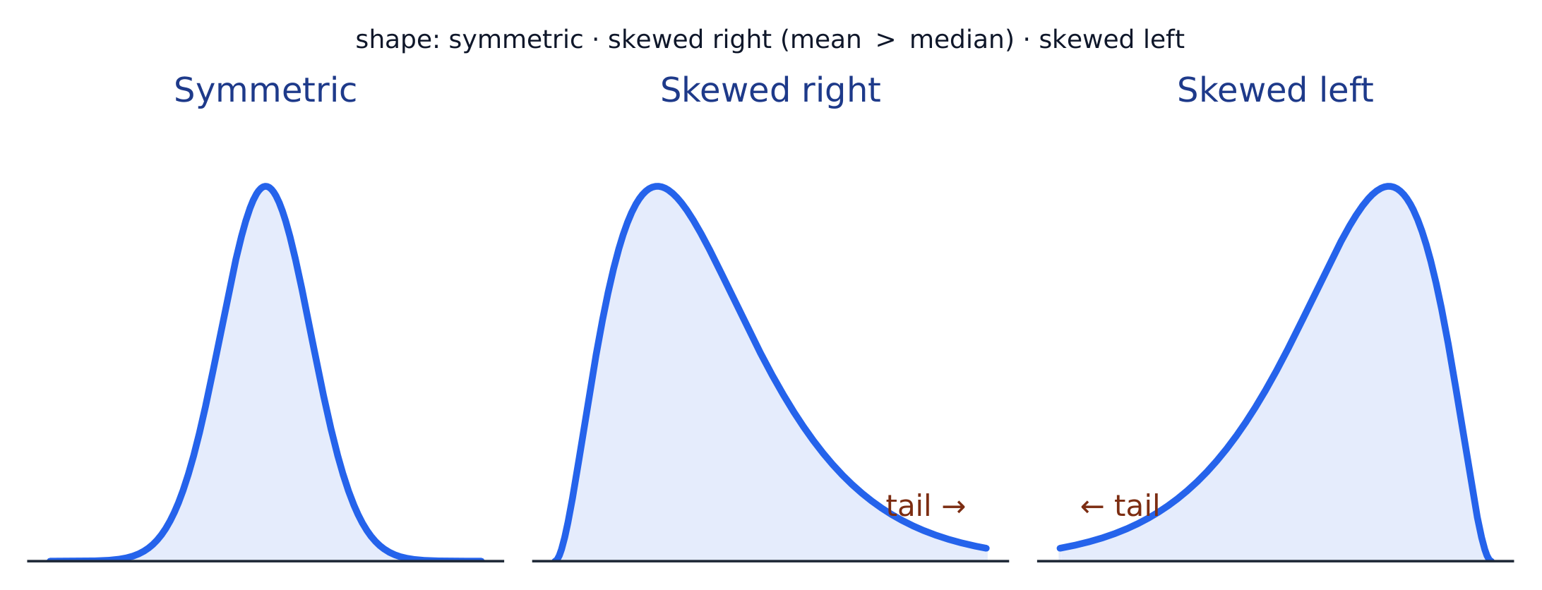
The shape of a distribution: symmetric, skewed right (long right tail), or skewed left
Enduring Understanding (UNC-1): Graphical representations and statistics allow us to identify and represent key features of data.
Learning Objective UNC-1.I: Calculate measures of center and position for quantitative data. [Skill 2.C]
UNC-1.I.1 A statistic is a numerical summary of sample data.
UNC-1.I.2 The mean is the sum of all the data values divided by the number of values. For a sample, the mean is denoted by $x$-bar: $\bar{x} = \dfrac{1}{n}\sum_{i=1}^{n} x_i$, where $x_i$ represents the $i^{\text{th}}$ data point in the sample and $n$ represents the number of data values in the sample.
UNC-1.I.3 The median of a data set is the middle value when data are ordered. When the number of data points is even, the median can take on any value between the two middle values. In AP Statistics, the most commonly used value for the median of a data set with an even number of values is the average of the two middle values.
UNC-1.I.4 The first quartile, Q1, is the median of the half of the ordered data set from the minimum to the position of the median. The third quartile, Q3, is the median of the half of the ordered data set from the position of the median to the maximum. Q1 and Q3 form the boundaries for the middle 50% of values in an ordered data set.
UNC-1.I.5 The $p^{\text{th}}$ percentile is interpreted as the value that has $p\%$ of the data less than or equal to it.
Learning Objective UNC-1.J: Calculate measures of variability for quantitative data. [Skill 2.C]
UNC-1.J.1 Three commonly used measures of variability (or spread) in a distribution are the range, interquartile range, and standard deviation.
UNC-1.J.2 The range is defined as the difference between the maximum data value and the minimum data value. The interquartile range (IQR) is defined as the difference between the third and first quartiles: $Q3 - Q1$. Both the range and the interquartile range are possible ways of measuring variability of the distribution of a quantitative variable.
UNC-1.J.3 Standard deviation is a way to measure variability of the distribution of a quantitative variable. For a sample, the standard deviation is denoted by $s$: $s_x = \sqrt{\dfrac{1}{n-1}\sum(x_i - \bar{x})^2}$. The square of the sample standard deviation, $s^2$, is called the sample variance.
UNC-1.J.4 Changing units of measurement affects the values of the calculated statistics.
Learning Objective UNC-1.K: Explain the selection of a particular measure of center and/or variability for describing a set of quantitative data. [Skill 4.B]
UNC-1.K.1 There are many methods for determining outliers. Two methods frequently used in this course are:
UNC-1.K.1.i An outlier is a value greater than $1.5 \times \text{IQR}$ above the third quartile or more than $1.5 \times \text{IQR}$ below the first quartile.
UNC-1.K.1.ii An outlier is a value located 2 or more standard deviations above, or below, the mean.
UNC-1.K.2 The mean, standard deviation, and range are considered nonresistant (or non-robust) because they are influenced by outliers. The median and IQR are considered resistant (or robust), because outliers do not greatly (if at all) affect their value.
Tiếng Việt
Hiểu biết bền vững (UNC-1): Các biểu đồ và số liệu thống kê giúp chúng ta xác định và biểu diễn các đặc điểm chính của dữ liệu.
Mục tiêu học tập UNC-1.I: Tính toán các thước đo trung tâm và vị trí cho dữ liệu định lượng. [Kỹ năng 2.C]
UNC-1.I.1 Một số liệu thống kê là một bản tóm tắt số học của dữ liệu mẫu.
UNC-1.I.2 Trung bình cộng là tổng của tất cả các giá trị dữ liệu chia cho số lượng giá trị. Đối với mẫu, trung bình cộng được ký hiệu là $x$-bar: $\bar{x} = \dfrac{1}{n}\sum_{i=1}^{n} x_i$, trong đó $x_i$ đại diện cho $i^{\text{th}}$ điểm dữ liệu trong mẫu và $n$ đại diện cho số lượng giá trị dữ liệu trong mẫu.
UNC-1.I.3 Median (trung vị) của một tập dữ liệu là giá trị ở giữa khi dữ liệu đã được sắp xếp. Khi số lượng điểm dữ liệu là số chẵn, median có thể nhận bất kỳ giá trị nào nằm giữa hai giá trị ở giữa. Trong AP Statistics, giá trị thường dùng nhất cho median của tập dữ liệu có số lượng giá trị chẵn là trung bình cộng của hai giá trị ở giữa.
UNC-1.I.4 Tứ phân vị thứ nhất, Q1, là median của nửa tập dữ liệu đã sắp xếp từ giá trị tối thiểu đến vị trí của median. Tứ phân vị thứ ba, Q3, là median của nửa tập dữ liệu đã sắp xếp từ vị trí của median đến giá trị tối đa. Q1 và Q3 tạo thành ranh giới cho 50% giá trị ở giữa trong một tập dữ liệu đã sắp xếp.
UNC-1.I.5 P $p^{\text{th}}$ phần trăm được hiểu là giá trị mà $p\%$ của dữ liệu nhỏ hơn hoặc bằng nó.
Mục tiêu học tập UNC-1.J: Tính toán các Measures of variability (đo lường độ phân tán) cho dữ liệu định lượng. [Kỹ năng 2.C]
UNC-1.J.1 Ba Measures of variability (hoặc spread - độ trải rộng) thường dùng trong phân phối là khoảng biến thiên (range), khoảng tứ phân vị (interquartile range), và độ lệch chuẩn.
UNC-1.J.2 Khoảng biến thiên (range) được định nghĩa là hiệu giữa giá trị dữ liệu lớn nhất và giá trị dữ liệu nhỏ nhất. Khoảng tứ phân vị (IQR) được định nghĩa là hiệu giữa tứ phân vị thứ ba và tứ phân vị thứ nhất: $Q3 - Q1$. Cả khoảng biến thiên và khoảng tứ phân vị đều là những cách đo lường độ phân tán hợp lý của phân phối một biến định lượng.
UNC-1.J.3 Độ lệch chuẩn là một cách để đo lường độ phân tán của phân phối một biến định lượng. Đối với mẫu, độ lệch chuẩn được ký hiệu là $s$: $s_x = \sqrt{\dfrac{1}{n-1}\sum(x_i - \bar{x})^2}$. Bình phương của độ lệch chuẩn mẫu, $s^2$, được gọi là phương sai mẫu.
UNC-1.J.4 Thay đổi đơn vị đo lường sẽ ảnh hưởng đến các giá trị thống kê đã tính toán.
Mục tiêu học tập UNC-1.K: Giải thích việc lựa chọn một Measure of center (đo lường trung tâm) và/hoặc Measure of variability (đo lường độ phân tán) cụ thể để mô tả một tập dữ liệu định lượng. [Kỹ năng 4.B]
UNC-1.K.1 Có nhiều phương pháp xác định giá trị ngoại lai. Hai phương pháp thường được sử dụng trong khóa học này là:
UNC-1.K.1.i Một giá trị ngoại lai là giá trị lớn hơn $1.5 \times \text{IQR}$ trên tứ phân vị thứ ba hoặc nhỏ hơn $1.5 \times \text{IQR}$ dưới tứ phân vị thứ nhất.
UNC-1.K.1.ii Một giá trị ngoại lai là giá trị nằm cách 2 hoặc nhiều độ lệch chuẩn hơn lên trên, hoặc xuống dưới, trung bình cộng.
UNC-1.K.2 Trung bình cộng, độ lệch chuẩn và khoảng biến thiên được coi là không kháng cự (nonresistant hoặc non-robust) vì chúng bị ảnh hưởng bởi các giá trị ngoại lai. Median và IQR được coi là kháng cự (resistant hoặc robust), vì các giá trị ngoại lai không làm thay đổi đáng kể (nếu có) giá trị của chúng.
Source: College Board AP Course and Exam Description · Nguồn: Mô tả Khóa học và Bài thi College Board AP
Standard deviation: spread about the mean
Center: the mean 均值$\bar{x}=\dfrac{\sum x_i}{n}$ (average) and the median 中位数 (middle value). The median resists outliers; the mean is pulled toward a skew.
Spread: the range, the interquartile range 四分位距$\text{IQR}=Q_3-Q_1$ (middle 50%), and the standard deviation 标准差$s_x=\sqrt{\dfrac{\sum(x_i-\bar{x})^2}{n-1}}$ (typical distance from the mean; its square is the variance 方差).
The five-number summary 五数概括: min, $Q_1$, median, $Q_3$, max.
Use resistant measures (median, IQR) for skewed data; mean and standard deviation for roughly symmetric data.
The percentile 百分位数 of a value is the percent of the data at or below it – so the median is the 50th percentile and $Q_1$ the 25th. A cumulative relative frequency graph 累积相对频率图 makes percentiles easy to read: for each value it plots the proportion of the data at or below it, rising from 0 to 1. Go up from a value to the curve and across to its percentile, or reverse the steps to find the value at a given percentile (the same reading works from a cumulative-frequency table).
Worked example. For the data $4, 8, 6, 10, 7$: the mean is $\bar{x}=\dfrac{4+8+6+10+7}{5}=\dfrac{35}{5}=7$. Sorting to $4,6,7,8,10$, the median is the middle value, $7$. The mean and median agree here because the data are roughly symmetric.
cumulative relative frequency graph/ˈkjuːmjʊlətɪv ˈrelətɪv ˈfriːkwənsi ɡræf/
biểu đồ tần số tương đối lũy kế
1.8
Graphical Representations of Summary Statistics
Syllabus · Chương trình
English
Enduring Understanding (UNC-1): Graphical representations and statistics allow us to identify and represent key features of data.
Learning Objective UNC-1.L: Represent summary statistics for quantitative data graphically. [Skill 2.B]
UNC-1.L.1 Taken together, the minimum data value, the first quartile (Q1), the median, the third quartile (Q3), and the maximum data value make up the five-number summary.
UNC-1.L.2 A boxplot is a graphical representation of the five-number summary (minimum, first quartile, median, third quartile, maximum). The box represents the middle 50% of data, with a line at the median and the ends of the box corresponding to the quartiles. Lines ("whiskers") extend from the quartiles to the most extreme point that is not an outlier, and outliers are indicated by their own symbol beyond this.
Learning Objective UNC-1.M: Describe summary statistics of quantitative data represented graphically. [Skill 2.A]
UNC-1.M.1 Summary statistics of quantitative data, or of sets of quantitative data, can be used to justify claims about the data in context.
UNC-1.M.2 If a distribution is relatively symmetric, then the mean and median are relatively close to one another. If a distribution is skewed right, then the mean is usually to the right of the median. If the distribution is skewed left, then the mean is usually to the left of the median.
Tiếng Việt
Hiểu biết bền vững (UNC-1): Các biểu đồ và số liệu thống kê giúp chúng ta xác định và biểu diễn các đặc điểm chính của dữ liệu.
Mục tiêu học tập UNC-1.L: Biểu diễn đồ thị các Thống kê Tóm tắt cho dữ liệu định lượng. [Kỹ năng 2.B]
UNC-1.L.1 Kết hợp lại, giá trị dữ liệu tối thiểu, tứ phân vị thứ nhất (Q1), median, tứ phân vị thứ ba (Q3), và giá trị dữ liệu tối đa tạo thành bộ năm số tóm tắt (five-number summary).
UNC-1.L.2 Một boxplot (biểu đồ hộp) là biểu diễn đồ thị của bộ năm số tóm tắt (tối thiểu, tứ phân vị thứ nhất, median, tứ phân vị thứ ba, tối đa). Phần hộp đại diện cho 50% dữ liệu ở giữa, với đường kẻ tại vị trí median và hai đầu hộp tương ứng với các tứ phân vị. Các đường thẳng ("mũi") kéo dài từ các tứ phân vị đến điểm cực đoan nhất không phải là giá trị ngoại lai, và các giá trị ngoại lai được chỉ báo bằng ký hiệu riêng biệt bên ngoài điểm này.
Mục tiêu học tập UNC-1.M: Mô tả các Thống kê Tóm tắt của dữ liệu định lượng được biểu diễn đồ thị. [Kỹ năng 2.A]
UNC-1.M.1 Các Thống kê Tóm tắt của dữ liệu định lượng, hoặc các tập dữ liệu định lượng, có thể được sử dụng để biện minh cho các tuyên bố về dữ liệu trong ngữ cảnh cụ thể.
UNC-1.M.2 Nếu một phân phối khá đối xứng, thì trung bình cộng và median sẽ tương đối gần nhau. Nếu một phân phối lệch phải, thì trung bình cộng thường nằm bên phải của median. Nếu phân phối lệch trái, thì trung bình cộng thường nằm bên trái của median.
Source: College Board AP Course and Exam Description · Nguồn: Mô tả Khóa học và Bài thi College Board AP
A boxplot 箱线图 draws the five-number summary: a box from $Q_1$ to $Q_3$ with the median inside, and whiskers to the most extreme non-outlier values. A point is an outlier if it lies more than $1.5\times\text{IQR}$ beyond a quartile – a rule you may be asked to apply. Boxplots are ideal for comparing several groups side by side.
Worked example. A dataset has $Q_1=20$ and $Q_3=32$, so $\text{IQR}=12$. The outlier fences are $Q_1-1.5(12)=2$ and $Q_3+1.5(12)=50$. Any value below $2$ or above $50$ is flagged as an outlier.
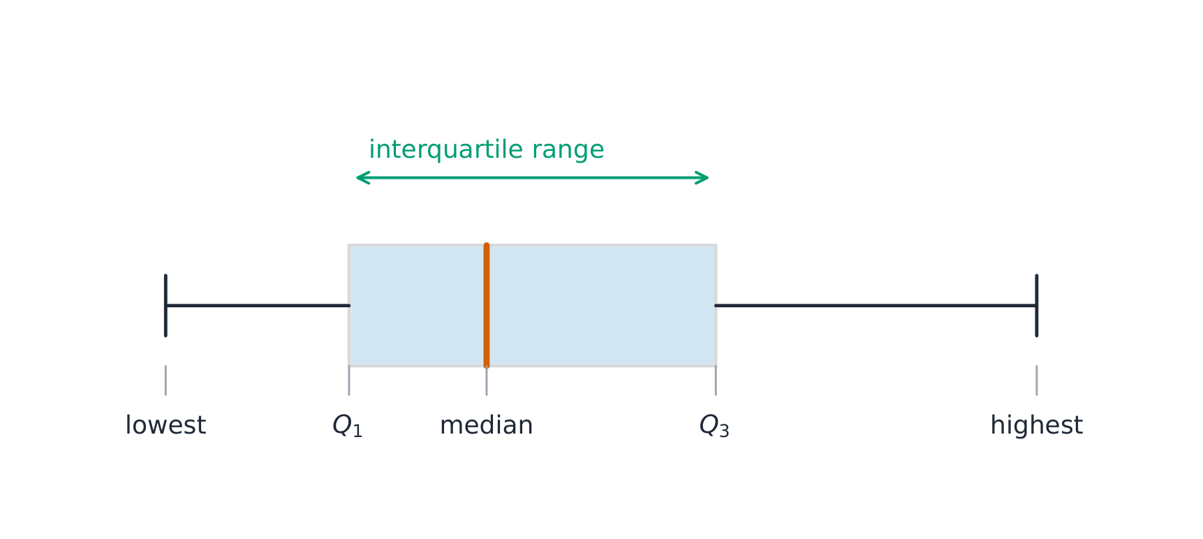
A box-and-whisker plot shows the quartiles and the rangeA boxplot draws the five-number summary; the box spans the IQR
Explore · Khám phá
Explore the five-number summary as a boxplot · Khám phá tóm tắt năm số dưới dạng hộp
Drag $Q_1$, the median, and $Q_3$ to see the box (its length is the IQR) and how the median's position inside the box reveals skew — a median close to $Q_1$ signals a right-skewed distribution. · Kéo $Q_1$, trung vị, và $Q_3$ để xem hộp (chiều dài của nó là IQR) và làm thế nào vị trí trung vị bên trong hộp tiết lộ độ lệch — trung vị gần $Q_1$ báo hiệu phân phối lệch phải.
Comparing Distributions of a Quantitative Variable
Syllabus · Chương trình
English
Enduring Understanding (UNC-1): Graphical representations and statistics allow us to identify and represent key features of data.
Learning Objective UNC-1.N: Compare graphical representations for multiple sets of quantitative data. [Skill 2.D]
UNC-1.N.1 Any of the graphical representations, e.g., histograms, side-by-side boxplots, etc., can be used to compare two or more independent samples on center, variability, clusters, gaps, outliers, and other features.
Learning Objective UNC-1.O: Compare summary statistics for multiple sets of quantitative data. [Skill 2.D]
UNC-1.O.1 Any of the numerical summaries (e.g., mean, standard deviation, relative frequency, etc.) can be used to compare two or more independent samples.
Tiếng Việt
Hiểu biết bền vững (UNC-1): Các biểu đồ và số liệu thống kê giúp chúng ta xác định và biểu diễn các đặc điểm chính của dữ liệu.
Mục tiêu học tập UNC-1.N: So sánh các biểu diễn đồ thị cho nhiều tập dữ liệu định lượng. [Kỹ năng 2.D]
UNC-1.N.1 Bất kỳ loại biểu diễn đồ thị nào, ví dụ: histogram, boxplot đặt cạnh nhau, v.v., đều có thể được sử dụng để so sánh hai hoặc nhiều mẫu độc lập về trung tâm, độ phân tán, cụm, khoảng trống, giá trị ngoại lai và các đặc điểm khác.
Mục tiêu học tập UNC-1.O: So sánh các Thống kê Tóm tắt cho nhiều tập dữ liệu định lượng. [Kỹ năng 2.D]
UNC-1.O.1 Bất kỳ loại tóm tắt số nào (ví dụ: trung bình cộng, độ lệch chuẩn, tần suất tương đối, v.v.) đều có thể được sử dụng để so sánh hai hoặc nhiều mẫu độc lập.
Source: College Board AP Course and Exam Description · Nguồn: Mô tả Khóa học và Bài thi College Board AP
To compare two or more groups, compare shape, center, and spread, and mention outliers – always with comparative words ("Group A has a higher median than Group B") and in context. Do not just describe each group separately; make the comparison explicit.
Explore · Khám phá
Compare distributions with box plots · So sánh phân phối với biểu đồ hộp
A box plot draws the five-number summary. Placing two box plots on the same scale compares their centre (median), spread (IQR = box width) and skew at a glance — the fair way to compare groups. · Một biểu đồ hộp vẽ tóm tắt năm số. Đặt hai biểu đồ hộp trên cùng một thang đo so sánh trung tâm (trung vị), độ phân tán (IQR = chiều rộng hộp) và độ lệch ngay lập tức — cách công bằng để so sánh các nhóm.
1.10
The Normal Distribution
Syllabus · Chương trình
Enduring Understanding
Learning Objective
Essential Knowledge
VAR-2
The normal distribution can be used to represent some population distributions.
VAR-2.A
Compare a data distribution to the normal distribution model. [Skill 2.D]
VAR-2.A.1 A parameter is a numerical summary of a population.
VAR-2.A.2 Some sets of data may be described as approximately normally distributed. A normal curve is mound-shaped and symmetric. The parameters of a normal distribution are the population mean, $\mu$, and the population standard deviation, $\sigma$.
VAR-2.A.3 For a normal distribution, approximately 68% of the observations are within 1 standard deviation of the mean, approximately 95% of observations are within 2 standard deviations of the mean, and approximately 99.7% of observations are within 3 standard deviations of the mean. This is called the empirical rule.
VAR-2.A.4 Many variables can be modeled by a normal distribution.
Illustrative examples for VAR-2.A:
Variables that can be modeled by a normal distribution:
Body temperature
Weight of a loaf of bread
VAR-2.B
Determine proportions and percentiles from a normal distribution. [Skill 3.A]
VAR-2.B.1 A standardized score for a particular data value is calculated as (data value − mean)/(standard deviation), and measures the number of standard deviations a data value falls above or below the mean.
VAR-2.B.2 One example of a standardized score is a $z$-score, which is calculated as $z\text{-score} = \left(\dfrac{x_i - \mu}{\sigma}\right)$. A $z$-score measures how many standard deviations a data value is from the mean.
VAR-2.B.3 Technology, such as a calculator, a standard normal table, or computer-generated output, can be used to find the proportion of data values located on a given interval of a normally distributed random variable.
VAR-2.B.4 Given the area of a region under the graph of the normal distribution curve, it is possible to use technology, such as a calculator, a standard normal table, or computer-generated output, to estimate parameters for some populations.
VAR-2.C
Compare measures of relative position in data sets. [Skill 2.D]
VAR-2.C.1 Percentiles and $z$-scores may be used to compare relative positions of points within a data set or between data sets.
Source: College Board AP Course and Exam Description · Nguồn: Mô tả Khóa học và Bài thi College Board AP
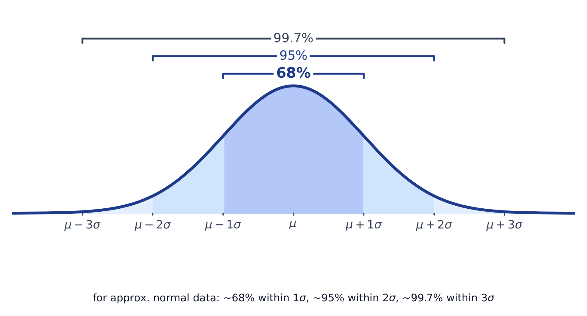
A normal distribution 正态分布 is a symmetric, bell-shaped model described by its mean $\mu$ and standard deviation $\sigma$. The empirical rule 经验法则 (68–95–99.7): about 68% of values lie within $1\sigma$ of the mean, 95% within $2\sigma$, and 99.7% within $3\sigma$.
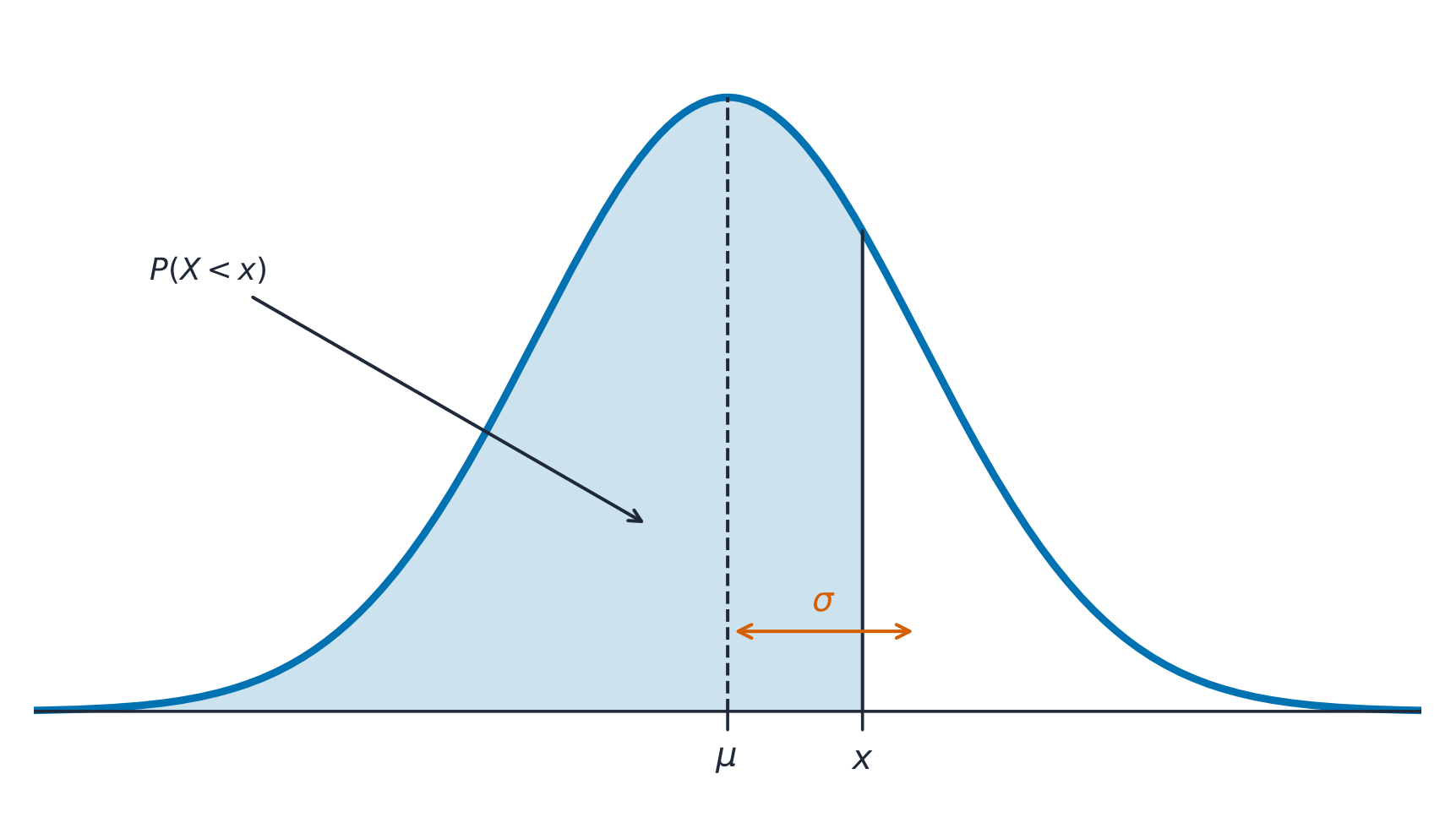
The normal curve: a probability is the area under it, centred on the mean
A $z$-score 标准分数 measures how many standard deviations a value is from the mean:
$$z=\frac{x-\mu}{\sigma}.$$
Convert to a $z$-score, then use the normal table or technology to find the proportion (area) below, above, or between values – and reverse the process to find a value from a given percentile.
Worked example. Test scores are normal with $\mu=500$ and $\sigma=100$. A score of $700$ has $z=\dfrac{700-500}{100}=2$. By the empirical rule, $95\%$ of scores lie within $2\sigma$, so $2.5\%$ lie above $700$ – meaning a $700$ is at about the $97.5$th percentile.
The normal curve and the 68-95-99.7 empirical rule
Explore · Khám phá
Explore area under the normal curve · Khám phá diện tích dưới đường cong chuẩn
The proportion of data below a value equals the area under the curve to its left. Shade a tail or a central band to see the 68–95–99.7 empirical rule and read a $z$-score as an area. · Tỷ lệ dữ liệu nhỏ hơn một giá trị bằng diện tích dưới đường cong ở bên trái giá trị đó. tô đậm một đuôi hay một dải trung tâm để thấy quy tắc thực nghiệm 68–95–99.7 và đọc một điểm $z$ như một diện tích.
Enduring Understanding (VAR-1): Given that variation may be random or not, conclusions are uncertain.
Learning Objective VAR-1.D: Identify questions to be answered about possible relationships in data. [Skill 1.A]
VAR-1.D.1 Apparent patterns and associations in data may be random or not.
Tiếng Việt
Hiểu biết bền vững (VAR-1): Vì sự biến thiên có thể ngẫu nhiên hoặc không, nên những kết luận đều mang tính bất định.
Mục tiêu học tập VAR-1.D: Xác định các câu hỏi cần trả lời về các mối quan hệ tiềm năng trong dữ liệu. [Kỹ năng 1.A]
VAR-1.D.1 Các mẫu hình và mối liên hệ rõ ràng trong dữ liệu có thể mang tính ngẫu nhiên hoặc không.
Source: College Board AP Course and Exam Description · Nguồn: Mô tả Khóa học và Bài thi College Board AP
Two-variable data let us ask whether two characteristics are associated 关联 – whether knowing one tells you something about the other. An explanatory variable 解释变量 (the "input") may help predict a response variable 响应变量 (the "output"). Association is not the same as causation.
Enduring Understanding (UNC-1): Graphical representations and statistics allow us to identify and represent key features of data.
Learning Objective UNC-1.P: Compare numerical and graphical representations for two categorical variables. [Skill 2.D]
UNC-1.P.1 Side-by-side bar graphs, segmented bar graphs, and mosaic plots are examples of bar graphs for one categorical variable, broken down by categories of another categorical variable.
UNC-1.P.2 Graphical representations of two categorical variables can be used to compare distributions and/or determine if variables are associated.
UNC-1.P.3 A two-way table, also called a contingency table, is used to summarize two categorical variables. The entries in the cells can be frequency counts or relative frequencies.
UNC-1.P.4 A joint relative frequency is a cell frequency divided by the total for the entire table.
Tiếng Việt
Hiểu biết bền vững (UNC-1): Các biểu đồ và số liệu thống kê giúp chúng ta xác định và biểu diễn các đặc điểm chính của dữ liệu.
Mục tiêu học tập UNC-1.P: So sánh các biểu diễn số và đồ thị cho hai biến định tính. [Kỹ năng 2.D]
UNC-1.P.1 Biểu đồ cột đặt cạnh nhau, biểu đồ cột phân đoạn, và biểu đồ mosaic là các ví dụ về biểu đồ cột cho một biến định tính, được phân tách theo các danh mục của một biến định tính khác.
UNC-1.P.2 Các biểu diễn đồ thị của hai biến định tính có thể được sử dụng để so sánh các phân phối và/hoặc xác định xem các biến có liên quan với nhau hay không.
UNC-1.P.3 Bảng hai chiều, còn gọi là bảng liên hệ, được sử dụng để tóm tắt hai biến phân loại. Các ô trong bảng có thể chứa số liệu tần suất hoặc tần suất tương đối.
UNC-1.P.4 Tần suất tương đối chung là tần suất của một ô chia cho tổng số của toàn bộ bảng.
Source: College Board AP Course and Exam Description · Nguồn: Mô tả Khóa học và Bài thi College Board AP
A two-way table 双向表 (contingency table) counts individuals by two categorical variables at once. A marginal distribution 边缘分布 is a row or column total written as a fraction of the grand total (the totals themselves are just counts). Comparing the inside cells shows whether the variables are related.
Enduring Understanding (UNC-1): Graphical representations and statistics allow us to identify and represent key features of data.
Learning Objective UNC-1.Q: Calculate statistics for two categorical variables. [Skill 2.C]
UNC-1.Q.1 The marginal relative frequencies are the row and column totals in a two-way table divided by the total for the entire table.
UNC-1.Q.2 A conditional relative frequency is a relative frequency for a specific part of the contingency table (e.g., cell frequencies in a row divided by the total for that row).
Learning Objective UNC-1.R: Compare statistics for two categorical variables. [Skill 2.D]
UNC-1.R.1 Summary statistics for two categorical variables can be used to compare distributions and/or determine if variables are associated.
Tiếng Việt
Hiểu biết bền vững (UNC-1): Các biểu đồ và số liệu thống kê giúp chúng ta xác định và biểu diễn các đặc điểm chính của dữ liệu.
Mục tiêu học tập UNC-1.Q: Tính toán thống kê cho hai biến phân loại. [Kỹ năng 2.C]
UNC-1.Q.1 Tần suất tương đối biên là tổng các hàng và cột trong bảng hai chiều chia cho tổng số của toàn bộ bảng.
UNC-1.Q.2 Tần suất tương đối điều kiện là tần suất tương đối của một phần cụ thể trong bảng liên hệ (ví dụ: tần suất ô trong một hàng chia cho tổng số của hàng đó).
Mục tiêu học tập UNC-1.R: So sánh thống kê cho hai biến phân loại. [Kỹ năng 2.D]
UNC-1.R.1 Các thống kê tóm tắt cho hai biến phân loại có thể được sử dụng để so sánh phân phối và/hoặc xác định xem các biến có liên quan với nhau hay không.
Source: College Board AP Course and Exam Description · Nguồn: Mô tả Khóa học và Bài thi College Board AP
A conditional distribution 条件分布 is the distribution of one variable within a fixed category of the other (found by dividing each cell by its row or column total). If the conditional distributions differ across groups, the two variables are associated; if they are the same, there is no association. Segmented bar charts 分段条形图 or mosaic plots display them.
Enduring Understanding (UNC-1): Graphical representations and statistics allow us to identify and represent key features of data.
Learning Objective UNC-1.S: Represent bivariate quantitative data using scatterplots. [Skill 2.B]
UNC-1.S.1 A bivariate quantitative data set consists of observations of two different quantitative variables made on individuals in a sample or population.
UNC-1.S.2 A scatterplot shows two numeric values for each observation, one corresponding to the value on the $x$-axis and one corresponding to the value on the $y$-axis.
UNC-1.S.3 An explanatory variable is a variable whose values are used to explain or predict corresponding values for the response variable.
Enduring Understanding (DAT-1): Regression models may allow us to predict responses to changes in an explanatory variable.
Learning Objective DAT-1.A: Describe the characteristics of a scatter plot. [Skill 2.A]
DAT-1.A.1 A description of a scatter plot includes form, direction, strength, and unusual features.
DAT-1.A.2 The direction of the association shown in a scatterplot, if any, can be described as positive or negative.
DAT-1.A.3 A positive association means that as values of one variable increase, the values of the other variable tend to increase. A negative association means that as values of one variable increase, values of the other variable tend to decrease.
DAT-1.A.4 The form of the association shown in a scatterplot, if any, can be described as linear or non-linear to varying degrees.
DAT-1.A.5 The strength of the association is how closely the individual points follow a specific pattern, e.g., linear, and can be shown in a scatterplot. Strength can be described as strong, moderate, or weak.
DAT-1.A.6 Unusual features of a scatter plot include clusters of points or points with relatively large discrepancies between the value of the response variable and a predicted value for the response variable.
Tiếng Việt
Hiểu biết bền vững (UNC-1): Các biểu đồ và số liệu thống kê giúp chúng ta xác định và biểu diễn các đặc điểm chính của dữ liệu.
Mục tiêu học tập UNC-1.S: Biểu diễn dữ liệu định lượng hai biến bằng biểu đồ phân tán. [Kỹ năng 2.B]
UNC-1.S.1 Một tập dữ liệu định lượng hai biến bao gồm các quan sát của hai biến định lượng khác nhau trên các cá thể trong một mẫu hoặc quần thể.
UNC-1.S.2 Biểu đồ phân tán hiển thị hai giá trị số cho mỗi quan sát, một giá trị tương ứng với giá trị trên trục $x$ và một giá trị tương ứng với giá trị trên trục $y$.
UNC-1.S.3 Biến giải thích là biến mà các giá trị của nó được sử dụng để giải thích hoặc dự đoán các giá trị tương ứng của biến phản hồi.
Hiểu biết cốt lõi (DAT-1): Các mô hình hồi quy có thể cho phép chúng ta dự đoán phản hồi trước những thay đổi của biến giải thích.
Mục tiêu học tập DAT-1.A: Mô tả các đặc điểm của biểu đồ phân tán. [Kỹ năng 2.A]
DAT-1.A.1 Một mô tả về biểu đồ phân tán bao gồm hình dạng, hướng, độ mạnh và các đặc điểm bất thường.
DAT-1.A.2 Hướng của mối liên hệ được hiển thị trong biểu đồ phân tán, nếu có, có thể được mô tả là dương tính hoặc âm tính.
DAT-1.A.3 Mối liên hệ dương tính có nghĩa là khi giá trị của một biến tăng lên, giá trị của biến kia cũng có xu hướng tăng lên. Mối liên hệ âm tính có nghĩa là khi giá trị của một biến tăng lên, giá trị của biến kia có xu hướng giảm xuống.
DAT-1.A.4 Hình dạng của mối liên hệ được hiển thị trong biểu đồ phân tán, nếu có, có thể được mô tả là tuyến tính hoặc phi tuyến tính ở mức độ khác nhau.
DAT-1.A.5 Độ mạnh của mối liên hệ là mức độ các điểm riêng lẻ tuân theo một mẫu cụ thể, ví dụ như tuyến tính, và có thể được thể hiện trong biểu đồ phân tán. Độ mạnh có thể được mô tả là mạnh, trung bình hoặc yếu.
DAT-1.A.6 Các đặc điểm bất thường của biểu đồ phân tán bao gồm các cụm điểm hoặc các điểm có sự chênh lệch tương đối lớn giữa giá trị của biến phản hồi và giá trị dự đoán cho biến phản hồi đó.
Source: College Board AP Course and Exam Description · Nguồn: Mô tả Khóa học và Bài thi College Board AP
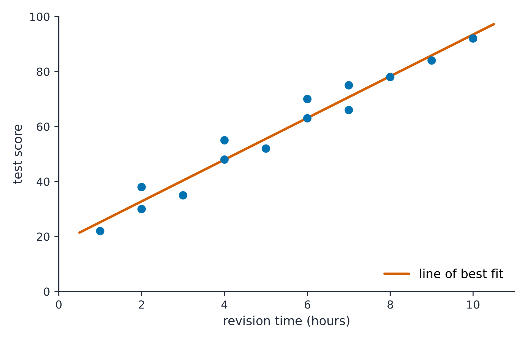
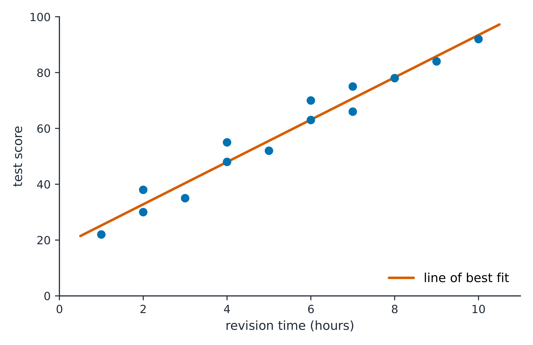
A scatterplot 散点图 plots each individual as a point, explanatory variable on the $x$-axis and response on the $y$-axis. Describe it with DUFS: Direction (positive/negative), Unusual features (outliers, clusters), Form (linear or curved), and Strength (how tightly the points follow the pattern) – always in context.
A line of best fit runs through the middle of the scattered points
Enduring Understanding (DAT-1): Regression models may allow us to predict responses to changes in an explanatory variable.
Learning Objective DAT-1.B: Determine the correlation for a linear relationship. [Skill 2.C]
DAT-1.B.1 The correlation, $r$, gives the direction and quantifies the strength of the linear association between two quantitative variables.
DAT-1.B.2 The correlation coefficient can be calculated by: $r = \dfrac{1}{n-1} \sum \left( \dfrac{x_i - \bar{x}}{s_x} \right) \left( \dfrac{y_i - \bar{y}}{s_y} \right)$. However, the most common way to determine $r$ is by using technology.
DAT-1.B.3 A correlation coefficient close to 1 or $-1$ does not necessarily mean that a linear model is appropriate.
Learning Objective DAT-1.C: Interpret the correlation for a linear relationship. [Skill 4.B]
DAT-1.C.1 The correlation, $r$, is unit-free, and always between $-1$ and 1, inclusive. A value of $r = 0$ indicates that there is no linear association. A value of $r = 1$ or $r = -1$ indicates that there is a perfect linear association.
DAT-1.C.2 A perceived or real relationship between two variables does not mean that changes in one variable cause changes in the other. That is, correlation does not necessarily imply causation.
Tiếng Việt
Hiểu biết cốt lõi (DAT-1): Các mô hình hồi quy có thể cho phép chúng ta dự đoán phản hồi trước những thay đổi của biến giải thích.
Mục tiêu học tập DAT-1.B: Xác định hệ số tương quan cho mối quan hệ tuyến tính. [Kỹ năng 2.C]
DAT-1.B.1 Hệ số tương quan, $r$, cho biết hướng và định lượng độ mạnh của mối liên hệ tuyến tính giữa hai biến định lượng.
DAT-1.B.2 Hệ số tương quan có thể được tính bằng: $r = \dfrac{1}{n-1} \sum \left( \dfrac{x_i - \bar{x}}{s_x} \right) \left( \dfrac{y_i - \bar{y}}{s_y} \right)$. Tuy nhiên, cách phổ biến nhất để xác định $r$ là sử dụng công nghệ.
DAT-1.B.3 Một hệ số tương quan gần 1 hoặc $-1$ không nhất thiết có nghĩa là mô hình tuyến tính là phù hợp.
Mục tiêu học tập DAT-1.C: Giải thích hệ số tương quan cho mối quan hệ tuyến tính. [Kỹ năng 4.B]
DAT-1.C.1 Hệ số tương quan, $r$, không có đơn vị và luôn nằm trong khoảng từ $-1$ đến 1, bao gồm cả hai giá trị biên. Giá trị $r = 0$ cho thấy không có mối liên hệ tuyến tính. Giá trị $r = 1$ hoặc $r = -1$ cho thấy có mối liên hệ tuyến tính hoàn hảo.
DAT-1.C.2 Một mối quan hệ cảm nhận hoặc thực tế giữa hai biến không có nghĩa là sự thay đổi của một biến gây ra sự thay đổi của biến kia. Nói cách khác, tương quan không nhất thiết ngụ ý nguyên nhân - kết quả.
Source: College Board AP Course and Exam Description · Nguồn: Mô tả Khóa học và Bài thi College Board AP
What r actually measures
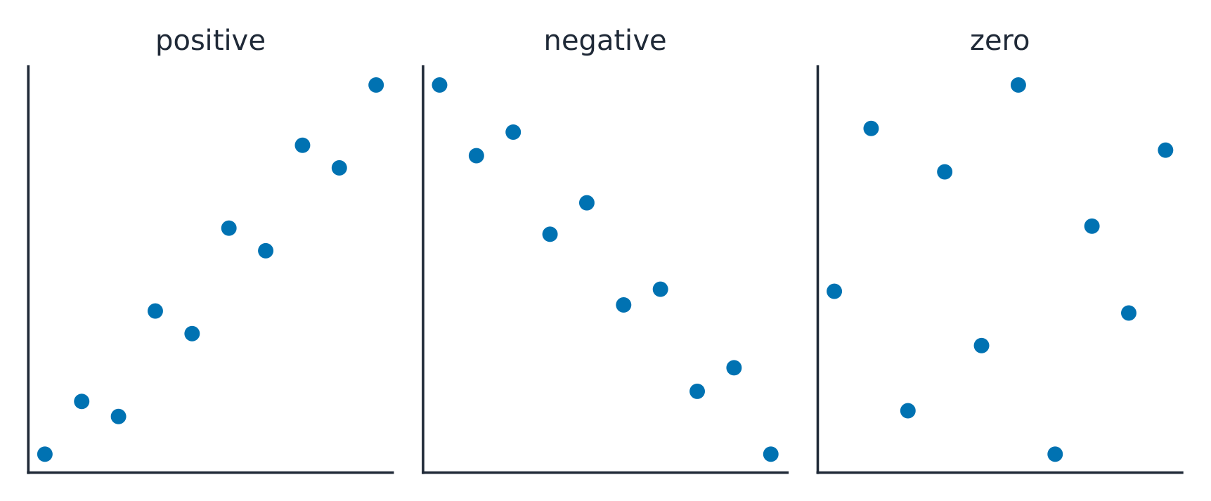
The correlation coefficient 相关系数$r$ measures the strength and direction of a linear relationship. It runs from $-1$ to $1$: near $\pm 1$ is strong linear, near $0$ is weak linear. $r$ has no units and does not change if you swap the variables. Warnings: $r$ only measures linear strength, it is not resistant to outliers, and a strong $r$ does not prove causation.
Positive correlation rises together; negative correlation moves in opposite directions
Explore · Khám phá
Strength of a linear relationship · Cường độ mối quan hệ tuyến tính
Correlation$r$ runs from $-1$ to $1$: near $\pm1$ the points hug a line, near 0 they scatter. Change it and watch the cloud tighten or spread. · Hệ số tương quan$r$ chạy từ $-1$ đến $1$: gần $\pm1$, các điểm bám sát đường thẳng; gần 0, chúng phân tán rời rạc. Thay đổi giá trị này và quan sát đám mây điểm thu hẹp lại hay mở rộng ra.
Enduring Understanding (DAT-1): Regression models may allow us to predict responses to changes in an explanatory variable.
Learning Objective DAT-1.D: Calculate a predicted response value using a linear regression model. [Skill 2.C]
DAT-1.D.1 A simple linear regression model is an equation that uses an explanatory variable, $x$, to predict the response variable, $y$.
DAT-1.D.2 The predicted response value, denoted by $\hat{y}$, is calculated as $\hat{y} = a + bx$, where $a$ is the $y$-intercept and $b$ is the slope of the regression line, and $x$ is the value of the explanatory variable.
DAT-1.D.3 Extrapolation is predicting a response value using a value for the explanatory variable that is beyond the interval of $x$-values used to determine the regression line. The predicted value is less reliable as an estimate the further we extrapolate.
Tiếng Việt
Hiểu biết cốt lõi (DAT-1): Các mô hình hồi quy có thể cho phép chúng ta dự đoán phản hồi trước những thay đổi của biến giải thích.
Mục tiêu học tập DAT-1.D: Tính toán giá trị dự đoán bằng mô hình hồi quy tuyến tính. [Kỹ năng 2.C]
DAT-1.D.1 Một mô hình hồi quy tuyến tính đơn giản là một phương trình sử dụng biến giải thích, $x$, để dự đoán biến phản hồi, $y$.
DAT-1.D.2 Giá trị dự đoán, ký hiệu bởi $\hat{y}$, được tính bằng $\hat{y} = a + bx$, trong đó $a$ là giao điểm trên trục $y$ và $b$ là độ dốc của đường hồi quy, và $x$ là giá trị của biến giải thích.
DAT-1.D.3 Ngoại suy là dự đoán một giá trị phản hồi bằng cách sử dụng một giá trị của biến giải thích nằm ngoài khoảng các giá trị $x$ được sử dụng để xác định đường hồi quy. Giá trị dự đoán kém đáng tin cậy hơn như một ước lượng khi chúng ta ngoại suy càng xa.
Source: College Board AP Course and Exam Description · Nguồn: Mô tả Khóa học và Bài thi College Board AP
The least-squares regression line 最小二乘回归线 predicts the response: $\hat{y}=a+bx$, where $\hat{y}$ is the predicted response. The slope 斜率$b$ is the predicted change in $y$ per one-unit increase in $x$; the $y$-intercept 截距$a$ is the predicted $y$ when $x=0$. Interpret both in context and with units – a graded skill. Avoid extrapolation 外推 (predicting far outside the data).
Worked example. A study of hours studied ($x$) and test score ($y$) gives $\hat{y}=20+3x$. The slope means each extra hour of study is associated with a predicted $3$-point increase. A student who studies $5$ hours is predicted to score $\hat{y}=20+3(5)=35$.
Explore · Khám phá
Fit a least-squares line · Vẽ đường hồi quy bình phương tối thiểu
A regression line is the best straight-line fit, minimising the squared vertical distances. Its slope predicts how $y$ changes per unit of $x$. · Một đường hồi quy là đường thẳng phù hợp tốt nhất, tối thiểu hóa tổng bình phương các khoảng cách dọc. Hệ số góc của nó dự đoán sự thay đổi của $y$ theo mỗi đơn vị của $x$.
Enduring Understanding (DAT-1): Regression models may allow us to predict responses to changes in an explanatory variable.
Learning Objective DAT-1.E: Represent differences between measured and predicted responses using residual plots. [Skill 2.B]
DAT-1.E.1 The residual is the difference between the actual value and the predicted value: $\text{residual} = y - \hat{y}$.
DAT-1.E.2 A residual plot is a plot of residuals versus explanatory variable values or predicted response values.
Learning Objective DAT-1.F: Describe the form of association of bivariate data using residual plots. [Skill 2.A]
DAT-1.F.1 Apparent randomness in a residual plot for a linear model is evidence of a linear form to the association between the variables.
DAT-1.F.2 Residual plots can be used to investigate the appropriateness of a selected model.
Tiếng Việt
Hiểu biết cốt lõi (DAT-1): Các mô hình hồi quy có thể cho phép chúng ta dự đoán phản hồi trước những thay đổi của biến giải thích.
Mục tiêu học tập DAT-1.E: Biểu diễn sự khác biệt giữa các giá trị đo lường và giá trị dự đoán bằng biểu đồ phần dư. [Kỹ năng 2.B]
DAT-1.E.1 Phần dư là sự khác biệt giữa giá trị thực tế và giá trị dự đoán: $\text{residual} = y - \hat{y}$.
DAT-1.E.2 Biểu đồ phần dư là biểu đồ của các phần dư theo các giá trị của biến giải thích hoặc các giá trị phản hồi dự đoán.
Mục tiêu học tập DAT-1.F: Mô tả hình dạng của mối liên hệ trong dữ liệu hai biến bằng biểu đồ phần dư. [Kỹ năng 2.A]
DAT-1.F.1 Sự ngẫu nhiên rõ ràng trong biểu đồ phần dư của một mô hình tuyến tính là bằng chứng cho thấy hình dạng tuyến tính của mối liên hệ giữa các biến.
DAT-1.F.2 Biểu đồ phần dư có thể được sử dụng để kiểm tra tính phù hợp của một mô hình đã chọn.
Source: College Board AP Course and Exam Description · Nguồn: Mô tả Khóa học và Bài thi College Board AP
Least-squares regression
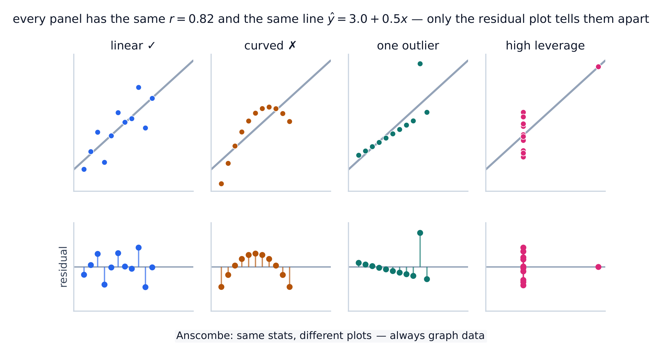
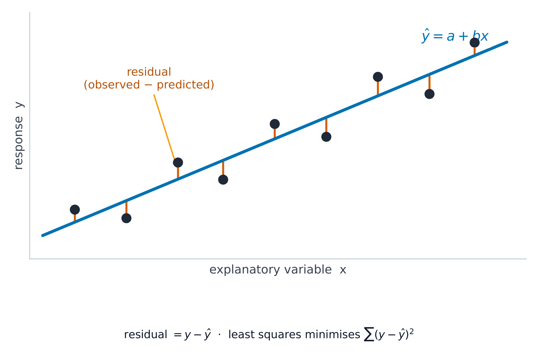
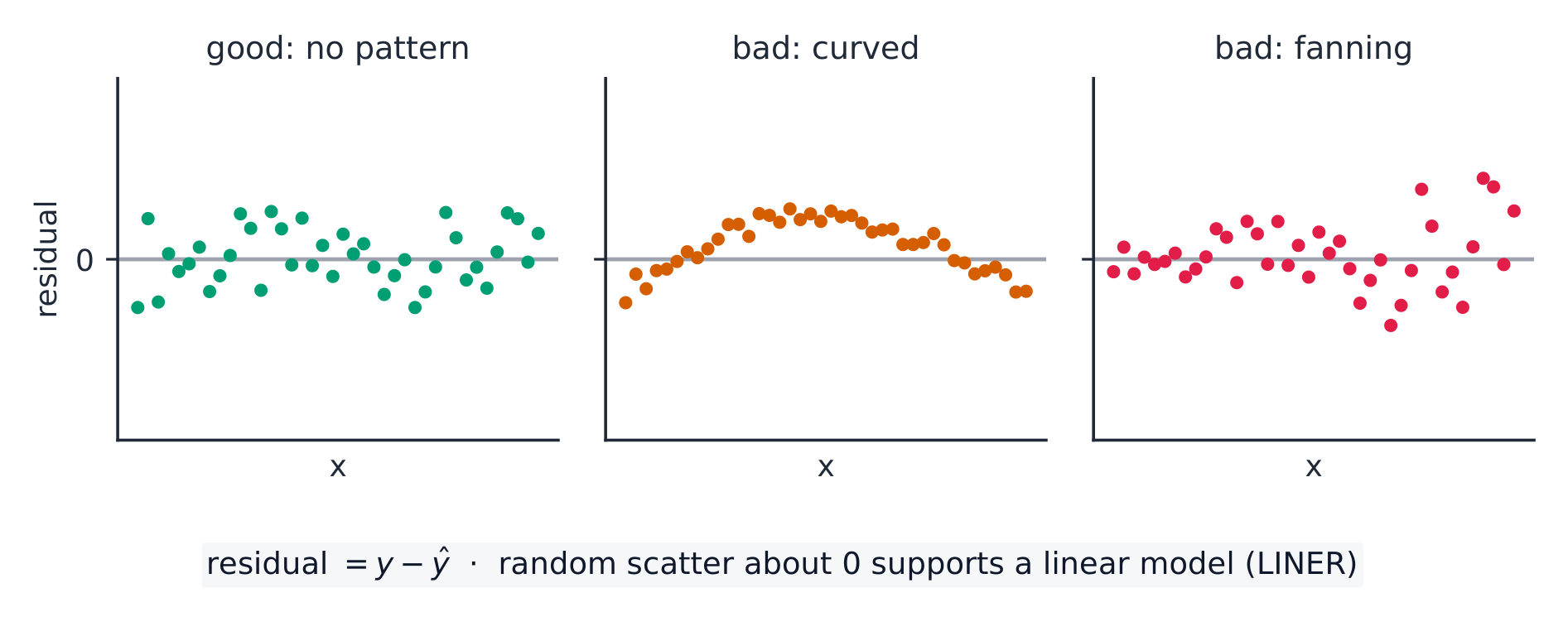
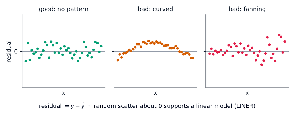
A residual 残差 is actual minus predicted, $y-\hat{y}$: how far a point sits above (+) or below (−) the line. A residual plot 残差图 graphs residuals against $x$. If it shows no pattern (random scatter), a linear model is appropriate; a curved or fanning pattern means the linear model is a poor fit.
Worked example. Continuing the study above, a student who studied $5$ hours actually scored $40$. The residual is $y-\hat{y}=40-35=+5$: the line under-predicted by $5$ points, so this point sits above the line.
A caution about $r$ and the line: all four datasets have the same $r=0.82$ and the same $\hat{y}=3.0+0.5x$, yet only the first is genuinely linear. The scatterplots barely differ — the residual plot below each is what exposes the curve, the outlier, and the high-leverage point.
Enduring Understanding (DAT-1): Regression models may allow us to predict responses to changes in an explanatory variable.
Learning Objective DAT-1.G: Estimate parameters for the least-squares regression line model. [Skill 2.C]
DAT-1.G.1 The least-squares regression model minimizes the sum of the squares of the residuals and contains the point $(\bar{x}, \bar{y})$.
DAT-1.G.2 The slope, $b$, of the regression line can be calculated as $b = r \left( \dfrac{s_y}{s_x} \right)$ where $r$ is the correlation between $x$ and $y$, $s_y$ is the sample standard deviation of the response variable, $y$, and $s_x$ is the sample standard deviation of the explanatory variable, $x$.
DAT-1.G.3 Sometimes, the $y$-intercept of the line does not have a logical interpretation in context.
DAT-1.G.4 In simple linear regression, $r^2$ is the square of the correlation, $r$. It is also called the coefficient of determination. $r^2$ is the proportion of variation in the response variable that is explained by the explanatory variable in the model.
Learning Objective DAT-1.H: Interpret coefficients for the least-squares regression line model. [Skill 4.B]
DAT-1.H.1 The coefficients of the least-squares regression model are the estimated slope and $y$-intercept.
DAT-1.H.2 The slope is the amount that the predicted $y$-value changes for every unit increase in $x$.
DAT-1.H.3 The $y$-intercept value is the predicted value of the response variable when the explanatory variable is equal to $0$. The formula for the $y$-intercept, $a$, is $a = \bar{y} - b\bar{x}$.
Tiếng Việt
Hiểu biết cốt lõi (DAT-1): Các mô hình hồi quy có thể cho phép chúng ta dự đoán phản hồi trước những thay đổi của biến giải thích.
Mục tiêu học tập DAT-1.G: Ước lượng tham số cho mô hình đường hồi quy bình phương tối thiểu. [Kỹ năng 2.C]
DAT-1.G.1 Mô hình hồi quy bình phương tối thiểu tối thiểu hóa tổng bình phương phần dư và chứa điểm $(\bar{x}, \bar{y})$.
DAT-1.G.2 Hệ số góc, $b$, của đường hồi quy có thể được tính theo công thức $b = r \left( \dfrac{s_y}{s_x} \right)$, trong đó $r$ là hệ số tương quan giữa $x$ và $y$, $s_y$ là độ lệch chuẩn mẫu của biến phản ứng, $y$, và $s_x$ là độ lệch chuẩn mẫu của biến giải thích, $x$.
DAT-1.G.3 Đôi khi, $y$-trục (trục tung) của đường thẳng không có ý nghĩa thực tế trong ngữ cảnh.
DAT-1.G.4 Trong hồi quy tuyến tính đơn giản, $r^2$ là bình phương của hệ số tương quan, $r$. Nó còn được gọi là hệ số xác định. $r^2$ là tỷ lệ biến thiên của biến phản ứng được giải thích bởi biến giải thích trong mô hình.
Mục tiêu học tập DAT-1.H: Giải thích các hệ số của mô hình đường hồi quy bình phương tối thiểu. [Kỹ năng 4.B]
DAT-1.H.1 Các hệ số của mô hình hồi quy bình phương tối thiểu là độ dốc ước lượng và $y$-trục (trục tung).
DAT-1.H.2 Hệ số góc là mức thay đổi của giá trị dự báo $y$ đối với mỗi đơn vị gia tăng của $x$.
DAT-1.H.3 Giá trị $y$-trục (trục tung) là giá trị dự báo của biến phản hồi khi biến giải thích bằng $0$. Công thức cho $y$-trục (trục tung), $a$, là $a = \bar{y} - b\bar{x}$.
Source: College Board AP Course and Exam Description · Nguồn: Mô tả Khóa học và Bài thi College Board AP
The least-squares line minimizes the sum of squared residuals
The line minimizes the sum of squared residuals. Its fit is measured by:
$s$, the standard deviation of the residuals – the typical prediction error, in the response's units.
$r^2$, the coefficient of determination 决定系数 – the proportion of the variation in $y$ that the linear model explains (a value between $0$ and $1$; multiply by $100$ to state it as a percent). Report it in context: "$r^2 = 0.81$ means 81% of the variation in $y$ is explained by the linear relationship with $x$."
coefficient of determination/ˌkəʊɪˈfɪʃənt ɒv dɪˌtɜːmɪˈneɪʃn/
hệ số xác định
2.9
Departures from Linearity
Syllabus · Chương trình
English
Enduring Understanding (DAT-1): Regression models may allow us to predict responses to changes in an explanatory variable.
Learning Objective DAT-1.I: Identify influential points in regression. [Skill 2.A]
DAT-1.I.1 An outlier in regression is a point that does not follow the general trend shown in the rest of the data and has a large residual when the Least Squares Regression Line (LSRL) is calculated.
DAT-1.I.2 A high-leverage point in regression has a substantially larger or smaller $x$-value than the other observations have.
DAT-1.I.3 An influential point in regression is any point that, if removed, changes the relationship substantially. Examples include much different slope, $y$-intercept, and/or correlation. Outliers and high leverage points are often influential.
Learning Objective DAT-1.J: Calculate a predicted response using a least-squares regression line for a transformed data set. [Skill 2.C]
DAT-1.J.1 Transformations of variables, such as evaluating the natural logarithm of each value of the response variable or squaring each value of the explanatory variable, can be used to create transformed data sets, which may be more linear in form than the untransformed data.
DAT-1.J.2 Increased randomness in residual plots after transformation of data and/or movement of $r^2$ to a value closer to 1 offers evidence that the least-squares regression line for the transformed data is a more appropriate model to use to predict responses to the explanatory variable than the regression line for the untransformed data.
Tiếng Việt
Hiểu biết cốt lõi (DAT-1): Các mô hình hồi quy có thể cho phép chúng ta dự đoán phản hồi trước những thay đổi của biến giải thích.
Mục tiêu học tập DAT-1.I: Xác định các điểm ảnh hưởng trong hồi quy. [Kỹ năng 2.A]
DAT-1.I.1 Một điểm ngoại lai trong hồi quy là một điểm không tuân theo xu hướng chung được thể hiện ở phần dữ liệu còn lại và có phần dư lớn khi Đường hồi quy bình phương tối thiểu (LSRL) được tính toán.
DAT-1.I.2 Một điểm có sức nặng cao (high-leverage point) trong hồi quy có giá trị $x$ lớn hơn hoặc nhỏ hơn đáng kể so với các quan sát khác.
DAT-1.I.3 Một điểm ảnh hưởng trong hồi quy là bất kỳ điểm nào mà nếu bị loại bỏ sẽ làm thay đổi mối quan hệ đáng kể. Ví dụ bao gồm độ dốc khác biệt nhiều, $y$-trục (trục tung), và/hoặc tương quan. Điểm ngoại lai và điểm có lực cao thường mang tính ảnh hưởng.
Mục tiêu học tập DAT-1.J: Tính giá trị dự báo sử dụng đường hồi quy bình phương tối thiểu cho bộ dữ liệu đã được biến đổi. [Kỹ năng 2.C]
DAT-1.J.1 Việc biến đổi các biến, chẳng hạn như tính logarit tự nhiên của từng giá trị của biến phản ứng hoặc bình phương từng giá trị của biến giải thích, có thể được sử dụng để tạo ra các bộ dữ liệu đã biến đổi, vốn có dạng tuyến tính hơn so với dữ liệu chưa biến đổi.
DAT-1.J.2 Sự tăng lên của tính ngẫu nhiên trong biểu đồ phần dư sau khi biến đổi dữ liệu và/hoặc việc di chuyển $r^2$ đến một giá trị gần 1 hơn cung cấp bằng chứng cho thấy đường hồi quy bình phương tối thiểu của dữ liệu đã biến đổi là mô hình phù hợp hơn để dự báo các phản ứng đối với biến giải thích so với đường hồi quy của dữ liệu chưa biến đổi.
Source: College Board AP Course and Exam Description · Nguồn: Mô tả Khóa học và Bài thi College Board AP
Some points strongly affect the line. A high-leverage 高杠杆 point has an extreme $x$-value; an influential 有影响的 point noticeably changes the slope or $r$ when removed; an outlier here is a point with a large residual. When the pattern is curved, transform a variable (e.g. take a log) to straighten it, then fit a line to the transformed data.
Enduring Understanding (VAR-1): Given that variation may be random or not, conclusions are uncertain.
Learning Objective VAR-1.E: Identify questions to be answered about data collection methods. [Skill 1.A]
VAR-1.E.1 Methods for data collection that do not rely on chance result in untrustworthy conclusions.
Tiếng Việt
Hiểu biết bền vững (VAR-1): Vì sự biến thiên có thể ngẫu nhiên hoặc không, nên những kết luận đều mang tính bất định.
Mục tiêu học tập VAR-1.E: Xác định các câu hỏi cần trả lời về phương pháp thu thập dữ liệu. [Kỹ năng 1.A]
VAR-1.E.1 Các phương pháp thu thập dữ liệu không dựa trên yếu tố ngẫu nhiên dẫn đến kết luận không đáng tin cậy.
Source: College Board AP Course and Exam Description · Nguồn: Mô tả Khóa học và Bài thi College Board AP
A conclusion is only as good as the data behind it. How data are collected decides what you may conclude – whether you can generalize to a population 总体, and whether you can claim cause and effect. Poorly collected data can be worse than none.
Enduring Understanding (DAT-2): The way we collect data influences what we can and cannot say about a population.
Learning Objective DAT-2.A: Identify the type of a study. [Skill 1.C]
DAT-2.A.1 A population consists of all items or subjects of interest.
DAT-2.A.2 A sample selected for study is a subset of the population.
DAT-2.A.3 In an observational study, treatments are not imposed. Investigators examine data for a sample of individuals (retrospective) or follow a sample of individuals into the future collecting data (prospective) in order to investigate a topic of interest about the population. A sample survey is a type of observational study that collects data from a sample in an attempt to learn about the population from which the sample was taken.
DAT-2.A.4 In an experiment, different conditions (treatments) are assigned to experimental units (participants or subjects).
Learning Objective DAT-2.B: Identify appropriate generalizations and determinations based on observational studies. [Skill 4.A]
DAT-2.B.1 It is only appropriate to make generalizations about a population based on samples that are randomly selected or otherwise representative of that population.
DAT-2.B.2 A sample is only generalizable to the population from which the sample was selected.
DAT-2.B.3 It is not possible to determine causal relationships between variables using data collected in an observational study.
Tiếng Việt
Hiểu biết bền vững (DAT-2): Cách chúng ta thu thập dữ liệu ảnh hưởng đến những gì chúng ta có thể và không thể nói về một quần thể.
Mục tiêu học tập DAT-2.A: Xác định loại hình nghiên cứu. [Kỹ năng 1.C]
DAT-2.A.1 Một quần thể bao gồm tất cả các đối tượng hoặc chủ thể quan tâm.
DAT-2.A.2 Một mẫu được chọn để nghiên cứu là một tập con của quần thể.
DAT-2.A.3 Trong nghiên cứu quan sát, các điều trị không được áp đặt. Các nhà nghiên cứu xem xét dữ liệu từ một mẫu cá nhân (hồi cứu) hoặc theo dõi một mẫu cá nhân vào tương lai để thu thập dữ liệu (tiên tiến) nhằm khám phá một chủ đề quan tâm về quần thể. Khảo sát mẫu là một loại nghiên cứu quan sát thu thập dữ liệu từ một mẫu nhằm tìm hiểu về quần thể mà mẫu đó được抽取 từ.
DAT-2.A.4 Trong thí nghiệm, các điều kiện khác nhau (điều trị) được gán cho các đơn vị thí nghiệm (tham gia viên hoặc chủ thể).
Mục tiêu học tập DAT-2.B: Xác định các khái quát hóa và kết luận thích hợp dựa trên các nghiên cứu quan sát. [Kỹ năng 4.A]
DAT-2.B.1 Chỉ thích hợp khi đưa ra các khái quát hóa về một quần thể dựa trên các mẫu được chọn ngẫu nhiên hoặc đại diện cho quần thể đó.
DAT-2.B.2 Một mẫu chỉ có thể khái quát hóa sang quần thể mà từ đó mẫu được chọn.
DAT-2.B.3 Không thể xác định các mối quan hệ nguyên nhân - kết quả giữa các biến sử dụng dữ liệu thu thập được từ một nghiên cứu quan sát.
Source: College Board AP Course and Exam Description · Nguồn: Mô tả Khóa học và Bài thi College Board AP
In an observational study 观察性研究 you measure individuals without trying to influence them. It can show association, but not causation, because lurking variables may explain the link.
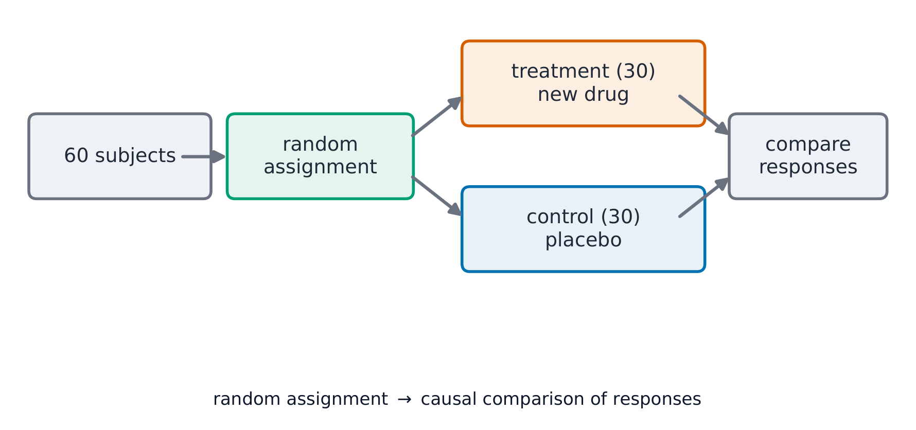
In an experiment 实验 you deliberately impose a treatment 处理 and compare responses. A well-designed experiment can establish cause and effect.
Explore · Khám phá
Observational study or experiment? · Nghiên cứu quan sát hay thí nghiệm?
In an experiment the researcher imposes a treatment (and can show cause); an observational study only records what already happens (and can show association, not cause). · Trong một thí nghiệm, nhà nghiên cứu áp đặt can thiệp (và có thể chứng minh nguyên nhân); một nghiên cứu quan sát chỉ ghi lại những gì đang xảy ra sẵn (và chỉ có thể chứng minh mối liên hệ, không phải nguyên nhân).
Enduring Understanding (DAT-2): The way we collect data influences what we can and cannot say about a population.
Learning Objective DAT-2.C: Identify a sampling method, given a description of a study. [Skill 1.C]
DAT-2.C.1 When an item from a population can be selected only once, this is called sampling without replacement. When an item from the population can be selected more than once, this is called sampling with replacement.
DAT-2.C.2 A simple random sample (SRS) is a sample in which every group of a given size has an equal chance of being chosen. This method is the basis for many types of sampling mechanisms. A few examples of mechanisms used to obtain SRSs include numbering individuals and using a random number generator to select which ones to include in the sample, ignoring repeats, using a table of random numbers, or drawing a card from a deck without replacement.
DAT-2.C.3 A stratified random sample involves the division of a population into separate groups, called strata, based on shared attributes or characteristics (homogeneous grouping). Within each stratum a simple random sample is selected, and the selected units are combined to form the sample.
DAT-2.C.4 A cluster sample involves the division of a population into smaller groups, called clusters. Ideally, there is heterogeneity within each cluster, and clusters are similar to one another in their composition. A simple random sample of clusters is selected from the population to form the sample of clusters. Data are collected from all observations in the selected clusters.
DAT-2.C.5 A systematic random sample is a method in which sample members from a population are selected according to a random starting point and a fixed, periodic interval.
DAT-2.C.6 A census selects all items/subjects in a population.
Learning Objective DAT-2.D: Explain why a particular sampling method is or is not appropriate for a given situation. [Skill 1.C]
DAT-2.D.1 There are advantages and disadvantages for each sampling method depending upon the question that is to be answered and the population from which the sample will be drawn.
Tiếng Việt
Hiểu biết bền vững (DAT-2): Cách chúng ta thu thập dữ liệu ảnh hưởng đến những gì chúng ta có thể và không thể nói về một quần thể.
Mục tiêu học tập DAT-2.C: Xác định phương pháp lấy mẫu, dựa trên mô tả về một nghiên cứu. [Kỹ năng 1.C]
DAT-2.C.1 Khi một đối tượng từ quần thể chỉ có thể được chọn một lần, điều này được gọi là lấy mẫu không hoàn lại. Khi một đối tượng từ quần thể có thể được chọn nhiều lần, điều này được gọi là lấy mẫu hoàn lại.
DAT-2.C.2 Một mẫu ngẫu nhiên đơn giản (SRS) là một mẫu trong đó mọi nhóm có kích thước cho trước đều có cơ hội ngang nhau để được chọn. Phương pháp này là nền tảng cho nhiều loại cơ chế lấy mẫu. Một vài ví dụ về các cơ chế dùng để thu được SRSs bao gồm đánh số các cá nhân và sử dụng máy phát số ngẫu nhiên để chọn những ai được đưa vào mẫu, bỏ qua các trường hợp trùng lặp, sử dụng bảng số ngẫu nhiên, hoặc rút một lá bài từ bộ bài mà không hoàn lại.
DAT-2.C.3 Mẫu ngẫu nhiên phân tầng bao gồm việc chia một tổng thể thành các nhóm riêng biệt, gọi là các tầng, dựa trên các thuộc tính hoặc đặc điểm chung (sự phân nhóm đồng nhất). Trong mỗi tầng, một mẫu ngẫu nhiên đơn được chọn, và các đơn vị được chọn được kết hợp để tạo thành mẫu.
DAT-2.C.4 Mẫu cụm bao gồm việc chia một tổng thể thành các nhóm nhỏ hơn, gọi là các cụm. Lý tưởng nhất, có sự khác biệt bên trong mỗi cụm, và các cụm tương tự nhau về cấu trúc của chúng. Một mẫu ngẫu nhiên đơn các cụm được chọn từ tổng thể để tạo thành mẫu cụm. Dữ liệu được thu thập từ tất cả các quan sát trong các cụm đã chọn.
DAT-2.C.5 Mẫu ngẫu nhiên hệ thống là phương pháp mà các thành viên mẫu từ tổng thể được chọn theo một điểm bắt đầu ngẫu nhiên và một khoảng cách định kỳ cố định.
DAT-2.C.6 Tổng điều tra chọn tất cả các mục/đối tượng trong một tổng thể.
Mục tiêu học tập DAT-2.D: Giải thích tại sao một phương pháp lấy mẫu cụ thể là phù hợp hoặc không phù hợp cho một tình huống cho trước. [Kỹ năng 1.C]
DAT-2.D.1 Mỗi phương pháp lấy mẫu đều có ưu điểm và nhược điểm tùy thuộc vào câu hỏi cần trả lời và tổng thể từ đó mẫu sẽ được抽取.
Source: College Board AP Course and Exam Description · Nguồn: Mô tả Khóa học và Bài thi College Board AP
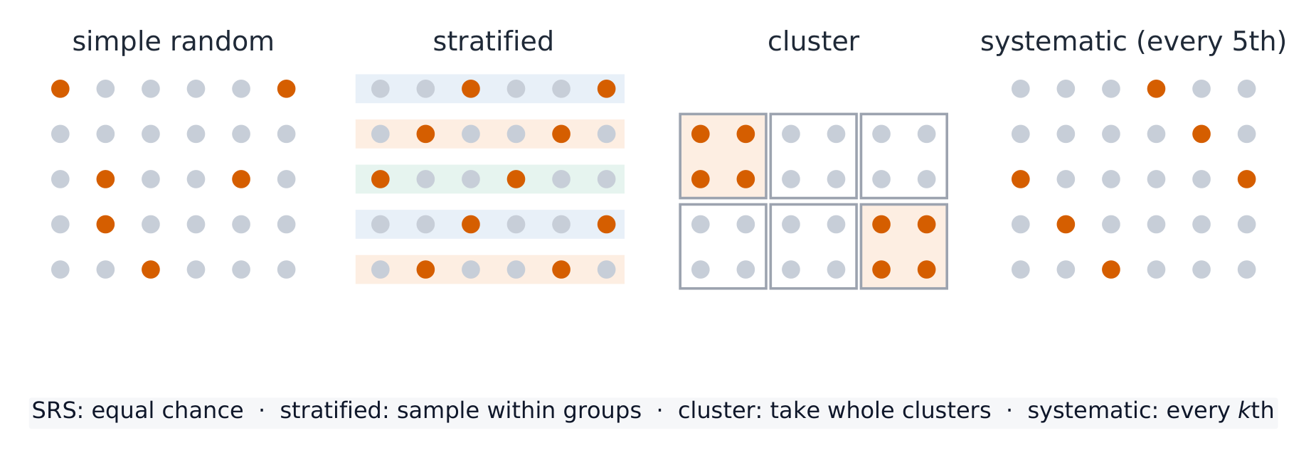
To learn about a population you take a sample 样本. Random sampling 随机抽样 protects against selection bias 偏差 and lets you generalize (it cannot fix undercoverage, nonresponse, or response bias — see below). Common designs:
Simple random sample (SRS) 简单随机样本: every group of the chosen size is equally likely.
Stratified 分层: split the population into similar strata, then sample within each.
Cluster 整群: split into clusters, randomly choose whole clusters.
Systematic 系统: pick every $k$th individual from a random start.
Four random sampling designs: who gets selected, and how
A convenience sample 方便样本 or voluntary response sample is not random and is biased.
Worked example. To survey a school, an administrator lists all students by grade and randomly selects $20$ from each grade. This is a stratified sample – the grades are the strata – which guarantees every grade is represented, unlike an SRS that might by chance draw few from one grade.
Random outcomes: dice make each face equally likely under fair conditions
Enduring Understanding (DAT-2): The way we collect data influences what we can and cannot say about a population.
Learning Objective DAT-2.E: Identify potential sources of bias in sampling methods. [Skill 1.C]
DAT-2.E.1 Bias occurs when certain responses are systematically favored over others.
DAT-2.E.2 When a sample is comprised entirely of volunteers or people who choose to participate, the sample will typically not be representative of the population (voluntary response bias).
DAT-2.E.3 When part of the population has a reduced chance of being included in the sample, the sample will typically not be representative of the population (undercoverage bias).
DAT-2.E.4 Individuals chosen for the sample for whom data cannot be obtained (or who refuse to respond) may differ from those for whom data can be obtained (nonresponse bias).
DAT-2.E.5 Problems in the data gathering instrument or process result in response bias. Examples include questions that are confusing or leading (question wording bias) and self-reported responses.
DAT-2.E.6 Non-random sampling methods (for example, samples chosen by convenience or voluntary response) introduce potential for bias because they do not use chance to select the individuals.
Tiếng Việt
Hiểu biết bền vững (DAT-2): Cách chúng ta thu thập dữ liệu ảnh hưởng đến những gì chúng ta có thể và không thể nói về một quần thể.
Mục tiêu học tập DAT-2.E: Xác định các nguồn thiên lệch tiềm tàng trong các phương pháp lấy mẫu. [Kỹ năng 1.C]
DAT-2.E.1 Thiên lệch xảy ra khi một số phản ứng được ưu tiên có hệ thống so với những phản ứng khác.
DAT-2.E.2 Khi một mẫu chỉ bao gồm những người tình nguyện hoặc những người chọn tham gia, mẫu thường sẽ không đại diện cho tổng thể (thiên lệch phản hồi tự nguyện).
DAT-2.E.3 Khi một phần của tổng thể có cơ hội thấp hơn để được đưa vào mẫu, mẫu thường sẽ không đại diện cho tổng thể (thiên lệch che phủ dưới).
DAT-2.E.4 Những cá nhân được chọn cho mẫu nhưng không thể thu thập dữ liệu (hoặc từ chối trả lời) có thể khác biệt so với những cá nhân mà dữ liệu có thể thu thập được (thiên lệch không phản hồi).
DAT-2.E.5 Các vấn đề trong dụng cụ hoặc quy trình thu thập dữ liệu dẫn đến thiên lệch phản hồi. Ví dụ bao gồm các câu hỏi gây nhầm lẫn hoặc mang tính dẫn dắt (thiên lệch cách đặt câu hỏi) và các phản hồi do chính người trả lời cung cấp.
DAT-2.E.6 Các phương pháp lấy mẫu phi ngẫu nhiên (ví dụ: mẫu chọn theo tiện lợi hoặc phản hồi tự nguyện) làm tăng khả năng xuất hiện thiên lệch vì chúng không sử dụng may mắn để chọn các cá nhân.
Source: College Board AP Course and Exam Description · Nguồn: Mô tả Khóa học và Bài thi College Board AP
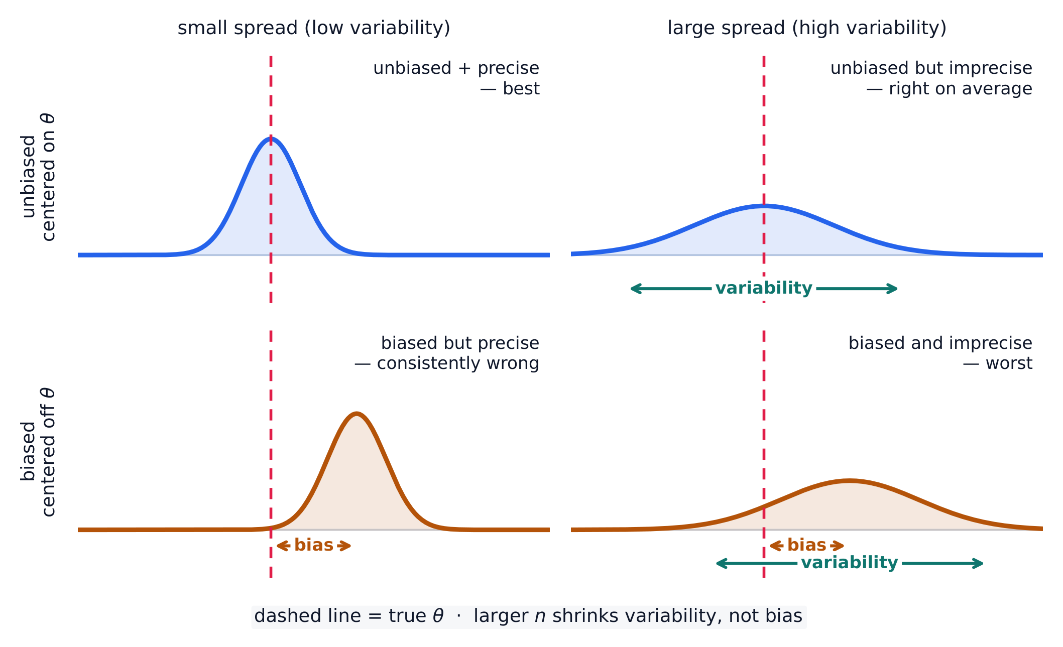
Bias makes estimates systematically miss the truth:
Undercoverage 覆盖不足: some groups are left out of the sampling frame.
Nonresponse 无回应: selected people do not answer.
Response bias 回应偏差: people answer inaccurately (bad wording, sensitive topics).
Bias is about a consistent error in one direction – increasing the sample size does not fix it.
Convenience samples miss the population: bias creeps in when selection is not random
Enduring Understanding (VAR-3): Well-designed experiments can establish evidence of causal relationships.
Learning Objective VAR-3.A: Identify the components of an experiment. [Skill 1.C]
VAR-3.A.1 The experimental units are the individuals (which may be people or other objects of study) that are assigned treatments. When experimental units consist of people, they are sometimes referred to as participants or subjects.
VAR-3.A.2 An explanatory variable (or factor) in an experiment is a variable whose levels are manipulated intentionally. The levels or combination of levels of the explanatory variable(s) are called treatments.
VAR-3.A.3 A response variable in an experiment is an outcome from the experimental units that is measured after the treatments have been administered.
VAR-3.A.4 A confounding variable in an experiment is a variable that is related to the explanatory variable and influences the response variable and may create a false perception of association between the two.
Learning Objective VAR-3.B: Describe elements of a well-designed experiment. [Skill 1.B]
VAR-3.B.1 A well-designed experiment should include the following:
a. Comparisons of at least two treatment groups, one of which could be a control group.
b. Random assignment/allocation of treatments to experimental units.
c. Replication (more than one experimental unit in each treatment group).
d. Control of potential confounding variables where appropriate.
Learning Objective VAR-3.C: Compare experimental designs and methods. [Skill 1.C]
VAR-3.C.1 In a completely randomized design, treatments are assigned to experimental units completely at random. Random assignment tends to balance the effects of uncontrolled (confounding) variables so that differences in responses can be attributed to the treatments.
VAR-3.C.2 Methods for randomly assigning treatments to experimental units in a completely randomized design include using a random number generator, a table of random values, drawing chips without replacement, etc.
VAR-3.C.3 In a single-blind experiment, subjects do not know which treatment they are receiving, but members of the research team do, or vice versa.
VAR-3.C.4 In a double-blind experiment neither the subjects nor the members of the research team who interact with them know which treatment a subject is receiving.
VAR-3.C.5 A control group is a collection of experimental units either not given a treatment of interest or given a treatment with an inactive substance (placebo) in order to determine if the treatment of interest has an effect.
VAR-3.C.6 The placebo effect occurs when experimental units have a response to a placebo.
VAR-3.C.7 For randomized complete block designs, treatments are assigned completely at random within each block.
VAR-3.C.8 Blocking ensures that at the beginning of the experiment the units within each block are similar to each other with respect to at least one blocking variable. A randomized block design helps to separate natural variability from differences due to the blocking variable.
VAR-3.C.9 A matched pairs design is a special case of a randomized block design. Using a blocking variable, subjects (whether they are people or not) are arranged in pairs matched on relevant factors. Matched pairs may be formed naturally or by the experimenter. Every pair receives both treatments by randomly assigning one treatment to one member of the pair and subsequently assigning the remaining treatment to the second member of the pair. Alternately, each subject may get both treatments.
Tiếng Việt
Hiểu biết dai dẳng (VAR-3): Các thực nghiệm được thiết kế tốt có thể thiết lập bằng chứng về mối quan hệ nhân quả.
Mục tiêu học tập VAR-3.A: Xác định các thành phần của một thực nghiệm. [Kỹ năng 1.C]
VAR-3.A.1 Các đơn vị thực nghiệm là các cá nhân (có thể là con người hoặc các đối tượng nghiên cứu khác) được gán các điều trị. Khi các đơn vị thực nghiệm bao gồm con người, đôi khi họ được gọi là người tham gia hoặc đối tượng.
VAR-3.A.2 Một biến giải thích (hoặc yếu tố) trong một thực nghiệm là một biến mà các mức độ của nó được thao tác chủ ý. Các mức độ hoặc sự kết hợp các mức độ của biến giải thích được gọi là các điều trị.
VAR-3.A.3 Một biến phản hồi trong một thực nghiệm là một kết quả từ các đơn vị thực nghiệm được đo sau khi các điều trị đã được áp dụng.
VAR-3.A.4 Một biến nhiễu trong một thực nghiệm là một biến liên quan đến biến giải thích và ảnh hưởng đến biến phản hồi, có thể tạo ra cảm giác sai lầm về mối liên hệ giữa hai biến.
Mục tiêu học tập VAR-3.B: Mô tả các yếu tố của một thực nghiệm được thiết kế tốt. [Kỹ năng 1.B]
VAR-3.B.1 Một thực nghiệm được thiết kế tốt nên bao gồm các yếu tố sau:
a. So sánh ít nhất hai nhóm điều trị, trong đó một nhóm có thể là nhóm đối chứng.
b. Gán/ngân sách ngẫu nhiên các điều trị cho các đơn vị thực nghiệm.
c. Lặp lại (nhiều hơn một đơn vị thực nghiệm trong mỗi nhóm điều trị).
d. Kiểm soát các biến nhiễu tiềm tàng khi phù hợp.
Mục tiêu học tập VAR-3.C: So sánh các thiết kế và phương pháp thực nghiệm. [Kỹ năng 1.C]
VAR-3.C.1 Trong thiết kế hoàn toàn ngẫu nhiên, các điều trị được gán cho các đơn vị thực nghiệm hoàn toàn ngẫu nhiên. Việc gán ngẫu nhiên có xu hướng cân bằng các hiệu ứng của các biến không được kiểm soát (biến nhiễu) để các khác biệt trong phản hồi có thể được quy cho các điều trị.
VAR-3.C.2 Các phương pháp để gán ngẫu nhiên các điều trị cho các đơn vị thực nghiệm trong thiết kế hoàn toàn ngẫu nhiên bao gồm sử dụng bộ phát số ngẫu nhiên, bảng giá trị ngẫu nhiên, rút thẻ không thay thế, v.v.
VAR-3.C.3 Trong thực nghiệm một mù, các đối tượng không biết điều trị nào họ đang nhận, nhưng các thành viên trong đội ngũ nghiên cứu thì biết, hoặc ngược lại.
VAR-3.C.4 Trong thực nghiệm hai mù, cả các đối tượng lẫn các thành viên trong đội ngũ nghiên cứu tương tác với họ đều không biết điều trị nào một đối tượng đang nhận.
VAR-3.C.5 Nhóm đối chứng là một tập hợp các đơn vị thực nghiệm không được giao điều trị quan tâm hoặc được giao điều trị với chất vô hiệu (placebo) nhằm xác định xem điều trị quan tâm có tác động hay không.
VAR-3.C.6 Hiệu ứng placebo xảy ra khi các đơn vị thực nghiệm có phản hồi với một chất placebo.
VAR-3.C.7 Đối với thiết kế khối ngẫu nhiên hoàn chỉnh, các điều trị được gán hoàn toàn ngẫu nhiên trong từng khối.
VAR-3.C.8 Khối đảm bảo rằng ở đầu thực nghiệm, các đơn vị trong mỗi khối giống nhau với nhau về ít nhất một biến khối. Thiết kế khối ngẫu nhiên giúp tách biệt biến đổi tự nhiên khỏi các khác biệt do biến khối.
VAR-3.C.9 Thiết kế cặp tương ứng là một trường hợp đặc biệt của thiết kế khối ngẫu nhiên. Sử dụng biến khối, các đơn vị thực nghiệm (dù là con người hay không) được sắp xếp thành từng cặp được phân loại dựa trên các yếu tố liên quan. Các cặp tương ứng có thể hình thành tự nhiên hoặc do nhà thí nghiệm tạo ra. Mỗi cặp đều nhận cả hai điều trị bằng cách gán ngẫu nhiên một điều trị cho một thành viên trong cặp và sau đó gán điều trị còn lại cho thành viên thứ hai của cặp. Thay vào đó, mỗi đơn vị thực nghiệm có thể nhận cả hai điều trị.
Source: College Board AP Course and Exam Description · Nguồn: Mô tả Khóa học và Bài thi College Board AP
Good experiments follow three principles:
Comparison with a control group 对照组 (often a placebo 安慰剂).
Random assignment 随机分配 of subjects to treatments, to balance out other variables.
Replication 重复: enough subjects per treatment to see a real effect.
A completely randomized experiment compares a treatment group with a control group
Confounding 混杂 occurs when another variable is tied to the treatment so their effects cannot be separated; random assignment guards against it. Blinding 盲法 hides who is getting which treatment to prevent expectation effects: in a single-blind 单盲 study only one side is kept unaware (usually the subjects, or only the people assessing the result), while in a double-blind 双盲 study neither the subjects nor the researchers who interact with them know, blocking both the placebo effect and biased assessment. Blocking 区组 groups similar subjects and randomizes within each block to reduce variability.
A clinical trial: random assignment separates treatment from control
Enduring Understanding (VAR-3): Well-designed experiments can establish evidence of causal relationships.
Learning Objective VAR-3.D: Explain why a particular experimental design is appropriate. [Skill 1.C]
VAR-3.D.1 There are advantages and disadvantages for each experimental design depending on the question of interest, the resources available, and the nature of the experimental units.
Tiếng Việt
Hiểu biết dai dẳng (VAR-3): Các thực nghiệm được thiết kế tốt có thể thiết lập bằng chứng về mối quan hệ nhân quả.
Mục tiêu Học tập VAR-3.D: Giải thích tại sao một thiết kế thực nghiệm cụ thể là phù hợp. [Kỹ năng 1.C]
VAR-3.D.1 Mỗi thiết kế thực nghiệm đều có những ưu điểm và nhược điểm tùy thuộc vào câu hỏi nghiên cứu, nguồn lực sẵn có và bản chất của các đơn vị thực nghiệm.
Source: College Board AP Course and Exam Description · Nguồn: Mô tả Khóa học và Bài thi College Board AP
Match the design to the goal: use a completely randomized design for uniform subjects; a randomized block design when a known variable (sex, age) affects the response; a matched-pairs design when each subject can serve as its own control. State how you would carry out the randomization.
3.7
What an Experiment Lets You Conclude
Syllabus · Chương trình
English
Enduring Understanding (VAR-3): Well-designed experiments can establish evidence of causal relationships.
Learning Objective VAR-3.E: Interpret the results of a well-designed experiment. [Skill 4.B]
VAR-3.E.1 Statistical inference attributes conclusions based on data to the distribution from which the data were collected.
VAR-3.E.2 Random assignment of treatments to experimental units allows researchers to conclude that some observed changes are so large as to be unlikely to have occurred by chance. Such changes are said to be statistically significant.
VAR-3.E.3 Statistically significant differences between or among experimental treatment groups are evidence that the treatments caused the effect.
VAR-3.E.4 If the experimental units used in an experiment are representative of some larger group of units, the results of an experiment can be generalized to the larger group. Random selection of experimental units gives a better chance that the units will be representative.
Tiếng Việt
Hiểu biết dai dẳng (VAR-3): Các thực nghiệm được thiết kế tốt có thể thiết lập bằng chứng về mối quan hệ nhân quả.
Mục tiêu Học tập VAR-3.E: Giải thích kết quả của một thực nghiệm được thiết kế tốt. [Kỹ năng 4.B]
VAR-3.E.1 Suy luận thống kê quy các kết luận dựa trên dữ liệu cho phân phối từ đó dữ liệu được thu thập.
VAR-3.E.2 Việc gán ngẫu nhiên các điều trị cho các đơn vị thực nghiệm cho phép các nhà nghiên cứu kết luận rằng những thay đổi quan sát được quá lớn đến mức khó có thể xảy ra do ngẫu nhiên. Những thay đổi này được gọi là có ý nghĩa thống kê.
VAR-3.E.3 Sự khác biệt có ý nghĩa thống kê giữa hoặc trong các nhóm điều trị thực nghiệm là bằng chứng cho thấy các điều trị đã gây ra hiệu ứng.
VAR-3.E.4 Nếu các đơn vị thực nghiệm được sử dụng trong một thực nghiệm đại diện cho một nhóm đơn vị lớn hơn, kết quả của thực nghiệm có thể được ngoại suy hóa cho nhóm lớn hơn. Việc chọn ngẫu nhiên các đơn vị thực nghiệm mang lại cơ hội tốt hơn để các đơn vị này là đại diện.
Source: College Board AP Course and Exam Description · Nguồn: Mô tả Khóa học và Bài thi College Board AP
Two questions decide the scope of a conclusion:
Random assignment used? Then a significant difference can be attributed to the treatment (causation) – for these subjects.
Random sampling from a population? Then results generalize to that population.
Only an experiment with random assignment supports a cause-and-effect claim; only random sampling supports generalization. Say exactly which you have.
Worked example. Researchers randomly assign $100$volunteers to a new drug or a placebo, and the drug group improves significantly more. Because of the random assignment, the improvement can be attributed to the drug (causation) – but because the subjects were not randomly sampled, the conclusion applies only to these volunteers and does not automatically generalize to everyone.
3.7
Exam tips
Distinguish an observational study (finds association) from an experiment (can show causation).
Good sampling is random (SRS, stratified, cluster) — beware bias (voluntary response, undercoverage, nonresponse).
Good experiments use control, randomization, and replication; blocking handles a known nuisance variable.
Only a randomized experiment supports a cause-and-effect conclusion.
Name the population, sample, and any confounding clearly.
4
Probability, Random Variables, and Probability Distributions · Xác suất, Biến số Ngẫu nhiên, và Phân phối Xác suất
Enduring Understanding (VAR-1): Given that variation may be random or not, conclusions are uncertain.
Learning Objective VAR-1.F: Identify questions suggested by patterns in data. [Skill 1.A]
VAR-1.F.1 Patterns in data do not necessarily mean that variation is not random.
Tiếng Việt
Hiểu biết bền vững (VAR-1): Vì sự biến thiên có thể ngẫu nhiên hoặc không, nên những kết luận đều mang tính bất định.
Mục tiêu Học tập VAR-1.F: Xác định các câu hỏi gợi ý từ các mẫu trong dữ liệu. [Kỹ năng 1.A]
VAR-1.F.1 Các mẫu trong dữ liệu không nhất thiết có nghĩa là sự biến thiên không phải là ngẫu nhiên.
Source: College Board AP Course and Exam Description · Nguồn: Mô tả Khóa học và Bài thi College Board AP
Something is random 随机 if individual outcomes are uncertain but a regular pattern emerges over many repetitions. Short-run results look erratic; long-run relative frequencies settle down. This long-run stability is what makes probability useful.
Enduring Understanding (UNC-2): Simulation allows us to anticipate patterns in data.
Learning Objective UNC-2.A: Estimate probabilities using simulation. [Skill 3.A]
UNC-2.A.1 A random process generates results that are determined by chance.
UNC-2.A.2 An outcome is the result of a trial of a random process.
UNC-2.A.3 An event is a collection of outcomes.
UNC-2.A.4 Simulation is a way to model random events, such that simulated outcomes closely match real-world outcomes. All possible outcomes are associated with a value to be determined by chance. Record the counts of simulated outcomes and the count total.
UNC-2.A.5 The relative frequency of an outcome or event in simulated or empirical data can be used to estimate the probability of that outcome or event.
UNC-2.A.6 The law of large numbers states that simulated (empirical) probabilities tend to get closer to the true probability as the number of trials increases.
Illustrative examples for UNC-2.A:
An outcome: Rolling a particular value on a six-sided number cube is one of six possible outcomes.
An event: When rolling two six-sided number cubes, an event would be a sum of seven. The corresponding collection of outcomes would be $(1, 6)$, $(2, 5)$, $(3, 4)$, $(4, 3)$, $(5, 2)$, and $(6, 1)$, where the ordered pairs indicate (face value on one cube, face value on the other cube).
Tiếng Việt
Hiểu biết Bền vững (UNC-2): Mô phỏng cho phép chúng ta dự đoán các mẫu trong dữ liệu.
Mục tiêu Học tập UNC-2.A: Ước lượng xác suất bằng mô phỏng. [Kỹ năng 3.A]
UNC-2.A.1 Một quá trình ngẫu nhiên tạo ra các kết quả được quyết định bởi may mắn.
UNC-2.A.2 Một kết quả là hệ quả của một lần thử nghiệm của quá trình ngẫu nhiên.
UNC-2.A.3 Một sự kiện là một tập hợp các kết quả.
UNC-2.A.4 Mô phỏng là một cách để mô hình hóa các sự kiện ngẫu nhiên, sao cho các kết quả mô phỏng khớp chặt chẽ với các kết quả thực tế. Tất cả các kết quả có thể xảy ra đều được gắn với một giá trị sẽ được quyết định bởi may mắn. Ghi lại số lần xuất hiện của các kết quả mô phỏng và tổng số lần.
UNC-2.A.5 Tần suất tương đối của một kết quả hoặc sự kiện trong dữ liệu mô phỏng hoặc thực nghiệm có thể được sử dụng để ước lượng xác suất của kết quả hoặc sự kiện đó.
UNC-2.A.6 Định luật số lớn phát biểu rằng các xác suất mô phỏng (thực nghiệm) có xu hướng tiến gần hơn đến xác suất thực tế khi số lần thử tăng lên.
Ví dụ minh họa cho UNC-2.A:
Một kết quả: Lăn ra một giá trị cụ thể trên một xúc xắc sáu mặt là một trong sáu kết quả có thể xảy ra.
Một sự kiện: Khi gieo hai xúc xắc sáu mặt, một sự kiện có thể là tổng bằng bảy. Tập hợp các kết quả tương ứng sẽ là $(1, 6)$, $(2, 5)$, $(3, 4)$, $(4, 3)$, $(5, 2)$, và $(6, 1)$, trong đó các cặp thứ tự biểu thị (giá trị mặt trên xúc xắc này, giá trị mặt trên xúc xắc kia).
Source: College Board AP Course and Exam Description · Nguồn: Mô tả Khóa học và Bài thi College Board AP
A simulation 模拟 imitates a chance process using random digits or technology. Steps: state the model, assign digits to outcomes, run many trials, and record the proportion of trials meeting the condition. The resulting proportion estimates the probability – more trials give a better estimate.
Enduring Understanding (VAR-4): The likelihood of a random event can be quantified.
Learning Objective VAR-4.A: Calculate probabilities for events and their complements. [Skill 3.A]
VAR-4.A.1 The sample space of a random process is the set of all possible non-overlapping outcomes.
VAR-4.A.2 If all outcomes in the sample space are equally likely, then the probability an event E will occur is defined as the fraction: $\dfrac{\text{number of outcomes in event E}}{\text{total number of outcomes in sample space}}$
VAR-4.A.3 The probability of an event is a number between 0 and 1, inclusive.
VAR-4.A.4 The probability of the complement of an event E, $E'$ or $E^{C}$, (i.e., not E) is equal to $1 - P(E)$.
Learning Objective VAR-4.B: Interpret probabilities for events. [Skill 4.B]
VAR-4.B.1 Probabilities of events in repeatable situations can be interpreted as the relative frequency with which the event will occur in the long run.
Tiếng Việt
Hiểu biết bền vững (VAR-4): Mức độ khả dĩ của một sự kiện ngẫu nhiên có thể được định lượng hóa.
Mục tiêu học tập VAR-4.A: Tính xác suất cho các sự kiện và phần bù của chúng. [Kỹ năng 3.A]
VAR-4.A.1 Không gian mẫu của một quá trình ngẫu nhiên là tập hợp tất cả các kết quả không chồng chéo lẫn nhau.
VAR-4.A.2 Nếu tất cả các kết quả trong không gian mẫu đều có khả năng xảy ra như nhau, thì xác suất một sự kiện E sẽ xảy ra được định nghĩa là tỷ lệ: $\dfrac{\text{number of outcomes in event E}}{\text{total number of outcomes in sample space}}$
VAR-4.A.3 Xác suất của một sự kiện là một số nằm trong khoảng từ 0 đến 1, bao gồm cả hai đầu mút.
VAR-4.A.4 Xác suất của biến cố đối (bổ túc) của một biến cố E, $E'$ hoặc $E^{C}$ (tức là không phải E), bằng với $1 - P(E)$.
Mục tiêu học tập VAR-4.B: Giải thích ý nghĩa của các xác suất cho các sự kiện. [Kỹ năng 4.B]
VAR-4.B.1 Xác suất của các sự kiện trong các tình huống có thể lặp lại có thể được giải thích là tần suất tương đối mà sự kiện đó sẽ xảy ra trong dài hạn.
Source: College Board AP Course and Exam Description · Nguồn: Mô tả Khóa học và Bài thi College Board AP
The probability 概率 of an event is a number from $0$ to $1$ giving its long-run relative frequency. The sample space 样本空间 is the set of all outcomes. For an event $A$, the complement 补 rule: $P(A^c)=1-P(A)$. Probabilities of all outcomes sum to $1$.
Probability runs from 0 (impossible) to 1 (certain)A deck of cards is a classic source of probability: 52 equally likely outcomes make the chances easy to count
Explore · Khám phá
Explore probability with dice · Khám phá xác suất với xúc xắc
Probability is the long-run fraction of times an outcome happens. Roll the dice many times and watch the experimental proportions settle toward the theoretical values. · Xác suất là tỷ lệ lâu dài mà một kết quả xảy ra. Xúc xắc nhiều lần và để ý các tỷ lệ thực nghiệm dần ổn định về phía các giá trị lý thuyết.
Enduring Understanding (VAR-4): The likelihood of a random event can be quantified.
Learning Objective VAR-4.C: Explain why two events are (or are not) mutually exclusive. [Skill 4.B]
VAR-4.C.1 The probability that events $A$ and $B$ both will occur, sometimes called the joint probability, is the probability of the intersection of $A$ and $B$, denoted $P(A \cap B)$.
VAR-4.C.2 Two events are mutually exclusive or disjoint if they cannot occur at the same time. So $P(A \cap B) = 0$.
Tiếng Việt
Hiểu biết bền vững (VAR-4): Mức độ khả dĩ của một sự kiện ngẫu nhiên có thể được định lượng hóa.
Mục tiêu học tập VAR-4.C: Giải thích tại sao hai sự kiện là (hoặc không phải là) not/Set disjoint. [Kỹ năng 4.B]
VAR-4.C.1 Xác suất để cả hai biến cố $A$ và $B$ cùng xảy ra, đôi khi được gọi là xác suất đồng thời, là xác suất của giao của $A$ và $B$, ký hiệu là $P(A \cap B)$.
VAR-4.C.2 Hai sự kiện được gọi là not/Set disjoint hoặc rời nhau nếu chúng không thể xảy ra cùng lúc. Do đó $P(A \cap B) = 0$.
Source: College Board AP Course and Exam Description · Nguồn: Mô tả Khóa học và Bài thi College Board AP
Two events are mutually exclusive 互斥 (disjoint) if they cannot both happen. Then the addition rule simplifies:
$$P(A\text{ or }B)=P(A)+P(B)\quad(\text{if mutually exclusive}).$$
In general, $P(A\text{ or }B)=P(A)+P(B)-P(A\text{ and }B)$ – subtract the overlap so it is not counted twice.
A Venn diagram: the overlap is the intersection of two events
VAR-4.D.1 The probability that event $A$ will occur given that event $B$ has occurred is called a conditional probability and denoted $P(A \mid B) = \dfrac{P(A \cap B)}{P(B)}$.
VAR-4.D.2 The multiplication rule states that the probability that events $A$ and $B$ both will occur is equal to the probability that event $A$ will occur multiplied by the probability that event $B$ will occur, given that $A$ has occurred. This is denoted $P(A \cap B) = P(A) \cdot P(B \mid A)$.
Tiếng Việt
Hiểu biết bền vững (VAR-4): Mức độ khả dĩ của một sự kiện ngẫu nhiên có thể được định lượng hóa.
Mục tiêu học tập VAR-4.D: Tính xác suất có điều kiện. [Kỹ năng 3.A]
VAR-4.D.1 Xác suất để sự kiện $A$ xảy ra, biết rằng sự kiện $B$ đã xảy ra, được gọi là xác suất có điều kiện và ký hiệu là $P(A \mid B) = \dfrac{P(A \cap B)}{P(B)}$.
VAR-4.D.2 Quy tắc nhân phát biểu rằng xác suất để hai sự kiện $A$ và $B$ cùng xảy ra bằng xác suất để sự kiện $A$ xảy ra nhân với xác suất để sự kiện $B$ xảy ra, biết rằng $A$ đã xảy ra. Điều này được ký hiệu là $P(A \cap B) = P(A) \cdot P(B \mid A)$.
Source: College Board AP Course and Exam Description · Nguồn: Mô tả Khóa học và Bài thi College Board AP
Conditional probability
The conditional probability 条件概率 of $A$ given $B$ is
$$P(A\mid B)=\frac{P(A\text{ and }B)}{P(B)}.$$
It is the chance of $A$ once you know $B$ happened. Two-way tables make these easy: restrict to the row/column for $B$, then find $A$'s share.
On a tree diagram, multiply the probabilities along the branches
Explore · Khám phá
Update a probability on new information · Cập nhật xác suất dựa trên thông tin mới
Conditional probability$P(B\mid A)$ is the chance of $B$ once you know $A$ happened. Change the branch probabilities and watch how conditioning reshapes the outcome. · Xác suất có điều kiện$P(B\mid A)$ là khả năng xảy ra của $B$ khi bạn biết $A$ đã xảy ra. Thay đổi các xác suất nhánh và hãy xem việc có điều kiện định hình lại kết quả như thế nào.
Enduring Understanding (VAR-4): The likelihood of a random event can be quantified.
Learning Objective VAR-4.E: Calculate probabilities for independent events and for the union of two events. [Skill 3.A]
VAR-4.E.1 Events $A$ and $B$ are independent if, and only if, knowing whether event $A$ has occurred (or will occur) does not change the probability that event $B$ will occur.
VAR-4.E.2 If, and only if, events $A$ and $B$ are independent, then $P(A \mid B) = P(A)$, $P(B \mid A) = P(B)$, and $P(A \cap B) = P(A) \cdot P(B)$.
VAR-4.E.3 The probability that event $A$ or event $B$ (or both) will occur is the probability of the union of $A$ and $B$, denoted $P(A \cup B)$.
VAR-4.E.4 The addition rule states that the probability that event $A$ or event $B$ or both will occur is equal to the probability that event $A$ will occur plus the probability that event $B$ will occur minus the probability that both events $A$ and $B$ will occur. This is denoted $P(A \cup B) = P(A) + P(B) - P(A \cap B)$.
Tiếng Việt
Hiểu biết bền vững (VAR-4): Mức độ khả dĩ của một sự kiện ngẫu nhiên có thể được định lượng hóa.
Mục tiêu học tập VAR-4.E: Tính xác suất cho các sự kiện độc lập và hợp của hai sự kiện. [Kỹ năng 3.A]
VAR-4.E.1 Hai sự kiện $A$ và $B$ độc lập nếu và chỉ nếu việc biết sự kiện $A$ đã xảy ra (hoặc sẽ xảy ra) không làm thay đổi xác suất để sự kiện $B$ xảy ra.
VAR-4.E.2 Nếu và chỉ nếu hai sự kiện $A$ và $B$ độc lập, thì $P(A \mid B) = P(A)$, $P(B \mid A) = P(B)$ và $P(A \cap B) = P(A) \cdot P(B)$.
VAR-4.E.3 Xác suất để sự kiện $A$ hoặc sự kiện $B$ (hoặc cả hai) xảy ra là xác suất của hợp của $A$ và $B$, ký hiệu là $P(A \cup B)$.
VAR-4.E.4 Quy tắc cộng phát biểu rằng xác suất để sự kiện $A$ hoặc sự kiện $B$ hoặc cả hai xảy ra bằng xác suất để sự kiện $A$ xảy ra cộng với xác suất để sự kiện $B$ xảy ra trừ đi xác suất để cả hai sự kiện $A$ và $B$ cùng xảy ra. Điều này được ký hiệu là $P(A \cup B) = P(A) + P(B) - P(A \cap B)$.
Source: College Board AP Course and Exam Description · Nguồn: Mô tả Khóa học và Bài thi College Board AP
Events are independent 独立 if knowing one does not change the other's probability: $P(A\mid B)=P(A)$. Then the multiplication rule simplifies:
$$P(A\text{ and }B)=P(A)\,P(B)\quad(\text{if independent}).$$
Independent is not the same as mutually exclusive – mutually exclusive events with nonzero probability are actually dependent (if one happens, the other cannot).
A sample space diagram lists every equally likely outcome
Explore · Khám phá
Combine events with a Venn diagram · Kết hợp các sự kiện bằng sơ đồ Venn
For a union$P(A\cup B)=P(A)+P(B)-P(A\cap B)$ — you subtract the overlap so it isn't counted twice. Switch the operation to see each region light up. · Đối với hợp$P(A\cup B)=P(A)+P(B)-P(A\cap B)$ — bạn trừ đi phần giao để tránh đếm trùng. Chuyển đổi phép toán để thấy mỗi vùng sáng lên.
Enduring Understanding (VAR-5): Probability distributions may be used to model variation in populations.
Learning Objective VAR-5.A: Represent the probability distribution for a discrete random variable. [Skill 2.B]
VAR-5.A.1 The values of a random variable are the numerical outcomes of random behavior.
VAR-5.A.2 A discrete random variable is a variable that can only take a countable number of values. Each value has a probability associated with it. The sum of the probabilities over all of the possible values must be 1.
VAR-5.A.3 A probability distribution can be represented as a graph, table, or function showing the probabilities associated with values of a random variable.
VAR-5.A.4 A cumulative probability distribution can be represented as a table or function showing the probability of being less than or equal to each value of the random variable.
Illustrative examples for VAR-5.A: Outcomes of trials of a random process:
The sum of the outcomes for rolling two dice
The number of puppies in a randomly selected litter for a certain breed of dog
Learning Objective VAR-5.B: Interpret a probability distribution. [Skill 4.B]
VAR-5.B.1 An interpretation of a probability distribution provides information about the shape, center, and spread of a population and allows one to make conclusions about the population of interest.
Tiếng Việt
Hiểu biết bền vững (VAR-5): Các phân phối xác suất có thể được sử dụng để mô hình hóa sự biến thiên trong các quần thể.
Mục tiêu học tập VAR-5.A: Biểu diễn phân phối xác suất cho một biến ngẫu nhiên rời rạc. [Kỹ năng 2.B]
VAR-5.A.1 Các giá trị của một biến ngẫu nhiên là các kết quả số học của hành vi ngẫu nhiên.
VAR-5.A.2 Một biến ngẫu nhiên rời rạc là một biến chỉ có thể nhận một số lượng giá trị đếm được. Mỗi giá trị đều có một xác suất tương ứng gắn liền. Tổng các xác suất trên tất cả các giá trị có thể phải bằng 1.
VAR-5.A.3 Một phân phối xác suất có thể được biểu diễn dưới dạng đồ thị, bảng hoặc hàm số hiển thị các xác suất liên quan đến các giá trị của một biến ngẫu nhiên.
VAR-5.A.4 Một phân phối xác suất lũy tích có thể được biểu diễn dưới dạng bảng hoặc hàm số hiển thị xác suất nhỏ hơn hoặc bằng mỗi giá trị của biến ngẫu nhiên.
Ví dụ minh họa cho VAR-5.A: Kết quả của các lần thử của một quá trình ngẫu nhiên:
Tổng các kết quả khi lăn hai xúc xắc
Số con chó con trong một lứa sinh ngẫu nhiên của một giống chó nhất định
Mục tiêu học tập VAR-5.B: Giải thích một phân phối xác suất. [Kỹ năng 4.B]
VAR-5.B.1 Việc giải thích một phân phối xác suất cung cấp thông tin về hình dạng, trung tâm và độ phân tán của một quần thể và cho phép người ta đưa ra kết luận về quần thể quan tâm.
Source: College Board AP Course and Exam Description · Nguồn: Mô tả Khóa học và Bài thi College Board AP
A random variable 随机变量 assigns a number to each outcome of a chance process. A probability distribution 概率分布 lists each possible value with its probability (they sum to $1$). A distribution can be discrete (a table of values) or continuous (an area-under-a-curve model like the normal).
probability distribution/ˌprɒbəˈbɪlɪti ˌdɪstrɪˈbjuːʃn/
phân phối xác suất
4.8
Mean and Standard Deviation of Random Variables
Syllabus · Chương trình
English
Enduring Understanding (VAR-5): Probability distributions may be used to model variation in populations.
Learning Objective VAR-5.C: Calculate parameters for a discrete random variable. [Skill 3.B]
VAR-5.C.1 A numerical value measuring a characteristic of a population or the distribution of a random variable is known as a parameter, which is a single, fixed value.
VAR-5.C.2 The mean, or expected value, for a discrete random variable $X$ is $\mu_X = \sum x_i \cdot P(x_i)$.
VAR-5.C.3 The standard deviation for a discrete random variable $X$ is $\sigma_X = \sqrt{\sum (x_i - \mu_x)^2 \cdot P(x_i)}$.
Learning Objective VAR-5.D: Interpret parameters for a discrete random variable. [Skill 4.B]
VAR-5.D.1 Parameters for a discrete random variable should be interpreted using appropriate units and within the context of a specific population.
Tiếng Việt
Hiểu biết bền vững (VAR-5): Các phân phối xác suất có thể được sử dụng để mô hình hóa sự biến thiên trong các quần thể.
Mục tiêu học tập VAR-5.C: Tính toán các tham số cho một biến ngẫu nhiên rời rạc. [Kỹ năng 3.B]
VAR-5.C.1 Một giá trị số đo lường một đặc trưng của một quần thể hoặc phân phối của một biến ngẫu nhiên được gọi là tham số, đây là một giá trị cố định đơn lẻ.
VAR-5.C.2 Trung bình, hay giá trị kỳ vọng, cho một biến ngẫu nhiên rời rạc $X$ là $\mu_X = \sum x_i \cdot P(x_i)$.
VAR-5.C.3 Độ lệch chuẩn cho một biến ngẫu nhiên rời rạc $X$ là $\sigma_X = \sqrt{\sum (x_i - \mu_x)^2 \cdot P(x_i)}$.
Mục tiêu học tập VAR-5.D: Giải thích các tham số cho một biến ngẫu nhiên rời rạc. [Kỹ năng 4.B]
VAR-5.D.1 Các tham số cho một biến ngẫu nhiên rời rạc nên được giải thích bằng đơn vị phù hợp và trong bối cảnh của một quần thể cụ thể.
Source: College Board AP Course and Exam Description · Nguồn: Mô tả Khóa học và Bài thi College Board AP
The mean (expected value) 期望值 of a discrete random variable is the probability-weighted average:
$$\mu_X=E(X)=\sum x_i\,P(x_i).$$
The standard deviation$\sigma_X=\sqrt{\sum (x_i-\mu_X)^2\,P(x_i)}$ measures typical spread from the mean. The expected value is the long-run average outcome, not a value you expect on any single trial.
Worked example. A game pays $\$5$ with probability $0.2$ and costs you $\$1$ (a $-1$ outcome) with probability $0.8$. The expected value is
$$E(X)=5(0.2)+(-1)(0.8)=1-0.8=\$0.20,$$
so over many plays you gain about $20$ cents per play on average, even though no single play gives exactly that.
Enduring Understanding (VAR-5): Probability distributions may be used to model variation in populations.
Learning Objective VAR-5.E: Calculate parameters for linear combinations of random variables. [Skill 3.B]
VAR-5.E.1 For random variables $X$ and $Y$ and real numbers $a$ and $b$, the mean of $aX + bY$ is $a\mu_x + b\mu_y$.
VAR-5.E.2 Two random variables are independent if knowing information about one of them does not change the probability distribution of the other.
VAR-5.E.3 For independent random variables $X$ and $Y$ and real numbers $a$ and $b$, the mean of $aX + bY$ is $a\mu_x + b\mu_y$, and the variance of $aX + bY$ is $a^2\sigma^2_x + b^2\sigma^2_y$.
Learning Objective VAR-5.F: Describe the effects of linear transformations of parameters of random variables. [Skill 3.C]
VAR-5.F.1 For $Y = a + bX$, the probability distribution of the transformed random variable, $Y$, has the same shape as the probability distribution for $X$, so long as $a > 0$ and $b > 0$. The mean of $Y$ is $\mu_y = a + b\mu_x$. The standard deviation of $Y$ is $\sigma_y = |b|\sigma_x$.
Tiếng Việt
Hiểu biết bền vững (VAR-5): Các phân phối xác suất có thể được sử dụng để mô hình hóa sự biến thiên trong các quần thể.
Mục tiêu học tập VAR-5.E: Tính toán các tham số cho tổ hợp tuyến tính của các biến ngẫu nhiên. [Kỹ năng 3.B]
VAR-5.E.1 Đối với các biến ngẫu nhiên $X$ và $Y$ và các số thực $a$ và $b$, kỳ vọng (trung bình) của $aX + bY$ là $a\mu_x + b\mu_y$.
VAR-5.E.2 Hai biến ngẫu nhiên độc lập nếu việc biết thông tin về một biến không làm thay đổi phân phối xác suất của biến kia.
VAR-5.E.3 Đối với các biến ngẫu nhiên độc lập $X$ và $Y$ và các số thực $a$ và $b$, kỳ vọng (trung bình) của $aX + bY$ là $a\mu_x + b\mu_y$, và phương sai của $aX + bY$ là $a^2\sigma^2_x + b^2\sigma^2_y$.
Mục tiêu học tập VAR-5.F: Mô tả tác động của các phép biến đổi tuyến tính lên các tham số của biến ngẫu nhiên. [Kỹ năng 3.C]
VAR-5.F.1 Đối với $Y = a + bX$, phân phối xác suất của biến ngẫu nhiên đã biến đổi, $Y$, có cùng hình dạng với phân phối xác suất của $X$, miễn là $a > 0$ và $b > 0$. Kỳ vọng (trung bình) của $Y$ là $\mu_y = a + b\mu_x$. Độ lệch chuẩn của $Y$ là $\sigma_y = |b|\sigma_x$.
Source: College Board AP Course and Exam Description · Nguồn: Mô tả Khóa học và Bài thi College Board AP
When you add or subtract random variables, means add: $\mu_{X\pm Y}=\mu_X\pm\mu_Y$. If $X$ and $Y$ are independent, variances add (even when subtracting):
$$\sigma^2_{X\pm Y}=\sigma^2_X+\sigma^2_Y.$$
Take the square root for the standard deviation. Also, scaling: $\mu_{aX+b}=a\mu_X+b$ and $\sigma_{aX+b}=|a|\sigma_X$.
4.10
Introduction to the Binomial Distribution
Syllabus · Chương trình
English
Enduring Understanding (UNC-3): Probabilistic reasoning allows us to anticipate patterns in data.
Learning Objective UNC-3.A: Estimate probabilities of binomial random variables using data from a simulation. [Skill 3.A]
UNC-3.A.1 A probability distribution can be constructed using the rules of probability or estimated with a simulation using random number generators.
UNC-3.A.2 A binomial random variable, $X$, counts the number of successes in $n$ repeated independent trials, each trial having two possible outcomes (success or failure), with the probability of success $p$ and the probability of failure $1 - p$.
Learning Objective UNC-3.B: Calculate probabilities for a binomial distribution. [Skill 3.A]
UNC-3.B.1 The probability that a binomial random variable, $X$, has exactly $x$ successes for $n$ independent trials, when the probability of success is $p$, is calculated as $P(X = x) = \binom{n}{x} p^x (1 - p)^{n-x}, x = 0, 1, 2, \ldots, n$. This is the binomial probability function.
Tiếng Việt
Hiểu biết Bền vững (UNC-3): Lập luận xác suất cho phép chúng ta dự đoán các mẫu trong dữ liệu.
Mục tiêu Học tập UNC-3.A: Ước lượng xác suất của biến ngẫu nhiên nhị thức bằng dữ liệu từ mô phỏng. [Kỹ năng 3.A]
UNC-3.A.1 Một phân phối xác suất có thể được xây dựng bằng các quy tắc xác suất hoặc ước lượng bằng mô phỏng sử dụng bộ phát số ngẫu nhiên.
UNC-3.A.2 Biến ngẫu nhiên nhị thức, $X$, đếm số lần thành công trong $n$ thử nghiệm độc lập lặp lại, mỗi thử nghiệm có hai kết quả có thể xảy ra (thành công hoặc thất bại), với xác suất thành công là $p$ và xác suất thất bại là $1 - p$.
Mục tiêu Học tập UNC-3.B: Tính toán xác suất cho phân phối nhị thức. [Kỹ năng 3.A]
UNC-3.B.1 Xác suất để một biến ngẫu nhiên nhị thức, $X$, có đúng $x$ lần thành công trong $n$ thử nghiệm độc lập, khi xác suất thành công là $p$, được tính theo công thức $P(X = x) = \binom{n}{x} p^x (1 - p)^{n-x}, x = 0, 1, 2, \ldots, n$. Đây là hàm xác suất nhị thức.
Source: College Board AP Course and Exam Description · Nguồn: Mô tả Khóa học và Bài thi College Board AP
The binomial distribution
A binomial 二项 setting (BINS): a fixed number $n$ of Independent trials, each with two outcomes (success/failure) and the same success probability $p$. The random variable $X=$ number of successes. Its probability:
$$P(X=k)=\binom{n}{k}p^k(1-p)^{n-k}.$$
The binomial distribution, with mean n times p
Explore · Khám phá
Shape a binomial distribution · Tạo hình dạng phân phối nhị thức
A binomial distribution counts successes in $n$ independent trials each with probability $p$. Change $n$ and $p$ and watch the bars shift and spread. · Một phân phối nhị thức đếm số thành công trong $n$ thử nghiệm độc lập, mỗi thử nghiệm có xác suất $p$. Thay đổi $n$ và $p$ và hãy xem các thanh dịch chuyển và phân tán.
Enduring Understanding (UNC-3): Probabilistic reasoning allows us to anticipate patterns in data.
Learning Objective UNC-3.C: Calculate parameters for a binomial distribution. [Skill 3.B]
UNC-3.C.1 If a random variable is binomial, its mean, $\mu_x$, is $np$ and its standard deviation, $\sigma_x$, is $\sqrt{np(1 - p)}$.
Learning Objective UNC-3.D: Interpret probabilities and parameters for a binomial distribution. [Skill 4.B]
UNC-3.D.1 Probabilities and parameters for a binomial distribution should be interpreted using appropriate units and within the context of a specific population or situation.
Tiếng Việt
Hiểu biết Bền vững (UNC-3): Lập luận xác suất cho phép chúng ta dự đoán các mẫu trong dữ liệu.
Mục tiêu Học tập UNC-3.C: Tính toán các tham số cho phân phối nhị thức. [Kỹ năng 3.B]
UNC-3.C.1 Nếu một biến ngẫu nhiên là nhị thức, trung bình của nó, $\mu_x$, là $np$ và độ lệch chuẩn, $\sigma_x$, là $\sqrt{np(1 - p)}$.
Mục tiêu Học tập UNC-3.D: Giải thích xác suất và tham số cho phân phối nhị thức. [Kỹ năng 4.B]
UNC-3.D.1 Xác suất và tham số cho phân phối nhị thức nên được giải thích bằng các đơn vị thích hợp và trong bối cảnh của một quần thể hoặc tình huống cụ thể.
Source: College Board AP Course and Exam Description · Nguồn: Mô tả Khóa học và Bài thi College Board AP
For a binomial $X$ with $n$ trials and success probability $p$:
$$\mu_X=np,\qquad \sigma_X=\sqrt{np(1-p)}.$$
Use these for "how many successes do we expect, and how much do they vary" questions.
Worked example. A player makes $70\%$ of free throws. In $n=10$ shots, the probability of exactly $8$ makes is
and the expected number of makes is $\mu=np=10(0.7)=7$, with $\sigma=\sqrt{10(0.7)(0.3)}\approx1.45$.
4.12
The Geometric Distribution
Syllabus · Chương trình
English
Enduring Understanding (UNC-3): Probabilistic reasoning allows us to anticipate patterns in data.
Learning Objective UNC-3.E: Calculate probabilities for geometric random variables. [Skill 3.A]
UNC-3.E.1 For a sequence of independent trials, a geometric random variable, $X$, gives the number of the trial on which the first success occurs. Each trial has two possible outcomes (success or failure) with the probability of success $p$ and the probability of failure $1 - p$.
UNC-3.E.2 The probability that the first success for repeated independent trials with probability of success $p$ occurs on trial $x$ is calculated as $P(X = x) = (1 - p)^{x-1} p, x = 1, 2, 3, \ldots$. This is the geometric probability function.
Learning Objective UNC-3.F: Calculate parameters of a geometric distribution. [Skill 3.B]
UNC-3.F.1 If a random variable is geometric, its mean, $\mu_x$, is $\dfrac{1}{p}$ and its standard deviation, $\sigma_x$, is $\dfrac{\sqrt{(1 - p)}}{p}$.
Learning Objective UNC-3.G: Interpret probabilities and parameters for a geometric distribution. [Skill 4.B]
UNC-3.G.1 Probabilities and parameters for a geometric distribution should be interpreted using appropriate units and within the context of a specific population or situation.
Tiếng Việt
Hiểu biết Bền vững (UNC-3): Lập luận xác suất cho phép chúng ta dự đoán các mẫu trong dữ liệu.
Mục tiêu Học tập UNC-3.E: Tính toán xác suất cho biến ngẫu nhiên hình học. [Kỹ năng 3.A]
UNC-3.E.1 Đối với một chuỗi các thử nghiệm độc lập, biến ngẫu nhiên hình học, $X$, chỉ ra số thứ tự của thử nghiệm mà lần thành công đầu tiên xảy ra. Mỗi thử nghiệm có hai kết quả có thể xảy ra (thành công hoặc thất bại) với xác suất thành công là $p$ và xác suất thất bại là $1 - p$.
UNC-3.E.2 Xác suất để lần thành công đầu tiên trong các thử nghiệm độc lập lặp lại với xác suất thành công $p$ xảy ra ở thử nghiệm thứ $x$ được tính theo công thức $P(X = x) = (1 - p)^{x-1} p, x = 1, 2, 3, \ldots$. Đây là hàm xác suất hình học.
Mục tiêu Học tập UNC-3.F: Tính toán các tham số của phân phối hình học. [Kỹ năng 3.B]
UNC-3.F.1 Nếu một biến ngẫu nhiên là hình học, trung bình của nó, $\mu_x$, là $\dfrac{1}{p}$ và độ lệch chuẩn, $\sigma_x$, là $\dfrac{\sqrt{(1 - p)}}{p}$.
Mục tiêu Học tập UNC-3.G: Giải thích xác suất và tham số cho phân phối hình học. [Kỹ năng 4.B]
UNC-3.G.1 Xác suất và tham số cho phân phối hình học nên được giải thích bằng các đơn vị thích hợp và trong bối cảnh của một quần thể hoặc tình huống cụ thể.
Source: College Board AP Course and Exam Description · Nguồn: Mô tả Khóa học và Bài thi College Board AP
A geometric 几何 setting is the same as binomial but with no fixed $n$: you keep trying until the first success. The random variable $Y=$ the trial of the first success:
Why Two Samples Never Match: Sampling Variability · Tại sao Hai mẫu Không Bao giờ Trùng Khớp: Biến động Lấy mẫu
Syllabus · Chương trình
English
Enduring Understanding (VAR-1): Given that variation may be random or not, conclusions are uncertain.
Learning Objective VAR-1.G: Identify questions suggested by variation in statistics for samples collected from the same population. [Skill 1.A]
VAR-1.G.1 Variation in statistics for samples taken from the same population may be random or not.
Tiếng Việt
Hiểu biết bền vững (VAR-1): Vì sự biến thiên có thể ngẫu nhiên hoặc không, nên những kết luận đều mang tính bất định.
Mục tiêu học tập VAR-1.G: Xác định các câu hỏi gợi ý từ sự biến thiên trong thống kê đối với các mẫu thu thập từ cùng một quần thể. [Kỹ năng 1.A]
VAR-1.G.1 Sự biến thiên trong thống kê của các mẫu lấy từ cùng một quần thể có thể do ngẫu nhiên hoặc không.
Source: College Board AP Course and Exam Description · Nguồn: Mô tả Khóa học và Bài thi College Board AP
English
A statistic 统计量 (like a sample mean $\bar{x}$ or sample proportion $\hat{p}$) is computed from a sample and varies from sample to sample – this is sampling variability 抽样变异. A parameter 参数 ($\mu$ or $p$) is the fixed truth about the population. The sampling distribution 抽样分布 is the distribution of a statistic over all possible samples of a given size – it is the bridge from one sample to inference.
Tiếng Việt
Một thống kê (như trung bình mẫu $\bar{x}$ hay tỷ lệ mẫu $\hat{p}$) được tính toán từ một mẫu và dao động từ mẫu này sang mẫu khác – đây là biến động lấy mẫu. Một tham số ($\mu$ hoặc $p$) là chân lý cố định về quần thể. Phân phối lấy mẫu là phân phối của một thống kê trên tất cả các mẫu có thể có với kích thước cho trước – nó đóng vai trò cầu nối từ một mẫu sang suy luận.
5.2
The Normal Curve as a Model for a Statistic · Đường cong Chuẩn như một Mô hình cho Thống kê
Syllabus · Chương trình
Enduring Understanding
Learning Objective
Essential Knowledge
VAR-6
The normal distribution may be used to model variation.
VAR-6.A
Calculate the probability that a particular value lies in a given interval of a normal distribution. [Skill 3.A]
VAR-6.A.1 A continuous random variable is a variable that can take on any value within a specified domain. Every interval within the domain has a probability associated with it.
VAR-6.A.2 A continuous random variable with a normal distribution is commonly used to describe populations. The distribution of a normal random variable can be described by a normal, or "bell-shaped," curve.
VAR-6.A.3 The area under a normal curve over a given interval represents the probability that a particular value lies in that interval.
Illustrative examples for VAR-6.A: Continuous random variable: If one looks at a clock at a random time, the probability that the minute hand is between the 3 and the 6 is one fourth.
VAR-6.B
Determine the interval associated with a given area in a normal distribution. [Skill 3.A]
VAR-6.B.1 The boundaries of an interval associated with a given area in a normal distribution can be determined using $z$-scores or technology, such as a calculator, a standard normal table, or computer-generated output.
VAR-6.B.2 Intervals associated with a given area in a normal distribution can be determined by assigning appropriate inequalities to the boundaries of the intervals:
a. $P(X < x_a) = \dfrac{p}{100}$ means that the lowest $p\%$ of values lie to the left of $x_a$.
b. $P(x_a < X < x_b) = \dfrac{p}{100}$ means that $p\%$ of values lie between $x_a$ and $x_b$.
c. $P(X > x_b) = \dfrac{p}{100}$ means that the highest $p\%$ of values lie to the right of $x_b$.
d. To determine the most extreme $p\%$ of values requires dividing the area associated with $p\%$ into two equal areas on either extreme of the distribution: $P(X < x_a) = \dfrac{1}{2}\dfrac{p}{100}$ and $P(X > x_b) = \dfrac{1}{2}\dfrac{p}{100}$ means that half of the $p\%$ most extreme values lie to the left of $x_a$ and half of the $p\%$ most extreme values lie to the right of $x_b$.
VAR-6.C
Determine the appropriateness of using the normal distribution to approximate probabilities for unknown distributions. [Skill 3.C]
VAR-6.C.1 Normal distributions are symmetrical and "bell-shaped." As a result, normal distributions can be used to approximate distributions with similar characteristics.
Source: College Board AP Course and Exam Description · Nguồn: Mô tả Khóa học và Bài thi College Board AP
English
The normal distribution
For large enough samples, many sampling distributions are approximately normal. That lets us describe a statistic by a center (its mean), a spread (its standard error 标准误), and a normal shape – and then compute how likely a given sample result is.
Tiếng Việt
Phân phối chuẩn
Đối với các mẫu đủ lớn, nhiều phân phối lấy mẫu xấp xỉ chuẩn. Điều đó cho phép chúng ta mô tả một thống kê bằng một trung tâm (kỳ vọng của nó), một độ phân tán (sai số chuẩn) và hình dạng chuẩn – rồi từ đó tính toán khả năng xảy ra của một kết quả mẫu cụ thể.
Explore · Khám phá
Use the normal curve to find a proportion · Sử dụng đường cong chuẩn để tìm tỷ lệ
A normal model turns a range of values into an area = a proportion. Shade a band to read off the fraction of samples falling within it (the 68-95-99.7 rule). · Mô hình chuẩn hóa chuyển một tập hợp các giá trị thành một diện tích = một tỷ lệ. Tô đậm một dải region để đọc được phần trăm mẫu nằm trong khoảng đó (quy tắc 68-95-99.7).
5.3
The Central Limit Theorem · Định giới hạn Trung tâm
Syllabus · Chương trình
English
Enduring Understanding (UNC-3): Probabilistic reasoning allows us to anticipate patterns in data.
Learning Objective UNC-3.H: Estimate sampling distributions using simulation. [Skill 3.C]
UNC-3.H.1 A sampling distribution of a statistic is the distribution of values for the statistic for all possible samples of a given size from a given population.
UNC-3.H.2 The central limit theorem (CLT) states that when the sample size is sufficiently large, a sampling distribution of the mean of a random variable will be approximately normally distributed.
UNC-3.H.3 The central limit theorem requires that the sample values are independent of each other and that $n$ is sufficiently large.
UNC-3.H.4 A randomization distribution is a collection of statistics generated by simulation assuming known values for the parameters. For a randomized experiment, this means repeatedly randomly reallocating/reassigning the response values to treatment groups.
UNC-3.H.5 The sampling distribution of a statistic can be simulated by generating repeated random samples from a population.
Tiếng Việt
Hiểu biết Bền vững (UNC-3): Lập luận xác suất cho phép chúng ta dự đoán các mẫu trong dữ liệu.
Mục tiêu học tập UNC-3.H: Ước lượng phân phối mẫu bằng cách mô phỏng. [Kỹ năng 3.C]
UNC-3.H.1 Phân phối mẫu của một thống kê là phân phối các giá trị của thống kê đó đối với tất cả các mẫu có kích thước cho trước từ một quần thể cho trước.
UNC-3.H.2 Định lý giới hạn trung tâm (CLT) phát biểu rằng khi kích thước mẫu đủ lớn, phân phối mẫu của trung bình một biến ngẫu nhiên sẽ xấp xỉ phân phối chuẩn.
UNC-3.H.3 Định lý giới hạn trung tâm yêu cầu các giá trị mẫu phải độc lập với nhau và $n$ phải đủ lớn.
UNC-3.H.4 Phân phối ngẫu nhiên hóa là tập hợp các thống kê được sinh ra từ quá trình mô phỏng dựa trên giả thiết các giá trị tham số đã biết. Đối với thí nghiệm ngẫu nhiên hóa, điều này có nghĩa là lặp lại việc phân bổ lại/gián phân ngẫu nhiên các giá trị phản hồi vào các nhóm xử lý.
UNC-3.H.5 Phân phối mẫu của một thống kê có thể được mô phỏng bằng cách tạo ra các mẫu ngẫu nhiên lặp lại từ một quần thể.
Source: College Board AP Course and Exam Description · Nguồn: Mô tả Khóa học và Bài thi College Board AP
English
The Central Limit Theorem
The Central Limit Theorem 中心极限定理 (CLT): for a sample mean, if the sample size $n$ is large enough (a common rule is $n\ge 30$), the sampling distribution of $\bar{x}$ is approximately normal, regardless of the population's shape. The larger $n$, the more normal and the tighter the distribution.
Tiếng Việt
Định lý giới hạn trung tâm
Định giới hạn Trung tâm (CLT): đối với trung bình mẫu, nếu kích thước mẫu $n$ đủ lớn (một quy tắc phổ biến là $n\ge 30$), phân phối lấy mẫu của $\bar{x}$ xấp xỉ chuẩn, bất kể hình dạng của quần thể. Kích thước $n$ càng lớn, phân phối càng gần chuẩn và tập trung chặt chẽ hơn.
Trung bình mẫu gần như chuẩn bất kể hình dạng của quần thể
Explore · Khám phá
Watch a sampling distribution turn normal · Xem phân phối mẫu trở thành chuẩn
The Central Limit Theorem: for a large enough sample, the distribution of the sample mean is approximately normal — whatever the shape of the population. · Định lý giới hạn trung tâm: với mẫu đủ lớn, phân phối của trung bình mẫu xấp xỉ chuẩn — bất kể hình dạng của tổng thể.
Good Guesses and Bad Guesses: Bias · Dự đoán Tốt và Dự đoán Xấu: Độ thiên lệch
Syllabus · Chương trình
English
Enduring Understanding (UNC-3): Probabilistic reasoning allows us to anticipate patterns in data.
Learning Objective UNC-3.I: Explain why an estimator is or is not unbiased. [Skill 4.B]
UNC-3.I.1 When estimating a population parameter, an estimator is unbiased if, on average, the value of the estimator is equal to the population parameter.
Learning Objective UNC-3.J: Calculate estimates for a population parameter. [Skill 3.B]
UNC-3.J.1 When estimating a population parameter, an estimator exhibits variability that can be modeled using probability.
UNC-3.J.2 A sample statistic is a point estimator of the corresponding population parameter.
Tiếng Việt
Hiểu biết Bền vững (UNC-3): Lập luận xác suất cho phép chúng ta dự đoán các mẫu trong dữ liệu.
Mục tiêu học tập UNC-3.I: Giải thích tại sao một ước lượng viên là không thiên hoặc có thiên. [Kỹ năng 4.B]
UNC-3.I.1 Khi ước lượng tham số quần thể, một ước lượng viên được coi là không thiên nếu, về mặt trung bình, giá trị của ước lượng viên bằng với tham số quần thể.
Mục tiêu học tập UNC-3.J: Tính toán các ước lượng cho một tham số quần thể. [Kỹ năng 3.B]
UNC-3.J.1 Khi ước lượng tham số của quần thể, một ước lượng viên thể hiện sự biến thiên có thể được mô hình hóa bằng xác suất.
UNC-3.J.2 Một thống kê mẫu là một ước lượng điểm cho tham số tương ứng của quần thể.
Source: College Board AP Course and Exam Description · Nguồn: Mô tả Khóa học và Bài thi College Board AP
English
A statistic is unbiased 无偏 if the mean of its sampling distribution equals the parameter – it is correct on average. Bias is about the center being off; variability is about the spread. A good estimator is both unbiased (centered right) and low-variability (precise); larger samples reduce variability but do not fix bias from bad sampling.
Tiếng Việt
Một thống kê được gọi là không thiên lệch nếu kỳ vọng của phân phối lấy mẫu của nó bằng tham số – nghĩa là nó chính xác trung bình. Độ thiên lệch liên quan đến việc trung tâm bị lệch; biến động liên quan đến độ phân tán. Một ước lượng tốt vừa không thiên lệch (trung tâm đúng) vừa có độ biến động thấp (chính xác); mẫu lớn hơn giảm độ biến động nhưng không khắc phục được độ thiên lệch do lấy mẫu kém.
Độ lệch và độ biến thiên là hai lỗi riêng biệt. Chỉ có ước lượng ở góc trên bên trái vừa nằm chính giữa $\theta$, vừa tập trung; còn ước lượng ở góc dưới bên trái thì chính xác nhưng luôn luôn sai, điều mà không một lượng dữ liệu nào thêm vào cũng có thể khắc phục được.
5.5
The Sampling Distribution of a Sample Proportion · Phân phối lấy mẫu của tỷ lệ mẫu
Syllabus · Chương trình
English
Enduring Understanding (UNC-3): Probabilistic reasoning allows us to anticipate patterns in data.
Learning Objective UNC-3.K: Determine parameters of a sampling distribution for sample proportions. [Skill 3.B]
UNC-3.K.1 For independent samples (sampling with replacement) of a categorical variable from a population with population proportion, $p$, the sampling distribution of the sample proportion, $\hat{p}$, has a mean, $\mu_{\hat{p}} = p$ and a standard deviation, $\sigma_{\hat{p}} = \sqrt{\dfrac{p(1-p)}{n}}$.
UNC-3.K.2 If sampling without replacement, the standard deviation of the sample proportion is smaller than what is given by the formula above. If the sample size is less than 10% of the population size, the difference is negligible.
Learning Objective UNC-3.L: Determine whether a sampling distribution for a sample proportion can be described as approximately normal. [Skill 3.C]
UNC-3.L.1 For a categorical variable, the sampling distribution of the sample proportion, $\hat{p}$, will have an approximate normal distribution, provided the sample size is large enough: $np \geq 10$ and $n(1-p) \geq 10$
Learning Objective UNC-3.M: Interpret probabilities and parameters for a sampling distribution for a sample proportion. [Skill 4.B]
UNC-3.M.1 Probabilities and parameters for a sampling distribution for a sample proportion should be interpreted using appropriate units and within the context of a specific population.
Tiếng Việt
Hiểu biết Bền vững (UNC-3): Lập luận xác suất cho phép chúng ta dự đoán các mẫu trong dữ liệu.
Mục tiêu học tập UNC-3.K: Xác định các tham số của phân phối mẫu cho tỷ lệ mẫu. [Kỹ năng 3.B]
UNC-3.K.1 Đối với mẫu độc lập (lấy mẫu có hoàn lại) của một biến phân loại từ một quần thể có tỷ lệ quần thể $p$, phân phối mẫu của tỷ lệ mẫu, $\hat{p}$, có trung bình $\mu_{\hat{p}} = p$ và độ lệch chuẩn $\sigma_{\hat{p}} = \sqrt{\dfrac{p(1-p)}{n}}$.
UNC-3.K.2 Nếu lấy mẫu không hoàn lại, độ lệch chuẩn của tỷ lệ mẫu sẽ nhỏ hơn so với công thức trên. Nếu kích thước mẫu nhỏ hơn 10% kích thước quần thể, sự chênh lệch này là không đáng kể.
Mục tiêu học tập UNC-3.L: Xác định xem phân phối mẫu cho tỷ lệ mẫu có thể được mô tả xấp xỉ theo phân phối chuẩn hay không. [Kỹ năng 3.C]
UNC-3.L.1 Đối với một biến phân loại, phân phối mẫu của tỷ lệ mẫu, $\hat{p}$, sẽ có phân phối chuẩn xấp xỉ, miễn là kích thước mẫu đủ lớn: $np \geq 10$ và $n(1-p) \geq 10$
Mục tiêu học tập UNC-3.M: Giải thích xác suất và tham số cho phân phối mẫu của tỷ lệ mẫu. [Kỹ năng 4.B]
UNC-3.M.1 Xác suất và tham số cho phân phối mẫu của tỷ lệ mẫu nên được giải thích sử dụng đơn vị phù hợp và trong ngữ cảnh của một quần thể cụ thể.
Source: College Board AP Course and Exam Description · Nguồn: Mô tả Khóa học và Bài thi College Board AP
English
For a sample proportion $\hat{p}$ from an SRS: the mean is $p$ (unbiased), and the standard deviation is
$$\sigma_{\hat p}=\sqrt{\frac{p(1-p)}{n}}.$$
This spread has two names: it is the standard deviation of the sampling distribution, and it is called the standard error once you must estimate it from the sample (replacing $p$ by $\hat p$) — which is exactly what the later inference units do.
It is approximately normal when $np\ge 10$ and $n(1-p)\ge 10$ (the Large Counts condition), and the $10\%$ condition ($n\le 0.10N$) keeps the observations near-independent.
Worked example. Suppose $40\%$ of voters favor a measure ($p=0.4$) and you sample $n=100$. The standard error is $\sigma_{\hat p}=\sqrt{\dfrac{0.4(0.6)}{100}}=0.049$. The chance a sample gives $\hat{p}>0.5$ is $z=\dfrac{0.5-0.4}{0.049}=2.04$, so $P(\hat p>0.5)\approx0.02$ – a majority in the sample would be surprising.
Tiếng Việt
Đối với tỷ lệ mẫu $\hat{p}$ từ một mẫu ngẫu nhiên đơn (SRS): kỳ vọng là $p$ (không thiên lệch), và độ tiêu chuẩn là
$$\sigma_{\hat p}=\sqrt{\frac{p(1-p)}{n}}.$$
Độ phân tán này có hai tên: nó là độ tiêu chuẩn của phân phối lấy mẫu, và được gọi là sai số chuẩn khi bạn phải ước lượng nó từ mẫu (thay thế $p$ bằng $\hat p$) — đây chính là những gì các đơn vị suy luận sau này thực hiện.
Nó xấp xỉ phân phối chuẩn khi $np\ge 10$ và $n(1-p)\ge 10$ (điều kiện Số lượng lớn), và điều kiện $10\%$ ($n\le 0.10N$) giữ cho các quan sát gần như độc lập.
Ví dụ minh họa. Giả sử $40\%$ cử tri ủng hộ một dự luật ($p=0.4$) và bạn lấy mẫu $n=100$. Sai số chuẩn là $\sigma_{\hat p}=\sqrt{\dfrac{0.4(0.6)}{100}}=0.049$. Xác suất để một mẫu đưa ra kết quả $\hat{p}>0.5$ là $z=\dfrac{0.5-0.4}{0.049}=2.04$, vì vậy $P(\hat p>0.5)\approx0.02$ – việc một đa số xuất hiện trong mẫu sẽ là điều đáng ngạc nhiên.
5.6
Comparing Two Groups: Difference of Sample Proportions · So sánh hai nhóm: Sự chênh lệch tỷ lệ mẫu
Syllabus · Chương trình
English
Enduring Understanding (UNC-3): Probabilistic reasoning allows us to anticipate patterns in data.
Learning Objective UNC-3.N: Determine parameters of a sampling distribution for a difference in sample proportions. [Skill 3.B]
UNC-3.N.1 For a categorical variable, when randomly sampling with replacement from two independent populations with population proportions $p_1$ and $p_2$, the sampling distribution of the difference in sample proportions $\hat{p}_1 - \hat{p}_2$ has mean, $\mu_{\hat{p}_1 - \hat{p}_2} = p_1 - p_2$ and standard deviation, $\sigma_{\hat{p}_1 - \hat{p}_2} = \sqrt{\dfrac{p_1(1-p_1)}{n_1} + \dfrac{p_2(1-p_2)}{n_2}}$.
UNC-3.N.2 If sampling without replacement, the standard deviation of the difference in sample proportions is smaller than what is given by the formula above. If the sample sizes are less than 10% of the population sizes, the difference is negligible.
Learning Objective UNC-3.O: Determine whether a sampling distribution for a difference of sample proportions can be described as approximately normal. [Skill 3.C]
UNC-3.O.1 The sampling distribution of the difference in sample proportions $\hat{p}_1 - \hat{p}_2$ will have an approximate normal distribution provided the sample sizes are large enough: $n_1 p_1 \geq 10, n_1(1-p_1) \geq 10, n_2 p_2 \geq 10, n_2(1-p_2) \geq 10$.
Learning Objective UNC-3.P: Interpret probabilities and parameters for a sampling distribution for a difference in proportions. [Skill 4.B]
UNC-3.P.1 Parameters for a sampling distribution for a difference of proportions should be interpreted using appropriate units and within the context of a specific populations.
Tiếng Việt
Hiểu biết Bền vững (UNC-3): Lập luận xác suất cho phép chúng ta dự đoán các mẫu trong dữ liệu.
Mục tiêu học tập UNC-3.N: Xác định các tham số của phân phối mẫu cho hiệu số tỷ lệ mẫu. [Kỹ năng 3.B]
UNC-3.N.1 Đối với một biến phân loại, khi lấy mẫu ngẫu nhiên có hoàn lại từ hai quần thể độc lập có tỷ lệ quần thể $p_1$ và $p_2$, phân phối mẫu của hiệu số tỷ lệ mẫu $\hat{p}_1 - \hat{p}_2$ có trung bình $\mu_{\hat{p}_1 - \hat{p}_2} = p_1 - p_2$ và độ lệch chuẩn $\sigma_{\hat{p}_1 - \hat{p}_2} = \sqrt{\dfrac{p_1(1-p_1)}{n_1} + \dfrac{p_2(1-p_2)}{n_2}}$.
UNC-3.N.2 Nếu lấy mẫu không hoàn lại, độ lệch chuẩn của hiệu số tỷ lệ mẫu sẽ nhỏ hơn so với công thức trên. Nếu kích thước mẫu nhỏ hơn 10% kích thước quần thể, sự chênh lệch này là không đáng kể.
Mục tiêu học tập UNC-3.O: Xác định xem phân phối mẫu cho hiệu số tỷ lệ mẫu có thể được mô tả xấp xỉ theo phân phối chuẩn hay không. [Kỹ năng 3.C]
UNC-3.O.1 Phân phối mẫu của hiệu số tỷ lệ mẫu $\hat{p}_1 - \hat{p}_2$ sẽ có phân phối chuẩn xấp xỉ, miễn là kích thước mẫu đủ lớn: $n_1 p_1 \geq 10, n_1(1-p_1) \geq 10, n_2 p_2 \geq 10, n_2(1-p_2) \geq 10$.
Mục tiêu học tập UNC-3.P: Giải thích xác suất và tham số cho phân phối mẫu của hiệu số tỷ lệ. [Kỹ năng 4.B]
UNC-3.P.1 Tham số cho phân phối mẫu của hiệu số tỷ lệ nên được giải thích sử dụng đơn vị phù hợp và trong ngữ cảnh của các quần thể cụ thể.
Source: College Board AP Course and Exam Description · Nguồn: Mô tả Khóa học và Bài thi College Board AP
English
For $\hat{p}_1-\hat{p}_2$ from two independent samples: the mean is $p_1-p_2$, and because the samples are independent the variances add:
Nó xấp xỉ phân phối chuẩn khi điều kiện Số lượng lớn được thỏa mãn ở cả hai mẫu.
5.7
The Sampling Distribution of a Sample Mean · Phân phối lấy mẫu của trung bình mẫu
Syllabus · Chương trình
English
Enduring Understanding (UNC-3): Probabilistic reasoning allows us to anticipate patterns in data.
Learning Objective UNC-3.Q: Determine parameters for a sampling distribution for sample means. [Skill 3.B]
UNC-3.Q.1 For a numerical variable, when random sampling with replacement from a population with mean $\mu$ and standard deviation, $\sigma$, the sampling distribution of the sample mean has mean $\mu_{\bar{x}} = \mu$ and standard deviation $\sigma_{\bar{x}} = \dfrac{\sigma}{\sqrt{n}}$.
UNC-3.Q.2 If sampling without replacement, the standard deviation of the sample mean is smaller than what is given by the formula above. If the sample size is less than 10% of the population size, the difference is negligible.
Learning Objective UNC-3.R: Determine whether a sampling distribution of a sample mean can be described as approximately normal. [Skill 3.C]
UNC-3.R.1 For a numerical variable, if the population distribution can be modeled with a normal distribution, the sampling distribution of the sample mean, $\bar{x}$, can be modeled with a normal distribution.
UNC-3.R.2 For a numerical variable, if the population distribution cannot be modeled with a normal distribution, the sampling distribution of the sample mean, $\bar{x}$, can be modeled approximately by a normal distribution, provided the sample size is large enough, e.g., greater than or equal to 30.
Learning Objective UNC-3.S: Interpret probabilities and parameters for a sampling distribution for a sample mean. [Skill 4.B]
UNC-3.S.1 Probabilities and parameters for a sampling distribution for a sample mean should be interpreted using appropriate units and within the context of a specific population.
Tiếng Việt
Hiểu biết Bền vững (UNC-3): Lập luận xác suất cho phép chúng ta dự đoán các mẫu trong dữ liệu.
Mục tiêu học tập UNC-3.Q: Xác định các tham số cho phân phối mẫu của trung bình mẫu. [Kỹ năng 3.B]
UNC-3.Q.1 Đối với một biến định lượng, khi lấy mẫu ngẫu nhiên có hoàn lại từ một quần thể có trung bình $\mu$ và độ lệch chuẩn $\sigma$, phân phối mẫu của trung bình mẫu có trung bình $\mu_{\bar{x}} = \mu$ và độ lệch chuẩn $\sigma_{\bar{x}} = \dfrac{\sigma}{\sqrt{n}}$.
UNC-3.Q.2 Nếu lấy mẫu không hoàn lại, độ lệch chuẩn của trung bình mẫu sẽ nhỏ hơn so với công thức trên. Nếu kích thước mẫu nhỏ hơn 10% kích thước quần thể, sự chênh lệch này là không đáng kể.
Mục tiêu học tập UNC-3.R: Xác định xem phân phối mẫu của trung bình mẫu có thể được mô tả xấp xỉ theo phân phối chuẩn hay không. [Kỹ năng 3.C]
UNC-3.R.1 Đối với một biến định lượng, nếu phân phối quần thể có thể được mô hình hóa bằng phân phối chuẩn, thì phân phối mẫu của trung bình mẫu, $\bar{x}$, cũng có thể được mô hình hóa bằng phân phối chuẩn.
UNC-3.R.2 Đối với một biến định lượng, nếu phân phối quần thể không thể được mô hình hóa bằng phân phối chuẩn, thì phân phối mẫu của trung bình mẫu, $\bar{x}$, có thể được mô hình hóa xấp xỉ bởi phân phối chuẩn, miễn là kích thước mẫu đủ lớn, ví dụ: lớn hơn hoặc bằng 30.
Mục tiêu học tập UNC-3.S: Giải thích xác suất và tham số cho phân phối mẫu của trung bình mẫu. [Kỹ năng 4.B]
UNC-3.S.1 Xác suất và tham số cho phân phối mẫu của trung bình mẫu nên được giải thích sử dụng đơn vị phù hợp và trong ngữ cảnh của một quần thể cụ thể.
Source: College Board AP Course and Exam Description · Nguồn: Mô tả Khóa học và Bài thi College Board AP
English
For a sample mean $\bar{x}$ from an SRS: the mean is $\mu$ (unbiased), and the standard deviation is
$$\sigma_{\bar x}=\frac{\sigma}{\sqrt{n}}.$$
Its shape is normal if the population is normal, or approximately normal for large $n$ by the CLT. Note the spread shrinks like $\sqrt{n}$ – quadrupling the sample halves the standard error.
Worked example. A population has $\mu=70$ and $\sigma=12$. For samples of $n=36$, the sampling distribution of $\bar{x}$ is centered at $70$ with standard error $\dfrac{12}{\sqrt{36}}=2$. The chance a sample mean exceeds $73$ is $z=\dfrac{73-70}{2}=1.5$, so $P(\bar x>73)\approx0.067$.
Tiếng Việt
Đối với trung bình mẫu $\bar{x}$ từ một mẫu ngẫu nhiên đơn (SRS): kỳ vọng là $\mu$ (không thiên lệch), và độ tiêu chuẩn là
$$\sigma_{\bar x}=\frac{\sigma}{\sqrt{n}}.$$
Phân bố của nó là chuẩn nếu tổng thể phân phối chuẩn, hoặc xấp xỉ chuẩn đối với mẫu lớn $n$ theo Định lý Giới hạn Trung tâm. Lưu ý độ phân tán co lại theo tỷ lệ $\sqrt{n}$ – nhân bốn kích thước mẫu thì sai số chuẩn giảm đi một nửa.
Ví dụ minh họa. Một tổng thể có $\mu=70$ và $\sigma=12$. Đối với các mẫu có $n=36$, phân phối lấy mẫu của $\bar{x}$ được đặt tại $70$ với sai số chuẩn là $\dfrac{12}{\sqrt{36}}=2$. Xác suất để trung bình mẫu vượt quá $73$ là $z=\dfrac{73-70}{2}=1.5$, vì vậy $P(\bar x>73)\approx0.067$.
Tổng thể ở bên trái bị lệch mạnh, nhưng mọi phân phối lấy mẫu của $\bar{x}$ đều được đặt tại $\mu$. Một sample size $n$ lớn hơn làm co lại sai số chuẩn $\sigma/\sqrt{n}$, vì vậy đường cong trở nên cao hơn và hẹp hơn – và nó cũng thẳng hơn: vẫn rõ ràng bị lệch ở $n=2$, gần như hoàn toàn chuẩn (nét đứt) đến $n=30$.
5.8
Comparing Two Groups: Difference of Sample Means · So sánh hai nhóm: Sự chênh lệch trung bình mẫu
Syllabus · Chương trình
English
Enduring Understanding (UNC-3): Probabilistic reasoning allows us to anticipate patterns in data.
Learning Objective UNC-3.T: Determine parameters of a sampling distribution for a difference in sample means. [Skill 3.B]
UNC-3.T.1 For a numerical variable, when randomly sampling with replacement from two independent populations with population means $\mu_1$ and $\mu_2$ and population standard deviations $\sigma_1$ and $\sigma_2$, the sampling distribution of the difference in sample means $\bar{x}_1 - \bar{x}_2$ has mean $\mu_{(\bar{x}_1 - \bar{x}_2)} = \mu_1 - \mu_2$ and standard deviation, $\sigma_{(\bar{x}_1 - \bar{x}_2)} = \sqrt{\dfrac{\sigma_1^2}{n_1} + \dfrac{\sigma_2^2}{n_2}}$.
UNC-3.T.2 If sampling without replacement, the standard deviation of the difference in sample means is smaller than what is given by the formula above. If the sample sizes are less than 10% of the population sizes, the difference is negligible.
Learning Objective UNC-3.U: Determine whether a sampling distribution of a difference in sample means can be described as approximately normal. [Skill 3.C]
UNC-3.U.1 The sampling distribution of the difference in sample means $\bar{x}_1 - \bar{x}_2$ can be modeled with a normal distribution if the two population distributions can be modeled with a normal distribution.
UNC-3.U.2 The sampling distribution of the difference in sample means $\bar{x}_1 - \bar{x}_2$ can be modeled approximately by a normal distribution if the two population distributions cannot be modeled with a normal distribution but both sample sizes are greater than or equal to 30.
Learning Objective UNC-3.V: Interpret probabilities and parameters for a sampling distribution for a difference in sample means. [Skill 4.B]
UNC-3.V.1 Probabilities and parameters for a sampling distribution for a difference of sample means should be interpreted using appropriate units and within the context of a specific populations.
Tiếng Việt
Hiểu biết Bền vững (UNC-3): Lập luận xác suất cho phép chúng ta dự đoán các mẫu trong dữ liệu.
Mục tiêu học tập UNC-3.T: Xác định các tham số của phân phối mẫu cho hiệu số trung bình mẫu. [Kỹ năng 3.B]
UNC-3.T.1 Đối với một biến định lượng, khi lấy mẫu ngẫu nhiên có hoàn lại từ hai quần thể độc lập có trung bình quần thể $\mu_1$ và $\mu_2$ cùng độ lệch chuẩn quần thể $\sigma_1$ và $\sigma_2$, phân phối mẫu của hiệu số trung bình mẫu $\bar{x}_1 - \bar{x}_2$ có trung bình $\mu_{(\bar{x}_1 - \bar{x}_2)} = \mu_1 - \mu_2$ và độ lệch chuẩn $\sigma_{(\bar{x}_1 - \bar{x}_2)} = \sqrt{\dfrac{\sigma_1^2}{n_1} + \dfrac{\sigma_2^2}{n_2}}$.
UNC-3.T.2 Nếu lấy mẫu không hoàn lại, độ lệch chuẩn của hiệu số trung bình mẫu sẽ nhỏ hơn so với công thức trên. Nếu kích thước mẫu nhỏ hơn 10% kích thước quần thể, sự chênh lệch này là không đáng kể.
Mục tiêu học tập UNC-3.U: Xác định xem phân phối mẫu của hiệu số trung bình mẫu có thể được mô tả xấp xỉ theo phân phối chuẩn hay không. [Kỹ năng 3.C]
UNC-3.U.1 Phân phối lấy mẫu của hiệu số trung bình mẫu $\bar{x}_1 - \bar{x}_2$ có thể được mô hình hóa bằng phân phối chuẩn nếu hai phân phối tổng thể đều có thể được mô hình hóa bằng phân phối chuẩn.
UNC-3.U.2 Phân phối lấy mẫu của hiệu số trung bình mẫu $\bar{x}_1 - \bar{x}_2$ có thể được xấp xỉ bởi một phân phối chuẩn nếu hai phân phối tổng thể không thể được mô hình hóa bằng phân phối chuẩn nhưng cả hai kích thước mẫu đều lớn hơn hoặc bằng 30.
Mục tiêu học tập UNC-3.V: Giải thích xác suất và tham số cho phân phối lấy mẫu của hiệu số trung bình mẫu. [Kỹ năng 4.B]
UNC-3.V.1 Xác suất và tham số cho phân phối lấy mẫu của hiệu số trung bình mẫu cần được giải thích sử dụng đơn vị phù hợp và trong ngữ cảnh của các tổng thể cụ thể.
Source: College Board AP Course and Exam Description · Nguồn: Mô tả Khóa học và Bài thi College Board AP
English
For $\bar{x}_1-\bar{x}_2$ from two independent samples: the mean is $\mu_1-\mu_2$, and (independent, so variances add)
Enduring Understanding (VAR-1): Given that variation may be random or not, conclusions are uncertain.
Learning Objective VAR-1.H: Identify questions suggested by variation in the shapes of distributions of samples taken from the same population. [Skill 1.A]
VAR-1.H.1 Variation in shapes of data distributions may be random or not.
Tiếng Việt
Hiểu biết bền vững (VAR-1): Vì sự biến thiên có thể ngẫu nhiên hoặc không, nên những kết luận đều mang tính bất định.
Mục tiêu học tập VAR-1.H: Xác định các câu hỏi gợi ý từ sự biến đổi trong hình dạng của các phân phối mẫu được抽取 từ cùng một tổng thể. [Kỹ năng 1.A]
VAR-1.H.1 Sự biến đổi trong hình dạng của phân phối dữ liệu có thể là ngẫu nhiên hoặc không.
Source: College Board AP Course and Exam Description · Nguồn: Mô tả Khóa học và Bài thi College Board AP
Because a sample proportion $\hat{p}$ is approximately normally distributed (when the conditions hold), we can measure how far a sample result is from a claimed value in standard errors, and turn that into a probability. This is what makes inference 推断 – drawing conclusions about a population from a sample – possible.
UNC-4
An interval of values should be used to estimate parameters, in order to account for uncertainty.
UNC-4.A
Identify an appropriate confidence interval procedure for a population proportion. [Skill 1.D]
UNC-4.A.1 The appropriate confidence interval procedure for a one-sample proportion for one categorical variable is a one sample $z$-interval for a proportion.
UNC-4.B
Verify the conditions for calculating confidence intervals for a population proportion. [Skill 4.C]
UNC-4.B.1 In order to make assumptions necessary for inference on population proportions, means, and slopes, we must check for independence in data collection methods and for selection of the appropriate sampling distribution.
UNC-4.B.2 In order to calculate a confidence interval to estimate a population proportion, $p$, we must check for independence and that the sampling distribution is approximately normal.
a. To check for independence:
i. Data should be collected using a random sample or a randomized experiment.
ii. When sampling without replacement, check that $n \leq 10\%N$, where $N$ is the size of the population.
b. To check that the sampling distribution of $\hat{p}$ is approximately normal (shape):
i. For categorical variables, check that both the number of successes, $n\hat{p}$, and the number of failures, $n(1-\hat{p})$ are at least 10 so that the sample size is large enough to support an assumption of normality.
UNC-4.C
Determine the margin of error for a given sample size and an estimate for the sample size that will result in a given margin of error for a population proportion. [Skill 3.D]
UNC-4.C.1 Based on sample data, the standard error of a statistic is an estimate for the standard deviation for the statistic. The standard error of $\hat{p}$ is $SE_{\hat{p}} = \sqrt{\dfrac{\hat{p}(1-\hat{p})}{n}}$.
UNC-4.C.2 A margin of error gives how much a value of a sample statistic is likely to vary from the value of the corresponding population parameter.
UNC-4.C.3 For categorical variables, the margin of error is the critical value ($z^*$) times the standard error (SE) of the relevant statistic, which equals $z^* \sqrt{\dfrac{\hat{p}(1-\hat{p})}{n}}$ for a one sample proportion.
UNC-4.C.4 The formula for margin of error can be rearranged to solve for $n$, the minimum sample size needed to achieve a given margin of error. For this purpose, use a guess for $\hat{p}$ or use $\hat{p} = 0.5$ in order to find an upper bound for the sample size that will result in a given margin of error.
UNC-4.D
Calculate an appropriate confidence interval for a population proportion. [Skill 3.D]
UNC-4.D.1 In general, an interval estimate can be constructed as point estimate ± (margin of error). For a one-sample proportion, the interval estimate is $\hat{p} \pm z^* \sqrt{\dfrac{\hat{p}(1-\hat{p})}{n}}$.
Clarifying statement: Formulas for interval estimates do not appear explicitly on the AP Statistics Formula Sheet provided with the AP Statistics Exam. However, these formulas do not need to be memorized, as they can be constructed based on the general test statistic formula and the relevant standard error formulas that are provided on the formula sheet.
UNC-4.D.2 Critical values represent the boundaries encompassing the middle C% of the standard normal distribution, where C% is an approximate confidence level for a proportion.
UNC-4.E
Calculate an interval estimate based on a confidence interval for a population proportion. [Skill 3.D]
UNC-4.E.1 Confidence intervals for population proportions can be used to calculate interval estimates with specified units.
Source: College Board AP Course and Exam Description · Nguồn: Mô tả Khóa học và Bài thi College Board AP
What a confidence interval means
A confidence interval 置信区间 estimates the parameter as a range: statistic $\pm$margin of error 误差幅度.
$z^{*}$ is the critical value for the confidence level 置信水平 (e.g. $1.96$ for 95%). Conditions: random sample, Large Counts ($n\hat p\ge 10$ and $n(1-\hat p)\ge 10$), and the 10% condition. Interpret it: "We are 95% confident the true proportion of... is between... and...". Interpret the level: "In 95% of samples, this method produces an interval that captures the true proportion."
Over many samples, about 95% of 95% confidence intervals capture the true proportion
Worked example. In a random sample of $200$ people, $120$ support a policy, so $\hat{p}=0.60$. A $95\%$ interval uses $z^*=1.96$:
We are $95\%$ confident the true proportion of supporters is between $53.2\%$ and $66.8\%$.
A 95% confidence interval reaches 1.96 standard errors each side of the estimate
Choosing the sample size. To keep the margin of error no larger than a target $m$, set $z^{*}\sqrt{\dfrac{\hat p(1-\hat p)}{n}}\le m$ and solve for $n$. When you have no estimate of $\hat p$, use $\hat p=0.5$: it makes $\hat p(1-\hat p)$ as large as possible, giving the safe (largest) required sample size. Always round the result up to the next whole person.
Worked example. How many people must you survey for a $95\%$ interval with margin of error at most $0.03$? Using $\hat p=0.5$ and $z^*=1.96$:
Enduring Understanding (UNC-4): An interval of values should be used to estimate parameters, in order to account for uncertainty.
Learning Objective UNC-4.F: Interpret a confidence interval for a population proportion. [Skill 4.B]
UNC-4.F.1 A confidence interval for a population proportion either contains the population proportion or it does not, because each interval is based on random sample data, which varies from sample to sample.
UNC-4.F.2 We are C% confident that the confidence interval for a population proportion captures the population proportion.
UNC-4.F.3 In repeated random sampling with the same sample size, approximately C% of confidence intervals created will capture the population proportion.
UNC-4.F.4 Interpreting a confidence interval for a one-sample proportion should include a reference to the sample taken and details about the population it represents.
Illustrative examples for UNC-4.F.4: For interpreting a 99% confidence interval of (0.268, 0.292), based on the proportion of a nationally representative sample of twelfth-grade students who answered a particular multiple choice question correctly: "We are 99 percent confident that the interval from 0.268 to 0.292 contains the population proportion of all United States twelfth-grade students who would answer this question correctly" (2011 FRQ 6(a)).
Learning Objective UNC-4.G: Justify a claim based on a confidence interval for a population proportion. [Skill 4.D]
UNC-4.G.1 A confidence interval for a population proportion provides an interval of values that may provide sufficient evidence to support a particular claim in context.
Learning Objective UNC-4.H: Identify the relationships between sample size, width of a confidence interval, confidence level, and margin of error for a population proportion. [Skill 4.A]
UNC-4.H.1 When all other things remain the same, the width of the confidence interval for a population proportion tends to decrease as the sample size increases. For a population proportion, the width of the interval is proportional to $\dfrac{1}{\sqrt{n}}$.
UNC-4.H.2 For a given sample, the width of the confidence interval for a population proportion increases as the confidence level increases.
UNC-4.H.3 The width of a confidence interval for a population proportion is exactly twice the margin of error.
Tiếng Việt
Hiểu biết bền vững (UNC-4): Một khoảng giá trị nên được sử dụng để ước lượng tham số, nhằm tính đến sự không chắc chắn.
Mục tiêu học tập UNC-4.F: Giải thích khoảng tin cậy cho tỷ lệ tổng thể. [Kỹ năng 4.B]
UNC-4.F.1 Một khoảng tin cậy cho tỷ lệ tổng thể hoặc chứa tỷ lệ tổng thể hoặc không, bởi vì mỗi khoảng dựa trên dữ liệu mẫu ngẫu nhiên, vốn thay đổi từ mẫu này sang mẫu khác.
UNC-4.F.2 Chúng ta có độ tin cậy C% rằng khoảng tin cậy cho tỷ lệ tổng thể đã bao gồm tỷ lệ tổng thể.
UNC-4.F.3 Trong các lần lấy mẫu ngẫu nhiên lặp lại với cùng kích thước mẫu, khoảng C% các khoảng tin cậy được tạo ra sẽ bao gồm tỷ lệ tổng thể.
UNC-4.F.4 Việc giải thích khoảng tin cậy cho tỷ lệ một mẫu cần bao gồm đề cập đến mẫu đã lấy và các chi tiết về tổng thể mà nó đại diện.
Ví dụ minh họa cho UNC-4.F.4: Khi diễn giải một khoảng tin cậy 99% từ (0.268, 0.292), dựa trên tỷ lệ học sinh lớp mười hai trong mẫu đại diện quốc gia trả lời đúng một câu hỏi trắc nghiệm cụ thể: "Chúng ta tự tin 99 phần trăm rằng khoảng từ 0.268 đến 0.292 chứa tỷ lệ tổng thể của tất cả học sinh lớp mười hai Hoa Kỳ sẽ trả lời đúng câu hỏi này" (2011 FRQ 6(a)).
Mục tiêu học tập UNC-4.G: Chứng minh một tuyên bố dựa trên khoảng tin cậy cho tỷ lệ tổng thể. [Kỹ năng 4.D]
UNC-4.G.1 Một khoảng tin cậy cho tỷ lệ tổng thể cung cấp một khoảng giá trị có thể cung cấp bằng chứng đủ mạnh để hỗ trợ một tuyên bố cụ thể trong ngữ cảnh.
Mục tiêu học tập UNC-4.H: Xác định mối quan hệ giữa kích thước mẫu, độ rộng của khoảng tin cậy, mức độ tin cậy và sai số biên cho tỷ lệ tổng thể. [Kỹ năng 4.A]
UNC-4.H.1 Khi mọi yếu tố khác không đổi, độ rộng của khoảng tin cậy cho tỷ lệ tổng thể có xu hướng giảm khi kích thước mẫu tăng lên. Đối với tỷ lệ tổng thể, độ rộng của khoảng tỷ lệ thuận với $\dfrac{1}{\sqrt{n}}$.
UNC-4.H.2 Đối với một mẫu cho trước, độ rộng của khoảng tin cậy cho tỷ lệ tổng thể tăng lên khi mức độ tin cậy tăng.
UNC-4.H.3 Độ rộng của khoảng tin cậy cho tỷ lệ tổng thể chính bằng hai lần sai số biên.
Source: College Board AP Course and Exam Description · Nguồn: Mô tả Khóa học và Bài thi College Board AP
To judge a claimed value: if it lies inside the interval, the data are consistent with it; if it lies outside, the data give evidence against it. Base the conclusion on whether the plausible values include the claim, in context.
6.4
Setting Up a Test for a Proportion
Syllabus · Chương trình
Enduring Understanding
Learning Objective
Essential Knowledge
VAR-6
The normal distribution may be used to model variation.
VAR-6.D
Identify the null and alternative hypotheses for a population proportion. [Skill 1.F]
VAR-6.D.1 The null hypothesis is the situation that is assumed to be correct unless evidence suggests otherwise, and the alternative hypothesis is the situation for which evidence is being collected.
VAR-6.D.2 For hypotheses about parameters, the null hypothesis contains an equality reference (=, ≥, or ≤), while the alternative hypothesis contains a strict inequality (<, >, or ≠). The type of inequality in the alternative hypothesis is based on the question of interest. Alternative hypotheses with < or > are called one-sided, and alternative hypotheses with ≠ are called two-sided. Although the null hypothesis for a one-sided test may include an inequality symbol, it is still tested at the boundary of equality.
VAR-6.D.3 The null hypothesis for a population proportion is: $H_0 : p = p_0$, where $p_0$ is the null hypothesized value for the population proportion.
VAR-6.D.4 A one-sided alternative hypothesis for a proportion is either $H_a : p < p_0$ or $H_a : p > p_0$. A two-sided alternate hypothesis is $H_a : p_1 \neq p_2$.
VAR-6.D.5 For a one-sample $z$-test for a population proportion, the null hypothesis specifies a value for the population proportion, usually one indicating no difference or effect.
VAR-6.E
Identify an appropriate testing method for a population proportion. [Skill 1.E]
VAR-6.E.1 For a single categorical variable, the appropriate testing method for a population proportion is a one-sample $z$-test for a population proportion.
VAR-6.F
Verify the conditions for making statistical inferences when testing a population proportion. [Skill 4.C]
VAR-6.F.1 In order to make statistical inferences when testing a population proportion, we must check for independence and that the sampling distribution is approximately normal:
a. To check for independence:
i. Data should be collected using a random sample or a randomized experiment.
ii. When sampling without replacement, check that $n \leq 10\%N$.
b. To check that the sampling distribution of $\hat{p}$ is approximately normal (shape):
i. Assuming that $H_0$ is true $(p = p_0)$, verify that both the number of successes, $np_0$, and the number of failures, $n(1-p_0)$ are at least 10 so that that the sample size is large enough to support an assumption of normality.
Source: College Board AP Course and Exam Description · Nguồn: Mô tả Khóa học và Bài thi College Board AP
A significance test 显著性检验 weighs evidence against a claim. State a null hypothesis 原假设$H_0$ and an alternative hypothesis 备择假设$H_a$ about the parameter $p$:
Check the same conditions (random, Large Counts using $p_0$, 10%). The test statistic 检验统计量 counts standard errors from $p_0$:
$$z=\frac{\hat p-p_0}{\sqrt{p_0(1-p_0)/n}}.$$
Worked example. A company claims $90\%$ satisfaction ($p_0=0.90$); a sample of $100$ finds $84$ satisfied ($\hat{p}=0.84$). Test $H_0:p=0.90$ vs $H_a:p\neq0.90$ at $\alpha=0.05$:
giving a two-tailed $p$-value of about $2(0.023)=0.046$. Since $0.046<0.05$, reject $H_0$ – there is evidence the true satisfaction rate differs from (is below) $90\%$.
A two-tailed 5% test rejects the null hypothesis in the shaded tails
Enduring Understanding (VAR-6): The normal distribution may be used to model variation.
Learning Objective VAR-6.G: Calculate an appropriate test statistic and $p$-value for a population proportion. [Skill 3.E]
VAR-6.G.1 The distribution of the test statistic assuming the null hypothesis is true (null distribution) can be either a randomization distribution or when a probability model is assumed to be true, a theoretical distribution ($z$).
VAR-6.G.2 When using a $z$-test, the standardized test statistic can be written: $\text{test statistic} = \dfrac{\text{sample statistic} - \text{null value of the parameter}}{\text{standard deviation of the statistic}}$. This is called a $z$-statistic for proportions.
VAR-6.G.3 The test statistic for a population proportion is: $z = \dfrac{\hat{p} - p_0}{\sqrt{\dfrac{p_0(1-p_0)}{n}}}$.
Clarifying statement: The formulas for test statistics do not appear explicitly on the AP Statistics Formula Sheet provided with the AP Statistics Exam. However, these formulas do not need to be memorized, as they can be constructed based on the general test statistic formula and the relevant standard error formulas that are provided on the formula sheet.
VAR-6.G.4 A $p$-value is the probability of obtaining a test statistic as extreme or more extreme than the observed test statistic when the null hypothesis and probability model are assumed to be true. The significance level may be given or determined by the researcher.
Enduring Understanding (DAT-3): Significance testing allows us to make decisions about hypotheses within a particular context.
Learning Objective DAT-3.A: Interpret the $p$-value of a significance test for a population proportion. [Skill 4.B]
DAT-3.A.1 The $p$-value is the proportion of values for the null distribution that are as extreme or more extreme than the observed value of the test statistic. This is:
a. The proportion at or above the observed value of the test statistic, if the alternative is >.
b. The proportion at or below the observed value of the test statistic, if the alternative is <.
c. The proportion less than or equal to the negative of the absolute value of the test statistic plus the proportion greater than or equal to the absolute value of the test statistic, if the alternative is ≠.
DAT-3.A.2 An interpretation of the $p$-value of a significance test for a one-sample proportion should recognize that the $p$-value is computed by assuming that the probability model and null hypothesis are true, i.e., by assuming that the true population proportion is equal to the particular value stated in the null hypothesis.
Tiếng Việt
Hiểu biết bền vững (VAR-6): Phân phối chuẩn có thể được sử dụng để mô hình hóa sự biến thiên.
Mục tiêu học tập VAR-6.G: Tính toán thống kê kiểm định và $p$-value phù hợp cho tỷ lệ tổng thể. [Kỹ năng 3.E]
VAR-6.G.1 Phân phối của thống kê kiểm định giả sử giả thuyết không là đúng (phân phối không) có thể là phân phối ngẫu nhiên hoặc, khi một mô hình xác suất được giả định là đúng, là một phân phối lý thuyết ($z$).
VAR-6.G.2 Khi sử dụng một $z$-test, thống kê kiểm định được chuẩn hóa có thể được viết: $\text{test statistic} = \dfrac{\text{sample statistic} - \text{null value of the parameter}}{\text{standard deviation of the statistic}}$. Đây được gọi là $z$-statistic cho tỷ lệ.
VAR-6.G.3 Thống kê kiểm định cho tỷ lệ tổng thể là: $z = \dfrac{\hat{p} - p_0}{\sqrt{\dfrac{p_0(1-p_0)}{n}}}$.
Phát biểu làm rõ: Các công thức cho thống kê kiểm định không xuất hiện rõ ràng trong Bảng Công thức AP Statistics đi kèm với kỳ thi AP Statistics. Tuy nhiên, các công thức này không cần phải học thuộc lòng, vì chúng có thể được xây dựng dựa trên công thức thống kê kiểm định chung và các công thức sai số chuẩn liên quan được cung cấp trong bảng công thức.
VAR-6.G.4 Một $p$-value là xác suất thu được một thống kê kiểm định cực đoan hoặc cực đoan hơn so với thống kê kiểm định quan sát được khi giả thuyết không và mô hình xác suất được giả định là đúng. Mức ý nghĩa có thể được给出 hoặc do nhà nghiên cứu xác định.
Hiểu biết bền vững (DAT-3): Kiểm định ý nghĩa giúp chúng ta đưa ra quyết định về các giả thuyết trong một ngữ cảnh cụ thể.
Mục tiêu học tập DAT-3.A: Giải thích $p$-value của một kiểm định ý nghĩa cho tỷ lệ tổng thể. [Kỹ năng 4.B]
DAT-3.A.1$p$-value là tỷ lệ các giá trị của phân phối không cực đoan hoặc cực đoan hơn so với giá trị quan sát được của thống kê kiểm định. Điều này là:
a. Tỷ lệ ở mức hoặc cao hơn giá trị quan sát được của thống kê kiểm định, nếu giả thuyết thay thế là >.
b. Tỷ lệ ở mức hoặc thấp hơn giá trị quan sát được của thống kê kiểm định, nếu giả thuyết thay thế là <.
c. Tỷ lệ nhỏ hơn hoặc bằng âm của giá trị tuyệt đối của thống kê kiểm định cộng với tỷ lệ lớn hơn hoặc bằng giá trị tuyệt đối của thống kê kiểm định, nếu giả thuyết thay thế là ≠.
DAT-3.A.2 Một cách giải thích $p$-value của một kiểm định ý nghĩa cho tỷ lệ một mẫu phải nhận ra rằng $p$-value được tính toán bằng cách giả định rằng mô hình xác suất và giả thuyết không là đúng, tức là bằng cách giả định rằng tỷ lệ tổng thể thực tế bằng với giá trị cụ thể được nêu trong giả thuyết không.
Source: College Board AP Course and Exam Description · Nguồn: Mô tả Khóa học và Bài thi College Board AP
What a p-value means
The $p$-value P值 is the probability of getting a sample result as extreme or more extreme than the observed one, assuming $H_0$ is true. A small $p$-value means the data would be surprising if $H_0$ held – evidence against $H_0$. It is not the probability that $H_0$ is true.
Explore · Khám phá
A p-value as a tail area · Giá trị p như là diện tích đuôi
A p-value is the probability, if the null hypothesis were true, of a result at least this extreme — the shaded tail area. Small p-values cast doubt on the null. · Một giá trị p là xác suất, nếu giả thuyết không đúng, của kết quả cực đoan ít nhất bằng thế này — chính là diện tích đuôi được tô đậm. Giá trị p nhỏ làm nghi ngờ giả thuyết không.
DAT-3
Significance testing allows us to make decisions about hypotheses within a particular context.
DAT-3.B
Justify a claim about the population based on the results of a significance test for a population proportion. [Skill 4.E]
DAT-3.B.1 The significance level, $\alpha$, is the predetermined probability of rejecting the null hypothesis given that it is true.
DAT-3.B.2 A formal decision explicitly compares the $p$-value to the significance level, $\alpha$. If the $p$-value $\leq \alpha$, reject the null hypothesis. If the $p$-value $> \alpha$, fail to reject the null hypothesis.
DAT-3.B.3 Rejecting the null hypothesis means there is sufficient statistical evidence to support the alternative hypothesis. Failing to reject the null means there is insufficient statistical evidence to support the alternative hypothesis.
DAT-3.B.4 The conclusion about the alternative hypothesis must be stated in context.
DAT-3.B.5 A significance test can lead to rejecting or not rejecting the null hypothesis, but can never lead to concluding or proving that the null hypothesis is true. Lack of statistical evidence for the alternative hypothesis is not the same as evidence for the null hypothesis.
DAT-3.B.6 Small $p$-values indicate that the observed value of the test statistic would be unusual if the null hypothesis and probability model were true, and so provide evidence for the alternative. The lower the $p$-value, the more convincing the statistical evidence for the alternative hypothesis.
DAT-3.B.7$p$-values that are not small indicate that the observed value of the test statistic would not be unusual if the null hypothesis and probability model were true, so do not provide convincing statistical evidence for the alternative hypothesis nor do they provide evidence that the null hypothesis is true.
DAT-3.B.8 A formal decision explicitly compares the $p$-value to the significance $\alpha$. If the $p$-value $\leq \alpha$, then reject the null hypothesis, $H_0 : p = p_0$. If the $p$-value $> \alpha$, then fail to reject the null hypothesis.
DAT-3.B.9 The results of a significance test for a population proportion can serve as the statistical reasoning to support the answer to a research question about the population that was sampled.
Source: College Board AP Course and Exam Description · Nguồn: Mô tả Khóa học và Bài thi College Board AP
Compare the $p$-value to the significance level 显著性水平$\alpha$ (often $0.05$):
$p\le\alpha$: reject $H_0$ – there is convincing evidence for $H_a$.
$p>\alpha$: fail to reject $H_0$ – not enough evidence for $H_a$ (never "accept $H_0$").
Always write the conclusion in context, linking back to the claim.
Enduring Understanding (UNC-5): Probabilities of Type I and Type II errors influence inference.
Learning Objective UNC-5.A: Identify Type I and Type II errors. [Skill 1.B]
UNC-5.A.1 A Type I error occurs when the null hypothesis is true and is rejected (false positive).
UNC-5.A.2 A Type II error occurs when the null hypothesis is false and is not rejected (false negative).
Table of Errors: With Actual Population Value across the top ($H_0$ true; $H_a$ true) and Decision down the side (Reject $H_0$; Fail to Reject $H_0$): Reject $H_0$ when $H_0$ true = Type I Error; Reject $H_0$ when $H_a$ true = Correct Decision; Fail to Reject $H_0$ when $H_0$ true = Correct Decision; Fail to Reject $H_0$ when $H_a$ true = Type II Error.
Learning Objective UNC-5.B: Calculate the probability of a Type I and Type II errors. [Skill 3.A]
UNC-5.B.1 The significance level, $\alpha$, is the probability of making a Type I error, if the null hypothesis is true.
UNC-5.B.2 The power of a test is the probability that a test will correctly reject a false null hypothesis.
UNC-5.B.3 The probability of making a Type II error $= 1 - power$.
Learning Objective UNC-5.C: Identify factors that affect the probability of errors in significance testing. [Skill 4.A]
UNC-5.C.1 The probability of a Type II error decreases when any of the following occurs, provided the others do not change:
i. Sample size(s) increases.
ii. Significance level ($\alpha$) of a test increases.
iii. Standard error decreases.
iv. True parameter value is farther from the null.
Learning Objective UNC-5.D: Interpret Type I and Type II errors. [Skill 4.B]
UNC-5.D.1 Whether a Type I or a Type II error is more consequential depends upon the situation.
UNC-5.D.2 Since the significance level, $\alpha$, is the probability of a Type I error, the consequences of a Type I error influence decisions about a significance level.
Tiếng Việt
Hiểu Biết Bền Vững (UNC-5): Xác suất của lỗi loại I và loại II ảnh hưởng đến suy luận.
Mục Tiêu Học Tập UNC-5.A: Xác định lỗi loại I và loại II. [Kỹ năng 1.B]
UNC-5.A.1 Lỗi loại I xảy ra khi giả thuyết không đúng nhưng bị bác bỏ (dương tính giả).
UNC-5.A.2 Lỗi loại II xảy ra khi giả thuyết không sai nhưng không bị bác bỏ (âm tính giả).
Bảng Lỗi: Với Giá trị Thực tế của Tổng thể ở hàng đầu ($H_0$ đúng; $H_a$ đúng) và Quyết định ở cột bên trái (Bác bỏ $H_0$; Không bác bỏ $H_0$): Bác bỏ $H_0$ khi $H_0$ đúng = Lỗi loại I; Bác bỏ $H_0$ khi $H_a$ đúng = Quyết định đúng; Không bác bỏ $H_0$ khi $H_0$ đúng = Quyết định đúng; Không bác bỏ $H_0$ khi $H_a$ đúng = Lỗi loại II.
Mục Tiêu Học Tập UNC-5.B: Tính xác suất của lỗi loại I và loại II. [Kỹ năng 3.A]
UNC-5.B.1 Mức ý nghĩa, $\alpha$, là xác suất mắc lỗi loại I, nếu giả thuyết không đúng.
UNC-5.B.2 Công suất của một bài kiểm định là xác suất mà bài kiểm định sẽ bác bỏ đúng một giả thuyết không sai.
UNC-5.B.3 Xác suất mắc lỗi loại II $= 1 - power$.
Mục Tiêu Học Tập UNC-5.C: Xác định các yếu tố ảnh hưởng đến xác suất lỗi trong kiểm định ý nghĩa. [Kỹ năng 4.A]
UNC-5.C.1 Xác suất của lỗi loại II giảm đi khi bất kỳ điều nào sau đây xảy ra, miễn là các yếu tố khác không thay đổi:
i. Kích thước mẫu tăng lên.
ii. Mức ý nghĩa ($\alpha$) của một bài kiểm định tăng lên.
iii. Sai số chuẩn giảm xuống.
iv. Giá trị tham số thực tế nằm xa hơn so với giá trị của giả thuyết không.
Mục Tiêu Học Tập UNC-5.D: Giải thích lỗi loại I và loại II. [Kỹ năng 4.B]
UNC-5.D.1 Việc lỗi loại I hay loại II nghiêm trọng hơn phụ thuộc vào tình huống cụ thể.
UNC-5.D.2 Vì mức ý nghĩa, $\alpha$, là xác suất của lỗi loại I, nên hậu quả của lỗi loại I sẽ ảnh hưởng đến các quyết định về mức ý nghĩa.
Source: College Board AP Course and Exam Description · Nguồn: Mô tả Khóa học và Bài thi College Board AP
Type I and Type II errors
A Type I error 第一类错误: rejecting a true$H_0$ (a false alarm). Its probability is $\alpha$.
A Type II error 第二类错误: failing to reject a false$H_0$ (a missed detection). Its probability is $\beta$.
The power 检验效能$=1-\beta$ is the chance of correctly detecting a real effect. Power rises with a larger sample, a larger effect, or a larger $\alpha$.
Describe each error and its consequence in the problem's context.
Explore · Khám phá
Two ways a test can be wrong · Hai cách mà một phép kiểm định có thể sai
A Type I error rejects a true null (false alarm); a Type II error keeps a false null (a miss). Lowering one usually raises the other. · Lỗi Loại I bác bỏ một giả thuyết không đúng (cảnh báofalse); lỗi Loại II giữ lại một giả thuyết không sai (lờ bỏ). Việc giảm một loại thường làm tăng loại kia.
Confidence Interval for a Difference of Proportions
Syllabus · Chương trình
English
Enduring Understanding (UNC-4): An interval of values should be used to estimate parameters, in order to account for uncertainty.
Learning Objective UNC-4.I: Identify an appropriate confidence interval procedure for a comparison of population proportions. [Skill 1.D]
UNC-4.I.1 The appropriate confidence interval procedure for a two-sample comparison of proportions for one categorical variable is a two-sample $z$-interval for a difference between population proportions.
Learning Objective UNC-4.J: Verify the conditions for calculating confidence intervals for a difference between population proportions. [Skill 4.C]
UNC-4.J.1 In order to calculate confidence intervals to estimate a difference between proportions, we must check for independence and that the sampling distribution is approximately normal:
a. To check for independence:
i. Data should be collected using two independent, random samples or a randomized experiment.
ii. When sampling without replacement, check that $n_1 \leq 10\%N_1$ and $n_2 \leq 10\%N_2$.
b. To check that sampling distribution of $\hat{p}_1 - \hat{p}_2$ is approximately normal (shape).
i. For categorical variables, check that $n_1\hat{p}_1$, $n_1(1-\hat{p}_1)$, $n_2\hat{p}_2$, and $n_2\left(1-\hat{p}_2\right)$ are all greater than or equal to some predetermined value, typically either 5 or 10.
Learning Objective UNC-4.K: Calculate an appropriate confidence interval for a comparison of population proportions. [Skill 3.D]
UNC-4.K.1 For a comparison of proportions, the interval estimate is $(\hat{p}_1 - \hat{p}_2) \pm z^* \sqrt{\dfrac{\hat{p}_1(1-\hat{p}_1)}{n_1} + \dfrac{\hat{p}_2(1-\hat{p}_2)}{n_2}}$.
Clarifying statement: Formulas for interval estimates do not appear explicitly on the AP Statistics Formula Sheet provided with the AP Statistics Exam. However, these formulas do not need to be memorized, as they can be constructed based on the general test statistic formula and the relevant standard error formulas that are provided on the formula sheet.
Learning Objective UNC-4.L: Calculate an interval estimate based on a confidence interval for a difference of proportions. [Skill 3.D]
UNC-4.L.1 Confidence intervals for a difference in proportions can be used to calculate interval estimates with specified units.
Tiếng Việt
Hiểu biết bền vững (UNC-4): Một khoảng giá trị nên được sử dụng để ước lượng tham số, nhằm tính đến sự không chắc chắn.
Mục Tiêu Học Tập UNC-4.I: Xác định thủ tục khoảng tin cậy phù hợp cho việc so sánh tỷ lệ tổng thể. [Kỹ năng 1.D]
UNC-4.I.1 Thủ tục khoảng tin cậy phù hợp cho việc so sánh hai mẫu tỷ lệ đối với một biến phân loại là khoảng $z$ hai mẫu cho sự chênh lệch giữa các tỷ lệ tổng thể.
Mục Tiêu Học Tập UNC-4.J: Kiểm tra các điều kiện để tính toán khoảng tin cậy cho sự chênh lệch giữa các tỷ lệ tổng thể. [Kỹ năng 4.C]
UNC-4.J.1 Để tính toán khoảng tin cậy nhằm ước lượng sự chênh lệch giữa các tỷ lệ, chúng ta phải kiểm tra tính độc lập và đảm bảo rằng phân phối mẫu xấp xỉ phân phối chuẩn:
a. Để kiểm tra tính độc lập:
i. Dữ liệu nên được thu thập bằng cách sử dụng hai mẫu ngẫu nhiên độc lập hoặc một thí nghiệm gán ngẫu nhiên.
ii. Khi抽取 mẫu không hoàn hồi, hãy kiểm tra rằng $n_1 \leq 10\%N_1$ và $n_2 \leq 10\%N_2$.
b. Để kiểm tra rằng phân phối mẫu của $\hat{p}_1 - \hat{p}_2$ xấp xỉ phân phối chuẩn (hình dạng).
i. Đối với các biến phân loại, hãy kiểm tra rằng $n_1\hat{p}_1$, $n_1(1-\hat{p}_1)$, $n_2\hat{p}_2$, và $n_2\left(1-\hat{p}_2\right)$ đều lớn hơn hoặc bằng một giá trị quy trước, thường là 5 hoặc 10.
Mục Tiêu Học Tập UNC-4.K: Tính toán khoảng tin cậy phù hợp cho việc so sánh tỷ lệ tổng thể. [Kỹ năng 3.D]
UNC-4.K.1 Đối với việc so sánh tỷ lệ, ước lượng khoảng là $(\hat{p}_1 - \hat{p}_2) \pm z^* \sqrt{\dfrac{\hat{p}_1(1-\hat{p}_1)}{n_1} + \dfrac{\hat{p}_2(1-\hat{p}_2)}{n_2}}$.
Câu làm rõ: Các công thức cho ước lượng khoảng không xuất hiện trực tiếp trong Bảng Công thức AP Statistics đi kèm Bài thi AP Statistics. Tuy nhiên, các công thức này không cần phải học thuộc lòng vì chúng có thể được xây dựng dựa trên công thức thống kê kiểm định chung và các công thức sai số chuẩn liên quan được cung cấp trong bảng công thức.
Mục Tiêu Học Tập UNC-4.L: Tính toán ước lượng khoảng dựa trên khoảng tin cậy cho sự chênh lệch tỷ lệ. [Kỹ năng 3.D]
UNC-4.L.1 Khoảng tin cậy cho sự chênh lệch tỷ lệ có thể được sử dụng để tính toán ước lượng khoảng với các đơn vị cụ thể.
Source: College Board AP Course and Exam Description · Nguồn: Mô tả Khóa học và Bài thi College Board AP
Conditions must hold in both samples, and the samples must be independent.
6.9
Justifying a Claim About Two Proportions
Syllabus · Chương trình
English
Enduring Understanding (UNC-4): An interval of values should be used to estimate parameters, in order to account for uncertainty.
Learning Objective UNC-4.M: Interpret a confidence interval for a difference of proportions. [Skill 4.B]
UNC-4.M.1 In repeated random sampling with the same sample size, approximately C% of confidence intervals created will capture the difference in population proportions.
UNC-4.M.2 Interpreting a confidence interval for difference between population proportions should include a reference to the sample taken and details about the population it represents.
Learning Objective UNC-4.N: Justify a claim based on a confidence interval for a difference of proportions. [Skill 4.D]
UNC-4.N.1 A confidence interval for difference in population proportions provides an interval of values that may provide sufficient evidence to support a particular claim in context.
Tiếng Việt
Hiểu biết bền vững (UNC-4): Một khoảng giá trị nên được sử dụng để ước lượng tham số, nhằm tính đến sự không chắc chắn.
Mục Tiêu Học Tập UNC-4.M: Giải thích khoảng tin cậy cho sự chênh lệch tỷ lệ. [Kỹ năng 4.B]
UNC-4.M.1 Trong các lần lấy mẫu ngẫu nhiên lặp lại với cùng kích thước mẫu, khoảng C% các khoảng tin cậy tạo thành sẽ bao hàm sự chênh lệch tỷ lệ tổng thể.
UNC-4.M.2 Việc giải thích khoảng tin cậy cho sự chênh lệch tỷ lệ tổng thể cần bao gồm tham chiếu đến mẫu đã lấy và chi tiết về tổng thể mà nó đại diện.
Mục Tiêu Học Tập UNC-4.N: Chứng minh một tuyên bố dựa trên khoảng tin cậy cho sự chênh lệch tỷ lệ. [Kỹ năng 4.D]
UNC-4.N.1 Một khoảng tin cậy cho sự chênh lệch tỷ lệ tổng thể cung cấp một khoảng giá trị có thể cung cấp bằng chứng đủ để hỗ trợ một tuyên bố cụ thể trong ngữ cảnh.
Source: College Board AP Course and Exam Description · Nguồn: Mô tả Khóa học và Bài thi College Board AP
If the interval for $p_1-p_2$ contains $0$, the data are consistent with no difference; if it lies entirely above or below $0$, there is evidence of a difference (in that direction). State the direction and context.
6.10
Setting Up a Test for a Difference
Syllabus · Chương trình
English
Enduring Understanding (VAR-6): The normal distribution may be used to model variation.
Learning Objective VAR-6.H: Identify the null and alternative hypotheses for a difference of two population proportions. [Skill 1.F]
VAR-6.H.1 For a two-sample test for a difference of two proportions, the null hypothesis specifies a value of $0$ for the difference in population proportions, indicating no difference or effect.
VAR-6.H.2 The null hypothesis for a difference in proportions is: $H_0 : p_1 = p_2$, or $H_0 : p_1 - p_2 = 0$.
VAR-6.H.3 A one-sided alternative hypothesis for a difference in proportions is $H_a : p_1 < p_2$, or, $H_a : p_1 > p_2$. A two-sided alternative hypothesis for a difference of proportions is $H_a : p_1 \neq p_2$.
Learning Objective VAR-6.I: Identify an appropriate testing method for the difference of two population proportions. [Skill 1.E]
VAR-6.I.1 For a single categorical variable, the appropriate testing method for the difference of two population proportions is a two-sample $z$-test for a difference between two population proportions.
Learning Objective VAR-6.J: Verify the conditions for making statistical inferences when testing a difference of two population proportions. [Skill 4.C]
VAR-6.J.1 In order to make statistical inferences when testing a difference between population proportions, we must check for independence and that the sampling distribution is approximately normal:
a. To check for independence:
i. Data should be collected using two independent, random samples or a randomized experiment.
ii. When sampling without replacement, check that $n_1 \leq 10\%N_1$ and $n_2 \leq 10\%N_2$.
b. To check that the sampling distribution of $\hat{p}_1 - \hat{p}_2$ is approximately normal (shape):
i. For the combined sample, define the combined (or pooled) proportion, $\hat{p}_c = \dfrac{n_1\hat{p}_1 + n_2\hat{p}_2}{n_1 + n_2}$. Assuming that $H_0$ is true $(p_1 - p_2 = 0$ or $p_1 = p_2)$, check that $n_1\hat{p}_c$, $n_1\left(1-\hat{p}_c\right)$, $n_2\hat{p}_c$, and $n_2\left(1-\hat{p}_c\right)$ are all greater than or equal to some predetermined value, typically either 5 or 10.
Tiếng Việt
Hiểu biết bền vững (VAR-6): Phân phối chuẩn có thể được sử dụng để mô hình hóa sự biến thiên.
Mục tiêu học tập VAR-6.H: Xác định giả thuyết không và giả thuyết đối với hiệu số tỉ lệ tổng thể. [Kỹ năng 1.F]
VAR-6.H.1 Đối với kiểm định hai mẫu để so sánh hiệu số tỉ lệ, giả thuyết không quy định một giá trị $0$ cho hiệu số tỉ lệ tổng thể, biểu thị không có sự khác biệt hay tác động nào.
VAR-6.H.2 Giả thuyết không cho hiệu số tỉ lệ là: $H_0 : p_1 = p_2$, hoặc $H_0 : p_1 - p_2 = 0$.
VAR-6.H.3 Một giả thuyết đối một phía cho hiệu số tỉ lệ là $H_a : p_1 < p_2$, hoặc, $H_a : p_1 > p_2$. Một giả thuyết đối hai phía cho hiệu số tỉ lệ là $H_a : p_1 \neq p_2$.
Mục tiêu học tập VAR-6.I: Xác định phương pháp kiểm định phù hợp cho hiệu số tỉ lệ tổng thể. [Kỹ năng 1.E]
VAR-6.I.1 Đối với một biến phân loại duy nhất, phương pháp kiểm định phù hợp cho hiệu số tỉ lệ tổng thể là kiểm định $z$-hai mẫu cho hiệu số giữa hai tỉ lệ tổng thể.
Mục tiêu học tập VAR-6.J: Kiểm tra các điều kiện để thực hiện suy luận thống kê khi kiểm định hiệu số tỉ lệ tổng thể. [Kỹ năng 4.C]
VAR-6.J.1 Để thực hiện suy luận thống kê khi kiểm định hiệu số giữa các tỉ lệ tổng thể, chúng ta phải kiểm tra tính độc lập và đảm bảo rằng phân phối lấy mẫu xấp xỉ phân phối chuẩn:
a. Để kiểm tra tính độc lập:
i. Dữ liệu nên được thu thập bằng cách sử dụng hai mẫu ngẫu nhiên độc lập hoặc một thí nghiệm gán ngẫu nhiên.
ii. Khi抽取 mẫu không hoàn hồi, hãy kiểm tra rằng $n_1 \leq 10\%N_1$ và $n_2 \leq 10\%N_2$.
b. Để kiểm tra rằng phân phối lấy mẫu của $\hat{p}_1 - \hat{p}_2$ xấp xỉ phân phối chuẩn (hình dạng):
i. Đối với mẫu kết hợp, hãy định nghĩa tỷ lệ kết hợp (hoặc tỷ lệ gộp), $\hat{p}_c = \dfrac{n_1\hat{p}_1 + n_2\hat{p}_2}{n_1 + n_2}$. Giả sử rằng $H_0$ đúng, $(p_1 - p_2 = 0$ hoặc $p_1 = p_2)$, hãy kiểm tra rằng $n_1\hat{p}_c$, $n_1\left(1-\hat{p}_c\right)$, $n_2\hat{p}_c$, và $n_2\left(1-\hat{p}_c\right)$ đều lớn hơn hoặc bằng một giá trị đã được quy định trước, thường là 5 hoặc 10.
Source: College Board AP Course and Exam Description · Nguồn: Mô tả Khóa học và Bài thi College Board AP
Hypotheses compare the two proportions: $H_0: p_1=p_2$ versus $H_a: p_1\neq p_2$ (or $<,>$). Because $H_0$ says the proportions are equal, use a combined (pooled) 合并 sample proportion $\hat p_c=\dfrac{\text{total successes}}{\text{total sample size}}$ to estimate the common $p$.
Enduring Understanding (VAR-6): The normal distribution may be used to model variation.
Learning Objective VAR-6.K: Calculate an appropriate test statistic for the difference of two population proportions. [Skill 3.E]
VAR-6.K.1 The test statistic for a difference in proportions is: $z = \dfrac{(\hat{p}_1 - \hat{p}_2) - 0}{\sqrt{\hat{p}_c(1-\hat{p}_c)}\sqrt{\dfrac{1}{n_1} + \dfrac{1}{n_2}}}$, where $\hat{p}_c = \dfrac{n_1\hat{p}_1 + n_2\hat{p}_2}{n_1 + n_2}$.
Clarifying statement: The formulas for test statistics do not appear explicitly on the AP Statistics Formula Sheet provided with the AP Statistics Exam. However, these formulas do not need to be memorized, as they can be constructed based on the general test statistic formula and the standard error formulas for each of the relevant test statistics that are provided on the formula sheet.
Enduring Understanding (DAT-3): Significance testing allows us to make decisions about hypotheses within a particular context.
Learning Objective DAT-3.C: Interpret the $p$-value of a significance test for a difference of population proportions. [Skill 4.B]
DAT-3.C.1 An interpretation of the $p$-value of a significance test for a difference of two population proportions should recognize that the $p$-value is computed by assuming that the null hypothesis is true, i.e., by assuming that the true population proportions are equal to each other.
Learning Objective DAT-3.D: Justify a claim about the population based on the results of a significance test for a difference of population proportions. [Skill 4.E]
DAT-3.D.1 A formal decision explicitly compares the $p$-value to the significance $\alpha$. If the $p\text{-value} \leq \alpha$, then reject the null hypothesis, $H_0 : p_1 = p_2$, or $H_0 : p_1 - p_2 = 0$. If the $p$-value $> \alpha$, then fail to reject the null hypothesis.
DAT-3.D.2 The results of a significance test for a difference of two population proportions can serve as the statistical reasoning to support the answer to a research question about the two populations that were sampled.
Tiếng Việt
Hiểu biết bền vững (VAR-6): Phân phối chuẩn có thể được sử dụng để mô hình hóa sự biến thiên.
Mục tiêu học tập VAR-6.K: Tính toán thống kê kiểm định phù hợp cho hiệu số tỉ lệ tổng thể. [Kỹ năng 3.E]
VAR-6.K.1 Thống kê kiểm định cho hiệu số tỉ lệ là: $z = \dfrac{(\hat{p}_1 - \hat{p}_2) - 0}{\sqrt{\hat{p}_c(1-\hat{p}_c)}\sqrt{\dfrac{1}{n_1} + \dfrac{1}{n_2}}}$, trong đó $\hat{p}_c = \dfrac{n_1\hat{p}_1 + n_2\hat{p}_2}{n_1 + n_2}$.
Câu làm rõ: Các công thức cho thống kê kiểm định không xuất hiện trực tiếp trên Bảng Công thức AP Statistics đi kèm với Kỳ thi AP Statistics. Tuy nhiên, các công thức này không cần phải học thuộc lòng, vì chúng có thể được xây dựng dựa trên công thức thống kê kiểm định chung và các công thức sai số chuẩn cho từng thống kê kiểm định liên quan được cung cấp trên bảng công thức.
Hiểu biết bền vững (DAT-3): Kiểm định ý nghĩa giúp chúng ta đưa ra quyết định về các giả thuyết trong một ngữ cảnh cụ thể.
Mục tiêu học tập DAT-3.C: Giải thích giá trị $p$ của một kiểm định ý nghĩa cho hiệu số tỉ lệ tổng thể. [Kỹ năng 4.B]
DAT-3.C.1 Một lời giải thích về giá trị $p$ của một kiểm định ý nghĩa cho hiệu số tỉ lệ tổng thể cần nhận ra rằng giá trị $p$ được tính toán bằng cách giả thiết rằng giả thuyết không là đúng, tức là bằng cách giả thiết rằng các tỉ lệ tổng thể thực tế bằng nhau.
Mục tiêu học tập DAT-3.D: Chứng minh một tuyên bố về tổng thể dựa trên kết quả của một kiểm định ý nghĩa cho hiệu số tỉ lệ tổng thể. [Kỹ năng 4.E]
DAT-3.D.1 Một quyết định chính thức so sánh rõ ràng giá trị $p$ với mức ý nghĩa $\alpha$. Nếu $p\text{-value} \leq \alpha$, thì bác bỏ giả thuyết không, $H_0 : p_1 = p_2$, hoặc $H_0 : p_1 - p_2 = 0$. Nếu giá trị $p$$> \alpha$, thì không đủ cơ sở để bác bỏ giả thuyết không.
DAT-3.D.2 Kết quả của một kiểm định ý nghĩa cho hiệu số tỉ lệ tổng thể có thể đóng vai trò là lập luận thống kê để hỗ trợ câu trả lời cho một câu hỏi nghiên cứu về hai tổng thể đã được抽取 mẫu.
Source: College Board AP Course and Exam Description · Nguồn: Mô tả Khóa học và Bài thi College Board AP
Enduring Understanding (VAR-1): Given that variation may be random or not, conclusions are uncertain.
Learning Objective VAR-1.I: Identify questions suggested by probabilities of errors in statistical inference. [Skill 1.A]
VAR-1.I.1 Random variation may result in errors in statistical inference.
Tiếng Việt
Hiểu biết bền vững (VAR-1): Vì sự biến thiên có thể ngẫu nhiên hoặc không, nên những kết luận đều mang tính bất định.
Mục tiêu học tập VAR-1.I: Xác định các câu hỏi gợi ý từ xác suất sai số trong suy luận thống kê. [Kỹ năng 1.A]
VAR-1.I.1 Biến thiên ngẫu nhiên có thể dẫn đến sai số trong suy luận thống kê.
Source: College Board AP Course and Exam Description · Nguồn: Mô tả Khóa học và Bài thi College Board AP
Type I and Type II errors
Inference for a mean works like inference for a proportion, with one change: we rarely know the population standard deviation $\sigma$, so we estimate it with the sample $s$. That extra uncertainty means we use the $t$-distribution instead of the normal – a distribution 分布 that is bell-shaped but with heavier tails, and it depends on the degrees of freedom 自由度$df=n-1$; as $n$ grows it approaches the normal.
VAR-7
The $t$-distribution may be used to model variation.
VAR-7.A
Describe $t$-distributions. [Skill 3.C]
VAR-7.A.1 When $s$ is used instead of $\sigma$ to calculate a test statistic, the corresponding distribution, known as the $t$-distribution, varies from the normal distribution in shape, in that more of the area is allocated to the tails of the density curve than in a normal distribution.
VAR-7.A.2 As the degrees of freedom increase, the area in the tails of a $t$-distribution decreases.
UNC-4
An interval of values should be used to estimate parameters, in order to account for uncertainty.
UNC-4.O
Identify an appropriate confidence interval procedure for a population mean, including the mean difference between values in matched pairs. [Skill 1.D]
UNC-4.O.1 Because $\sigma$ is typically not known for distributions of quantitative variables, the appropriate confidence interval procedure for estimating the population mean of one quantitative variable for one sample is a one-sample $t$-interval for a mean.
UNC-4.O.2 For one quantitative variable, $X$, that is normally distributed, the distribution of $t = \dfrac{(\overline{x} - \mu)}{\frac{s}{\sqrt{n}}}$ is a $t$-distribution with $n-1$ degrees of freedom.
UNC-4.O.3 Matched pairs can be thought of as one sample of pairs. Once differences between pairs of values are found, inference for confidence intervals proceeds as for a population mean.
UNC-4.P
Verify the conditions for calculating confidence intervals for a population mean, including the mean difference between values in matched pairs. [Skill 4.C]
UNC-4.P.1 In order to calculate confidence intervals to estimate a population mean, we must check for independence and that the sampling distribution is approximately normal:
a. To check for independence:
i. Data should be collected using a random sample or a randomized experiment.
ii. When sampling without replacement, check that $n \leq 10\%N$, where $N$ is the size of the population.
b. To check that the sampling distribution of $\overline{x}$ is approximately normal (shape):
i. If the observed distribution is skewed, $n$ should be greater than 30.
ii. If the sample size is less than 30, the distribution of the sample data should be free from strong skewness and outliers.
UNC-4.Q
Determine the margin of error for a given sample size for a one-sample $t$-interval. [Skill 3.D]
UNC-4.Q.1 The critical value $t^*$ with $n-1$ degrees of freedom can be found using a table or computer-generated output.
UNC-4.Q.2 The standard error for a sample mean is given by $SE = \dfrac{s}{\sqrt{n}}$, where $s$ is the sample standard deviation.
UNC-4.Q.3 For a one-sample $t$-interval for a mean, the margin of error is the critical value ($t^*$) times the standard error ($SE$), which equals $t^*\left(\dfrac{s}{\sqrt{n}}\right)$.
UNC-4.R
Calculate an appropriate confidence interval for a population mean, including the mean difference between values in matched pairs. [Skill 3.D]
UNC-4.R.1 The point estimate for a population mean is the sample mean, $\overline{x}$.
UNC-4.R.2 For the population mean for one sample with unknown population standard deviation, the confidence interval is $\overline{x} \pm t^* \dfrac{s}{\sqrt{n}}$.
Boundary statement: Formulas for interval estimates do not appear explicitly on the AP Statistics Formula Sheet provided with the AP Statistics Exam. However, these formulas do not need to be memorized, as they can be constructed based on the general test statistic formula and the relevant standard error formulas that are provided on the formula sheet.
Source: College Board AP Course and Exam Description · Nguồn: Mô tả Khóa học và Bài thi College Board AP
What a confidence interval means
A one-sample $t$ interval for $\mu$:
$$\bar{x}\pm t^{*}\frac{s}{\sqrt{n}}.$$
$t^{*}$ is the critical value with $df=n-1$. Conditions: random sample, Normal/Large Sample (population normal, or $n\ge 30$ by the CLT, or a roughly symmetric sample with no outliers), and the 10% condition. Interpret the interval and the confidence level in context.
Worked example. A random sample of $n=25$ has $\bar{x}=50$ and $s=8$. For a $95\%$ interval, $df=24$ gives $t^*=2.064$:
The t-distribution has a lower peak and heavier tails than the normal"95% confident" describes the method, not one interval: over many samples about 95% of the intervals contain $\mu$ and about 5% miss it.
Explore · Khám phá
Why a t interval is wider than a z interval · Tại sao khoảng tin cậy t rộng hơn khoảng tin cậy z
A mean interval uses $t^*$, not $1.96$, because $\sigma$ is estimated by $s$. Drag df down and watch $t^*$ grow — at $df=10$ it is $2.228$, and the interval is wider for it. Drag df up and $t^*$ falls back toward $1.96$, which is why large samples may use $z$. · Khoảng tin cậy trung bình dùng $t^*$, không phải $1.96$, vì $\sigma$ được ước lượng bởi $s$. Kéo df xuống và bạn sẽ thấy $t^*$ tăng lên — tại $df=10$ nó bằng $2.228$, và khoảng tin cậy rộng hơn cho giá trị này. Kéo df lên và $t^*$ giảm dần về $1.96$, đó là lý do các mẫu lớn có thể sử dụng $z$.
7.3
Justifying a Claim About a Mean
Syllabus · Chương trình
English
Enduring Understanding (UNC-4): An interval of values should be used to estimate parameters, in order to account for uncertainty.
Learning Objective UNC-4.S: Interpret a confidence interval for a population mean, including the mean difference between values in matched pairs. [Skill 4.B]
UNC-4.S.1 A confidence interval for a population mean either contains the population mean or it does not, because each interval is based on data from a random sample, which varies from sample to sample.
UNC-4.S.2 We are C% confident that the confidence interval for a population mean captures the population mean.
UNC-4.S.3 An interpretation of a confidence interval for a population mean includes a reference to the sample taken and details about the population it represents.
Illustrative examples for UNC-4.S.3: For interpreting a 96% confidence interval for mean foot length for all footprints found in a cave based on a particular randomly selected sample of footprints in the cave: "We are 96% confident that the mean foot length for all footprints found in the cave falls within the confidence interval" (based on 2000 FRQ 2).
Learning Objective UNC-4.T: Justify a claim based on a confidence interval for a population mean, including the mean difference between values in matched pairs. [Skill 4.D]
UNC-4.T.1 A confidence interval for a population mean provides an interval of values that may provide sufficient evidence to support a particular claim in context.
Learning Objective UNC-4.U: Identify the relationships between sample size, width of a confidence interval, confidence level, and margin of error for a population mean. [Skill 4.A]
UNC-4.U.1 When all other things remain the same, the width of a confidence interval for a population mean tends to decrease as the sample size increases.
UNC-4.U.2 For a single mean, the width of the interval is proportional to $\dfrac{1}{\sqrt{n}}$.
UNC-4.U.3 For a given sample, the width of the confidence interval for a population mean increases as the confidence level increases.
Tiếng Việt
Hiểu biết bền vững (UNC-4): Một khoảng giá trị nên được sử dụng để ước lượng tham số, nhằm tính đến sự không chắc chắn.
Mục tiêu học tập UNC-4.S: Diễn giải khoảng tin cậy cho trung bình tổng thể, bao gồm độ chênh lệch trung bình giữa các giá trị trong cặp ghép. [Kỹ năng 4.B]
UNC-4.S.1 Một khoảng tin cậy cho trung bình tổng thể hoặc chứa trung bình tổng thể hoặc không chứa, vì mỗi khoảng dựa trên dữ liệu từ một mẫu ngẫu nhiên, vốn biến động từ mẫu này sang mẫu khác.
UNC-4.S.2 Chúng ta có C% sự tin tưởng rằng khoảng tin cậy cho trung bình tổng thể bao hàm trung bình tổng thể.
UNC-4.S.3 Một diễn giải khoảng tin cậy cho trung bình tổng thể bao gồm tham chiếu đến mẫu đã thu thập và chi tiết về tổng thể mà nó đại diện.
Ví dụ minh họa cho UNC-4.S.3: Khi diễn giải một khoảng tin cậy 96% cho chiều dài chân trung bình của tất cả các dấu chân tìm thấy trong hang dựa trên một mẫu ngẫu nhiên các dấu chân trong hang: "Chúng ta tự tin 96% rằng chiều dài chân trung bình của tất cả các dấu chân tìm thấy trong hang nằm trong khoảng tin cậy" (dựa trên 2000 FRQ 2).
Mục tiêu học tập UNC-4.T: Justify a claim based on a confidence interval for a population mean, including the mean difference between values in matched pairs. [Kỹ năng 4.D]
UNC-4.T.1 Một khoảng tin cậy cho trung bình tổng thể cung cấp một khoảng giá trị có thể cung cấp đủ bằng chứng để hỗ trợ một tuyên bố cụ thể trong ngữ cảnh.
Mục tiêu học tập UNC-4.U: Xác định mối quan hệ giữa kích thước mẫu, độ rộng của khoảng tin cậy, mức độ tin cậy và sai số biên cho trung bình tổng thể. [Kỹ năng 4.A]
UNC-4.U.1 Khi tất cả các yếu tố khác không đổi, độ rộng của khoảng tin cậy cho trung bình tổng thể có xu hướng giảm khi kích thước mẫu tăng lên.
UNC-4.U.2 Đối với một trung bình đơn lẻ, độ rộng của khoảng tin cậy tỷ lệ thuận với $\dfrac{1}{\sqrt{n}}$.
UNC-4.U.3 Đối với một mẫu xác định, độ rộng của khoảng tin cậy cho trung bình tổng thể tăng khi mức độ tin cậy tăng.
Source: College Board AP Course and Exam Description · Nguồn: Mô tả Khóa học và Bài thi College Board AP
As with proportions: a claimed mean inside the interval is plausible; outside the interval, the data give evidence against it. Answer in context using the plausible range.
7.4
Setting Up a Test for a Mean
Syllabus · Chương trình
Enduring Understanding
Learning Objective
Essential Knowledge
VAR-7
The $t$-distribution may be used to model variation.
VAR-7.B
Identify an appropriate testing method for a population mean with unknown $\sigma$, including the mean difference between values in matched pairs. [Skill 1.E]
VAR-7.B.1 The appropriate test for a population mean with unknown $\sigma$ is a one-sample $t$-test for a population mean.
VAR-7.B.2 Matched pairs can be thought of as one sample of pairs. Once differences between pairs of values are found, inference for significance testing proceeds as for a population mean.
VAR-7.C
Identify the null and alternative hypotheses for a population mean with unknown $\sigma$, including the mean difference between values in matched pairs. [Skill 1.F]
VAR-7.C.1 The null hypothesis for a one-sample $t$-test for a population mean is $H_0 : \mu = \mu_0$, where $\mu_0$ is the hypothesized value. Depending upon the situation, the alternative hypothesis is $H_a : \mu < \mu_0$, or $H_a : \mu > \mu_0$, or $H_a : \mu \neq \mu_0$.
VAR-7.C.2 When finding the mean difference, $\mu_d$, between values in a matched pair, it is important to define the order of subtraction.
VAR-7.D
Verify the conditions for the test for a population mean, including the mean difference between values in matched pairs. [Skill 4.C]
VAR-7.D.1 In order to make statistical inferences when testing a population mean, we must check for independence and that the sampling distribution is approximately normal:
a. To check for independence:
i. Data should be collected using a random sample or a randomized experiment.
ii. When sampling without replacement, check that $n \leq 10\%N$.
b. To check that the sampling distribution of $\overline{x}$ is approximately normal (shape):
i. If the observed distribution is skewed, $n$ should be greater than 30.
ii. If the sample size is less than 30, the distribution of the sample data should be free from strong skewness and outliers.
Source: College Board AP Course and Exam Description · Nguồn: Mô tả Khóa học và Bài thi College Board AP
What a p-value means
State hypotheses about $\mu$: $H_0:\mu=\mu_0$ versus $H_a:\mu\neq\mu_0$ (or $<,>$). Check the same conditions. The one-sample $t$ statistic:
This $t$ is far out in the tail (two-tailed $p<0.01$), so reject $H_0$ – strong evidence the mean is not $45$. Notice $45$ also falls outside the $95\%$ interval $(46.7,53.3)$, the same conclusion by two routes.
7.5
Carrying Out a Test for a Mean
Syllabus · Chương trình
Enduring Understanding
Learning Objective
Essential Knowledge
VAR-7
The $t$-distribution may be used to model variation.
VAR-7.E
Calculate an appropriate test statistic for a population mean, including the mean difference between values in matched pairs. [Skill 3.E]
VAR-7.E.1 For a single quantitative variable when random sampling with replacement from a population that can be modeled with a normal distribution with mean $\mu$ and standard deviation $\sigma$, the sampling distribution of $t = \dfrac{\overline{x} - \mu}{\frac{s}{\sqrt{n}}}$ has a $t$-distribution with $n - 1$ degrees of freedom.
Boundary statement: The formulas for test statistics do not appear explicitly on the AP Statistics Formula Sheet provided with the AP Statistics Exam. However, these formulas do not need to be memorized, as they can be constructed based on the general test statistic formula and the relevant standard error formulas that are provided on the formula sheet.
DAT-3
Significance testing allows us to make decisions about hypotheses within a particular context.
DAT-3.E
Interpret the $p$-value of a significance test for a population mean, including the mean difference between values in matched pairs. [Skill 4.B]
DAT-3.E.1 An interpretation of the $p$-value of a significance test for a population mean should recognize that the $p$-value is computed by assuming that the null hypothesis is true, i.e., by assuming that the true population mean is equal to the particular value stated in the null hypothesis.
DAT-3.F
Justify a claim about the population based on the results of a significance test for a population mean. [Skill 4.E]
DAT-3.F.1 A formal decision explicitly compares the $p$-value to the significance $\alpha$. If the $p$-value $\leq \alpha$, then reject the null hypothesis, $H_0 : \mu = \mu_0$. If the $p$-value $> \alpha$, then fail to reject the null hypothesis.
DAT-3.F.2 The results of a significance test for a population mean can serve as the statistical reasoning to support the answer to a research question about the population that was sampled.
Source: College Board AP Course and Exam Description · Nguồn: Mô tả Khóa học và Bài thi College Board AP
Find the $p$-value from the $t$-distribution with $df=n-1$, compare to $\alpha$, and conclude in context – reject or fail to reject $H_0$, then state what that means for the claim. Show the test name, statistic, $df$, and $p$-value.
Explore · Khám phá
Read a p-value off the t curve · Đọc giá trị p từ đường cong t
The p-value is the shaded tail area beyond your $t$ statistic — both tails for a two-tailed $H_a$. The dashed normal curve behind $t$ shows what you would have got by wrongly using $z$: at small df the $t$ tail is visibly fatter, so the true p-value is larger than the normal would suggest. · Giá trị p là diện tích đuôi được tô đậm vượt qua thống kê $t$ của bạn — cả hai đuôi đối với một $H_a$ hai phía. Đường cong chuẩn nét đứt phía sau $t$ cho thấy những gì bạn đã nhận được nếu sử dụng sai $z$: ở df nhỏ, đuôi $t$ rõ ràng dày hơn, nên giá trị p thực tế lớn hơn so với dự đoán của phân phối chuẩn.
7.6
Confidence Interval for a Difference of Two Means
Syllabus · Chương trình
English
Enduring Understanding (UNC-4): An interval of values should be used to estimate parameters, in order to account for uncertainty.
Learning Objective UNC-4.V: Identify an appropriate confidence interval procedure for a difference of two population means. [Skill 1.D]
UNC-4.V.1 Consider a simple random sample from population 1 of size $n_1$, mean $\mu_1$, and standard deviation $\sigma_1$ and a second simple random sample from population 2 of size $n_2$, mean $\mu_2$, and standard deviation $\sigma_2$. If the distributions of populations 1 and 2 are normal or if both $n_1$ and $n_2$ are greater than 30, then the sampling distribution of the difference of means, $\overline{x}_1 - \overline{x}_2$ is also normal. The mean for the sampling distribution of $\overline{x}_1 - \overline{x}_2$ is $\mu_1 - \mu_2$. The standard deviation of $\overline{x}_1 - \overline{x}_2$ is $\sqrt{\dfrac{(\sigma_1)^2}{n_1} + \dfrac{(\sigma_2)^2}{n_2}}$.
UNC-4.V.2 The appropriate confidence interval procedure for one quantitative variable for two independent samples is a two-sample $t$-interval for a difference between population means.
Learning Objective UNC-4.W: Verify the conditions to calculate confidence intervals for the difference of two population means. [Skill 4.C]
UNC-4.W.1 In order to calculate confidence intervals to estimate a difference of population means, we must check for independence and that the sampling distribution is approximately normal:
a. To check for independence:
i. Data should be collected using two independent, random samples or a randomized experiment.
ii. When sampling without replacement, check that $n_1 \leq 10\%N_1$ and $n_2 \leq 10\%N_2$.
b. To check that the sampling distribution of $(\overline{x}_1 - \overline{x}_2)$ should be approximately normal (shape):
i. If the observed distributions are skewed, both $n_1$ and $n_2$ should be greater than 30.
Learning Objective UNC-4.X: Determine the margin of error for the difference of two population means. [Skill 3.D]
UNC-4.X.1 For the difference of two sample means, the margin of error is the critical value ($t^*$) times the standard error ($SE$) of the difference of two means.
UNC-4.X.2 The standard error for the difference in two sample means with sample standard deviations, $s_1$ and $s_2$, is $\sqrt{\dfrac{(s_1)^2}{n_1} + \dfrac{(s_2)^2}{n_2}}$.
Learning Objective UNC-4.Y: Calculate an appropriate confidence interval for a difference of two population means. [Skill 3.D]
UNC-4.Y.1 The point estimate for the difference of two population means is the difference in sample means, $\overline{x}_1 - \overline{x}_2$.
UNC-4.Y.2 For a difference of two population means where the population standard deviations are not known, the confidence interval is $(\overline{x}_1 - \overline{x}_2) \pm t^* \sqrt{\dfrac{s_1^2}{n_1} + \dfrac{s_2^2}{n_2}}$ where $\pm t^*$ are the critical values for the central C% of a $t$-distribution with appropriate degrees of freedom that can be found using technology.
Boundary statement: Formulas for interval estimates do not appear explicitly on the AP Statistics Formula Sheet provided with the AP Statistics Exam. However, these formulas do not need to be memorized, as they can be constructed based on the general test statistic formula and the relevant standard error formulas that are provided on the formula sheet.
Tiếng Việt
Hiểu biết bền vững (UNC-4): Một khoảng giá trị nên được sử dụng để ước lượng tham số, nhằm tính đến sự không chắc chắn.
Mục tiêu Học tập UNC-4.V: Xác định quy trình khoảng tin cậy phù hợp cho độ chênh lệch giữa hai trung bình tổng thể. [Kỹ năng 1.D]
UNC-4.V.1 Xét một mẫu ngẫu nhiên đơn giản từ tổng thể 1 có kích thước $n_1$, trung bình $\mu_1$, và độ lệch chuẩn $\sigma_1$ và một mẫu ngẫu nhiên đơn giản thứ hai từ tổng thể 2 có kích thước $n_2$, trung bình $\mu_2$, và độ lệch chuẩn $\sigma_2$. Nếu phân phối của tổng thể 1 và 2 là chuẩn hoặc nếu cả $n_1$ và $n_2$ đều lớn hơn 30, thì phân phối mẫu của độ chênh lệch trung bình, $\overline{x}_1 - \overline{x}_2$ cũng là chuẩn. Trung bình của phân phối mẫu của $\overline{x}_1 - \overline{x}_2$ là $\mu_1 - \mu_2$. Độ lệch chuẩn của $\overline{x}_1 - \overline{x}_2$ là $\sqrt{\dfrac{(\sigma_1)^2}{n_1} + \dfrac{(\sigma_2)^2}{n_2}}$.
UNC-4.V.2 Quy trình khoảng tin cậy phù hợp cho một biến định lượng từ hai mẫu độc lập là khoảng tin cậy hai mẫu $t$ cho hiệu giữa các trung bình tổng thể.
Mục tiêu Học tập UNC-4.W: Kiểm tra các điều kiện để tính toán khoảng tin cậy cho độ chênh lệch giữa hai trung bình tổng thể. [Kỹ năng 4.C]
UNC-4.W.1 Để tính toán khoảng tin cậy nhằm ước lượng độ chênh lệch giữa hai trung bình tổng thể, chúng ta phải kiểm tra tính độc lập và phân phối mẫu xấp xỉ chuẩn:
a. Để kiểm tra tính độc lập:
i. Dữ liệu nên được thu thập bằng cách sử dụng hai mẫu ngẫu nhiên độc lập hoặc một thí nghiệm gán ngẫu nhiên.
ii. Khi抽取 mẫu không hoàn hồi, hãy kiểm tra rằng $n_1 \leq 10\%N_1$ và $n_2 \leq 10\%N_2$.
b. Để kiểm tra xem phân phối mẫu của $(\overline{x}_1 - \overline{x}_2)$ có xấp xỉ chuẩn (hình dạng) hay không:
i. Nếu các phân phối quan sát được bị lệch, cả $n_1$ và $n_2$ đều phải lớn hơn 30.
Mục tiêu Học tập UNC-4.X: Xác định sai số biên cho độ chênh lệch giữa hai trung bình tổng thể. [Kỹ năng 3.D]
UNC-4.X.1 Đối với độ chênh lệch giữa hai trung bình mẫu, sai số biên là giá trị tới hạn ($t^*$) nhân với sai số chuẩn ($SE$) của độ chênh lệch giữa hai trung bình.
UNC-4.X.2 Sai số chuẩn cho sự chênh lệch giữa hai trung bình mẫu với độ lệch chuẩn mẫu là $s_1$ và $s_2$, sai số chuẩn là $\sqrt{\dfrac{(s_1)^2}{n_1} + \dfrac{(s_2)^2}{n_2}}$.
Mục tiêu học tập UNC-4.Y: Tính khoảng tin cậy phù hợp cho sự chênh lệch giữa hai trung bình tổng thể. [Kỹ năng 3.D]
UNC-4.Y.1 Ước lượng điểm cho sự chênh lệch giữa hai trung bình tổng thể là sự chênh lệch giữa hai trung bình mẫu, $\overline{x}_1 - \overline{x}_2$.
UNC-4.Y.2 Đối với hiệu của hai trung bình tổng thể khi độ lệch chuẩn tổng thể chưa biết, khoảng tin cậy là $(\overline{x}_1 - \overline{x}_2) \pm t^* \sqrt{\dfrac{s_1^2}{n_1} + \dfrac{s_2^2}{n_2}}$ trong đó $\pm t^*$ là các giá trị tới hạn cho phần C% ở trung tâm của phân phối $t$ với bậc tự do thích hợp có thể tìm thấy bằng công cụ kỹ thuật số.
Tuyên bố biên: Các công thức cho ước lượng khoảng không xuất hiện rõ ràng trên Bảng Công thức AP Thống kê được cung cấp kèm theo kỳ thi AP Thống kê. Tuy nhiên, các công thức này không cần phải thuộc lòng, vì chúng có thể được xây dựng dựa trên công thức thống kê kiểm định chung và các công thức sai số chuẩn liên quan được cung cấp trên bảng công thức.
Source: College Board AP Course and Exam Description · Nguồn: Mô tả Khóa học và Bài thi College Board AP
Conditions must hold in both samples. (Use technology for the $df$; do not pool the variances on the AP exam.)
Randomisation underpins fair comparison of two groups in a mean difference test
7.7
Justifying a Claim About Two Means
Syllabus · Chương trình
English
Enduring Understanding (UNC-4): An interval of values should be used to estimate parameters, in order to account for uncertainty.
Learning Objective UNC-4.Z: Interpret a confidence interval for a difference of population means. [Skill 4.B]
UNC-4.Z.1 In repeated random sampling with the same sample size, approximately C% of confidence intervals created will capture the difference of population means.
UNC-4.Z.2 An interpretation for a confidence interval for the difference of two population means should include a reference to the samples taken and details about the populations they represent.
Illustrative examples for UNC-4.Z.2: For interpreting a confidence interval for a difference between mean response times for two fire stations (northern - southern): "Based on these samples, one can be 95 percent confident that the difference in the population mean response times (northern - southern) is between -2.37 minutes and 0.37 minutes" (2009 FRQ 4).
Learning Objective UNC-4.AA: Justify a claim based on a confidence interval for a difference of population means. [Skill 4.D]
UNC-4.AA.1 A confidence interval for a difference of population means provides an interval of values that may provide sufficient evidence to support a particular claim in context.
Learning Objective UNC-4.AB: Identify the effects of sample size on the width of a confidence interval for the difference of two means. [Skill 4.A]
UNC-4.AB.1 When all other things remain the same, the width of the confidence interval for the difference of two means tends to decrease as the sample sizes increase.
Tiếng Việt
Hiểu biết bền vững (UNC-4): Một khoảng giá trị nên được sử dụng để ước lượng tham số, nhằm tính đến sự không chắc chắn.
Mục tiêu học tập UNC-4.Z: Giải thích khoảng tin cậy cho sự chênh lệch giữa hai trung bình tổng thể. [Kỹ năng 4.B]
UNC-4.Z.1 Trong các lần lấy mẫu ngẫu nhiên lặp lại với cùng kích thước mẫu, khoảng C% các khoảng tin cậy được tạo ra sẽ bao gồm sự chênh lệch giữa hai trung bình tổng thể.
UNC-4.Z.2 Một lời giải thích cho khoảng tin cậy cho sự chênh lệch giữa hai trung bình tổng thể cần tham chiếu đến các mẫu đã lấy và cung cấp chi tiết về các tổng thể mà chúng đại diện.
Ví dụ minh họa cho UNC-4.Z.2: Khi diễn giải khoảng tin cậy cho hiệu giữa thời gian phản ứng trung bình của hai trạm cứu hỏa (phía bắc - phía nam): "Dựa trên các mẫu này, ta có thể tự tin 95 phần trăm rằng hiệu của thời gian phản ứng trung bình tổng thể (bắc - nam) nằm trong khoảng từ -2.37 phút đến 0.37 phút" (2009 FRQ 4).
Mục tiêu học tập UNC-4.AA: Chứng minh một tuyên bố dựa trên khoảng tin cậy cho sự chênh lệch giữa hai trung bình tổng thể. [Kỹ năng 4.D]
UNC-4.AA.1 Khoảng tin cậy cho sự chênh lệch giữa hai trung bình tổng thể cung cấp một khoảng giá trị có thể cung cấp bằng chứng đủ để hỗ trợ một tuyên bố cụ thể trong ngữ cảnh.
Mục tiêu học tập UNC-4.AB: Xác định tác động của kích thước mẫu lên độ rộng của khoảng tin cậy cho sự chênh lệch giữa hai trung bình. [Kỹ năng 4.A]
UNC-4.AB.1 Khi giữ nguyên mọi yếu tố khác không đổi, độ rộng của khoảng tin cậy cho sự chênh lệch giữa hai trung bình có xu hướng giảm khi kích thước mẫu tăng lên.
Source: College Board AP Course and Exam Description · Nguồn: Mô tả Khóa học và Bài thi College Board AP
If the interval for $\mu_1-\mu_2$ contains $0$, the data are consistent with equal means; if it excludes $0$, there is evidence of a difference in that direction. Interpret in context.
7.8
Setting Up a Test for a Difference of Means
Syllabus · Chương trình
Enduring Understanding
Learning Objective
Essential Knowledge
VAR-7
The $t$-distribution may be used to model variation.
VAR-7.F
Identify an appropriate selection of a testing method for a difference of two population means. [Skill 1.E]
VAR-7.F.1 For a quantitative variable, the appropriate test for a difference of two population means is a two-sample $t$-test for a difference of two population means.
VAR-7.G
Identify the null and alternative hypotheses for a difference of two population means. [Skill 1.F]
VAR-7.G.1 The null hypothesis for a two-sample $t$-test for a difference of two population means, $\mu_1$ and $\mu_2$, is: $H_0 : \mu_1 - \mu_2 = 0$, or $H_0 : \mu_1 = \mu_2$. The alternative hypothesis is $H_a : \mu_1 - \mu_2 < 0$, or $H_a : \mu_1 - \mu_2 > 0$, or $H_a : \mu_1 - \mu_2 \neq 0$, or $H_a : \mu_1 > \mu_2$, or $H_a : \mu_1 < \mu_2$, or $H_a : \mu_1 \neq \mu_2$.
VAR-7.H
Verify the conditions for the significance test for the difference of two population means. [Skill 4.C]
VAR-7.H.1 In order to make statistical inferences when testing a difference between population means, we must check for independence and that the sampling distribution is approximately normal:
a. Individual observations should be independent:
i. Data should be collected using simple random samples or a randomized experiment.
ii. When sampling without replacement, check that $n_1 \leq 10\%N_1$ and $n_2 \leq 10\%N_2$.
b. The sampling distribution of $\overline{x}_1 - \overline{x}_2$ should be approximately normal (shape).
i. If the observed distribution is skewed, both $n_1$ and $n_2$ should be greater than 30.
ii. If the sample size is less than 30, the distribution of the sample data should be free from strong skewness and outliers. This should be checked for BOTH samples.
Source: College Board AP Course and Exam Description · Nguồn: Mô tả Khóa học và Bài thi College Board AP
Hypotheses: $H_0:\mu_1=\mu_2$ versus $H_a:\mu_1\neq\mu_2$ (or $<,>$). Distinguish two independent samples from paired data 配对数据 – for paired data (before/after, matched subjects), first take the differences and run a one-sample$t$ procedure on them.
VAR-7
The $t$-distribution may be used to model variation.
VAR-7.I
Calculate an appropriate test statistic for a difference of two means. [Skill 3.E]
VAR-7.I.1 For a single quantitative variable, data collected using independent random samples or a randomized experiment from two populations, each of which can be modeled with a normal distribution, the sampling distribution of $t = \dfrac{(\overline{x}_1 - \overline{x}_2) - (\mu_1 - \mu_2)}{\sqrt{\dfrac{s_1^2}{n_1} + \dfrac{s_2^2}{n_2}}}$ is an approximate $t$-distribution with degrees of freedom that can be found using technology. The degrees of freedom fall between the smaller of $n_1 - 1$ and $n_2 - 1$ and $n_1 + n_2 - 2$.
Illustrative examples for VAR-7.I.1: In a study comparing mean recovery times for two surgical procedures to repair a torn anterior cruciate ligament (ACL), the group receiving one procedure had a sample size of 110, while the group receiving the other procedure had a sample size of 100. The degrees of freedom fall between 100 (the smaller of 110 and 100) and 208 (110 + 100 - 2). The degrees of freedom may be determined using technology. If the test statistic for this study is $t \approx 7.13$, then the $p$-value is the area greater than 7.13 for a $t$-distribution with $df = 207.18$ (2018 FRQ 4).
Boundary statement: The formulas for test statistics do not appear explicitly on the AP Statistics Formula Sheet provided with the AP Statistics Exam. However, these formulas do not need to be memorized, as they can be constructed based on the general test statistic formula and the standard error formulas for each of the relevant test statistics that are provided on the formula sheet.
DAT-3
Significance testing allows us to make decisions about hypotheses within a particular context.
DAT-3.G
Interpret the $p$-value of a significance test for a difference of population means. [Skill 4.B]
DAT-3.G.1 An interpretation of the $p$-value of a significance test for a two-sample difference of population means should recognize that the $p$-value is computed by assuming that the null hypothesis is true, i.e., by assuming that the true population means are equal to each other.
DAT-3.H
Justify a claim about the population based on the results of a significance test for a difference of two population means in context. [Skill 4.E]
DAT-3.H.1 A formal decision explicitly compares the $p$-value to the significance $\alpha$. If the $p$-value $\leq \alpha$, then reject the null hypothesis, $H_0 : \mu_1 - \mu_2 = 0$, or $H_0 : \mu_1 = \mu_2$. If the $p$-value $> \alpha$, then fail to reject the null hypothesis.
DAT-3.H.2 The results of a significance test for a two-sample test for a difference between two population means can serve as the statistical reasoning to support the answer to a research question about the populations that were sampled.
Source: College Board AP Course and Exam Description · Nguồn: Mô tả Khóa học và Bài thi College Board AP
Get the $p$-value (technology for $df$), compare to $\alpha$, conclude in context.
7.10
Selecting and Communicating a Procedure
Syllabus · Chương trình
English
This topic is intended to focus on the skill of selecting an appropriate inference procedure, now that students have a range of options. Students should be given opportunities to practice when and how to apply all learning objectives relating to inference involving proportions or means.
Tiếng Việt
Chủ đề này nhằm tập trung vào kỹ năng lựa chọn quy trình suy luận phù hợp, khi sinh viên đã có sẵn một loạt các tùy chọn. Sinh viên nên được tạo cơ hội thực hành về thời điểm và cách thức áp dụng tất cả các mục tiêu học tập liên quan đến suy luận involving tỷ lệ hoặc trung bình.
Source: College Board AP Course and Exam Description · Nguồn: Mô tả Khóa học và Bài thi College Board AP
The hardest exam skill is choosing the right procedure: one or two samples? proportion or mean? paired or independent? confidence interval or test? Read the question for what is being estimated or claimed, then name the procedure, check its conditions, carry it out, and communicate the conclusion clearly with numbers and context.
7.10
Exam tips
Use t-procedures for means (population $\sigma$ unknown) — the t-distribution has heavier tails than normal.
Check conditions: random, independent, and roughly normal (or large $n$).
Interpret an interval and a test in context, always tied to the parameter (the true mean).
Match the right procedure: one-sample, two-sample, or paired (look for a natural pairing).
State the degrees of freedom; for a two-sample $t$-test use technology's value (or, by hand, the conservative smaller $n-1$).
8
Inference for Categorical Data: Chi-Square · Suy luận cho Dữ liệu Phân loại: Chi-Square
Enduring Understanding (VAR-1): Given that variation may be random or not, conclusions are uncertain.
Learning Objective VAR-1.J: Identify questions suggested by variation between observed and expected counts in categorical data. [Skill 1.A]
VAR-1.J.1 Variation between what we find and what we expect to find may be random or not.
Tiếng Việt
Hiểu biết bền vững (VAR-1): Vì sự biến thiên có thể ngẫu nhiên hoặc không, nên những kết luận đều mang tính bất định.
Mục tiêu học tập VAR-1.J: Identify questions suggested by variation between observed and expected counts in categorical data. [Skill 1.A]
VAR-1.J.1 Sự biến thiên giữa những gì chúng ta tìm thấy và những gì chúng ta mong đợi có thể mang tính ngẫu nhiên hoặc không.
Source: College Board AP Course and Exam Description · Nguồn: Mô tả Khóa học và Bài thi College Board AP
When data are counts spread across several categories, we test whether the observed counts differ from what a claim predicts. The tool is the chi-square 卡方 ($\chi^2$) statistic, which adds up the standardized gaps between observed and expected counts:
A large $\chi^2$ means the observed counts are far from expected – evidence against the claim. The chi-square distribution is right-skewed and depends on its degrees of freedom 自由度.
VAR-8.A.1 Expected counts of categorical data are counts consistent with the null hypothesis. In general, an expected count is a sample size times a probability.
The chi-square statistic measures the distance between observed and expected counts relative to expected counts.
Chi-square distributions have positive values and are skewed right. Within a family of density curves, the skew becomes less pronounced with increasing degrees of freedom.
Learning Objective VAR-8.B: Identify the null and alternative hypotheses in a test for a distribution of proportions in a set of categorical data. [Skill 1.F]
VAR-8.B.1 For a chi-square goodness-of-fit test, the null hypothesis specifies null proportions for each category, and the alternative hypothesis is that at least one of these proportions is not as specified in the null hypothesis.
Learning Objective VAR-8.C: Identify an appropriate testing method for a distribution of proportions in a set of categorical data. [Skill 1.E]
VAR-8.C.1 When considering a distribution of proportions for one categorical variable, the appropriate test is the chi-square test for goodness of fit.
Learning Objective VAR-8.D: Calculate expected counts for the chi-square test for goodness of fit. [Skill 3.A]
VAR-8.D.1 Expected counts for a chi-square goodness-of-fit test are (sample size)(null proportion).
Learning Objective VAR-8.E: Verify the conditions for making statistical inferences when testing goodness of fit for a chi-square distribution. [Skill 4.C]
VAR-8.E.1 In order to make statistical inferences for a chi-square test for goodness of fit we must check the following:
a. To check for independence:
i. Data should be collected using a random sample or randomized experiment.
ii. When sampling without replacement, check that $n \leq 10\%N$.
b. The chi-square test for goodness of fit becomes more accurate with more observations, so large counts should be used (shape).
i. A conservative check for large counts is that all expected counts should be greater than 5.
Tiếng Việt
Hiểu biết bền vững (VAR-8): Phân phối chi-square có thể được sử dụng để mô hình hóa sự biến thiên.
Mục tiêu học tập VAR-8.A: Describe chi-square distributions. [Skill 3.C]
VAR-8.A.1 Số lượng kỳ vọng của dữ liệu phân loại là số lượng phù hợp với giả thuyết không. Nói chung, số lượng kỳ vọng là kích thước mẫu nhân với xác suất.
Thống kê chi-square đo khoảng cách giữa số lượng quan sát và số lượng kỳ vọng tương đối với số lượng kỳ vọng.
Các phân phối chi-square có giá trị dương và bị lệch về bên phải. Trong cùng một họ đường cong mật độ, độ lệch trở nên ít rõ rệt hơn khi bậc tự do tăng lên.
Mục tiêu học tập VAR-8.B: Identify the null and alternative hypotheses in a test for a distribution of proportions in a set of categorical data. [Skill 1.F]
VAR-8.B.1 Đối với bài kiểm tra độ phù hợp chi-square, giả thuyết không chỉ định các tỷ lệ không cho mỗi danh mục, và giả thuyết thay thế là ít nhất một trong những tỷ lệ này không như đã chỉ định trong giả thuyết không.
Mục tiêu học tập VAR-8.C: Identify an appropriate testing method for a distribution of proportions in a set of categorical data. [Skill 1.E]
VAR-8.C.1 Khi xem xét phân phối tỷ lệ cho một biến phân loại, bài kiểm tra thích hợp là bài kiểm tra chi-square cho độ phù hợp.
Mục tiêu học tập VAR-8.D: Calculate expected counts for the chi-square test for goodness of fit. [Skill 3.A]
VAR-8.D.1 Số lượng kỳ vọng cho bài kiểm tra độ phù hợp chi-square là (kích thước mẫu)(tỷ lệ không).
Mục tiêu học tập VAR-8.E: Verify the conditions for making statistical inferences when testing goodness of fit for a chi-square distribution. [Skill 4.C]
VAR-8.E.1 Để đưa ra suy luận thống kê cho bài kiểm tra độ phù hợp chi-square, chúng ta phải kiểm tra các điều kiện sau:
a. Để kiểm tra tính độc lập:
i. Dữ liệu nên được thu thập bằng cách sử dụng mẫu ngẫu nhiên hoặc thí nghiệm gán ngẫu nhiên.
ii. Khi lấy mẫu không thay thế, hãy kiểm tra rằng $n \leq 10\%N$.
b. Bài kiểm tra độ phù hợp chi-square trở nên chính xác hơn với nhiều quan sát, vì vậy nên sử dụng các số lượng lớn (hình dạng).
i. Một phép kiểm tra thận trọng cho các số lượng lớn là tất cả các số lượng kỳ vọng đều lớn hơn 5.
Source: College Board AP Course and Exam Description · Nguồn: Mô tả Khóa học và Bài thi College Board AP
The chi-square (χ²) test
A goodness-of-fit (GOF) 拟合优度 test checks whether one categorical variable follows a claimed distribution (e.g. "the die is fair"). Hypotheses:
$$H_0:\text{the distribution is as claimed}\qquad H_a:\text{at least one proportion differs}.$$
Expected count for each category $=n\times(\text{claimed proportion})$. Conditions: random sample, all expected counts $\ge 5$, and the 10% condition.
The chi-square distribution is right-skewed. A large statistic lands in the shaded right tail past the critical value – that is where you reject the model.
VAR-8.F.2 The distribution of the test statistic assuming the null hypothesis is true (null distribution) can be either a randomization distribution or, when a probability model is assumed to be true, a theoretical distribution (chi-square).
Learning Objective VAR-8.G: Determine the $p$-value for chi-square test for goodness of fit significance test. [Skill 3.E]
VAR-8.G.1 The $p$-value for a chi-square test for goodness of fit for a number of degrees of freedom is found using the appropriate table or computer generated output.
Enduring Understanding (DAT-3): Significance testing allows us to make decisions about hypotheses within a particular context.
Learning Objective DAT-3.I: Interpret the $p$-value for the chi-square test for goodness of fit. [Skill 4.B]
DAT-3.I.1 An interpretation of the $p$-value for the chi-square test for goodness of fit is the probability, given the null hypothesis and probability model are true, of obtaining a test statistic as, or more, extreme than the observed value.
Learning Objective DAT-3.J: Justify a claim about the population based on the results of a chi-square test for goodness of fit. [Skill 4.E]
DAT-3.J.1 A decision to either reject or fail to reject the null hypothesis is based on comparison of the $p$-value to the significance level, $\alpha$.
DAT-3.J.2 The results of a chi-square test for goodness of fit can serve as the statistical reasoning to support the answer to a research question about the population that was sampled.
Tiếng Việt
Hiểu biết bền vững (VAR-8): Phân phối chi-square có thể được sử dụng để mô hình hóa sự biến thiên.
Mục tiêu học tập VAR-8.F: Calculate the appropriate statistic for the chi-square test for goodness of fit. [Skill 3.E]
VAR-8.F.1 Thống kê kiểm tra cho bài kiểm tra độ phù hợp chi-square là
Phương trình:$\chi^2 = \sum \dfrac{(Observed\ count - Expected\ count)^2}{Expected\ count}$, với $degrees\ of\ freedom = number\ of\ categories - 1$.
VAR-8.F.2 Phân phối của thống kê kiểm tra khi giả thuyết không là đúng (phân phối không) có thể là phân phối gán ngẫu nhiên hoặc, khi một mô hình xác suất được coi là đúng, là phân phối lý thuyết (chi-square).
Mục tiêu học tập VAR-8.G: Determine the $p$-value for chi-square test for goodness of fit significance test. [Skill 3.E]
VAR-8.G.1 Giá trị $p$ cho bài kiểm tra độ phù hợp chi-square với một số bậc tự do được tìm thấy bằng bảng phù hợp hoặc kết quả tạo bởi máy tính.
Hiểu biết bền vững (DAT-3): Kiểm định ý nghĩa giúp chúng ta đưa ra quyết định về các giả thuyết trong một ngữ cảnh cụ thể.
Mục tiêu học tập DAT-3.I: Diễn giải giá trị $p$ cho kiểm tra chi-squared cho độ phù hợp. [Kỹ năng 4.B]
DAT-3.I.1 Một cách diễn giải giá trị $p$ cho bài kiểm tra độ phù hợp chi-square là xác suất, với giả thuyết không và mô hình xác suất là đúng, của việc thu được thống kê kiểm tra giống hoặc cực đoan hơn giá trị quan sát.
Mục tiêu học tập DAT-3.J: Justify a claim about the population based on the results of a chi-square test for goodness of fit. [Skill 4.E]
DAT-3.J.1 Việc quyết định bác bỏ hay không bác bỏ giả thuyết không dựa trên sự so sánh giữa giá trị $p$ và mức ý nghĩa, $\alpha$.
DAT-3.J.2 Kết quả của một bài kiểm tra độ phù hợp chi-square có thể làm cơ sở lập luận thống kê để hỗ trợ câu trả lời cho một câu hỏi nghiên cứu về tổng thể đã được lấy mẫu.
Source: College Board AP Course and Exam Description · Nguồn: Mô tả Khóa học và Bài thi College Board AP
Compute $\chi^2=\sum\dfrac{(O-E)^2}{E}$ with $df=(\text{number of categories})-1$. Find the $p$-value from the chi-square distribution (upper tail), compare to $\alpha$, and conclude in context. A large component of the sum points to the category that deviates most.
Chi-square compares observed counts with those expected under the null hypothesis
Worked example. A die rolled $60$ times gives counts $8,10,12,9,11,10$. If it is fair, each expected count is $60/6=10$, so
with $df=6-1=5$. Write out every category, including the two that match their expected count exactly and so add $0$ – the sum runs over all six categories, and $df$ counts categories, not just the ones that differ. This $\chi^2$ is small (a large $p$-value), so we fail to reject$H_0$ – no evidence the die is unfair.
Explore · Khám phá
Explore the chi-square distribution and its p-value · Khám phá phân phối chi-bình phương và giá trị p của nó
The p-value is the area in the right tail beyond your test statistic, so a larger$\chi^2$ means a smaller p-value. Drag $\chi^2$ to watch that area shrink, and drag df to see the whole family change shape — strongly right-skewed at small df, more symmetric as df grows. · Giá trị p là diện tích ở đuôi phải vượt qua thống kê kiểm định của bạn, do đó một $\chi^2$lớn hơn có nghĩa là giá trị p nhỏ hơn. Kéo $\chi^2$ để xem diện tích này co lại, và kéo df để thấy toàn bộ họ thay đổi hình dạng — lệch phải mạnh khi df nhỏ, đối xứng hơn khi df tăng.
8.4
Expected Counts in Two-Way Tables
Syllabus · Chương trình
English
Enduring Understanding (VAR-8): The chi-square distribution may be used to model variation.
Learning Objective VAR-8.H: Calculate expected counts for two-way tables of categorical data. [Skill 3.A]
VAR-8.H.1 The expected count in a particular cell of a two-way table of categorical data can be calculated using the formula:
This is the count you would see if the row and column variables were unrelated.
Worked example. In a two-way table a cell's row total is $40$, its column total is $50$, and the grand total is $200$. Its expected count is $E=\dfrac{40\times50}{200}=10$. Repeating for every cell gives the expected table to compare against the observed one.
A spreadsheet organises categorical counts before a chi-square test
8.5
Homogeneity or Independence?
Syllabus · Chương trình
English
Enduring Understanding (VAR-8): The chi-square distribution may be used to model variation.
Learning Objective VAR-8.I: Identify the null and alternative hypotheses for a chi-square test for homogeneity or independence. [Skill 1.F]
VAR-8.I.1 The appropriate hypotheses for a chi-square test for homogeneity are:
$H_0$: There is no difference in distributions of a categorical variable across populations or treatments.
$H_a$: There is a difference in distributions of a categorical variable across populations or treatments.
VAR-8.I.2 The appropriate hypotheses for a chi-square test for independence are:
$H_0$: There is no association between two categorical variables in a given population or the two categorical variables are independent.
$H_a$: Two categorical variables in a population are associated or dependent.
Learning Objective VAR-8.J: Identify an appropriate testing method for comparing distributions in two-way tables of categorical data. [Skill 1.E]
VAR-8.J.1 When comparing distributions to determine whether proportions in each category for categorical data collected from different populations are the same, the appropriate test is the chi-square test for homogeneity.
VAR-8.J.2 To determine whether row and column variables in a two-way table of categorical data might be associated in the population from which the data were sampled, the appropriate test is the chi-square test for independence.
Learning Objective VAR-8.K: Verify the conditions for making statistical inferences when testing a chi-square distribution for independence or homogeneity. [Skill 4.C]
VAR-8.K.1 In order to make statistical inferences for a chi-square test for two-way tables (homogeneity or independence), we must verify the following:
a. To check for independence:
i. For a test for independence: Data should be collected using a simple random sample.
ii. For a test for homogeneity: Data should be collected using a stratified random sample or randomized experiment.
iii. When sampling without replacement, check that $n \leq 10\%N$.
b. The chi-square tests for independence and homogeneity become more accurate with more observations, so large counts should be used (shape).
i. A conservative check for large counts is that all expected counts should be greater than 5.
Tiếng Việt
Hiểu biết bền vững (VAR-8): Phân phối chi-square có thể được sử dụng để mô hình hóa sự biến thiên.
Mục tiêu học tập VAR-8.I: Xác định giả thuyết không và giả thuyết thay thế cho kiểm định chi-squared về tính đồng nhất hoặc độc lập. [Kỹ năng 1.F]
VAR-8.I.1 Các giả thuyết phù hợp cho kiểm định chi-squared về tính đồng nhất là:
$H_0$: Không có sự khác biệt trong phân phối của một biến phân loại giữa các quần thể hoặc điều trị.
$H_a$: Có sự khác biệt trong phân phối của một biến phân loại giữa các quần thể hoặc điều trị.
VAR-8.I.2 Các giả thuyết phù hợp cho kiểm định chi-squared về tính độc lập là:
$H_0$: Không có mối liên hệ nào giữa hai biến phân loại trong một quần thể xác định, hoặc hai biến phân loại là độc lập với nhau.
$H_a$: Hai biến phân loại trong một quần thể có mối liên hệ hoặc phụ thuộc vào nhau.
Mục tiêu học tập VAR-8.J: Xác định phương pháp kiểm tra phù hợp để so sánh phân phối trong bảng số liệu chéo của dữ liệu phân loại. [Kỹ năng 1.E]
VAR-8.J.1 Khi so sánh phân phối để xác định xem tỷ lệ trong từng danh mục đối với dữ liệu phân loại thu thập từ các quần thể khác nhau có giống nhau hay không, phép kiểm tra phù hợp là kiểm định chi-squared về tính đồng nhất.
VAR-8.J.2 Để xác định xem các biến hàng và cột trong bảng số liệu chéo của dữ liệu phân loại có thể có mối liên hệ trong quần thể được lấy mẫu hay không, phép kiểm tra phù hợp là kiểm định chi-squared về tính độc lập.
Mục tiêu học tập VAR-8.K: Kiểm chứng các điều kiện để đưa ra suy luận thống kê khi kiểm định phân phối chi-squared về tính độc lập hoặc tính đồng nhất. [Kỹ năng 4.C]
VAR-8.K.1 Để thực hiện suy luận thống kê cho kiểm định chi-squared đối với bảng số liệu chéo (tính đồng nhất hoặc tính độc lập), chúng ta phải kiểm chứng những điều sau:
a. Để kiểm tra tính độc lập:
i. Đối với kiểm định độc lập: Dữ liệu nên được thu thập bằng cách sử dụng mẫu ngẫu nhiên đơn giản.
ii. Đối với kiểm định đồng nhất: Dữ liệu nên được thu thập bằng cách sử dụng mẫu phân tầng ngẫu nhiên hoặc thí nghiệm gán ngẫu nhiên.
iii. Khi lấy mẫu không hoàn lại, hãy kiểm tra rằng $n \leq 10\%N$.
b. Các kiểm định chi-squared về tính độc lập và tính đồng nhất trở nên chính xác hơn khi có nhiều quan sát hơn, do đó cần sử dụng các giá trị đếm lớn (hình dạng).
i. Một phép kiểm tra thận trọng cho các số lượng lớn là tất cả các số lượng kỳ vọng đều lớn hơn 5.
Source: College Board AP Course and Exam Description · Nguồn: Mô tả Khóa học và Bài thi College Board AP
Two tests use the same $\chi^2$ math but answer different questions:
Test for homogeneity 同质性: are the distributions of one categorical variable the same across several populations or groups (separate samples/treatments)?
Test for independence 独立性: are two categorical variables associated within a single population (one sample, two variables measured)?
The design (several samples vs one sample) decides which name and hypotheses to use.
Carrying Out a Test for Homogeneity or Independence
Syllabus · Chương trình
Enduring Understanding
Learning Objective
Essential Knowledge
VAR-8
The chi-square distribution may be used to model variation.
VAR-8.L
Calculate the appropriate statistic for a chi-square test for homogeneity or independence. [Skill 3.E]
VAR-8.L.1 The appropriate test statistic for a chi-square test for homogeneity or independence is the chi-square statistic:
Equation:$\chi^2 = \sum \dfrac{(Observed\ count - Expected\ count)^2}{Expected\ count}$, with degrees of freedom equal to: $(number\ of\ rows - 1)(number\ of\ columns - 1)$.
VAR-8.M
Determine the $p$-value for a chi-square significance test for independence or homogeneity. [Skill 3.E]
VAR-8.M.1 The $p$-value for a chi-square test for independence or homogeneity for a number of degrees of freedom is found using the appropriate table or technology.
VAR-8.M.2 For a test of independence or homogeneity for a two-way table, the $p$-value is the proportion of values in a chi-square distribution with appropriate degrees of freedom that are equal to or larger than the test statistic.
DAT-3
Significance testing allows us to make decisions about hypotheses within a particular context.
DAT-3.K
Interpret the $p$-value for the chi-square test for homogeneity or independence. [Skill 4.B]
DAT-3.K.1 An interpretation of the $p$-value for the chi-square test for homogeneity or independence is the probability, given the null hypothesis and probability model are true, of obtaining a test statistic as, or more, extreme than the observed value.
DAT-3.L
Justify a claim about the population based on the results of a chi-square test for homogeneity or independence. [Skill 4.E]
DAT-3.L.1 A decision to either reject or fail to reject the null hypothesis for a chi-square test for homogeneity or independence is based on comparison of the $p$-value to the significance level, $\alpha$.
DAT-3.L.2 The results of a chi-square test for homogeneity or independence can serve as the statistical reasoning to support the answer to a research question about the population that was sampled (independence) or the populations that were sampled (homogeneity).
Source: College Board AP Course and Exam Description · Nguồn: Mô tả Khóa học và Bài thi College Board AP
Compute expected counts, then $\chi^2=\sum\dfrac{(O-E)^2}{E}$ over all cells, with
$$df=(\text{rows}-1)(\text{columns}-1).$$
Conditions: random data, all expected counts $\ge 5$, 10% condition. Find the $p$-value, compare to $\alpha$, and conclude in context – evidence of a difference between groups (homogeneity) or of an association (independence).
8.7
Choosing the Right Categorical Procedure
Syllabus · Chương trình
English
This topic is intended to focus on the skill of selecting an appropriate inference procedure now that students have a range of options. Students should be given opportunities to practice when and how to apply all learning objectives relating to inference for categorical data.
Tiếng Việt
Chủ đề này nhằm tập trung vào kỹ năng chọn quy trình suy luận phù hợp khi học sinh đã có sẵn một loạt các lựa chọn. Học sinh nên được tạo cơ hội thực hành khi nào và làm thế nào để áp dụng tất cả các mục tiêu học tập liên quan đến suy luận cho dữ liệu phân loại.
Source: College Board AP Course and Exam Description · Nguồn: Mô tả Khóa học và Bài thi College Board AP
Decide by the setup: one categorical variable against a claimed distribution $\Rightarrow$goodness-of-fit; one sample cross-classified by two variables $\Rightarrow$independence; several samples/groups compared $\Rightarrow$homogeneity. Comparing just two proportions can use either a two-proportion $z$-test or a chi-square test, but only for a two-tailed alternative, where they agree exactly ($\chi^2=z^2$). A chi-square test is always two-tailed, so it cannot give a directional conclusion: if $H_a$ is one-tailed (say $p_1>p_2$), use the $z$-test.
Explore · Khám phá
Which chi-square test is this? · Đây là kiểm định chi-bình phương nào?
All three tests use the same $\chi^2$ arithmetic, so the marks are won by naming the right one. The design decides — how many samples were taken, and how many variables were measured on each unit. · Cả ba kiểm định đều sử dụng cùng $\chi^2$ tính toán, vì vậy điểm số thuộc về việc đặt tên đúng cái. Thiết kế quyết định — bao nhiêu mẫu đã được lấy, và bao nhiêu biến số đã được đo trên mỗi đơn vị.
8.7
Exam tips
Use $\chi^2=\sum\tfrac{(O-E)^2}{E}$ for categorical data; always divide by the expected count.
Pick the right test: goodness-of-fit (one variable), independence, or homogeneity (two-way table).
Compute expected counts as $\tfrac{\text{row total}\times\text{column total}}{\text{grand total}}$ and check each is $\ge5$.
A large $\chi^2$ (small p-value) means observed counts differ from expected by more than chance.
State degrees of freedom correctly (categories $-1$, or $(r-1)(c-1)$).
9
Inference for Quantitative Data: Slopes · Suy luận cho Dữ liệu Định lượng: Hệ số góc
Do Those Points Align? · Các Điểm Those Có Thẳng Hàng Không?
Syllabus · Chương trình
English
Enduring Understanding (VAR-1): Given that variation may be random or not, conclusions are uncertain.
Learning Objective VAR-1.K: Identify questions suggested by variation in scatter plots. [Skill 1.A]
VAR-1.K.1 Variation in points' positions relative to a theoretical line may be random or non-random.
Tiếng Việt
Hiểu biết bền vững (VAR-1): Vì sự biến thiên có thể ngẫu nhiên hoặc không, nên những kết luận đều mang tính bất định.
Mục tiêu học tập VAR-1.K: Xác định các câu hỏi gợi ý từ sự biến thiên trong biểu đồ phân tán. [Kỹ năng 1.A]
VAR-1.K.1 Sự biến thiên trong vị trí của các điểm so với đường lý thuyết có thể là ngẫu nhiên hoặc không ngẫu nhiên.
Source: College Board AP Course and Exam Description · Nguồn: Mô tả Khóa học và Bài thi College Board AP
English
A sample scatterplot 散点图 gives a sample slope 样本斜率$b$ for the least-squares regression 回归 line – but a different sample would give a slightly different slope. So $b$ is a statistic with sampling variability 抽样变异性, estimating the true (population) slope 总体斜率$\beta$. This unit does inference 推断 for $\beta$: is there a real linear 线性 relationship, and how strong is it?
Tiếng Việt
Một biểu đồ scatter mẫu cung cấp một độ dốc mẫu$b$ cho đường hồi quy bình phương tối thiểu – nhưng một mẫu khác sẽ cho độ dốc hơi khác. Vì vậy $b$ là một thống kê có biến động lấy mẫu, ước lượng độ dốc thực (quần thể)$\beta$. Đơn vị này tiến hành suy luận cho $\beta$: liệu có mối quan hệ tuyến tính thực sự không, và nó mạnh đến đâu?
9.2
Confidence Interval for a Slope · Khoảng Tin Cậy Cho Độ Dốc
Syllabus · Chương trình
English
Enduring Understanding (UNC-4): An interval of values should be used to estimate parameters, in order to account for uncertainty.
Learning Objective UNC-4.AC: Identify an appropriate confidence interval procedure for a slope of a regression model. [Skill 1.D]
UNC-4.AC.1 Consider a response variable, $y$, that is linearly related to an explanatory variable, $x$. For a simple random sample of $n$ observations, the sample regression line, $\hat{y} = a + bx$, is an estimate of the population regression line $\mu_y = \alpha + \beta x$. For a particular observation, $(x_i, y_i)$, the residual from the sample regression line, $y_i - \hat{y}_i = y_i - (a + bx_i)$, is an estimate of $y_i - (\alpha + \beta x_i)$, the deviation of the response variable from the population regression line. For all points $(x, y)$ in the population, the standard deviation of all of the deviations of the response variable from the population regression line, $\sigma$, can be estimated by the standard deviation of the residuals from the sample regression line, $s = \sqrt{\dfrac{\sum\left(y_i - \hat{y}_i\right)^2}{n-2}}$. (Note: This formula uses $n-2$ in the denominator instead of $n-1$ because two parameters, $\alpha$ and $\beta$, must be estimated to obtain the predicted values from the least-squares regression line.)
UNC-4.AC.2 For a simple random sample of $n$ observations, let $b$ represent the slope of a sample regression line. Then the mean of the sampling distribution for $b$ equals the population slope: $\mu_b = \beta$. The standard deviation of the sampling distribution for $b$ is $\sigma_b = \dfrac{\sigma}{\sigma_x \sqrt{n}}$, where $\sigma_x = \sqrt{\dfrac{\sum\left(x_i - \bar{x}\right)^2}{n}}$.
UNC-4.AC.3 The appropriate confidence interval for the slope of a regression model is a $t$-interval for the slope.
Learning Objective UNC-4.AD: Verify the conditions to calculate confidence intervals for the slope of a regression model. [Skill 4.C]
UNC-4.AD.1 In order to calculate a confidence interval to estimate the slope of a regression line, we must check the following:
a. The true relationship between $x$ and $y$ is linear. Analysis of residuals may be used to verify linearity.
b. The standard deviation for $y$, $\sigma_y$, does not vary with $x$. Analysis of residuals may be used to check for approximately equal standard deviations for all $x$.
c. To check for independence:
i. Data should be collected using a random sample or a randomized experiment.
ii. When sampling without replacement, check that $n \le 10\% N$.
d. For a particular value of $x$, the responses ($y$-values) are approximately normally distributed. Analysis of graphical representations of residuals may be used to check for normality.
i. If the observed distribution is skewed, $n$ should be greater than 30.
Learning Objective UNC-4.AE: Determine the given margin of error for the slope of a regression model. [Skill 3.D]
UNC-4.AE.1 For the slope of a regression line, the margin of error is the critical value $\left(t^*\right)$ times the standard error ($SE$) of the slope.
UNC-4.AE.2 The standard error for the slope of a regression line with sample standard deviation, $s$, is $SE = \dfrac{s}{s_x \sqrt{n-1}}$, where $s$ is the estimate of $\sigma$ and $s_x$ is the sample standard deviation of the $x$ values.
Learning Objective UNC-4.AF: Calculate an appropriate confidence interval for the slope of a regression model. [Skill 3.D]
UNC-4.AF.1 The point estimate for the slope of a regression model is the slope of the line of best fit, $b$.
UNC-4.AF.2 For the slope of a regression model, the interval estimate is $b \pm t^* \left(SE_b\right)$.
Tiếng Việt
Hiểu biết bền vững (UNC-4): Một khoảng giá trị nên được sử dụng để ước lượng tham số, nhằm tính đến sự không chắc chắn.
Mục tiêu học tập UNC-4.AC: Xác định quy trình khoảng tin cậy phù hợp cho hệ số góc của mô hình hồi quy. [Kỹ năng 1.D]
UNC-4.AC.1 Xét một biến phản hồi, $y$, có quan hệ tuyến tính với một biến giải thích, $x$. Đối với một mẫu ngẫu nhiên đơn gồm $n$ quan sát, đường hồi quy mẫu, $\hat{y} = a + bx$, là ước lượng của đường hồi quy tổng thể, $\mu_y = \alpha + \beta x$. Đối với một quan sát cụ thể, $(x_i, y_i)$, phần dư từ đường hồi quy mẫu, $y_i - \hat{y}_i = y_i - (a + bx_i)$, là ước lượng của $y_i - (\alpha + \beta x_i)$, độ lệch của biến phản hồi so với đường hồi quy tổng thể. Đối với tất cả các điểm $(x, y)$ trong tổng thể, độ lệch chuẩn của tất cả các độ lệch của biến phản hồi so với đường hồi quy tổng thể, $\sigma$, có thể được ước lượng bởi độ lệch chuẩn của các phần dư từ đường hồi quy mẫu, $s = \sqrt{\dfrac{\sum\left(y_i - \hat{y}_i\right)^2}{n-2}}$. (Lưu ý: Công thức này sử dụng $n-2$ ở mẫu số thay vì $n-1$ vì hai tham số, $\alpha$ và $\beta$, phải được ước lượng để thu được các giá trị dự đoán từ đường hồi quy bình phương tối thiểu.)
UNC-4.AC.2 Đối với mẫu ngẫu nhiên đơn gồm $n$ quan sát, gọi $b$ là hệ số góc của đường hồi quy mẫu. Khi đó, trung bình của phân phối lấy mẫu cho $b$ bằng hệ số góc tổng thể: $\mu_b = \beta$. Độ lệch chuẩn của phân phối lấy mẫu cho $b$ là $\sigma_b = \dfrac{\sigma}{\sigma_x \sqrt{n}}$, trong đó $\sigma_x = \sqrt{\dfrac{\sum\left(x_i - \bar{x}\right)^2}{n}}$.
UNC-4.AC.3 Khoảng tin cậy phù hợp cho độ dốc của mô hình hồi quy là khoảng $t$ cho độ dốc.
Mục tiêu học tập UNC-4.AD: Kiểm tra các điều kiện để tính khoảng tin cậy cho độ dốc của mô hình hồi quy. [Kỹ năng 4.C]
UNC-4.AD.1 Để tính khoảng tin cậy nhằm ước lượng độ dốc của đường hồi quy, chúng ta cần kiểm tra các điều sau:
a. Quan hệ thực tế giữa $x$ và $y$ là tuyến tính. Phân tích phần dư có thể được sử dụng để xác minh tính tuyến tính.
b. Độ lệch chuẩn của $y$, $\sigma_y$, không thay đổi theo $x$. Phân tích phần dư có thể được sử dụng để kiểm tra xem độ lệch chuẩn xấp xỉ bằng nhau cho tất cả các $x$ hay không.
c. Để kiểm tra tính độc lập:
i. Dữ liệu nên được thu thập bằng cách sử dụng mẫu ngẫu nhiên hoặc thí nghiệm được gán ngẫu nhiên.
ii. Khi lấy mẫu không thay thế, hãy kiểm tra rằng $n \le 10\% N$.
d. Đối với một giá trị cụ thể của $x$, các phản hồi (các giá trị $y$) phân phối xấp xỉ theo phân phối chuẩn. Phân tích các biểu diễn đồ thị của phần dư có thể được sử dụng để kiểm tra tính chuẩn.
i. Nếu phân phối quan sát bị lệch, $n$ nên lớn hơn 30.
Mục tiêu học tập UNC-4.AE: Xác định biên độ sai số đã cho cho độ dốc của mô hình hồi quy. [Kỹ năng 3.D]
UNC-4.AE.1 Đối với độ dốc của đường hồi quy, biên độ sai số là giá trị tới hạn $\left(t^*\right)$ nhân với sai số chuẩn ($SE$) của độ dốc.
UNC-4.AE.2 Sai số chuẩn cho độ dốc của đường hồi quy với độ lệch chuẩn mẫu, $s$, là $SE = \dfrac{s}{s_x \sqrt{n-1}}$, trong đó $s$ là ước lượng của $\sigma$ và $s_x$ là độ lệch chuẩn mẫu của các giá trị $x$.
Mục tiêu học tập UNC-4.AF: Tính toán khoảng tin cậy phù hợp cho độ dốc của mô hình hồi quy. [Kỹ năng 3.D]
UNC-4.AF.1 Ước lượng điểm cho độ dốc của mô hình hồi quy là độ dốc của đường拟合 tốt nhất (đường hồi quy), $b$.
UNC-4.AF.2 Đối với độ dốc của mô hình hồi quy, ước lượng khoảng là $b \pm t^* \left(SE_b\right)$.
Source: College Board AP Course and Exam Description · Nguồn: Mô tả Khóa học và Bài thi College Board AP
English
A $t$ interval for the true slope $\beta$:
$$b\pm t^{*}\,SE_b,\qquad df=n-2,$$
where $b$ is the sample slope and $SE_b$ its standard error (read from computer output). Conditions (LINER): the true relationship is Linear, observations Independent, residuals Normal, and residuals have Equal spread (check the residual plot and a histogram of residuals), from Random data. Interpret the interval for $\beta$ in context, with units of $y$ per unit of $x$.
The residual plot 残差图 is where you check Linear and Equal-spread: you want a formless cloud around zero. A curve means the relationship is not linear; a fan (spread growing with $x$) means the residuals do not have equal spread – both break a condition.
Worked example. Regression output gives slope $b=2.5$ with $SE_b=0.8$ from $n=20$ points. For a $95\%$ interval, $df=18$ gives $t^*=2.101$:
$$2.5\pm2.101(0.8)=2.5\pm1.68=(0.82,\ 4.18).$$
Because $0$ is not in the interval, there is evidence of a positive linear relationship.
Tiếng Việt
Một khoảng tin cậy $t$ cho độ dốc thực $\beta$:
$$b\pm t^{*}\,SE_b,\qquad df=n-2,$$
trong đó $b$ là độ dốc mẫu và $SE_b$ là sai số chuẩn của nó (đọc từ đầu ra máy tính). Điều kiện (LINER): mối quan hệ thực là Tuyến tính, các quan sát Độc lập, phần dư Normal, và phần dư có Bằng độ rộng (kiểm tra biểu đồ phần dư và biểu đồ tần suất phần dư), từ dữ liệu Ngẫu nhiên. Diễn giải khoảng tin cậy cho $\beta$ trong ngữ cảnh, với đơn vị của $y$ trên đơn vị của $x$.
Biểu đồ phần dư ngẫu nhiên, không có mô hình hỗ trợ các điều kiện; một đường cong hoặc hình quạt thì không
Biểu đồ phần dư là nơi bạn kiểm tra Tuyến tính và Bằng spread: bạn muốn thấy một đám mây vô định dạng quanh giá trị 0. Một đường cong có nghĩa là mối quan hệ không tuyến tính; một hình quạt (spread tăng theo $x$) có nghĩa là phần dư không có equal spread – cả hai đều vi phạm điều kiện.
Ví dụ đã giải. Đầu ra hồi quy cho độ dốc $b=2.5$ với $SE_b=0.8$ từ $n=20$ điểm. Đối với khoảng tin cậy $95\%$, $df=18$ cho $t^*=2.101$:
$$2.5\pm2.101(0.8)=2.5\pm1.68=(0.82,\ 4.18).$$
Vì $0$không nằm trong khoảng tin cậy, có bằng chứng về mối quan hệ tuyến tính dương.
Suy luận độ dốc dựa trên đường hồi quy bình phương tối thiểu qua các điểmHồi quy bình phương tối thiểu: đường thẳng làm giảm tổng bình phương phần dư
Explore · Khám phá
Inference for a regression slope · Suy luận cho độ dốc hồi quy
The sample slope varies from sample to sample; a confidence interval and t-test ask whether the true slope could be zero (no linear relationship). · Độ dốc mẫu thay đổi từ mẫu này sang mẫu khác; khoảng tin cậy và kiểm định t yêu cầu liệu độ dốc thực sự có thể bằng không (không có mối quan hệ tuyến tính) hay không.
Justifying a Claim About a Slope · Chứng Minh Một Tuyên Về关于 Độ Dốc
Syllabus · Chương trình
English
Enduring Understanding (UNC-4): An interval of values should be used to estimate parameters, in order to account for uncertainty.
Learning Objective UNC-4.AG: Interpret a confidence interval for the slope of a regression model. [Skill 4.B]
UNC-4.AG.1 In repeated random sampling with the same sample size, approximately C% of confidence intervals created will capture the slope of the regression model, i.e., the true slope of the population regression model.
UNC-4.AG.2 An interpretation for a confidence interval for the slope of a regression line should include a reference to the sample taken and details about the population it represents.
Learning Objective UNC-4.AH: Justify a claim based on a confidence interval for the slope of a regression model. [Skill 4.D]
UNC-4.AH.1 A confidence interval for the slope of a regression model provides an interval of values that may provide sufficient evidence to support a particular claim in context.
Learning Objective UNC-4.AI: Identify the effects of sample size on the width of a confidence interval for the slope of a regression model. [Skill 4.A]
UNC-4.AI.1 When all other things remain the same, the width of the confidence interval for the slope of a regression model tends to decrease as the sample size increases.
Tiếng Việt
Hiểu biết bền vững (UNC-4): Một khoảng giá trị nên được sử dụng để ước lượng tham số, nhằm tính đến sự không chắc chắn.
Mục tiêu học tập UNC-4.AG: Giải thích khoảng tin cậy cho độ dốc của mô hình hồi quy. [Kỹ năng 4.B]
UNC-4.AG.1 Trong các lần lấy mẫu ngẫu nhiên lặp lại với cùng kích thước mẫu, khoảng C% các khoảng tin cậy được tạo ra sẽ bao gồm độ dốc của mô hình hồi quy, tức là độ dốc thực tế của đường hồi quy tổng thể.
UNC-4.AG.2 Một cách giải thích cho khoảng tin cậy cho độ dốc của đường hồi quy nên bao gồm tham chiếu đến mẫu đã lấy và các chi tiết về tổng thể mà nó đại diện.
Mục tiêu học tập UNC-4.AH: Chứng minh một tuyên bố dựa trên khoảng tin cậy cho độ dốc của mô hình hồi quy. [Kỹ năng 4.D]
UNC-4.AH.1 Một khoảng tin cậy cho độ dốc của mô hình hồi quy cung cấp một khoảng các giá trị có thể cung cấp bằng chứng đủ mạnh để hỗ trợ một tuyên bố cụ thể trong ngữ cảnh.
Mục tiêu học tập UNC-4.AI: Xác định ảnh hưởng của kích thước mẫu lên độ rộng của khoảng tin cậy cho độ dốc của mô hình hồi quy. [Kỹ năng 4.A]
UNC-4.AI.1 Khi mọi thứ khác không đổi, độ rộng của khoảng tin cậy cho độ dốc của mô hình hồi quy có xu hướng giảm khi kích thước mẫu tăng lên.
Source: College Board AP Course and Exam Description · Nguồn: Mô tả Khóa học và Bài thi College Board AP
English
If the confidence interval for $\beta$ contains $0$, a slope of zero is plausible – no evidence of a linear relationship. If the interval is entirely positive or negative, there is evidence of a real (positive or negative) linear relationship. State the direction in context.
Tiếng Việt
Nếu khoảng tin cậy cho $\beta$ chứa $0$, độ dốc bằng 0 là khả dĩ – không có bằng chứng về mối quan hệ tuyến tính. Nếu khoảng tin cậy hoàn toàn dương hoặc âm, có bằng chứng về mối quan hệ tuyến tính thực (dương hoặc âm). Nêu hướng trong ngữ cảnh.
9.4
Setting Up a Test for a Slope · Thiết Lập Một Kiểm Tra Cho Độ Dốc
Syllabus · Chương trình
English
Enduring Understanding (VAR-7): The $t$-distribution may be used to model variation.
Learning Objective VAR-7.J: Identify the appropriate selection of a testing method for a slope of a regression model. [Skill 1.E]
VAR-7.J.1 The appropriate test for the slope of a regression model is a $t$-test for a slope.
Learning Objective VAR-7.K: Identify appropriate null and alternative hypotheses for a slope of a regression model. [Skill 1.F]
VAR-7.K.1 The null hypothesis for a $t$-test for a slope is: $H_0 : \beta = \beta_0$, where $\beta_0$ is the hypothesized value from the null hypothesis. The alternative hypothesis is $H_0 : \beta < \beta_0$ or $H_0 : \beta > \beta_0$, or $H_0 : \beta \neq \beta_0$.
Learning Objective VAR-7.L: Verify the conditions for the significance test for the slope of a regression model. [Skill 4.C]
VAR-7.L.1 In order to make statistical inferences when testing for the slope of a regression model, we must check the following:
a. The true relationship between $x$ and $y$ is linear. Analysis of residuals may be used to verify linearity.
b. The standard deviation for $y$, $\sigma_y$, does not vary with $x$. Analysis of residuals may be used to check for approximately equal standard deviations for all $x$.
c. To check for independence:
i. Data should be collected using a random sample or a randomized experiment.
ii. When sampling without replacement, check that $n \le 10\% N$.
d. For a particular value of $x$, the responses ($y$-values) are approximately normally distributed. Analysis of graphical representations of residuals may be used to check for normality.
i. If the observed distribution is skewed, $n$ should be greater than 30.
ii. If the sample size is less than 30, the distribution of the sample data should be free from strong skewness and outliers.
Tiếng Việt
Hiểu biết bền vững (VAR-7): Phân phối $t$ có thể được sử dụng để mô hình hóa sự biến thiên.
Mục tiêu học tập VAR-7.J: Xác định sự lựa chọn phương pháp kiểm tra phù hợp cho độ dốc của mô hình hồi quy. [Kỹ năng 1.E]
VAR-7.J.1 Bài kiểm tra phù hợp cho độ dốc của mô hình hồi quy là bài kiểm tra $t$ cho độ dốc.
Mục tiêu học tập VAR-7.K: Xác định giả thuyết không và giả thuyết đối phù hợp cho độ dốc của mô hình hồi quy. [Kỹ năng 1.F]
VAR-7.K.1 Giả thuyết không cho bài kiểm tra $t$ cho độ dốc là: $H_0 : \beta = \beta_0$, trong đó $\beta_0$ là giá trị được giả định từ giả thuyết không. Giả thuyết đối là $H_0 : \beta < \beta_0$ hoặc $H_0 : \beta > \beta_0$, hoặc $H_0 : \beta \neq \beta_0$.
Mục tiêu học tập VAR-7.L: Xác minh các điều kiện cho bài kiểm tra ý nghĩa cho độ dốc của mô hình hồi quy. [Kỹ năng 4.C]
VAR-7.L.1 Để đưa ra suy luận thống kê khi kiểm tra độ dốc của mô hình hồi quy, chúng ta cần kiểm tra các điều sau:
a. Quan hệ thực tế giữa $x$ và $y$ là tuyến tính. Phân tích phần dư có thể được sử dụng để xác minh tính tuyến tính.
b. Độ lệch chuẩn của $y$, $\sigma_y$, không thay đổi theo $x$. Phân tích phần dư có thể được sử dụng để kiểm tra xem độ lệch chuẩn xấp xỉ bằng nhau cho tất cả các $x$ hay không.
c. Để kiểm tra tính độc lập:
i. Dữ liệu nên được thu thập bằng cách sử dụng mẫu ngẫu nhiên hoặc thí nghiệm được gán ngẫu nhiên.
ii. Khi lấy mẫu không thay thế, hãy kiểm tra rằng $n \le 10\% N$.
d. Đối với một giá trị cụ thể của $x$, các phản hồi (các giá trị $y$) phân phối xấp xỉ theo phân phối chuẩn. Phân tích các biểu diễn đồ thị của phần dư có thể được sử dụng để kiểm tra tính chuẩn.
i. Nếu phân phối quan sát bị lệch, $n$ nên lớn hơn 30.
ii. Nếu kích thước mẫu nhỏ hơn 30, phân phối dữ liệu mẫu nên không có độ lệch mạnh và ngoại lệ.
Source: College Board AP Course and Exam Description · Nguồn: Mô tả Khóa học và Bài thi College Board AP
English
The usual test asks whether there is any linear relationship:
$$H_0:\beta=0 \quad(\text{no linear relationship})\qquad H_a:\beta\neq 0 \ (\text{or } <,\,>).$$
Check the LINER conditions. This is a $t$-test on the slope.
Tiếng Việt
Kiểm tra thông thường hỏi liệu có bất kỳ mối quan hệ tuyến tính nào không:
$$H_0:\beta=0 \quad(\text{no linear relationship})\qquad H_a:\beta\neq 0 \ (\text{or } <,\,>).$$
Kiểm tra các điều kiện LINER. Đây là một kiểm tra $t$-test trên độ dốc.
Kiểm tra biểu đồ phần dư trước khi tin tưởng khoảng tin cậy hoặc kiểm tra độ dốc
9.5
Carrying Out a Test for a Slope · Thực Hiện Một Kiểm Tra Cho Độ Dốc
Syllabus · Chương trình
English
Enduring Understanding (VAR-7): The $t$-distribution may be used to model variation.
Learning Objective VAR-7.M: Calculate an appropriate test statistic for the slope of a regression model. [Skill 3.E]
VAR-7.M.1 The distribution of the slope of a regression model assuming all conditions are satisfied and the null hypothesis is true (null distribution) is a $t$-distribution.
VAR-7.M.2 For simple linear regression when random sampling from a population for the response that can be modeled with a normal distribution for each value of the explanatory variable, the sampling distribution of $t = \dfrac{b - \beta}{SE_b}$ has a $t$-distribution with degrees of freedom equal to $n - 2$. When testing the slope in a simple linear regression model with one parameter, the slope, the test for the slope has $df = n - 1$.
Enduring Understanding (DAT-3): Significance testing allows us to make decisions about hypotheses within a particular context.
Learning Objective DAT-3.M: Interpret the $p$-value of a significance test for the slope of a regression model. [Skill 4.B]
DAT-3.M.1 An interpretation of the $p$-value of a significance test for the slope of a regression model should recognize that the $p$-value is computed by assuming that the null hypothesis is true, i.e., by assuming that the true population slope is equal to the particular value stated in the null hypothesis.
Learning Objective DAT-3.N: Justify a claim about the population based on the results of a significance test for the slope of a regression model. [Skill 4.E]
DAT-3.N.1 A formal decision explicitly compares the $p$-value to the significance $\alpha$. If the $p$-value $\le \alpha$, then reject the null hypothesis, $H_0 : \beta = \beta_0$. If the $p$-value $> \alpha$, then fail to reject the null hypothesis.
DAT-3.N.2 The results of a significance test for the slope of a regression model can serve as the statistical reasoning to support the answer to a research question about that sample.
Tiếng Việt
Hiểu biết bền vững (VAR-7): Phân phối $t$ có thể được sử dụng để mô hình hóa sự biến thiên.
Mục tiêu học tập VAR-7.M: Tính toán thống kê kiểm tra phù hợp cho độ dốc của mô hình hồi quy. [Kỹ năng 3.E]
VAR-7.M.1 Phân phối của độ dốc của mô hình hồi quy khi giả thiết tất cả các điều kiện được thỏa mãn và giả thuyết không đúng (phân phối không) là phân phối $t$.
VAR-7.M.2 Đối với hồi quy tuyến tính đơn giản khi lấy mẫu ngẫu nhiên từ một quần thể cho biến phản hồi có thể được mô hình hóa bằng phân phối chuẩn cho mỗi giá trị của biến giải thích, phân phối mẫu của $t = \dfrac{b - \beta}{SE_b}$ có phân phối $t$ với bậc tự do bằng $n - 2$. Khi kiểm tra hệ số góc trong mô hình hồi quy tuyến tính đơn giản với một tham số, hệ số góc, bài kiểm tra cho hệ số góc có $df = n - 1$.
Hiểu biết bền vững (DAT-3): Kiểm định ý nghĩa giúp chúng ta đưa ra quyết định về các giả thuyết trong một ngữ cảnh cụ thể.
Mục tiêu học tập DAT-3.M: Diễn giải giá trị $p$ của phép kiểm tra ý nghĩa cho hệ số góc của mô hình hồi quy. [Kỹ năng 4.B]
DAT-3.M.1 Một diễn giải giá trị $p$ của phép kiểm tra ý nghĩa cho hệ số góc của mô hình hồi quy cần lưu ý rằng giá trị $p$ được tính toán bằng cách giả định giả thuyết không đúng, tức là giả định rằng hệ số góc thực tế của tổng thể bằng với giá trị cụ thể nêu trong giả thuyết không.
Mục tiêu học tập DAT-3.N: Bảo vệ một tuyên bố về quần thể dựa trên kết quả của bài kiểm tra ý nghĩa cho hệ số góc của mô hình hồi quy. [Kỹ năng 4.E]
DAT-3.N.1 Một quyết định chính thức so sánh giá trị $p$ với mức ý nghĩa $\alpha$. Nếu giá trị $p$ nhỏ hơn hoặc bằng $\le \alpha$, thì bác bỏ giả thuyết không, $H_0 : \beta = \beta_0$. Nếu giá trị $p$ lớn hơn $> \alpha$, thì không bác bỏ giả thuyết không.
DAT-3.N.2 Kết quả của bài kiểm tra ý nghĩa cho hệ số góc của mô hình hồi quy có thể đóng vai trò là lập luận thống kê để hỗ trợ câu trả lời cho một câu hỏi nghiên cứu về mẫu đó.
Source: College Board AP Course and Exam Description · Nguồn: Mô tả Khóa học và Bài thi College Board AP
English
The slope $t$ statistic:
$$t=\frac{b-0}{SE_b},\qquad df=n-2.$$
Both $b$ and $SE_b$ come straight from the regression output. Find the $p$-value from the $t$-distribution, compare to $\alpha$, and conclude in context – evidence (or not) of a linear relationship between the two variables.
Watch the tails. Regression output always prints the two-tailed$p$-value (for $H_a:\beta\neq 0$). If your $H_a$ is one-tailed, halve it – and first check the sample slope really points the way $H_a$ claims; if it points the other way, the one-tailed $p$-value is above $0.5$ and you cannot reject $H_0$.
Worked example. For the same output ($b=2.5$, $SE_b=0.8$, $n=20$), test $H_0:\beta=0$:
$$t=\frac{2.5-0}{0.8}=3.13,\qquad df=18,$$
a small $p$-value ($<0.01$), so reject $H_0$ – convincing evidence of a linear relationship. This matches the interval, which excluded $0$.
Tiếng Việt
Thống kê độ dốc $t$:
$$t=\frac{b-0}{SE_b},\qquad df=n-2.$$
Cả hai $b$ và $SE_b$ đều lấy trực tiếp từ kết quả hồi quy. Tìm giá trị $p$ từ phân phối $t$, so sánh với $\alpha$, và đưa ra kết luận trong ngữ cảnh – bằng chứng (hoặc không có) về mối quan hệ tuyến tính giữa hai biến.
Lưu ý phần đuôi. Kết quả hồi quy luôn in giá trị $p$hai-đuôi (cho $H_a:\beta\neq 0$). Nếu $H_a$ của bạn là một-đuôi, hãy chia đôi nó – và trước tiên hãy kiểm tra xem độ dốc mẫu thực sự chỉ hướng theo cách mà $H_a$ tuyên bố hay không; nếu nó chỉ hướng ngược lại, giá trị $p$ một-đuôi sẽ nằm trên $0.5$ và bạn không thể bác bỏ $H_0$.
Ví dụ đã giải. Đối với cùng đầu ra ($b=2.5$, $SE_b=0.8$, $n=20$), kiểm tra $H_0:\beta=0$:
$$t=\frac{2.5-0}{0.8}=3.13,\qquad df=18,$$
một giá trị $p$ nhỏ ($<0.01$), vì vậy bác bỏ $H_0$ – bằng chứng thuyết phục về mối quan hệ tuyến tính. Điều này phù hợp với khoảng tin cậy, đã loại trừ $0$.
9.6
Selecting the Right Procedure · Chọn Thủ续 Phù Hợp
Syllabus · Chương trình
English
This topic is intended to focus on the skill of selecting an appropriate inference procedure now that students have a range of options. Students should be given opportunities to practice when and how to apply all learning objectives relating to inference.
Tiếng Việt
Chủ đề này nhằm tập trung vào kỹ năng lựa chọn thủ tục suy luận phù hợp khi học sinh đã có sẵn một loạt các tùy chọn. Học sinh nên được tạo cơ hội thực hành khi nào và làm thế nào để áp dụng tất cả các mục tiêu học tập liên quan đến suy luận.
Source: College Board AP Course and Exam Description · Nguồn: Mô tả Khóa học và Bài thi College Board AP
English
Across all of inference, identify: what is estimated or claimed (a proportion, a mean, a difference, a distribution of counts, or a slope), how many samples, and which design (independent or paired; sample or experiment). Then name the procedure, verify its conditions, carry it out, and communicate the conclusion with the statistic, the $p$-value or interval, and a plain-language answer in context. This selecting-and-communicating skill is what the investigative-task question rewards most.
Tiếng Việt
Trong toàn bộ suy luận thống kê, xác định: điều gì được ước lượng hoặc tuyên bố (tỷ lệ, trung bình, hiệu số, phân phối tần số, hay độ dốc), bao nhiêu mẫu, và loại thiết kế nào (độc lập hay cặp; mẫu hay thí nghiệm). Sau đó đặt tên cho quy trình, kiểm tra các điều kiện, tiến hành thực hiện, và truyền đạt kết luận với thống kê, giá trị $p$ hoặc khoảng tin cậy, cùng câu trả lời bằng ngôn ngữ thông thường trong ngữ cảnh. Kỹ năng chọn lọc và truyền đạt này chính là điểm mấu chốt mà câu hỏi về nhiệm vụ khám phá đánh giá cao nhất.
9.6
Exam tips · Mẹo làm bài thi
English
Inference for a slope tests whether the true slope is $0$ (no linear relationship).
If a slope's confidence interval includes 0, you cannot conclude a real linear relationship – the variables may still be related in a curved way.
Read the slope, standard error, t-statistic, and p-value straight from computer output – but the printed p-value is two-tailed, so halve it for a one-tailed $H_a$.
Check the regression conditions (linearity, independence, roughly normal residuals, equal spread) via the residual plot.
Interpret the interval and test in context, tied to the true slope.
Tiếng Việt
Suy luận cho độ dốc kiểm tra xem độ dốc thực có phải là $0$ (không có mối quan hệ tuyến tính) không.
Nếu khoảng tin cậy của độ dốc bao gồm 0, bạn không thể kết luận có mối quan hệ tuyến tính thực – các biến vẫn có thể liên quan theo cách cong.
Đọc độ dốc, sai số chuẩn, thống kê t, và p-value trực tiếp từ đầu ra máy tính – nhưng p-value in sẵn là hai đuôi, vì vậy hãy chia đôi nó cho một kiểm tra một đuôi $H_a$.
Kiểm tra các điều kiện hồi quy (tuyến tính, độc lập, phần dư xấp xỉ normal, equal spread) qua biểu đồ phần dư.
Diễn giải khoảng tin cậy và kiểm tra trong ngữ cảnh, gắn liền với độ dốc thực.
Pick one and the site follows you — notes, papers, videos and practice all open on it. · Chọn một môn và trang sẽ điều hướng theo — ghi chú, tài liệu, video và bài tập đều mở ở đó.
Type to search notes, lessons, code, vocabulary and past-paper questions across every subject. · Nhập để tìm ghi chú, bài học, mã, từ vựng và câu hỏi đề thi cũ trên mọi môn học.