Inference for Categorical Data: Proportions

Because a sample proportion $\hat{p}$ is approximately normally distributed (when the conditions hold), we can measure how far a sample result is from a claimed value in standard errors, and turn that into a probability. This is what makes inference 推断 – drawing conclusions about a population from a sample – possible.

A confidence interval 置信区间 estimates the parameter as a range: statistic $\pm$ margin of error 误差幅度.

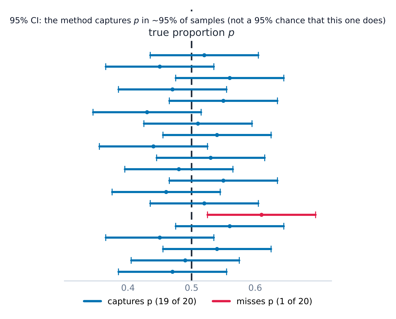
$z^{*}$ is the critical value for the confidence level 置信水平 (e.g. $1.96$ for 95%). Conditions: random sample, Large Counts ($n\hat p\ge 10$ and $n(1-\hat p)\ge 10$), and the 10% condition. Interpret it: "We are 95% confident the true proportion of... is between... and...". Interpret the level: "In 95% of samples, this method produces an interval that captures the true proportion."

Over many samples, about 95% of 95% confidence intervals capture the true proportion

Worked example. In a random sample of $200$ people, $120$ support a policy, so $\hat{p}=0.60$. A $95\%$ interval uses $z^*=1.96$:

We are $95\%$ confident the true proportion of supporters is between $53.2\%$ and $66.8\%$.

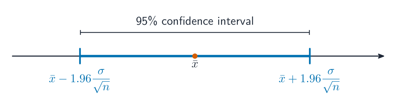
A 95% confidence interval reaches 1.96 standard errors each side of the estimate

Choosing the sample size. To keep the margin of error no larger than a target $m$, set $z^{*}\sqrt{\dfrac{\hat p(1-\hat p)}{n}}\le m$ and solve for $n$. When you have no estimate of $\hat p$, use $\hat p=0.5$: it makes $\hat p(1-\hat p)$ as large as possible, giving the safe (largest) required sample size. Always round the result up to the next whole person.

Worked example. How many people must you survey for a $95\%$ interval with margin of error at most $0.03$? Using $\hat p=0.5$ and $z^*=1.96$:

so you survey $1068$ people (always round up, since $1067$ would leave the margin a shade too big).

To judge a claimed value: if it lies inside the interval, the data are consistent with it; if it lies outside, the data give evidence against it. Base the conclusion on whether the plausible values include the claim, in context.

A significance test 显著性检验 weighs evidence against a claim. State a null hypothesis 原假设 $H_0$ and an alternative hypothesis 备择假设 $H_a$ about the parameter $p$:

Check the same conditions (random, Large Counts using $p_0$, 10%). The test statistic 检验统计量 counts standard errors from $p_0$:

Worked example. A company claims $90\%$ satisfaction ($p_0=0.90$); a sample of $100$ finds $84$ satisfied ($\hat{p}=0.84$). Test $H_0:p=0.90$ vs $H_a:p\neq0.90$ at $\alpha=0.05$:

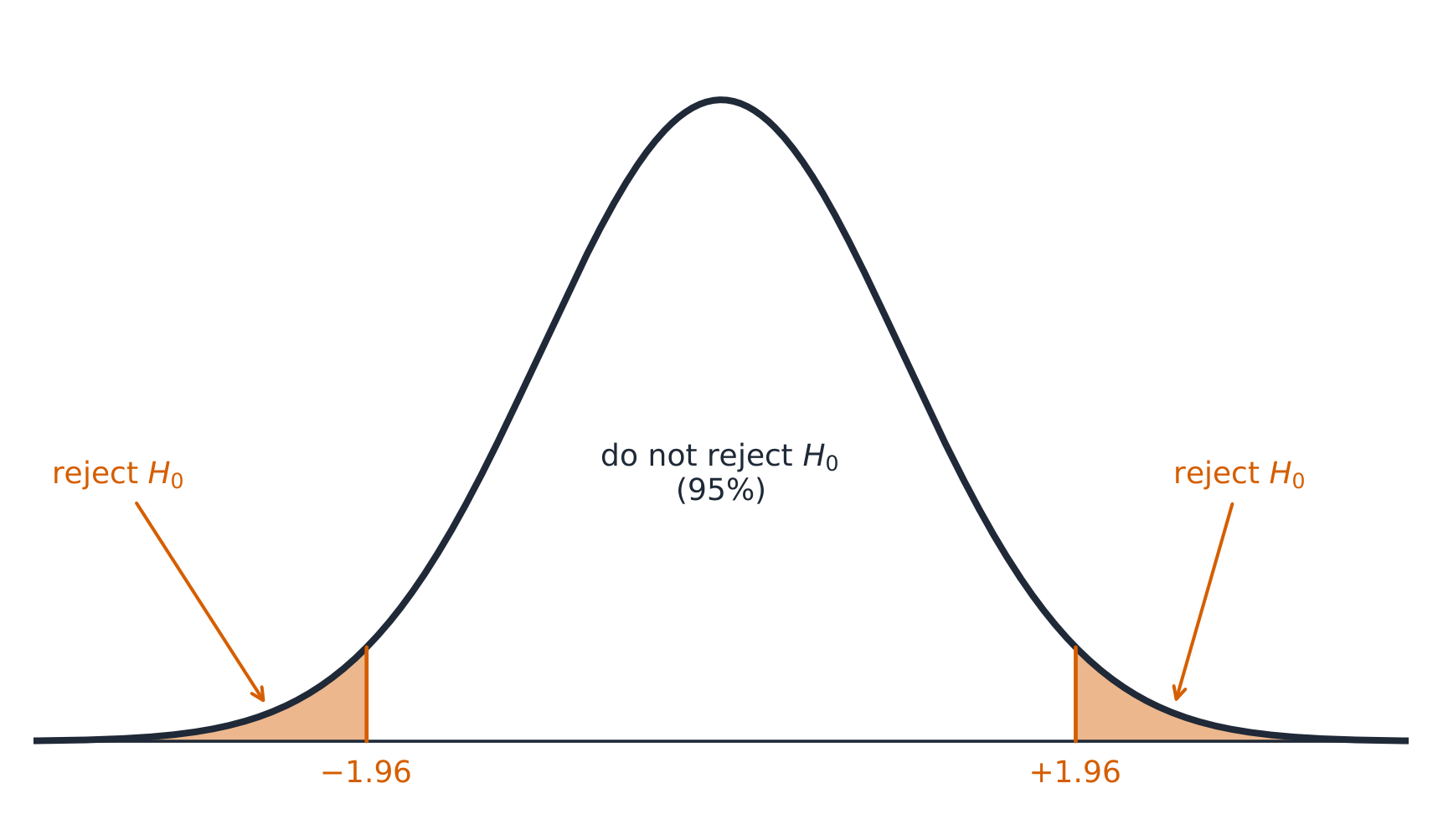
giving a two-tailed $p$-value of about $2(0.023)=0.046$. Since $0.046<0.05$, reject $H_0$ – there is evidence the true satisfaction rate differs from (is below) $90\%$.

A two-tailed 5% test rejects the null hypothesis in the shaded tails

The $p$-value P值 is the probability of getting a sample result as extreme or more extreme than the observed one, assuming $H_0$ is true. A small $p$-value means the data would be surprising if $H_0$ held – evidence against $H_0$. It is not the probability that $H_0$ is true.

Compare the $p$-value to the significance level 显著性水平 $\alpha$ (often $0.05$):

• $p\le\alpha$: reject $H_0$ – there is convincing evidence for $H_a$.
• $p>\alpha$: fail to reject $H_0$ – not enough evidence for $H_a$ (never "accept $H_0$").

Always write the conclusion in context, linking back to the claim.

• A Type I error 第一类错误: rejecting a true $H_0$ (a false alarm). Its probability is $\alpha$.
• A Type II error 第二类错误: failing to reject a false $H_0$ (a missed detection). Its probability is $\beta$.
• The power 检验效能 $=1-\beta$ is the chance of correctly detecting a real effect. Power rises with a larger sample, a larger effect, or a larger $\alpha$.

Describe each error and its consequence in the problem's context.

To compare two proportions, estimate $p_1-p_2$:

Conditions must hold in both samples, and the samples must be independent.

If the interval for $p_1-p_2$ contains $0$, the data are consistent with no difference; if it lies entirely above or below $0$, there is evidence of a difference (in that direction). State the direction and context.

Hypotheses compare the two proportions: $H_0: p_1=p_2$ versus $H_a: p_1\neq p_2$ (or $<,>$). Because $H_0$ says the proportions are equal, use a combined (pooled) 合并 sample proportion $\hat p_c=\dfrac{\text{total successes}}{\text{total sample size}}$ to estimate the common $p$.

The pooled two-proportion $z$ statistic:

Find the $p$-value from the normal model, compare to $\alpha$, and conclude in context – the same four-step logic as the one-proportion test.

• State the conditions (random, 10%, large counts $np,\,nq\ge10$) before any proportion inference.
• A confidence interval = estimate $\pm$ margin of error; "95% confident" refers to the method's long-run capture rate.
• For a test, write $H_0$ and $H_a$, compute the test statistic, find the p-value, and compare to $\alpha$.
• A small p-value is evidence against $H_0$; failing to reject does not prove $H_0$.
• Larger samples shrink the margin of error; a higher confidence level widens it.