| Enduring Understanding | Learning Objective | Essential Knowledge |
|---|---|---|
VAR-1 | VAR-1.A |
|
Tips
AP Statistics covers exploring data, sampling and experimental design, probability and random variables, sampling distributions, and inference — confidence intervals and significance tests. There is little algebra; the difficulty is saying the right thing about uncertainty.
Every inference answer has four parts: name the procedure, check the conditions, compute, and conclude in context with a link to the alternative hypothesis. The rubric grades all four, so a correct p-value alone scores poorly.
Language is graded. "We reject H₀" is not "we prove H₁"; a confidence interval is about the method's long-run behaviour, not the probability that a particular interval contains the parameter. These distinctions decide marks.
The notes work through all nine units with each inference procedure set out step by step. Released FRQs are in the library. Statistics gives marks for stating the conditions and interpreting in context, so every worked answer names the conditions before it runs the test.
-
1
Exploring One-Variable Data
Watch lesson1.1
Introducing Statistics: What Can We Learn from Data?
Syllabus
Source: College Board AP Course and Exam Description
Statistics 统计学 is the science of learning from data 数据 – numbers or labels collected from the real world. Data vary, so we describe patterns and account for the variation 变异 rather than expecting every value to match. A statistical question anticipates an answer based on data that vary.
Two distinctions run through the whole course. A parameter 参数 is a numerical summary of a whole population; a statistic 统计量 is a numerical summary of a sample - we use the statistic to estimate the parameter we cannot measure directly. And descriptive statistics 描述统计 only summarise the data set in hand, while inferential statistics 推断统计 use a sample to make and test claims about the larger population.
Vocabulary TrainEnglish Statistics/stəˈtɪstɪks/ data/ˈdeɪtə/ variation/ˌveərɪˈeɪʃn/ parameter/pəˈræmɪtə/ statistic/stəˈtɪstɪk/ descriptive statistics/dɪˈskrɪptɪv stəˈtɪstɪks/ inferential statistics/ɪnfəˈrenʃl stəˈtɪstɪks/ 1.2
The Language of Variation: Variables
Syllabus
Enduring Understanding Learning Objective Essential Knowledge VAR-1
Given that variation may be random or not, conclusions are uncertain.VAR-1.B
Identify variables in a set of data. [Skill 2.A]- VAR-1.B.1 A variable is a characteristic that changes from one individual to another.
VAR-1.C
Classify types of variables. [Skill 2.A]- VAR-1.C.1 A categorical variable takes on values that are category names or group labels.
- VAR-1.C.2 A quantitative variable is one that takes on numerical values for a measured or counted quantity.
- Illustrative examples for VAR-1.C:
- Categorical variables:
- Dominant hand
- Age group (young or old)
- Highest degree earned
- Quantitative variables:
- Age of a structure
- Height of a child
- Concentration of a sample
- Categorical variables:
- Illustrative examples for VAR-1.C:
Source: College Board AP Course and Exam Description
A variable 变量 is a characteristic that can differ between individuals. Two kinds:
- Categorical 分类 (qualitative): values are labels/groups (eye colour, brand).
- Quantitative 定量: values are numbers you can do arithmetic on (height, age). Quantitative variables are discrete (countable) or continuous (measured).
Choosing the right graph and summary depends on which kind you have.
ExploreCategorical or quantitative?
Every variable is either categorical (it labels each unit with a group) or quantitative (a measured number you can average). Which kind it is decides the graphs and summaries you are allowed to use.
Vocabulary TrainEnglish variable/ˈveərɪəbl/ Categorical/ˌkætɪˈɡɒrɪkl/ Quantitative/ˈkwɒntɪteɪtɪv/ 1.3
Representing a Categorical Variable with Tables
Syllabus
Enduring Understanding Learning Objective Essential Knowledge UNC-1
Graphical representations and statistics allow us to identify and represent key features of data.UNC-1.A
Represent categorical data using frequency or relative frequency tables. [Skill 2.B]- UNC-1.A.1 A frequency table gives the number of cases falling into each category. A relative frequency table gives the proportion of cases falling into each category.
UNC-1.B
Describe categorical data represented in frequency or relative tables. [Skill 2.A]- UNC-1.B.1 Percentages, relative frequencies, and rates all provide the same information as proportions.
- UNC-1.B.2 Counts and relative frequencies of categorical data reveal information that can be used to justify claims about the data in context.
Source: College Board AP Course and Exam Description
A frequency table 频数表 lists each category's count (frequency); a relative frequency 相对频率 table lists each category's proportion 比例 (count ÷ total). Relative frequencies let you compare groups of different sizes fairly.
Vocabulary TrainEnglish frequency table/ˈfriːkwənsi ˈteɪbl/ relative frequency/ˈrelətɪv ˈfriːkwənsi/ proportion/prəˈpɔːʃn/ 1.4
Representing a Categorical Variable with Graphs
Syllabus
Enduring Understanding Learning Objective Essential Knowledge UNC-1
Graphical representations and statistics allow us to identify and represent key features of data.UNC-1.C
Represent categorical data graphically. [Skill 2.B]- UNC-1.C.1 Bar charts (or bar graphs) are used to display frequencies (counts) or relative frequencies (proportions) for categorical data.
- UNC-1.C.2 The height or length of each bar in a bar graph corresponds to either the number or proportion of observations falling within each category.
- UNC-1.C.3 There are many additional ways to represent frequencies (counts) or relative frequencies (proportions) for categorical data.
UNC-1.D
Describe categorical data represented graphically. [Skill 2.A]- UNC-1.D.1 Graphical representations of a categorical variable reveal information that can be used to justify claims about the data in context.
UNC-1.E
Compare multiple sets of categorical data. [Skill 2.D]- UNC-1.E.1 Frequency tables, bar graphs, or other representations can be used to compare two or more data sets in terms of the same categorical variable.
Source: College Board AP Course and Exam Description
Bar charts 条形图 show the count or proportion of each category as separated bars; a pie chart shows each category's share of the whole. The bar heights (or slices) let you compare categories at a glance. Bars may be ordered by size or by a natural category order.
ExploreShow a categorical variable as a pie chart
A pie chart turns each category's share of the whole into a slice: a bigger share is a bigger slice, and every slice together makes 100%. It is a picture of a relative-frequency table.
Vocabulary TrainEnglish Bar charts/bɑː tʃɑːts/ 1.5
Representing a Quantitative Variable with Graphs
Syllabus
Enduring Understanding Learning Objective Essential Knowledge UNC-1
Graphical representations and statistics allow us to identify and represent key features of data.UNC-1.F
Classify types of quantitative variables. [Skill 2.A]- UNC-1.F.1 A discrete variable can take on a countable number of values. The number of values may be finite or countably infinite, as with the counting numbers.
- UNC-1.F.2 A continuous variable can take on infinitely many values, but those values cannot be counted. No matter how small the interval between two values of a continuous variable, it is always possible to determine another value between them.
- Illustrative examples for UNC-1.F:
- A discrete variable:
- Number of students in a class
- A continuous variable:
- Height of a child
- A discrete variable:
- Illustrative examples for UNC-1.F:
UNC-1.G
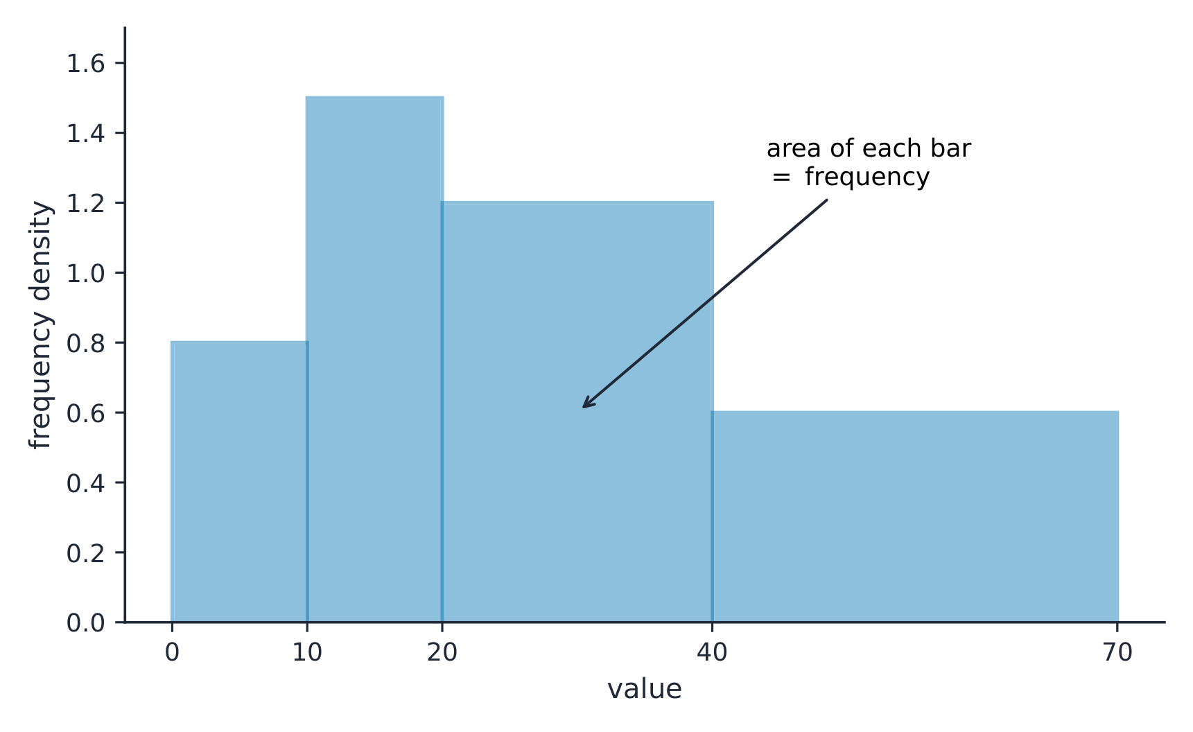
Represent quantitative data graphically. [Skill 2.B]- UNC-1.G.1 In a histogram, the height of each bar shows the number or proportion of observations that fall within the interval corresponding to that bar. Altering the interval widths can change the appearance of the histogram.
- UNC-1.G.2 In a stem and leaf plot, each data value is split into a "stem" (the first digit or digits) and a "leaf" (usually the last digit).
- UNC-1.G.3 A dotplot represents each observation by a dot, with the position on the horizontal axis corresponding to the data value of that observation, with nearly identical values stacked on top of each other.
- UNC-1.G.4 A cumulative graph represents the number or proportion of a data set less than or equal to a given number.
- UNC-1.G.5 There are many additional ways to graphically represent distributions of quantitative data.
Source: College Board AP Course and Exam Description
For numbers, use a dotplot 点图, stem-and-leaf plot 茎叶图, or histogram 直方图 (bars over value intervals called bins). These show the distribution 分布 – how the values spread out. A histogram's bin width changes the picture, so choose it to reveal the shape.
On a histogram with unequal class widths the bar area is the frequency ExploreExplore how bin width shapes a histogram
A histogram groups data into equal-width bins and draws a bar over each. Change the bins and notice how the same data can look jagged (too narrow) or smooth (too wide) — the shape is a choice.
Vocabulary TrainEnglish dotplot/ˈdɒtplɒt/ stem-and-leaf plot/stem ænd liːf plɒt/ histogram/ˈhɪstəɡræm/ distribution/ˌdɪstrɪˈbjuːʃn/ 1.6
Describing the Distribution of a Quantitative Variable
Syllabus
Enduring Understanding Learning Objective Essential Knowledge UNC-1
Graphical representations and statistics allow us to identify and represent key features of data.UNC-1.H
Describe the characteristics of quantitative data distributions. [Skill 2.A]- UNC-1.H.1 Descriptions of the distribution of quantitative data include shape, center, and variability (spread), as well as any unusual features such as outliers, gaps, clusters, or multiple peaks.
- UNC-1.H.2 Outliers for one-variable data are data points that are unusually small or large relative to the rest of the data.
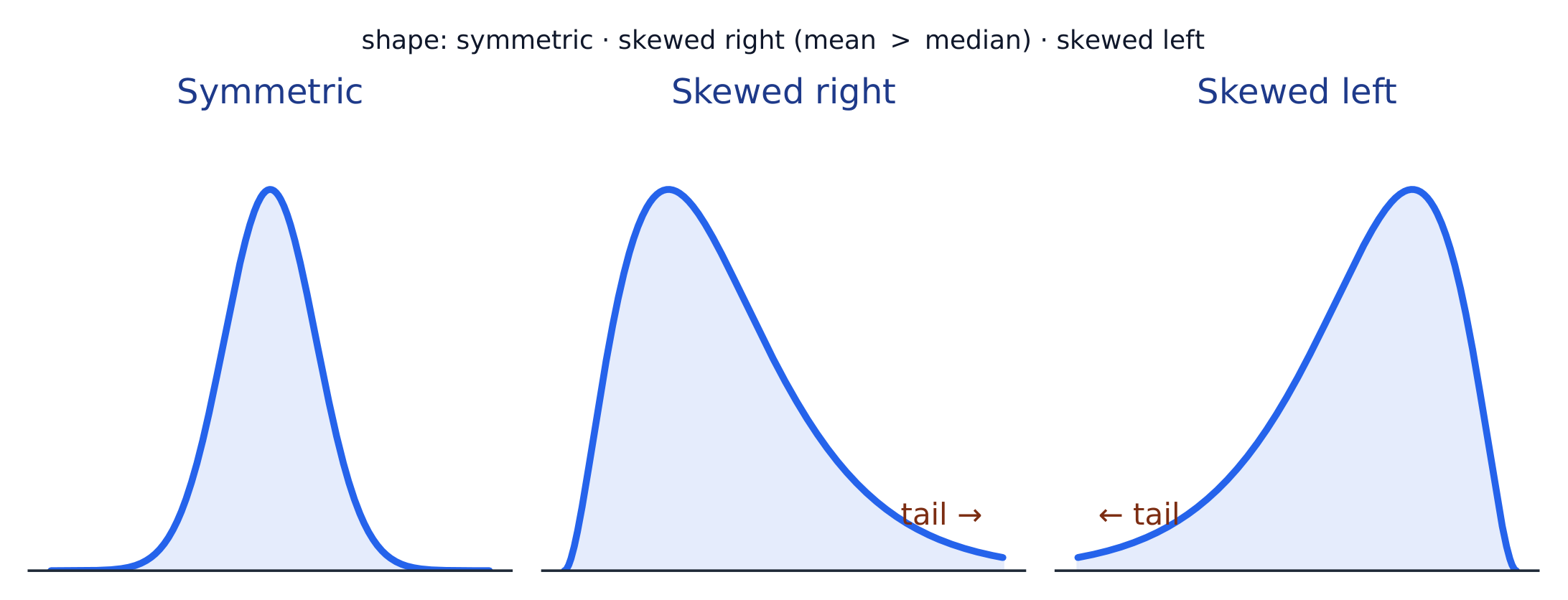
- UNC-1.H.3 A distribution is skewed to the right (positive skew) if the right tail is longer than the left. A distribution is skewed to the left (negative skew) if the left tail is longer than the right. A distribution is symmetric if the left half is the mirror image of the right half.
- UNC-1.H.4 Univariate graphs with one main peak are known as unimodal. Graphs with two prominent peaks are bimodal. A graph where each bar height is approximately the same (no prominent peaks) is approximately uniform.
- UNC-1.H.5 A gap is a region of a distribution between two data values where there are no observed data.
- UNC-1.H.6 Clusters are concentrations of data usually separated by gaps.
- UNC-1.H.7 Descriptive statistics does not attribute properties of a data set to a larger population, but may provide the basis for conjectures for subsequent testing.
Source: College Board AP Course and Exam Description
Describe four things (remember SOCS):
- Shape 形状: symmetric, or skewed 偏斜 left/right (a long tail on that side), and how many peaks - one main peak is unimodal 单峰, two prominent peaks bimodal 双峰, and roughly equal bars uniform 均匀.
- Outliers 离群值: unusual values far from the rest.
- Center: a typical value (mean or median).
- Spread: how much the values vary (range, IQR, standard deviation).
Always describe shape/center/spread in context, with units.
The shape of a distribution: symmetric, skewed right (long right tail), or skewed left Vocabulary TrainEnglish Shape/ʃeɪp/ skewed/skjuːd/ unimodal/ˌʌnɪˈmɒdl/ bimodal/baɪˈmɒdl/ uniform/ˈjuːnɪfɔːm/ Outliers/ˈaʊtlaɪəz/ 1.7
Summary Statistics for a Quantitative Variable
Syllabus
Enduring Understanding Learning Objective Essential Knowledge UNC-1
Graphical representations and statistics allow us to identify and represent key features of data.UNC-1.I
Calculate measures of center and position for quantitative data. [Skill 2.C]- UNC-1.I.1 A statistic is a numerical summary of sample data.
- UNC-1.I.2 The mean is the sum of all the data values divided by the number of values. For a sample, the mean is denoted by $x$-bar: $\bar{x} = \dfrac{1}{n}\sum_{i=1}^{n} x_i$, where $x_i$ represents the $i^{\text{th}}$ data point in the sample and $n$ represents the number of data values in the sample.
- UNC-1.I.3 The median of a data set is the middle value when data are ordered. When the number of data points is even, the median can take on any value between the two middle values. In AP Statistics, the most commonly used value for the median of a data set with an even number of values is the average of the two middle values.
- UNC-1.I.4 The first quartile, Q1, is the median of the half of the ordered data set from the minimum to the position of the median. The third quartile, Q3, is the median of the half of the ordered data set from the position of the median to the maximum. Q1 and Q3 form the boundaries for the middle 50% of values in an ordered data set.
- UNC-1.I.5 The $p^{\text{th}}$ percentile is interpreted as the value that has $p\%$ of the data less than or equal to it.
UNC-1.J
Calculate measures of variability for quantitative data. [Skill 2.C]- UNC-1.J.1 Three commonly used measures of variability (or spread) in a distribution are the range, interquartile range, and standard deviation.
- UNC-1.J.2 The range is defined as the difference between the maximum data value and the minimum data value. The interquartile range (IQR) is defined as the difference between the third and first quartiles: $Q3 - Q1$. Both the range and the interquartile range are possible ways of measuring variability of the distribution of a quantitative variable.
- UNC-1.J.3 Standard deviation is a way to measure variability of the distribution of a quantitative variable. For a sample, the standard deviation is denoted by $s$: $s_x = \sqrt{\dfrac{1}{n-1}\sum(x_i - \bar{x})^2}$. The square of the sample standard deviation, $s^2$, is called the sample variance.
- UNC-1.J.4 Changing units of measurement affects the values of the calculated statistics.
UNC-1.K
Explain the selection of a particular measure of center and/or variability for describing a set of quantitative data. [Skill 4.B]- UNC-1.K.1 There are many methods for determining outliers. Two methods frequently used in this course are:
- UNC-1.K.1.i An outlier is a value greater than $1.5 \times \text{IQR}$ above the third quartile or more than $1.5 \times \text{IQR}$ below the first quartile.
- UNC-1.K.1.ii An outlier is a value located 2 or more standard deviations above, or below, the mean.
- UNC-1.K.2 The mean, standard deviation, and range are considered nonresistant (or non-robust) because they are influenced by outliers. The median and IQR are considered resistant (or robust), because outliers do not greatly (if at all) affect their value.
Source: College Board AP Course and Exam Description
Standard deviation: spread about the mean - Center: the mean 均值 $\bar{x}=\dfrac{\sum x_i}{n}$ (average) and the median 中位数 (middle value). The median resists outliers; the mean is pulled toward a skew.
- Spread: the range, the interquartile range 四分位距 $\text{IQR}=Q_3-Q_1$ (middle 50%), and the standard deviation 标准差 $s_x=\sqrt{\dfrac{\sum(x_i-\bar{x})^2}{n-1}}$ (typical distance from the mean; its square is the variance 方差).
- The five-number summary 五数概括: min, $Q_1$, median, $Q_3$, max.
Use resistant measures (median, IQR) for skewed data; mean and standard deviation for roughly symmetric data.
The percentile 百分位数 of a value is the percent of the data at or below it – so the median is the 50th percentile and $Q_1$ the 25th. A cumulative relative frequency graph 累积相对频率图 makes percentiles easy to read: for each value it plots the proportion of the data at or below it, rising from 0 to 1. Go up from a value to the curve and across to its percentile, or reverse the steps to find the value at a given percentile (the same reading works from a cumulative-frequency table).
Worked example. For the data $4, 8, 6, 10, 7$: the mean is $\bar{x}=\dfrac{4+8+6+10+7}{5}=\dfrac{35}{5}=7$. Sorting to $4,6,7,8,10$, the median is the middle value, $7$. The mean and median agree here because the data are roughly symmetric.
Vocabulary TrainEnglish mean/miːn/ median/ˈmiːdiːən/ interquartile range/ˌɪntəˈkwɔːtaɪl reɪndʒ/ standard deviation/ˈstændəd ˌdiːvɪˈeɪʃn/ variance/ˈveərɪəns/ five-number summary/faɪv ˈnʌmbə ˈsʌməri/ percentile/pəˈsentaɪl/ cumulative relative frequency graph/ˈkjuːmjʊlətɪv ˈrelətɪv ˈfriːkwənsi ɡræf/ 1.8
Graphical Representations of Summary Statistics
Syllabus
Enduring Understanding Learning Objective Essential Knowledge UNC-1
Graphical representations and statistics allow us to identify and represent key features of data.UNC-1.L
Represent summary statistics for quantitative data graphically. [Skill 2.B]- UNC-1.L.1 Taken together, the minimum data value, the first quartile (Q1), the median, the third quartile (Q3), and the maximum data value make up the five-number summary.
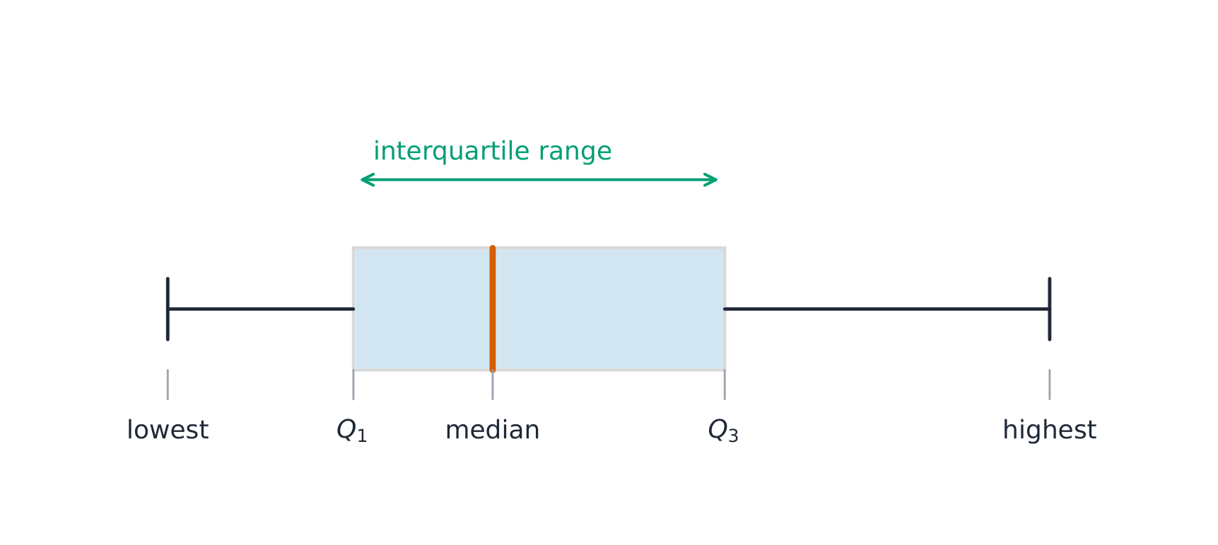
- UNC-1.L.2 A boxplot is a graphical representation of the five-number summary (minimum, first quartile, median, third quartile, maximum). The box represents the middle 50% of data, with a line at the median and the ends of the box corresponding to the quartiles. Lines ("whiskers") extend from the quartiles to the most extreme point that is not an outlier, and outliers are indicated by their own symbol beyond this.
UNC-1.M
Describe summary statistics of quantitative data represented graphically. [Skill 2.A]- UNC-1.M.1 Summary statistics of quantitative data, or of sets of quantitative data, can be used to justify claims about the data in context.
- UNC-1.M.2 If a distribution is relatively symmetric, then the mean and median are relatively close to one another. If a distribution is skewed right, then the mean is usually to the right of the median. If the distribution is skewed left, then the mean is usually to the left of the median.
Source: College Board AP Course and Exam Description
A boxplot 箱线图 draws the five-number summary: a box from $Q_1$ to $Q_3$ with the median inside, and whiskers to the most extreme non-outlier values. A point is an outlier if it lies more than $1.5\times\text{IQR}$ beyond a quartile – a rule you may be asked to apply. Boxplots are ideal for comparing several groups side by side.
Worked example. A dataset has $Q_1=20$ and $Q_3=32$, so $\text{IQR}=12$. The outlier fences are $Q_1-1.5(12)=2$ and $Q_3+1.5(12)=50$. Any value below $2$ or above $50$ is flagged as an outlier.
A box-and-whisker plot shows the quartiles and the range 
A boxplot draws the five-number summary; the box spans the IQR ExploreExplore the five-number summary as a boxplot
Drag $Q_1$, the median, and $Q_3$ to see the box (its length is the IQR) and how the median's position inside the box reveals skew — a median close to $Q_1$ signals a right-skewed distribution.
Vocabulary TrainEnglish boxplot/ˈbɒksplɒt/ 1.9
Comparing Distributions of a Quantitative Variable
Syllabus
Enduring Understanding Learning Objective Essential Knowledge UNC-1
Graphical representations and statistics allow us to identify and represent key features of data.UNC-1.N
Compare graphical representations for multiple sets of quantitative data. [Skill 2.D]- UNC-1.N.1 Any of the graphical representations, e.g., histograms, side-by-side boxplots, etc., can be used to compare two or more independent samples on center, variability, clusters, gaps, outliers, and other features.
UNC-1.O
Compare summary statistics for multiple sets of quantitative data. [Skill 2.D]- UNC-1.O.1 Any of the numerical summaries (e.g., mean, standard deviation, relative frequency, etc.) can be used to compare two or more independent samples.
Source: College Board AP Course and Exam Description
To compare two or more groups, compare shape, center, and spread, and mention outliers – always with comparative words ("Group A has a higher median than Group B") and in context. Do not just describe each group separately; make the comparison explicit.
ExploreCompare distributions with box plots
A box plot draws the five-number summary. Placing two box plots on the same scale compares their centre (median), spread (IQR = box width) and skew at a glance — the fair way to compare groups.
1.10
The Normal Distribution
Syllabus
Enduring Understanding Learning Objective Essential Knowledge VAR-2
The normal distribution can be used to represent some population distributions.VAR-2.A
Compare a data distribution to the normal distribution model. [Skill 2.D]- VAR-2.A.1 A parameter is a numerical summary of a population.
- VAR-2.A.2 Some sets of data may be described as approximately normally distributed. A normal curve is mound-shaped and symmetric. The parameters of a normal distribution are the population mean, $\mu$, and the population standard deviation, $\sigma$.
- VAR-2.A.3 For a normal distribution, approximately 68% of the observations are within 1 standard deviation of the mean, approximately 95% of observations are within 2 standard deviations of the mean, and approximately 99.7% of observations are within 3 standard deviations of the mean. This is called the empirical rule.
- VAR-2.A.4 Many variables can be modeled by a normal distribution.
- Illustrative examples for VAR-2.A:
- Variables that can be modeled by a normal distribution:
- Body temperature
- Weight of a loaf of bread
- Variables that can be modeled by a normal distribution:
- Illustrative examples for VAR-2.A:
VAR-2.B
Determine proportions and percentiles from a normal distribution. [Skill 3.A]- VAR-2.B.1 A standardized score for a particular data value is calculated as (data value − mean)/(standard deviation), and measures the number of standard deviations a data value falls above or below the mean.
- VAR-2.B.2 One example of a standardized score is a $z$-score, which is calculated as $z\text{-score} = \left(\dfrac{x_i - \mu}{\sigma}\right)$. A $z$-score measures how many standard deviations a data value is from the mean.
- VAR-2.B.3 Technology, such as a calculator, a standard normal table, or computer-generated output, can be used to find the proportion of data values located on a given interval of a normally distributed random variable.
- VAR-2.B.4 Given the area of a region under the graph of the normal distribution curve, it is possible to use technology, such as a calculator, a standard normal table, or computer-generated output, to estimate parameters for some populations.
VAR-2.C
Compare measures of relative position in data sets. [Skill 2.D]- VAR-2.C.1 Percentiles and $z$-scores may be used to compare relative positions of points within a data set or between data sets.
Source: College Board AP Course and Exam Description
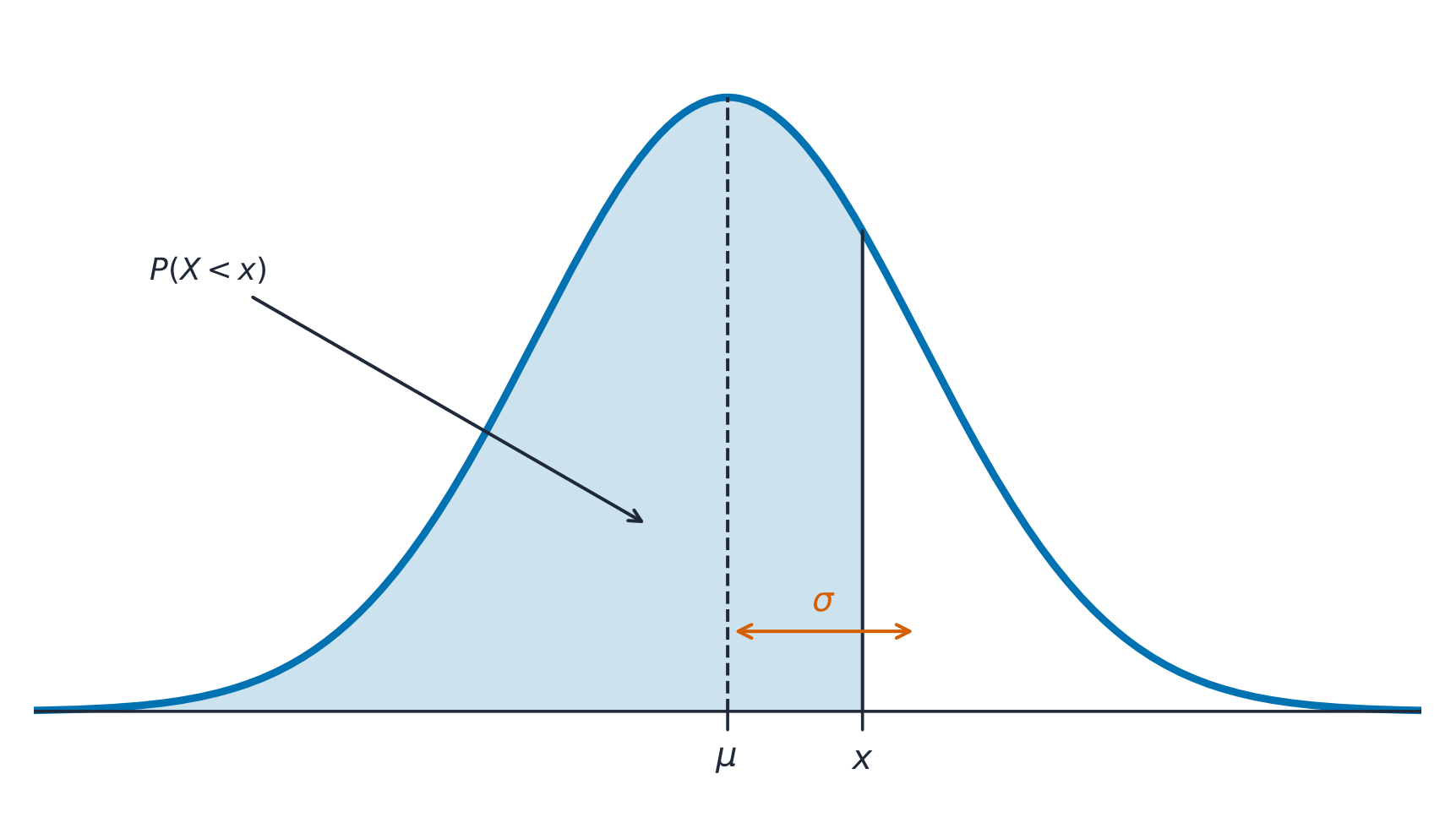
A normal distribution 正态分布 is a symmetric, bell-shaped model described by its mean $\mu$ and standard deviation $\sigma$. The empirical rule 经验法则 (68–95–99.7): about 68% of values lie within $1\sigma$ of the mean, 95% within $2\sigma$, and 99.7% within $3\sigma$.
The normal curve: a probability is the area under it, centred on the mean A $z$-score 标准分数 measures how many standard deviations a value is from the mean:
$$z=\frac{x-\mu}{\sigma}.$$Convert to a $z$-score, then use the normal table or technology to find the proportion (area) below, above, or between values – and reverse the process to find a value from a given percentile.Worked example. Test scores are normal with $\mu=500$ and $\sigma=100$. A score of $700$ has $z=\dfrac{700-500}{100}=2$. By the empirical rule, $95\%$ of scores lie within $2\sigma$, so $2.5\%$ lie above $700$ – meaning a $700$ is at about the $97.5$th percentile.
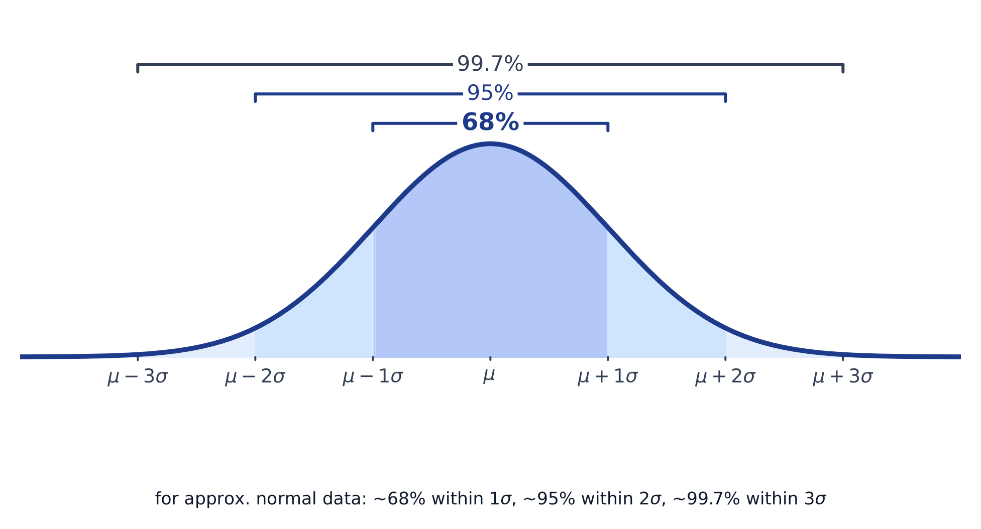
The normal curve and the 68-95-99.7 empirical rule ExploreExplore area under the normal curve
The proportion of data below a value equals the area under the curve to its left. Shade a tail or a central band to see the 68–95–99.7 empirical rule and read a $z$-score as an area.
Vocabulary TrainEnglish normal distribution/ˈnɔːml ˌdɪstrɪˈbjuːʃn/ empirical rule/emˈpɪrɪkl ruːl/ $z$-score/ˈzed skɔː/ 1.10
Exam tips
- Describe a distribution by shape, center, spread, and outliers (SOCS) — always in context.
- The mean is pulled by outliers; the median resists them, so prefer the median for skewed data.
- For a normal distribution use the 68–95–99.7 rule and z-scores $z=\tfrac{x-\mu}{\sigma}$.
- Compare distributions with side-by-side boxplots and comment on center, spread, and shape.
- Standard deviation measures a typical distance from the mean; the IQR pairs with the median.
-
2
Exploring Two-Variable Data
Watch lesson2.1
Are Two Variables Related?
Syllabus
Enduring Understanding Learning Objective Essential Knowledge VAR-1
Given that variation may be random or not, conclusions are uncertain.VAR-1.D
Identify questions to be answered about possible relationships in data. [Skill 1.A]- VAR-1.D.1 Apparent patterns and associations in data may be random or not.
Source: College Board AP Course and Exam Description
Two-variable data let us ask whether two characteristics are associated 关联 – whether knowing one tells you something about the other. An explanatory variable 解释变量 (the "input") may help predict a response variable 响应变量 (the "output"). Association is not the same as causation.
Vocabulary TrainEnglish associated/əˈsəʊsɪeɪtɪd/ explanatory variable/ekˈsplænətəri ˈveərɪəbl/ response variable/rɪˈspɒns ˈveərɪəbl/ 2.2
Two Categorical Variables
Syllabus
Enduring Understanding Learning Objective Essential Knowledge UNC-1
Graphical representations and statistics allow us to identify and represent key features of data.UNC-1.P
Compare numerical and graphical representations for two categorical variables. [Skill 2.D]- UNC-1.P.1 Side-by-side bar graphs, segmented bar graphs, and mosaic plots are examples of bar graphs for one categorical variable, broken down by categories of another categorical variable.
- UNC-1.P.2 Graphical representations of two categorical variables can be used to compare distributions and/or determine if variables are associated.
- UNC-1.P.3 A two-way table, also called a contingency table, is used to summarize two categorical variables. The entries in the cells can be frequency counts or relative frequencies.
- UNC-1.P.4 A joint relative frequency is a cell frequency divided by the total for the entire table.
Source: College Board AP Course and Exam Description
A two-way table 双向表 (contingency table) counts individuals by two categorical variables at once. A marginal distribution 边缘分布 is a row or column total written as a fraction of the grand total (the totals themselves are just counts). Comparing the inside cells shows whether the variables are related.
Vocabulary TrainEnglish two-way table/tuː weɪ ˈteɪbl/ marginal distributions/ˈmɑːdʒɪnl ˌdɪstrɪˈbjuːʃnz/ 2.3
Comparing Groups with Conditional Distributions
Syllabus
Enduring Understanding Learning Objective Essential Knowledge UNC-1
Graphical representations and statistics allow us to identify and represent key features of data.UNC-1.Q
Calculate statistics for two categorical variables. [Skill 2.C]- UNC-1.Q.1 The marginal relative frequencies are the row and column totals in a two-way table divided by the total for the entire table.
- UNC-1.Q.2 A conditional relative frequency is a relative frequency for a specific part of the contingency table (e.g., cell frequencies in a row divided by the total for that row).
UNC-1.R
Compare statistics for two categorical variables. [Skill 2.D]- UNC-1.R.1 Summary statistics for two categorical variables can be used to compare distributions and/or determine if variables are associated.
Source: College Board AP Course and Exam Description
A conditional distribution 条件分布 is the distribution of one variable within a fixed category of the other (found by dividing each cell by its row or column total). If the conditional distributions differ across groups, the two variables are associated; if they are the same, there is no association. Segmented bar charts 分段条形图 or mosaic plots display them.
Vocabulary TrainEnglish conditional distribution/kənˈdɪʃənl ˌdɪstrɪˈbjuːʃn/ Segmented bar charts/seɡˈmentɪd bɑː tʃɑːts/ 2.4
Scatterplots for Two Quantitative Variables
Syllabus
Enduring Understanding Learning Objective Essential Knowledge UNC-1
Graphical representations and statistics allow us to identify and represent key features of data.UNC-1.S
Represent bivariate quantitative data using scatterplots. [Skill 2.B]- UNC-1.S.1 A bivariate quantitative data set consists of observations of two different quantitative variables made on individuals in a sample or population.
- UNC-1.S.2 A scatterplot shows two numeric values for each observation, one corresponding to the value on the $x$-axis and one corresponding to the value on the $y$-axis.
- UNC-1.S.3 An explanatory variable is a variable whose values are used to explain or predict corresponding values for the response variable.
DAT-1
Regression models may allow us to predict responses to changes in an explanatory variable.DAT-1.A
Describe the characteristics of a scatter plot. [Skill 2.A]- DAT-1.A.1 A description of a scatter plot includes form, direction, strength, and unusual features.
- DAT-1.A.2 The direction of the association shown in a scatterplot, if any, can be described as positive or negative.
- DAT-1.A.3 A positive association means that as values of one variable increase, the values of the other variable tend to increase. A negative association means that as values of one variable increase, values of the other variable tend to decrease.
- DAT-1.A.4 The form of the association shown in a scatterplot, if any, can be described as linear or non-linear to varying degrees.
- DAT-1.A.5 The strength of the association is how closely the individual points follow a specific pattern, e.g., linear, and can be shown in a scatterplot. Strength can be described as strong, moderate, or weak.
- DAT-1.A.6 Unusual features of a scatter plot include clusters of points or points with relatively large discrepancies between the value of the response variable and a predicted value for the response variable.
Source: College Board AP Course and Exam Description
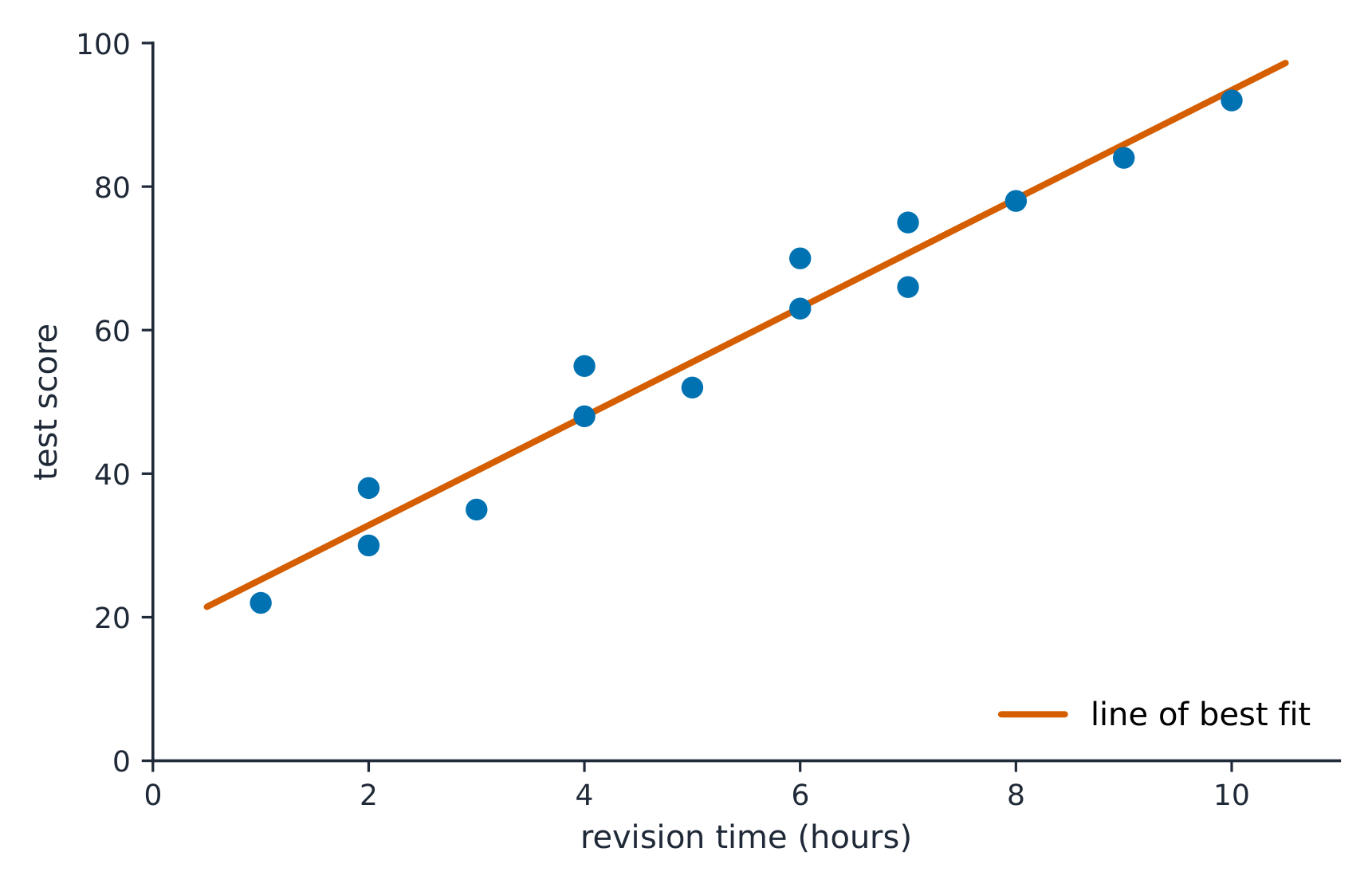
A scatterplot 散点图 plots each individual as a point, explanatory variable on the $x$-axis and response on the $y$-axis. Describe it with DUFS: Direction (positive/negative), Unusual features (outliers, clusters), Form (linear or curved), and Strength (how tightly the points follow the pattern) – always in context.
A line of best fit runs through the middle of the scattered points Vocabulary TrainEnglish scatterplot/ˈskætəplɒt/ 2.5
Correlation
Syllabus
Enduring Understanding Learning Objective Essential Knowledge DAT-1
Regression models may allow us to predict responses to changes in an explanatory variable.DAT-1.B
Determine the correlation for a linear relationship. [Skill 2.C]- DAT-1.B.1 The correlation, $r$, gives the direction and quantifies the strength of the linear association between two quantitative variables.
- DAT-1.B.2 The correlation coefficient can be calculated by: $r = \dfrac{1}{n-1} \sum \left( \dfrac{x_i - \bar{x}}{s_x} \right) \left( \dfrac{y_i - \bar{y}}{s_y} \right)$. However, the most common way to determine $r$ is by using technology.
- DAT-1.B.3 A correlation coefficient close to 1 or $-1$ does not necessarily mean that a linear model is appropriate.
DAT-1.C
Interpret the correlation for a linear relationship. [Skill 4.B]- DAT-1.C.1 The correlation, $r$, is unit-free, and always between $-1$ and 1, inclusive. A value of $r = 0$ indicates that there is no linear association. A value of $r = 1$ or $r = -1$ indicates that there is a perfect linear association.
- DAT-1.C.2 A perceived or real relationship between two variables does not mean that changes in one variable cause changes in the other. That is, correlation does not necessarily imply causation.
Source: College Board AP Course and Exam Description
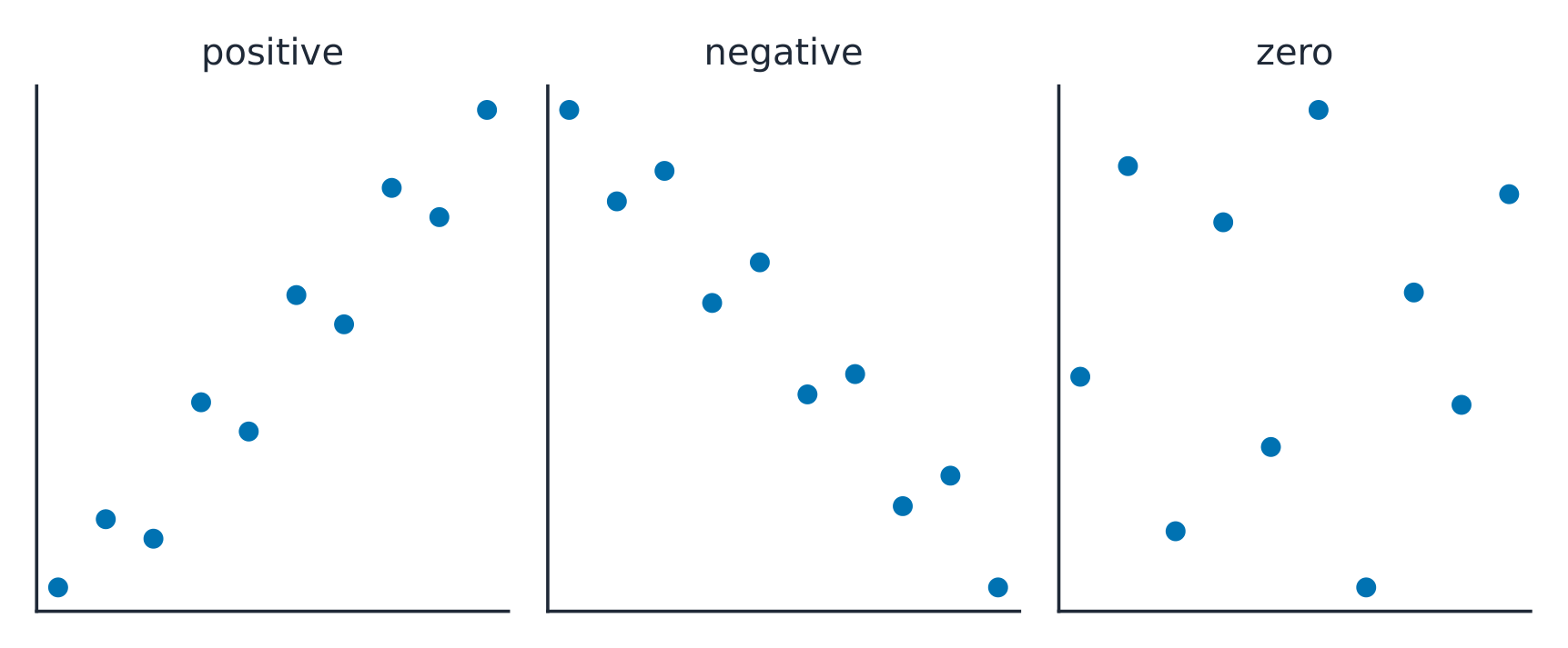
What r actually measures The correlation coefficient 相关系数 $r$ measures the strength and direction of a linear relationship. It runs from $-1$ to $1$: near $\pm 1$ is strong linear, near $0$ is weak linear. $r$ has no units and does not change if you swap the variables. Warnings: $r$ only measures linear strength, it is not resistant to outliers, and a strong $r$ does not prove causation.
Positive correlation rises together; negative correlation moves in opposite directions ExploreStrength of a linear relationship
Correlation $r$ runs from $-1$ to $1$: near $\pm1$ the points hug a line, near 0 they scatter. Change it and watch the cloud tighten or spread.
Vocabulary TrainEnglish correlation coefficient/ˌkɒrɪˈleɪʃn ˌkəʊɪˈfɪʃənt/ 2.6
Linear Regression Models
Syllabus
Enduring Understanding Learning Objective Essential Knowledge DAT-1
Regression models may allow us to predict responses to changes in an explanatory variable.DAT-1.D
Calculate a predicted response value using a linear regression model. [Skill 2.C]- DAT-1.D.1 A simple linear regression model is an equation that uses an explanatory variable, $x$, to predict the response variable, $y$.
- DAT-1.D.2 The predicted response value, denoted by $\hat{y}$, is calculated as $\hat{y} = a + bx$, where $a$ is the $y$-intercept and $b$ is the slope of the regression line, and $x$ is the value of the explanatory variable.
- DAT-1.D.3 Extrapolation is predicting a response value using a value for the explanatory variable that is beyond the interval of $x$-values used to determine the regression line. The predicted value is less reliable as an estimate the further we extrapolate.
Source: College Board AP Course and Exam Description
The least-squares regression line 最小二乘回归线 predicts the response: $\hat{y}=a+bx$, where $\hat{y}$ is the predicted response. The slope 斜率 $b$ is the predicted change in $y$ per one-unit increase in $x$; the $y$-intercept 截距 $a$ is the predicted $y$ when $x=0$. Interpret both in context and with units – a graded skill. Avoid extrapolation 外推 (predicting far outside the data).
Worked example. A study of hours studied ($x$) and test score ($y$) gives $\hat{y}=20+3x$. The slope means each extra hour of study is associated with a predicted $3$-point increase. A student who studies $5$ hours is predicted to score $\hat{y}=20+3(5)=35$.
ExploreFit a least-squares line
A regression line is the best straight-line fit, minimising the squared vertical distances. Its slope predicts how $y$ changes per unit of $x$.
Vocabulary TrainEnglish least-squares regression line/liːst skweəz rɪˈɡreʃn laɪn/ slope/sləʊp/ y-intercept/waɪ ˌɪntəˈsept/ extrapolation/ekˈstræpəleɪʃn/ 2.7
Residuals
Syllabus
Enduring Understanding Learning Objective Essential Knowledge DAT-1
Regression models may allow us to predict responses to changes in an explanatory variable.DAT-1.E
Represent differences between measured and predicted responses using residual plots. [Skill 2.B]- DAT-1.E.1 The residual is the difference between the actual value and the predicted value: $\text{residual} = y - \hat{y}$.
- DAT-1.E.2 A residual plot is a plot of residuals versus explanatory variable values or predicted response values.
DAT-1.F
Describe the form of association of bivariate data using residual plots. [Skill 2.A]- DAT-1.F.1 Apparent randomness in a residual plot for a linear model is evidence of a linear form to the association between the variables.
- DAT-1.F.2 Residual plots can be used to investigate the appropriateness of a selected model.
Source: College Board AP Course and Exam Description
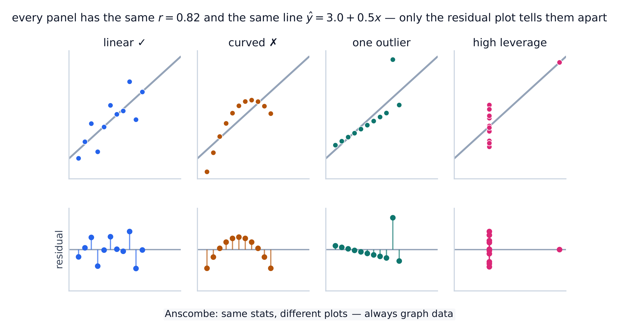
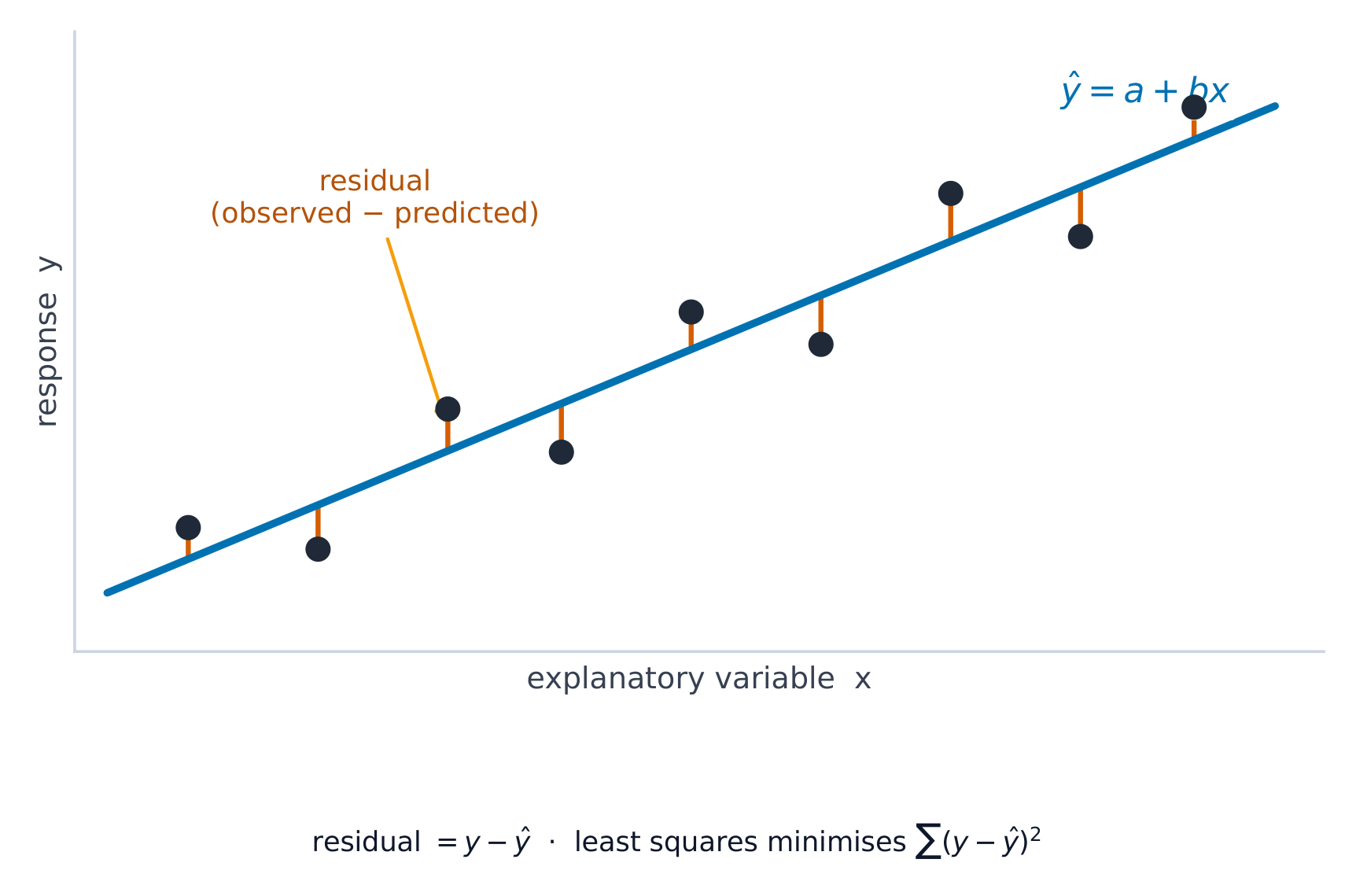
Least-squares regression A residual 残差 is actual minus predicted, $y-\hat{y}$: how far a point sits above (+) or below (−) the line. A residual plot 残差图 graphs residuals against $x$. If it shows no pattern (random scatter), a linear model is appropriate; a curved or fanning pattern means the linear model is a poor fit.
Worked example. Continuing the study above, a student who studied $5$ hours actually scored $40$. The residual is $y-\hat{y}=40-35=+5$: the line under-predicted by $5$ points, so this point sits above the line.
A caution about $r$ and the line: all four datasets have the same $r=0.82$ and the same $\hat{y}=3.0+0.5x$, yet only the first is genuinely linear. The scatterplots barely differ — the residual plot below each is what exposes the curve, the outlier, and the high-leverage point. Vocabulary TrainEnglish residual/rɪˈsɪdʒuːəl/ residual plot/rɪˈsɪdʒuːəl plɒt/ 2.8
Least-Squares Regression and Its Fit
Syllabus
Enduring Understanding Learning Objective Essential Knowledge DAT-1
Regression models may allow us to predict responses to changes in an explanatory variable.DAT-1.G
Estimate parameters for the least-squares regression line model. [Skill 2.C]- DAT-1.G.1 The least-squares regression model minimizes the sum of the squares of the residuals and contains the point $(\bar{x}, \bar{y})$.
- DAT-1.G.2 The slope, $b$, of the regression line can be calculated as $b = r \left( \dfrac{s_y}{s_x} \right)$ where $r$ is the correlation between $x$ and $y$, $s_y$ is the sample standard deviation of the response variable, $y$, and $s_x$ is the sample standard deviation of the explanatory variable, $x$.
- DAT-1.G.3 Sometimes, the $y$-intercept of the line does not have a logical interpretation in context.
- DAT-1.G.4 In simple linear regression, $r^2$ is the square of the correlation, $r$. It is also called the coefficient of determination. $r^2$ is the proportion of variation in the response variable that is explained by the explanatory variable in the model.
DAT-1.H
Interpret coefficients for the least-squares regression line model. [Skill 4.B]- DAT-1.H.1 The coefficients of the least-squares regression model are the estimated slope and $y$-intercept.
- DAT-1.H.2 The slope is the amount that the predicted $y$-value changes for every unit increase in $x$.
- DAT-1.H.3 The $y$-intercept value is the predicted value of the response variable when the explanatory variable is equal to $0$. The formula for the $y$-intercept, $a$, is $a = \bar{y} - b\bar{x}$.
Source: College Board AP Course and Exam Description
The least-squares line minimizes the sum of squared residuals The line minimizes the sum of squared residuals. Its fit is measured by:
- $s$, the standard deviation of the residuals – the typical prediction error, in the response's units.
- $r^2$, the coefficient of determination 决定系数 – the proportion of the variation in $y$ that the linear model explains (a value between $0$ and $1$; multiply by $100$ to state it as a percent). Report it in context: "$r^2 = 0.81$ means 81% of the variation in $y$ is explained by the linear relationship with $x$."
Vocabulary TrainEnglish coefficient of determination/ˌkəʊɪˈfɪʃənt ɒv dɪˌtɜːmɪˈneɪʃn/ 2.9
Departures from Linearity
Syllabus
Enduring Understanding Learning Objective Essential Knowledge DAT-1
Regression models may allow us to predict responses to changes in an explanatory variable.DAT-1.I
Identify influential points in regression. [Skill 2.A]- DAT-1.I.1 An outlier in regression is a point that does not follow the general trend shown in the rest of the data and has a large residual when the Least Squares Regression Line (LSRL) is calculated.
- DAT-1.I.2 A high-leverage point in regression has a substantially larger or smaller $x$-value than the other observations have.
- DAT-1.I.3 An influential point in regression is any point that, if removed, changes the relationship substantially. Examples include much different slope, $y$-intercept, and/or correlation. Outliers and high leverage points are often influential.
DAT-1.J
Calculate a predicted response using a least-squares regression line for a transformed data set. [Skill 2.C]- DAT-1.J.1 Transformations of variables, such as evaluating the natural logarithm of each value of the response variable or squaring each value of the explanatory variable, can be used to create transformed data sets, which may be more linear in form than the untransformed data.
- DAT-1.J.2 Increased randomness in residual plots after transformation of data and/or movement of $r^2$ to a value closer to 1 offers evidence that the least-squares regression line for the transformed data is a more appropriate model to use to predict responses to the explanatory variable than the regression line for the untransformed data.
Source: College Board AP Course and Exam Description
Some points strongly affect the line. A high-leverage 高杠杆 point has an extreme $x$-value; an influential 有影响的 point noticeably changes the slope or $r$ when removed; an outlier here is a point with a large residual. When the pattern is curved, transform a variable (e.g. take a log) to straighten it, then fit a line to the transformed data.
Vocabulary TrainEnglish high-leverage/haɪ ˈliːvərɪdʒ/ influential/ˌɪnfluːˈenʃl/ 2.9
Exam tips
- On a scatterplot describe direction, form, strength, and outliers; $r$ ranges $-1$ to $1$.
- Correlation is not causation — a lurking variable can drive both.
- Interpret the slope of the least-squares line in context ("per one unit of $x$, predicted $y$ changes by $b$").
- Check a residual plot: no pattern means a line fits; a curve means it does not. Avoid extrapolation.
- $r^2$ is the fraction of variation in $y$ explained by the model.
-
3
Collecting Data
Watch lesson3.1
Can We Trust the Data We Collected?
Syllabus
Enduring Understanding Learning Objective Essential Knowledge VAR-1
Given that variation may be random or not, conclusions are uncertain.VAR-1.E
Identify questions to be answered about data collection methods. [Skill 1.A]- VAR-1.E.1 Methods for data collection that do not rely on chance result in untrustworthy conclusions.
Source: College Board AP Course and Exam Description
A conclusion is only as good as the data behind it. How data are collected decides what you may conclude – whether you can generalize to a population 总体, and whether you can claim cause and effect. Poorly collected data can be worse than none.
Vocabulary TrainEnglish population/ˌpɒpjʊˈleɪʃn/ 3.2
Observational Studies and Experiments
Syllabus
Enduring Understanding Learning Objective Essential Knowledge DAT-2
The way we collect data influences what we can and cannot say about a population.DAT-2.A
Identify the type of a study. [Skill 1.C]- DAT-2.A.1 A population consists of all items or subjects of interest.
- DAT-2.A.2 A sample selected for study is a subset of the population.
- DAT-2.A.3 In an observational study, treatments are not imposed. Investigators examine data for a sample of individuals (retrospective) or follow a sample of individuals into the future collecting data (prospective) in order to investigate a topic of interest about the population. A sample survey is a type of observational study that collects data from a sample in an attempt to learn about the population from which the sample was taken.
- DAT-2.A.4 In an experiment, different conditions (treatments) are assigned to experimental units (participants or subjects).
DAT-2.B
Identify appropriate generalizations and determinations based on observational studies. [Skill 4.A]- DAT-2.B.1 It is only appropriate to make generalizations about a population based on samples that are randomly selected or otherwise representative of that population.
- DAT-2.B.2 A sample is only generalizable to the population from which the sample was selected.
- DAT-2.B.3 It is not possible to determine causal relationships between variables using data collected in an observational study.
Source: College Board AP Course and Exam Description
- In an observational study 观察性研究 you measure individuals without trying to influence them. It can show association, but not causation, because lurking variables may explain the link.
- In an experiment 实验 you deliberately impose a treatment 处理 and compare responses. A well-designed experiment can establish cause and effect.
ExploreObservational study or experiment?
In an experiment the researcher imposes a treatment (and can show cause); an observational study only records what already happens (and can show association, not cause).
Vocabulary TrainEnglish observational study/ɒbzəˈveɪʃənl ˈstʌdi/ experiment/ekˈsperɪmənt/ treatment/ˈtriːtmənt/ 3.3
Random Sampling
Syllabus
Enduring Understanding Learning Objective Essential Knowledge DAT-2
The way we collect data influences what we can and cannot say about a population.DAT-2.C
Identify a sampling method, given a description of a study. [Skill 1.C]- DAT-2.C.1 When an item from a population can be selected only once, this is called sampling without replacement. When an item from the population can be selected more than once, this is called sampling with replacement.
- DAT-2.C.2 A simple random sample (SRS) is a sample in which every group of a given size has an equal chance of being chosen. This method is the basis for many types of sampling mechanisms. A few examples of mechanisms used to obtain SRSs include numbering individuals and using a random number generator to select which ones to include in the sample, ignoring repeats, using a table of random numbers, or drawing a card from a deck without replacement.
- DAT-2.C.3 A stratified random sample involves the division of a population into separate groups, called strata, based on shared attributes or characteristics (homogeneous grouping). Within each stratum a simple random sample is selected, and the selected units are combined to form the sample.
- DAT-2.C.4 A cluster sample involves the division of a population into smaller groups, called clusters. Ideally, there is heterogeneity within each cluster, and clusters are similar to one another in their composition. A simple random sample of clusters is selected from the population to form the sample of clusters. Data are collected from all observations in the selected clusters.
- DAT-2.C.5 A systematic random sample is a method in which sample members from a population are selected according to a random starting point and a fixed, periodic interval.
- DAT-2.C.6 A census selects all items/subjects in a population.
DAT-2.D
Explain why a particular sampling method is or is not appropriate for a given situation. [Skill 1.C]- DAT-2.D.1 There are advantages and disadvantages for each sampling method depending upon the question that is to be answered and the population from which the sample will be drawn.
Source: College Board AP Course and Exam Description
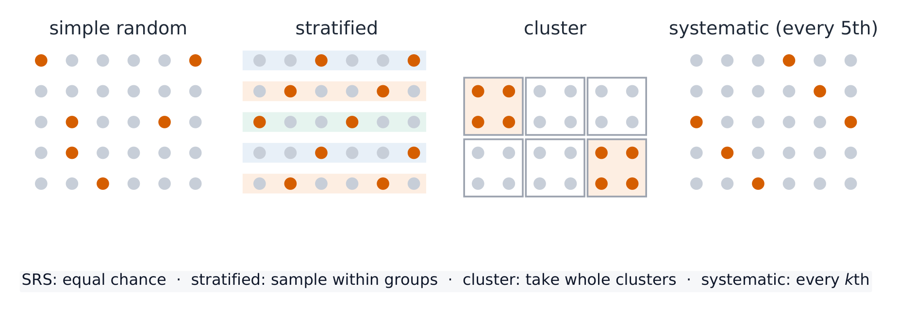
To learn about a population you take a sample 样本. Random sampling 随机抽样 protects against selection bias 偏差 and lets you generalize (it cannot fix undercoverage, nonresponse, or response bias — see below). Common designs:
- Simple random sample (SRS) 简单随机样本: every group of the chosen size is equally likely.
- Stratified 分层: split the population into similar strata, then sample within each.
- Cluster 整群: split into clusters, randomly choose whole clusters.
- Systematic 系统: pick every $k$th individual from a random start.
Four random sampling designs: who gets selected, and how A convenience sample 方便样本 or voluntary response sample is not random and is biased.
Worked example. To survey a school, an administrator lists all students by grade and randomly selects $20$ from each grade. This is a stratified sample – the grades are the strata – which guarantees every grade is represented, unlike an SRS that might by chance draw few from one grade.

Random outcomes: dice make each face equally likely under fair conditions Vocabulary TrainEnglish sample/ˈsæmpl/ Random sampling/ˈrændəm ˈsæmplɪŋ/ bias/ˈbaɪəs/ Simple random sample (SRS)/ˈsɪmpl ˈrændəm ˈsæmpl/ Stratified/ˈstrætɪfaɪd/ Cluster/ˈklʌstə/ Systematic/ˌsɪstəˈmætɪk/ convenience sample/kənˈviːnɪəns ˈsæmpl/ 3.4
When Sampling Goes Wrong

Syllabus
Enduring Understanding Learning Objective Essential Knowledge DAT-2
The way we collect data influences what we can and cannot say about a population.DAT-2.E
Identify potential sources of bias in sampling methods. [Skill 1.C]- DAT-2.E.1 Bias occurs when certain responses are systematically favored over others.
- DAT-2.E.2 When a sample is comprised entirely of volunteers or people who choose to participate, the sample will typically not be representative of the population (voluntary response bias).
- DAT-2.E.3 When part of the population has a reduced chance of being included in the sample, the sample will typically not be representative of the population (undercoverage bias).
- DAT-2.E.4 Individuals chosen for the sample for whom data cannot be obtained (or who refuse to respond) may differ from those for whom data can be obtained (nonresponse bias).
- DAT-2.E.5 Problems in the data gathering instrument or process result in response bias. Examples include questions that are confusing or leading (question wording bias) and self-reported responses.
- DAT-2.E.6 Non-random sampling methods (for example, samples chosen by convenience or voluntary response) introduce potential for bias because they do not use chance to select the individuals.
Source: College Board AP Course and Exam Description
Bias makes estimates systematically miss the truth:
- Undercoverage 覆盖不足: some groups are left out of the sampling frame.
- Nonresponse 无回应: selected people do not answer.
- Response bias 回应偏差: people answer inaccurately (bad wording, sensitive topics).
Bias is about a consistent error in one direction – increasing the sample size does not fix it.
Convenience samples miss the population: bias creeps in when selection is not random Vocabulary TrainEnglish Undercoverage/ˌʌndəˈkʌvərɪdʒ/ Nonresponse/ˌnɒnrɪˈspɒns/ Response bias/rɪˈspɒns ˈbaɪəs/ 3.5
Designing an Experiment
Syllabus
Enduring Understanding Learning Objective Essential Knowledge VAR-3
Well-designed experiments can establish evidence of causal relationships.VAR-3.A
Identify the components of an experiment. [Skill 1.C]- VAR-3.A.1 The experimental units are the individuals (which may be people or other objects of study) that are assigned treatments. When experimental units consist of people, they are sometimes referred to as participants or subjects.
- VAR-3.A.2 An explanatory variable (or factor) in an experiment is a variable whose levels are manipulated intentionally. The levels or combination of levels of the explanatory variable(s) are called treatments.
- VAR-3.A.3 A response variable in an experiment is an outcome from the experimental units that is measured after the treatments have been administered.
- VAR-3.A.4 A confounding variable in an experiment is a variable that is related to the explanatory variable and influences the response variable and may create a false perception of association between the two.
VAR-3.B
Describe elements of a well-designed experiment. [Skill 1.B]- VAR-3.B.1 A well-designed experiment should include the following:
- a. Comparisons of at least two treatment groups, one of which could be a control group.
- b. Random assignment/allocation of treatments to experimental units.
- c. Replication (more than one experimental unit in each treatment group).
- d. Control of potential confounding variables where appropriate.
VAR-3.C
Compare experimental designs and methods. [Skill 1.C]- VAR-3.C.1 In a completely randomized design, treatments are assigned to experimental units completely at random. Random assignment tends to balance the effects of uncontrolled (confounding) variables so that differences in responses can be attributed to the treatments.
- VAR-3.C.2 Methods for randomly assigning treatments to experimental units in a completely randomized design include using a random number generator, a table of random values, drawing chips without replacement, etc.
- VAR-3.C.3 In a single-blind experiment, subjects do not know which treatment they are receiving, but members of the research team do, or vice versa.
- VAR-3.C.4 In a double-blind experiment neither the subjects nor the members of the research team who interact with them know which treatment a subject is receiving.
- VAR-3.C.5 A control group is a collection of experimental units either not given a treatment of interest or given a treatment with an inactive substance (placebo) in order to determine if the treatment of interest has an effect.
- VAR-3.C.6 The placebo effect occurs when experimental units have a response to a placebo.
- VAR-3.C.7 For randomized complete block designs, treatments are assigned completely at random within each block.
- VAR-3.C.8 Blocking ensures that at the beginning of the experiment the units within each block are similar to each other with respect to at least one blocking variable. A randomized block design helps to separate natural variability from differences due to the blocking variable.
- VAR-3.C.9 A matched pairs design is a special case of a randomized block design. Using a blocking variable, subjects (whether they are people or not) are arranged in pairs matched on relevant factors. Matched pairs may be formed naturally or by the experimenter. Every pair receives both treatments by randomly assigning one treatment to one member of the pair and subsequently assigning the remaining treatment to the second member of the pair. Alternately, each subject may get both treatments.
Source: College Board AP Course and Exam Description
Good experiments follow three principles:
- Comparison with a control group 对照组 (often a placebo 安慰剂).
- Random assignment 随机分配 of subjects to treatments, to balance out other variables.
- Replication 重复: enough subjects per treatment to see a real effect.
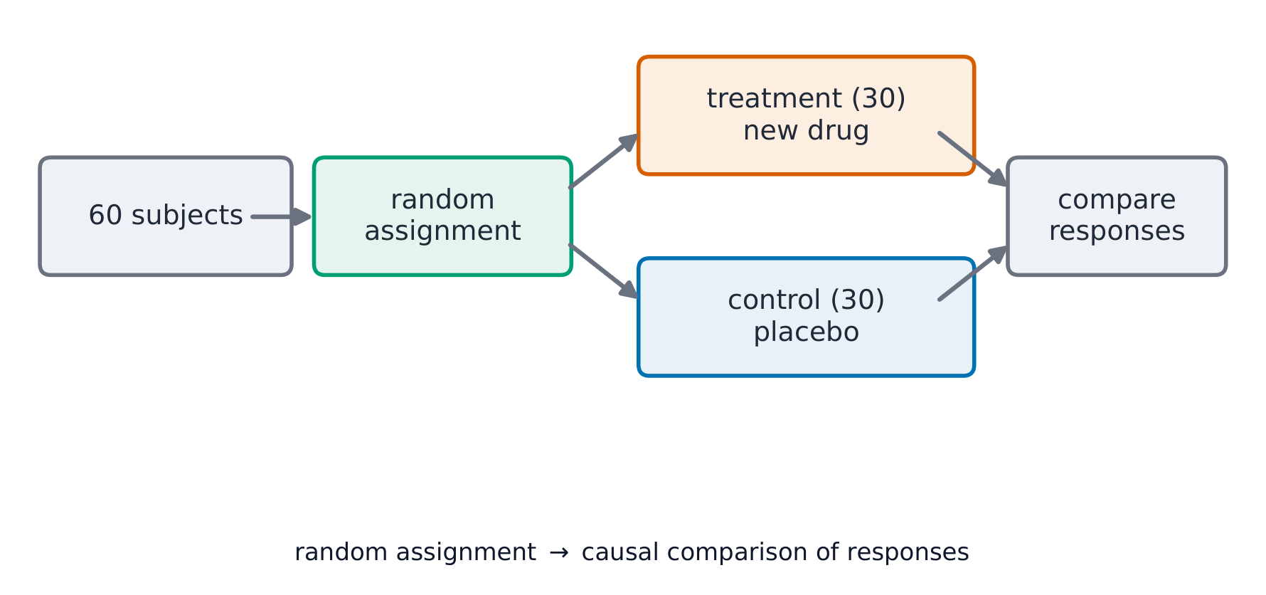
A completely randomized experiment compares a treatment group with a control group Confounding 混杂 occurs when another variable is tied to the treatment so their effects cannot be separated; random assignment guards against it. Blinding 盲法 hides who is getting which treatment to prevent expectation effects: in a single-blind 单盲 study only one side is kept unaware (usually the subjects, or only the people assessing the result), while in a double-blind 双盲 study neither the subjects nor the researchers who interact with them know, blocking both the placebo effect and biased assessment. Blocking 区组 groups similar subjects and randomizes within each block to reduce variability.

A clinical trial: random assignment separates treatment from control Vocabulary TrainEnglish control group/kənˈtrəʊl ɡruːp/ placebo/pləˈsiːbəʊ/ Random assignment/ˈrændəm əˈsaɪnmənt/ Replication/ˌreplɪˈkeɪʃn/ Confounding/kənˈfaʊndɪŋ/ Blinding/ˈblaɪndɪŋ/ single-blind/ˈsɪŋɡl blaɪnd/ double-blind/ˈdʌbl blaɪnd/ Blocking/ˈblɒkɪŋ/ 3.6
Choosing the Right Design
Syllabus
Enduring Understanding Learning Objective Essential Knowledge VAR-3
Well-designed experiments can establish evidence of causal relationships.VAR-3.D
Explain why a particular experimental design is appropriate. [Skill 1.C]- VAR-3.D.1 There are advantages and disadvantages for each experimental design depending on the question of interest, the resources available, and the nature of the experimental units.
Source: College Board AP Course and Exam Description
Match the design to the goal: use a completely randomized design for uniform subjects; a randomized block design when a known variable (sex, age) affects the response; a matched-pairs design when each subject can serve as its own control. State how you would carry out the randomization.
3.7
What an Experiment Lets You Conclude
Syllabus
Enduring Understanding Learning Objective Essential Knowledge VAR-3
Well-designed experiments can establish evidence of causal relationships.VAR-3.E
Interpret the results of a well-designed experiment. [Skill 4.B]- VAR-3.E.1 Statistical inference attributes conclusions based on data to the distribution from which the data were collected.
- VAR-3.E.2 Random assignment of treatments to experimental units allows researchers to conclude that some observed changes are so large as to be unlikely to have occurred by chance. Such changes are said to be statistically significant.
- VAR-3.E.3 Statistically significant differences between or among experimental treatment groups are evidence that the treatments caused the effect.
- VAR-3.E.4 If the experimental units used in an experiment are representative of some larger group of units, the results of an experiment can be generalized to the larger group. Random selection of experimental units gives a better chance that the units will be representative.
Source: College Board AP Course and Exam Description
Two questions decide the scope of a conclusion:
- Random assignment used? Then a significant difference can be attributed to the treatment (causation) – for these subjects.
- Random sampling from a population? Then results generalize to that population.
Only an experiment with random assignment supports a cause-and-effect claim; only random sampling supports generalization. Say exactly which you have.
Worked example. Researchers randomly assign $100$ volunteers to a new drug or a placebo, and the drug group improves significantly more. Because of the random assignment, the improvement can be attributed to the drug (causation) – but because the subjects were not randomly sampled, the conclusion applies only to these volunteers and does not automatically generalize to everyone.
3.7
Exam tips
- Distinguish an observational study (finds association) from an experiment (can show causation).
- Good sampling is random (SRS, stratified, cluster) — beware bias (voluntary response, undercoverage, nonresponse).
- Good experiments use control, randomization, and replication; blocking handles a known nuisance variable.
- Only a randomized experiment supports a cause-and-effect conclusion.
- Name the population, sample, and any confounding clearly.
-
4
Probability, Random Variables, and Probability Distributions
Watch lesson4.1
Random and Non-Random Patterns
Syllabus
Enduring Understanding Learning Objective Essential Knowledge VAR-1
Given that variation may be random or not, conclusions are uncertain.VAR-1.F
Identify questions suggested by patterns in data. [Skill 1.A]- VAR-1.F.1 Patterns in data do not necessarily mean that variation is not random.
Source: College Board AP Course and Exam Description
Something is random 随机 if individual outcomes are uncertain but a regular pattern emerges over many repetitions. Short-run results look erratic; long-run relative frequencies settle down. This long-run stability is what makes probability useful.
Vocabulary TrainEnglish random/ˈrændəm/ 4.2
Estimating Probabilities Using Simulation
Syllabus
Enduring Understanding Learning Objective Essential Knowledge UNC-2
Simulation allows us to anticipate patterns in data.UNC-2.A
Estimate probabilities using simulation. [Skill 3.A]- UNC-2.A.1 A random process generates results that are determined by chance.
- UNC-2.A.2 An outcome is the result of a trial of a random process.
- UNC-2.A.3 An event is a collection of outcomes.
- UNC-2.A.4 Simulation is a way to model random events, such that simulated outcomes closely match real-world outcomes. All possible outcomes are associated with a value to be determined by chance. Record the counts of simulated outcomes and the count total.
- UNC-2.A.5 The relative frequency of an outcome or event in simulated or empirical data can be used to estimate the probability of that outcome or event.
- UNC-2.A.6 The law of large numbers states that simulated (empirical) probabilities tend to get closer to the true probability as the number of trials increases.
- Illustrative examples for UNC-2.A:
- An outcome: Rolling a particular value on a six-sided number cube is one of six possible outcomes.
- An event: When rolling two six-sided number cubes, an event would be a sum of seven. The corresponding collection of outcomes would be $(1, 6)$, $(2, 5)$, $(3, 4)$, $(4, 3)$, $(5, 2)$, and $(6, 1)$, where the ordered pairs indicate (face value on one cube, face value on the other cube).
- Illustrative examples for UNC-2.A:
Source: College Board AP Course and Exam Description
A simulation 模拟 imitates a chance process using random digits or technology. Steps: state the model, assign digits to outcomes, run many trials, and record the proportion of trials meeting the condition. The resulting proportion estimates the probability – more trials give a better estimate.
Vocabulary TrainEnglish simulation/ˌsɪmjʊˈleɪʃn/ 4.3
Introduction to Probability

Syllabus
Enduring Understanding Learning Objective Essential Knowledge VAR-4
The likelihood of a random event can be quantified.VAR-4.A
Calculate probabilities for events and their complements. [Skill 3.A]- VAR-4.A.1 The sample space of a random process is the set of all possible non-overlapping outcomes.
- VAR-4.A.2 If all outcomes in the sample space are equally likely, then the probability an event E will occur is defined as the fraction: $\dfrac{\text{number of outcomes in event E}}{\text{total number of outcomes in sample space}}$
- VAR-4.A.3 The probability of an event is a number between 0 and 1, inclusive.
- VAR-4.A.4 The probability of the complement of an event E, $E'$ or $E^{C}$, (i.e., not E) is equal to $1 - P(E)$.
VAR-4.B
Interpret probabilities for events. [Skill 4.B]- VAR-4.B.1 Probabilities of events in repeatable situations can be interpreted as the relative frequency with which the event will occur in the long run.
Source: College Board AP Course and Exam Description
The probability 概率 of an event is a number from $0$ to $1$ giving its long-run relative frequency. The sample space 样本空间 is the set of all outcomes. For an event $A$, the complement 补 rule: $P(A^c)=1-P(A)$. Probabilities of all outcomes sum to $1$.
Probability runs from 0 (impossible) to 1 (certain) 
A deck of cards is a classic source of probability: 52 equally likely outcomes make the chances easy to count ExploreExplore probability with dice
Probability is the long-run fraction of times an outcome happens. Roll the dice many times and watch the experimental proportions settle toward the theoretical values.
Vocabulary TrainEnglish probability/ˌprɒbəˈbɪlɪti/ sample space/ˈsæmpl speɪs/ complement/ˈkɒmplɪmənt/ 4.4
Mutually Exclusive Events
Syllabus
Enduring Understanding Learning Objective Essential Knowledge VAR-4
The likelihood of a random event can be quantified.VAR-4.C
Explain why two events are (or are not) mutually exclusive. [Skill 4.B]- VAR-4.C.1 The probability that events $A$ and $B$ both will occur, sometimes called the joint probability, is the probability of the intersection of $A$ and $B$, denoted $P(A \cap B)$.
- VAR-4.C.2 Two events are mutually exclusive or disjoint if they cannot occur at the same time. So $P(A \cap B) = 0$.
Source: College Board AP Course and Exam Description
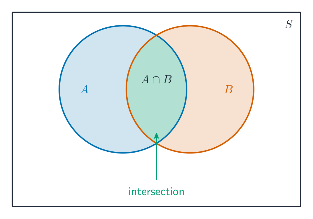
Two events are mutually exclusive 互斥 (disjoint) if they cannot both happen. Then the addition rule simplifies:
$$P(A\text{ or }B)=P(A)+P(B)\quad(\text{if mutually exclusive}).$$In general, $P(A\text{ or }B)=P(A)+P(B)-P(A\text{ and }B)$ – subtract the overlap so it is not counted twice.A Venn diagram: the overlap is the intersection of two events Vocabulary TrainEnglish mutually exclusive/ˈmjuːtʃuːəli eksˈkluːsɪv/ 4.5
Conditional Probability
Syllabus
Enduring Understanding Learning Objective Essential Knowledge VAR-4
The likelihood of a random event can be quantified.VAR-4.D
Calculate conditional probabilities. [Skill 3.A]- VAR-4.D.1 The probability that event $A$ will occur given that event $B$ has occurred is called a conditional probability and denoted $P(A \mid B) = \dfrac{P(A \cap B)}{P(B)}$.
- VAR-4.D.2 The multiplication rule states that the probability that events $A$ and $B$ both will occur is equal to the probability that event $A$ will occur multiplied by the probability that event $B$ will occur, given that $A$ has occurred. This is denoted $P(A \cap B) = P(A) \cdot P(B \mid A)$.
Source: College Board AP Course and Exam Description
Conditional probability The conditional probability 条件概率 of $A$ given $B$ is
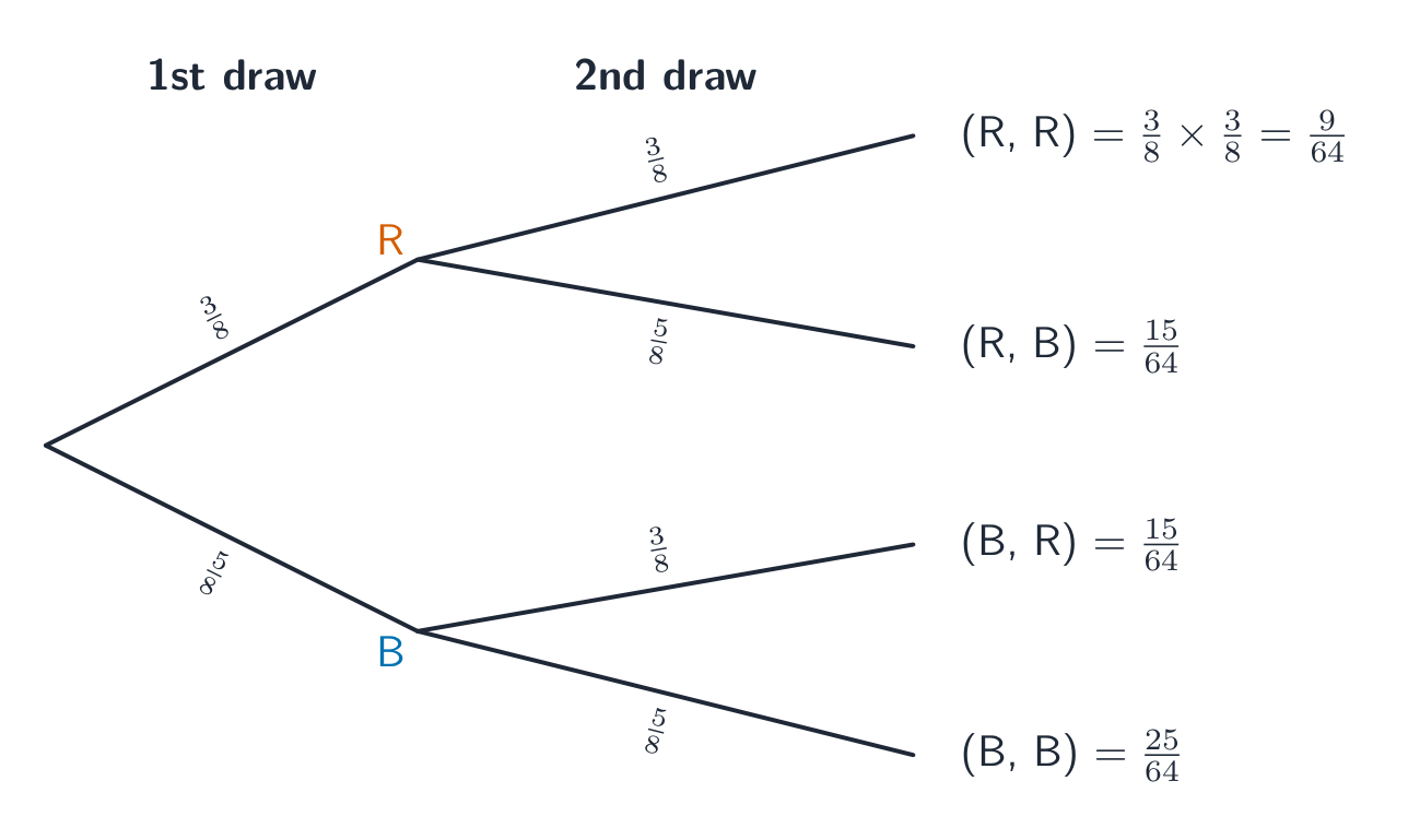
$$P(A\mid B)=\frac{P(A\text{ and }B)}{P(B)}.$$It is the chance of $A$ once you know $B$ happened. Two-way tables make these easy: restrict to the row/column for $B$, then find $A$'s share.On a tree diagram, multiply the probabilities along the branches ExploreUpdate a probability on new information
Conditional probability $P(B\mid A)$ is the chance of $B$ once you know $A$ happened. Change the branch probabilities and watch how conditioning reshapes the outcome.
Vocabulary TrainEnglish conditional probability/kənˈdɪʃənl ˌprɒbəˈbɪlɪti/ 4.6
Independent Events and Unions of Events
Syllabus
Enduring Understanding Learning Objective Essential Knowledge VAR-4
The likelihood of a random event can be quantified.VAR-4.E
Calculate probabilities for independent events and for the union of two events. [Skill 3.A]- VAR-4.E.1 Events $A$ and $B$ are independent if, and only if, knowing whether event $A$ has occurred (or will occur) does not change the probability that event $B$ will occur.
- VAR-4.E.2 If, and only if, events $A$ and $B$ are independent, then $P(A \mid B) = P(A)$, $P(B \mid A) = P(B)$, and $P(A \cap B) = P(A) \cdot P(B)$.
- VAR-4.E.3 The probability that event $A$ or event $B$ (or both) will occur is the probability of the union of $A$ and $B$, denoted $P(A \cup B)$.
- VAR-4.E.4 The addition rule states that the probability that event $A$ or event $B$ or both will occur is equal to the probability that event $A$ will occur plus the probability that event $B$ will occur minus the probability that both events $A$ and $B$ will occur. This is denoted $P(A \cup B) = P(A) + P(B) - P(A \cap B)$.
Source: College Board AP Course and Exam Description
Events are independent 独立 if knowing one does not change the other's probability: $P(A\mid B)=P(A)$. Then the multiplication rule simplifies:
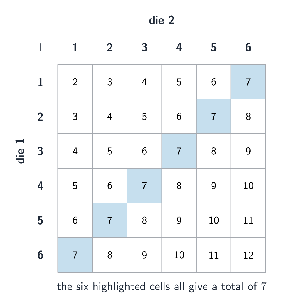
$$P(A\text{ and }B)=P(A)\,P(B)\quad(\text{if independent}).$$Independent is not the same as mutually exclusive – mutually exclusive events with nonzero probability are actually dependent (if one happens, the other cannot).A sample space diagram lists every equally likely outcome ExploreCombine events with a Venn diagram
For a union $P(A\cup B)=P(A)+P(B)-P(A\cap B)$ — you subtract the overlap so it isn't counted twice. Switch the operation to see each region light up.
Vocabulary TrainEnglish independent/ˌɪndɪˈpendənt/ 4.7
Random Variables and Probability Distributions
Syllabus
Enduring Understanding Learning Objective Essential Knowledge VAR-5
Probability distributions may be used to model variation in populations.VAR-5.A
Represent the probability distribution for a discrete random variable. [Skill 2.B]- VAR-5.A.1 The values of a random variable are the numerical outcomes of random behavior.
- VAR-5.A.2 A discrete random variable is a variable that can only take a countable number of values. Each value has a probability associated with it. The sum of the probabilities over all of the possible values must be 1.
- VAR-5.A.3 A probability distribution can be represented as a graph, table, or function showing the probabilities associated with values of a random variable.
- VAR-5.A.4 A cumulative probability distribution can be represented as a table or function showing the probability of being less than or equal to each value of the random variable.
- Illustrative examples for VAR-5.A: Outcomes of trials of a random process:
- The sum of the outcomes for rolling two dice
- The number of puppies in a randomly selected litter for a certain breed of dog
- Illustrative examples for VAR-5.A: Outcomes of trials of a random process:
VAR-5.B
Interpret a probability distribution. [Skill 4.B]- VAR-5.B.1 An interpretation of a probability distribution provides information about the shape, center, and spread of a population and allows one to make conclusions about the population of interest.
Source: College Board AP Course and Exam Description
A random variable 随机变量 assigns a number to each outcome of a chance process. A probability distribution 概率分布 lists each possible value with its probability (they sum to $1$). A distribution can be discrete (a table of values) or continuous (an area-under-a-curve model like the normal).
Vocabulary TrainEnglish random variable/ˈrændəm ˈveərɪəbl/ probability distribution/ˌprɒbəˈbɪlɪti ˌdɪstrɪˈbjuːʃn/ 4.8
Mean and Standard Deviation of Random Variables
Syllabus
Enduring Understanding Learning Objective Essential Knowledge VAR-5
Probability distributions may be used to model variation in populations.VAR-5.C
Calculate parameters for a discrete random variable. [Skill 3.B]- VAR-5.C.1 A numerical value measuring a characteristic of a population or the distribution of a random variable is known as a parameter, which is a single, fixed value.
- VAR-5.C.2 The mean, or expected value, for a discrete random variable $X$ is $\mu_X = \sum x_i \cdot P(x_i)$.
- VAR-5.C.3 The standard deviation for a discrete random variable $X$ is $\sigma_X = \sqrt{\sum (x_i - \mu_x)^2 \cdot P(x_i)}$.
VAR-5.D
Interpret parameters for a discrete random variable. [Skill 4.B]- VAR-5.D.1 Parameters for a discrete random variable should be interpreted using appropriate units and within the context of a specific population.
Source: College Board AP Course and Exam Description
The mean (expected value) 期望值 of a discrete random variable is the probability-weighted average:
$$\mu_X=E(X)=\sum x_i\,P(x_i).$$The standard deviation $\sigma_X=\sqrt{\sum (x_i-\mu_X)^2\,P(x_i)}$ measures typical spread from the mean. The expected value is the long-run average outcome, not a value you expect on any single trial.Worked example. A game pays $\$5$ with probability $0.2$ and costs you $\$1$ (a $-1$ outcome) with probability $0.8$. The expected value is
$$E(X)=5(0.2)+(-1)(0.8)=1-0.8=\$0.20,$$so over many plays you gain about $20$ cents per play on average, even though no single play gives exactly that.Vocabulary TrainEnglish mean (expected value)/miːn/ 4.9
Combining Random Variables
Syllabus
Enduring Understanding Learning Objective Essential Knowledge VAR-5
Probability distributions may be used to model variation in populations.VAR-5.E
Calculate parameters for linear combinations of random variables. [Skill 3.B]- VAR-5.E.1 For random variables $X$ and $Y$ and real numbers $a$ and $b$, the mean of $aX + bY$ is $a\mu_x + b\mu_y$.
- VAR-5.E.2 Two random variables are independent if knowing information about one of them does not change the probability distribution of the other.
- VAR-5.E.3 For independent random variables $X$ and $Y$ and real numbers $a$ and $b$, the mean of $aX + bY$ is $a\mu_x + b\mu_y$, and the variance of $aX + bY$ is $a^2\sigma^2_x + b^2\sigma^2_y$.
VAR-5.F
Describe the effects of linear transformations of parameters of random variables. [Skill 3.C]- VAR-5.F.1 For $Y = a + bX$, the probability distribution of the transformed random variable, $Y$, has the same shape as the probability distribution for $X$, so long as $a > 0$ and $b > 0$. The mean of $Y$ is $\mu_y = a + b\mu_x$. The standard deviation of $Y$ is $\sigma_y = |b|\sigma_x$.
Source: College Board AP Course and Exam Description
When you add or subtract random variables, means add: $\mu_{X\pm Y}=\mu_X\pm\mu_Y$. If $X$ and $Y$ are independent, variances add (even when subtracting):
$$\sigma^2_{X\pm Y}=\sigma^2_X+\sigma^2_Y.$$Take the square root for the standard deviation. Also, scaling: $\mu_{aX+b}=a\mu_X+b$ and $\sigma_{aX+b}=|a|\sigma_X$.4.10
Introduction to the Binomial Distribution
Syllabus
Enduring Understanding Learning Objective Essential Knowledge UNC-3
Probabilistic reasoning allows us to anticipate patterns in data.UNC-3.A
Estimate probabilities of binomial random variables using data from a simulation. [Skill 3.A]- UNC-3.A.1 A probability distribution can be constructed using the rules of probability or estimated with a simulation using random number generators.
- UNC-3.A.2 A binomial random variable, $X$, counts the number of successes in $n$ repeated independent trials, each trial having two possible outcomes (success or failure), with the probability of success $p$ and the probability of failure $1 - p$.
UNC-3.B
Calculate probabilities for a binomial distribution. [Skill 3.A]- UNC-3.B.1 The probability that a binomial random variable, $X$, has exactly $x$ successes for $n$ independent trials, when the probability of success is $p$, is calculated as $P(X = x) = \binom{n}{x} p^x (1 - p)^{n-x}, x = 0, 1, 2, \ldots, n$. This is the binomial probability function.
Source: College Board AP Course and Exam Description
The binomial distribution A binomial 二项 setting (BINS): a fixed number $n$ of Independent trials, each with two outcomes (success/failure) and the same success probability $p$. The random variable $X=$ number of successes. Its probability:
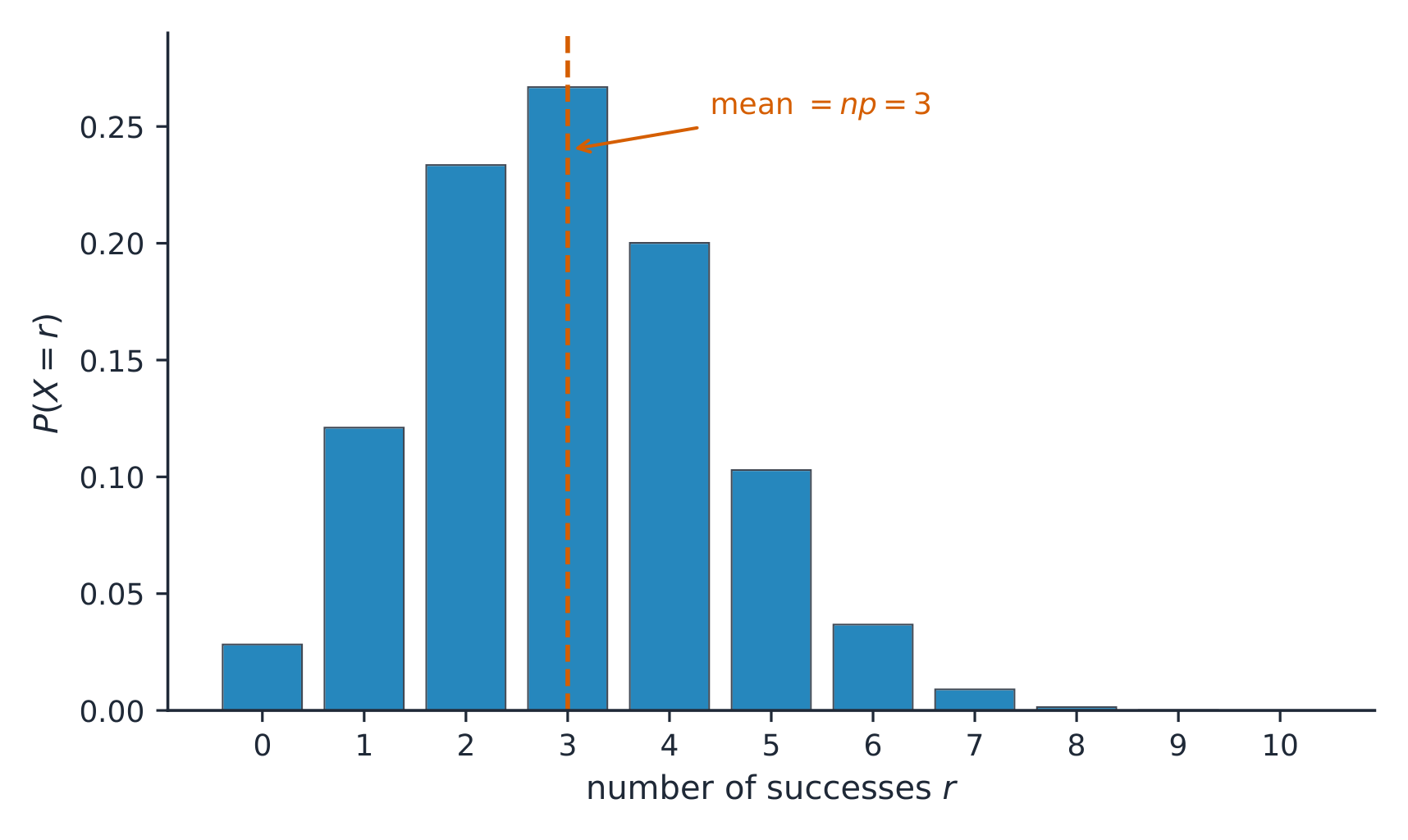
$$P(X=k)=\binom{n}{k}p^k(1-p)^{n-k}.$$The binomial distribution, with mean n times p ExploreShape a binomial distribution
A binomial distribution counts successes in $n$ independent trials each with probability $p$. Change $n$ and $p$ and watch the bars shift and spread.
Vocabulary TrainEnglish binomial/baɪˈnəʊmɪəl/ 4.11
Parameters for a Binomial Distribution
Syllabus
Enduring Understanding Learning Objective Essential Knowledge UNC-3
Probabilistic reasoning allows us to anticipate patterns in data.UNC-3.C
Calculate parameters for a binomial distribution. [Skill 3.B]- UNC-3.C.1 If a random variable is binomial, its mean, $\mu_x$, is $np$ and its standard deviation, $\sigma_x$, is $\sqrt{np(1 - p)}$.
UNC-3.D
Interpret probabilities and parameters for a binomial distribution. [Skill 4.B]- UNC-3.D.1 Probabilities and parameters for a binomial distribution should be interpreted using appropriate units and within the context of a specific population or situation.
Source: College Board AP Course and Exam Description
For a binomial $X$ with $n$ trials and success probability $p$:
$$\mu_X=np,\qquad \sigma_X=\sqrt{np(1-p)}.$$Use these for "how many successes do we expect, and how much do they vary" questions.Worked example. A player makes $70\%$ of free throws. In $n=10$ shots, the probability of exactly $8$ makes is
$$P(X=8)=\binom{10}{8}(0.7)^8(0.3)^2=45\times0.0576\times0.09\approx0.23,$$and the expected number of makes is $\mu=np=10(0.7)=7$, with $\sigma=\sqrt{10(0.7)(0.3)}\approx1.45$.4.12
The Geometric Distribution
Syllabus
Enduring Understanding Learning Objective Essential Knowledge UNC-3
Probabilistic reasoning allows us to anticipate patterns in data.UNC-3.E
Calculate probabilities for geometric random variables. [Skill 3.A]- UNC-3.E.1 For a sequence of independent trials, a geometric random variable, $X$, gives the number of the trial on which the first success occurs. Each trial has two possible outcomes (success or failure) with the probability of success $p$ and the probability of failure $1 - p$.
- UNC-3.E.2 The probability that the first success for repeated independent trials with probability of success $p$ occurs on trial $x$ is calculated as $P(X = x) = (1 - p)^{x-1} p, x = 1, 2, 3, \ldots$. This is the geometric probability function.
UNC-3.F
Calculate parameters of a geometric distribution. [Skill 3.B]- UNC-3.F.1 If a random variable is geometric, its mean, $\mu_x$, is $\dfrac{1}{p}$ and its standard deviation, $\sigma_x$, is $\dfrac{\sqrt{(1 - p)}}{p}$.
UNC-3.G
Interpret probabilities and parameters for a geometric distribution. [Skill 4.B]- UNC-3.G.1 Probabilities and parameters for a geometric distribution should be interpreted using appropriate units and within the context of a specific population or situation.
Source: College Board AP Course and Exam Description
A geometric 几何 setting is the same as binomial but with no fixed $n$: you keep trying until the first success. The random variable $Y=$ the trial of the first success:
$$P(Y=k)=(1-p)^{k-1}\,p,\qquad \mu_Y=\frac{1}{p}.$$So the expected number of trials until the first success is $1/p$.Vocabulary TrainEnglish geometric/ˌdʒiːəʊˈmetrɪk/ 4.12
Exam tips
- A probability lies in $[0,1]$; use the complement ($1-P$) and add mutually exclusive events.
- For independent events multiply; for "and/or" use the general addition and conditional rules.
- Expected value = $\sum(\text{value}\times\text{probability})$.
- Recognise binomial (fixed $n$, two outcomes, constant $p$) and geometric settings.
- Draw a tree or table for multi-stage problems and multiply along branches.
-
5
Sampling Distributions
Watch lesson5.1
Why Two Samples Never Match: Sampling Variability
Syllabus
Enduring Understanding Learning Objective Essential Knowledge VAR-1
Given that variation may be random or not, conclusions are uncertain.VAR-1.G
Identify questions suggested by variation in statistics for samples collected from the same population. [Skill 1.A]- VAR-1.G.1 Variation in statistics for samples taken from the same population may be random or not.
Source: College Board AP Course and Exam Description
A statistic 统计量 (like a sample mean $\bar{x}$ or sample proportion $\hat{p}$) is computed from a sample and varies from sample to sample – this is sampling variability 抽样变异. A parameter 参数 ($\mu$ or $p$) is the fixed truth about the population. The sampling distribution 抽样分布 is the distribution of a statistic over all possible samples of a given size – it is the bridge from one sample to inference.
Vocabulary TrainEnglish statistic/stəˈtɪstɪk/ sampling variability/ˈsæmplɪŋ ˌveərɪəˈbɪlɪti/ parameter/pəˈræmɪtə/ sampling distribution/ˈsæmplɪŋ ˌdɪstrɪˈbjuːʃn/ 5.2
The Normal Curve as a Model for a Statistic
Syllabus
Enduring Understanding Learning Objective Essential Knowledge VAR-6
The normal distribution may be used to model variation.VAR-6.A
Calculate the probability that a particular value lies in a given interval of a normal distribution. [Skill 3.A]- VAR-6.A.1 A continuous random variable is a variable that can take on any value within a specified domain. Every interval within the domain has a probability associated with it.
- VAR-6.A.2 A continuous random variable with a normal distribution is commonly used to describe populations. The distribution of a normal random variable can be described by a normal, or "bell-shaped," curve.
- VAR-6.A.3 The area under a normal curve over a given interval represents the probability that a particular value lies in that interval.
- Illustrative examples for VAR-6.A: Continuous random variable: If one looks at a clock at a random time, the probability that the minute hand is between the 3 and the 6 is one fourth.
VAR-6.B
Determine the interval associated with a given area in a normal distribution. [Skill 3.A]- VAR-6.B.1 The boundaries of an interval associated with a given area in a normal distribution can be determined using $z$-scores or technology, such as a calculator, a standard normal table, or computer-generated output.
- VAR-6.B.2 Intervals associated with a given area in a normal distribution can be determined by assigning appropriate inequalities to the boundaries of the intervals:
- a. $P(X < x_a) = \dfrac{p}{100}$ means that the lowest $p\%$ of values lie to the left of $x_a$.
- b. $P(x_a < X < x_b) = \dfrac{p}{100}$ means that $p\%$ of values lie between $x_a$ and $x_b$.
- c. $P(X > x_b) = \dfrac{p}{100}$ means that the highest $p\%$ of values lie to the right of $x_b$.
- d. To determine the most extreme $p\%$ of values requires dividing the area associated with $p\%$ into two equal areas on either extreme of the distribution: $P(X < x_a) = \dfrac{1}{2}\dfrac{p}{100}$ and $P(X > x_b) = \dfrac{1}{2}\dfrac{p}{100}$ means that half of the $p\%$ most extreme values lie to the left of $x_a$ and half of the $p\%$ most extreme values lie to the right of $x_b$.
VAR-6.C
Determine the appropriateness of using the normal distribution to approximate probabilities for unknown distributions. [Skill 3.C]- VAR-6.C.1 Normal distributions are symmetrical and "bell-shaped." As a result, normal distributions can be used to approximate distributions with similar characteristics.
Source: College Board AP Course and Exam Description
The normal distribution For large enough samples, many sampling distributions are approximately normal. That lets us describe a statistic by a center (its mean), a spread (its standard error 标准误), and a normal shape – and then compute how likely a given sample result is.
ExploreUse the normal curve to find a proportion
A normal model turns a range of values into an area = a proportion. Shade a band to read off the fraction of samples falling within it (the 68-95-99.7 rule).
Vocabulary TrainEnglish standard error/ˈstændəd ˈerə/ 5.3
The Central Limit Theorem
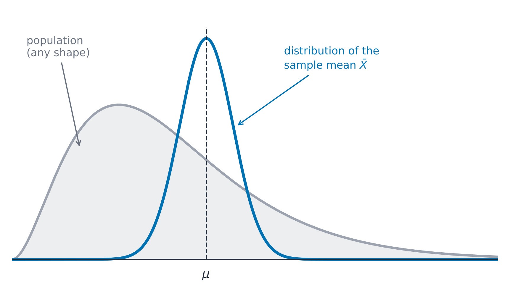
Syllabus
Enduring Understanding Learning Objective Essential Knowledge UNC-3
Probabilistic reasoning allows us to anticipate patterns in data.UNC-3.H
Estimate sampling distributions using simulation. [Skill 3.C]- UNC-3.H.1 A sampling distribution of a statistic is the distribution of values for the statistic for all possible samples of a given size from a given population.
- UNC-3.H.2 The central limit theorem (CLT) states that when the sample size is sufficiently large, a sampling distribution of the mean of a random variable will be approximately normally distributed.
- UNC-3.H.3 The central limit theorem requires that the sample values are independent of each other and that $n$ is sufficiently large.
- UNC-3.H.4 A randomization distribution is a collection of statistics generated by simulation assuming known values for the parameters. For a randomized experiment, this means repeatedly randomly reallocating/reassigning the response values to treatment groups.
- UNC-3.H.5 The sampling distribution of a statistic can be simulated by generating repeated random samples from a population.
Source: College Board AP Course and Exam Description
The Central Limit Theorem The Central Limit Theorem 中心极限定理 (CLT): for a sample mean, if the sample size $n$ is large enough (a common rule is $n\ge 30$), the sampling distribution of $\bar{x}$ is approximately normal, regardless of the population's shape. The larger $n$, the more normal and the tighter the distribution.
The sample mean is nearly normal whatever the shape of the population ExploreWatch a sampling distribution turn normal
The Central Limit Theorem: for a large enough sample, the distribution of the sample mean is approximately normal — whatever the shape of the population.
Vocabulary TrainEnglish Central Limit Theorem/ˈsentrəl ˈlɪmɪt ˈθɪərəm/ 5.4
Good Guesses and Bad Guesses: Bias
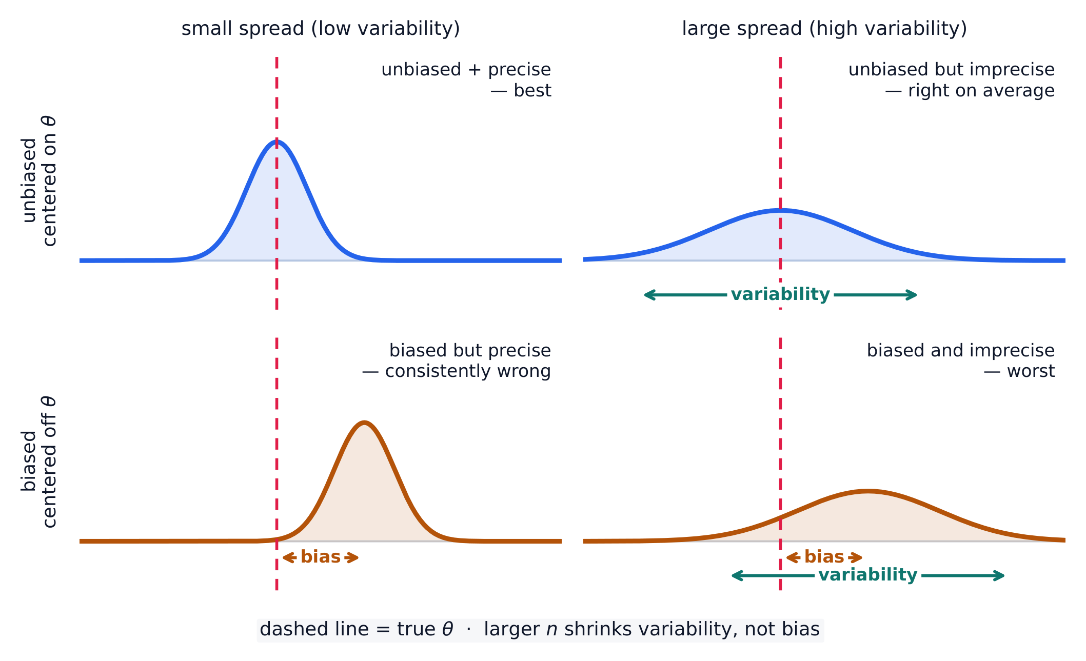
Syllabus
Enduring Understanding Learning Objective Essential Knowledge UNC-3
Probabilistic reasoning allows us to anticipate patterns in data.UNC-3.I
Explain why an estimator is or is not unbiased. [Skill 4.B]- UNC-3.I.1 When estimating a population parameter, an estimator is unbiased if, on average, the value of the estimator is equal to the population parameter.
UNC-3.J
Calculate estimates for a population parameter. [Skill 3.B]- UNC-3.J.1 When estimating a population parameter, an estimator exhibits variability that can be modeled using probability.
- UNC-3.J.2 A sample statistic is a point estimator of the corresponding population parameter.
Source: College Board AP Course and Exam Description
A statistic is unbiased 无偏 if the mean of its sampling distribution equals the parameter – it is correct on average. Bias is about the center being off; variability is about the spread. A good estimator is both unbiased (centered right) and low-variability (precise); larger samples reduce variability but do not fix bias from bad sampling.
Bias and variability are separate faults. Only the top-left estimator is both centered on $\theta$ and tight; the bottom-left one is precise but consistently wrong, which no amount of extra data will fix. Vocabulary TrainEnglish unbiased/ʌnˈbaɪəst/ 5.5
The Sampling Distribution of a Sample Proportion
Syllabus
Enduring Understanding Learning Objective Essential Knowledge UNC-3
Probabilistic reasoning allows us to anticipate patterns in data.UNC-3.K
Determine parameters of a sampling distribution for sample proportions. [Skill 3.B]- UNC-3.K.1 For independent samples (sampling with replacement) of a categorical variable from a population with population proportion, $p$, the sampling distribution of the sample proportion, $\hat{p}$, has a mean, $\mu_{\hat{p}} = p$ and a standard deviation, $\sigma_{\hat{p}} = \sqrt{\dfrac{p(1-p)}{n}}$.
- UNC-3.K.2 If sampling without replacement, the standard deviation of the sample proportion is smaller than what is given by the formula above. If the sample size is less than 10% of the population size, the difference is negligible.
UNC-3.L
Determine whether a sampling distribution for a sample proportion can be described as approximately normal. [Skill 3.C]- UNC-3.L.1 For a categorical variable, the sampling distribution of the sample proportion, $\hat{p}$, will have an approximate normal distribution, provided the sample size is large enough: $np \geq 10$ and $n(1-p) \geq 10$
UNC-3.M
Interpret probabilities and parameters for a sampling distribution for a sample proportion. [Skill 4.B]- UNC-3.M.1 Probabilities and parameters for a sampling distribution for a sample proportion should be interpreted using appropriate units and within the context of a specific population.
Source: College Board AP Course and Exam Description
For a sample proportion $\hat{p}$ from an SRS: the mean is $p$ (unbiased), and the standard deviation is
$$\sigma_{\hat p}=\sqrt{\frac{p(1-p)}{n}}.$$This spread has two names: it is the standard deviation of the sampling distribution, and it is called the standard error once you must estimate it from the sample (replacing $p$ by $\hat p$) — which is exactly what the later inference units do. It is approximately normal when $np\ge 10$ and $n(1-p)\ge 10$ (the Large Counts condition), and the $10\%$ condition ($n\le 0.10N$) keeps the observations near-independent.Worked example. Suppose $40\%$ of voters favor a measure ($p=0.4$) and you sample $n=100$. The standard error is $\sigma_{\hat p}=\sqrt{\dfrac{0.4(0.6)}{100}}=0.049$. The chance a sample gives $\hat{p}>0.5$ is $z=\dfrac{0.5-0.4}{0.049}=2.04$, so $P(\hat p>0.5)\approx0.02$ – a majority in the sample would be surprising.
5.6
Comparing Two Groups: Difference of Sample Proportions
Syllabus
Enduring Understanding Learning Objective Essential Knowledge UNC-3
Probabilistic reasoning allows us to anticipate patterns in data.UNC-3.N
Determine parameters of a sampling distribution for a difference in sample proportions. [Skill 3.B]- UNC-3.N.1 For a categorical variable, when randomly sampling with replacement from two independent populations with population proportions $p_1$ and $p_2$, the sampling distribution of the difference in sample proportions $\hat{p}_1 - \hat{p}_2$ has mean, $\mu_{\hat{p}_1 - \hat{p}_2} = p_1 - p_2$ and standard deviation, $\sigma_{\hat{p}_1 - \hat{p}_2} = \sqrt{\dfrac{p_1(1-p_1)}{n_1} + \dfrac{p_2(1-p_2)}{n_2}}$.
- UNC-3.N.2 If sampling without replacement, the standard deviation of the difference in sample proportions is smaller than what is given by the formula above. If the sample sizes are less than 10% of the population sizes, the difference is negligible.
UNC-3.O
Determine whether a sampling distribution for a difference of sample proportions can be described as approximately normal. [Skill 3.C]- UNC-3.O.1 The sampling distribution of the difference in sample proportions $\hat{p}_1 - \hat{p}_2$ will have an approximate normal distribution provided the sample sizes are large enough: $n_1 p_1 \geq 10, n_1(1-p_1) \geq 10, n_2 p_2 \geq 10, n_2(1-p_2) \geq 10$.
UNC-3.P
Interpret probabilities and parameters for a sampling distribution for a difference in proportions. [Skill 4.B]- UNC-3.P.1 Parameters for a sampling distribution for a difference of proportions should be interpreted using appropriate units and within the context of a specific populations.
Source: College Board AP Course and Exam Description
For $\hat{p}_1-\hat{p}_2$ from two independent samples: the mean is $p_1-p_2$, and because the samples are independent the variances add:
$$\sigma_{\hat p_1-\hat p_2}=\sqrt{\frac{p_1(1-p_1)}{n_1}+\frac{p_2(1-p_2)}{n_2}}.$$It is approximately normal when the Large Counts condition holds in both samples.5.7
The Sampling Distribution of a Sample Mean
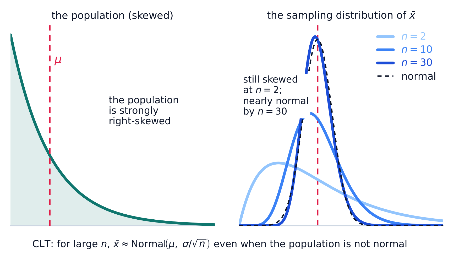
Syllabus
Enduring Understanding Learning Objective Essential Knowledge UNC-3
Probabilistic reasoning allows us to anticipate patterns in data.UNC-3.Q
Determine parameters for a sampling distribution for sample means. [Skill 3.B]- UNC-3.Q.1 For a numerical variable, when random sampling with replacement from a population with mean $\mu$ and standard deviation, $\sigma$, the sampling distribution of the sample mean has mean $\mu_{\bar{x}} = \mu$ and standard deviation $\sigma_{\bar{x}} = \dfrac{\sigma}{\sqrt{n}}$.
- UNC-3.Q.2 If sampling without replacement, the standard deviation of the sample mean is smaller than what is given by the formula above. If the sample size is less than 10% of the population size, the difference is negligible.
UNC-3.R
Determine whether a sampling distribution of a sample mean can be described as approximately normal. [Skill 3.C]- UNC-3.R.1 For a numerical variable, if the population distribution can be modeled with a normal distribution, the sampling distribution of the sample mean, $\bar{x}$, can be modeled with a normal distribution.
- UNC-3.R.2 For a numerical variable, if the population distribution cannot be modeled with a normal distribution, the sampling distribution of the sample mean, $\bar{x}$, can be modeled approximately by a normal distribution, provided the sample size is large enough, e.g., greater than or equal to 30.
UNC-3.S
Interpret probabilities and parameters for a sampling distribution for a sample mean. [Skill 4.B]- UNC-3.S.1 Probabilities and parameters for a sampling distribution for a sample mean should be interpreted using appropriate units and within the context of a specific population.
Source: College Board AP Course and Exam Description
For a sample mean $\bar{x}$ from an SRS: the mean is $\mu$ (unbiased), and the standard deviation is
$$\sigma_{\bar x}=\frac{\sigma}{\sqrt{n}}.$$Its shape is normal if the population is normal, or approximately normal for large $n$ by the CLT. Note the spread shrinks like $\sqrt{n}$ – quadrupling the sample halves the standard error.Worked example. A population has $\mu=70$ and $\sigma=12$. For samples of $n=36$, the sampling distribution of $\bar{x}$ is centered at $70$ with standard error $\dfrac{12}{\sqrt{36}}=2$. The chance a sample mean exceeds $73$ is $z=\dfrac{73-70}{2}=1.5$, so $P(\bar x>73)\approx0.067$.
The population on the left is strongly skewed, yet every sampling distribution of $\bar{x}$ is centered at $\mu$. A larger $n$ shrinks the standard error $\sigma/\sqrt{n}$, so the curve gets taller and narrower – and it also straightens: still clearly skewed at $n=2$, almost exactly normal (dashed) by $n=30$. 5.8
Comparing Two Groups: Difference of Sample Means
Syllabus
Enduring Understanding Learning Objective Essential Knowledge UNC-3
Probabilistic reasoning allows us to anticipate patterns in data.UNC-3.T
Determine parameters of a sampling distribution for a difference in sample means. [Skill 3.B]- UNC-3.T.1 For a numerical variable, when randomly sampling with replacement from two independent populations with population means $\mu_1$ and $\mu_2$ and population standard deviations $\sigma_1$ and $\sigma_2$, the sampling distribution of the difference in sample means $\bar{x}_1 - \bar{x}_2$ has mean $\mu_{(\bar{x}_1 - \bar{x}_2)} = \mu_1 - \mu_2$ and standard deviation, $\sigma_{(\bar{x}_1 - \bar{x}_2)} = \sqrt{\dfrac{\sigma_1^2}{n_1} + \dfrac{\sigma_2^2}{n_2}}$.
- UNC-3.T.2 If sampling without replacement, the standard deviation of the difference in sample means is smaller than what is given by the formula above. If the sample sizes are less than 10% of the population sizes, the difference is negligible.
UNC-3.U
Determine whether a sampling distribution of a difference in sample means can be described as approximately normal. [Skill 3.C]- UNC-3.U.1 The sampling distribution of the difference in sample means $\bar{x}_1 - \bar{x}_2$ can be modeled with a normal distribution if the two population distributions can be modeled with a normal distribution.
- UNC-3.U.2 The sampling distribution of the difference in sample means $\bar{x}_1 - \bar{x}_2$ can be modeled approximately by a normal distribution if the two population distributions cannot be modeled with a normal distribution but both sample sizes are greater than or equal to 30.
UNC-3.V
Interpret probabilities and parameters for a sampling distribution for a difference in sample means. [Skill 4.B]- UNC-3.V.1 Probabilities and parameters for a sampling distribution for a difference of sample means should be interpreted using appropriate units and within the context of a specific populations.
Source: College Board AP Course and Exam Description
For $\bar{x}_1-\bar{x}_2$ from two independent samples: the mean is $\mu_1-\mu_2$, and (independent, so variances add)
$$\sigma_{\bar x_1-\bar x_2}=\sqrt{\frac{\sigma_1^2}{n_1}+\frac{\sigma_2^2}{n_2}}.$$This is the foundation for two-sample inference in the next units.5.8
Exam tips
- A sampling distribution is the distribution of a statistic over many samples, centered on the true parameter.
- The Central Limit Theorem: for a large enough sample the sample mean is approximately normal, even if the population is not.
- Larger samples give less variability (a smaller standard error).
- Check the conditions (random, independent/10%, large enough) before using a normal model.
- Keep straight what varies — the statistic — versus the fixed parameter.
-
6
Inference for Categorical Data: Proportions
Watch lesson6.1
Why Be Normal?
Syllabus
Enduring Understanding Learning Objective Essential Knowledge VAR-1
Given that variation may be random or not, conclusions are uncertain.VAR-1.H
Identify questions suggested by variation in the shapes of distributions of samples taken from the same population. [Skill 1.A]- VAR-1.H.1 Variation in shapes of data distributions may be random or not.
Source: College Board AP Course and Exam Description
Because a sample proportion $\hat{p}$ is approximately normally distributed (when the conditions hold), we can measure how far a sample result is from a claimed value in standard errors, and turn that into a probability. This is what makes inference 推断 – drawing conclusions about a population from a sample – possible.
Vocabulary TrainEnglish inference/ˈɪnfərəns/ 6.2
Confidence Interval for a Proportion
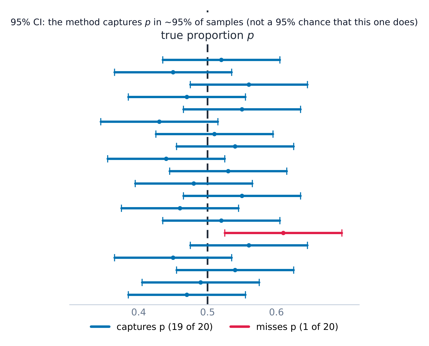
Syllabus
Enduring Understanding Learning Objective Essential Knowledge UNC-4
An interval of values should be used to estimate parameters, in order to account for uncertainty.UNC-4.A
Identify an appropriate confidence interval procedure for a population proportion. [Skill 1.D]- UNC-4.A.1 The appropriate confidence interval procedure for a one-sample proportion for one categorical variable is a one sample $z$-interval for a proportion.
UNC-4.B
Verify the conditions for calculating confidence intervals for a population proportion. [Skill 4.C]- UNC-4.B.1 In order to make assumptions necessary for inference on population proportions, means, and slopes, we must check for independence in data collection methods and for selection of the appropriate sampling distribution.
- UNC-4.B.2 In order to calculate a confidence interval to estimate a population proportion, $p$, we must check for independence and that the sampling distribution is approximately normal.
- a. To check for independence:
- i. Data should be collected using a random sample or a randomized experiment.
- ii. When sampling without replacement, check that $n \leq 10\%N$, where $N$ is the size of the population.
- b. To check that the sampling distribution of $\hat{p}$ is approximately normal (shape):
- i. For categorical variables, check that both the number of successes, $n\hat{p}$, and the number of failures, $n(1-\hat{p})$ are at least 10 so that the sample size is large enough to support an assumption of normality.
- a. To check for independence:
UNC-4.C
Determine the margin of error for a given sample size and an estimate for the sample size that will result in a given margin of error for a population proportion. [Skill 3.D]- UNC-4.C.1 Based on sample data, the standard error of a statistic is an estimate for the standard deviation for the statistic. The standard error of $\hat{p}$ is $SE_{\hat{p}} = \sqrt{\dfrac{\hat{p}(1-\hat{p})}{n}}$.
- UNC-4.C.2 A margin of error gives how much a value of a sample statistic is likely to vary from the value of the corresponding population parameter.
- UNC-4.C.3 For categorical variables, the margin of error is the critical value ($z^*$) times the standard error (SE) of the relevant statistic, which equals $z^* \sqrt{\dfrac{\hat{p}(1-\hat{p})}{n}}$ for a one sample proportion.
- UNC-4.C.4 The formula for margin of error can be rearranged to solve for $n$, the minimum sample size needed to achieve a given margin of error. For this purpose, use a guess for $\hat{p}$ or use $\hat{p} = 0.5$ in order to find an upper bound for the sample size that will result in a given margin of error.
UNC-4.D
Calculate an appropriate confidence interval for a population proportion. [Skill 3.D]- UNC-4.D.1 In general, an interval estimate can be constructed as point estimate ± (margin of error). For a one-sample proportion, the interval estimate is $\hat{p} \pm z^* \sqrt{\dfrac{\hat{p}(1-\hat{p})}{n}}$.
- Clarifying statement: Formulas for interval estimates do not appear explicitly on the AP Statistics Formula Sheet provided with the AP Statistics Exam. However, these formulas do not need to be memorized, as they can be constructed based on the general test statistic formula and the relevant standard error formulas that are provided on the formula sheet.
- UNC-4.D.2 Critical values represent the boundaries encompassing the middle C% of the standard normal distribution, where C% is an approximate confidence level for a proportion.
UNC-4.E
Calculate an interval estimate based on a confidence interval for a population proportion. [Skill 3.D]- UNC-4.E.1 Confidence intervals for population proportions can be used to calculate interval estimates with specified units.
Source: College Board AP Course and Exam Description
What a confidence interval means A confidence interval 置信区间 estimates the parameter as a range: statistic $\pm$ margin of error 误差幅度.
$$\hat{p}\pm z^{*}\sqrt{\frac{\hat{p}(1-\hat{p})}{n}}.$$$z^{*}$ is the critical value for the confidence level 置信水平 (e.g. $1.96$ for 95%). Conditions: random sample, Large Counts ($n\hat p\ge 10$ and $n(1-\hat p)\ge 10$), and the 10% condition. Interpret it: "We are 95% confident the true proportion of... is between... and...". Interpret the level: "In 95% of samples, this method produces an interval that captures the true proportion."Over many samples, about 95% of 95% confidence intervals capture the true proportion Worked example. In a random sample of $200$ people, $120$ support a policy, so $\hat{p}=0.60$. A $95\%$ interval uses $z^*=1.96$:
$$0.60\pm1.96\sqrt{\frac{0.60(0.40)}{200}}=0.60\pm0.068=(0.532,\ 0.668).$$We are $95\%$ confident the true proportion of supporters is between $53.2\%$ and $66.8\%$.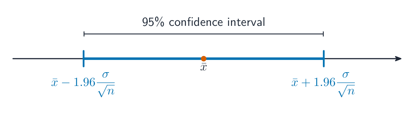
A 95% confidence interval reaches 1.96 standard errors each side of the estimate Choosing the sample size. To keep the margin of error no larger than a target $m$, set $z^{*}\sqrt{\dfrac{\hat p(1-\hat p)}{n}}\le m$ and solve for $n$. When you have no estimate of $\hat p$, use $\hat p=0.5$: it makes $\hat p(1-\hat p)$ as large as possible, giving the safe (largest) required sample size. Always round the result up to the next whole person.
Worked example. How many people must you survey for a $95\%$ interval with margin of error at most $0.03$? Using $\hat p=0.5$ and $z^*=1.96$:
$$n=\frac{(z^*)^2\,\hat p(1-\hat p)}{m^2}=\frac{1.96^2(0.5)(0.5)}{0.03^2}=\frac{0.9604}{0.0009}\approx1067.1,$$so you survey $1068$ people (always round up, since $1067$ would leave the margin a shade too big).Vocabulary TrainEnglish confidence interval/ˈkɒnfɪdəns ˈɪntəvl/ margin of error/ˈmɑːdʒɪn ɒv ˈerə/ confidence level/ˈkɒnfɪdəns ˈlevl/ 6.3
Justifying a Claim from an Interval
Syllabus
Enduring Understanding Learning Objective Essential Knowledge UNC-4
An interval of values should be used to estimate parameters, in order to account for uncertainty.UNC-4.F
Interpret a confidence interval for a population proportion. [Skill 4.B]- UNC-4.F.1 A confidence interval for a population proportion either contains the population proportion or it does not, because each interval is based on random sample data, which varies from sample to sample.
- UNC-4.F.2 We are C% confident that the confidence interval for a population proportion captures the population proportion.
- UNC-4.F.3 In repeated random sampling with the same sample size, approximately C% of confidence intervals created will capture the population proportion.
- UNC-4.F.4 Interpreting a confidence interval for a one-sample proportion should include a reference to the sample taken and details about the population it represents.
- Illustrative examples for UNC-4.F.4: For interpreting a 99% confidence interval of (0.268, 0.292), based on the proportion of a nationally representative sample of twelfth-grade students who answered a particular multiple choice question correctly: "We are 99 percent confident that the interval from 0.268 to 0.292 contains the population proportion of all United States twelfth-grade students who would answer this question correctly" (2011 FRQ 6(a)).
UNC-4.G
Justify a claim based on a confidence interval for a population proportion. [Skill 4.D]- UNC-4.G.1 A confidence interval for a population proportion provides an interval of values that may provide sufficient evidence to support a particular claim in context.
UNC-4.H
Identify the relationships between sample size, width of a confidence interval, confidence level, and margin of error for a population proportion. [Skill 4.A]- UNC-4.H.1 When all other things remain the same, the width of the confidence interval for a population proportion tends to decrease as the sample size increases. For a population proportion, the width of the interval is proportional to $\dfrac{1}{\sqrt{n}}$.
- UNC-4.H.2 For a given sample, the width of the confidence interval for a population proportion increases as the confidence level increases.
- UNC-4.H.3 The width of a confidence interval for a population proportion is exactly twice the margin of error.
Source: College Board AP Course and Exam Description
To judge a claimed value: if it lies inside the interval, the data are consistent with it; if it lies outside, the data give evidence against it. Base the conclusion on whether the plausible values include the claim, in context.
6.4
Setting Up a Test for a Proportion
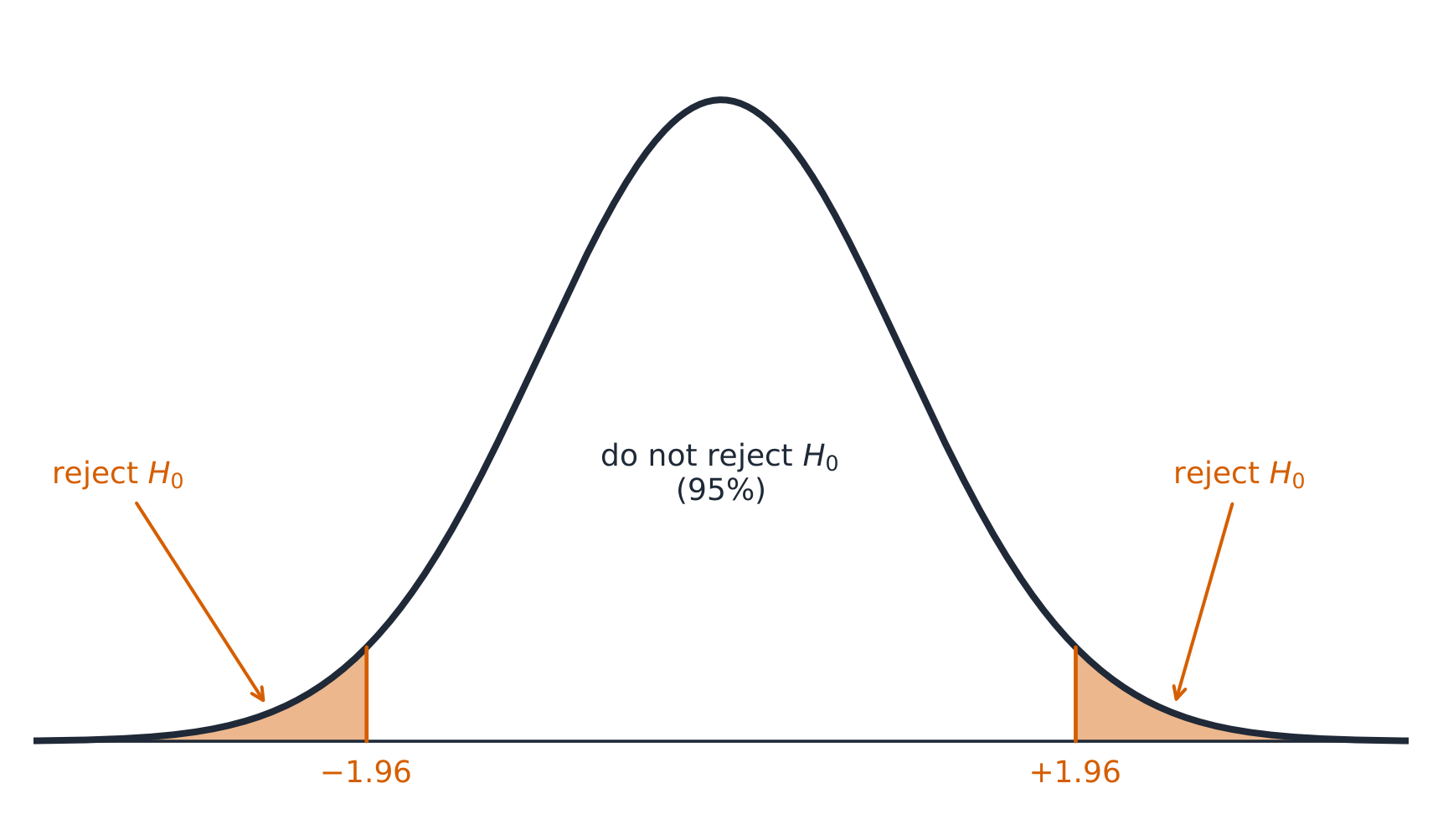
Syllabus
Enduring Understanding Learning Objective Essential Knowledge VAR-6
The normal distribution may be used to model variation.VAR-6.D
Identify the null and alternative hypotheses for a population proportion. [Skill 1.F]- VAR-6.D.1 The null hypothesis is the situation that is assumed to be correct unless evidence suggests otherwise, and the alternative hypothesis is the situation for which evidence is being collected.
- VAR-6.D.2 For hypotheses about parameters, the null hypothesis contains an equality reference (=, ≥, or ≤), while the alternative hypothesis contains a strict inequality (<, >, or ≠). The type of inequality in the alternative hypothesis is based on the question of interest. Alternative hypotheses with < or > are called one-sided, and alternative hypotheses with ≠ are called two-sided. Although the null hypothesis for a one-sided test may include an inequality symbol, it is still tested at the boundary of equality.
- VAR-6.D.3 The null hypothesis for a population proportion is: $H_0 : p = p_0$, where $p_0$ is the null hypothesized value for the population proportion.
- VAR-6.D.4 A one-sided alternative hypothesis for a proportion is either $H_a : p < p_0$ or $H_a : p > p_0$. A two-sided alternate hypothesis is $H_a : p_1 \neq p_2$.
- VAR-6.D.5 For a one-sample $z$-test for a population proportion, the null hypothesis specifies a value for the population proportion, usually one indicating no difference or effect.
VAR-6.E
Identify an appropriate testing method for a population proportion. [Skill 1.E]- VAR-6.E.1 For a single categorical variable, the appropriate testing method for a population proportion is a one-sample $z$-test for a population proportion.
VAR-6.F
Verify the conditions for making statistical inferences when testing a population proportion. [Skill 4.C]- VAR-6.F.1 In order to make statistical inferences when testing a population proportion, we must check for independence and that the sampling distribution is approximately normal:
- a. To check for independence:
- i. Data should be collected using a random sample or a randomized experiment.
- ii. When sampling without replacement, check that $n \leq 10\%N$.
- b. To check that the sampling distribution of $\hat{p}$ is approximately normal (shape):
- i. Assuming that $H_0$ is true $(p = p_0)$, verify that both the number of successes, $np_0$, and the number of failures, $n(1-p_0)$ are at least 10 so that that the sample size is large enough to support an assumption of normality.
- a. To check for independence:
Source: College Board AP Course and Exam Description
A significance test 显著性检验 weighs evidence against a claim. State a null hypothesis 原假设 $H_0$ and an alternative hypothesis 备择假设 $H_a$ about the parameter $p$:
$$H_0: p=p_0 \qquad H_a: p\neq p_0 \ (\text{or } <,\, >).$$Check the same conditions (random, Large Counts using $p_0$, 10%). The test statistic 检验统计量 counts standard errors from $p_0$:$$z=\frac{\hat p-p_0}{\sqrt{p_0(1-p_0)/n}}.$$Worked example. A company claims $90\%$ satisfaction ($p_0=0.90$); a sample of $100$ finds $84$ satisfied ($\hat{p}=0.84$). Test $H_0:p=0.90$ vs $H_a:p\neq0.90$ at $\alpha=0.05$:
$$z=\frac{0.84-0.90}{\sqrt{0.90(0.10)/100}}=\frac{-0.06}{0.03}=-2.0,$$giving a two-tailed $p$-value of about $2(0.023)=0.046$. Since $0.046<0.05$, reject $H_0$ – there is evidence the true satisfaction rate differs from (is below) $90\%$.A two-tailed 5% test rejects the null hypothesis in the shaded tails Vocabulary TrainEnglish significance test/sɪɡˈnɪfɪkəns test/ null hypothesis/nʌl haɪˈpɒθəsɪs/ alternative hypothesis/ɔːlˈtɜːnətɪv haɪˈpɒθəsɪs/ test statistic/test stəˈtɪstɪk/ 6.5
Interpreting p-Values
Syllabus
Enduring Understanding Learning Objective Essential Knowledge VAR-6
The normal distribution may be used to model variation.VAR-6.G
Calculate an appropriate test statistic and $p$-value for a population proportion. [Skill 3.E]- VAR-6.G.1 The distribution of the test statistic assuming the null hypothesis is true (null distribution) can be either a randomization distribution or when a probability model is assumed to be true, a theoretical distribution ($z$).
- VAR-6.G.2 When using a $z$-test, the standardized test statistic can be written: $\text{test statistic} = \dfrac{\text{sample statistic} - \text{null value of the parameter}}{\text{standard deviation of the statistic}}$. This is called a $z$-statistic for proportions.
- VAR-6.G.3 The test statistic for a population proportion is: $z = \dfrac{\hat{p} - p_0}{\sqrt{\dfrac{p_0(1-p_0)}{n}}}$.
- Clarifying statement: The formulas for test statistics do not appear explicitly on the AP Statistics Formula Sheet provided with the AP Statistics Exam. However, these formulas do not need to be memorized, as they can be constructed based on the general test statistic formula and the relevant standard error formulas that are provided on the formula sheet.
- VAR-6.G.4 A $p$-value is the probability of obtaining a test statistic as extreme or more extreme than the observed test statistic when the null hypothesis and probability model are assumed to be true. The significance level may be given or determined by the researcher.
DAT-3
Significance testing allows us to make decisions about hypotheses within a particular context.DAT-3.A
Interpret the $p$-value of a significance test for a population proportion. [Skill 4.B]- DAT-3.A.1 The $p$-value is the proportion of values for the null distribution that are as extreme or more extreme than the observed value of the test statistic. This is:
- a. The proportion at or above the observed value of the test statistic, if the alternative is >.
- b. The proportion at or below the observed value of the test statistic, if the alternative is <.
- c. The proportion less than or equal to the negative of the absolute value of the test statistic plus the proportion greater than or equal to the absolute value of the test statistic, if the alternative is ≠.
- DAT-3.A.2 An interpretation of the $p$-value of a significance test for a one-sample proportion should recognize that the $p$-value is computed by assuming that the probability model and null hypothesis are true, i.e., by assuming that the true population proportion is equal to the particular value stated in the null hypothesis.
Source: College Board AP Course and Exam Description
What a p-value means The $p$-value P值 is the probability of getting a sample result as extreme or more extreme than the observed one, assuming $H_0$ is true. A small $p$-value means the data would be surprising if $H_0$ held – evidence against $H_0$. It is not the probability that $H_0$ is true.
ExploreA p-value as a tail area
A p-value is the probability, if the null hypothesis were true, of a result at least this extreme — the shaded tail area. Small p-values cast doubt on the null.
Vocabulary TrainEnglish p-value/piː ˈvæljuː/ 6.6
Concluding a Test
Syllabus
Enduring Understanding Learning Objective Essential Knowledge DAT-3
Significance testing allows us to make decisions about hypotheses within a particular context.DAT-3.B
Justify a claim about the population based on the results of a significance test for a population proportion. [Skill 4.E]- DAT-3.B.1 The significance level, $\alpha$, is the predetermined probability of rejecting the null hypothesis given that it is true.
- DAT-3.B.2 A formal decision explicitly compares the $p$-value to the significance level, $\alpha$. If the $p$-value $\leq \alpha$, reject the null hypothesis. If the $p$-value $> \alpha$, fail to reject the null hypothesis.
- DAT-3.B.3 Rejecting the null hypothesis means there is sufficient statistical evidence to support the alternative hypothesis. Failing to reject the null means there is insufficient statistical evidence to support the alternative hypothesis.
- DAT-3.B.4 The conclusion about the alternative hypothesis must be stated in context.
- DAT-3.B.5 A significance test can lead to rejecting or not rejecting the null hypothesis, but can never lead to concluding or proving that the null hypothesis is true. Lack of statistical evidence for the alternative hypothesis is not the same as evidence for the null hypothesis.
- DAT-3.B.6 Small $p$-values indicate that the observed value of the test statistic would be unusual if the null hypothesis and probability model were true, and so provide evidence for the alternative. The lower the $p$-value, the more convincing the statistical evidence for the alternative hypothesis.
- DAT-3.B.7 $p$-values that are not small indicate that the observed value of the test statistic would not be unusual if the null hypothesis and probability model were true, so do not provide convincing statistical evidence for the alternative hypothesis nor do they provide evidence that the null hypothesis is true.
- DAT-3.B.8 A formal decision explicitly compares the $p$-value to the significance $\alpha$. If the $p$-value $\leq \alpha$, then reject the null hypothesis, $H_0 : p = p_0$. If the $p$-value $> \alpha$, then fail to reject the null hypothesis.
- DAT-3.B.9 The results of a significance test for a population proportion can serve as the statistical reasoning to support the answer to a research question about the population that was sampled.
Source: College Board AP Course and Exam Description
Compare the $p$-value to the significance level 显著性水平 $\alpha$ (often $0.05$):
- $p\le\alpha$: reject $H_0$ – there is convincing evidence for $H_a$.
- $p>\alpha$: fail to reject $H_0$ – not enough evidence for $H_a$ (never "accept $H_0$").
Always write the conclusion in context, linking back to the claim.
Vocabulary TrainEnglish significance level/sɪɡˈnɪfɪkəns ˈlevl/ 6.7
Type I and Type II Errors
Syllabus
Enduring Understanding Learning Objective Essential Knowledge UNC-5
Probabilities of Type I and Type II errors influence inference.UNC-5.A
Identify Type I and Type II errors. [Skill 1.B]- UNC-5.A.1 A Type I error occurs when the null hypothesis is true and is rejected (false positive).
- UNC-5.A.2 A Type II error occurs when the null hypothesis is false and is not rejected (false negative).
- Table of Errors: With Actual Population Value across the top ($H_0$ true; $H_a$ true) and Decision down the side (Reject $H_0$; Fail to Reject $H_0$): Reject $H_0$ when $H_0$ true = Type I Error; Reject $H_0$ when $H_a$ true = Correct Decision; Fail to Reject $H_0$ when $H_0$ true = Correct Decision; Fail to Reject $H_0$ when $H_a$ true = Type II Error.
UNC-5.B
Calculate the probability of a Type I and Type II errors. [Skill 3.A]- UNC-5.B.1 The significance level, $\alpha$, is the probability of making a Type I error, if the null hypothesis is true.
- UNC-5.B.2 The power of a test is the probability that a test will correctly reject a false null hypothesis.
- UNC-5.B.3 The probability of making a Type II error $= 1 - power$.
UNC-5.C
Identify factors that affect the probability of errors in significance testing. [Skill 4.A]- UNC-5.C.1 The probability of a Type II error decreases when any of the following occurs, provided the others do not change:
- i. Sample size(s) increases.
- ii. Significance level ($\alpha$) of a test increases.
- iii. Standard error decreases.
- iv. True parameter value is farther from the null.
UNC-5.D
Interpret Type I and Type II errors. [Skill 4.B]- UNC-5.D.1 Whether a Type I or a Type II error is more consequential depends upon the situation.
- UNC-5.D.2 Since the significance level, $\alpha$, is the probability of a Type I error, the consequences of a Type I error influence decisions about a significance level.
Source: College Board AP Course and Exam Description
Type I and Type II errors - A Type I error 第一类错误: rejecting a true $H_0$ (a false alarm). Its probability is $\alpha$.
- A Type II error 第二类错误: failing to reject a false $H_0$ (a missed detection). Its probability is $\beta$.
- The power 检验效能 $=1-\beta$ is the chance of correctly detecting a real effect. Power rises with a larger sample, a larger effect, or a larger $\alpha$.
Describe each error and its consequence in the problem's context.
ExploreTwo ways a test can be wrong
A Type I error rejects a true null (false alarm); a Type II error keeps a false null (a miss). Lowering one usually raises the other.
Vocabulary TrainEnglish Type I error/taɪp aɪ ˈerə/ Type II error/taɪp ˈtuː ˈerə/ power/ˈpaʊə/ 6.8
Confidence Interval for a Difference of Proportions
Syllabus
Enduring Understanding Learning Objective Essential Knowledge UNC-4
An interval of values should be used to estimate parameters, in order to account for uncertainty.UNC-4.I
Identify an appropriate confidence interval procedure for a comparison of population proportions. [Skill 1.D]- UNC-4.I.1 The appropriate confidence interval procedure for a two-sample comparison of proportions for one categorical variable is a two-sample $z$-interval for a difference between population proportions.
UNC-4.J
Verify the conditions for calculating confidence intervals for a difference between population proportions. [Skill 4.C]- UNC-4.J.1 In order to calculate confidence intervals to estimate a difference between proportions, we must check for independence and that the sampling distribution is approximately normal:
- a. To check for independence:
- i. Data should be collected using two independent, random samples or a randomized experiment.
- ii. When sampling without replacement, check that $n_1 \leq 10\%N_1$ and $n_2 \leq 10\%N_2$.
- b. To check that sampling distribution of $\hat{p}_1 - \hat{p}_2$ is approximately normal (shape).
- i. For categorical variables, check that $n_1\hat{p}_1$, $n_1(1-\hat{p}_1)$, $n_2\hat{p}_2$, and $n_2\left(1-\hat{p}_2\right)$ are all greater than or equal to some predetermined value, typically either 5 or 10.
- a. To check for independence:
UNC-4.K
Calculate an appropriate confidence interval for a comparison of population proportions. [Skill 3.D]- UNC-4.K.1 For a comparison of proportions, the interval estimate is $(\hat{p}_1 - \hat{p}_2) \pm z^* \sqrt{\dfrac{\hat{p}_1(1-\hat{p}_1)}{n_1} + \dfrac{\hat{p}_2(1-\hat{p}_2)}{n_2}}$.
- Clarifying statement: Formulas for interval estimates do not appear explicitly on the AP Statistics Formula Sheet provided with the AP Statistics Exam. However, these formulas do not need to be memorized, as they can be constructed based on the general test statistic formula and the relevant standard error formulas that are provided on the formula sheet.
UNC-4.L
Calculate an interval estimate based on a confidence interval for a difference of proportions. [Skill 3.D]- UNC-4.L.1 Confidence intervals for a difference in proportions can be used to calculate interval estimates with specified units.
Source: College Board AP Course and Exam Description
To compare two proportions, estimate $p_1-p_2$:
$$(\hat p_1-\hat p_2)\pm z^{*}\sqrt{\frac{\hat p_1(1-\hat p_1)}{n_1}+\frac{\hat p_2(1-\hat p_2)}{n_2}}.$$Conditions must hold in both samples, and the samples must be independent.6.9
Justifying a Claim About Two Proportions
Syllabus
Enduring Understanding Learning Objective Essential Knowledge UNC-4
An interval of values should be used to estimate parameters, in order to account for uncertainty.UNC-4.M
Interpret a confidence interval for a difference of proportions. [Skill 4.B]- UNC-4.M.1 In repeated random sampling with the same sample size, approximately C% of confidence intervals created will capture the difference in population proportions.
- UNC-4.M.2 Interpreting a confidence interval for difference between population proportions should include a reference to the sample taken and details about the population it represents.
UNC-4.N
Justify a claim based on a confidence interval for a difference of proportions. [Skill 4.D]- UNC-4.N.1 A confidence interval for difference in population proportions provides an interval of values that may provide sufficient evidence to support a particular claim in context.
Source: College Board AP Course and Exam Description
If the interval for $p_1-p_2$ contains $0$, the data are consistent with no difference; if it lies entirely above or below $0$, there is evidence of a difference (in that direction). State the direction and context.
6.10
Setting Up a Test for a Difference
Syllabus
Enduring Understanding Learning Objective Essential Knowledge VAR-6
The normal distribution may be used to model variation.VAR-6.H
Identify the null and alternative hypotheses for a difference of two population proportions. [Skill 1.F]- VAR-6.H.1 For a two-sample test for a difference of two proportions, the null hypothesis specifies a value of $0$ for the difference in population proportions, indicating no difference or effect.
- VAR-6.H.2 The null hypothesis for a difference in proportions is: $H_0 : p_1 = p_2$, or $H_0 : p_1 - p_2 = 0$.
- VAR-6.H.3 A one-sided alternative hypothesis for a difference in proportions is $H_a : p_1 < p_2$, or, $H_a : p_1 > p_2$. A two-sided alternative hypothesis for a difference of proportions is $H_a : p_1 \neq p_2$.
VAR-6.I
Identify an appropriate testing method for the difference of two population proportions. [Skill 1.E]- VAR-6.I.1 For a single categorical variable, the appropriate testing method for the difference of two population proportions is a two-sample $z$-test for a difference between two population proportions.
VAR-6.J
Verify the conditions for making statistical inferences when testing a difference of two population proportions. [Skill 4.C]- VAR-6.J.1 In order to make statistical inferences when testing a difference between population proportions, we must check for independence and that the sampling distribution is approximately normal:
- a. To check for independence:
- i. Data should be collected using two independent, random samples or a randomized experiment.
- ii. When sampling without replacement, check that $n_1 \leq 10\%N_1$ and $n_2 \leq 10\%N_2$.
- b. To check that the sampling distribution of $\hat{p}_1 - \hat{p}_2$ is approximately normal (shape):
- i. For the combined sample, define the combined (or pooled) proportion, $\hat{p}_c = \dfrac{n_1\hat{p}_1 + n_2\hat{p}_2}{n_1 + n_2}$. Assuming that $H_0$ is true $(p_1 - p_2 = 0$ or $p_1 = p_2)$, check that $n_1\hat{p}_c$, $n_1\left(1-\hat{p}_c\right)$, $n_2\hat{p}_c$, and $n_2\left(1-\hat{p}_c\right)$ are all greater than or equal to some predetermined value, typically either 5 or 10.
- a. To check for independence:
Source: College Board AP Course and Exam Description
Hypotheses compare the two proportions: $H_0: p_1=p_2$ versus $H_a: p_1\neq p_2$ (or $<,>$). Because $H_0$ says the proportions are equal, use a combined (pooled) 合并 sample proportion $\hat p_c=\dfrac{\text{total successes}}{\text{total sample size}}$ to estimate the common $p$.
Vocabulary TrainEnglish combined (pooled)/kəmˈbaɪnd/ 6.11
Carrying Out a Test for a Difference
Syllabus
Enduring Understanding Learning Objective Essential Knowledge VAR-6
The normal distribution may be used to model variation.VAR-6.K
Calculate an appropriate test statistic for the difference of two population proportions. [Skill 3.E]- VAR-6.K.1 The test statistic for a difference in proportions is: $z = \dfrac{(\hat{p}_1 - \hat{p}_2) - 0}{\sqrt{\hat{p}_c(1-\hat{p}_c)}\sqrt{\dfrac{1}{n_1} + \dfrac{1}{n_2}}}$, where $\hat{p}_c = \dfrac{n_1\hat{p}_1 + n_2\hat{p}_2}{n_1 + n_2}$.
- Clarifying statement: The formulas for test statistics do not appear explicitly on the AP Statistics Formula Sheet provided with the AP Statistics Exam. However, these formulas do not need to be memorized, as they can be constructed based on the general test statistic formula and the standard error formulas for each of the relevant test statistics that are provided on the formula sheet.
DAT-3
Significance testing allows us to make decisions about hypotheses within a particular context.DAT-3.C
Interpret the $p$-value of a significance test for a difference of population proportions. [Skill 4.B]- DAT-3.C.1 An interpretation of the $p$-value of a significance test for a difference of two population proportions should recognize that the $p$-value is computed by assuming that the null hypothesis is true, i.e., by assuming that the true population proportions are equal to each other.
DAT-3.D
Justify a claim about the population based on the results of a significance test for a difference of population proportions. [Skill 4.E]- DAT-3.D.1 A formal decision explicitly compares the $p$-value to the significance $\alpha$. If the $p\text{-value} \leq \alpha$, then reject the null hypothesis, $H_0 : p_1 = p_2$, or $H_0 : p_1 - p_2 = 0$. If the $p$-value $> \alpha$, then fail to reject the null hypothesis.
- DAT-3.D.2 The results of a significance test for a difference of two population proportions can serve as the statistical reasoning to support the answer to a research question about the two populations that were sampled.
Source: College Board AP Course and Exam Description
The pooled two-proportion $z$ statistic:
$$z=\frac{\hat p_1-\hat p_2}{\sqrt{\hat p_c(1-\hat p_c)\left(\frac{1}{n_1}+\frac{1}{n_2}\right)}}.$$Find the $p$-value from the normal model, compare to $\alpha$, and conclude in context – the same four-step logic as the one-proportion test.6.11
Exam tips
- State the conditions (random, 10%, large counts $np,\,nq\ge10$) before any proportion inference.
- A confidence interval = estimate $\pm$ margin of error; "95% confident" refers to the method's long-run capture rate.
- For a test, write $H_0$ and $H_a$, compute the test statistic, find the p-value, and compare to $\alpha$.
- A small p-value is evidence against $H_0$; failing to reject does not prove $H_0$.
- Larger samples shrink the margin of error; a higher confidence level widens it.
-
7
Inference for Quantitative Data: Means
Watch lesson7.1
Should I Worry About Error?
Syllabus
Enduring Understanding Learning Objective Essential Knowledge VAR-1
Given that variation may be random or not, conclusions are uncertain.VAR-1.I
Identify questions suggested by probabilities of errors in statistical inference. [Skill 1.A]- VAR-1.I.1 Random variation may result in errors in statistical inference.
Source: College Board AP Course and Exam Description
Type I and Type II errors Inference for a mean works like inference for a proportion, with one change: we rarely know the population standard deviation $\sigma$, so we estimate it with the sample $s$. That extra uncertainty means we use the $t$-distribution instead of the normal – a distribution 分布 that is bell-shaped but with heavier tails, and it depends on the degrees of freedom 自由度 $df=n-1$; as $n$ grows it approaches the normal.
Vocabulary TrainEnglish distribution/ˌdɪstrɪˈbjuːʃn/ degrees of freedom/dɪˈɡriːz ɒv ˈfriːdəm/ 7.2
Confidence Interval for a Mean
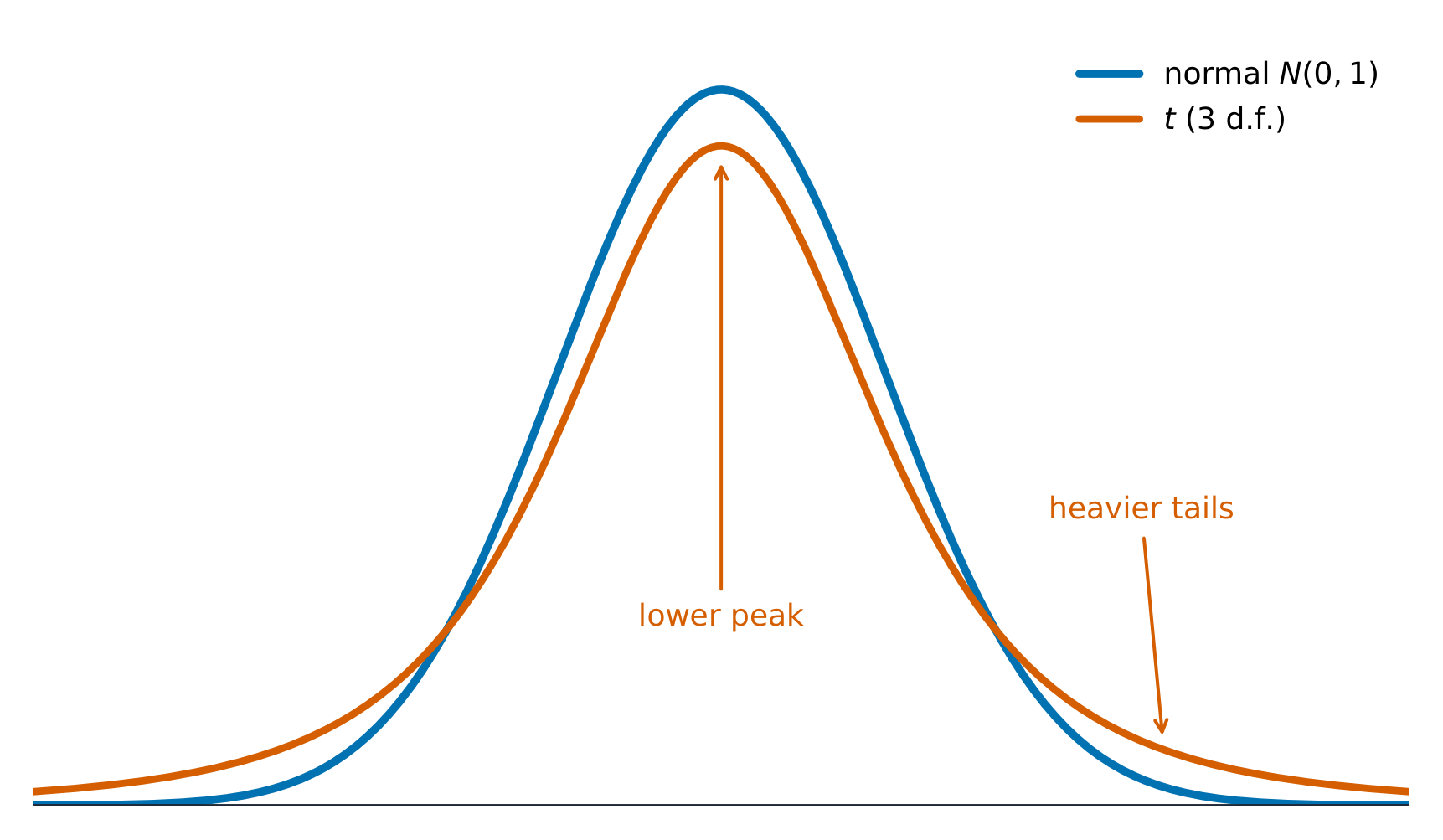
Syllabus
Enduring Understanding Learning Objective Essential Knowledge VAR-7
The $t$-distribution may be used to model variation.VAR-7.A
Describe $t$-distributions. [Skill 3.C]- VAR-7.A.1 When $s$ is used instead of $\sigma$ to calculate a test statistic, the corresponding distribution, known as the $t$-distribution, varies from the normal distribution in shape, in that more of the area is allocated to the tails of the density curve than in a normal distribution.
- VAR-7.A.2 As the degrees of freedom increase, the area in the tails of a $t$-distribution decreases.
UNC-4
An interval of values should be used to estimate parameters, in order to account for uncertainty.UNC-4.O
Identify an appropriate confidence interval procedure for a population mean, including the mean difference between values in matched pairs. [Skill 1.D]- UNC-4.O.1 Because $\sigma$ is typically not known for distributions of quantitative variables, the appropriate confidence interval procedure for estimating the population mean of one quantitative variable for one sample is a one-sample $t$-interval for a mean.
- UNC-4.O.2 For one quantitative variable, $X$, that is normally distributed, the distribution of $t = \dfrac{(\overline{x} - \mu)}{\frac{s}{\sqrt{n}}}$ is a $t$-distribution with $n-1$ degrees of freedom.
- UNC-4.O.3 Matched pairs can be thought of as one sample of pairs. Once differences between pairs of values are found, inference for confidence intervals proceeds as for a population mean.
UNC-4.P
Verify the conditions for calculating confidence intervals for a population mean, including the mean difference between values in matched pairs. [Skill 4.C]- UNC-4.P.1 In order to calculate confidence intervals to estimate a population mean, we must check for independence and that the sampling distribution is approximately normal:
- a. To check for independence:
- i. Data should be collected using a random sample or a randomized experiment.
- ii. When sampling without replacement, check that $n \leq 10\%N$, where $N$ is the size of the population.
- b. To check that the sampling distribution of $\overline{x}$ is approximately normal (shape):
- i. If the observed distribution is skewed, $n$ should be greater than 30.
- ii. If the sample size is less than 30, the distribution of the sample data should be free from strong skewness and outliers.
- a. To check for independence:
UNC-4.Q
Determine the margin of error for a given sample size for a one-sample $t$-interval. [Skill 3.D]- UNC-4.Q.1 The critical value $t^*$ with $n-1$ degrees of freedom can be found using a table or computer-generated output.
- UNC-4.Q.2 The standard error for a sample mean is given by $SE = \dfrac{s}{\sqrt{n}}$, where $s$ is the sample standard deviation.
- UNC-4.Q.3 For a one-sample $t$-interval for a mean, the margin of error is the critical value ($t^*$) times the standard error ($SE$), which equals $t^*\left(\dfrac{s}{\sqrt{n}}\right)$.
UNC-4.R
Calculate an appropriate confidence interval for a population mean, including the mean difference between values in matched pairs. [Skill 3.D]- UNC-4.R.1 The point estimate for a population mean is the sample mean, $\overline{x}$.
- UNC-4.R.2 For the population mean for one sample with unknown population standard deviation, the confidence interval is $\overline{x} \pm t^* \dfrac{s}{\sqrt{n}}$.
Boundary statement: Formulas for interval estimates do not appear explicitly on the AP Statistics Formula Sheet provided with the AP Statistics Exam. However, these formulas do not need to be memorized, as they can be constructed based on the general test statistic formula and the relevant standard error formulas that are provided on the formula sheet.
Source: College Board AP Course and Exam Description
What a confidence interval means A one-sample $t$ interval for $\mu$:
$$\bar{x}\pm t^{*}\frac{s}{\sqrt{n}}.$$$t^{*}$ is the critical value with $df=n-1$. Conditions: random sample, Normal/Large Sample (population normal, or $n\ge 30$ by the CLT, or a roughly symmetric sample with no outliers), and the 10% condition. Interpret the interval and the confidence level in context.Worked example. A random sample of $n=25$ has $\bar{x}=50$ and $s=8$. For a $95\%$ interval, $df=24$ gives $t^*=2.064$:
$$50\pm2.064\cdot\frac{8}{\sqrt{25}}=50\pm2.064(1.6)=50\pm3.3=(46.7,\ 53.3).$$The t-distribution has a lower peak and heavier tails than the normal 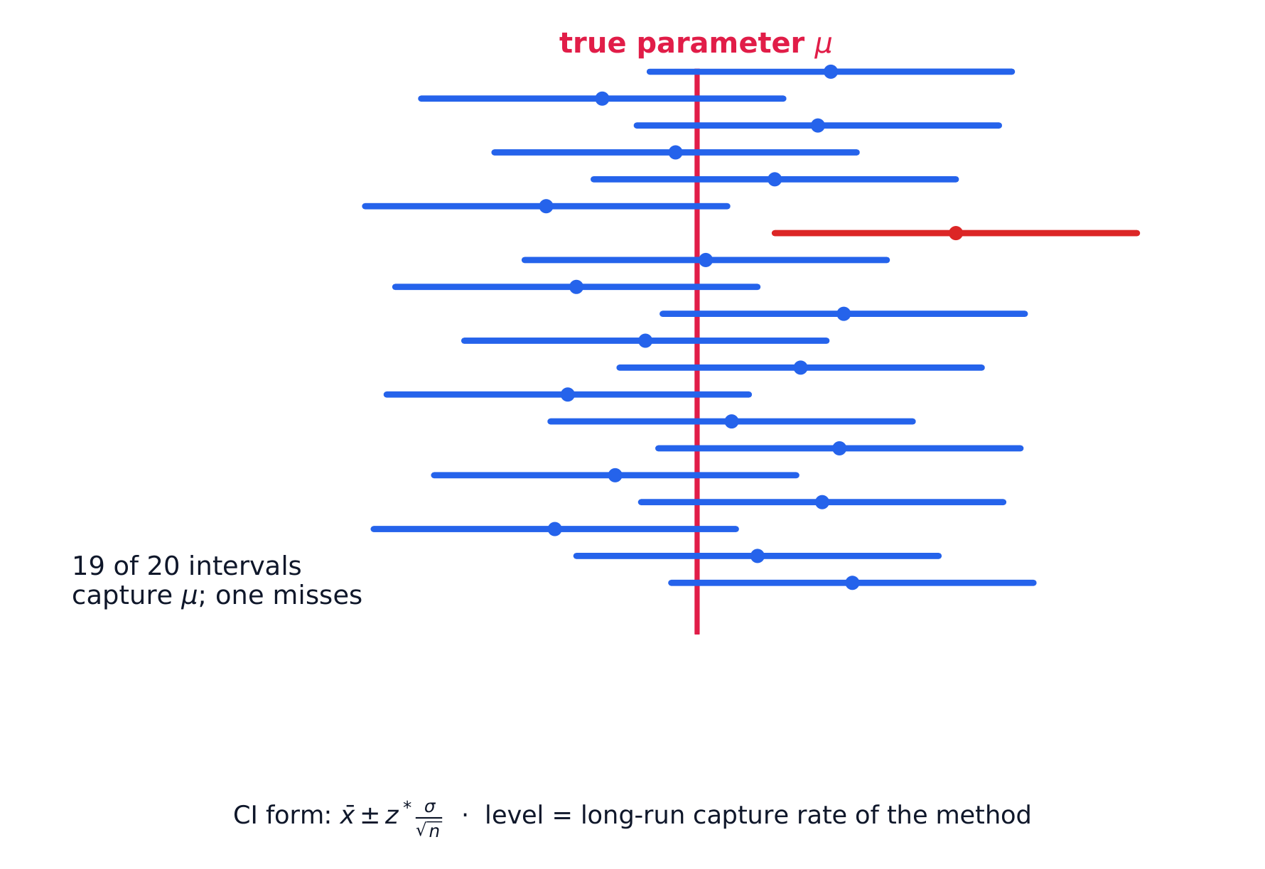
"95% confident" describes the method, not one interval: over many samples about 95% of the intervals contain $\mu$ and about 5% miss it. ExploreWhy a t interval is wider than a z interval
A mean interval uses $t^*$, not $1.96$, because $\sigma$ is estimated by $s$. Drag df down and watch $t^*$ grow — at $df=10$ it is $2.228$, and the interval is wider for it. Drag df up and $t^*$ falls back toward $1.96$, which is why large samples may use $z$.
7.3
Justifying a Claim About a Mean
Syllabus
Enduring Understanding Learning Objective Essential Knowledge UNC-4
An interval of values should be used to estimate parameters, in order to account for uncertainty.UNC-4.S
Interpret a confidence interval for a population mean, including the mean difference between values in matched pairs. [Skill 4.B]- UNC-4.S.1 A confidence interval for a population mean either contains the population mean or it does not, because each interval is based on data from a random sample, which varies from sample to sample.
- UNC-4.S.2 We are C% confident that the confidence interval for a population mean captures the population mean.
- UNC-4.S.3 An interpretation of a confidence interval for a population mean includes a reference to the sample taken and details about the population it represents.
- Illustrative examples for UNC-4.S.3: For interpreting a 96% confidence interval for mean foot length for all footprints found in a cave based on a particular randomly selected sample of footprints in the cave: "We are 96% confident that the mean foot length for all footprints found in the cave falls within the confidence interval" (based on 2000 FRQ 2).
UNC-4.T
Justify a claim based on a confidence interval for a population mean, including the mean difference between values in matched pairs. [Skill 4.D]- UNC-4.T.1 A confidence interval for a population mean provides an interval of values that may provide sufficient evidence to support a particular claim in context.
UNC-4.U
Identify the relationships between sample size, width of a confidence interval, confidence level, and margin of error for a population mean. [Skill 4.A]- UNC-4.U.1 When all other things remain the same, the width of a confidence interval for a population mean tends to decrease as the sample size increases.
- UNC-4.U.2 For a single mean, the width of the interval is proportional to $\dfrac{1}{\sqrt{n}}$.
- UNC-4.U.3 For a given sample, the width of the confidence interval for a population mean increases as the confidence level increases.
Source: College Board AP Course and Exam Description
As with proportions: a claimed mean inside the interval is plausible; outside the interval, the data give evidence against it. Answer in context using the plausible range.
7.4
Setting Up a Test for a Mean
Syllabus
Enduring Understanding Learning Objective Essential Knowledge VAR-7
The $t$-distribution may be used to model variation.VAR-7.B
Identify an appropriate testing method for a population mean with unknown $\sigma$, including the mean difference between values in matched pairs. [Skill 1.E]- VAR-7.B.1 The appropriate test for a population mean with unknown $\sigma$ is a one-sample $t$-test for a population mean.
- VAR-7.B.2 Matched pairs can be thought of as one sample of pairs. Once differences between pairs of values are found, inference for significance testing proceeds as for a population mean.
VAR-7.C
Identify the null and alternative hypotheses for a population mean with unknown $\sigma$, including the mean difference between values in matched pairs. [Skill 1.F]- VAR-7.C.1 The null hypothesis for a one-sample $t$-test for a population mean is $H_0 : \mu = \mu_0$, where $\mu_0$ is the hypothesized value. Depending upon the situation, the alternative hypothesis is $H_a : \mu < \mu_0$, or $H_a : \mu > \mu_0$, or $H_a : \mu \neq \mu_0$.
- VAR-7.C.2 When finding the mean difference, $\mu_d$, between values in a matched pair, it is important to define the order of subtraction.
VAR-7.D
Verify the conditions for the test for a population mean, including the mean difference between values in matched pairs. [Skill 4.C]- VAR-7.D.1 In order to make statistical inferences when testing a population mean, we must check for independence and that the sampling distribution is approximately normal:
- a. To check for independence:
- i. Data should be collected using a random sample or a randomized experiment.
- ii. When sampling without replacement, check that $n \leq 10\%N$.
- b. To check that the sampling distribution of $\overline{x}$ is approximately normal (shape):
- i. If the observed distribution is skewed, $n$ should be greater than 30.
- ii. If the sample size is less than 30, the distribution of the sample data should be free from strong skewness and outliers.
- a. To check for independence:
Source: College Board AP Course and Exam Description
What a p-value means State hypotheses about $\mu$: $H_0:\mu=\mu_0$ versus $H_a:\mu\neq\mu_0$ (or $<,>$). Check the same conditions. The one-sample $t$ statistic:
$$t=\frac{\bar{x}-\mu_0}{s/\sqrt{n}},\qquad df=n-1.$$Worked example. Test $H_0:\mu=45$ against $H_a:\mu\neq45$ for the sample above ($\bar{x}=50$, $s=8$, $n=25$):
$$t=\frac{50-45}{8/\sqrt{25}}=\frac{5}{1.6}=3.13,\qquad df=24.$$This $t$ is far out in the tail (two-tailed $p<0.01$), so reject $H_0$ – strong evidence the mean is not $45$. Notice $45$ also falls outside the $95\%$ interval $(46.7,53.3)$, the same conclusion by two routes.7.5
Carrying Out a Test for a Mean
Syllabus
Enduring Understanding Learning Objective Essential Knowledge VAR-7
The $t$-distribution may be used to model variation.VAR-7.E
Calculate an appropriate test statistic for a population mean, including the mean difference between values in matched pairs. [Skill 3.E]- VAR-7.E.1 For a single quantitative variable when random sampling with replacement from a population that can be modeled with a normal distribution with mean $\mu$ and standard deviation $\sigma$, the sampling distribution of $t = \dfrac{\overline{x} - \mu}{\frac{s}{\sqrt{n}}}$ has a $t$-distribution with $n - 1$ degrees of freedom.
Boundary statement: The formulas for test statistics do not appear explicitly on the AP Statistics Formula Sheet provided with the AP Statistics Exam. However, these formulas do not need to be memorized, as they can be constructed based on the general test statistic formula and the relevant standard error formulas that are provided on the formula sheet.
DAT-3
Significance testing allows us to make decisions about hypotheses within a particular context.DAT-3.E
Interpret the $p$-value of a significance test for a population mean, including the mean difference between values in matched pairs. [Skill 4.B]- DAT-3.E.1 An interpretation of the $p$-value of a significance test for a population mean should recognize that the $p$-value is computed by assuming that the null hypothesis is true, i.e., by assuming that the true population mean is equal to the particular value stated in the null hypothesis.
DAT-3.F
Justify a claim about the population based on the results of a significance test for a population mean. [Skill 4.E]- DAT-3.F.1 A formal decision explicitly compares the $p$-value to the significance $\alpha$. If the $p$-value $\leq \alpha$, then reject the null hypothesis, $H_0 : \mu = \mu_0$. If the $p$-value $> \alpha$, then fail to reject the null hypothesis.
- DAT-3.F.2 The results of a significance test for a population mean can serve as the statistical reasoning to support the answer to a research question about the population that was sampled.
Source: College Board AP Course and Exam Description
Find the $p$-value from the $t$-distribution with $df=n-1$, compare to $\alpha$, and conclude in context – reject or fail to reject $H_0$, then state what that means for the claim. Show the test name, statistic, $df$, and $p$-value.
ExploreRead a p-value off the t curve
The p-value is the shaded tail area beyond your $t$ statistic — both tails for a two-tailed $H_a$. The dashed normal curve behind $t$ shows what you would have got by wrongly using $z$: at small df the $t$ tail is visibly fatter, so the true p-value is larger than the normal would suggest.
7.6
Confidence Interval for a Difference of Two Means

Syllabus
Enduring Understanding Learning Objective Essential Knowledge UNC-4
An interval of values should be used to estimate parameters, in order to account for uncertainty.UNC-4.V
Identify an appropriate confidence interval procedure for a difference of two population means. [Skill 1.D]- UNC-4.V.1 Consider a simple random sample from population 1 of size $n_1$, mean $\mu_1$, and standard deviation $\sigma_1$ and a second simple random sample from population 2 of size $n_2$, mean $\mu_2$, and standard deviation $\sigma_2$. If the distributions of populations 1 and 2 are normal or if both $n_1$ and $n_2$ are greater than 30, then the sampling distribution of the difference of means, $\overline{x}_1 - \overline{x}_2$ is also normal. The mean for the sampling distribution of $\overline{x}_1 - \overline{x}_2$ is $\mu_1 - \mu_2$. The standard deviation of $\overline{x}_1 - \overline{x}_2$ is $\sqrt{\dfrac{(\sigma_1)^2}{n_1} + \dfrac{(\sigma_2)^2}{n_2}}$.
- UNC-4.V.2 The appropriate confidence interval procedure for one quantitative variable for two independent samples is a two-sample $t$-interval for a difference between population means.
UNC-4.W
Verify the conditions to calculate confidence intervals for the difference of two population means. [Skill 4.C]- UNC-4.W.1 In order to calculate confidence intervals to estimate a difference of population means, we must check for independence and that the sampling distribution is approximately normal:
- a. To check for independence:
- i. Data should be collected using two independent, random samples or a randomized experiment.
- ii. When sampling without replacement, check that $n_1 \leq 10\%N_1$ and $n_2 \leq 10\%N_2$.
- b. To check that the sampling distribution of $(\overline{x}_1 - \overline{x}_2)$ should be approximately normal (shape):
- i. If the observed distributions are skewed, both $n_1$ and $n_2$ should be greater than 30.
- a. To check for independence:
UNC-4.X
Determine the margin of error for the difference of two population means. [Skill 3.D]- UNC-4.X.1 For the difference of two sample means, the margin of error is the critical value ($t^*$) times the standard error ($SE$) of the difference of two means.
- UNC-4.X.2 The standard error for the difference in two sample means with sample standard deviations, $s_1$ and $s_2$, is $\sqrt{\dfrac{(s_1)^2}{n_1} + \dfrac{(s_2)^2}{n_2}}$.
UNC-4.Y
Calculate an appropriate confidence interval for a difference of two population means. [Skill 3.D]- UNC-4.Y.1 The point estimate for the difference of two population means is the difference in sample means, $\overline{x}_1 - \overline{x}_2$.
- UNC-4.Y.2 For a difference of two population means where the population standard deviations are not known, the confidence interval is $(\overline{x}_1 - \overline{x}_2) \pm t^* \sqrt{\dfrac{s_1^2}{n_1} + \dfrac{s_2^2}{n_2}}$ where $\pm t^*$ are the critical values for the central C% of a $t$-distribution with appropriate degrees of freedom that can be found using technology.
Boundary statement: Formulas for interval estimates do not appear explicitly on the AP Statistics Formula Sheet provided with the AP Statistics Exam. However, these formulas do not need to be memorized, as they can be constructed based on the general test statistic formula and the relevant standard error formulas that are provided on the formula sheet.
Source: College Board AP Course and Exam Description
For independent samples, estimate $\mu_1-\mu_2$:
$$(\bar{x}_1-\bar{x}_2)\pm t^{*}\sqrt{\frac{s_1^2}{n_1}+\frac{s_2^2}{n_2}}.$$Conditions must hold in both samples. (Use technology for the $df$; do not pool the variances on the AP exam.)Randomisation underpins fair comparison of two groups in a mean difference test 7.7
Justifying a Claim About Two Means
Syllabus
Enduring Understanding Learning Objective Essential Knowledge UNC-4
An interval of values should be used to estimate parameters, in order to account for uncertainty.UNC-4.Z
Interpret a confidence interval for a difference of population means. [Skill 4.B]- UNC-4.Z.1 In repeated random sampling with the same sample size, approximately C% of confidence intervals created will capture the difference of population means.
- UNC-4.Z.2 An interpretation for a confidence interval for the difference of two population means should include a reference to the samples taken and details about the populations they represent.
- Illustrative examples for UNC-4.Z.2: For interpreting a confidence interval for a difference between mean response times for two fire stations (northern - southern): "Based on these samples, one can be 95 percent confident that the difference in the population mean response times (northern - southern) is between -2.37 minutes and 0.37 minutes" (2009 FRQ 4).
UNC-4.AA
Justify a claim based on a confidence interval for a difference of population means. [Skill 4.D]- UNC-4.AA.1 A confidence interval for a difference of population means provides an interval of values that may provide sufficient evidence to support a particular claim in context.
UNC-4.AB
Identify the effects of sample size on the width of a confidence interval for the difference of two means. [Skill 4.A]- UNC-4.AB.1 When all other things remain the same, the width of the confidence interval for the difference of two means tends to decrease as the sample sizes increase.
Source: College Board AP Course and Exam Description
If the interval for $\mu_1-\mu_2$ contains $0$, the data are consistent with equal means; if it excludes $0$, there is evidence of a difference in that direction. Interpret in context.
7.8
Setting Up a Test for a Difference of Means
Syllabus
Enduring Understanding Learning Objective Essential Knowledge VAR-7
The $t$-distribution may be used to model variation.VAR-7.F
Identify an appropriate selection of a testing method for a difference of two population means. [Skill 1.E]- VAR-7.F.1 For a quantitative variable, the appropriate test for a difference of two population means is a two-sample $t$-test for a difference of two population means.
VAR-7.G
Identify the null and alternative hypotheses for a difference of two population means. [Skill 1.F]- VAR-7.G.1 The null hypothesis for a two-sample $t$-test for a difference of two population means, $\mu_1$ and $\mu_2$, is: $H_0 : \mu_1 - \mu_2 = 0$, or $H_0 : \mu_1 = \mu_2$. The alternative hypothesis is $H_a : \mu_1 - \mu_2 < 0$, or $H_a : \mu_1 - \mu_2 > 0$, or $H_a : \mu_1 - \mu_2 \neq 0$, or $H_a : \mu_1 > \mu_2$, or $H_a : \mu_1 < \mu_2$, or $H_a : \mu_1 \neq \mu_2$.
VAR-7.H
Verify the conditions for the significance test for the difference of two population means. [Skill 4.C]- VAR-7.H.1 In order to make statistical inferences when testing a difference between population means, we must check for independence and that the sampling distribution is approximately normal:
- a. Individual observations should be independent:
- i. Data should be collected using simple random samples or a randomized experiment.
- ii. When sampling without replacement, check that $n_1 \leq 10\%N_1$ and $n_2 \leq 10\%N_2$.
- b. The sampling distribution of $\overline{x}_1 - \overline{x}_2$ should be approximately normal (shape).
- i. If the observed distribution is skewed, both $n_1$ and $n_2$ should be greater than 30.
- ii. If the sample size is less than 30, the distribution of the sample data should be free from strong skewness and outliers. This should be checked for BOTH samples.
- a. Individual observations should be independent:
Source: College Board AP Course and Exam Description
Hypotheses: $H_0:\mu_1=\mu_2$ versus $H_a:\mu_1\neq\mu_2$ (or $<,>$). Distinguish two independent samples from paired data 配对数据 – for paired data (before/after, matched subjects), first take the differences and run a one-sample $t$ procedure on them.
Vocabulary TrainEnglish paired data/peəd ˈdeɪtə/ 7.9
Carrying Out a Test for a Difference of Means
Syllabus
Enduring Understanding Learning Objective Essential Knowledge VAR-7
The $t$-distribution may be used to model variation.VAR-7.I
Calculate an appropriate test statistic for a difference of two means. [Skill 3.E]- VAR-7.I.1 For a single quantitative variable, data collected using independent random samples or a randomized experiment from two populations, each of which can be modeled with a normal distribution, the sampling distribution of $t = \dfrac{(\overline{x}_1 - \overline{x}_2) - (\mu_1 - \mu_2)}{\sqrt{\dfrac{s_1^2}{n_1} + \dfrac{s_2^2}{n_2}}}$ is an approximate $t$-distribution with degrees of freedom that can be found using technology. The degrees of freedom fall between the smaller of $n_1 - 1$ and $n_2 - 1$ and $n_1 + n_2 - 2$.
- Illustrative examples for VAR-7.I.1: In a study comparing mean recovery times for two surgical procedures to repair a torn anterior cruciate ligament (ACL), the group receiving one procedure had a sample size of 110, while the group receiving the other procedure had a sample size of 100. The degrees of freedom fall between 100 (the smaller of 110 and 100) and 208 (110 + 100 - 2). The degrees of freedom may be determined using technology. If the test statistic for this study is $t \approx 7.13$, then the $p$-value is the area greater than 7.13 for a $t$-distribution with $df = 207.18$ (2018 FRQ 4).
Boundary statement: The formulas for test statistics do not appear explicitly on the AP Statistics Formula Sheet provided with the AP Statistics Exam. However, these formulas do not need to be memorized, as they can be constructed based on the general test statistic formula and the standard error formulas for each of the relevant test statistics that are provided on the formula sheet.
DAT-3
Significance testing allows us to make decisions about hypotheses within a particular context.DAT-3.G
Interpret the $p$-value of a significance test for a difference of population means. [Skill 4.B]- DAT-3.G.1 An interpretation of the $p$-value of a significance test for a two-sample difference of population means should recognize that the $p$-value is computed by assuming that the null hypothesis is true, i.e., by assuming that the true population means are equal to each other.
DAT-3.H
Justify a claim about the population based on the results of a significance test for a difference of two population means in context. [Skill 4.E]- DAT-3.H.1 A formal decision explicitly compares the $p$-value to the significance $\alpha$. If the $p$-value $\leq \alpha$, then reject the null hypothesis, $H_0 : \mu_1 - \mu_2 = 0$, or $H_0 : \mu_1 = \mu_2$. If the $p$-value $> \alpha$, then fail to reject the null hypothesis.
- DAT-3.H.2 The results of a significance test for a two-sample test for a difference between two population means can serve as the statistical reasoning to support the answer to a research question about the populations that were sampled.
Source: College Board AP Course and Exam Description
The two-sample $t$ statistic:
$$t=\frac{(\bar{x}_1-\bar{x}_2)-0}{\sqrt{\frac{s_1^2}{n_1}+\frac{s_2^2}{n_2}}}.$$Get the $p$-value (technology for $df$), compare to $\alpha$, conclude in context.7.10
Selecting and Communicating a Procedure
Syllabus
This topic is intended to focus on the skill of selecting an appropriate inference procedure, now that students have a range of options. Students should be given opportunities to practice when and how to apply all learning objectives relating to inference involving proportions or means.
Source: College Board AP Course and Exam Description
The hardest exam skill is choosing the right procedure: one or two samples? proportion or mean? paired or independent? confidence interval or test? Read the question for what is being estimated or claimed, then name the procedure, check its conditions, carry it out, and communicate the conclusion clearly with numbers and context.
7.10
Exam tips
- Use t-procedures for means (population $\sigma$ unknown) — the t-distribution has heavier tails than normal.
- Check conditions: random, independent, and roughly normal (or large $n$).
- Interpret an interval and a test in context, always tied to the parameter (the true mean).
- Match the right procedure: one-sample, two-sample, or paired (look for a natural pairing).
- State the degrees of freedom; for a two-sample $t$-test use technology's value (or, by hand, the conservative smaller $n-1$).
-
8
Inference for Categorical Data: Chi-Square
Watch lesson8.1
Are My Results Unexpected?
Syllabus
Enduring Understanding Learning Objective Essential Knowledge VAR-1
Given that variation may be random or not, conclusions are uncertain.VAR-1.J
Identify questions suggested by variation between observed and expected counts in categorical data. [Skill 1.A]- VAR-1.J.1 Variation between what we find and what we expect to find may be random or not.
Source: College Board AP Course and Exam Description
When data are counts spread across several categories, we test whether the observed counts differ from what a claim predicts. The tool is the chi-square 卡方 ($\chi^2$) statistic, which adds up the standardized gaps between observed and expected counts:
$$\chi^2=\sum \frac{(\text{observed}-\text{expected})^2}{\text{expected}}.$$A large $\chi^2$ means the observed counts are far from expected – evidence against the claim. The chi-square distribution is right-skewed and depends on its degrees of freedom 自由度.Vocabulary TrainEnglish chi-square/kaɪ skweə/ degrees of freedom/dɪˈɡriːz ɒv ˈfriːdəm/ 8.2
Setting Up a Goodness-of-Fit Test
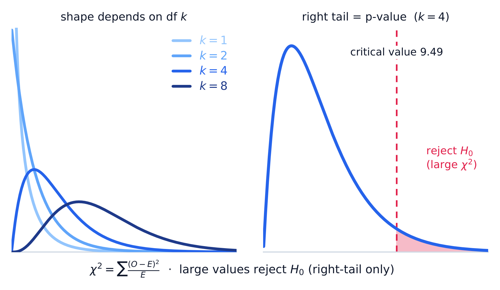
Syllabus
Enduring Understanding Learning Objective Essential Knowledge VAR-8
The chi-square distribution may be used to model variation.VAR-8.A
Describe chi-square distributions. [Skill 3.C]-
VAR-8.A.1 Expected counts of categorical data are counts consistent with the null hypothesis. In general, an expected count is a sample size times a probability.
The chi-square statistic measures the distance between observed and expected counts relative to expected counts.
Chi-square distributions have positive values and are skewed right. Within a family of density curves, the skew becomes less pronounced with increasing degrees of freedom.
VAR-8.B
Identify the null and alternative hypotheses in a test for a distribution of proportions in a set of categorical data. [Skill 1.F]- VAR-8.B.1 For a chi-square goodness-of-fit test, the null hypothesis specifies null proportions for each category, and the alternative hypothesis is that at least one of these proportions is not as specified in the null hypothesis.
VAR-8.C
Identify an appropriate testing method for a distribution of proportions in a set of categorical data. [Skill 1.E]- VAR-8.C.1 When considering a distribution of proportions for one categorical variable, the appropriate test is the chi-square test for goodness of fit.
VAR-8.D
Calculate expected counts for the chi-square test for goodness of fit. [Skill 3.A]- VAR-8.D.1 Expected counts for a chi-square goodness-of-fit test are (sample size)(null proportion).
VAR-8.E
Verify the conditions for making statistical inferences when testing goodness of fit for a chi-square distribution. [Skill 4.C]- VAR-8.E.1 In order to make statistical inferences for a chi-square test for goodness of fit we must check the following:
- a. To check for independence:
- i. Data should be collected using a random sample or randomized experiment.
- ii. When sampling without replacement, check that $n \leq 10\%N$.
- b. The chi-square test for goodness of fit becomes more accurate with more observations, so large counts should be used (shape).
- i. A conservative check for large counts is that all expected counts should be greater than 5.
- a. To check for independence:
Source: College Board AP Course and Exam Description
The chi-square (χ²) test A goodness-of-fit (GOF) 拟合优度 test checks whether one categorical variable follows a claimed distribution (e.g. "the die is fair"). Hypotheses:
$$H_0:\text{the distribution is as claimed}\qquad H_a:\text{at least one proportion differs}.$$Expected count for each category $=n\times(\text{claimed proportion})$. Conditions: random sample, all expected counts $\ge 5$, and the 10% condition.The chi-square distribution is right-skewed. A large statistic lands in the shaded right tail past the critical value – that is where you reject the model. Vocabulary TrainEnglish goodness-of-fit (GOF)/ˈɡʊdnəs ɒv fɪt/ 8.3
Carrying Out a Goodness-of-Fit Test
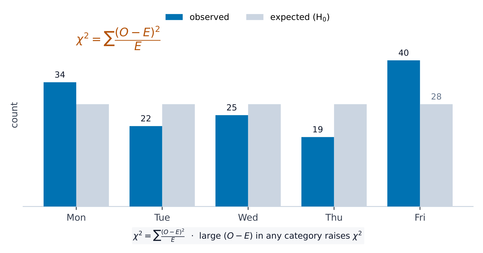
Syllabus
Enduring Understanding Learning Objective Essential Knowledge VAR-8
The chi-square distribution may be used to model variation.VAR-8.F
Calculate the appropriate statistic for the chi-square test for goodness of fit. [Skill 3.E]- VAR-8.F.1 The test statistic for the chi-square test for goodness of fit is
- Equation: $\chi^2 = \sum \dfrac{(Observed\ count - Expected\ count)^2}{Expected\ count}$, with $degrees\ of\ freedom = number\ of\ categories - 1$.
- VAR-8.F.2 The distribution of the test statistic assuming the null hypothesis is true (null distribution) can be either a randomization distribution or, when a probability model is assumed to be true, a theoretical distribution (chi-square).
VAR-8.G
Determine the $p$-value for chi-square test for goodness of fit significance test. [Skill 3.E]- VAR-8.G.1 The $p$-value for a chi-square test for goodness of fit for a number of degrees of freedom is found using the appropriate table or computer generated output.
DAT-3
Significance testing allows us to make decisions about hypotheses within a particular context.DAT-3.I
Interpret the $p$-value for the chi-square test for goodness of fit. [Skill 4.B]- DAT-3.I.1 An interpretation of the $p$-value for the chi-square test for goodness of fit is the probability, given the null hypothesis and probability model are true, of obtaining a test statistic as, or more, extreme than the observed value.
DAT-3.J
Justify a claim about the population based on the results of a chi-square test for goodness of fit. [Skill 4.E]- DAT-3.J.1 A decision to either reject or fail to reject the null hypothesis is based on comparison of the $p$-value to the significance level, $\alpha$.
- DAT-3.J.2 The results of a chi-square test for goodness of fit can serve as the statistical reasoning to support the answer to a research question about the population that was sampled.
Source: College Board AP Course and Exam Description
Compute $\chi^2=\sum\dfrac{(O-E)^2}{E}$ with $df=(\text{number of categories})-1$. Find the $p$-value from the chi-square distribution (upper tail), compare to $\alpha$, and conclude in context. A large component of the sum points to the category that deviates most.
Chi-square compares observed counts with those expected under the null hypothesis Worked example. A die rolled $60$ times gives counts $8,10,12,9,11,10$. If it is fair, each expected count is $60/6=10$, so
$$\chi^2=\frac{(8-10)^2}{10}+\frac{(10-10)^2}{10}+\frac{(12-10)^2}{10}+\frac{(9-10)^2}{10}+\frac{(11-10)^2}{10}+\frac{(10-10)^2}{10}=0.4+0+0.4+0.1+0.1+0=1.0,$$with $df=6-1=5$. Write out every category, including the two that match their expected count exactly and so add $0$ – the sum runs over all six categories, and $df$ counts categories, not just the ones that differ. This $\chi^2$ is small (a large $p$-value), so we fail to reject $H_0$ – no evidence the die is unfair.ExploreExplore the chi-square distribution and its p-value
The p-value is the area in the right tail beyond your test statistic, so a larger $\chi^2$ means a smaller p-value. Drag $\chi^2$ to watch that area shrink, and drag df to see the whole family change shape — strongly right-skewed at small df, more symmetric as df grows.
8.4
Expected Counts in Two-Way Tables
Syllabus
Enduring Understanding Learning Objective Essential Knowledge VAR-8
The chi-square distribution may be used to model variation.VAR-8.H
Calculate expected counts for two-way tables of categorical data. [Skill 3.A]- VAR-8.H.1 The expected count in a particular cell of a two-way table of categorical data can be calculated using the formula:
- Equation: $expected\ count = \dfrac{(row\ total)(column\ total)}{table\ total}$.
Source: College Board AP Course and Exam Description
For a two-way table, the expected count in a cell (under "no association") is
$$E=\frac{(\text{row total})\times(\text{column total})}{\text{grand total}}.$$This is the count you would see if the row and column variables were unrelated.Worked example. In a two-way table a cell's row total is $40$, its column total is $50$, and the grand total is $200$. Its expected count is $E=\dfrac{40\times50}{200}=10$. Repeating for every cell gives the expected table to compare against the observed one.
A spreadsheet organises categorical counts before a chi-square test 8.5
Homogeneity or Independence?
Syllabus
Enduring Understanding Learning Objective Essential Knowledge VAR-8
The chi-square distribution may be used to model variation.VAR-8.I
Identify the null and alternative hypotheses for a chi-square test for homogeneity or independence. [Skill 1.F]-
VAR-8.I.1 The appropriate hypotheses for a chi-square test for homogeneity are:
$H_0$: There is no difference in distributions of a categorical variable across populations or treatments.
$H_a$: There is a difference in distributions of a categorical variable across populations or treatments.
-
VAR-8.I.2 The appropriate hypotheses for a chi-square test for independence are:
$H_0$: There is no association between two categorical variables in a given population or the two categorical variables are independent.
$H_a$: Two categorical variables in a population are associated or dependent.
VAR-8.J
Identify an appropriate testing method for comparing distributions in two-way tables of categorical data. [Skill 1.E]- VAR-8.J.1 When comparing distributions to determine whether proportions in each category for categorical data collected from different populations are the same, the appropriate test is the chi-square test for homogeneity.
- VAR-8.J.2 To determine whether row and column variables in a two-way table of categorical data might be associated in the population from which the data were sampled, the appropriate test is the chi-square test for independence.
VAR-8.K
Verify the conditions for making statistical inferences when testing a chi-square distribution for independence or homogeneity. [Skill 4.C]- VAR-8.K.1 In order to make statistical inferences for a chi-square test for two-way tables (homogeneity or independence), we must verify the following:
- a. To check for independence:
- i. For a test for independence: Data should be collected using a simple random sample.
- ii. For a test for homogeneity: Data should be collected using a stratified random sample or randomized experiment.
- iii. When sampling without replacement, check that $n \leq 10\%N$.
- b. The chi-square tests for independence and homogeneity become more accurate with more observations, so large counts should be used (shape).
- i. A conservative check for large counts is that all expected counts should be greater than 5.
- a. To check for independence:
Source: College Board AP Course and Exam Description
Two tests use the same $\chi^2$ math but answer different questions:
- Test for homogeneity 同质性: are the distributions of one categorical variable the same across several populations or groups (separate samples/treatments)?
- Test for independence 独立性: are two categorical variables associated within a single population (one sample, two variables measured)?
The design (several samples vs one sample) decides which name and hypotheses to use.
Vocabulary TrainEnglish Test for homogeneity/test fɔː ˈhɒməʊdʒneɪti/ Test for independence/test fɔː ˌɪndɪˈpendəns/ 8.6
Carrying Out a Test for Homogeneity or Independence
Syllabus
Enduring Understanding Learning Objective Essential Knowledge VAR-8
The chi-square distribution may be used to model variation.VAR-8.L
Calculate the appropriate statistic for a chi-square test for homogeneity or independence. [Skill 3.E]- VAR-8.L.1 The appropriate test statistic for a chi-square test for homogeneity or independence is the chi-square statistic:
- Equation: $\chi^2 = \sum \dfrac{(Observed\ count - Expected\ count)^2}{Expected\ count}$, with degrees of freedom equal to: $(number\ of\ rows - 1)(number\ of\ columns - 1)$.
VAR-8.M
Determine the $p$-value for a chi-square significance test for independence or homogeneity. [Skill 3.E]- VAR-8.M.1 The $p$-value for a chi-square test for independence or homogeneity for a number of degrees of freedom is found using the appropriate table or technology.
- VAR-8.M.2 For a test of independence or homogeneity for a two-way table, the $p$-value is the proportion of values in a chi-square distribution with appropriate degrees of freedom that are equal to or larger than the test statistic.
DAT-3
Significance testing allows us to make decisions about hypotheses within a particular context.DAT-3.K
Interpret the $p$-value for the chi-square test for homogeneity or independence. [Skill 4.B]- DAT-3.K.1 An interpretation of the $p$-value for the chi-square test for homogeneity or independence is the probability, given the null hypothesis and probability model are true, of obtaining a test statistic as, or more, extreme than the observed value.
DAT-3.L
Justify a claim about the population based on the results of a chi-square test for homogeneity or independence. [Skill 4.E]- DAT-3.L.1 A decision to either reject or fail to reject the null hypothesis for a chi-square test for homogeneity or independence is based on comparison of the $p$-value to the significance level, $\alpha$.
- DAT-3.L.2 The results of a chi-square test for homogeneity or independence can serve as the statistical reasoning to support the answer to a research question about the population that was sampled (independence) or the populations that were sampled (homogeneity).
Source: College Board AP Course and Exam Description
Compute expected counts, then $\chi^2=\sum\dfrac{(O-E)^2}{E}$ over all cells, with
$$df=(\text{rows}-1)(\text{columns}-1).$$Conditions: random data, all expected counts $\ge 5$, 10% condition. Find the $p$-value, compare to $\alpha$, and conclude in context – evidence of a difference between groups (homogeneity) or of an association (independence).8.7
Choosing the Right Categorical Procedure
Syllabus
This topic is intended to focus on the skill of selecting an appropriate inference procedure now that students have a range of options. Students should be given opportunities to practice when and how to apply all learning objectives relating to inference for categorical data.
Source: College Board AP Course and Exam Description
Decide by the setup: one categorical variable against a claimed distribution $\Rightarrow$ goodness-of-fit; one sample cross-classified by two variables $\Rightarrow$ independence; several samples/groups compared $\Rightarrow$ homogeneity. Comparing just two proportions can use either a two-proportion $z$-test or a chi-square test, but only for a two-tailed alternative, where they agree exactly ($\chi^2=z^2$). A chi-square test is always two-tailed, so it cannot give a directional conclusion: if $H_a$ is one-tailed (say $p_1>p_2$), use the $z$-test.
ExploreWhich chi-square test is this?
All three tests use the same $\chi^2$ arithmetic, so the marks are won by naming the right one. The design decides — how many samples were taken, and how many variables were measured on each unit.
8.7
Exam tips
- Use $\chi^2=\sum\tfrac{(O-E)^2}{E}$ for categorical data; always divide by the expected count.
- Pick the right test: goodness-of-fit (one variable), independence, or homogeneity (two-way table).
- Compute expected counts as $\tfrac{\text{row total}\times\text{column total}}{\text{grand total}}$ and check each is $\ge5$.
- A large $\chi^2$ (small p-value) means observed counts differ from expected by more than chance.
- State degrees of freedom correctly (categories $-1$, or $(r-1)(c-1)$).
-
9
Inference for Quantitative Data: Slopes
Watch lesson9.1
Do Those Points Align?
Syllabus
Enduring Understanding Learning Objective Essential Knowledge VAR-1
Given that variation may be random or not, conclusions are uncertain.VAR-1.K
Identify questions suggested by variation in scatter plots. [Skill 1.A]- VAR-1.K.1 Variation in points' positions relative to a theoretical line may be random or non-random.
Source: College Board AP Course and Exam Description
A sample scatterplot 散点图 gives a sample slope 样本斜率 $b$ for the least-squares regression 回归 line – but a different sample would give a slightly different slope. So $b$ is a statistic with sampling variability 抽样变异性, estimating the true (population) slope 总体斜率 $\beta$. This unit does inference 推断 for $\beta$: is there a real linear 线性 relationship, and how strong is it?
Vocabulary TrainEnglish scatterplot/ˈskætəplɒt/ sample slope/ˈsæmpl sləʊp/ regression/rɪˈɡreʃn/ sampling variability/ˈsæmplɪŋ ˌveərɪəˈbɪlɪti/ true (population) slope/truː sləʊp/ inference/ˈɪnfərəns/ linear/ˈlɪnɪə/ 9.2
Confidence Interval for a Slope
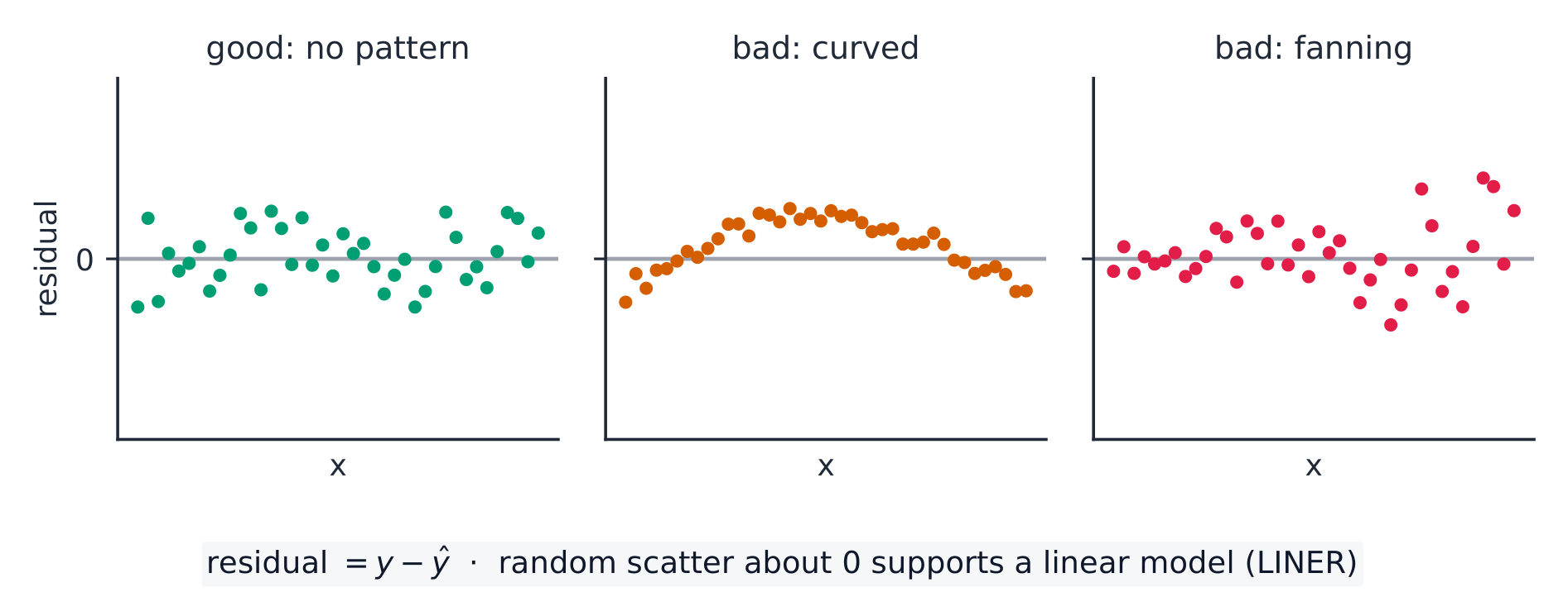
Syllabus
Enduring Understanding Learning Objective Essential Knowledge UNC-4
An interval of values should be used to estimate parameters, in order to account for uncertainty.UNC-4.AC
Identify an appropriate confidence interval procedure for a slope of a regression model. [Skill 1.D]- UNC-4.AC.1 Consider a response variable, $y$, that is linearly related to an explanatory variable, $x$. For a simple random sample of $n$ observations, the sample regression line, $\hat{y} = a + bx$, is an estimate of the population regression line $\mu_y = \alpha + \beta x$. For a particular observation, $(x_i, y_i)$, the residual from the sample regression line, $y_i - \hat{y}_i = y_i - (a + bx_i)$, is an estimate of $y_i - (\alpha + \beta x_i)$, the deviation of the response variable from the population regression line. For all points $(x, y)$ in the population, the standard deviation of all of the deviations of the response variable from the population regression line, $\sigma$, can be estimated by the standard deviation of the residuals from the sample regression line, $s = \sqrt{\dfrac{\sum\left(y_i - \hat{y}_i\right)^2}{n-2}}$. (Note: This formula uses $n-2$ in the denominator instead of $n-1$ because two parameters, $\alpha$ and $\beta$, must be estimated to obtain the predicted values from the least-squares regression line.)
- UNC-4.AC.2 For a simple random sample of $n$ observations, let $b$ represent the slope of a sample regression line. Then the mean of the sampling distribution for $b$ equals the population slope: $\mu_b = \beta$. The standard deviation of the sampling distribution for $b$ is $\sigma_b = \dfrac{\sigma}{\sigma_x \sqrt{n}}$, where $\sigma_x = \sqrt{\dfrac{\sum\left(x_i - \bar{x}\right)^2}{n}}$.
- UNC-4.AC.3 The appropriate confidence interval for the slope of a regression model is a $t$-interval for the slope.
UNC-4.AD
Verify the conditions to calculate confidence intervals for the slope of a regression model. [Skill 4.C]- UNC-4.AD.1 In order to calculate a confidence interval to estimate the slope of a regression line, we must check the following:
- a. The true relationship between $x$ and $y$ is linear. Analysis of residuals may be used to verify linearity.
- b. The standard deviation for $y$, $\sigma_y$, does not vary with $x$. Analysis of residuals may be used to check for approximately equal standard deviations for all $x$.
- c. To check for independence:
- i. Data should be collected using a random sample or a randomized experiment.
- ii. When sampling without replacement, check that $n \le 10\% N$.
- d. For a particular value of $x$, the responses ($y$-values) are approximately normally distributed. Analysis of graphical representations of residuals may be used to check for normality.
- i. If the observed distribution is skewed, $n$ should be greater than 30.
UNC-4.AE
Determine the given margin of error for the slope of a regression model. [Skill 3.D]- UNC-4.AE.1 For the slope of a regression line, the margin of error is the critical value $\left(t^*\right)$ times the standard error ($SE$) of the slope.
- UNC-4.AE.2 The standard error for the slope of a regression line with sample standard deviation, $s$, is $SE = \dfrac{s}{s_x \sqrt{n-1}}$, where $s$ is the estimate of $\sigma$ and $s_x$ is the sample standard deviation of the $x$ values.
UNC-4.AF
Calculate an appropriate confidence interval for the slope of a regression model. [Skill 3.D]- UNC-4.AF.1 The point estimate for the slope of a regression model is the slope of the line of best fit, $b$.
- UNC-4.AF.2 For the slope of a regression model, the interval estimate is $b \pm t^* \left(SE_b\right)$.
Source: College Board AP Course and Exam Description
A $t$ interval for the true slope $\beta$:
$$b\pm t^{*}\,SE_b,\qquad df=n-2,$$where $b$ is the sample slope and $SE_b$ its standard error (read from computer output). Conditions (LINER): the true relationship is Linear, observations Independent, residuals Normal, and residuals have Equal spread (check the residual plot and a histogram of residuals), from Random data. Interpret the interval for $\beta$ in context, with units of $y$ per unit of $x$.A random, patternless residual plot supports the conditions; a curve or a fan does not The residual plot 残差图 is where you check Linear and Equal-spread: you want a formless cloud around zero. A curve means the relationship is not linear; a fan (spread growing with $x$) means the residuals do not have equal spread – both break a condition.
Worked example. Regression output gives slope $b=2.5$ with $SE_b=0.8$ from $n=20$ points. For a $95\%$ interval, $df=18$ gives $t^*=2.101$:
$$2.5\pm2.101(0.8)=2.5\pm1.68=(0.82,\ 4.18).$$Because $0$ is not in the interval, there is evidence of a positive linear relationship.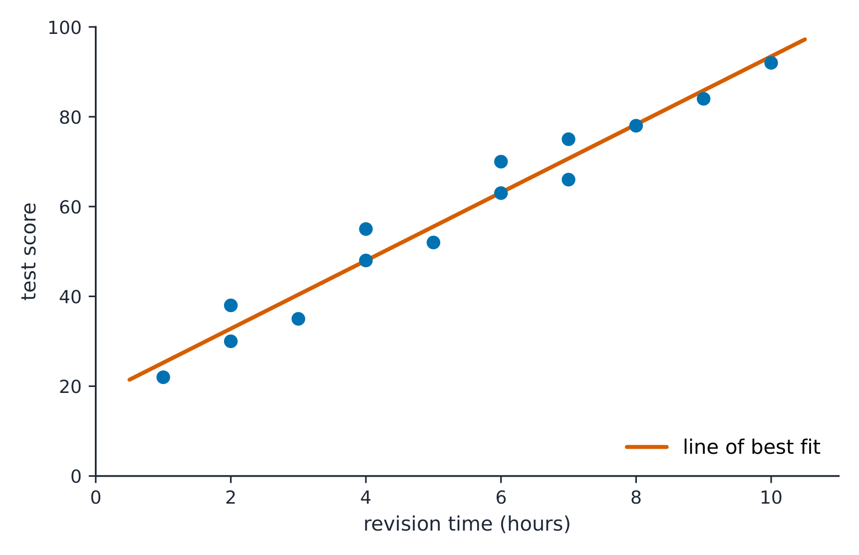
Slope inference is based on the least-squares regression line through the points 
Least-squares regression: the line that minimises the sum of squared residuals ExploreInference for a regression slope
The sample slope varies from sample to sample; a confidence interval and t-test ask whether the true slope could be zero (no linear relationship).
Vocabulary TrainEnglish residual plot/rɪˈsɪdʒuːəl plɒt/ 9.3
Justifying a Claim About a Slope
Syllabus
Enduring Understanding Learning Objective Essential Knowledge UNC-4
An interval of values should be used to estimate parameters, in order to account for uncertainty.UNC-4.AG
Interpret a confidence interval for the slope of a regression model. [Skill 4.B]- UNC-4.AG.1 In repeated random sampling with the same sample size, approximately C% of confidence intervals created will capture the slope of the regression model, i.e., the true slope of the population regression model.
- UNC-4.AG.2 An interpretation for a confidence interval for the slope of a regression line should include a reference to the sample taken and details about the population it represents.
UNC-4.AH
Justify a claim based on a confidence interval for the slope of a regression model. [Skill 4.D]- UNC-4.AH.1 A confidence interval for the slope of a regression model provides an interval of values that may provide sufficient evidence to support a particular claim in context.
UNC-4.AI
Identify the effects of sample size on the width of a confidence interval for the slope of a regression model. [Skill 4.A]- UNC-4.AI.1 When all other things remain the same, the width of the confidence interval for the slope of a regression model tends to decrease as the sample size increases.
Source: College Board AP Course and Exam Description
If the confidence interval for $\beta$ contains $0$, a slope of zero is plausible – no evidence of a linear relationship. If the interval is entirely positive or negative, there is evidence of a real (positive or negative) linear relationship. State the direction in context.
9.4
Setting Up a Test for a Slope
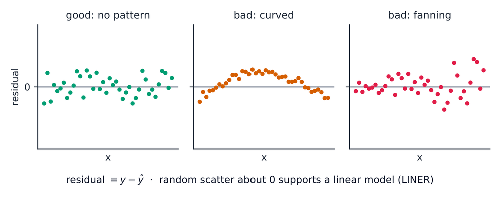
Syllabus
Enduring Understanding Learning Objective Essential Knowledge VAR-7
The $t$-distribution may be used to model variation.VAR-7.J
Identify the appropriate selection of a testing method for a slope of a regression model. [Skill 1.E]- VAR-7.J.1 The appropriate test for the slope of a regression model is a $t$-test for a slope.
VAR-7.K
Identify appropriate null and alternative hypotheses for a slope of a regression model. [Skill 1.F]- VAR-7.K.1 The null hypothesis for a $t$-test for a slope is: $H_0 : \beta = \beta_0$, where $\beta_0$ is the hypothesized value from the null hypothesis. The alternative hypothesis is $H_0 : \beta < \beta_0$ or $H_0 : \beta > \beta_0$, or $H_0 : \beta \neq \beta_0$.
VAR-7.L
Verify the conditions for the significance test for the slope of a regression model. [Skill 4.C]- VAR-7.L.1 In order to make statistical inferences when testing for the slope of a regression model, we must check the following:
- a. The true relationship between $x$ and $y$ is linear. Analysis of residuals may be used to verify linearity.
- b. The standard deviation for $y$, $\sigma_y$, does not vary with $x$. Analysis of residuals may be used to check for approximately equal standard deviations for all $x$.
- c. To check for independence:
- i. Data should be collected using a random sample or a randomized experiment.
- ii. When sampling without replacement, check that $n \le 10\% N$.
- d. For a particular value of $x$, the responses ($y$-values) are approximately normally distributed. Analysis of graphical representations of residuals may be used to check for normality.
- i. If the observed distribution is skewed, $n$ should be greater than 30.
- ii. If the sample size is less than 30, the distribution of the sample data should be free from strong skewness and outliers.
Source: College Board AP Course and Exam Description
The usual test asks whether there is any linear relationship:
$$H_0:\beta=0 \quad(\text{no linear relationship})\qquad H_a:\beta\neq 0 \ (\text{or } <,\,>).$$Check the LINER conditions. This is a $t$-test on the slope.Check residual plots before trusting a slope CI or test 9.5
Carrying Out a Test for a Slope
Syllabus
Enduring Understanding Learning Objective Essential Knowledge VAR-7
The $t$-distribution may be used to model variation.VAR-7.M
Calculate an appropriate test statistic for the slope of a regression model. [Skill 3.E]- VAR-7.M.1 The distribution of the slope of a regression model assuming all conditions are satisfied and the null hypothesis is true (null distribution) is a $t$-distribution.
- VAR-7.M.2 For simple linear regression when random sampling from a population for the response that can be modeled with a normal distribution for each value of the explanatory variable, the sampling distribution of $t = \dfrac{b - \beta}{SE_b}$ has a $t$-distribution with degrees of freedom equal to $n - 2$. When testing the slope in a simple linear regression model with one parameter, the slope, the test for the slope has $df = n - 1$.
DAT-3
Significance testing allows us to make decisions about hypotheses within a particular context.DAT-3.M
Interpret the $p$-value of a significance test for the slope of a regression model. [Skill 4.B]- DAT-3.M.1 An interpretation of the $p$-value of a significance test for the slope of a regression model should recognize that the $p$-value is computed by assuming that the null hypothesis is true, i.e., by assuming that the true population slope is equal to the particular value stated in the null hypothesis.
DAT-3.N
Justify a claim about the population based on the results of a significance test for the slope of a regression model. [Skill 4.E]- DAT-3.N.1 A formal decision explicitly compares the $p$-value to the significance $\alpha$. If the $p$-value $\le \alpha$, then reject the null hypothesis, $H_0 : \beta = \beta_0$. If the $p$-value $> \alpha$, then fail to reject the null hypothesis.
- DAT-3.N.2 The results of a significance test for the slope of a regression model can serve as the statistical reasoning to support the answer to a research question about that sample.
Source: College Board AP Course and Exam Description
The slope $t$ statistic:
$$t=\frac{b-0}{SE_b},\qquad df=n-2.$$Both $b$ and $SE_b$ come straight from the regression output. Find the $p$-value from the $t$-distribution, compare to $\alpha$, and conclude in context – evidence (or not) of a linear relationship between the two variables.Watch the tails. Regression output always prints the two-tailed $p$-value (for $H_a:\beta\neq 0$). If your $H_a$ is one-tailed, halve it – and first check the sample slope really points the way $H_a$ claims; if it points the other way, the one-tailed $p$-value is above $0.5$ and you cannot reject $H_0$.
Worked example. For the same output ($b=2.5$, $SE_b=0.8$, $n=20$), test $H_0:\beta=0$:
$$t=\frac{2.5-0}{0.8}=3.13,\qquad df=18,$$a small $p$-value ($<0.01$), so reject $H_0$ – convincing evidence of a linear relationship. This matches the interval, which excluded $0$.9.6
Selecting the Right Procedure
Syllabus
This topic is intended to focus on the skill of selecting an appropriate inference procedure now that students have a range of options. Students should be given opportunities to practice when and how to apply all learning objectives relating to inference.
Source: College Board AP Course and Exam Description
Across all of inference, identify: what is estimated or claimed (a proportion, a mean, a difference, a distribution of counts, or a slope), how many samples, and which design (independent or paired; sample or experiment). Then name the procedure, verify its conditions, carry it out, and communicate the conclusion with the statistic, the $p$-value or interval, and a plain-language answer in context. This selecting-and-communicating skill is what the investigative-task question rewards most.
9.6
Exam tips
- Inference for a slope tests whether the true slope is $0$ (no linear relationship).
- If a slope's confidence interval includes 0, you cannot conclude a real linear relationship – the variables may still be related in a curved way.
- Read the slope, standard error, t-statistic, and p-value straight from computer output – but the printed p-value is two-tailed, so halve it for a one-tailed $H_a$.
- Check the regression conditions (linearity, independence, roughly normal residuals, equal spread) via the residual plot.
- Interpret the interval and test in context, tied to the true slope.