Sampling Distributions

A statistic 统计量 (like a sample mean $\bar{x}$ or sample proportion $\hat{p}$) is computed from a sample and varies from sample to sample – this is sampling variability 抽样变异. A parameter 参数 ($\mu$ or $p$) is the fixed truth about the population. The sampling distribution 抽样分布 is the distribution of a statistic over all possible samples of a given size – it is the bridge from one sample to inference.

For large enough samples, many sampling distributions are approximately normal. That lets us describe a statistic by a center (its mean), a spread (its standard error 标准误), and a normal shape – and then compute how likely a given sample result is.

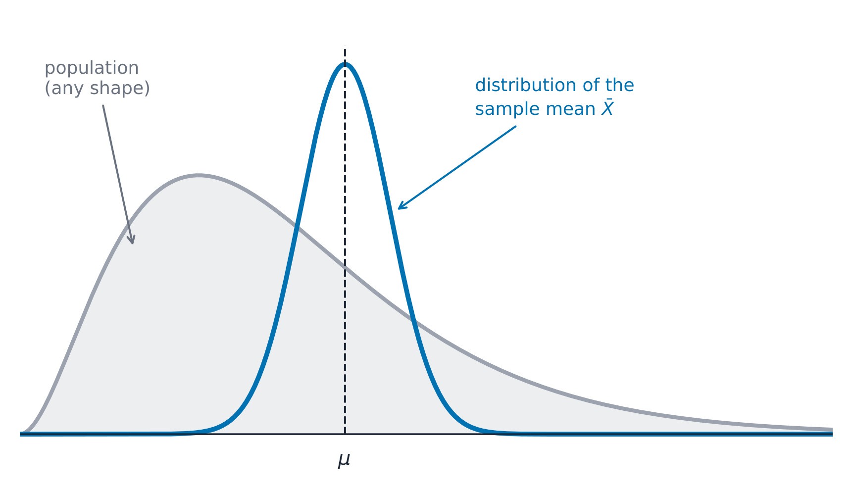
The Central Limit Theorem 中心极限定理 (CLT): for a sample mean, if the sample size $n$ is large enough (a common rule is $n\ge 30$), the sampling distribution of $\bar{x}$ is approximately normal, regardless of the population's shape. The larger $n$, the more normal and the tighter the distribution.

The sample mean is nearly normal whatever the shape of the population

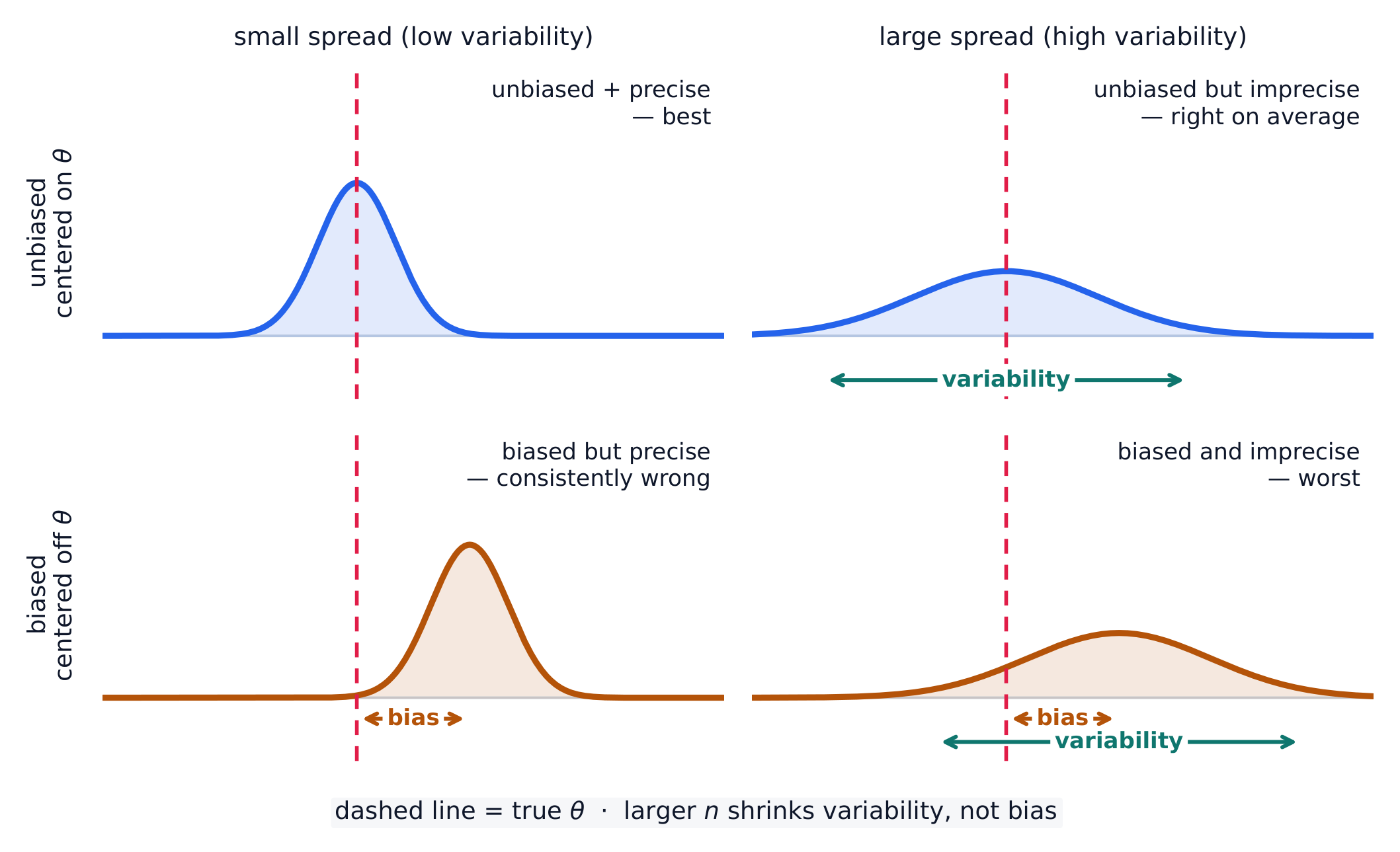
A statistic is unbiased 无偏 if the mean of its sampling distribution equals the parameter – it is correct on average. Bias is about the center being off; variability is about the spread. A good estimator is both unbiased (centered right) and low-variability (precise); larger samples reduce variability but do not fix bias from bad sampling.

For a sample proportion $\hat{p}$ from an SRS: the mean is $p$ (unbiased), and the standard deviation is

It is approximately normal when $np\ge 10$ and $n(1-p)\ge 10$ (the Large Counts condition), and the $10\%$ condition ($n\le 0.10N$) keeps the observations near-independent.

Worked example. Suppose $40\%$ of voters favor a measure ($p=0.4$) and you sample $n=100$. The standard error is $\sigma_{\hat p}=\sqrt{\dfrac{0.4(0.6)}{100}}=0.049$. The chance a sample gives $\hat{p}>0.5$ is $z=\dfrac{0.5-0.4}{0.049}=2.04$, so $P(\hat p>0.5)\approx0.02$ – a majority in the sample would be surprising.

For $\hat{p}_1-\hat{p}_2$ from two independent samples: the mean is $p_1-p_2$, and because the samples are independent the variances add:

It is approximately normal when the Large Counts condition holds in both samples.

For a sample mean $\bar{x}$ from an SRS: the mean is $\mu$ (unbiased), and the standard deviation is

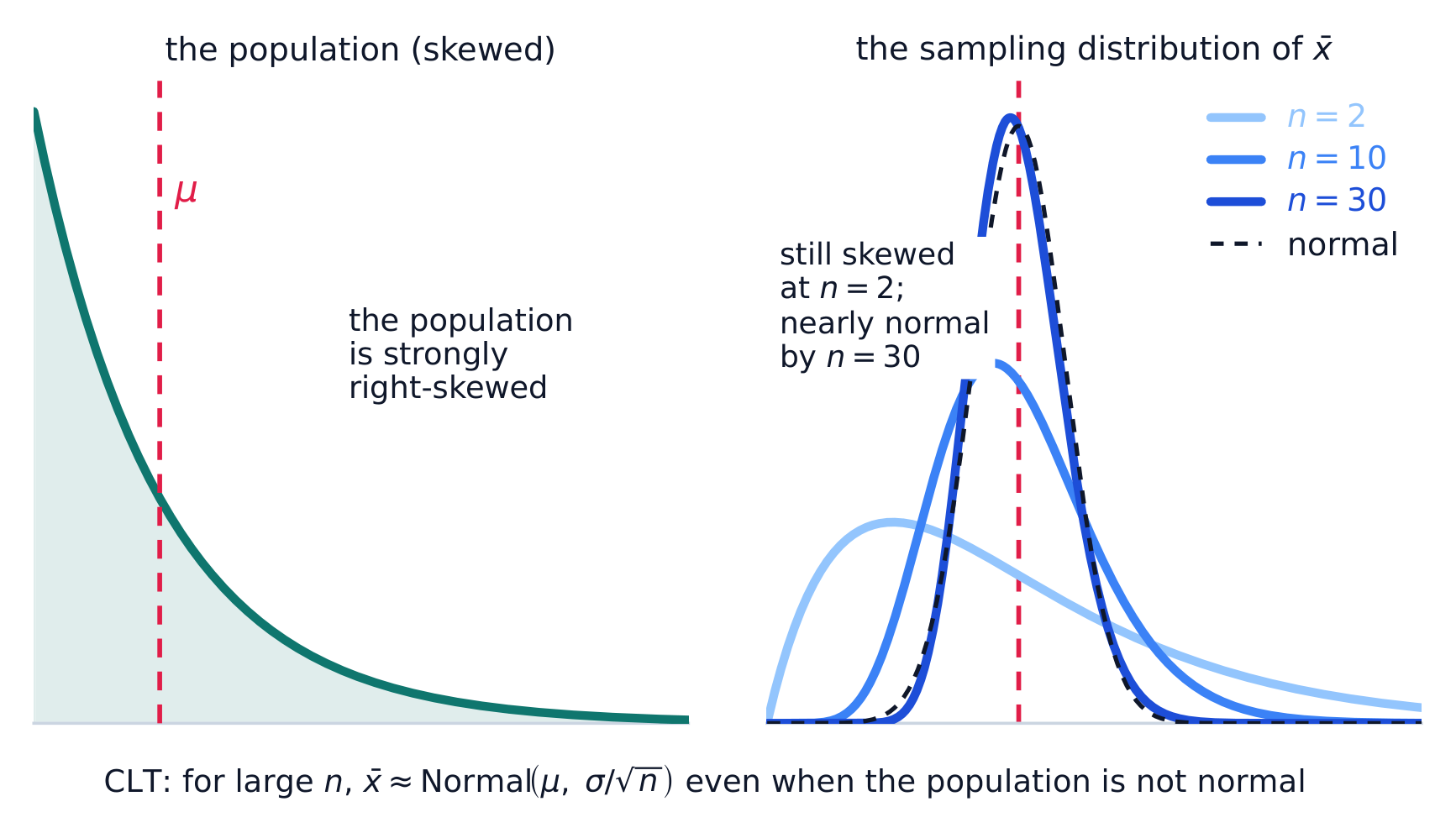
Its shape is normal if the population is normal, or approximately normal for large $n$ by the CLT. Note the spread shrinks like $\sqrt{n}$ – quadrupling the sample halves the standard error.

Worked example. A population has $\mu=70$ and $\sigma=12$. For samples of $n=36$, the sampling distribution of $\bar{x}$ is centered at $70$ with standard error $\dfrac{12}{\sqrt{36}}=2$. The chance a sample mean exceeds $73$ is $z=\dfrac{73-70}{2}=1.5$, so $P(\bar x>73)\approx0.067$.

All three sampling distributions are centered at $\mu$, but a larger $n$ makes the standard error $\sigma/\sqrt{n}$ smaller, so the distribution of $\bar{x}$ is taller and narrower.

For $\bar{x}_1-\bar{x}_2$ from two independent samples: the mean is $\mu_1-\mu_2$, and (independent, so variances add)

This is the foundation for two-sample inference in the next units.

• A sampling distribution is the distribution of a statistic over many samples, centered on the true parameter.
• The Central Limit Theorem: for a large enough sample the sample mean is approximately normal, even if the population is not.
• Larger samples give less variability (a smaller standard error).
• Check the conditions (random, independent/10%, large enough) before using a normal model.
• Keep straight what varies — the statistic — versus the fixed parameter.