Skip to content

Probability, Random Variables, and Probability Distributions

AP Statistics · Topic 4

Train
4.1

Random and Non-Random Patterns

Syllabus
Enduring UnderstandingLearning ObjectiveEssential Knowledge

VAR-1
Given that variation may be random or not, conclusions are uncertain.

VAR-1.F
Identify questions suggested by patterns in data. [Skill 1.A]

  • VAR-1.F.1 Patterns in data do not necessarily mean that variation is not random.

Source: College Board AP Course and Exam Description

Something is random 随机 if individual outcomes are uncertain but a regular pattern emerges over many repetitions. Short-run results look erratic; long-run relative frequencies settle down. This long-run stability is what makes probability useful.

Vocabulary Train
English Chinese Pinyin
random 随机 suí jī
4.2

Estimating Probabilities Using Simulation

Syllabus
Enduring UnderstandingLearning ObjectiveEssential Knowledge

UNC-2
Simulation allows us to anticipate patterns in data.

UNC-2.A
Estimate probabilities using simulation. [Skill 3.A]

  • UNC-2.A.1 A random process generates results that are determined by chance.
  • UNC-2.A.2 An outcome is the result of a trial of a random process.
  • UNC-2.A.3 An event is a collection of outcomes.
  • UNC-2.A.4 Simulation is a way to model random events, such that simulated outcomes closely match real-world outcomes. All possible outcomes are associated with a value to be determined by chance. Record the counts of simulated outcomes and the count total.
  • UNC-2.A.5 The relative frequency of an outcome or event in simulated or empirical data can be used to estimate the probability of that outcome or event.
  • UNC-2.A.6 The law of large numbers states that simulated (empirical) probabilities tend to get closer to the true probability as the number of trials increases.
    • Illustrative examples for UNC-2.A:
      • An outcome: Rolling a particular value on a six-sided number cube is one of six possible outcomes.
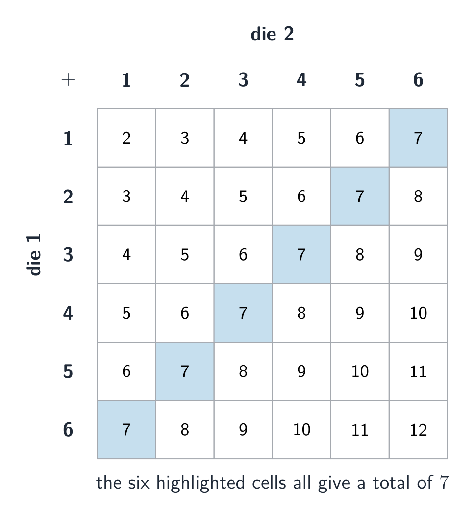
      • An event: When rolling two six-sided number cubes, an event would be a sum of seven. The corresponding collection of outcomes would be $(1, 6)$, $(2, 5)$, $(3, 4)$, $(4, 3)$, $(5, 2)$, and $(6, 1)$, where the ordered pairs indicate (face value on one cube, face value on the other cube).

Source: College Board AP Course and Exam Description

A simulation 模拟 imitates a chance process using random digits or technology. Steps: state the model, assign digits to outcomes, run many trials, and record the proportion of trials meeting the condition. The resulting proportion estimates the probability – more trials give a better estimate.

Vocabulary Train
English Chinese Pinyin
simulation 模拟 mó nǐ
4.3

Introduction to Probability

Syllabus
Enduring UnderstandingLearning ObjectiveEssential Knowledge

VAR-4
The likelihood of a random event can be quantified.

VAR-4.A
Calculate probabilities for events and their complements. [Skill 3.A]

  • VAR-4.A.1 The sample space of a random process is the set of all possible non-overlapping outcomes.
  • VAR-4.A.2 If all outcomes in the sample space are equally likely, then the probability an event E will occur is defined as the fraction: $\dfrac{\text{number of outcomes in event E}}{\text{total number of outcomes in sample space}}$
  • VAR-4.A.3 The probability of an event is a number between 0 and 1, inclusive.
  • VAR-4.A.4 The probability of the complement of an event E, $E'$ or $E^{C}$, (i.e., not E) is equal to $1 - P(E)$.

VAR-4.B
Interpret probabilities for events. [Skill 4.B]

  • VAR-4.B.1 Probabilities of events in repeatable situations can be interpreted as the relative frequency with which the event will occur in the long run.

Source: College Board AP Course and Exam Description

The probability 概率 of an event is a number from $0$ to $1$ giving its long-run relative frequency. The sample space 样本空间 is the set of all outcomes. For an event $A$, the complement rule: $P(A^c)=1-P(A)$. Probabilities of all outcomes sum to $1$.

Probability runs from 0 (impossible) to 1 (certain) Probability runs from 0 (impossible) to 1 (certain)

The four aces from a deck of playing cards A deck of cards is a classic source of probability: 52 equally likely outcomes make the chances easy to count

Explore

Explore probability with dice

Probability is the long-run fraction of times an outcome happens. Roll the dice many times and watch the experimental proportions settle toward the theoretical values.

Vocabulary Train
English Chinese Pinyin
probability 概率 gài lǜ
sample space 样本空间 yàng běn kōng jiān
complement
4.4

Mutually Exclusive Events

Syllabus
Enduring UnderstandingLearning ObjectiveEssential Knowledge

VAR-4
The likelihood of a random event can be quantified.

VAR-4.C
Explain why two events are (or are not) mutually exclusive. [Skill 4.B]

  • VAR-4.C.1 The probability that events $A$ and $B$ both will occur, sometimes called the joint probability, is the probability of the intersection of $A$ and $B$, denoted $P(A \cap B)$.
  • VAR-4.C.2 Two events are mutually exclusive or disjoint if they cannot occur at the same time. So $P(A \cap B) = 0$.

Source: College Board AP Course and Exam Description

Two events are mutually exclusive 互斥 (disjoint) if they cannot both happen. Then the addition rule simplifies:

$$P(A\text{ or }B)=P(A)+P(B)\quad(\text{if mutually exclusive}).$$
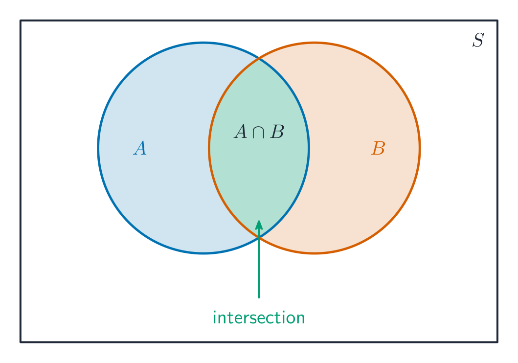
In general, $P(A\text{ or }B)=P(A)+P(B)-P(A\text{ and }B)$ – subtract the overlap so it is not counted twice.

A Venn diagram: the overlap is the intersection of two events A Venn diagram: the overlap is the intersection of two events

Vocabulary Train
English Chinese Pinyin
mutually exclusive 互斥 hù chì
4.5

Conditional Probability

Syllabus
Enduring UnderstandingLearning ObjectiveEssential Knowledge

VAR-4
The likelihood of a random event can be quantified.

VAR-4.D
Calculate conditional probabilities. [Skill 3.A]

  • VAR-4.D.1 The probability that event $A$ will occur given that event $B$ has occurred is called a conditional probability and denoted $P(A \mid B) = \dfrac{P(A \cap B)}{P(B)}$.
  • VAR-4.D.2 The multiplication rule states that the probability that events $A$ and $B$ both will occur is equal to the probability that event $A$ will occur multiplied by the probability that event $B$ will occur, given that $A$ has occurred. This is denoted $P(A \cap B) = P(A) \cdot P(B \mid A)$.

Source: College Board AP Course and Exam Description

Conditional probability

The conditional probability 条件概率 of $A$ given $B$ is

$$P(A\mid B)=\frac{P(A\text{ and }B)}{P(B)}.$$
It is the chance of $A$ once you know $B$ happened. Two-way tables make these easy: restrict to the row/column for $B$, then find $A$'s share.

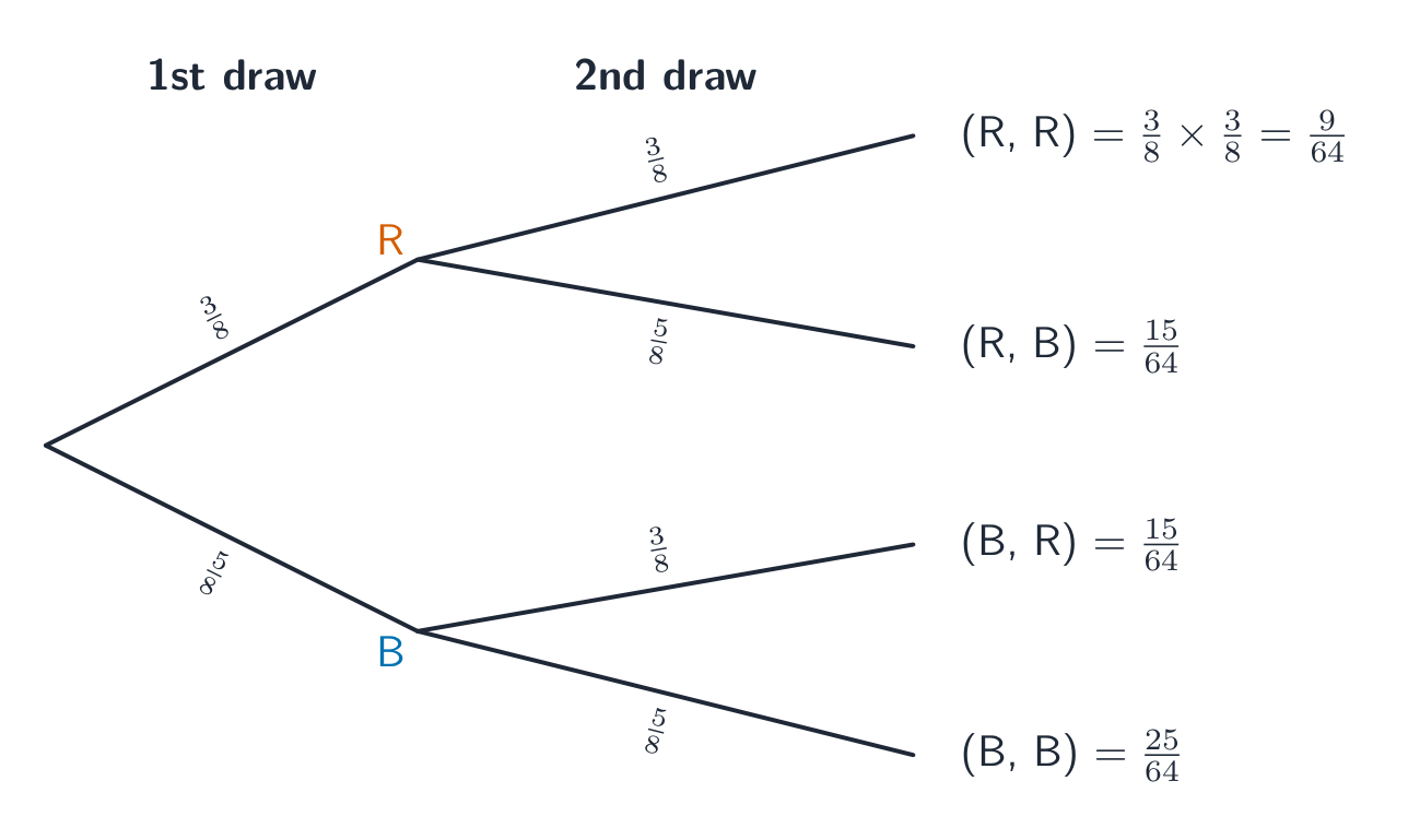
On a tree diagram, multiply the probabilities along the branches On a tree diagram, multiply the probabilities along the branches

Explore

Update a probability on new information

Conditional probability $P(B\mid A)$ is the chance of $B$ once you know $A$ happened. Change the branch probabilities and watch how conditioning reshapes the outcome.

Vocabulary Train
English Chinese Pinyin
conditional probability 条件概率 tiáo jiàn gài lǜ
4.6

Independent Events and Unions of Events
Syllabus
Enduring UnderstandingLearning ObjectiveEssential Knowledge

VAR-4
The likelihood of a random event can be quantified.

VAR-4.E
Calculate probabilities for independent events and for the union of two events. [Skill 3.A]

  • VAR-4.E.1 Events $A$ and $B$ are independent if, and only if, knowing whether event $A$ has occurred (or will occur) does not change the probability that event $B$ will occur.
  • VAR-4.E.2 If, and only if, events $A$ and $B$ are independent, then $P(A \mid B) = P(A)$, $P(B \mid A) = P(B)$, and $P(A \cap B) = P(A) \cdot P(B)$.
  • VAR-4.E.3 The probability that event $A$ or event $B$ (or both) will occur is the probability of the union of $A$ and $B$, denoted $P(A \cup B)$.
  • VAR-4.E.4 The addition rule states that the probability that event $A$ or event $B$ or both will occur is equal to the probability that event $A$ will occur plus the probability that event $B$ will occur minus the probability that both events $A$ and $B$ will occur. This is denoted $P(A \cup B) = P(A) + P(B) - P(A \cap B)$.

Source: College Board AP Course and Exam Description

Events are independent 独立 if knowing one does not change the other's probability: $P(A\mid B)=P(A)$. Then the multiplication rule simplifies:

$$P(A\text{ and }B)=P(A)\,P(B)\quad(\text{if independent}).$$
Independent is not the same as mutually exclusive – mutually exclusive events with nonzero probability are actually dependent (if one happens, the other cannot).

A sample space diagram lists every equally likely outcome A sample space diagram lists every equally likely outcome

Explore

Combine events with a Venn diagram

For a union $P(A\cup B)=P(A)+P(B)-P(A\cap B)$ — you subtract the overlap so it isn't counted twice. Switch the operation to see each region light up.

Vocabulary Train
English Chinese Pinyin
independent 独立 dú lì
4.7

Random Variables and Probability Distributions

Syllabus
Enduring UnderstandingLearning ObjectiveEssential Knowledge

VAR-5
Probability distributions may be used to model variation in populations.

VAR-5.A
Represent the probability distribution for a discrete random variable. [Skill 2.B]

  • VAR-5.A.1 The values of a random variable are the numerical outcomes of random behavior.
  • VAR-5.A.2 A discrete random variable is a variable that can only take a countable number of values. Each value has a probability associated with it. The sum of the probabilities over all of the possible values must be 1.
  • VAR-5.A.3 A probability distribution can be represented as a graph, table, or function showing the probabilities associated with values of a random variable.
  • VAR-5.A.4 A cumulative probability distribution can be represented as a table or function showing the probability of being less than or equal to each value of the random variable.
    • Illustrative examples for VAR-5.A: Outcomes of trials of a random process:
      • The sum of the outcomes for rolling two dice
      • The number of puppies in a randomly selected litter for a certain breed of dog

VAR-5.B
Interpret a probability distribution. [Skill 4.B]

  • VAR-5.B.1 An interpretation of a probability distribution provides information about the shape, center, and spread of a population and allows one to make conclusions about the population of interest.

Source: College Board AP Course and Exam Description

A random variable 随机变量 assigns a number to each outcome of a chance process. A probability distribution 概率分布 lists each possible value with its probability (they sum to $1$). A distribution can be discrete (a table of values) or continuous (an area-under-a-curve model like the normal).

Vocabulary Train
English Chinese Pinyin
random variable 随机变量 suí jī biàn liàng
probability distribution 概率分布 gài lǜ fēn bù
4.8

Mean and Standard Deviation of Random Variables

Syllabus
Enduring UnderstandingLearning ObjectiveEssential Knowledge

VAR-5
Probability distributions may be used to model variation in populations.

VAR-5.C
Calculate parameters for a discrete random variable. [Skill 3.B]

  • VAR-5.C.1 A numerical value measuring a characteristic of a population or the distribution of a random variable is known as a parameter, which is a single, fixed value.
  • VAR-5.C.2 The mean, or expected value, for a discrete random variable $X$ is $\mu_X = \sum x_i \cdot P(x_i)$.
  • VAR-5.C.3 The standard deviation for a discrete random variable $X$ is $\sigma_X = \sqrt{\sum (x_i - \mu_x)^2 \cdot P(x_i)}$.

VAR-5.D
Interpret parameters for a discrete random variable. [Skill 4.B]

  • VAR-5.D.1 Parameters for a discrete random variable should be interpreted using appropriate units and within the context of a specific population.

Source: College Board AP Course and Exam Description

The mean (expected value) 期望值 of a discrete random variable is the probability-weighted average:

$$\mu_X=E(X)=\sum x_i\,P(x_i).$$
The standard deviation $\sigma_X=\sqrt{\sum (x_i-\mu_X)^2\,P(x_i)}$ measures typical spread from the mean. The expected value is the long-run average outcome, not a value you expect on any single trial.

Worked example. A game pays $\$5$ with probability $0.2$ and costs you $\$1$ (a $-1$ outcome) with probability $0.8$. The expected value is

$$E(X)=5(0.2)+(-1)(0.8)=1-0.8=\$0.20,$$
so over many plays you gain about $20$ cents per play on average, even though no single play gives exactly that.

Vocabulary Train
English Chinese Pinyin
mean (expected value) 期望值 qī wàng zhí
4.9

Combining Random Variables

Syllabus
Enduring UnderstandingLearning ObjectiveEssential Knowledge

VAR-5
Probability distributions may be used to model variation in populations.

VAR-5.E
Calculate parameters for linear combinations of random variables. [Skill 3.B]

  • VAR-5.E.1 For random variables $X$ and $Y$ and real numbers $a$ and $b$, the mean of $aX + bY$ is $a\mu_x + b\mu_y$.
  • VAR-5.E.2 Two random variables are independent if knowing information about one of them does not change the probability distribution of the other.
  • VAR-5.E.3 For independent random variables $X$ and $Y$ and real numbers $a$ and $b$, the mean of $aX + bY$ is $a\mu_x + b\mu_y$, and the variance of $aX + bY$ is $a^2\sigma^2_x + b^2\sigma^2_y$.

VAR-5.F
Describe the effects of linear transformations of parameters of random variables. [Skill 3.C]

  • VAR-5.F.1 For $Y = a + bX$, the probability distribution of the transformed random variable, $Y$, has the same shape as the probability distribution for $X$, so long as $a > 0$ and $b > 0$. The mean of $Y$ is $\mu_y = a + b\mu_x$. The standard deviation of $Y$ is $\sigma_y = |b|\sigma_x$.

Source: College Board AP Course and Exam Description

When you add or subtract random variables, means add: $\mu_{X\pm Y}=\mu_X\pm\mu_Y$. If $X$ and $Y$ are independent, variances add (even when subtracting):

$$\sigma^2_{X\pm Y}=\sigma^2_X+\sigma^2_Y.$$
Take the square root for the standard deviation. Also, scaling: $\mu_{aX+b}=a\mu_X+b$ and $\sigma_{aX+b}=|a|\sigma_X$.

4.10

Introduction to the Binomial Distribution
Syllabus
Enduring UnderstandingLearning ObjectiveEssential Knowledge

UNC-3
Probabilistic reasoning allows us to anticipate patterns in data.

UNC-3.A
Estimate probabilities of binomial random variables using data from a simulation. [Skill 3.A]

  • UNC-3.A.1 A probability distribution can be constructed using the rules of probability or estimated with a simulation using random number generators.
  • UNC-3.A.2 A binomial random variable, $X$, counts the number of successes in $n$ repeated independent trials, each trial having two possible outcomes (success or failure), with the probability of success $p$ and the probability of failure $1 - p$.

UNC-3.B
Calculate probabilities for a binomial distribution. [Skill 3.A]

  • UNC-3.B.1 The probability that a binomial random variable, $X$, has exactly $x$ successes for $n$ independent trials, when the probability of success is $p$, is calculated as $P(X = x) = \binom{n}{x} p^x (1 - p)^{n-x}, x = 0, 1, 2, \ldots, n$. This is the binomial probability function.

Source: College Board AP Course and Exam Description

The binomial distribution

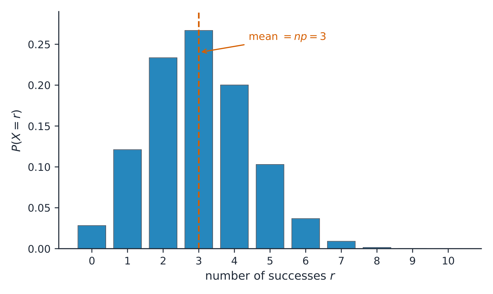
A binomial 二项 setting (BINS): a fixed number $n$ of Independent trials, each with two outcomes (success/failure) and the same success probability $p$. The random variable $X=$ number of successes. Its probability:

$$P(X=k)=\binom{n}{k}p^k(1-p)^{n-k}.$$

The binomial distribution, with mean n times p The binomial distribution, with mean n times p

Explore

Shape a binomial distribution

A binomial distribution counts successes in $n$ independent trials each with probability $p$. Change $n$ and $p$ and watch the bars shift and spread.

Vocabulary Train
English Chinese Pinyin
binomial 二项 èr xiàng
Exercise sheet
4.11

Parameters for a Binomial Distribution

Syllabus
Enduring UnderstandingLearning ObjectiveEssential Knowledge

UNC-3
Probabilistic reasoning allows us to anticipate patterns in data.

UNC-3.C
Calculate parameters for a binomial distribution. [Skill 3.B]

  • UNC-3.C.1 If a random variable is binomial, its mean, $\mu_x$, is $np$ and its standard deviation, $\sigma_x$, is $\sqrt{np(1 - p)}$.

UNC-3.D
Interpret probabilities and parameters for a binomial distribution. [Skill 4.B]

  • UNC-3.D.1 Probabilities and parameters for a binomial distribution should be interpreted using appropriate units and within the context of a specific population or situation.

Source: College Board AP Course and Exam Description

For a binomial $X$ with $n$ trials and success probability $p$:

$$\mu_X=np,\qquad \sigma_X=\sqrt{np(1-p)}.$$
Use these for "how many successes do we expect, and how much do they vary" questions.

Worked example. A player makes $70\%$ of free throws. In $n=10$ shots, the probability of exactly $8$ makes is

$$P(X=8)=\binom{10}{8}(0.7)^8(0.3)^2=45\times0.0576\times0.09\approx0.23,$$
and the expected number of makes is $\mu=np=10(0.7)=7$, with $\sigma=\sqrt{10(0.7)(0.3)}\approx1.45$.

4.12

The Geometric Distribution

Syllabus
Enduring UnderstandingLearning ObjectiveEssential Knowledge

UNC-3
Probabilistic reasoning allows us to anticipate patterns in data.

UNC-3.E
Calculate probabilities for geometric random variables. [Skill 3.A]

  • UNC-3.E.1 For a sequence of independent trials, a geometric random variable, $X$, gives the number of the trial on which the first success occurs. Each trial has two possible outcomes (success or failure) with the probability of success $p$ and the probability of failure $1 - p$.
  • UNC-3.E.2 The probability that the first success for repeated independent trials with probability of success $p$ occurs on trial $x$ is calculated as $P(X = x) = (1 - p)^{x-1} p, x = 1, 2, 3, \ldots$. This is the geometric probability function.

UNC-3.F
Calculate parameters of a geometric distribution. [Skill 3.B]

  • UNC-3.F.1 If a random variable is geometric, its mean, $\mu_x$, is $\dfrac{1}{p}$ and its standard deviation, $\sigma_x$, is $\dfrac{\sqrt{(1 - p)}}{p}$.

UNC-3.G
Interpret probabilities and parameters for a geometric distribution. [Skill 4.B]

  • UNC-3.G.1 Probabilities and parameters for a geometric distribution should be interpreted using appropriate units and within the context of a specific population or situation.

Source: College Board AP Course and Exam Description

A geometric 几何 setting is the same as binomial but with no fixed $n$: you keep trying until the first success. The random variable $Y=$ the trial of the first success:

$$P(Y=k)=(1-p)^{k-1}\,p,\qquad \mu_Y=\frac{1}{p}.$$
So the expected number of trials until the first success is $1/p$.

Vocabulary Train
English Chinese Pinyin
geometric 几何 jǐ hé
4.12

Exam tips

  • A probability lies in $[0,1]$; use the complement ($1-P$) and add mutually exclusive events.
  • For independent events multiply; for "and/or" use the general addition and conditional rules.
  • Expected value = $\sum(\text{value}\times\text{probability})$.
  • Recognise binomial (fixed $n$, two outcomes, constant $p$) and geometric settings.
  • Draw a tree or table for multi-stage problems and multiply along branches.

Log in or create account

IGCSE & A-Level