Skip to content · ⁨ข้ามไปยังเนื้อหา⁩

Exploring Two-Variable Data · ⁨การสำรวจข้อมูลสองตัวแปร⁩

AP Statistics · Topic 2 · ⁨หัวข้อ 2⁩

Video lesson for this topic · ⁨บทเรียนวิดีโอสำหรับหัวข้อนี้⁩ Open the video page · ⁨เปิดหน้าวิดีโอ⁩
7:49

การสำรวจข้อมูลสองตัวแปร

เด็กสามสิบคนจากโรงเรียนประถมแห่งหนึ่ง สำหรับแต่ละคน มีสองตัวเลข: ขนาดรองเท้า และคะแนนการอ่าน ทดลองวางจุดหนึ่งต่อหนึ่งเด็ก รูปแบบนี้ยากที่จะ...

English narration · English + 中文 subtitles burned in · ⁨การบรรยายภาษาอังกฤษ · คำบรรยายภาษาอังกฤษ + 中文 ลอยตัวบนภาพ⁩

2.1

Are Two Variables Related? · ⁨ตัวแปรสองตัวมีความสัมพันธ์กันหรือไม่?⁩

Syllabus · ⁨หลักสูตร⁩
English
Enduring UnderstandingLearning ObjectiveEssential Knowledge

VAR-1
Given that variation may be random or not, conclusions are uncertain.

VAR-1.D
Identify questions to be answered about possible relationships in data. [Skill 1.A]

  • VAR-1.D.1 Apparent patterns and associations in data may be random or not.
ไทย

ความเข้าใจที่ยั่งยืน (VAR-1): เนื่องจากความแปรปรวนอาจเป็นแบบสุ่มหรือไม่ ดังนั้นข้อสรุปจึงมีความไม่แน่นอน

Learning ObjectiveEssential Knowledge

VAR-1.D
ระบุคำถามที่จะตอบเกี่ยวกับความสัมพันธ์ที่เป็นไปได้ในข้อมูล [Skill 1.A]

  • VAR-1.D.1 ลวดลายและความสัมพันธ์ที่ปรากฏในข้อมูลอาจเป็นแบบสุ่มหรือไม่ก็ตาม

Source: College Board AP Course and Exam Description · ⁨แหล่งที่มา: คำอธิบายหลักสูตรและข้อสอบ College Board AP⁩

English

Two-variable data let us ask whether two characteristics are associated 关联 – whether knowing one tells you something about the other. An explanatory variable 解释变量 (the "input") may help predict a response variable 响应变量 (the "output"). Association is not the same as causation.

ไทย

ข้อมูลสองตัวแปรช่วยให้เราถามได้ว่าลักษณะสองอย่าง มีความสัมพันธ์ หรือไม่ – ว่าการรู้สิ่งหนึ่งบอกอะไรเกี่ยวกับอีกสิ่งหนึ่งได้หรือไม่. ตัวแปรอธิบาย (“อินพุต”) อาจช่วยทำนาย ตัวแปรตอบสนอง (“เอาต์พุต”). ความสัมพันธ์ไม่เท่ากับสาเหตุ.

2.2

Two Categorical Variables · ⁨ตัวแปรเชิงหมวดหมู่สองชนิด⁩

Syllabus · ⁨หลักสูตร⁩
English
Enduring UnderstandingLearning ObjectiveEssential Knowledge

UNC-1
Graphical representations and statistics allow us to identify and represent key features of data.

UNC-1.P
Compare numerical and graphical representations for two categorical variables. [Skill 2.D]

  • UNC-1.P.1 Side-by-side bar graphs, segmented bar graphs, and mosaic plots are examples of bar graphs for one categorical variable, broken down by categories of another categorical variable.
  • UNC-1.P.2 Graphical representations of two categorical variables can be used to compare distributions and/or determine if variables are associated.
  • UNC-1.P.3 A two-way table, also called a contingency table, is used to summarize two categorical variables. The entries in the cells can be frequency counts or relative frequencies.
  • UNC-1.P.4 A joint relative frequency is a cell frequency divided by the total for the entire table.
ไทย

ความเข้าใจที่ยั่งยืน (UNC-1): กราฟและสถิติช่วยให้เราระบุและแสดงคุณลักษณะสำคัญของข้อมูลได้

Learning ObjectiveEssential Knowledge

UNC-1.P
เปรียบเทียบการแสดงแบบตัวเลขและกราฟิกสำหรับตัวแปรเชิงหมวดหมู่สองตัว [Skill 2.D]

  • UNC-1.P.1 Side-by-side bar graphs, segmented bar graphs, และ mosaic plots เป็นตัวอย่างของ bar graphs สำหรับตัวแปรเชิงหมวดหมู่หนึ่งตัว ที่แยกย่อยตาม categories ของอีกตัวแปรเชิงหมวดหมู่หนึ่ง
  • UNC-1.P.2 การแสดงแบบกราฟิกของตัวแปรเชิงหมวดหมู่สองตัวสามารถใช้เพื่อเปรียบเทียบการกระจายและ/หรือตรวจสอบว่าตัวแปรสัมพันธ์กันหรือไม่
  • UNC-1.P.3 ตารางสองทาง หรือที่เรียกว่าตารางความถ่วง (contingency table) ใช้สำหรับสรุปตัวแปรเชิงหมวดหมู่สองตัว ค่าในเซลล์สามารถเป็นจำนวนความถี่หรือความถี่สัมพัทธ์ได้
  • UNC-1.P.4 ความถี่สัมพัทธ์ร่วม (joint relative frequency) คือความถี่ของเซลล์หารด้วยผลรวมทั้งหมดของตารางทั้งตาราง

Source: College Board AP Course and Exam Description · ⁨แหล่งที่มา: คำอธิบายหลักสูตรและข้อสอบ College Board AP⁩

English

A two-way table 双向表 (contingency table) counts individuals by two categorical variables at once. A marginal distribution 边缘分布 is a row or column total written as a fraction of the grand total (the totals themselves are just counts). Comparing the inside cells shows whether the variables are related.

ไทย

ตารางสองมิติ (ตารางความถ่วง) นับจำนวนบุคคลตามตัวแปรเชิงหมวดหมู่สองชนิดพร้อมกัน. การแจกแจงขอบ คือผลรวมแถวหรือคอลัมน์ที่เขียนเป็นเศษส่วนของผลรวมทั้งหมด (ผลรวมเองเป็นเพียงจำนวนนับ). การเปรียบเทียบเซลล์ด้านในแสดงว่าตัวแปรทั้งสองมีความสัมพันธ์กันหรือไม่.

2.3

Comparing Groups with Conditional Distributions · ⁨เปรียบเทียบกลุ่มด้วยการแจกแจงแบบเงื่อนไข⁩

Syllabus · ⁨หลักสูตร⁩
English

Enduring Understanding (UNC-1): Graphical representations and statistics allow us to identify and represent key features of data.

Learning Objective UNC-1.Q: Calculate statistics for two categorical variables. [Skill 2.C]

  • UNC-1.Q.1 The marginal relative frequencies are the row and column totals in a two-way table divided by the total for the entire table.
  • UNC-1.Q.2 A conditional relative frequency is a relative frequency for a specific part of the contingency table (e.g., cell frequencies in a row divided by the total for that row).

Learning Objective UNC-1.R: Compare statistics for two categorical variables. [Skill 2.D]

  • UNC-1.R.1 Summary statistics for two categorical variables can be used to compare distributions and/or determine if variables are associated.
ไทย

ความเข้าใจที่ยั่งยืน (UNC-1): กราฟและสถิติช่วยให้เราระบุและแสดงคุณลักษณะสำคัญของข้อมูลได้

วัตถุประสงค์การเรียนรู้ UNC-1.Q: คำนวณสถิติสำหรับตัวแปรเชิงหมวดหมู่สองตัว [ทักษะ 2.C]

  • UNC-1.Q.1 ความถี่สัมพัทธ์ขอบ (marginal relative frequencies) คือผลรวมตามแถวและคอลัมน์ในตารางสองทางหารด้วยผลรวมทั้งหมดของตารางทั้งตาราง
  • UNC-1.Q.2 ความถี่สัมพัทธ์เงื่อนไข (conditional relative frequency) คือความถี่สัมพัทธ์สำหรับส่วนเฉพาะหนึ่งของตารางความถ่วง (เช่น ความถี่ของเซลล์ในแถวหารด้วยผลรวมของแถวนั้น)

วัตถุประสงค์การเรียนรู้ UNC-1.R: เปรียบเทียบสถิติสำหรับตัวแปรเชิงหมวดหมู่สองตัว [ทักษะ 2.D]

  • UNC-1.R.1 สถิติสรุปสำหรับตัวแปรเชิงหมวดหมู่สองตัวสามารถใช้เพื่อเปรียบเทียบการแจกแจงและ/หรือตรวจสอบว่าตัวแปรมีความสัมพันธ์กันหรือไม่

Source: College Board AP Course and Exam Description · ⁨แหล่งที่มา: คำอธิบายหลักสูตรและข้อสอบ College Board AP⁩

English

A conditional distribution 条件分布 is the distribution of one variable within a fixed category of the other (found by dividing each cell by its row or column total). If the conditional distributions differ across groups, the two variables are associated; if they are the same, there is no association. Segmented bar charts 分段条形图 or mosaic plots display them.

ไทย

การแจกแจงแบบเงื่อนไข คือการแจกแจงของตัวแปรหนึ่ง ภายใน หมวดหมู่คงที่ของอีกตัวแปรหนึ่ง (หาได้โดยการหารแต่ละเซลล์ด้วยผลรวมแถวหรือคอลัมน์). หากการแจกแจงแบบเงื่อนไขแตกต่างกันข้ามกลุ่ม ตัวแปรทั้งสองจะ มีความสัมพันธ์; หากเหมือนกัน ไม่มีความสัมพันธ์. แผนภาพแท่งแบ่งส่วน หรือแผนภาพโมเสกแสดงการแจกแจงเหล่านี้.
2.4

Scatterplots for Two Quantitative Variables · ⁨แผนภาพกระจายสำหรับตัวแปรเชิงปริมาณสองชนิด⁩

Syllabus · ⁨หลักสูตร⁩
English

Enduring Understanding (UNC-1): Graphical representations and statistics allow us to identify and represent key features of data.

Learning Objective UNC-1.S: Represent bivariate quantitative data using scatterplots. [Skill 2.B]

  • UNC-1.S.1 A bivariate quantitative data set consists of observations of two different quantitative variables made on individuals in a sample or population.
  • UNC-1.S.2 A scatterplot shows two numeric values for each observation, one corresponding to the value on the $x$-axis and one corresponding to the value on the $y$-axis.
  • UNC-1.S.3 An explanatory variable is a variable whose values are used to explain or predict corresponding values for the response variable.

Enduring Understanding (DAT-1): Regression models may allow us to predict responses to changes in an explanatory variable.

Learning Objective DAT-1.A: Describe the characteristics of a scatter plot. [Skill 2.A]

  • DAT-1.A.1 A description of a scatter plot includes form, direction, strength, and unusual features.
  • DAT-1.A.2 The direction of the association shown in a scatterplot, if any, can be described as positive or negative.
  • DAT-1.A.3 A positive association means that as values of one variable increase, the values of the other variable tend to increase. A negative association means that as values of one variable increase, values of the other variable tend to decrease.
  • DAT-1.A.4 The form of the association shown in a scatterplot, if any, can be described as linear or non-linear to varying degrees.
  • DAT-1.A.5 The strength of the association is how closely the individual points follow a specific pattern, e.g., linear, and can be shown in a scatterplot. Strength can be described as strong, moderate, or weak.
  • DAT-1.A.6 Unusual features of a scatter plot include clusters of points or points with relatively large discrepancies between the value of the response variable and a predicted value for the response variable.
ไทย

ความเข้าใจที่ยั่งยืน (UNC-1): กราฟและสถิติช่วยให้เราระบุและแสดงคุณลักษณะสำคัญของข้อมูลได้

วัตถุประสงค์การเรียนรู้ UNC-1.S: แสดงข้อมูลเชิงปริมาณคู่โดยใช้กราฟกระจาย [ทักษะ 2.B]

  • UNC-1.S.1 ชุดข้อมูลเชิงปริมาณคู่ประกอบด้วยข้อสังเกตของตัวแปรเชิงปริมาณสองตัวที่แตกต่างกันซึ่งวัดจากบุคคลในตัวอย่างหรือประชากร
  • UNC-1.S.2 กราฟกระจายแสดงค่าตัวเลขสองค่าสำหรับแต่ละข้อสังเกต โดยค่าหนึ่งสอดคล้องกับค่าบน $x$-แกน และอีกค่าหนึ่งสอดคล้องกับค่าบน $y$-แกน
  • UNC-1.S.3 ตัวแปรอธิบายคือตัวแปรwhose values被用来解释或预测响应变量。

ความเข้าใจที่ยั่งยืน (DAT-1): แบบจำลองการถดถอยอาจช่วยให้เราทำนายผลลัพธ์จากการเปลี่ยนแปลงในตัวแปรอธิบายได้

วัตถุประสงค์การเรียนรู้ DAT-1.A: อธิบายลักษณะของกราฟกระจาย [ทักษะ 2.A]

  • DAT-1.A.1 การอธิบายกราฟกระจายประกอบด้วยรูปแบบ ทิศทาง ความเข้ม และลักษณะผิดปกติ
  • DAT-1.A.2 ทิศทางของความสัมพันธ์ที่ปรากฏในกราฟกระจาย หากมี สามารถอธิบายได้ว่าเป็นบวกหรือลบ
  • DAT-1.A.3 ความสัมพันธ์เชิงบวกหมายความว่าเมื่อค่าของตัวแปรหนึ่งเพิ่มขึ้น ค่าของอีกตัวแปรหนึ่งก็มีแนวโน้มที่จะเพิ่มขึ้น ความสัมพันธ์เชิงลบหมายความว่าเมื่อค่าของตัวแปรหนึ่งเพิ่มขึ้น ค่าของอีกตัวแปรหนึ่งมีแนวโน้มที่จะลดลง
  • DAT-1.A.4 รูปแบบของความสัมพันธ์ที่ปรากฏในกราฟกระจาย หากมี สามารถอธิบายได้ว่ามีความเป็นเส้นตรงหรือไม่เป็นเส้นตรงในระดับต่างๆ
  • DAT-1.A.5 ความเข้มของความสัมพันธ์คือระดับที่จุดแต่ละจุดปฏิบัติตามรูปแบบเฉพาะ เช่น เส้นตรง ในกราฟกระจาย ความเข้มสามารถอธิบายได้ว่าแข็งแกร่ง ปานกลาง หรืออ่อน
  • DAT-1.A.6 ลักษณะผิดปกติของกราฟกระจายรวมถึงกลุ่มของจุดหรือจุดที่มีข้อแตกต่างอย่างมีนัยสำคัญระหว่างค่าของตัวแปรตอบสนองกับค่าที่คาดหมายสำหรับตัวแปรตอบสนอง

Source: College Board AP Course and Exam Description · ⁨แหล่งที่มา: คำอธิบายหลักสูตรและข้อสอบ College Board AP⁩

English

A scatterplot 散点图 plots each individual as a point, explanatory variable on the $x$-axis and response on the $y$-axis. Describe it with DUFS: Direction (positive/negative), Unusual features (outliers, clusters), Form (linear or curved), and Strength (how tightly the points follow the pattern) – always in context.

ไทย

กราฟกระจาย (scatterplot) แสดงแต่ละบุคคลเป็นจุด โดยตัวแปรอธิบายวางบน $x$ และตัวแปรตอบรับวางบน $y$ อธิบายด้วย DUFS: ทิศทาง (บวก/ลบ), ลักษณะผิดปกติ (ค่าสุดขั้ว, กลุ่ม), รูปแบบ (เชิงเส้นหรือโค้ง), และ ความเข้ม (ความแน่นที่จุดตามรูปแบบ) – ต้องอธิบายในบริบทเสมอ

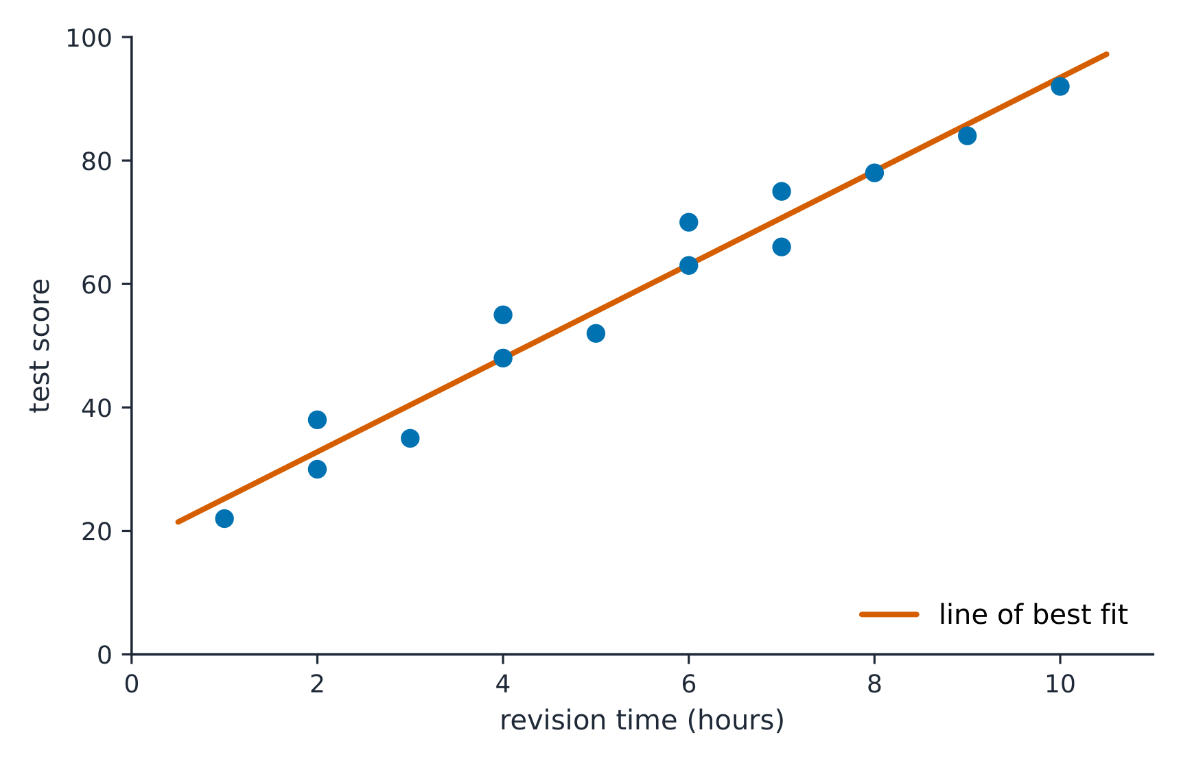
เส้นประมาณการที่ดีที่สุดวิ่งผ่านกลางกลุ่มจุดกระจาย
Vocabulary · ⁨คำศัพท์⁩ Train · ⁨ฝึกฝน⁩
English ไทย
associated/əˈsəʊsɪeɪtɪd/ มีความสัมพันธ์กัน
explanatory variable/ekˈsplænətəri ˈveərɪəbl/ explanatory variable
response variable/rɪˈspɒns ˈveərɪəbl/ response variable
two-way table/tuː weɪ ˈteɪbl/ ตารางสองมิติ
marginal distributions/ˈmɑːdʒɪnl ˌdɪstrɪˈbjuːʃnz/ การแจกแจงส่วนขอบ
conditional distribution/kənˈdɪʃənl ˌdɪstrɪˈbjuːʃn/ การแจกแจงแบบมีเงื่อนไข
Segmented bar charts/seɡˈmentɪd bɑː tʃɑːts/ แผนภูมิแท่งแบบแบ่งส่วน
scatterplot/ˈskætəplɒt/ แผนภูมิกระจาย (scatterplot)
2.5

Correlation · ⁨ความสัมพันธ์⁩

Syllabus · ⁨หลักสูตร⁩
English

Enduring Understanding (DAT-1): Regression models may allow us to predict responses to changes in an explanatory variable.

Learning Objective DAT-1.B: Determine the correlation for a linear relationship. [Skill 2.C]

  • DAT-1.B.1 The correlation, $r$, gives the direction and quantifies the strength of the linear association between two quantitative variables.
  • DAT-1.B.2 The correlation coefficient can be calculated by: $r = \dfrac{1}{n-1} \sum \left( \dfrac{x_i - \bar{x}}{s_x} \right) \left( \dfrac{y_i - \bar{y}}{s_y} \right)$. However, the most common way to determine $r$ is by using technology.
  • DAT-1.B.3 A correlation coefficient close to 1 or $-1$ does not necessarily mean that a linear model is appropriate.

Learning Objective DAT-1.C: Interpret the correlation for a linear relationship. [Skill 4.B]

  • DAT-1.C.1 The correlation, $r$, is unit-free, and always between $-1$ and 1, inclusive. A value of $r = 0$ indicates that there is no linear association. A value of $r = 1$ or $r = -1$ indicates that there is a perfect linear association.
  • DAT-1.C.2 A perceived or real relationship between two variables does not mean that changes in one variable cause changes in the other. That is, correlation does not necessarily imply causation.
ไทย

ความเข้าใจที่ยั่งยืน (DAT-1): แบบจำลองการถดถอยอาจช่วยให้เราทำนายผลลัพธ์จากการเปลี่ยนแปลงในตัวแปรอธิบายได้

วัตถุประสงค์การเรียนรู้ DAT-1.B: หาค่าสหประสิทธิผลสำหรับความสัมพันธ์เชิงเส้น [ทักษะ 2.C]

  • DAT-1.B.1 สหประสิทธิผล, $r$, บอกลักษณะทิศทางและวัดระดับความเข้มของความสัมพันธ์เชิงเส้นระหว่างตัวแปรเชิงปริมาณสองตัว
  • DAT-1.B.2 ค่าสัมประสิทธิ์สหสัมพันธ์สามารถคำนวณได้ด้วยสูตร: $r = \dfrac{1}{n-1} \sum \left( \dfrac{x_i - \bar{x}}{s_x} \right) \left( \dfrac{y_i - \bar{y}}{s_y} \right)$ อย่างไรก็ตาม วิธีที่พบบ่อยที่สุดในการหาค่า $r$ คือการใช้เทคโนโลยี
  • DAT-1.B.3 ค่าสัมประสิทธิ์สหประสิทธิผลที่ใกล้กับ 1 หรือ $-1$ ไม่จำเป็นต้องหมายความว่าแบบจำลองเชิงเส้นเหมาะสม

วัตถุประสงค์การเรียนรู้ DAT-1.C: ตีความค่าสหประสิทธิผลสำหรับความสัมพันธ์เชิงเส้น [ทักษะ 4.B]

  • DAT-1.C.1 สหประสิทธิผล, $r$, เป็นปริมาณไม่มีหน่วย และอยู่ระหว่าง $-1$ ถึง 1 เสมอ ค่าของ $r = 0$ แสดงว่าไม่มีความสัมพันธ์เชิงเส้น ค่าของ $r = 1$ หรือ $r = -1$ แสดงว่ามีความสัมพันธ์เชิงเส้นสมบูรณ์
  • DAT-1.C.2 ความสัมพันธ์ที่รับรู้หรือมีความจริงระหว่างตัวแปรสองตัว并不意味着改变一个变量会导致另一个变量的变化。即,相关性并不必然意味着因果关系。

Source: College Board AP Course and Exam Description · ⁨แหล่งที่มา: คำอธิบายหลักสูตรและข้อสอบ College Board AP⁩

English
What r actually measures

The correlation coefficient 相关系数 $r$ measures the strength and direction of a linear relationship. It runs from $-1$ to $1$: near $\pm 1$ is strong linear, near $0$ is weak linear. $r$ has no units and does not change if you swap the variables. Warnings: $r$ only measures linear strength, it is not resistant to outliers, and a strong $r$ does not prove causation.

ไทย
r วัดอะไรจริงๆ

สัมประสิทธิ์สหสัมพันธ์ (correlation coefficient) $r$ วัด ความเข้มแข็งและทิศทางของความสัมพันธ์แบบเส้นตรง.它有值从 $-1$ ถึง $1$: Near $\pm 1$ means strong linear relationship, near $0$ means weak linear relationship. $r$ ไม่มีหน่วยและไม่เปลี่ยนเมื่อสลับตัวแปร ข้อควรระวัง: $r$ วัด ความเข้มแข็งแบบเส้นตรง เท่านั้น, ไม่ทนทานต่อค่าผิดปกติ, และค่า $r$ ที่สูง ไม่ได้ บ่งชี้ถึงความสัมพันธ์เชิงเหตุและผล

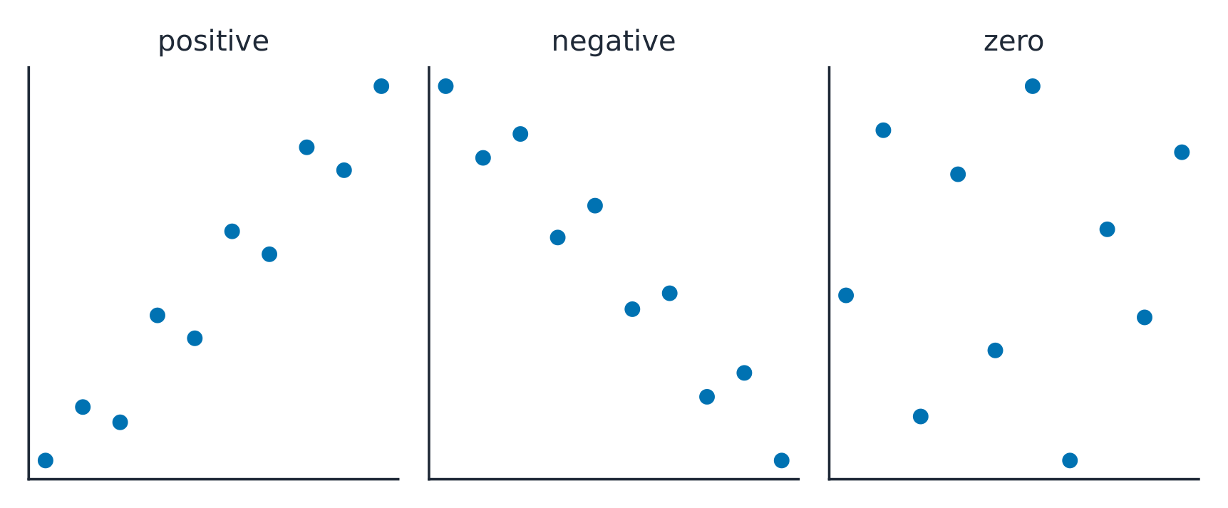
สหสัมพันธ์บวกเพิ่มขึ้นพร้อมกัน; สหสัมพันธ์ลบเคลื่อนที่ในทิศทางตรงข้าม
Explore · ⁨สำรวจ⁩

Strength of a linear relationship · ⁨ความเข้มของความสัมพันธ์เชิงเส้น⁩

Correlation $r$ runs from $-1$ to $1$: near $\pm1$ the points hug a line, near 0 they scatter. Change it and watch the cloud tighten or spread. · ⁨สหสัมพันธ์ $r$Running จาก $-1$ ถึง $1$: ใกล้กับ $\pm1$ จุดจะเกาะติดเส้น, ใกล้ 0 จะกระจายตัว เปลี่ยนมันและดูเมฆแน่นหรือขยายออก⁩

Vocabulary · ⁨คำศัพท์⁩ Train · ⁨ฝึกฝน⁩
English ไทย
correlation coefficient/ˌkɒrɪˈleɪʃn ˌkəʊɪˈfɪʃənt/ สัมประสิทธิ์สหสัมพันธ์
2.6

Linear Regression Models · ⁨โมเดลถดถอยเชิงเส้น⁩

Syllabus · ⁨หลักสูตร⁩
English

Enduring Understanding (DAT-1): Regression models may allow us to predict responses to changes in an explanatory variable.

Learning Objective DAT-1.D: Calculate a predicted response value using a linear regression model. [Skill 2.C]

  • DAT-1.D.1 A simple linear regression model is an equation that uses an explanatory variable, $x$, to predict the response variable, $y$.
  • DAT-1.D.2 The predicted response value, denoted by $\hat{y}$, is calculated as $\hat{y} = a + bx$, where $a$ is the $y$-intercept and $b$ is the slope of the regression line, and $x$ is the value of the explanatory variable.
  • DAT-1.D.3 Extrapolation is predicting a response value using a value for the explanatory variable that is beyond the interval of $x$-values used to determine the regression line. The predicted value is less reliable as an estimate the further we extrapolate.
ไทย

ความเข้าใจที่ยั่งยืน (DAT-1): แบบจำลองการถดถอยอาจช่วยให้เราทำนายผลลัพธ์จากการเปลี่ยนแปลงในตัวแปรอธิบายได้

วัตถุประสงค์การเรียนรู้ DAT-1.D: คำนวณค่าที่คาดการณ์โดยใช้แบบจำลองการถดถอยเชิงเส้น [ทักษะ 2.C]

  • DAT-1.D.1 แบบจำลองการถดถอยเชิงเส้นอย่างง่ายคือสมการที่ใช้ตัวแปรอธิบาย, $x$, เพื่อทำนายตัวแปรตอบสนอง, $y$
  • DAT-1.D.2 ค่าที่คาดการณ์, แทนด้วย $\hat{y}$, คำนวณได้จาก $\hat{y} = a + bx$, โดยที่ $a$ คือจุดตัด $y$-แกน และ $b$ คือความชันของเส้นถดถอย, และ $x$ คือค่าของตัวแปรอธิบาย
  • DAT-1.D.3 การ EXTRAPOLATION คือการทำนายค่าคำตอบโดยใช้ค่าของตัวแปรอธิบายที่อยู่เกินช่วงของค่า $x$ ที่ใช้ในการหาเส้นถดถอย ค่าที่คาดคะเนจะเชื่อถือได้น้อยลงเมื่อเรา extrapolate ไปไกลขึ้น

Source: College Board AP Course and Exam Description · ⁨แหล่งที่มา: คำอธิบายหลักสูตรและข้อสอบ College Board AP⁩

English

The least-squares regression line 最小二乘回归线 predicts the response: $\hat{y}=a+bx$, where $\hat{y}$ is the predicted response. The slope 斜率 $b$ is the predicted change in $y$ per one-unit increase in $x$; the $y$-intercept 截距 $a$ is the predicted $y$ when $x=0$. Interpret both in context and with units – a graded skill. Avoid extrapolation 外推 (predicting far outside the data).

Worked example. A study of hours studied ($x$) and test score ($y$) gives $\hat{y}=20+3x$. The slope means each extra hour of study is associated with a predicted $3$-point increase. A student who studies $5$ hours is predicted to score $\hat{y}=20+3(5)=35$.

ไทย

เส้นถดถอยกำลังน้อยที่สุด (least-squares regression line) ทำนายค่าตอบรับ: $\hat{y}=a+bx$, โดยที่ $\hat{y}$ คือ ค่าตอบรับที่ทำนาย. ความชัน $b$ คือการเปลี่ยนแปลงที่คาดหมายใน $y$ ต่อการเพิ่มขึ้นหนึ่งหน่วยใน $x$; จุดตัดแกน $y$ $a$ คือค่า $y$ ที่คาดหมายเมื่อ $x=0$. ตีความทั้งสอง ในบริบทและมีหน่วย – เป็นทักษะที่ต้องฝึกฝน หลีกเลี่ยง การ экстраโพลเลชัน (การทำนายไกลนอกข้อมูล)

ตัวอย่างวิธีทำ. การศึกษาเกี่ยวกับชั่วโมงเรียน ($x$) และคะแนนทดสอบ ($y$) ได้ $\hat{y}=20+3x$. Slope หมายความว่าทุก额外的小时对应的 predicted increase of $3$ points. นักเรียนที่เรียน $5$ ชั่วโมง会被预测得分为 $\hat{y}=20+3(5)=35$.

Explore · ⁨สำรวจ⁩

Fit a least-squares line · ⁨ปรับเส้นน้อยที่สุดกำลังสอง⁩

A regression line is the best straight-line fit, minimising the squared vertical distances. Its slope predicts how $y$ changes per unit of $x$. · ⁨เส้นถดถอย คือการปรับเส้นตรงที่ดีที่สุด โดยลดระยะทางแนวตั้งกำลังสองลง เส้นนี้ทำนายว่า $y$ จะเปลี่ยนไปเท่าไหร่ต่อหน่วยของ $x$⁩

Vocabulary · ⁨คำศัพท์⁩ Train · ⁨ฝึกฝน⁩
English ไทย
least-squares regression line/liːst skweəz rɪˈɡreʃn laɪn/ เส้นถดถอยกำลังสองน้อยที่สุด
slope/sləʊp/ ความชัน
y-intercept/waɪ ˌɪntəˈsept/ จุดตัดแกน y
extrapolation/ekˈstræpəleɪʃn/ การขยายนอกขอบเขตข้อมูล (extrapolation)
2.7

Residuals · ⁨ค่าคงเหลือ (Residuals)⁩

Syllabus · ⁨หลักสูตร⁩
English

Enduring Understanding (DAT-1): Regression models may allow us to predict responses to changes in an explanatory variable.

Learning Objective DAT-1.E: Represent differences between measured and predicted responses using residual plots. [Skill 2.B]

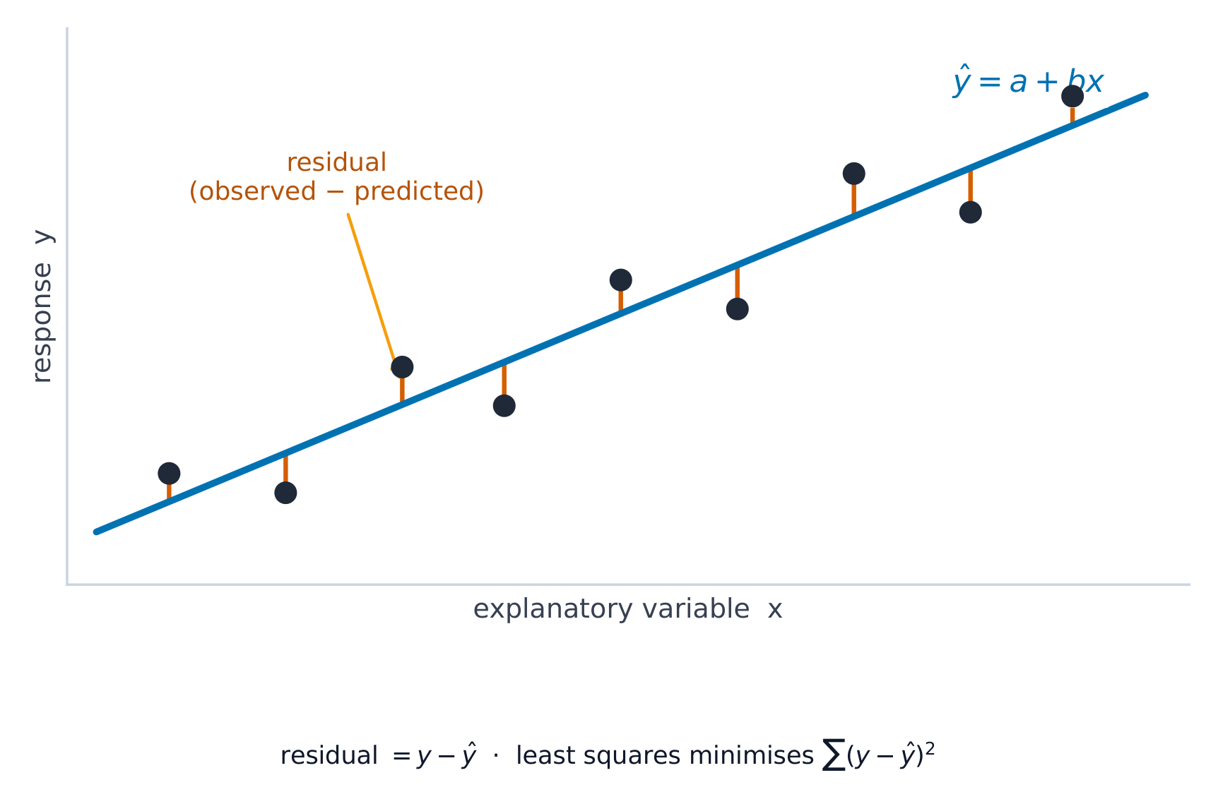
  • DAT-1.E.1 The residual is the difference between the actual value and the predicted value: $\text{residual} = y - \hat{y}$.
  • DAT-1.E.2 A residual plot is a plot of residuals versus explanatory variable values or predicted response values.

Learning Objective DAT-1.F: Describe the form of association of bivariate data using residual plots. [Skill 2.A]

  • DAT-1.F.1 Apparent randomness in a residual plot for a linear model is evidence of a linear form to the association between the variables.
  • DAT-1.F.2 Residual plots can be used to investigate the appropriateness of a selected model.
ไทย

ความเข้าใจที่ยั่งยืน (DAT-1): แบบจำลองการถดถอยอาจช่วยให้เราทำนายผลลัพธ์จากการเปลี่ยนแปลงในตัวแปรอธิบายได้

วัตถุประสงค์การเรียนรู้ DAT-1.E: แสดงความแตกต่างระหว่างค่าที่วัดได้และค่าที่คาดการณ์โดยใช้กราฟค่าคงเหลือ [ทักษะ 2.B]

  • DAT-1.E.1 ค่าคงเหลือคือความแตกต่างระหว่างค่าจริงและค่าที่คาดการณ์: $\text{residual} = y - \hat{y}$
  • DAT-1.E.2 กราฟค่าคงเหลือคือกราฟของค่าคงเหลือเทียบกับค่าของตัวแปรอธิบายหรือค่าที่คาดการณ์ของตัวแปรตอบสนอง

วัตถุประสงค์การเรียนรู้ DAT-1.F: อธิบายรูปแบบของความสัมพันธ์ของข้อมูลเชิงปริมาณคู่โดยใช้กราฟค่าคงเหลือ [ทักษะ 2.A]

  • DAT-1.F.1 ความสุ่มที่ปรากฏในกราฟค่าคงเหลือสำหรับแบบจำลองเชิงเส้นเป็นหลักฐานของรูปแบบเชิงเส้นของความสัมพันธ์ระหว่างตัวแปร
  • DAT-1.F.2 กราฟค่าคงเหลือสามารถใช้เพื่อตรวจสอบความเหมาะสมของแบบจำลองที่เลือกไว้

Source: College Board AP Course and Exam Description · ⁨แหล่งที่มา: คำอธิบายหลักสูตรและข้อสอบ College Board AP⁩

English
Least-squares regression

A residual 残差 is actual minus predicted, $y-\hat{y}$: how far a point sits above (+) or below (−) the line. A residual plot 残差图 graphs residuals against $x$. If it shows no pattern (random scatter), a linear model is appropriate; a curved or fanning pattern means the linear model is a poor fit.

Worked example. Continuing the study above, a student who studied $5$ hours actually scored $40$. The residual is $y-\hat{y}=40-35=+5$: the line under-predicted by $5$ points, so this point sits above the line.

ไทย
การถดถอยกำลังสองน้อยสุด (Least-squares regression)

ค่าคงเหลือ (residual) คือจริงลบด้วยที่คาด, $y-\hat{y}$: ระยะห่างที่จุดอยู่เหนือ (+) หรือใต้ (−) เส้น. กราฟค่าคงเหลือ (residual plot) กราฟค่าคงเหลือเทียบกับ $x$. หากแสดง ไม่มีรูปแบบ (กระจัดกระจายแบบสุ่ม) โมเดลเชิงเส้นเหมาะสม; รูปแบบโค้งหรือแผ่ออกหมายความว่าโมเดลเชิงเส้นไม่พอดี

ตัวอย่างคำนวณ. ต่อเนื่องจากการศึกษาข้างต้น นักเรียนที่เรียน $5$ ชั่วโมง ได้คะแนนจริง $40$. ค่าคงเหลือคือ $y-\hat{y}=40-35=+5$: เส้น ทำนายต่ำกว่า $5$ คะแนน, ดังนั้นจุดนี้อยู่เหนือเส้น

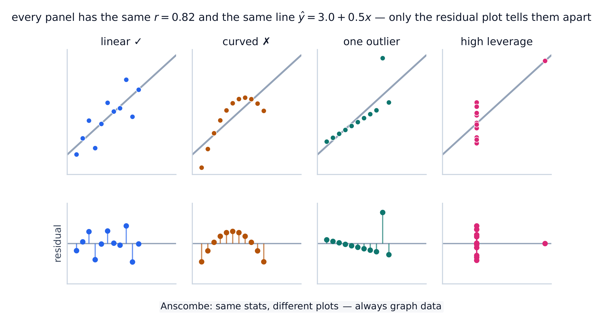
ชุดข้อมูลสี่ชุดที่มี r และเส้นถดถอยเหมือนกันแต่มีรูปทรงต่างกันสี่แบบ
ข้อควรระวังเกี่ยวกับ $r$ และเส้น: ชุดข้อมูลทั้งสี่มี $r=0.82$ และ $\hat{y}=3.0+0.5x$ เหมือนกัน แต่เพียงชุดแรกที่เป็นเชิงเส้นแท้จริง. กราฟกระจายแทบไม่แตกต่างกัน — กราฟค่าคงเหลือ ด้านล่างแต่ละชุดคือสิ่งที่เปิดเผยความโค้ง, ค่าสุดขั้ว, และจุดที่มีน้ำหนักสูง.
Vocabulary · ⁨คำศัพท์⁩ Train · ⁨ฝึกฝน⁩
English ไทย
residual/rɪˈsɪdʒuːəl/ ค่าคงเหลือ
residual plot/rɪˈsɪdʒuːəl plɒt/ แผนภูมิเศษเหลือ (residual plot)
2.8

Least-Squares Regression and Its Fit · ⁨การถดถอยกำลังน้อยที่สุดและการเข้ากันของโมเดล⁩

Syllabus · ⁨หลักสูตร⁩
English

Enduring Understanding (DAT-1): Regression models may allow us to predict responses to changes in an explanatory variable.

Learning Objective DAT-1.G: Estimate parameters for the least-squares regression line model. [Skill 2.C]

  • DAT-1.G.1 The least-squares regression model minimizes the sum of the squares of the residuals and contains the point $(\bar{x}, \bar{y})$.
  • DAT-1.G.2 The slope, $b$, of the regression line can be calculated as $b = r \left( \dfrac{s_y}{s_x} \right)$ where $r$ is the correlation between $x$ and $y$, $s_y$ is the sample standard deviation of the response variable, $y$, and $s_x$ is the sample standard deviation of the explanatory variable, $x$.
  • DAT-1.G.3 Sometimes, the $y$-intercept of the line does not have a logical interpretation in context.
  • DAT-1.G.4 In simple linear regression, $r^2$ is the square of the correlation, $r$. It is also called the coefficient of determination. $r^2$ is the proportion of variation in the response variable that is explained by the explanatory variable in the model.

Learning Objective DAT-1.H: Interpret coefficients for the least-squares regression line model. [Skill 4.B]

  • DAT-1.H.1 The coefficients of the least-squares regression model are the estimated slope and $y$-intercept.
  • DAT-1.H.2 The slope is the amount that the predicted $y$-value changes for every unit increase in $x$.
  • DAT-1.H.3 The $y$-intercept value is the predicted value of the response variable when the explanatory variable is equal to $0$. The formula for the $y$-intercept, $a$, is $a = \bar{y} - b\bar{x}$.
ไทย

ความเข้าใจที่ยั่งยืน (DAT-1): แบบจำลองการถดถอยอาจช่วยให้เราทำนายผลลัพธ์จากการเปลี่ยนแปลงในตัวแปรอธิบายได้

จุดประสงค์การเรียนรู้ DAT-1.G: ประมาณค่าพารามิเตอร์สำหรับโมเดลเส้นถดถอยกำลังน้อยที่สุด [ทักษะ 2.C]

  • DAT-1.G.1 โมเดลถดถอยกำลังน้อยที่สุดจะลดผลรวมของกำลังสองของความคลาดเคลื่อน (residuals) ลงให้ต่ำสุด และมีจุด $(\bar{x}, \bar{y})$ อยู่บนเส้น
  • DAT-1.G.2 ความชัน, $b$, ของเส้นถดถอยสามารถคำนวณได้จาก $b = r \left( \dfrac{s_y}{s_x} \right)$ โดยที่ $r$ คือสัมประสิทธิ์สหสัมพันธ์ระหว่าง $x$ และ $y$, $s_y$ คือส่วนเบี่ยงเบนมาตรฐานของตัวอย่างของตัวแปรตอบรับ, $y$, และ $s_x$ คือส่วนเบี่ยงเบนมาตรฐานของตัวอย่างของตัวแปรอธิบาย, $x$.
  • DAT-1.G.3 บางครั้ง ค่าตัดแกน $y$ ของเส้นอาจไม่มีความหมายในบริบทของปัญหา
  • DAT-1.G.4 ในสมการถดถอยเชิงเส้นอย่างง่าย, $r^2$ คือกำลังสองของสัมประสิทธิ์สหสัมพันธ์, $r$ มันยังเรียกว่าสัมประสิทธิ์การกำหนด $r^2$ เป็นสัดส่วนของความแปรปรวนในตัวแปรตอบรับที่ถูกอธิบายโดยตัวแปรอธิบายในโมเดล

จุดประสงค์การเรียนรู้ DAT-1.H: ตีความสัมประสิทธิ์สำหรับโมเดลเส้นถดถอยกำลังน้อยที่สุด [ทักษะ 4.B]

  • DAT-1.H.1 สัมประสิทธิ์ของโมเดลถดถอยกำลังน้อยที่สุดคือความชันประมาณการและค่าตัดแกน $y$
  • DAT-1.H.2 ความชันคือปริมาณที่ค่า预测 $y$ เปลี่ยนแปลงไปสำหรับทุกหน่วยที่เพิ่มขึ้นของ $x$
  • DAT-1.H.3 ค่าตัดแกน $y$ คือค่า预测ของตัวแปรตอบรับเมื่อตัวแปรอธิบายมีค่าเท่ากับ $0$ สูตรสำหรับค่าตัดแกน $y$, $a$, คือ $a = \bar{y} - b\bar{x}$

Source: College Board AP Course and Exam Description · ⁨แหล่งที่มา: คำอธิบายหลักสูตรและข้อสอบ College Board AP⁩

English

The line minimizes the sum of squared residuals. Its fit is measured by:

  • $s$, the standard deviation of the residuals – the typical prediction error, in the response's units.
  • $r^2$, the coefficient of determination 决定系数 – the proportion of the variation in $y$ that the linear model explains (a value between $0$ and $1$; multiply by $100$ to state it as a percent). Report it in context: "$r^2 = 0.81$ means 81% of the variation in $y$ is explained by the linear relationship with $x$."
ไทย
เส้นกำลังน้อยที่สุดลดผลรวมของค่าคงเหลือยกกำลังสองให้ต่ำสุด

เส้นลดผลรวมของค่าคงเหลือยกกำลังสองให้ต่ำสุด การเข้ากันวัดโดย:

  • $s$, ส่วนเบี่ยงเบนมาตรฐานของค่าคงเหลือ – ความผิดพลาดในการคาดหมายทั่วไป, ในหน่วยของค่าตอบรับ.
  • $r^2$, สัมประสิทธิ์การกำหนด (coefficient of determination) – สัดส่วนของความแปรปรวนใน $y$ ที่โมเดลเชิงเส้นอธิบาย (ค่าระหว่าง $0$ และ $1$; คูณด้วย $100$ เพื่อระบุเป็นเปอร์เซ็นต์). รายงานในบริบท: "$r^2 = 0.81$ หมายถึง 81% ของความแปรปรวนใน $y$ ถูกอธิบายด้วยความสัมพันธ์เชิงเส้นกับ $x$."
Vocabulary · ⁨คำศัพท์⁩ Train · ⁨ฝึกฝน⁩
English ไทย
coefficient of determination/ˌkəʊɪˈfɪʃənt ɒv dɪˌtɜːmɪˈneɪʃn/ สัมประสิทธิ์การกำหนด (coefficient of determination)
2.9

Departures from Linearity · ⁨ความเบี่ยงเบนจากความเป็นเชิงเส้น⁩

Syllabus · ⁨หลักสูตร⁩
English

Enduring Understanding (DAT-1): Regression models may allow us to predict responses to changes in an explanatory variable.

Learning Objective DAT-1.I: Identify influential points in regression. [Skill 2.A]

  • DAT-1.I.1 An outlier in regression is a point that does not follow the general trend shown in the rest of the data and has a large residual when the Least Squares Regression Line (LSRL) is calculated.
  • DAT-1.I.2 A high-leverage point in regression has a substantially larger or smaller $x$-value than the other observations have.
  • DAT-1.I.3 An influential point in regression is any point that, if removed, changes the relationship substantially. Examples include much different slope, $y$-intercept, and/or correlation. Outliers and high leverage points are often influential.

Learning Objective DAT-1.J: Calculate a predicted response using a least-squares regression line for a transformed data set. [Skill 2.C]

  • DAT-1.J.1 Transformations of variables, such as evaluating the natural logarithm of each value of the response variable or squaring each value of the explanatory variable, can be used to create transformed data sets, which may be more linear in form than the untransformed data.
  • DAT-1.J.2 Increased randomness in residual plots after transformation of data and/or movement of $r^2$ to a value closer to 1 offers evidence that the least-squares regression line for the transformed data is a more appropriate model to use to predict responses to the explanatory variable than the regression line for the untransformed data.
ไทย

ความเข้าใจที่ยั่งยืน (DAT-1): แบบจำลองการถดถอยอาจช่วยให้เราทำนายผลลัพธ์จากการเปลี่ยนแปลงในตัวแปรอธิบายได้

จุดประสงค์การเรียนรู้ DAT-1.I: ชนจุดที่มีอิทธิพลในการถดถอย [ทักษะ 2.A]

  • DAT-1.I.1 จุดผิดปกติ (outlier) ในการถดถอยคือจุดที่ไม่สอดคล้องกับแนวโน้มทั่วไปที่แสดงอยู่ในข้อมูลส่วนที่เหลือและมีค่าความคลาดเคลื่อนสูงเมื่อคำนวณเส้นถดถอยกำลังน้อยที่สุด (LSRL)
  • DAT-1.I.2 จุดที่มีอำนาจสูง (high-leverage point) ในการถดถอยมีค่า $x$ ที่แตกต่างกันอย่างมากหรือมากกว่า/น้อยกว่าจุดสังเกตอื่นๆ อย่างชัดเจน
  • DAT-1.I.3 จุดที่มีอิทธิพล (influential point) ในการถดถอยคือจุดใดๆ ที่หากถูกนำออก จะทำให้ความสัมพันธ์เปลี่ยนแปลงไปอย่างมาก ตัวอย่างเช่น ความชัน, ค่าตัดแกน $y$, และ/หรือ สัมประสิทธิ์สหสัมพันธ์ที่แตกต่างกันมาก จุดผิดปกติและจุดที่มีอำนาจสูงมักจะมีอิทธิพล

จุดประสงค์การเรียนรู้ DAT-1.J: คำนวณค่า predicted response โดยใช้เส้นถดถอยกำลังน้อยที่สุดสำหรับชุดข้อมูลที่แปลงแล้ว [ทักษะ 2.C]

  • DAT-1.J.1 การแปลงตัวแปร เช่น การหาค่าลอการิทึมธรรมชาติของแต่ละค่าของตัวแปรตอบรับ หรือการยกกำลังสองของแต่ละค่าของตัวแปรอธิบาย สามารถใช้เพื่อสร้างชุดข้อมูลที่แปลงแล้ว ซึ่งอาจมีความเป็นเชิงเส้นมากกว่าข้อมูลที่ไม่ได้แปลง
  • DAT-1.J.2 ความสุ่มที่เพิ่มขึ้นในกราฟความคลาดเคลื่อนหลังการแปลงข้อมูลและ/หรือการเคลื่อนย้าย $r^2$ ไปสู่ค่าที่ใกล้ 1 มากขึ้น เป็นหลักฐานว่าเส้นถดถอยกำลังน้อยที่สุดสำหรับข้อมูลที่ได้แปลงแล้วเป็นโมเดลที่เหมาะสมกว่าในการ predict responses ต่อตัวแปรอธิบาย เมื่อเทียบกับเส้นถดถอยสำหรับข้อมูลที่ไม่ได้แปลง

Source: College Board AP Course and Exam Description · ⁨แหล่งที่มา: คำอธิบายหลักสูตรและข้อสอบ College Board AP⁩

English

Some points strongly affect the line. A high-leverage 高杠杆 point has an extreme $x$-value; an influential 有影响的 point noticeably changes the slope or $r$ when removed; an outlier here is a point with a large residual. When the pattern is curved, transform a variable (e.g. take a log) to straighten it, then fit a line to the transformed data.

ไทย

บางจุดส่งผลต่อเส้นอย่างมาก จุด น้ำหนักสูง (high-leverage) มีค่า $x$ ที่สุดขั้ว; จุด มีอิทธิพล (influential) เปลี่ยนความชันหรือ $r$ อย่างชัดเจนเมื่อถูกเอาออก; ค่าสุดขั้ว (outlier)在这里 คือจุดที่มีค่าคงเหลือใหญ่. เมื่อรูปแบบเป็นโค้ง ให้ แปลง ตัวแปร (เช่นTaking a log) เพื่อให้เป็นเส้นตรง แล้วปรับเส้นเข้ากับข้อมูลที่แปลงแล้ว

Vocabulary · ⁨คำศัพท์⁩ Train · ⁨ฝึกฝน⁩
English ไทย
high-leverage/haɪ ˈliːvərɪdʒ/ จุดที่มีอิทธิพลสูง (high-leverage)
influential/ˌɪnfluːˈenʃl/ มีอิทธิพล (influential)
2.9

Exam tips · ⁨ข้อแนะนำสำหรับการสอบ⁩

English
  • On a scatterplot describe direction, form, strength, and outliers; $r$ ranges $-1$ to $1$.
  • Correlation is not causation — a lurking variable can drive both.
  • Interpret the slope of the least-squares line in context ("per one unit of $x$, predicted $y$ changes by $b$").
  • Check a residual plot: no pattern means a line fits; a curve means it does not. Avoid extrapolation.
  • $r^2$ is the fraction of variation in $y$ explained by the model.
ไทย
  • บนกราฟกระจาย อธิบาย ทิศทาง, รูปแบบ, ความเข้ม, และค่าสุดขั้ว; $r$ มีช่วง $-1$ ถึง $1$.
  • สหสัมพันธ์ไม่ใช่สาเหตุ – ตัวแปรแฝงอาจขับเคลื่อนทั้งสองอย่าง
  • ตีความความชันของเส้นกำลังน้อยที่สุดในบริบท ("ต่อหนึ่งหน่วยของ $x$, ค่า $y$ ที่คาดเปลี่ยนไป $b$").
  • ตรวจสอบ กราฟค่าคงเหลือ: ไม่มีแปลว่าเส้นเข้ากัน; เป็นโค้งแปลว่าไม่เข้ากัน. หลีกเลี่ยงการ ekstrapolation
  • $r^2$ คือสัดส่วนของความแปรปรวนใน $y$ ที่โมเดลอธิบายได้

Interactive lessons on this topic · ⁨บทเรียนเชิงโต้ตอบสำหรับหัวข้อนี้⁩

Work through it step by step, with instant-check exercises. · ⁨ทำทีละขั้นตอน พร้อมแบบฝึกหัดตรวจสอบผลทันที⁩

Past Papers · ⁨ข้อสอบย้อนหลัง⁩

More topics in AP Statistics · ⁨หัวข้อเพิ่มเติมใน AP Statistics⁩

Log in or create account · ⁨เข้าสู่ระบบหรือสร้างบัญชี⁩

IGCSE, A-Level & AP