Skip to content · ⁨ข้ามไปยังเนื้อหา⁩
Subjects · ⁨รายวิชา⁩

AP Statistics

Tips · ⁨เคล็ดลับ⁩

AP Statistics ครอบคลุม การสำรวจข้อมูล, การสุ่มตัวอย่างและการออกแบบการทดลอง, ความน่าจะเป็นและตัวแปรสุ่ม, การกระจายตัวของค่าเฉลี่ยจากตัวอย่าง และ การอนุมาน — ช่วงความเชื่อมั่นและการทดสอบนัยสำคัญ มีพีชคณิตน้อยมาก ความยากอยู่ที่ การ表述ความไม่แน่นอนอย่างถูกต้อง

คำตอบทุกข้อเกี่ยวกับการอนุมานต้องมีสี่ส่วน: ระบุชื่อขั้นตอน, ตรวจสอบเงื่อนไข, คำนวณ และ สรุปโดยเชื่อมโยงกับบริบทพร้อมกล่าวถึงสมมติฐานทางเลือก เกณฑ์ให้คะแนนประเมินทั้งสี่ส่วน ดังนั้นการได้ค่า p ที่ถูกต้องเพียงอย่างเดียวแต่ขาดส่วนอื่นจะได้คะแนนต่ำ

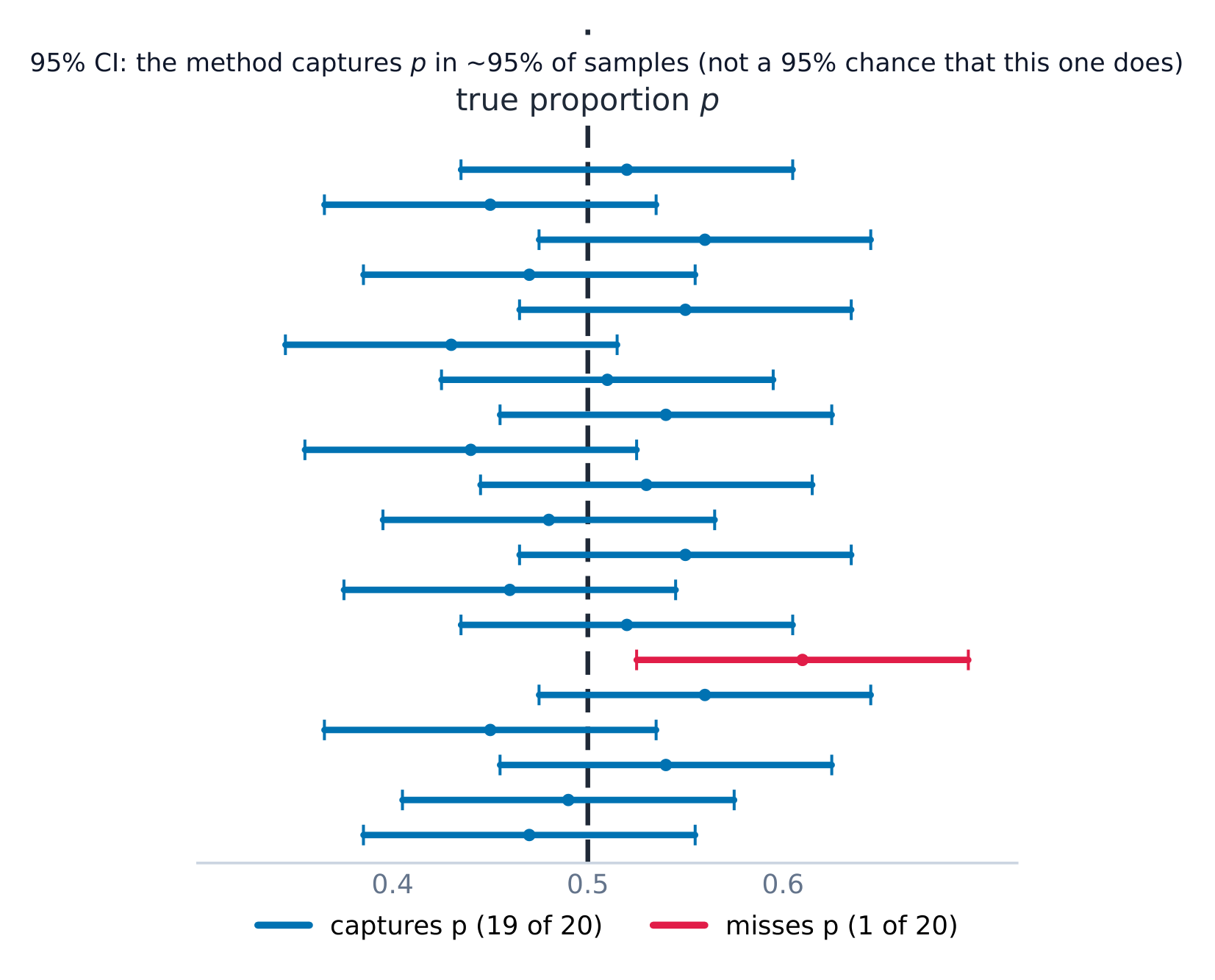
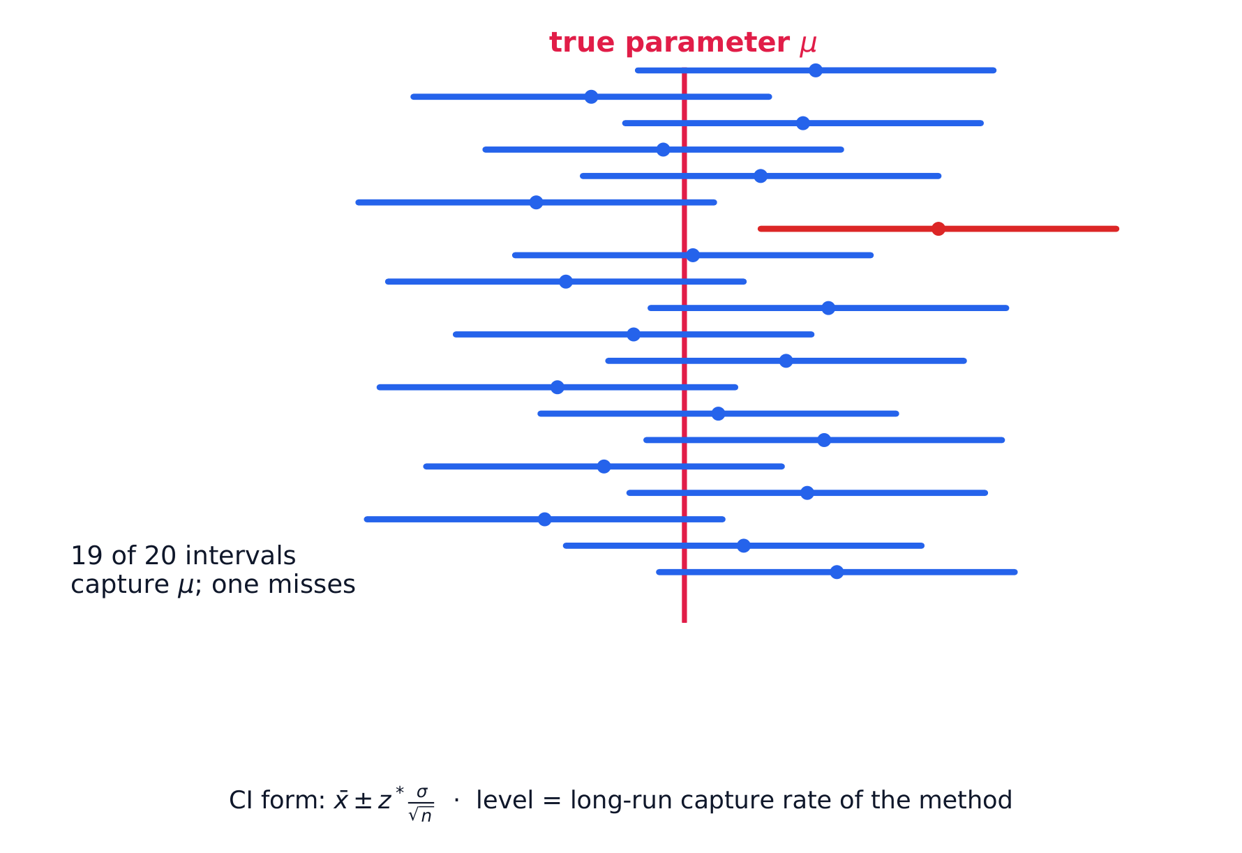
ภาษาถูกประเมินด้วย คำว่า "เราปฏิเสธ H₀" ไม่ใช่ "เราพิสูจน์ H₁"; ช่วงความเชื่อมั่นเกี่ยวกับ พฤติกรรมในระยะยาวของวิธีการ ไม่ใช่ความน่าจะเป็นที่ช่วงนั้นจะรวมพารามิเตอร์ไว้ การแยกแยะเหล่านี้กำหนดคะแนน

หมายเหตุนี้ครอบคลุมทั้งเก้าหน่วย โดยแต่ละขั้นตอนการอนุมานแสดงทีละขั้นตอน FRQs ที่เผยแพร่แล้วอยู่ในห้องสมุดวิชาสถิติให้คะแนนสำหรับ การระบุเงื่อนไขและการตีความในบริบท ดังนั้นทุกตัวอย่างคำตอบจะระบุเงื่อนไขก่อนดำเนินการทดสอบ

  • 1

    Exploring One-Variable Data · ⁨การสำรวจข้อมูลตัวแปรเดียว⁩

    Watch lesson · ⁨ดูบทเรียน⁩
    1.1

    Introducing Statistics: What Can We Learn from Data? · ⁨แนะนำสถิติ: เราเรียนรู้จากข้อมูลได้อย่างไร?⁩

    Syllabus · ⁨หลักสูตร⁩
    English

    Enduring Understanding (VAR-1): Given that variation may be random or not, conclusions are uncertain.

    Learning Objective VAR-1.A: Identify questions to be answered, based on variation in one-variable data. [Skill 1.A]

    • VAR-1.A.1 Numbers may convey meaningful information, when placed in context.
    ไทย

    ความเข้าใจที่ยั่งยืน (VAR-1): เนื่องจากความแปรปรวนอาจเป็นแบบสุ่มหรือไม่ ดังนั้นข้อสรุปจึงมีความไม่แน่นอน

    จุดประสงค์การเรียนรู้ VAR-1.A: ระบุคำถามที่ต้องการตอบ โดยอ้างอิงจากความแปรปรวนในข้อมูลหนึ่งตัวแปร [ทักษะ 1.A]

    • VAR-1.A.1 ตัวเลขอาจส่งผ่านข้อมูลที่มีความหมาย เมื่อถูก đặtอยู่ในบริบท

    Source: College Board AP Course and Exam Description · ⁨แหล่งที่มา: คำอธิบายหลักสูตรและข้อสอบ College Board AP⁩

    English

    Statistics 统计学 is the science of learning from data 数据 – numbers or labels collected from the real world. Data vary, so we describe patterns and account for the variation 变异 rather than expecting every value to match. A statistical question anticipates an answer based on data that vary.

    Two distinctions run through the whole course. A parameter 参数 is a numerical summary of a whole population; a statistic 统计量 is a numerical summary of a sample - we use the statistic to estimate the parameter we cannot measure directly. And descriptive statistics 描述统计 only summarise the data set in hand, while inferential statistics 推断统计 use a sample to make and test claims about the larger population.

    ไทย

    สถิติ คือวิทยาศาสตร์แห่งการเรียนรู้จาก ข้อมูล – ตัวเลขหรือฉลากที่เก็บมาจากโลกจริง ข้อมูลมีความแปรปรวน ดังนั้นเราจึงอธิบายรูปแบบและคำนึงถึง ความแปรปรวน แทนที่จะคาดหวังให้ทุกค่าตรงกัน คำถามทางสถิติคาดการณ์คำตอบโดยอิงจากข้อมูลที่มีการเปลี่ยนแปลง

    มีความแตกต่างสองประการ贯穿整个课程。 Parameter คือสรุปตัวเลขของ ประชากร ทั้งหมด; Statistic คือสรุปตัวเลขของ ตัวอย่าง – เราใช้ statistic เพื่อประมาณ parameter ที่เราไม่สามารถวัดโดยตรงได้ และ descriptive statistics สรุปเฉพาะชุดข้อมูลที่มีอยู่เท่านั้น ในขณะที่ inferential statistics ใช้ตัวอย่างเพื่อสร้างและทดสอบ claims เกี่ยวกับประชากรขนาดใหญ่กว่า

    Vocabulary · ⁨คำศัพท์⁩ Train · ⁨ฝึกฝน⁩
    English ไทย
    Statistics/stəˈtɪstɪks/ สถิติ
    data/ˈdeɪtə/ ข้อมูล (data)
    variation/ˌveərɪˈeɪʃn/ ความหลากหลาย (Variation)
    parameter/pəˈræmɪtə/ พารามิเตอร์
    statistic/stəˈtɪstɪk/ ค่าสถิติ
    descriptive statistics/dɪˈskrɪptɪv stəˈtɪstɪks/ สถิติเชิงพรรณนา
    inferential statistics/ɪnfəˈrenʃl stəˈtɪstɪks/ สถิติเชิงอนุมาน
    variable/ˈveərɪəbl/ ตัวแปร
    1.2

    The Language of Variation: Variables · ⁨ภาษาของความแปรปรวน: ตัวแปร⁩

    Syllabus · ⁨หลักสูตร⁩
    English

    Enduring Understanding (VAR-1): Given that variation may be random or not, conclusions are uncertain.

    Learning Objective VAR-1.B: Identify variables in a set of data. [Skill 2.A]

    • VAR-1.B.1 A variable is a characteristic that changes from one individual to another.

    Learning Objective VAR-1.C: Classify types of variables. [Skill 2.A]

    • VAR-1.C.1 A categorical variable takes on values that are category names or group labels.
    • VAR-1.C.2 A quantitative variable is one that takes on numerical values for a measured or counted quantity.
      • Illustrative examples for VAR-1.C:
        • Categorical variables:
          • Dominant hand
          • Age group (young or old)
          • Highest degree earned
        • Quantitative variables:
          • Age of a structure
          • Height of a child
          • Concentration of a sample
    ไทย

    ความเข้าใจที่ยั่งยืน (VAR-1): เนื่องจากความแปรปรวนอาจเป็นแบบสุ่มหรือไม่ ดังนั้นข้อสรุปจึงมีความไม่แน่นอน

    จุดประสงค์การเรียนรู้ VAR-1.B: ระบุตัวแปรในชุดข้อมูล [ทักษะ 2.A]

    • VAR-1.B.1 ตัวแปรคือลักษณะที่เปลี่ยนแปลงจากบุคคลหนึ่งไปยังอีกบุคคลหนึ่ง

    จุดประสงค์การเรียนรู้ VAR-1.C: จำแนกประเภทของตัวแปร [ทักษะ 2.A]

    • VAR-1.C.1 ตัวแปรเชิงหมวดหมู่รับค่าที่เป็นชื่อหมวดหมู่หรือฉลากกลุ่ม
    • VAR-1.C.2 ตัวแปรเชิงปริมาณคือตัวแปรที่รับค่าตัวเลขสำหรับปริมาณที่วัดหรือนับ
      • ตัวอย่างประกอบสำหรับ VAR-1.C:
        • ตัวแปรเชิงหมวดหมู่:
          • มือที่ถนัด
          • กลุ่มอายุ (เด็กหรือผู้สูงอายุ)
          • ระดับการศึกษาสูงสุดที่ได้รับ
        • ตัวแปรเชิงปริมาณ:
          • อายุของโครงสร้าง
          • ส่วนสูงของเด็ก
          • ความเข้มข้นของตัวอย่าง

    Source: College Board AP Course and Exam Description · ⁨แหล่งที่มา: คำอธิบายหลักสูตรและข้อสอบ College Board AP⁩

    English

    A variable 变量 is a characteristic that can differ between individuals. Two kinds:

    • Categorical 分类 (qualitative): values are labels/groups (eye colour, brand).
    • Quantitative 定量: values are numbers you can do arithmetic on (height, age). Quantitative variables are discrete (countable) or continuous (measured).

    Choosing the right graph and summary depends on which kind you have.

    ไทย

    ตัวแปร คือคุณลักษณะที่แตกต่างกันระหว่างบุคคลได้ มีสองประเภท:

    • Categorical (qualitative): ค่าคือฉลาก/กลุ่ม (สีตา, แบรนด์)
    • Quantitative: ค่าคือตัวเลขที่สามารถคำนวณทางคณิตศาสตร์ได้ (ส่วนสูง, อายุ) ตัวแปร quantitative เป็น discrete (นับได้) หรือ continuous (วัดได้)

    การเลือกกราฟและสรุปที่เหมาะสมขึ้นอยู่กับว่าคุณมีประเภทใด

    Explore · ⁨สำรวจ⁩

    Categorical or quantitative? · ⁨Categorical หรือ quantitative?⁩

    Every variable is either categorical (it labels each unit with a group) or quantitative (a measured number you can average). Which kind it is decides the graphs and summaries you are allowed to use. · ⁨ตัวแปรทุกตัวเป็นeither ประเภท (ซึ่งระบุกลุ่มให้กับหน่วย) หรือ ปริมาณ (ตัวเลขที่วัดได้ที่คุณสามารถหาค่าเฉลี่ยได้) ประเภทไหนจะเป็นตัวกำหนดกราฟและสรุปผลที่คุณสามารถใช้ได้⁩

    Vocabulary · ⁨คำศัพท์⁩ Train · ⁨ฝึกฝน⁩
    English ไทย
    Categorical/ˌkætɪˈɡɒrɪkl/ ประเภท
    Quantitative/ˈkwɒntɪteɪtɪv/ ปริมาณ
    1.3

    Representing a Categorical Variable with Tables · ⁨แสดงตัวแปร categorical ด้วยตาราง⁩

    Syllabus · ⁨หลักสูตร⁩
    English

    Enduring Understanding (UNC-1): Graphical representations and statistics allow us to identify and represent key features of data.

    Learning Objective UNC-1.A: Represent categorical data using frequency or relative frequency tables. [Skill 2.B]

    • UNC-1.A.1 A frequency table gives the number of cases falling into each category. A relative frequency table gives the proportion of cases falling into each category.

    Learning Objective UNC-1.B: Describe categorical data represented in frequency or relative tables. [Skill 2.A]

    • UNC-1.B.1 Percentages, relative frequencies, and rates all provide the same information as proportions.
    • UNC-1.B.2 Counts and relative frequencies of categorical data reveal information that can be used to justify claims about the data in context.
    ไทย

    ความเข้าใจที่ยั่งยืน (UNC-1): กราฟและสถิติช่วยให้เราระบุและแสดงคุณลักษณะสำคัญของข้อมูลได้

    วัตถุประสงค์การเรียนรู้ UNC-1.A: แสดงข้อมูลเชิงหมวดหมู่โดยใช้ตารางความถี่หรือความถี่สัมพัทธ์ [ทักษะ 2.B]

    • UNC-1.A.1 ตารางความถี่แสดงจำนวนกรณีในแต่ละหมวดหมู่ ตารางความถี่สัมพัทธ์แสดงสัดส่วนของกรณีในแต่ละหมวดหมู่

    วัตถุประสงค์การเรียนรู้ UNC-1.B: อธิบายข้อมูลเชิงหมวดหมู่ที่แสดงในตารางความถี่หรือตารางความถี่สัมพัทธ์ [ทักษะ 2.A]

    • UNC-1.B.1 เปอร์เซ็นต์ ความถี่สัมพัทธ์ และอัตรา ล้วนให้ข้อมูลที่เหมือนกันกับสัดส่วน
    • UNC-1.B.2 จำนวนและความถี่สัมพัทธ์ของข้อมูลเชิงหมวดหมู่เปิดเผยข้อมูลที่สามารถใช้เพื่อสนับสนุนข้ออ้างเกี่ยวกับข้อมูลในบริบทนั้นๆ

    Source: College Board AP Course and Exam Description · ⁨แหล่งที่มา: คำอธิบายหลักสูตรและข้อสอบ College Board AP⁩

    English

    A frequency table 频数表 lists each category's count (frequency); a relative frequency 相对频率 table lists each category's proportion 比例 (count ÷ total). Relative frequencies let you compare groups of different sizes fairly.

    ไทย

    Frequency table列出每个类别的 count (frequency); Relative frequency table列出每个类别的 proportion (count ÷ total). Relative frequencies ช่วยให้คุณเปรียบเทียบกลุ่มที่มีขนาดต่างกันได้อย่างยุติธรรม

    Vocabulary · ⁨คำศัพท์⁩ Train · ⁨ฝึกฝน⁩
    English ไทย
    frequency table/ˈfriːkwənsi ˈteɪbl/ ตารางความถี่ (frequency table)
    relative frequency/ˈrelətɪv ˈfriːkwənsi/ ความถี่สัมพัทธ์
    proportion/prəˈpɔːʃn/ proportion
    1.4

    Representing a Categorical Variable with Graphs · ⁨แสดงตัวแปร categorical ด้วยกราฟ⁩

    Syllabus · ⁨หลักสูตร⁩
    English

    Enduring Understanding (UNC-1): Graphical representations and statistics allow us to identify and represent key features of data.

    Learning Objective UNC-1.C: Represent categorical data graphically. [Skill 2.B]

    • UNC-1.C.1 Bar charts (or bar graphs) are used to display frequencies (counts) or relative frequencies (proportions) for categorical data.
    • UNC-1.C.2 The height or length of each bar in a bar graph corresponds to either the number or proportion of observations falling within each category.
    • UNC-1.C.3 There are many additional ways to represent frequencies (counts) or relative frequencies (proportions) for categorical data.

    Learning Objective UNC-1.D: Describe categorical data represented graphically. [Skill 2.A]

    • UNC-1.D.1 Graphical representations of a categorical variable reveal information that can be used to justify claims about the data in context.

    Learning Objective UNC-1.E: Compare multiple sets of categorical data. [Skill 2.D]

    • UNC-1.E.1 Frequency tables, bar graphs, or other representations can be used to compare two or more data sets in terms of the same categorical variable.
    ไทย

    ความเข้าใจที่ยั่งยืน (UNC-1): กราฟและสถิติช่วยให้เราระบุและแสดงคุณลักษณะสำคัญของข้อมูลได้

    วัตถุประสงค์การเรียนรู้ UNC-1.C: แสดงข้อมูลเชิงหมวดหมู่ด้วยกราฟ [ทักษะ 2.B]

    • UNC-1.C.1 แผนภูมิแท่ง (หรือกราฟแท่ง) ใช้แสดงความถี่ (จำนวน) หรือความถี่สัมพัทธ์ (สัดส่วน) สำหรับข้อมูลเชิงหมวดหมู่
    • UNC-1.C.2 ความสูงหรือความยาวของแต่ละแท่งในแผนภูมิแท่งสอดคล้องกับจำนวนหรือสัดส่วนของการสังเกตที่ตกอยู่ในแต่ละหมวดหมู่
    • UNC-1.C.3 ยังมีวิธีการเพิ่มเติมอีกมากมายในการแสดงความถี่ (จำนวน) หรือความถี่สัมพัทธ์ (สัดส่วน) สำหรับข้อมูลเชิงหมวดหมู่

    วัตถุประสงค์การเรียนรู้ UNC-1.D: อธิบายข้อมูลเชิงหมวดหมู่ที่แสดงด้วยกราฟ [ทักษะ 2.A]

    • UNC-1.D.1 การแสดงผลด้วยกราฟของตัวแปรเชิงหมวดหมู่เปิดเผยข้อมูลที่สามารถใช้เพื่อสนับสนุนข้ออ้างเกี่ยวกับข้อมูลในบริบทนั้นๆ

    วัตถุประสงค์การเรียนรู้ UNC-1.E: เปรียบเทียบชุดข้อมูลเชิงหมวดหมู่หลายชุด [ทักษะ 2.D]

    • UNC-1.E.1 ตารางความถี่ แผนภูมิแท่ง หรือการแสดงผลอื่นๆ สามารถใช้เพื่อเปรียบเทียบชุดข้อมูลสองชุดขึ้นไปใน terms ของตัวแปรเชิงหมวดหมู่เดียวกัน

    Source: College Board AP Course and Exam Description · ⁨แหล่งที่มา: คำอธิบายหลักสูตรและข้อสอบ College Board AP⁩

    English

    Bar charts 条形图 show the count or proportion of each category as separated bars; a pie chart shows each category's share of the whole. The bar heights (or slices) let you compare categories at a glance. Bars may be ordered by size or by a natural category order.

    ไทย

    Bar charts แสดง count หรือ proportion ของแต่ละ category เป็นแท่งแยก; Pie chart แสดงสัดส่วนของแต่ละ category ของทั้งหมด ความสูงของแท่ง (หรือชิ้นส่วน) ช่วยให้คุณเปรียบเทียบ categories ได้ทันที แท่งอาจเรียงตามขนาดหรือตามลำดับ category ตามธรรมชาติ

    Explore · ⁨สำรวจ⁩

    Show a categorical variable as a pie chart · ⁨แสดงตัวแปรประเภทด้วยแผนภูมิวงกลม⁩

    A pie chart turns each category's share of the whole into a slice: a bigger share is a bigger slice, and every slice together makes 100%. It is a picture of a relative-frequency table. · ⁨แผนภูมิวงกลม แปลงสัดส่วนของแต่ละหมวดหมู่ของทั้งหมดให้เป็นชิ้นส่วน: สัดส่วนที่ใหญ่ขึ้นคือชิ้นส่วนที่ใหญ่ขึ้น และทุกชิ้นส่วนรวมกันเป็น 100% มันคือภาพของตาราง ความถี่สัมพัทธ์⁩

    Vocabulary · ⁨คำศัพท์⁩ Train · ⁨ฝึกฝน⁩
    English ไทย
    Bar charts/bɑː tʃɑːts/ แผนภูมิแท่ง
    1.5

    Representing a Quantitative Variable with Graphs · ⁨แสดงตัวแปร quantitative ด้วยกราฟ⁩

    Syllabus · ⁨หลักสูตร⁩
    English

    Enduring Understanding (UNC-1): Graphical representations and statistics allow us to identify and represent key features of data.

    Learning Objective UNC-1.F: Classify types of quantitative variables. [Skill 2.A]

    • UNC-1.F.1 A discrete variable can take on a countable number of values. The number of values may be finite or countably infinite, as with the counting numbers.
    • UNC-1.F.2 A continuous variable can take on infinitely many values, but those values cannot be counted. No matter how small the interval between two values of a continuous variable, it is always possible to determine another value between them.
      • Illustrative examples for UNC-1.F:
        • A discrete variable:
          • Number of students in a class
        • A continuous variable:
          • Height of a child

    Learning Objective UNC-1.G: Represent quantitative data graphically. [Skill 2.B]

    • UNC-1.G.1 In a histogram, the height of each bar shows the number or proportion of observations that fall within the interval corresponding to that bar. Altering the interval widths can change the appearance of the histogram.
    • UNC-1.G.2 In a stem and leaf plot, each data value is split into a "stem" (the first digit or digits) and a "leaf" (usually the last digit).
    • UNC-1.G.3 A dotplot represents each observation by a dot, with the position on the horizontal axis corresponding to the data value of that observation, with nearly identical values stacked on top of each other.
    • UNC-1.G.4 A cumulative graph represents the number or proportion of a data set less than or equal to a given number.
    • UNC-1.G.5 There are many additional ways to graphically represent distributions of quantitative data.
    ไทย

    ความเข้าใจที่ยั่งยืน (UNC-1): กราฟและสถิติช่วยให้เราระบุและแสดงคุณลักษณะสำคัญของข้อมูลได้

    วัตถุประสงค์การเรียนรู้ UNC-1.F: จำแนกประเภทของตัวแปรเชิงปริมาณ [ทักษะ 2.A]

    • UNC-1.F.1 ตัวแปรแบบไม่ต่อเนื่องสามารถมีค่าจำนวนนับได้ จำนวนค่าอาจเป็นจำกัดหรือนับได้ไม่สิ้นสุด เช่นเดียวกับจำนวนนับ
    • UNC-1.F.2 ตัวแปรแบบต่อเนื่องสามารถมีค่าได้ไม่จำกัด แต่ค่าเหล่านั้นไม่สามารถนับได้ ไม่ว่าช่วงระหว่างค่าสองค่าของตัวแปรแบบต่อเนื่องจะเล็กเพียงใด ก็ยังคงสามารถหาค่าอื่นระหว่างสองค่านั้นได้เสมอ
      • ตัวอย่างประกอบสำหรับ UNC-1.F:
        • ตัวแปรแบบไม่ต่อเนื่อง:
          • จำนวนนักเรียนในห้องเรียน
        • ตัวแปรแบบต่อเนื่อง:
          • ส่วนสูงของเด็ก

    วัตถุประสงค์การเรียนรู้ UNC-1.G: แสดงข้อมูลเชิงปริมาณด้วยกราฟ [ทักษะ 2.B]

    • UNC-1.G.1 ในฮิสโตแกรม ความสูงของแต่ละแท่งแสดงจำนวนหรือสัดส่วนของการสังเกตที่ตกในช่วงที่ตรงกับแท่งนั้น การปรับความกว้างของช่วงสามารถเปลี่ยนรูปลักษณ์ของฮิสโตแกรมได้
    • UNC-1.G.2 ในแผนภูมิก้านและใบ ข้อมูลแต่ละค่าจะถูกแบ่งเป็น "ก้าน" (หลักแรกหรือหลักแรกๆ) และ "ใบ" (มักจะเป็นหลักสุดท้าย)
    • UNC-1.G.3 แผนภูมิจุดแสดงการสังเกตแต่ละค่าด้วยจุด โดยตำแหน่งบนแกนแนวนอนสอดคล้องกับค่าข้อมูลของการสังเกตนั้น โดยมีค่าที่ใกล้เคียงกันมากซ้อนทับกัน
    • UNC-1.G.4 กราฟสะสมแสดงจำนวนหรือสัดส่วนของชุดข้อมูลที่มีค่าน้อยกว่าหรือเท่ากับค่าที่กำหนด
    • UNC-1.G.5 ยังมีวิธีการเพิ่มเติมอีกมากมายในการแสดงผลด้วยการกระจายตัวของข้อมูลเชิงปริมาณ

    Source: College Board AP Course and Exam Description · ⁨แหล่งที่มา: คำอธิบายหลักสูตรและข้อสอบ College Board AP⁩

    English

    For numbers, use a dotplot 点图, stem-and-leaf plot 茎叶图, or histogram 直方图 (bars over value intervals called bins). These show the distribution 分布 – how the values spread out. A histogram's bin width changes the picture, so choose it to reveal the shape.

    ไทย

    สำหรับตัวเลข ใช้ dotplot, stem-and-leaf plot, หรือ histogram (แท่งเหนือช่วงค่าที่เรียกว่า bins). เหล่านี้แสดง distribution – cáchที่ values กระจายออก Width ของ histogram เปลี่ยนภาพดังนั้นเลือกมันเพื่อ reveal的形状

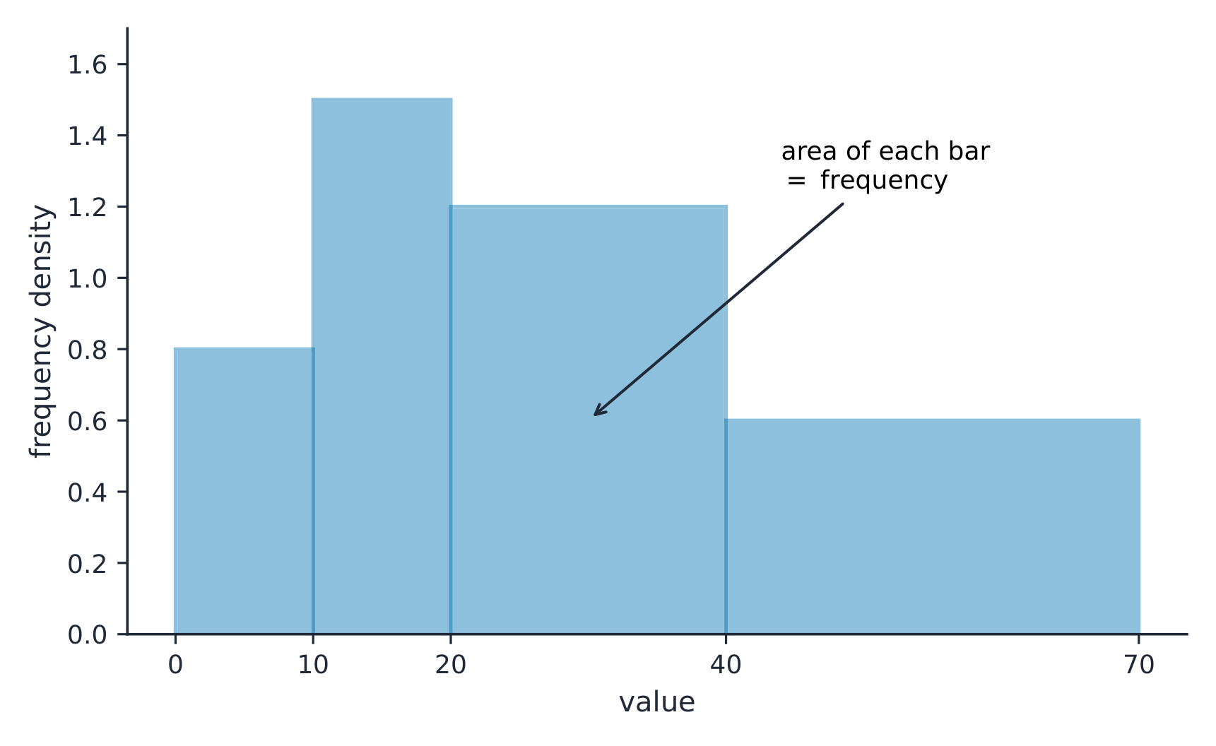
    บนฮิสโตแกรมที่มีช่วงข้อมูลไม่เท่ากัน พื้นที่ของแท่งคือความถี่
    บนฮิสโตแกรมที่มีช่วงข้อมูลไม่เท่ากัน พื้นที่ของแท่งคือความถี่
    Explore · ⁨สำรวจ⁩

    Explore how bin width shapes a histogram · ⁨สำรวจว่าขนาดvron (bin width) ก่อรูปฮิสโตแกรมอย่างไร⁩

    A histogram groups data into equal-width bins and draws a bar over each. Change the bins and notice how the same data can look jagged (too narrow) or smooth (too wide) — the shape is a choice. · ⁨ฮิสโตแกรม จัดกลุ่มข้อมูลลงใน vron ที่มีความกว้างเท่ากันแล้ววาดแท่งบนแต่ละvron เปลี่ยนvronและสังเกตว่าข้อมูลชุดเดียวกันอาจดู หยาบ (แคบเกินไป) หรือ เรียบ (กว้างเกินไป) — รูปทรงเป็นทางเลือก⁩

    Vocabulary · ⁨คำศัพท์⁩ Train · ⁨ฝึกฝน⁩
    English ไทย
    dotplot/ˈdɒtplɒt/ แผนภูมิจุด (dotplot)
    stem-and-leaf plot/stem ænd liːf plɒt/ แผนภูมิก้านและใบ (stem-and-leaf plot)
    histogram/ˈhɪstəɡræm/ ฮิสโตแกรม
    distribution/ˌdɪstrɪˈbjuːʃn/ การกระจาย
    1.6

    Describing the Distribution of a Quantitative Variable · ⁨อธิบาย distribution ของตัวแปร quantitative⁩

    Syllabus · ⁨หลักสูตร⁩
    English

    Enduring Understanding (UNC-1): Graphical representations and statistics allow us to identify and represent key features of data.

    Learning Objective UNC-1.H: Describe the characteristics of quantitative data distributions. [Skill 2.A]

    • UNC-1.H.1 Descriptions of the distribution of quantitative data include shape, center, and variability (spread), as well as any unusual features such as outliers, gaps, clusters, or multiple peaks.
    • UNC-1.H.2 Outliers for one-variable data are data points that are unusually small or large relative to the rest of the data.
    • UNC-1.H.3 A distribution is skewed to the right (positive skew) if the right tail is longer than the left. A distribution is skewed to the left (negative skew) if the left tail is longer than the right. A distribution is symmetric if the left half is the mirror image of the right half.
    • UNC-1.H.4 Univariate graphs with one main peak are known as unimodal. Graphs with two prominent peaks are bimodal. A graph where each bar height is approximately the same (no prominent peaks) is approximately uniform.
    • UNC-1.H.5 A gap is a region of a distribution between two data values where there are no observed data.
    • UNC-1.H.6 Clusters are concentrations of data usually separated by gaps.
    • UNC-1.H.7 Descriptive statistics does not attribute properties of a data set to a larger population, but may provide the basis for conjectures for subsequent testing.
    ไทย

    ความเข้าใจที่ยั่งยืน (UNC-1): กราฟและสถิติช่วยให้เราระบุและแสดงคุณลักษณะสำคัญของข้อมูลได้

    วัตถุประสงค์การเรียนรู้ UNC-1.H: อธิบายลักษณะของการกระจายตัวของข้อมูลเชิงปริมาณ [ทักษะ 2.A]

    • UNC-1.H.1 คำอธิบายการกระจายตัวของข้อมูลเชิงปริมาณประกอบด้วยรูปทรง จุดศูนย์กลาง และความแปรปรวน (การกระจาย) รวมถึงคุณสมบัติพิเศษใดๆ เช่น ค่าผิดปกติ ช่องว่าง กลุ่มข้อมูล หรือยอดแหลมหลายยอด
    • UNC-1.H.2 ค่าผิดปกติสำหรับข้อมูลตัวแปรเดียวคือจุดข้อมูลที่มีค่าน้อยหรือมากผิดปกติเมื่อเทียบกับส่วนที่เหลือของข้อมูล
    • UNC-1.H.3 การกระจายตัวเบี่ยงไปทางขวา (เบี่ยงเบนบวก) หากหางด้านขวายาวกว่าด้านซ้าย การกระจายตัวเบี่ยงไปทางซ้าย (เบี่ยงเบนลบ) หากหางด้านซ้ายยาวกว่าด้านขวา การกระจายตัวสมมาตรหากครึ่งซ้ายเป็นภาพสะท้อนของครึ่งขวา
    • UNC-1.H.4 กราฟตัวแปรเดียวที่มียอดแหลมหลักหนึ่งเรียกว่า moda เดียว กราฟที่มียอดแหลมเด่นสองยอดเรียกว่า bimodal กราฟที่มีความสูงของแต่ละแท่งประมาณเท่ากัน (ไม่มียอดแหลมเด่น) จะประมาณว่าสม่ำเสมอ
    • UNC-1.H.5 ช่องว่างคือบริเวณของการกระจายตัวระหว่างค่าข้อมูลสองค่าที่ไม่มีข้อมูลถูกสังเกต
    • UNC-1.H.6 กลุ่มข้อมูลคือการรวมตัวของข้อมูลซึ่งโดยปกติจะแยกออกจากกันด้วยช่องว่าง
    • UNC-1.H.7 สถิติเชิงพรรณนาไม่ได้สรุปคุณสมบัติของชุดข้อมูลไปยังประชากรที่ใหญ่ขึ้น แต่อาจเป็นพื้นฐานสำหรับการตั้งสมมติฐานเพื่อทดสอบในภายหลัง

    Source: College Board AP Course and Exam Description · ⁨แหล่งที่มา: คำอธิบายหลักสูตรและข้อสอบ College Board AP⁩

    English

    Describe four things (remember SOCS):

    • Shape 形状: symmetric, or skewed 偏斜 left/right (a long tail on that side), and how many peaks - one main peak is unimodal 单峰, two prominent peaks bimodal 双峰, and roughly equal bars uniform 均匀.
    • Outliers 离群值: unusual values far from the rest.
    • Center: a typical value (mean or median).
    • Spread: how much the values vary (range, IQR, standard deviation).

    Always describe shape/center/spread in context, with units.

    ไทย

    อธิบายสี่อย่าง (จำ SOCS):

    • Shape: สมมาตร, หรือ skewed ซ้าย/ขวา (หางยาวด้านนั้น), และมียอดกี่จุด – ยอดหลักหนึ่งคือ unimodal, สองยอดเด่นคือ bimodal, และแท่งเท่าๆ กันคือ uniform
    • Outliers: ค่าผิดปกติห่างจาก其余值มาก
    • Center: ค่าทั่วไป (mean หรือ median)
    • การกระจายตัว: ความแตกต่างของค่าต่างๆ (ช่วง, IQR, ส่วนเบี่ยงเบนมาตรฐาน).

    ควรอธิบายรูปร่าง/จุดกึ่งกลาง/การกระจายตัว ในบริบท พร้อมระบุหน่วยเสมอ.

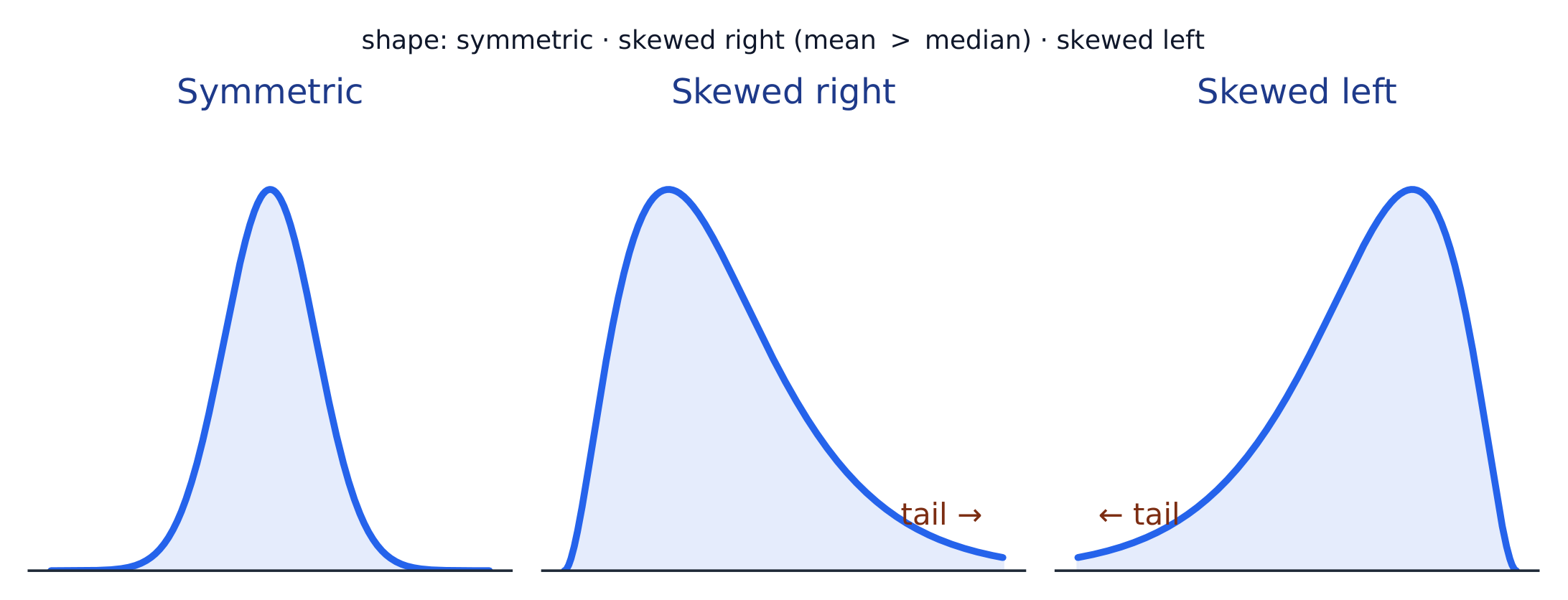
    รูปร่างของการแจกแจง: สมมาตร, บิดเบี้ยวไปทางขวา (หางยาวทางขวา), หรือบิดเบี้ยวไปทางซ้าย
    รูปร่างของการแจกแจง: สมมาตร, บิดเบี้ยวไปทางขวา (หางยาวทางขวา), หรือบิดเบี้ยวไปทางซ้าย
    Vocabulary · ⁨คำศัพท์⁩ Train · ⁨ฝึกฝน⁩
    English ไทย
    Shape/ʃeɪp/ รูปร่าง (Shape)
    skewed/skjuːd/ เบี่ยงขวา/ซ้าย
    unimodal/ˌʌnɪˈmɒdl/ แบบโมเดลเดียว
    bimodal/baɪˈmɒdl/ แบบสองยอด
    uniform/ˈjuːnɪfɔːm/ สม่ำเสมอ
    Outliers/ˈaʊtlaɪəz/ ค่าผิดปกติ
    mean/miːn/ ค่าเฉลี่ย
    median/ˈmiːdiːən/ มัธยฐาน
    interquartile range/ˌɪntəˈkwɔːtaɪl reɪndʒ/ ช่วงระหว่างควอไทล์
    1.7

    Summary Statistics for a Quantitative Variable · ⁨สรุปสถิติสำหรับตัวแปรเชิงปริมาณ⁩

    Syllabus · ⁨หลักสูตร⁩
    English
    Enduring UnderstandingLearning ObjectiveEssential Knowledge

    UNC-1
    Graphical representations and statistics allow us to identify and represent key features of data.

    UNC-1.I
    Calculate measures of center and position for quantitative data. [Skill 2.C]

    • UNC-1.I.1 A statistic is a numerical summary of sample data.
    • UNC-1.I.2 The mean is the sum of all the data values divided by the number of values. For a sample, the mean is denoted by $x$-bar: $\bar{x} = \dfrac{1}{n}\sum_{i=1}^{n} x_i$, where $x_i$ represents the $i^{\text{th}}$ data point in the sample and $n$ represents the number of data values in the sample.
    • UNC-1.I.3 The median of a data set is the middle value when data are ordered. When the number of data points is even, the median can take on any value between the two middle values. In AP Statistics, the most commonly used value for the median of a data set with an even number of values is the average of the two middle values.
    • UNC-1.I.4 The first quartile, Q1, is the median of the half of the ordered data set from the minimum to the position of the median. The third quartile, Q3, is the median of the half of the ordered data set from the position of the median to the maximum. Q1 and Q3 form the boundaries for the middle 50% of values in an ordered data set.
    • UNC-1.I.5 The $p^{\text{th}}$ percentile is interpreted as the value that has $p\%$ of the data less than or equal to it.

    UNC-1.J
    Calculate measures of variability for quantitative data. [Skill 2.C]

    • UNC-1.J.1 Three commonly used measures of variability (or spread) in a distribution are the range, interquartile range, and standard deviation.
    • UNC-1.J.2 The range is defined as the difference between the maximum data value and the minimum data value. The interquartile range (IQR) is defined as the difference between the third and first quartiles: $Q3 - Q1$. Both the range and the interquartile range are possible ways of measuring variability of the distribution of a quantitative variable.
    • UNC-1.J.3 Standard deviation is a way to measure variability of the distribution of a quantitative variable. For a sample, the standard deviation is denoted by $s$: $s_x = \sqrt{\dfrac{1}{n-1}\sum(x_i - \bar{x})^2}$. The square of the sample standard deviation, $s^2$, is called the sample variance.
    • UNC-1.J.4 Changing units of measurement affects the values of the calculated statistics.

    UNC-1.K
    Explain the selection of a particular measure of center and/or variability for describing a set of quantitative data. [Skill 4.B]

    • UNC-1.K.1 There are many methods for determining outliers. Two methods frequently used in this course are:
      • UNC-1.K.1.i An outlier is a value greater than $1.5 \times \text{IQR}$ above the third quartile or more than $1.5 \times \text{IQR}$ below the first quartile.
      • UNC-1.K.1.ii An outlier is a value located 2 or more standard deviations above, or below, the mean.
    • UNC-1.K.2 The mean, standard deviation, and range are considered nonresistant (or non-robust) because they are influenced by outliers. The median and IQR are considered resistant (or robust), because outliers do not greatly (if at all) affect their value.
    ไทย

    ความเข้าใจที่ยั่งยืน (UNC-1): กราฟและสถิติช่วยให้เราระบุและแสดงคุณลักษณะสำคัญของข้อมูลได้ วัตถุประสงค์การเรียนรู้ UNC-1.I: คำนวณขนาดวัดจุดศูนย์กลางและตำแหน่งสำหรับข้อมูลเชิงปริมาณ [ทักษะ 2.C]

    • UNC-1.I.1 สถิติคือสรุปผลตัวเลขของข้อมูลตัวอย่าง
    • UNC-1.I.2 ค่าเฉลี่ย (mean) คือผลรวมของข้อมูลทั้งหมดหารด้วยจำนวนข้อมูล สำหรับตัวอย่าง ค่าเฉลี่ยแสดงด้วย $x$-บาร์: $\bar{x} = \dfrac{1}{n}\sum_{i=1}^{n} x_i$ โดยที่ $x_i$ แทน $i^{\text{th}}$ จุดข้อมูลในตัวอย่าง และ $n$ แทนจำนวนค่าข้อมูลในตัวอย่าง
    • UNC-1.I.3 ค่ามัธยฐาน (median) ของชุดข้อมูลคือค่าที่อยู่ตรงกลางเมื่อเรียงลำดับข้อมูล เมื่อจำนวนจุดข้อมูลเป็นเลขคู่ ค่ามัธยฐานอาจมีค่าใดก็ได้ระหว่างสองค่าตรงกลาง ใน AP Statistics ค่าที่ใช้บ่อยที่สุดสำหรับค่ามัธยฐานของชุดข้อมูลที่มีจำนวนค่าเป็นเลขคู่คือค่าเฉลี่ยของสองค่าตรงกลาง
    • UNC-1.I.4 ควอไทล์แรก, Q1, คือค่ามัธยฐานของครึ่งหนึ่งของชุดข้อมูลที่เรียงลำดับตั้งแต่ค่าต่ำสุดไปจนถึงตำแหน่งของค่ามัธยฐาน ควอไทล์ที่สาม, Q3, คือค่ามัธยฐานของครึ่งหนึ่งของชุดข้อมูลที่เรียงลำดับจากตำแหน่งของค่ามัธยฐานไปถึงค่าสูงสุด Q1 และ Q3 เป็นขอบเขตสำหรับ 50% ของค่าตรงกลางในชุดข้อมูลที่เรียงลำดับ
    • UNC-1.I.5 $p^{\text{th}}$ เปอร์เซ็นต์ไทล์ interpreted ว่ามีค่าซึ่งมี $p\%$ ของข้อมูลน้อยกว่าหรือเท่ากับค่านั้น
    Learning ObjectiveEssential Knowledge

    UNC-1.J
    คำนวณ Measures of variability สำหรับข้อมูลเชิงปริมาณ [Skill 2.C]

    • UNC-1.J.1 Three measures of variability (or spread) ที่ใช้กันทั่วไปในการกระจายคือ range, interquartile range และ standard deviation
    • UNC-1.J.2 Range นิยามว่าเป็นผลต่างระหว่างค่าข้อมูลสูงสุดและค่าข้อมูลต่ำสุด Interquartile range (IQR) นิยามว่าเป็นผลต่างระหว่างควอไทล์ที่สามและควอไทล์แรก: $Q3 - Q1$ ทั้ง range และ interquartile range เป็นวิธีการที่เป็นไปได้ในการวัดความแปรปรวนของการกระจายของตัวแปรเชิงปริมาณ
    • UNC-1.J.3 Standard deviation เป็นวิธีวัดความแปรปรวนของการกระจายของตัวแปรเชิงปริมาณ สำหรับตัวอย่าง standard deviation แสดงด้วย $s$: $s_x = \sqrt{\dfrac{1}{n-1}\sum(x_i - \bar{x})^2}$ สี่เหลี่ยมของ sample standard deviation, $s^2$, เรียกว่า sample variance
    • UNC-1.J.4 การเปลี่ยนหน่วยวัดมีผลต่อค่าของสถิติที่คำนวณได้

    UNC-1.K
    อธิบายการเลือก Measure of center และ/หรือ measure of variability เพื่ออธิบายชุดข้อมูลเชิงปริมาณ [Skill 4.B]

    • UNC-1.K.1 มีหลายวิธีในการระบุค่าผิดปกติ (outliers) Two methods ที่ใช้บ่อยในรายวิชานี้คือ:
      • UNC-1.K.1.i Outlier คือค่ามากกว่า $1.5 \times \text{IQR}$ เหนือควอไทล์ที่สามหรือน้อยกว่า $1.5 \times \text{IQR}$ ต่ำกว่าควอไทล์แรก
      • UNC-1.K.1.ii Outlier คือค่าที่อยู่ห่าง 2 หรือมากกว่า standard deviation เหนือหรือต่ำกว่า mean
    • UNC-1.K.2 Mean, standard deviation และ range被视为 nonresistant (หรือ non-robust) เพราะได้รับผลกระทบจาก outliers Median และ IQR被视为 resistant (หรือ robust), เพราะ outliers ไม่ส่งผลกระทบต่อค่าของพวกมันอย่างมีนัยสำคัญ (ถ้ามีเลย)

    Source: College Board AP Course and Exam Description · ⁨แหล่งที่มา: คำอธิบายหลักสูตรและข้อสอบ College Board AP⁩

    English
    Standard deviation: spread about the mean
    • Center: the mean 均值 $\bar{x}=\dfrac{\sum x_i}{n}$ (average) and the median 中位数 (middle value). The median resists outliers; the mean is pulled toward a skew.
    • Spread: the range, the interquartile range 四分位距 $\text{IQR}=Q_3-Q_1$ (middle 50%), and the standard deviation 标准差 $s_x=\sqrt{\dfrac{\sum(x_i-\bar{x})^2}{n-1}}$ (typical distance from the mean; its square is the variance 方差).
    • The five-number summary 五数概括: min, $Q_1$, median, $Q_3$, max.

    Use resistant measures (median, IQR) for skewed data; mean and standard deviation for roughly symmetric data.

    The percentile 百分位数 of a value is the percent of the data at or below it – so the median is the 50th percentile and $Q_1$ the 25th. A cumulative relative frequency graph 累积相对频率图 makes percentiles easy to read: for each value it plots the proportion of the data at or below it, rising from 0 to 1. Go up from a value to the curve and across to its percentile, or reverse the steps to find the value at a given percentile (the same reading works from a cumulative-frequency table).

    Worked example. For the data $4, 8, 6, 10, 7$: the mean is $\bar{x}=\dfrac{4+8+6+10+7}{5}=\dfrac{35}{5}=7$. Sorting to $4,6,7,8,10$, the median is the middle value, $7$. The mean and median agree here because the data are roughly symmetric.

    ไทย
    ส่วนเบี่ยงเบนมาตรฐาน: การกระจายรอบค่าเฉลี่ย
    • จุดกึ่งกลาง: ค่า เฉลี่ย $\bar{x}=\dfrac{\sum x_i}{n}$ (ค่าเฉลี่ย) และ ค่ามัธยฐาน (ค่าตรงกลาง) ค่ามัธยฐานทนต่อค่าผิดปกติ; แต่ค่าเฉลี่ยจะถูกดึงไปทางความเบ้.
    • การกระจายตัว: ช่วง, ช่วงระหว่างควอไทล์ $\text{IQR}=Q_3-Q_1$ (50% ตรงกลาง), และ ส่วนเบี่ยงเบนมาตรฐาน $s_x=\sqrt{\dfrac{\sum(x_i-\bar{x})^2}{n-1}}$ (ระยะห่างจากค่าเฉลี่ยโดยทั่วไป;กำลังสองของมันคือ ความแปรปรวน).
    • สรุปข้อมูลห้าจำนวน: ค่าน้อยสุด, $Q_1$, ค่ามัธยฐาน, $Q_3$, ค่ามากสุด.

    ใช้ ค่าที่ทนทาน (ค่ามัธยฐาน, IQR) สำหรับข้อมูลที่มีเบ้; ใช้ค่าเฉลี่ยและส่วนเบี่ยงเบนมาตรฐานสำหรับข้อมูลที่ประมาณได้ว่าเป็นสมมาตร.

    เปอร์เซ็นต์ิล ของค่าหนึ่ง คือเปอร์เซ็นต์ของข้อมูลที่น้อยกว่าหรือเท่ากับค่านั้น – ดังนั้นค่ามัธยฐานจึงเป็นเปอร์เซ็นต์ิลที่ 50 และ $Q_1$ เป็นเปอร์เซ็นต์ิลที่ 25. กราฟความถี่สะสมสัมพัทธ์ ทำให้การอ่านค่าเปอร์เซ็นต์ิลได้ง่าย: สำหรับแต่ละค่าจะพล็อตสัดส่วนของข้อมูล ที่น้อยกว่าหรือเท่ากับ ค่านั้น ซึ่งเพิ่มขึ้นจาก 0 ถึง 1. ลากเส้นขึ้นจากค่าไปยังกราฟ แล้วลากข้ามไปหาเปอร์เซ็นต์ิล, หรือทำขั้นตอนย้อนกลับเพื่อหาค่าที่เปอร์เซ็นต์ิลที่กำหนด (การอ่านแบบเดียวกันใช้ได้กับตารางความถี่สะสมด้วย).

    ตัวอย่างวิธีทำ. สำหรับข้อมูล $4, 8, 6, 10, 7$: ค่าเฉลี่ยคือ $\bar{x}=\dfrac{4+8+6+10+7}{5}=\dfrac{35}{5}=7$. เมื่อเรียงลำดับเป็น $4,6,7,8,10$,Median คือค่าตรงกลาง, $7$. ค่าเฉลี่ยและ Median ตรงกันในที่นี้เพราะข้อมูลมีความสมมาตรโดยประมาณ

    Vocabulary · ⁨คำศัพท์⁩ Train · ⁨ฝึกฝน⁩
    English ไทย
    standard deviation/ˈstændəd ˌdiːvɪˈeɪʃn/ ส่วนเบี่ยงเบนมาตรฐาน
    variance/ˈveərɪəns/ ความแปรปรวน
    five-number summary/faɪv ˈnʌmbə ˈsʌməri/ five-number summary
    percentile/pəˈsentaɪl/ เปอร์ไทล์
    cumulative relative frequency graph/ˈkjuːmjʊlətɪv ˈrelətɪv ˈfriːkwənsi ɡræf/ กราฟความถี่สะสมสัมพัทธ์
    1.8

    Graphical Representations of Summary Statistics · ⁨การแสดงภาพสรุปสถิติ⁩

    Syllabus · ⁨หลักสูตร⁩
    English
    Enduring UnderstandingLearning ObjectiveEssential Knowledge

    UNC-1
    Graphical representations and statistics allow us to identify and represent key features of data.

    UNC-1.L
    Represent summary statistics for quantitative data graphically. [Skill 2.B]

    • UNC-1.L.1 Taken together, the minimum data value, the first quartile (Q1), the median, the third quartile (Q3), and the maximum data value make up the five-number summary.
    • UNC-1.L.2 A boxplot is a graphical representation of the five-number summary (minimum, first quartile, median, third quartile, maximum). The box represents the middle 50% of data, with a line at the median and the ends of the box corresponding to the quartiles. Lines ("whiskers") extend from the quartiles to the most extreme point that is not an outlier, and outliers are indicated by their own symbol beyond this.

    UNC-1.M
    Describe summary statistics of quantitative data represented graphically. [Skill 2.A]

    • UNC-1.M.1 Summary statistics of quantitative data, or of sets of quantitative data, can be used to justify claims about the data in context.
    • UNC-1.M.2 If a distribution is relatively symmetric, then the mean and median are relatively close to one another. If a distribution is skewed right, then the mean is usually to the right of the median. If the distribution is skewed left, then the mean is usually to the left of the median.
    ไทย

    ความเข้าใจที่ยั่งยืน (UNC-1): กราฟและสถิติช่วยให้เราระบุและแสดงคุณลักษณะสำคัญของข้อมูลได้

    Learning ObjectiveEssential Knowledge

    UNC-1.L
    แสดง Summary statistics ของข้อมูลเชิงปริมาณแบบกราฟิก [Skill 2.B]

    • UNC-1.L.1 รวมกันแล้ว ค่าข้อมูลต่ำสุด, ควอไทล์แรก (Q1), ค่ามัธยฐาน, ควอไทล์ที่สาม (Q3), และค่าข้อมูลสูงสุด构成了 Five-number summary
    • UNC-1.L.2 Boxplot คือการแสดง Summary statistics แบบกราฟิกของ five-number summary (minimum, first quartile, median, third quartile, maximum) กล่องแทน 50% ตรงกลางของข้อมูล โดยมีเส้นที่ค่ามัธยฐานและปลายกล่องสอดคล้องกับควอไทล์ เส้น ("whiskers") ขยายจากควอไทล์ไปยังจุดที่รุนแรงที่สุดที่ไม่ใช่ outlier และ outliers จะถูกแสดงด้วยสัญลักษณ์ของตนเองเกินกว่านี้

    UNC-1.M
    อธิบาย Summary statistics ของข้อมูลเชิงปริมาณที่แสดงแบบกราฟิก [Skill 2.A]

    • UNC-1.M.1 Summary statistics ของข้อมูลเชิงปริมาณ, หรือของชุดข้อมูลเชิงปริมาณ, สามารถใช้เพื่อสนับสนุนข้ออ้างเกี่ยวกับข้อมูลในบริบทได้
    • UNC-1.M.2 หากการกระจายมีความสมมาตรอย่าง نسبی, แล้ว mean และ median จะอยู่ใกล้กันอย่าง نسبی หากการกระจายเบี่ยงไปทางขวา, แล้ว mean มักจะอยู่ทางขวาของค่ามัธยฐาน หากการกระจายเบี่ยงไปทางซ้าย, แล้ว mean มักจะอยู่ทางซ้ายของค่ามัธยฐาน

    Source: College Board AP Course and Exam Description · ⁨แหล่งที่มา: คำอธิบายหลักสูตรและข้อสอบ College Board AP⁩

    English

    A boxplot 箱线图 draws the five-number summary: a box from $Q_1$ to $Q_3$ with the median inside, and whiskers to the most extreme non-outlier values. A point is an outlier if it lies more than $1.5\times\text{IQR}$ beyond a quartile – a rule you may be asked to apply. Boxplots are ideal for comparing several groups side by side.

    Worked example. A dataset has $Q_1=20$ and $Q_3=32$, so $\text{IQR}=12$. The outlier fences are $Q_1-1.5(12)=2$ and $Q_3+1.5(12)=50$. Any value below $2$ or above $50$ is flagged as an outlier.

    ไทย

    แผนภาพกล่อง แสดงสรุปข้อมูลห้าจำนวน: กล่องจาก $Q_1$ ถึง $Q_3$ โดยมีค่ามัธยฐานอยู่ภายใน, และหนวดไปยังค่าที่รุนแรงที่สุดที่ไม่ใช่ค่าผิดปกติ. จุดหนึ่งถือเป็น ค่าผิดปกติ หากอยู่ไกลกว่า $1.5\times\text{IQR}$ จากควอไทล์ – ซึ่งเป็นกฎที่คุณอาจถูกขอให้นำไปใช้. แผนภาพกล่องเหมาะสำหรับการเปรียบเทียบหลายกลุ่มข้างเคียง.

    **ตัวอย่างคำนวณ.**的一组ข้อมูลมี $Q_1=20$ และ $Q_3=32$, ดังนั้น $\text{IQR}=12$. ขอบเขตค่าผิดปกติคือ $Q_1-1.5(12)=2$ และ $Q_3+1.5(12)=50$. ค่าใดต่ำกว่า $2$ หรือสูงกว่า $50$ จะถูก标记เป็นค่าผิดปกติ.

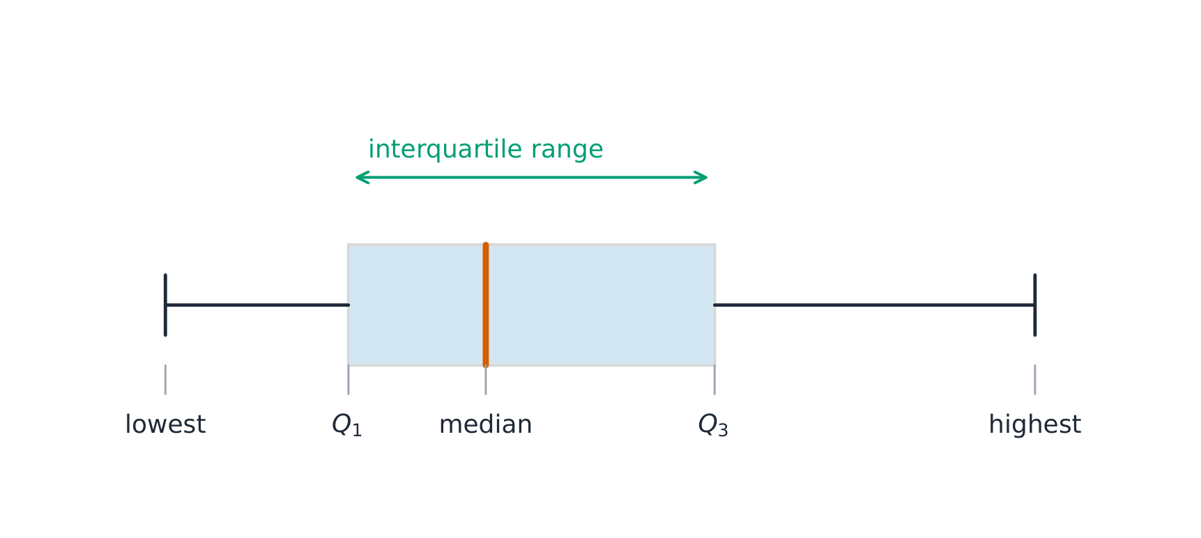
    แผนภาพกล่องและหนวดแสดงควอไทล์และช่วง
    แผนภาพกล่องและหนวดแสดงควอไทล์และช่วง
    แผนภาพกล่องแสดงสรุปข้อมูลห้าจำนวน; กล่องครอบคลุมช่วงระหว่างควอไทล์
    แผนภาพกล่องแสดงสรุปข้อมูลห้าจำนวน; กล่องครอบคลุมช่วงระหว่างควอไทล์
    Explore · ⁨สำรวจ⁩

    Explore the five-number summary as a boxplot · ⁨สำรวจสรุปห้าจำนวนในฐานะกราฟกล่อง⁩

    Drag $Q_1$, the median, and $Q_3$ to see the box (its length is the IQR) and how the median's position inside the box reveals skew — a median close to $Q_1$ signals a right-skewed distribution. · ⁨ลาก $Q_1$, ค่ามัธยฐาน, และ $Q_3$ เพื่อดูกล่อง (ความยาวคือ IQR) และตำแหน่งของค่ามัธยฐานภายในกล่องเผยให้เห็น ความเบ้ — ค่ามัธยฐานใกล้กับ $Q_1$ บ่งชี้ถึงการกระจายตัวแบบเบ้ขวา⁩

    Vocabulary · ⁨คำศัพท์⁩ Train · ⁨ฝึกฝน⁩
    English ไทย
    boxplot/ˈbɒksplɒt/ boxplot
    normal distribution/ˈnɔːml ˌdɪstrɪˈbjuːʃn/ การแจกแจงปกติ
    1.9

    Comparing Distributions of a Quantitative Variable · ⁨เปรียบเทียบการแจกแจงของตัวแปรเชิงปริมาณ⁩

    Syllabus · ⁨หลักสูตร⁩
    English
    Enduring UnderstandingLearning ObjectiveEssential Knowledge

    UNC-1
    Graphical representations and statistics allow us to identify and represent key features of data.

    UNC-1.N
    Compare graphical representations for multiple sets of quantitative data. [Skill 2.D]

    • UNC-1.N.1 Any of the graphical representations, e.g., histograms, side-by-side boxplots, etc., can be used to compare two or more independent samples on center, variability, clusters, gaps, outliers, and other features.

    UNC-1.O
    Compare summary statistics for multiple sets of quantitative data. [Skill 2.D]

    • UNC-1.O.1 Any of the numerical summaries (e.g., mean, standard deviation, relative frequency, etc.) can be used to compare two or more independent samples.
    ไทย

    ความเข้าใจที่ยั่งยืน (UNC-1): กราฟและสถิติช่วยให้เราระบุและแสดงคุณลักษณะสำคัญของข้อมูลได้

    Learning ObjectiveEssential Knowledge

    UNC-1.N
    เปรียบเทียบการแสดงแบบกราฟิกสำหรับหลายชุดข้อมูลเชิงปริมาณ [Skill 2.D]

    • UNC-1.N.1 Any graphical representations, e.g., histograms, side-by-side boxplots, etc., สามารถใช้ในการเปรียบเทียบสองหรือมากกว่า samples独立กัน regarding center, variability, clusters, gaps, outliers, และลักษณะอื่นๆ

    UNC-1.O
    เปรียบเทียบ Summary statistics สำหรับหลายชุดข้อมูลเชิงปริมาณ [Skill 2.D]

    • UNC-1.O.1 Any numerical summaries (e.g., mean, standard deviation, relative frequency, etc.) สามารถใช้ในการเปรียบเทียบสองหรือมากกว่า samples独立กัน

    Source: College Board AP Course and Exam Description · ⁨แหล่งที่มา: คำอธิบายหลักสูตรและข้อสอบ College Board AP⁩

    English

    To compare two or more groups, compare shape, center, and spread, and mention outliers – always with comparative words ("Group A has a higher median than Group B") and in context. Do not just describe each group separately; make the comparison explicit.

    ไทย

    ในการเปรียบเทียบสองกลุ่มขึ้นไป ให้เปรียบเทียบ รูปร่าง, จุดกึ่งกลาง, และการกระจายตัว, และกล่าวถึงค่าผิดปกติ – ด้วยคำเปรียบเทียบเสมอ (“กลุ่ม A มีค่ามัธยฐาน สูงกว่า กลุ่ม B”) และในบริบท. อย่าแค่อธิบายแต่ละกลุ่มแยกกัน; ให้มีการเปรียบเทียบอย่างชัดเจน.

    Explore · ⁨สำรวจ⁩

    Compare distributions with box plots · ⁨เปรียบเทียบการกระจายด้วยกราฟกล่อง⁩

    A box plot draws the five-number summary. Placing two box plots on the same scale compares their centre (median), spread (IQR = box width) and skew at a glance — the fair way to compare groups. · ⁨กราฟกล่อง วาดสรุปห้าจำนวน การวางกราฟกล่องสองอันบนสเกลเดียวกันเปรียบเทียบ จุดกึ่งกลาง (ค่ามัธยฐาน), การกระจาย (IQR = ความกว้างของกล่อง) และ ความเบ้ ได้ทันที — วิธีที่ยุติธรรมในการเปรียบเทียบกลุ่ม⁩

    1.10

    The Normal Distribution · ⁨การแจกแจงปกติ⁩

    Syllabus · ⁨หลักสูตร⁩
    English

    Enduring Understanding (VAR-2): The normal distribution can be used to represent some population distributions.

    Learning Objective VAR-2.A: Compare a data distribution to the normal distribution model. [Skill 2.D]

    • VAR-2.A.1 A parameter is a numerical summary of a population.
    • VAR-2.A.2 Some sets of data may be described as approximately normally distributed. A normal curve is mound-shaped and symmetric. The parameters of a normal distribution are the population mean, $\mu$, and the population standard deviation, $\sigma$.
    • VAR-2.A.3 For a normal distribution, approximately 68% of the observations are within 1 standard deviation of the mean, approximately 95% of observations are within 2 standard deviations of the mean, and approximately 99.7% of observations are within 3 standard deviations of the mean. This is called the empirical rule.
    • VAR-2.A.4 Many variables can be modeled by a normal distribution.
      • Illustrative examples for VAR-2.A:
        • Variables that can be modeled by a normal distribution:
          • Body temperature
          • Weight of a loaf of bread

    Learning Objective VAR-2.B: Determine proportions and percentiles from a normal distribution. [Skill 3.A]

    • VAR-2.B.1 A standardized score for a particular data value is calculated as (data value − mean)/(standard deviation), and measures the number of standard deviations a data value falls above or below the mean.
    • VAR-2.B.2 One example of a standardized score is a $z$-score, which is calculated as $z\text{-score} = \left(\dfrac{x_i - \mu}{\sigma}\right)$. A $z$-score measures how many standard deviations a data value is from the mean.
    • VAR-2.B.3 Technology, such as a calculator, a standard normal table, or computer-generated output, can be used to find the proportion of data values located on a given interval of a normally distributed random variable.
    • VAR-2.B.4 Given the area of a region under the graph of the normal distribution curve, it is possible to use technology, such as a calculator, a standard normal table, or computer-generated output, to estimate parameters for some populations.

    Learning Objective VAR-2.C: Compare measures of relative position in data sets. [Skill 2.D]

    • VAR-2.C.1 Percentiles and $z$-scores may be used to compare relative positions of points within a data set or between data sets.
    ไทย

    ความเข้าใจที่ยั่งยืน (VAR-2): การแจกแจงปกติสามารถใช้เพื่อแสดงการแจกแจงของประชากรบางประเภท

    จุดประสงค์การเรียนรู้ VAR-2.A: เปรียบเทียบการแจกแจงข้อมูลกับโมเดลการแจกแจงปกติ [ทักษะ 2.D]

    • VAR-2.A.1 พารามิเตอร์คือสรุปรายละเอียดเชิงตัวเลขของประชากร
    • VAR-2.A.2 ชุดข้อมูลบางชุดอาจถูกอธิบายว่าเป็นการแจกแจงแบบปกติโดยประมาณ กราฟ normal curve มีรูปร่างคล้ายยอดเขาและสมมาตร พารามิเตอร์ของการแจกแจงปกติคือค่าเฉลี่ยของประชากร, $\mu$, และความเบี่ยงเบนมาตรฐานของประชากร, $\sigma$.
    • VAR-2.A.3 สำหรับการแจกแจงปกติ ประมาณ 68% ของการสังเกตจะอยู่ภายใน 1 ความเบี่ยงเบนมาตรฐานจากค่าเฉลี่ย ประมาณ 95% ของการสังเกตจะอยู่ภายใน 2 ความเบี่ยงเบนมาตรฐานจากค่าเฉลี่ย และประมาณ 99.7% ของการสังเกตจะอยู่ภายใน 3 ความเบี่ยงเบนมาตรฐานจากค่าเฉลี่ย สิ่งนี้เรียกว่ากฎเชิงประจักษ์
    • VAR-2.A.4 ตัวแปรจำนวนมากสามารถจำลองได้ด้วยการแจกแจงปกติ
      • ตัวอย่างประกอบสำหรับ VAR-2.A:
        • ตัวแปรที่สามารถจำลองได้ด้วยการแจกแจงปกติ:
          • อุณหภูมิร่างกาย
          • น้ำหนักของขนมปัง

    จุดประสงค์การเรียนรู้ VAR-2.B: คำนวณสัดส่วนและpercentile จาก distribution แบบปกติ [ทักษะ 3.A]

    • VAR-2.B.1 คะแนนมาตรฐานสำหรับค่าข้อมูลเฉพาะคำนวณได้จาก (ค่าข้อมูล − ค่าเฉลี่ย)/(ความเบี่ยงเบนมาตรฐาน) และวัดจำนวนความเบี่ยงเบนมาตรฐานที่ค่าข้อมูลนั้นห่างจากค่าเฉลี่ยไปทางด้านบนหรือด้านล่าง
    • VAR-2.B.2 ตัวอย่างหนึ่งของคะแนนมาตรฐานคือ $z$-score, ซึ่งคำนวณได้จาก $z\text{-score} = \left(\dfrac{x_i - \mu}{\sigma}\right)$. A $z$-score วัดว่าค่าข้อมูลห่างจากค่าเฉลี่ยกี่ความเบี่ยงเบนมาตรฐาน
    • VAR-2.B.3 เทคโนโลยี เช่น เครื่องคิดเลข ตารางnormal standard หรือผลลัพธ์ที่ผลิตโดยคอมพิวเตอร์ สามารถใช้ในการหาสัดส่วนของค่าข้อมูลที่อยู่ภายในช่วงที่กำหนดของตัวแปรสุ่มที่แจกแจงแบบปกติ
    • VAR-2.B.4 เมื่อทราบพื้นที่ของภูมิภาคใต้กราฟ of the normal distribution curve เป็นไปได้ที่จะใช้เทคโนโลยี เช่น เครื่องคิดเลข ตารางnormal standard หรือผลลัพธ์ที่ผลิตโดยคอมพิวเตอร์ เพื่อประมาณค่าพารามิเตอร์สำหรับบางประชากร

    จุดประสงค์การเรียนรู้ VAR-2.C: เปรียบเทียบมาตรการของตำแหน่งสัมพัทธ์ในชุดข้อมูล [ทักษะ 2.D]

    • VAR-2.C.1 Percentiles และ $z$-scores อาจใช้เพื่อเปรียบเทียบตำแหน่งสัมพัทธ์ของจุดภายในชุดข้อมูลหรือระหว่างชุดข้อมูล

    Source: College Board AP Course and Exam Description · ⁨แหล่งที่มา: คำอธิบายหลักสูตรและข้อสอบ College Board AP⁩

    English

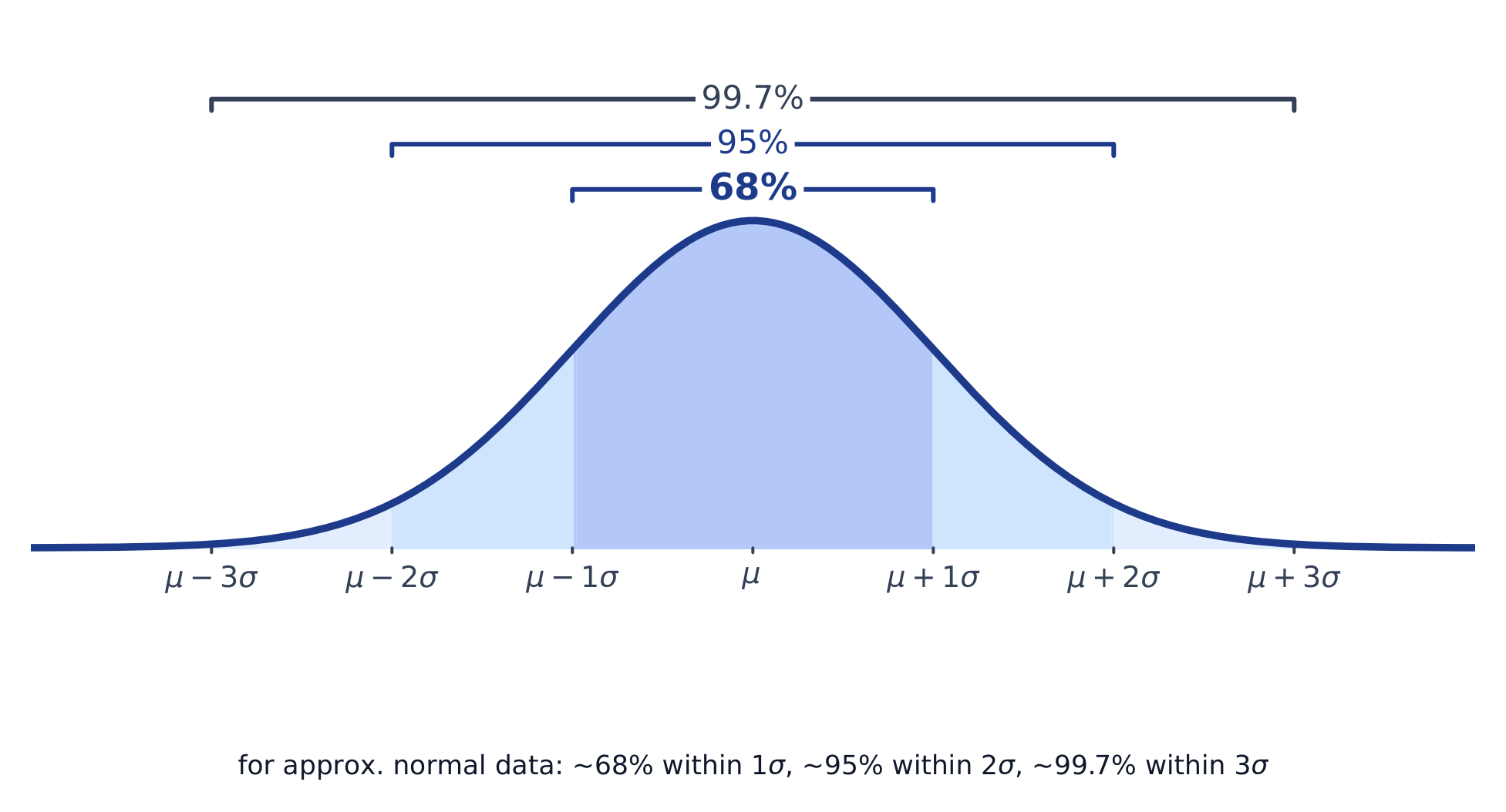
    A normal distribution 正态分布 is a symmetric, bell-shaped model described by its mean $\mu$ and standard deviation $\sigma$. The empirical rule 经验法则 (68–95–99.7): about 68% of values lie within $1\sigma$ of the mean, 95% within $2\sigma$, and 99.7% within $3\sigma$.

    A $z$-score 标准分数 measures how many standard deviations a value is from the mean:

    $$z=\frac{x-\mu}{\sigma}.$$
    Convert to a $z$-score, then use the normal table or technology to find the proportion (area) below, above, or between values – and reverse the process to find a value from a given percentile.

    Worked example. Test scores are normal with $\mu=500$ and $\sigma=100$. A score of $700$ has $z=\dfrac{700-500}{100}=2$. By the empirical rule, $95\%$ of scores lie within $2\sigma$, so $2.5\%$ lie above $700$ – meaning a $700$ is at about the $97.5$th percentile.

    ไทย

    การแจกแจงปกติ เป็นโมเดลสมมาตรรูปกระดิ่งที่อธิบายด้วยค่าเฉลี่ย $\mu$ และส่วนเบี่ยงเบนมาตรฐาน $\sigma$. กฎทฤษฎีบทจริง (68–95–99.7): ประมาณ 68% ของค่าอยู่ในระยะ $1\sigma$ จากค่าเฉลี่ย, 95% Within $2\sigma$, และ 99.7% Within $3\sigma$.

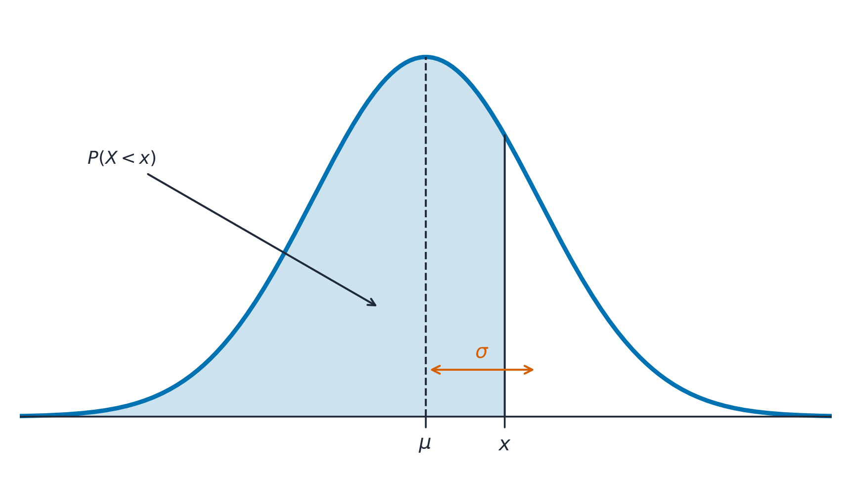
    โค้งปกติ: ความน่าจะเป็นคือพื้นที่ใต้โค้ง ซึ่งศูนย์กลางอยู่ที่ค่าเฉลี่ย
    โค้งปกติ: ความน่าจะเป็นคือพื้นที่ใต้โค้ง ซึ่งศูนย์กลางอยู่ที่ค่าเฉลี่ย

    ค่า $z$-score วัดว่าค่าหนึ่งห่างจากค่าเฉลี่ยกี่ส่วนเบี่ยงเบนมาตรฐาน:

    $$z=\frac{x-\mu}{\sigma}.$$
    แปลงเป็น $z$-score, จากนั้นใช้ตารางการแจกแจงปกติหรือเทคโนโลยีเพื่อหา สัดส่วน (พื้นที่) ด้านล่าง, ด้านบน, หรือระหว่างค่า – และทำขั้นตอนย้อนกลับเพื่อหาค่าจากเปอร์เซ็นต์ิลที่กำหนด.

    ตัวอย่างวิธีทำ. คะแนนทดสอบมีการแจกแจงปกติด้วย $\mu=500$ และ $\sigma=100$. คะแนน $700$ มี $z=\dfrac{700-500}{100}=2$. ตามกฎเชิงประจักษ์, $95\%$ ของคะแนนอยู่ภายใน $2\sigma$, ดังนั้น $2.5\%$ อยู่เหนือ $700$ – ซึ่งหมายความว่า $700$ อยู่ที่เปอร์เซ็นต์ิลที่ประมาณ $97.5$

    เส้นโค้งปกติและกฎทฤษฎีบทจริง 68-95-99.7
    เส้นโค้งปกติและกฎทฤษฎีบทจริง 68-95-99.7
    Explore · ⁨สำรวจ⁩

    Explore area under the normal curve · ⁨สำรวจพื้นที่ใต้เส้นโค้งปกติ⁩

    The proportion of data below a value equals the area under the curve to its left. Shade a tail or a central band to see the 68–95–99.7 empirical rule and read a $z$-score as an area. · ⁨สัดส่วน ของข้อมูลต่ำกว่าค่าหนึ่งเท่ากับ พื้นที่ใต้เส้นโค้งทางซ้ายของมัน ทาเงาส่วนหางหรือแถบตรงกลางเพื่อดูกฎเชิงประจักษ์ 68–95–99.7 และอ่านค่า $z$ เป็นพื้นที่⁩

    Vocabulary · ⁨คำศัพท์⁩ Train · ⁨ฝึกฝน⁩
    English ไทย
    empirical rule/emˈpɪrɪkl ruːl/ กฎเชิงประจักษ์ (empirical rule)
    $z$-score/ˈzed skɔː/ $z$-สโคร์
    1.10

    Exam tips · ⁨ข้อแนะนำสำหรับการสอบ⁩

    English
    • Describe a distribution by shape, center, spread, and outliers (SOCS) — always in context.
    • The mean is pulled by outliers; the median resists them, so prefer the median for skewed data.
    • For a normal distribution use the 68–95–99.7 rule and z-scores $z=\tfrac{x-\mu}{\sigma}$.
    • Compare distributions with side-by-side boxplots and comment on center, spread, and shape.
    • Standard deviation measures a typical distance from the mean; the IQR pairs with the median.
    ไทย
    • อธิบายการแจกแจงด้วย รูปร่าง, จุดกึ่งกลาง, การกระจายตัว, และค่าผิดปกติ (SOCS) – เสมอในบริบท.
    • ค่าเฉลี่ย ถูกดึงโดยค่าผิดปกติ; ค่ามัธยฐาน ทนต่อมันได้ ดังนั้นควรเลือกค่ามัธยฐานสำหรับข้อมูลที่มีเบ้.
    • สำหรับการแจกแจง ปกติ ใช้กฎ 68–95–99.7 และ z-scores $z=\tfrac{x-\mu}{\sigma}$.
    • เปรียบเทียบการแจกแจงด้วยแผนภาพกล่องข้างเคียงและคอมเมนต์เรื่องจุดกึ่งกลาง, การกระจายตัว, และรูปร่าง.
    • ส่วนเบี่ยงเบนมาตรฐานวัดระยะห่างจากค่าเฉลี่ยโดยทั่วไป; IQR คู่กับค่ามัธยฐาน.
  • 2

    Exploring Two-Variable Data · ⁨การสำรวจข้อมูลสองตัวแปร⁩

    Watch lesson · ⁨ดูบทเรียน⁩
    2.1

    Are Two Variables Related? · ⁨ตัวแปรสองตัวมีความสัมพันธ์กันหรือไม่?⁩

    Syllabus · ⁨หลักสูตร⁩
    English
    Enduring UnderstandingLearning ObjectiveEssential Knowledge

    VAR-1
    Given that variation may be random or not, conclusions are uncertain.

    VAR-1.D
    Identify questions to be answered about possible relationships in data. [Skill 1.A]

    • VAR-1.D.1 Apparent patterns and associations in data may be random or not.
    ไทย

    ความเข้าใจที่ยั่งยืน (VAR-1): เนื่องจากความแปรปรวนอาจเป็นแบบสุ่มหรือไม่ ดังนั้นข้อสรุปจึงมีความไม่แน่นอน

    Learning ObjectiveEssential Knowledge

    VAR-1.D
    ระบุคำถามที่จะตอบเกี่ยวกับความสัมพันธ์ที่เป็นไปได้ในข้อมูล [Skill 1.A]

    • VAR-1.D.1 ลวดลายและความสัมพันธ์ที่ปรากฏในข้อมูลอาจเป็นแบบสุ่มหรือไม่ก็ตาม

    Source: College Board AP Course and Exam Description · ⁨แหล่งที่มา: คำอธิบายหลักสูตรและข้อสอบ College Board AP⁩

    English

    Two-variable data let us ask whether two characteristics are associated 关联 – whether knowing one tells you something about the other. An explanatory variable 解释变量 (the "input") may help predict a response variable 响应变量 (the "output"). Association is not the same as causation.

    ไทย

    ข้อมูลสองตัวแปรช่วยให้เราถามได้ว่าลักษณะสองอย่าง มีความสัมพันธ์ หรือไม่ – ว่าการรู้สิ่งหนึ่งบอกอะไรเกี่ยวกับอีกสิ่งหนึ่งได้หรือไม่. ตัวแปรอธิบาย (“อินพุต”) อาจช่วยทำนาย ตัวแปรตอบสนอง (“เอาต์พุต”). ความสัมพันธ์ไม่เท่ากับสาเหตุ.

    2.2

    Two Categorical Variables · ⁨ตัวแปรเชิงหมวดหมู่สองชนิด⁩

    Syllabus · ⁨หลักสูตร⁩
    English
    Enduring UnderstandingLearning ObjectiveEssential Knowledge

    UNC-1
    Graphical representations and statistics allow us to identify and represent key features of data.

    UNC-1.P
    Compare numerical and graphical representations for two categorical variables. [Skill 2.D]

    • UNC-1.P.1 Side-by-side bar graphs, segmented bar graphs, and mosaic plots are examples of bar graphs for one categorical variable, broken down by categories of another categorical variable.
    • UNC-1.P.2 Graphical representations of two categorical variables can be used to compare distributions and/or determine if variables are associated.
    • UNC-1.P.3 A two-way table, also called a contingency table, is used to summarize two categorical variables. The entries in the cells can be frequency counts or relative frequencies.
    • UNC-1.P.4 A joint relative frequency is a cell frequency divided by the total for the entire table.
    ไทย

    ความเข้าใจที่ยั่งยืน (UNC-1): กราฟและสถิติช่วยให้เราระบุและแสดงคุณลักษณะสำคัญของข้อมูลได้

    Learning ObjectiveEssential Knowledge

    UNC-1.P
    เปรียบเทียบการแสดงแบบตัวเลขและกราฟิกสำหรับตัวแปรเชิงหมวดหมู่สองตัว [Skill 2.D]

    • UNC-1.P.1 Side-by-side bar graphs, segmented bar graphs, และ mosaic plots เป็นตัวอย่างของ bar graphs สำหรับตัวแปรเชิงหมวดหมู่หนึ่งตัว ที่แยกย่อยตาม categories ของอีกตัวแปรเชิงหมวดหมู่หนึ่ง
    • UNC-1.P.2 การแสดงแบบกราฟิกของตัวแปรเชิงหมวดหมู่สองตัวสามารถใช้เพื่อเปรียบเทียบการกระจายและ/หรือตรวจสอบว่าตัวแปรสัมพันธ์กันหรือไม่
    • UNC-1.P.3 ตารางสองทาง หรือที่เรียกว่าตารางความถ่วง (contingency table) ใช้สำหรับสรุปตัวแปรเชิงหมวดหมู่สองตัว ค่าในเซลล์สามารถเป็นจำนวนความถี่หรือความถี่สัมพัทธ์ได้
    • UNC-1.P.4 ความถี่สัมพัทธ์ร่วม (joint relative frequency) คือความถี่ของเซลล์หารด้วยผลรวมทั้งหมดของตารางทั้งตาราง

    Source: College Board AP Course and Exam Description · ⁨แหล่งที่มา: คำอธิบายหลักสูตรและข้อสอบ College Board AP⁩

    English

    A two-way table 双向表 (contingency table) counts individuals by two categorical variables at once. A marginal distribution 边缘分布 is a row or column total written as a fraction of the grand total (the totals themselves are just counts). Comparing the inside cells shows whether the variables are related.

    ไทย

    ตารางสองมิติ (ตารางความถ่วง) นับจำนวนบุคคลตามตัวแปรเชิงหมวดหมู่สองชนิดพร้อมกัน. การแจกแจงขอบ คือผลรวมแถวหรือคอลัมน์ที่เขียนเป็นเศษส่วนของผลรวมทั้งหมด (ผลรวมเองเป็นเพียงจำนวนนับ). การเปรียบเทียบเซลล์ด้านในแสดงว่าตัวแปรทั้งสองมีความสัมพันธ์กันหรือไม่.

    2.3

    Comparing Groups with Conditional Distributions · ⁨เปรียบเทียบกลุ่มด้วยการแจกแจงแบบเงื่อนไข⁩

    Syllabus · ⁨หลักสูตร⁩
    English

    Enduring Understanding (UNC-1): Graphical representations and statistics allow us to identify and represent key features of data.

    Learning Objective UNC-1.Q: Calculate statistics for two categorical variables. [Skill 2.C]

    • UNC-1.Q.1 The marginal relative frequencies are the row and column totals in a two-way table divided by the total for the entire table.
    • UNC-1.Q.2 A conditional relative frequency is a relative frequency for a specific part of the contingency table (e.g., cell frequencies in a row divided by the total for that row).

    Learning Objective UNC-1.R: Compare statistics for two categorical variables. [Skill 2.D]

    • UNC-1.R.1 Summary statistics for two categorical variables can be used to compare distributions and/or determine if variables are associated.
    ไทย

    ความเข้าใจที่ยั่งยืน (UNC-1): กราฟและสถิติช่วยให้เราระบุและแสดงคุณลักษณะสำคัญของข้อมูลได้

    วัตถุประสงค์การเรียนรู้ UNC-1.Q: คำนวณสถิติสำหรับตัวแปรเชิงหมวดหมู่สองตัว [ทักษะ 2.C]

    • UNC-1.Q.1 ความถี่สัมพัทธ์ขอบ (marginal relative frequencies) คือผลรวมตามแถวและคอลัมน์ในตารางสองทางหารด้วยผลรวมทั้งหมดของตารางทั้งตาราง
    • UNC-1.Q.2 ความถี่สัมพัทธ์เงื่อนไข (conditional relative frequency) คือความถี่สัมพัทธ์สำหรับส่วนเฉพาะหนึ่งของตารางความถ่วง (เช่น ความถี่ของเซลล์ในแถวหารด้วยผลรวมของแถวนั้น)

    วัตถุประสงค์การเรียนรู้ UNC-1.R: เปรียบเทียบสถิติสำหรับตัวแปรเชิงหมวดหมู่สองตัว [ทักษะ 2.D]

    • UNC-1.R.1 สถิติสรุปสำหรับตัวแปรเชิงหมวดหมู่สองตัวสามารถใช้เพื่อเปรียบเทียบการแจกแจงและ/หรือตรวจสอบว่าตัวแปรมีความสัมพันธ์กันหรือไม่

    Source: College Board AP Course and Exam Description · ⁨แหล่งที่มา: คำอธิบายหลักสูตรและข้อสอบ College Board AP⁩

    English

    A conditional distribution 条件分布 is the distribution of one variable within a fixed category of the other (found by dividing each cell by its row or column total). If the conditional distributions differ across groups, the two variables are associated; if they are the same, there is no association. Segmented bar charts 分段条形图 or mosaic plots display them.

    ไทย

    การแจกแจงแบบเงื่อนไข คือการแจกแจงของตัวแปรหนึ่ง ภายใน หมวดหมู่คงที่ของอีกตัวแปรหนึ่ง (หาได้โดยการหารแต่ละเซลล์ด้วยผลรวมแถวหรือคอลัมน์). หากการแจกแจงแบบเงื่อนไขแตกต่างกันข้ามกลุ่ม ตัวแปรทั้งสองจะ มีความสัมพันธ์; หากเหมือนกัน ไม่มีความสัมพันธ์. แผนภาพแท่งแบ่งส่วน หรือแผนภาพโมเสกแสดงการแจกแจงเหล่านี้.

    2.4

    Scatterplots for Two Quantitative Variables · ⁨แผนภาพกระจายสำหรับตัวแปรเชิงปริมาณสองชนิด⁩

    Syllabus · ⁨หลักสูตร⁩
    English

    Enduring Understanding (UNC-1): Graphical representations and statistics allow us to identify and represent key features of data.

    Learning Objective UNC-1.S: Represent bivariate quantitative data using scatterplots. [Skill 2.B]

    • UNC-1.S.1 A bivariate quantitative data set consists of observations of two different quantitative variables made on individuals in a sample or population.
    • UNC-1.S.2 A scatterplot shows two numeric values for each observation, one corresponding to the value on the $x$-axis and one corresponding to the value on the $y$-axis.
    • UNC-1.S.3 An explanatory variable is a variable whose values are used to explain or predict corresponding values for the response variable.

    Enduring Understanding (DAT-1): Regression models may allow us to predict responses to changes in an explanatory variable.

    Learning Objective DAT-1.A: Describe the characteristics of a scatter plot. [Skill 2.A]

    • DAT-1.A.1 A description of a scatter plot includes form, direction, strength, and unusual features.
    • DAT-1.A.2 The direction of the association shown in a scatterplot, if any, can be described as positive or negative.
    • DAT-1.A.3 A positive association means that as values of one variable increase, the values of the other variable tend to increase. A negative association means that as values of one variable increase, values of the other variable tend to decrease.
    • DAT-1.A.4 The form of the association shown in a scatterplot, if any, can be described as linear or non-linear to varying degrees.
    • DAT-1.A.5 The strength of the association is how closely the individual points follow a specific pattern, e.g., linear, and can be shown in a scatterplot. Strength can be described as strong, moderate, or weak.
    • DAT-1.A.6 Unusual features of a scatter plot include clusters of points or points with relatively large discrepancies between the value of the response variable and a predicted value for the response variable.
    ไทย

    ความเข้าใจที่ยั่งยืน (UNC-1): กราฟและสถิติช่วยให้เราระบุและแสดงคุณลักษณะสำคัญของข้อมูลได้

    วัตถุประสงค์การเรียนรู้ UNC-1.S: แสดงข้อมูลเชิงปริมาณคู่โดยใช้กราฟกระจาย [ทักษะ 2.B]

    • UNC-1.S.1 ชุดข้อมูลเชิงปริมาณคู่ประกอบด้วยข้อสังเกตของตัวแปรเชิงปริมาณสองตัวที่แตกต่างกันซึ่งวัดจากบุคคลในตัวอย่างหรือประชากร
    • UNC-1.S.2 กราฟกระจายแสดงค่าตัวเลขสองค่าสำหรับแต่ละข้อสังเกต โดยค่าหนึ่งสอดคล้องกับค่าบน $x$-แกน และอีกค่าหนึ่งสอดคล้องกับค่าบน $y$-แกน
    • UNC-1.S.3 ตัวแปรอธิบายคือตัวแปรwhose values被用来解释或预测响应变量。

    ความเข้าใจที่ยั่งยืน (DAT-1): แบบจำลองการถดถอยอาจช่วยให้เราทำนายผลลัพธ์จากการเปลี่ยนแปลงในตัวแปรอธิบายได้

    วัตถุประสงค์การเรียนรู้ DAT-1.A: อธิบายลักษณะของกราฟกระจาย [ทักษะ 2.A]

    • DAT-1.A.1 การอธิบายกราฟกระจายประกอบด้วยรูปแบบ ทิศทาง ความเข้ม และลักษณะผิดปกติ
    • DAT-1.A.2 ทิศทางของความสัมพันธ์ที่ปรากฏในกราฟกระจาย หากมี สามารถอธิบายได้ว่าเป็นบวกหรือลบ
    • DAT-1.A.3 ความสัมพันธ์เชิงบวกหมายความว่าเมื่อค่าของตัวแปรหนึ่งเพิ่มขึ้น ค่าของอีกตัวแปรหนึ่งก็มีแนวโน้มที่จะเพิ่มขึ้น ความสัมพันธ์เชิงลบหมายความว่าเมื่อค่าของตัวแปรหนึ่งเพิ่มขึ้น ค่าของอีกตัวแปรหนึ่งมีแนวโน้มที่จะลดลง
    • DAT-1.A.4 รูปแบบของความสัมพันธ์ที่ปรากฏในกราฟกระจาย หากมี สามารถอธิบายได้ว่ามีความเป็นเส้นตรงหรือไม่เป็นเส้นตรงในระดับต่างๆ
    • DAT-1.A.5 ความเข้มของความสัมพันธ์คือระดับที่จุดแต่ละจุดปฏิบัติตามรูปแบบเฉพาะ เช่น เส้นตรง ในกราฟกระจาย ความเข้มสามารถอธิบายได้ว่าแข็งแกร่ง ปานกลาง หรืออ่อน
    • DAT-1.A.6 ลักษณะผิดปกติของกราฟกระจายรวมถึงกลุ่มของจุดหรือจุดที่มีข้อแตกต่างอย่างมีนัยสำคัญระหว่างค่าของตัวแปรตอบสนองกับค่าที่คาดหมายสำหรับตัวแปรตอบสนอง

    Source: College Board AP Course and Exam Description · ⁨แหล่งที่มา: คำอธิบายหลักสูตรและข้อสอบ College Board AP⁩

    English

    A scatterplot 散点图 plots each individual as a point, explanatory variable on the $x$-axis and response on the $y$-axis. Describe it with DUFS: Direction (positive/negative), Unusual features (outliers, clusters), Form (linear or curved), and Strength (how tightly the points follow the pattern) – always in context.

    ไทย

    กราฟกระจาย (scatterplot) แสดงแต่ละบุคคลเป็นจุด โดยตัวแปรอธิบายวางบน $x$ และตัวแปรตอบรับวางบน $y$ อธิบายด้วย DUFS: ทิศทาง (บวก/ลบ), ลักษณะผิดปกติ (ค่าสุดขั้ว, กลุ่ม), รูปแบบ (เชิงเส้นหรือโค้ง), และ ความเข้ม (ความแน่นที่จุดตามรูปแบบ) – ต้องอธิบายในบริบทเสมอ

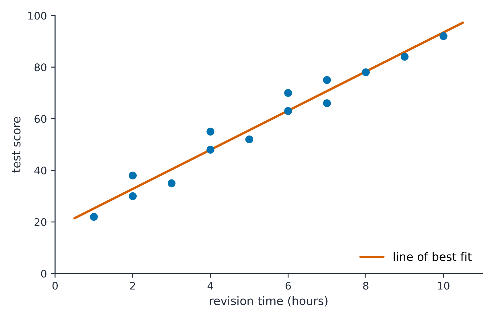
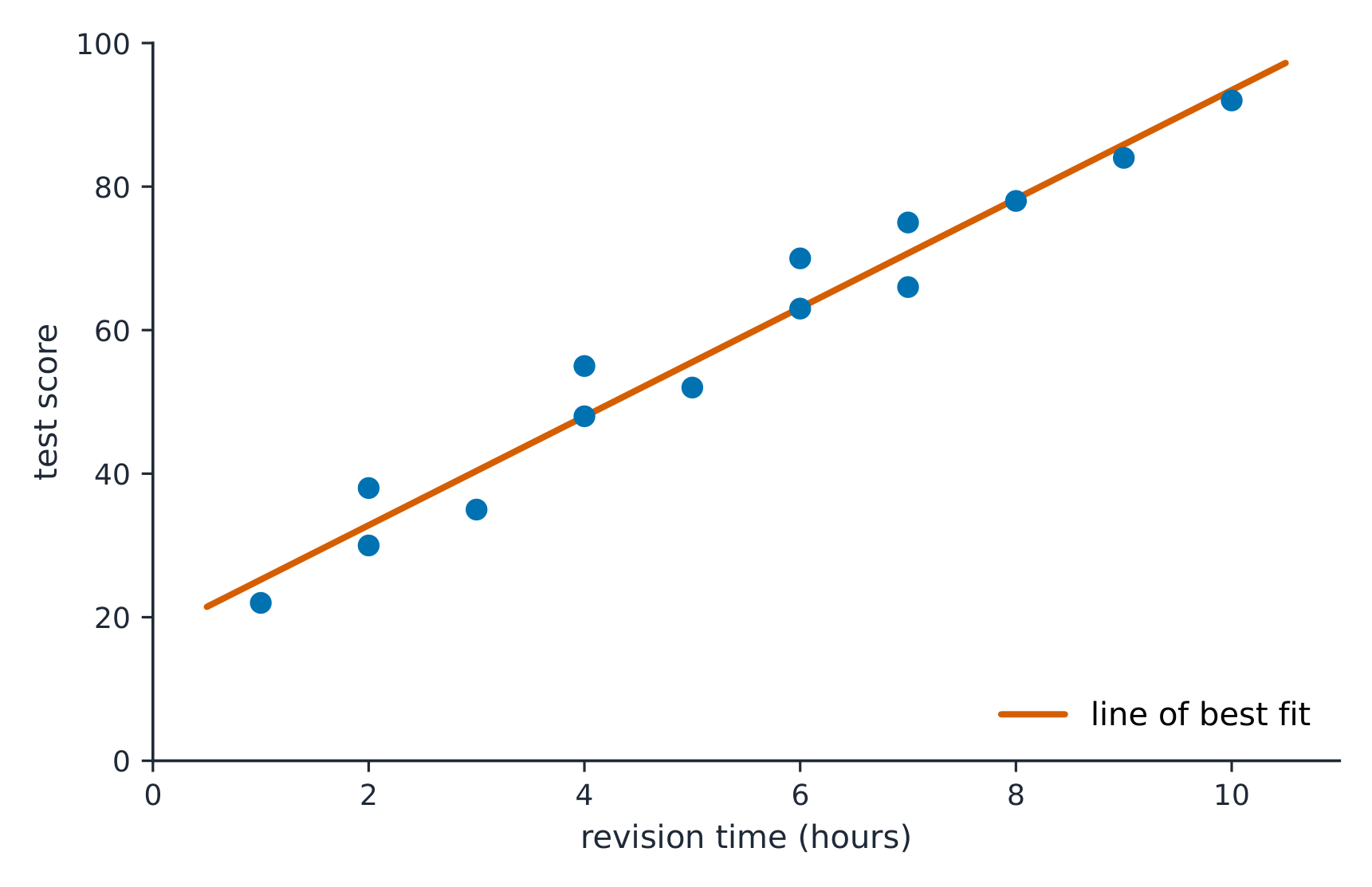
    เส้นประมาณการที่ดีที่สุดวิ่งผ่านกลางกลุ่มจุดกระจาย
    เส้นประมาณการที่ดีที่สุดวิ่งผ่านกลางกลุ่มจุดกระจาย
    Vocabulary · ⁨คำศัพท์⁩ Train · ⁨ฝึกฝน⁩
    English ไทย
    associated/əˈsəʊsɪeɪtɪd/ มีความสัมพันธ์กัน
    explanatory variable/ekˈsplænətəri ˈveərɪəbl/ explanatory variable
    response variable/rɪˈspɒns ˈveərɪəbl/ response variable
    two-way table/tuː weɪ ˈteɪbl/ ตารางสองมิติ
    marginal distributions/ˈmɑːdʒɪnl ˌdɪstrɪˈbjuːʃnz/ การแจกแจงส่วนขอบ
    conditional distribution/kənˈdɪʃənl ˌdɪstrɪˈbjuːʃn/ การแจกแจงแบบมีเงื่อนไข
    Segmented bar charts/seɡˈmentɪd bɑː tʃɑːts/ แผนภูมิแท่งแบบแบ่งส่วน
    scatterplot/ˈskætəplɒt/ แผนภูมิกระจาย (scatterplot)
    2.5

    Correlation · ⁨ความสัมพันธ์⁩

    Syllabus · ⁨หลักสูตร⁩
    English

    Enduring Understanding (DAT-1): Regression models may allow us to predict responses to changes in an explanatory variable.

    Learning Objective DAT-1.B: Determine the correlation for a linear relationship. [Skill 2.C]

    • DAT-1.B.1 The correlation, $r$, gives the direction and quantifies the strength of the linear association between two quantitative variables.
    • DAT-1.B.2 The correlation coefficient can be calculated by: $r = \dfrac{1}{n-1} \sum \left( \dfrac{x_i - \bar{x}}{s_x} \right) \left( \dfrac{y_i - \bar{y}}{s_y} \right)$. However, the most common way to determine $r$ is by using technology.
    • DAT-1.B.3 A correlation coefficient close to 1 or $-1$ does not necessarily mean that a linear model is appropriate.

    Learning Objective DAT-1.C: Interpret the correlation for a linear relationship. [Skill 4.B]

    • DAT-1.C.1 The correlation, $r$, is unit-free, and always between $-1$ and 1, inclusive. A value of $r = 0$ indicates that there is no linear association. A value of $r = 1$ or $r = -1$ indicates that there is a perfect linear association.
    • DAT-1.C.2 A perceived or real relationship between two variables does not mean that changes in one variable cause changes in the other. That is, correlation does not necessarily imply causation.
    ไทย

    ความเข้าใจที่ยั่งยืน (DAT-1): แบบจำลองการถดถอยอาจช่วยให้เราทำนายผลลัพธ์จากการเปลี่ยนแปลงในตัวแปรอธิบายได้

    วัตถุประสงค์การเรียนรู้ DAT-1.B: หาค่าสหประสิทธิผลสำหรับความสัมพันธ์เชิงเส้น [ทักษะ 2.C]

    • DAT-1.B.1 สหประสิทธิผล, $r$, บอกลักษณะทิศทางและวัดระดับความเข้มของความสัมพันธ์เชิงเส้นระหว่างตัวแปรเชิงปริมาณสองตัว
    • DAT-1.B.2 ค่าสัมประสิทธิ์สหสัมพันธ์สามารถคำนวณได้ด้วยสูตร: $r = \dfrac{1}{n-1} \sum \left( \dfrac{x_i - \bar{x}}{s_x} \right) \left( \dfrac{y_i - \bar{y}}{s_y} \right)$ อย่างไรก็ตาม วิธีที่พบบ่อยที่สุดในการหาค่า $r$ คือการใช้เทคโนโลยี
    • DAT-1.B.3 ค่าสัมประสิทธิ์สหประสิทธิผลที่ใกล้กับ 1 หรือ $-1$ ไม่จำเป็นต้องหมายความว่าแบบจำลองเชิงเส้นเหมาะสม

    วัตถุประสงค์การเรียนรู้ DAT-1.C: ตีความค่าสหประสิทธิผลสำหรับความสัมพันธ์เชิงเส้น [ทักษะ 4.B]

    • DAT-1.C.1 สหประสิทธิผล, $r$, เป็นปริมาณไม่มีหน่วย และอยู่ระหว่าง $-1$ ถึง 1 เสมอ ค่าของ $r = 0$ แสดงว่าไม่มีความสัมพันธ์เชิงเส้น ค่าของ $r = 1$ หรือ $r = -1$ แสดงว่ามีความสัมพันธ์เชิงเส้นสมบูรณ์
    • DAT-1.C.2 ความสัมพันธ์ที่รับรู้หรือมีความจริงระหว่างตัวแปรสองตัว并不意味着改变一个变量会导致另一个变量的变化。即,相关性并不必然意味着因果关系。

    Source: College Board AP Course and Exam Description · ⁨แหล่งที่มา: คำอธิบายหลักสูตรและข้อสอบ College Board AP⁩

    English
    What r actually measures

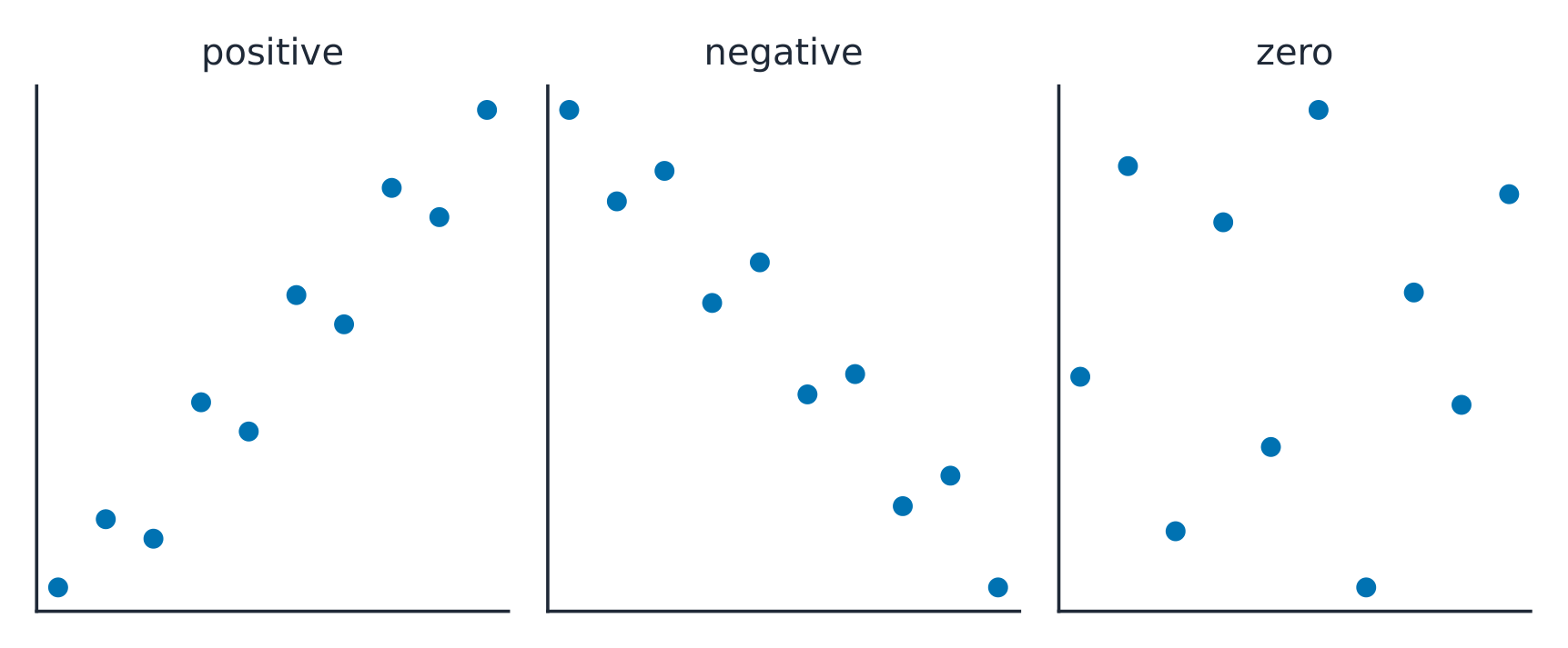
    The correlation coefficient 相关系数 $r$ measures the strength and direction of a linear relationship. It runs from $-1$ to $1$: near $\pm 1$ is strong linear, near $0$ is weak linear. $r$ has no units and does not change if you swap the variables. Warnings: $r$ only measures linear strength, it is not resistant to outliers, and a strong $r$ does not prove causation.

    ไทย
    r วัดอะไรจริงๆ

    สัมประสิทธิ์สหสัมพันธ์ (correlation coefficient) $r$ วัด ความเข้มแข็งและทิศทางของความสัมพันธ์แบบเส้นตรง.它有值从 $-1$ ถึง $1$: Near $\pm 1$ means strong linear relationship, near $0$ means weak linear relationship. $r$ ไม่มีหน่วยและไม่เปลี่ยนเมื่อสลับตัวแปร ข้อควรระวัง: $r$ วัด ความเข้มแข็งแบบเส้นตรง เท่านั้น, ไม่ทนทานต่อค่าผิดปกติ, และค่า $r$ ที่สูง ไม่ได้ บ่งชี้ถึงความสัมพันธ์เชิงเหตุและผล

    สหสัมพันธ์บวกเพิ่มขึ้นพร้อมกัน; สหสัมพันธ์ลบเคลื่อนที่ในทิศทางตรงข้าม
    สหสัมพันธ์บวกเพิ่มขึ้นพร้อมกัน; สหสัมพันธ์ลบเคลื่อนที่ในทิศทางตรงข้าม
    Explore · ⁨สำรวจ⁩

    Strength of a linear relationship · ⁨ความเข้มของความสัมพันธ์เชิงเส้น⁩

    Correlation $r$ runs from $-1$ to $1$: near $\pm1$ the points hug a line, near 0 they scatter. Change it and watch the cloud tighten or spread. · ⁨สหสัมพันธ์ $r$Running จาก $-1$ ถึง $1$: ใกล้กับ $\pm1$ จุดจะเกาะติดเส้น, ใกล้ 0 จะกระจายตัว เปลี่ยนมันและดูเมฆแน่นหรือขยายออก⁩

    Vocabulary · ⁨คำศัพท์⁩ Train · ⁨ฝึกฝน⁩
    English ไทย
    correlation coefficient/ˌkɒrɪˈleɪʃn ˌkəʊɪˈfɪʃənt/ สัมประสิทธิ์สหสัมพันธ์
    2.6

    Linear Regression Models · ⁨โมเดลถดถอยเชิงเส้น⁩

    Syllabus · ⁨หลักสูตร⁩
    English

    Enduring Understanding (DAT-1): Regression models may allow us to predict responses to changes in an explanatory variable.

    Learning Objective DAT-1.D: Calculate a predicted response value using a linear regression model. [Skill 2.C]

    • DAT-1.D.1 A simple linear regression model is an equation that uses an explanatory variable, $x$, to predict the response variable, $y$.
    • DAT-1.D.2 The predicted response value, denoted by $\hat{y}$, is calculated as $\hat{y} = a + bx$, where $a$ is the $y$-intercept and $b$ is the slope of the regression line, and $x$ is the value of the explanatory variable.
    • DAT-1.D.3 Extrapolation is predicting a response value using a value for the explanatory variable that is beyond the interval of $x$-values used to determine the regression line. The predicted value is less reliable as an estimate the further we extrapolate.
    ไทย

    ความเข้าใจที่ยั่งยืน (DAT-1): แบบจำลองการถดถอยอาจช่วยให้เราทำนายผลลัพธ์จากการเปลี่ยนแปลงในตัวแปรอธิบายได้

    วัตถุประสงค์การเรียนรู้ DAT-1.D: คำนวณค่าที่คาดการณ์โดยใช้แบบจำลองการถดถอยเชิงเส้น [ทักษะ 2.C]

    • DAT-1.D.1 แบบจำลองการถดถอยเชิงเส้นอย่างง่ายคือสมการที่ใช้ตัวแปรอธิบาย, $x$, เพื่อทำนายตัวแปรตอบสนอง, $y$
    • DAT-1.D.2 ค่าที่คาดการณ์, แทนด้วย $\hat{y}$, คำนวณได้จาก $\hat{y} = a + bx$, โดยที่ $a$ คือจุดตัด $y$-แกน และ $b$ คือความชันของเส้นถดถอย, และ $x$ คือค่าของตัวแปรอธิบาย
    • DAT-1.D.3 การ EXTRAPOLATION คือการทำนายค่าคำตอบโดยใช้ค่าของตัวแปรอธิบายที่อยู่เกินช่วงของค่า $x$ ที่ใช้ในการหาเส้นถดถอย ค่าที่คาดคะเนจะเชื่อถือได้น้อยลงเมื่อเรา extrapolate ไปไกลขึ้น

    Source: College Board AP Course and Exam Description · ⁨แหล่งที่มา: คำอธิบายหลักสูตรและข้อสอบ College Board AP⁩

    English

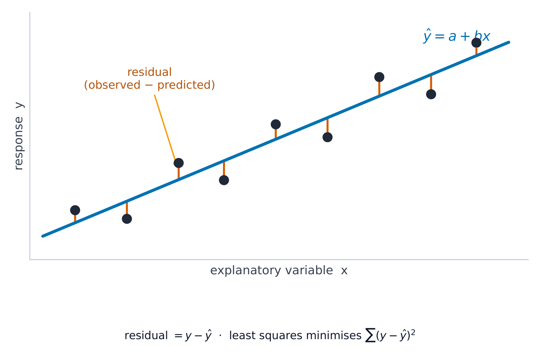
    The least-squares regression line 最小二乘回归线 predicts the response: $\hat{y}=a+bx$, where $\hat{y}$ is the predicted response. The slope 斜率 $b$ is the predicted change in $y$ per one-unit increase in $x$; the $y$-intercept 截距 $a$ is the predicted $y$ when $x=0$. Interpret both in context and with units – a graded skill. Avoid extrapolation 外推 (predicting far outside the data).

    Worked example. A study of hours studied ($x$) and test score ($y$) gives $\hat{y}=20+3x$. The slope means each extra hour of study is associated with a predicted $3$-point increase. A student who studies $5$ hours is predicted to score $\hat{y}=20+3(5)=35$.

    ไทย

    เส้นถดถอยกำลังน้อยที่สุด (least-squares regression line) ทำนายค่าตอบรับ: $\hat{y}=a+bx$, โดยที่ $\hat{y}$ คือ ค่าตอบรับที่ทำนาย. ความชัน $b$ คือการเปลี่ยนแปลงที่คาดหมายใน $y$ ต่อการเพิ่มขึ้นหนึ่งหน่วยใน $x$; จุดตัดแกน $y$ $a$ คือค่า $y$ ที่คาดหมายเมื่อ $x=0$. ตีความทั้งสอง ในบริบทและมีหน่วย – เป็นทักษะที่ต้องฝึกฝน หลีกเลี่ยง การ экстраโพลเลชัน (การทำนายไกลนอกข้อมูล)

    ตัวอย่างวิธีทำ. การศึกษาเกี่ยวกับชั่วโมงเรียน ($x$) และคะแนนทดสอบ ($y$) ได้ $\hat{y}=20+3x$. Slope หมายความว่าทุก额外的小时对应的 predicted increase of $3$ points. นักเรียนที่เรียน $5$ ชั่วโมง会被预测得分为 $\hat{y}=20+3(5)=35$.

    Explore · ⁨สำรวจ⁩

    Fit a least-squares line · ⁨ปรับเส้นน้อยที่สุดกำลังสอง⁩

    A regression line is the best straight-line fit, minimising the squared vertical distances. Its slope predicts how $y$ changes per unit of $x$. · ⁨เส้นถดถอย คือการปรับเส้นตรงที่ดีที่สุด โดยลดระยะทางแนวตั้งกำลังสองลง เส้นนี้ทำนายว่า $y$ จะเปลี่ยนไปเท่าไหร่ต่อหน่วยของ $x$⁩

    Vocabulary · ⁨คำศัพท์⁩ Train · ⁨ฝึกฝน⁩
    English ไทย
    least-squares regression line/liːst skweəz rɪˈɡreʃn laɪn/ เส้นถดถอยกำลังสองน้อยที่สุด
    slope/sləʊp/ ความชัน
    y-intercept/waɪ ˌɪntəˈsept/ จุดตัดแกน y
    extrapolation/ekˈstræpəleɪʃn/ การขยายนอกขอบเขตข้อมูล (extrapolation)
    2.7

    Residuals · ⁨ค่าคงเหลือ (Residuals)⁩

    Syllabus · ⁨หลักสูตร⁩
    English

    Enduring Understanding (DAT-1): Regression models may allow us to predict responses to changes in an explanatory variable.

    Learning Objective DAT-1.E: Represent differences between measured and predicted responses using residual plots. [Skill 2.B]

    • DAT-1.E.1 The residual is the difference between the actual value and the predicted value: $\text{residual} = y - \hat{y}$.
    • DAT-1.E.2 A residual plot is a plot of residuals versus explanatory variable values or predicted response values.

    Learning Objective DAT-1.F: Describe the form of association of bivariate data using residual plots. [Skill 2.A]

    • DAT-1.F.1 Apparent randomness in a residual plot for a linear model is evidence of a linear form to the association between the variables.
    • DAT-1.F.2 Residual plots can be used to investigate the appropriateness of a selected model.
    ไทย

    ความเข้าใจที่ยั่งยืน (DAT-1): แบบจำลองการถดถอยอาจช่วยให้เราทำนายผลลัพธ์จากการเปลี่ยนแปลงในตัวแปรอธิบายได้

    วัตถุประสงค์การเรียนรู้ DAT-1.E: แสดงความแตกต่างระหว่างค่าที่วัดได้และค่าที่คาดการณ์โดยใช้กราฟค่าคงเหลือ [ทักษะ 2.B]

    • DAT-1.E.1 ค่าคงเหลือคือความแตกต่างระหว่างค่าจริงและค่าที่คาดการณ์: $\text{residual} = y - \hat{y}$
    • DAT-1.E.2 กราฟค่าคงเหลือคือกราฟของค่าคงเหลือเทียบกับค่าของตัวแปรอธิบายหรือค่าที่คาดการณ์ของตัวแปรตอบสนอง

    วัตถุประสงค์การเรียนรู้ DAT-1.F: อธิบายรูปแบบของความสัมพันธ์ของข้อมูลเชิงปริมาณคู่โดยใช้กราฟค่าคงเหลือ [ทักษะ 2.A]

    • DAT-1.F.1 ความสุ่มที่ปรากฏในกราฟค่าคงเหลือสำหรับแบบจำลองเชิงเส้นเป็นหลักฐานของรูปแบบเชิงเส้นของความสัมพันธ์ระหว่างตัวแปร
    • DAT-1.F.2 กราฟค่าคงเหลือสามารถใช้เพื่อตรวจสอบความเหมาะสมของแบบจำลองที่เลือกไว้

    Source: College Board AP Course and Exam Description · ⁨แหล่งที่มา: คำอธิบายหลักสูตรและข้อสอบ College Board AP⁩

    English
    Least-squares regression

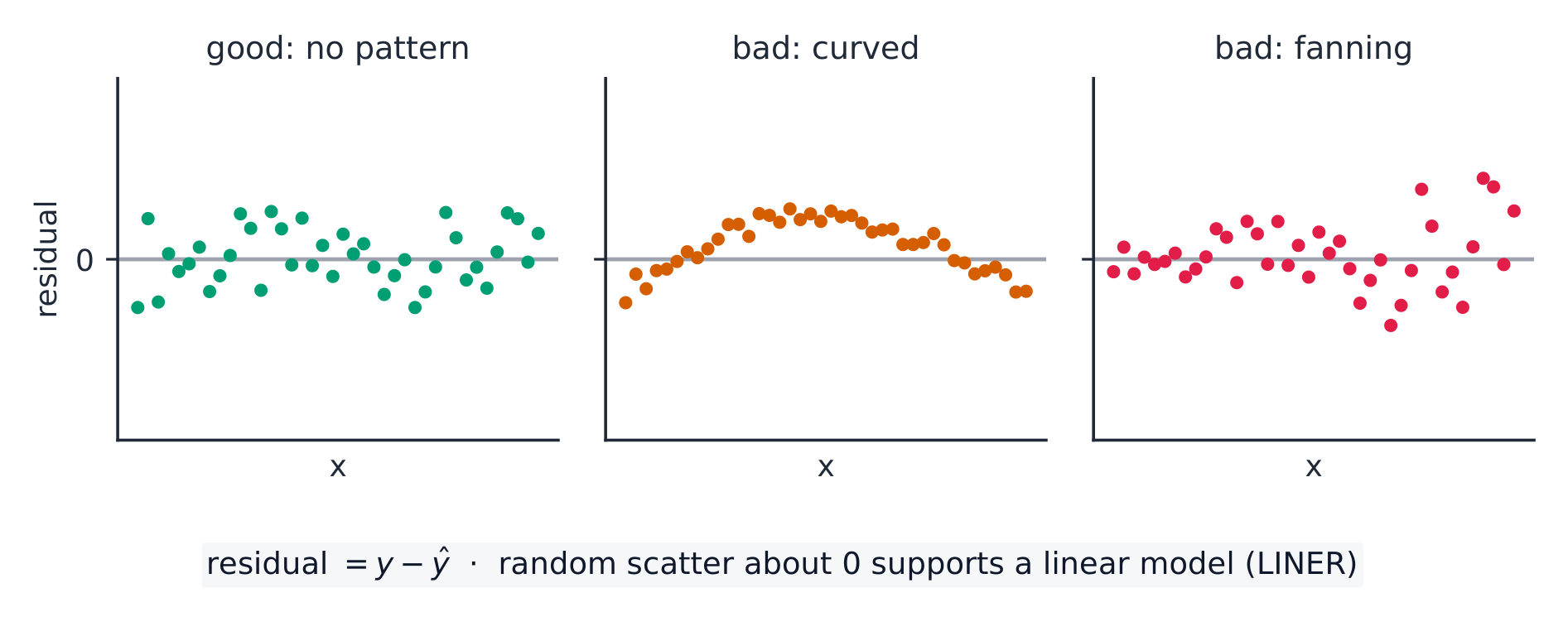
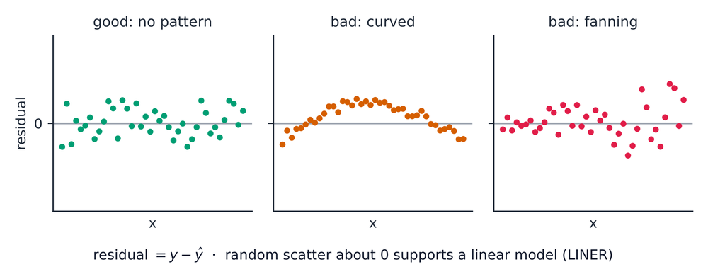
    A residual 残差 is actual minus predicted, $y-\hat{y}$: how far a point sits above (+) or below (−) the line. A residual plot 残差图 graphs residuals against $x$. If it shows no pattern (random scatter), a linear model is appropriate; a curved or fanning pattern means the linear model is a poor fit.

    Worked example. Continuing the study above, a student who studied $5$ hours actually scored $40$. The residual is $y-\hat{y}=40-35=+5$: the line under-predicted by $5$ points, so this point sits above the line.

    ไทย
    การถดถอยกำลังสองน้อยสุด (Least-squares regression)

    ค่าคงเหลือ (residual) คือจริงลบด้วยที่คาด, $y-\hat{y}$: ระยะห่างที่จุดอยู่เหนือ (+) หรือใต้ (−) เส้น. กราฟค่าคงเหลือ (residual plot) กราฟค่าคงเหลือเทียบกับ $x$. หากแสดง ไม่มีรูปแบบ (กระจัดกระจายแบบสุ่ม) โมเดลเชิงเส้นเหมาะสม; รูปแบบโค้งหรือแผ่ออกหมายความว่าโมเดลเชิงเส้นไม่พอดี

    ตัวอย่างคำนวณ. ต่อเนื่องจากการศึกษาข้างต้น นักเรียนที่เรียน $5$ ชั่วโมง ได้คะแนนจริง $40$. ค่าคงเหลือคือ $y-\hat{y}=40-35=+5$: เส้น ทำนายต่ำกว่า $5$ คะแนน, ดังนั้นจุดนี้อยู่เหนือเส้น

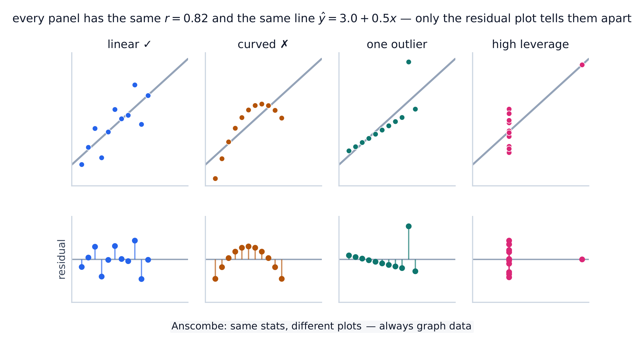
    ชุดข้อมูลสี่ชุดที่มี r และเส้นถดถอยเหมือนกันแต่มีรูปทรงต่างกันสี่แบบ
    ข้อควรระวังเกี่ยวกับ $r$ และเส้น: ชุดข้อมูลทั้งสี่มี $r=0.82$ และ $\hat{y}=3.0+0.5x$ เหมือนกัน แต่เพียงชุดแรกที่เป็นเชิงเส้นแท้จริง. กราฟกระจายแทบไม่แตกต่างกัน — กราฟค่าคงเหลือ ด้านล่างแต่ละชุดคือสิ่งที่เปิดเผยความโค้ง, ค่าสุดขั้ว, และจุดที่มีน้ำหนักสูง.
    Vocabulary · ⁨คำศัพท์⁩ Train · ⁨ฝึกฝน⁩
    English ไทย
    residual/rɪˈsɪdʒuːəl/ ค่าคงเหลือ
    residual plot/rɪˈsɪdʒuːəl plɒt/ แผนภูมิเศษเหลือ (residual plot)
    2.8

    Least-Squares Regression and Its Fit · ⁨การถดถอยกำลังน้อยที่สุดและการเข้ากันของโมเดล⁩

    Syllabus · ⁨หลักสูตร⁩
    English

    Enduring Understanding (DAT-1): Regression models may allow us to predict responses to changes in an explanatory variable.

    Learning Objective DAT-1.G: Estimate parameters for the least-squares regression line model. [Skill 2.C]

    • DAT-1.G.1 The least-squares regression model minimizes the sum of the squares of the residuals and contains the point $(\bar{x}, \bar{y})$.
    • DAT-1.G.2 The slope, $b$, of the regression line can be calculated as $b = r \left( \dfrac{s_y}{s_x} \right)$ where $r$ is the correlation between $x$ and $y$, $s_y$ is the sample standard deviation of the response variable, $y$, and $s_x$ is the sample standard deviation of the explanatory variable, $x$.
    • DAT-1.G.3 Sometimes, the $y$-intercept of the line does not have a logical interpretation in context.
    • DAT-1.G.4 In simple linear regression, $r^2$ is the square of the correlation, $r$. It is also called the coefficient of determination. $r^2$ is the proportion of variation in the response variable that is explained by the explanatory variable in the model.

    Learning Objective DAT-1.H: Interpret coefficients for the least-squares regression line model. [Skill 4.B]

    • DAT-1.H.1 The coefficients of the least-squares regression model are the estimated slope and $y$-intercept.
    • DAT-1.H.2 The slope is the amount that the predicted $y$-value changes for every unit increase in $x$.
    • DAT-1.H.3 The $y$-intercept value is the predicted value of the response variable when the explanatory variable is equal to $0$. The formula for the $y$-intercept, $a$, is $a = \bar{y} - b\bar{x}$.
    ไทย

    ความเข้าใจที่ยั่งยืน (DAT-1): แบบจำลองการถดถอยอาจช่วยให้เราทำนายผลลัพธ์จากการเปลี่ยนแปลงในตัวแปรอธิบายได้

    จุดประสงค์การเรียนรู้ DAT-1.G: ประมาณค่าพารามิเตอร์สำหรับโมเดลเส้นถดถอยกำลังน้อยที่สุด [ทักษะ 2.C]

    • DAT-1.G.1 โมเดลถดถอยกำลังน้อยที่สุดจะลดผลรวมของกำลังสองของความคลาดเคลื่อน (residuals) ลงให้ต่ำสุด และมีจุด $(\bar{x}, \bar{y})$ อยู่บนเส้น
    • DAT-1.G.2 ความชัน, $b$, ของเส้นถดถอยสามารถคำนวณได้จาก $b = r \left( \dfrac{s_y}{s_x} \right)$ โดยที่ $r$ คือสัมประสิทธิ์สหสัมพันธ์ระหว่าง $x$ และ $y$, $s_y$ คือส่วนเบี่ยงเบนมาตรฐานของตัวอย่างของตัวแปรตอบรับ, $y$, และ $s_x$ คือส่วนเบี่ยงเบนมาตรฐานของตัวอย่างของตัวแปรอธิบาย, $x$.
    • DAT-1.G.3 บางครั้ง ค่าตัดแกน $y$ ของเส้นอาจไม่มีความหมายในบริบทของปัญหา
    • DAT-1.G.4 ในสมการถดถอยเชิงเส้นอย่างง่าย, $r^2$ คือกำลังสองของสัมประสิทธิ์สหสัมพันธ์, $r$ มันยังเรียกว่าสัมประสิทธิ์การกำหนด $r^2$ เป็นสัดส่วนของความแปรปรวนในตัวแปรตอบรับที่ถูกอธิบายโดยตัวแปรอธิบายในโมเดล

    จุดประสงค์การเรียนรู้ DAT-1.H: ตีความสัมประสิทธิ์สำหรับโมเดลเส้นถดถอยกำลังน้อยที่สุด [ทักษะ 4.B]

    • DAT-1.H.1 สัมประสิทธิ์ของโมเดลถดถอยกำลังน้อยที่สุดคือความชันประมาณการและค่าตัดแกน $y$
    • DAT-1.H.2 ความชันคือปริมาณที่ค่า预测 $y$ เปลี่ยนแปลงไปสำหรับทุกหน่วยที่เพิ่มขึ้นของ $x$
    • DAT-1.H.3 ค่าตัดแกน $y$ คือค่า预测ของตัวแปรตอบรับเมื่อตัวแปรอธิบายมีค่าเท่ากับ $0$ สูตรสำหรับค่าตัดแกน $y$, $a$, คือ $a = \bar{y} - b\bar{x}$

    Source: College Board AP Course and Exam Description · ⁨แหล่งที่มา: คำอธิบายหลักสูตรและข้อสอบ College Board AP⁩

    English

    The line minimizes the sum of squared residuals. Its fit is measured by:

    • $s$, the standard deviation of the residuals – the typical prediction error, in the response's units.
    • $r^2$, the coefficient of determination 决定系数 – the proportion of the variation in $y$ that the linear model explains (a value between $0$ and $1$; multiply by $100$ to state it as a percent). Report it in context: "$r^2 = 0.81$ means 81% of the variation in $y$ is explained by the linear relationship with $x$."
    ไทย
    เส้นกำลังน้อยที่สุดลดผลรวมของค่าคงเหลือยกกำลังสองให้ต่ำสุด
    เส้นกำลังน้อยที่สุดลดผลรวมของค่าคงเหลือยกกำลังสองให้ต่ำสุด

    เส้นลดผลรวมของค่าคงเหลือยกกำลังสองให้ต่ำสุด การเข้ากันวัดโดย:

    • $s$, ส่วนเบี่ยงเบนมาตรฐานของค่าคงเหลือ – ความผิดพลาดในการคาดหมายทั่วไป, ในหน่วยของค่าตอบรับ.
    • $r^2$, สัมประสิทธิ์การกำหนด (coefficient of determination) – สัดส่วนของความแปรปรวนใน $y$ ที่โมเดลเชิงเส้นอธิบาย (ค่าระหว่าง $0$ และ $1$; คูณด้วย $100$ เพื่อระบุเป็นเปอร์เซ็นต์). รายงานในบริบท: "$r^2 = 0.81$ หมายถึง 81% ของความแปรปรวนใน $y$ ถูกอธิบายด้วยความสัมพันธ์เชิงเส้นกับ $x$."
    Vocabulary · ⁨คำศัพท์⁩ Train · ⁨ฝึกฝน⁩
    English ไทย
    coefficient of determination/ˌkəʊɪˈfɪʃənt ɒv dɪˌtɜːmɪˈneɪʃn/ สัมประสิทธิ์การกำหนด (coefficient of determination)
    2.9

    Departures from Linearity · ⁨ความเบี่ยงเบนจากความเป็นเชิงเส้น⁩

    Syllabus · ⁨หลักสูตร⁩
    English

    Enduring Understanding (DAT-1): Regression models may allow us to predict responses to changes in an explanatory variable.

    Learning Objective DAT-1.I: Identify influential points in regression. [Skill 2.A]

    • DAT-1.I.1 An outlier in regression is a point that does not follow the general trend shown in the rest of the data and has a large residual when the Least Squares Regression Line (LSRL) is calculated.
    • DAT-1.I.2 A high-leverage point in regression has a substantially larger or smaller $x$-value than the other observations have.
    • DAT-1.I.3 An influential point in regression is any point that, if removed, changes the relationship substantially. Examples include much different slope, $y$-intercept, and/or correlation. Outliers and high leverage points are often influential.

    Learning Objective DAT-1.J: Calculate a predicted response using a least-squares regression line for a transformed data set. [Skill 2.C]

    • DAT-1.J.1 Transformations of variables, such as evaluating the natural logarithm of each value of the response variable or squaring each value of the explanatory variable, can be used to create transformed data sets, which may be more linear in form than the untransformed data.
    • DAT-1.J.2 Increased randomness in residual plots after transformation of data and/or movement of $r^2$ to a value closer to 1 offers evidence that the least-squares regression line for the transformed data is a more appropriate model to use to predict responses to the explanatory variable than the regression line for the untransformed data.
    ไทย

    ความเข้าใจที่ยั่งยืน (DAT-1): แบบจำลองการถดถอยอาจช่วยให้เราทำนายผลลัพธ์จากการเปลี่ยนแปลงในตัวแปรอธิบายได้

    จุดประสงค์การเรียนรู้ DAT-1.I: ชนจุดที่มีอิทธิพลในการถดถอย [ทักษะ 2.A]

    • DAT-1.I.1 จุดผิดปกติ (outlier) ในการถดถอยคือจุดที่ไม่สอดคล้องกับแนวโน้มทั่วไปที่แสดงอยู่ในข้อมูลส่วนที่เหลือและมีค่าความคลาดเคลื่อนสูงเมื่อคำนวณเส้นถดถอยกำลังน้อยที่สุด (LSRL)
    • DAT-1.I.2 จุดที่มีอำนาจสูง (high-leverage point) ในการถดถอยมีค่า $x$ ที่แตกต่างกันอย่างมากหรือมากกว่า/น้อยกว่าจุดสังเกตอื่นๆ อย่างชัดเจน
    • DAT-1.I.3 จุดที่มีอิทธิพล (influential point) ในการถดถอยคือจุดใดๆ ที่หากถูกนำออก จะทำให้ความสัมพันธ์เปลี่ยนแปลงไปอย่างมาก ตัวอย่างเช่น ความชัน, ค่าตัดแกน $y$, และ/หรือ สัมประสิทธิ์สหสัมพันธ์ที่แตกต่างกันมาก จุดผิดปกติและจุดที่มีอำนาจสูงมักจะมีอิทธิพล

    จุดประสงค์การเรียนรู้ DAT-1.J: คำนวณค่า predicted response โดยใช้เส้นถดถอยกำลังน้อยที่สุดสำหรับชุดข้อมูลที่แปลงแล้ว [ทักษะ 2.C]

    • DAT-1.J.1 การแปลงตัวแปร เช่น การหาค่าลอการิทึมธรรมชาติของแต่ละค่าของตัวแปรตอบรับ หรือการยกกำลังสองของแต่ละค่าของตัวแปรอธิบาย สามารถใช้เพื่อสร้างชุดข้อมูลที่แปลงแล้ว ซึ่งอาจมีความเป็นเชิงเส้นมากกว่าข้อมูลที่ไม่ได้แปลง
    • DAT-1.J.2 ความสุ่มที่เพิ่มขึ้นในกราฟความคลาดเคลื่อนหลังการแปลงข้อมูลและ/หรือการเคลื่อนย้าย $r^2$ ไปสู่ค่าที่ใกล้ 1 มากขึ้น เป็นหลักฐานว่าเส้นถดถอยกำลังน้อยที่สุดสำหรับข้อมูลที่ได้แปลงแล้วเป็นโมเดลที่เหมาะสมกว่าในการ predict responses ต่อตัวแปรอธิบาย เมื่อเทียบกับเส้นถดถอยสำหรับข้อมูลที่ไม่ได้แปลง

    Source: College Board AP Course and Exam Description · ⁨แหล่งที่มา: คำอธิบายหลักสูตรและข้อสอบ College Board AP⁩

    English

    Some points strongly affect the line. A high-leverage 高杠杆 point has an extreme $x$-value; an influential 有影响的 point noticeably changes the slope or $r$ when removed; an outlier here is a point with a large residual. When the pattern is curved, transform a variable (e.g. take a log) to straighten it, then fit a line to the transformed data.

    ไทย

    บางจุดส่งผลต่อเส้นอย่างมาก จุด น้ำหนักสูง (high-leverage) มีค่า $x$ ที่สุดขั้ว; จุด มีอิทธิพล (influential) เปลี่ยนความชันหรือ $r$ อย่างชัดเจนเมื่อถูกเอาออก; ค่าสุดขั้ว (outlier)在这里 คือจุดที่มีค่าคงเหลือใหญ่. เมื่อรูปแบบเป็นโค้ง ให้ แปลง ตัวแปร (เช่นTaking a log) เพื่อให้เป็นเส้นตรง แล้วปรับเส้นเข้ากับข้อมูลที่แปลงแล้ว

    Vocabulary · ⁨คำศัพท์⁩ Train · ⁨ฝึกฝน⁩
    English ไทย
    high-leverage/haɪ ˈliːvərɪdʒ/ จุดที่มีอิทธิพลสูง (high-leverage)
    influential/ˌɪnfluːˈenʃl/ มีอิทธิพล (influential)
    2.9

    Exam tips · ⁨ข้อแนะนำสำหรับการสอบ⁩

    English
    • On a scatterplot describe direction, form, strength, and outliers; $r$ ranges $-1$ to $1$.
    • Correlation is not causation — a lurking variable can drive both.
    • Interpret the slope of the least-squares line in context ("per one unit of $x$, predicted $y$ changes by $b$").
    • Check a residual plot: no pattern means a line fits; a curve means it does not. Avoid extrapolation.
    • $r^2$ is the fraction of variation in $y$ explained by the model.
    ไทย
    • บนกราฟกระจาย อธิบาย ทิศทาง, รูปแบบ, ความเข้ม, และค่าสุดขั้ว; $r$ มีช่วง $-1$ ถึง $1$.
    • สหสัมพันธ์ไม่ใช่สาเหตุ – ตัวแปรแฝงอาจขับเคลื่อนทั้งสองอย่าง
    • ตีความความชันของเส้นกำลังน้อยที่สุดในบริบท ("ต่อหนึ่งหน่วยของ $x$, ค่า $y$ ที่คาดเปลี่ยนไป $b$").
    • ตรวจสอบ กราฟค่าคงเหลือ: ไม่มีแปลว่าเส้นเข้ากัน; เป็นโค้งแปลว่าไม่เข้ากัน. หลีกเลี่ยงการ ekstrapolation
    • $r^2$ คือสัดส่วนของความแปรปรวนใน $y$ ที่โมเดลอธิบายได้
  • 3

    Collecting Data · ⁨การเก็บรวบรวมข้อมูล⁩

    Watch lesson · ⁨ดูบทเรียน⁩
    3.1

    Can We Trust the Data We Collected? · ⁨เราเชื่อถือข้อมูลที่เก็บรวบรวมได้หรือไม่?⁩

    Syllabus · ⁨หลักสูตร⁩
    English

    Enduring Understanding (VAR-1): Given that variation may be random or not, conclusions are uncertain.

    Learning Objective VAR-1.E: Identify questions to be answered about data collection methods. [Skill 1.A]

    • VAR-1.E.1 Methods for data collection that do not rely on chance result in untrustworthy conclusions.
    ไทย

    ความเข้าใจที่ยั่งยืน (VAR-1): เนื่องจากความแปรปรวนอาจเป็นแบบสุ่มหรือไม่ ดังนั้นข้อสรุปจึงมีความไม่แน่นอน

    จุดประสงค์การเรียนรู้ VAR-1.E: ระบุคำถามที่ต้องการตอบเกี่ยวกับวิธีการเก็บข้อมูล [ทักษะ 1.A]

    • VAR-1.E.1 วิธีการเก็บข้อมูลที่ไม่อาศัยโอกาสจะนำไปสู่ข้อสรุปที่เชื่อถือไม่ได้

    Source: College Board AP Course and Exam Description · ⁨แหล่งที่มา: คำอธิบายหลักสูตรและข้อสอบ College Board AP⁩

    English

    A conclusion is only as good as the data behind it. How data are collected decides what you may conclude – whether you can generalize to a population 总体, and whether you can claim cause and effect. Poorly collected data can be worse than none.

    ไทย

    ข้อสรุปดีเท่ากับข้อมูลที่อยู่เบื้องหลัง. วิธีการ เก็บข้อมูลกำหนดสิ่งที่คุณจะสรุปได้ – whether you can generalizing to a ประชากร, and whether you can claim เหตุและผล. ข้อมูลที่เก็บไม่ดีอาจแย่กว่าไม่มีเลย

    3.2

    Observational Studies and Experiments · ⁨การศึกษาเชิงสังเกตและการทดลอง⁩

    Syllabus · ⁨หลักสูตร⁩
    English

    Enduring Understanding (DAT-2): The way we collect data influences what we can and cannot say about a population.

    Learning Objective DAT-2.A: Identify the type of a study. [Skill 1.C]

    • DAT-2.A.1 A population consists of all items or subjects of interest.
    • DAT-2.A.2 A sample selected for study is a subset of the population.
    • DAT-2.A.3 In an observational study, treatments are not imposed. Investigators examine data for a sample of individuals (retrospective) or follow a sample of individuals into the future collecting data (prospective) in order to investigate a topic of interest about the population. A sample survey is a type of observational study that collects data from a sample in an attempt to learn about the population from which the sample was taken.
    • DAT-2.A.4 In an experiment, different conditions (treatments) are assigned to experimental units (participants or subjects).

    Learning Objective DAT-2.B: Identify appropriate generalizations and determinations based on observational studies. [Skill 4.A]

    • DAT-2.B.1 It is only appropriate to make generalizations about a population based on samples that are randomly selected or otherwise representative of that population.
    • DAT-2.B.2 A sample is only generalizable to the population from which the sample was selected.
    • DAT-2.B.3 It is not possible to determine causal relationships between variables using data collected in an observational study.
    ไทย

    ความเข้าใจที่ยั่งยืน (DAT-2): วิธีการที่เราเก็บข้อมูลมีผลต่อสิ่งที่เราสามารถพูดและไม่สามารถพูดเกี่ยวกับประชากรได้

    จุดประสงค์การเรียนรู้ DAT-2.A: ระบุประเภทของการศึกษา [ทักษะ 1.C]

    • DAT-2.A.1 ประชากรประกอบด้วยวัตถุหรือ Subjects ทั้งหมดที่เกี่ยวข้อง
    • DAT-2.A.2 ตัวอย่างที่เลือกสำหรับการศึกษาเป็นSubset ของประชากร
    • DAT-2.A.3 ในการศึกษาแบบสังเกต (observational study), การทดลอง (treatments) ไม่ถูกบังคับ นักวิจัยตรวจสอบข้อมูลจากกลุ่มตัวอย่างของบุคคล (retrospective) หรือติดตามกลุ่มตัวอย่างของบุคคลเข้าสู่อนาคตเพื่อเก็บข้อมูล (prospective) เพื่อศึกษาหัวข้อที่น่าสนใจเกี่ยวกับประชากร การสำรวจตัวอย่าง (sample survey) เป็นประเภทหนึ่งของการศึกษาแบบสังเกตที่เก็บข้อมูลจากตัวอย่างเพื่อพยายามเรียนรู้เกี่ยวกับประชากรที่ตัวอย่างนั้นถูกดึงมาจากนั้น
    • DAT-2.A.4 ในการทดลอง (experiment), เงื่อนไขต่างๆ (treatments) ถูกกำหนดให้กับหน่วยทดลอง (experimental units) (ผู้เข้าร่วมหรือ subjects)

    จุดประสงค์การเรียนรู้ DAT-2.B: ระบุการสรุปและการตัดสินที่เหมาะสมจากการศึกษาแบบสังเกต [ทักษะ 4.A]

    • DAT-2.B.1 เหมาะสมที่จะสรุปเกี่ยวกับประชากรได้ก็ต่อเมื่อตัวอย่างถูกสุ่มเลือกหรือเป็นตัวแทนของประชากรนั้น
    • DAT-2.B.2 ตัวอย่างสามารถสรุปไปยังประชากรได้ก็ต่อเมื่อประชากรนั้นเป็นประชากรที่ตัวอย่างถูกเลือกออกมาจากเท่านั้น
    • DAT-2.B.3 เป็นไปไม่ได้ที่จะระบุความสัมพันธ์เชิงสาเหตุระหว่างตัวแปรโดยใช้ข้อมูลที่เก็บมาจากการศึกษาแบบสังเกต

    Source: College Board AP Course and Exam Description · ⁨แหล่งที่มา: คำอธิบายหลักสูตรและข้อสอบ College Board AP⁩

    English
    • In an observational study 观察性研究 you measure individuals without trying to influence them. It can show association, but not causation, because lurking variables may explain the link.
    • In an experiment 实验 you deliberately impose a treatment 处理 and compare responses. A well-designed experiment can establish cause and effect.
    ไทย
    • ในการ การศึกษาเชิงสังเกต คุณวัดบุคคลโดยไม่พยายามส่งผลกระทบ. สามารถแสดง ความสัมพันธ์, แต่ไม่ใช่สาเหตุ, เพราะตัวแปรแฝงอาจอธิบายความเชื่อมโยง
    • ในการ การทดลอง คุณกำหนด การรักษา (treatment) อย่างตั้งใจและเปรียบเทียบคำตอบ. การทดลองที่ออกแบบดี สามารถ สร้างเหตุผลและผลได้
    Explore · ⁨สำรวจ⁩

    Observational study or experiment? · ⁨การศึกษารายละเอียดหรือการทดลอง?⁩

    In an experiment the researcher imposes a treatment (and can show cause); an observational study only records what already happens (and can show association, not cause). · ⁨ในการ ทดลอง นักวิจัย กำหนด การรักษา (และสามารถพิสูจน์เหตุและผลได้); การศึกษารายละเอียด บันทึกเพียงสิ่งที่เกิดขึ้นอยู่แล้ว (และสามารถแสดงความสัมพันธ์ แต่ไม่ใช่เหตุและผล)⁩

    Vocabulary · ⁨คำศัพท์⁩ Train · ⁨ฝึกฝน⁩
    English ไทย
    treatment/ˈtriːtmənt/ การรักษา
    sample/ˈsæmpl/ ตัวอย่าง
    Random sampling/ˈrændəm ˈsæmplɪŋ/ การสุ่มตัวอย่าง
    3.3

    Random Sampling · ⁨การสุ่มตัวอย่าง⁩

    Syllabus · ⁨หลักสูตร⁩
    English

    Enduring Understanding (DAT-2): The way we collect data influences what we can and cannot say about a population.

    Learning Objective DAT-2.C: Identify a sampling method, given a description of a study. [Skill 1.C]

    • DAT-2.C.1 When an item from a population can be selected only once, this is called sampling without replacement. When an item from the population can be selected more than once, this is called sampling with replacement.
    • DAT-2.C.2 A simple random sample (SRS) is a sample in which every group of a given size has an equal chance of being chosen. This method is the basis for many types of sampling mechanisms. A few examples of mechanisms used to obtain SRSs include numbering individuals and using a random number generator to select which ones to include in the sample, ignoring repeats, using a table of random numbers, or drawing a card from a deck without replacement.
    • DAT-2.C.3 A stratified random sample involves the division of a population into separate groups, called strata, based on shared attributes or characteristics (homogeneous grouping). Within each stratum a simple random sample is selected, and the selected units are combined to form the sample.
    • DAT-2.C.4 A cluster sample involves the division of a population into smaller groups, called clusters. Ideally, there is heterogeneity within each cluster, and clusters are similar to one another in their composition. A simple random sample of clusters is selected from the population to form the sample of clusters. Data are collected from all observations in the selected clusters.
    • DAT-2.C.5 A systematic random sample is a method in which sample members from a population are selected according to a random starting point and a fixed, periodic interval.
    • DAT-2.C.6 A census selects all items/subjects in a population.

    Learning Objective DAT-2.D: Explain why a particular sampling method is or is not appropriate for a given situation. [Skill 1.C]

    • DAT-2.D.1 There are advantages and disadvantages for each sampling method depending upon the question that is to be answered and the population from which the sample will be drawn.
    ไทย

    ความเข้าใจที่ยั่งยืน (DAT-2): วิธีการที่เราเก็บข้อมูลมีผลต่อสิ่งที่เราสามารถพูดและไม่สามารถพูดเกี่ยวกับประชากรได้

    จุดประสงค์การเรียนรู้ DAT-2.C: ระบุวิธีการสุ่มตัวอย่าง จากคำอธิบายของการศึกษา [ทักษะ 1.C]

    • DAT-2.C.1 เมื่อวัตถุจากประชากรสามารถถูกเลือกได้เพียงครั้งเดียว เรียกว่าการสุ่มโดยไม่แทนที่ (sampling without replacement) เมื่อวัตถุจากประชากรสามารถถูกเลือกได้มากกว่าครั้งเดียว เรียกว่าการสุ่มโดยแทนที่ (sampling with replacement)
    • DAT-2.C.2 ตัวอย่างสุ่มอย่างง่าย (SRS) เป็นตัวอย่างที่แต่ละกลุ่มที่มีขนาดที่กำหนดมีโอกาสเท่าๆ กันที่จะถูกเลือก วิธีนี้เป็นพื้นฐานของกลไกการสุ่มหลายชนิด ตัวอย่างของกลไกที่ใช้ในการได้ SRSs รวมถึงการให้หมายเลขแก่บุคคลและการใช้เครื่องสุ่มตัวเลขเพื่อเลือก哪些 who should be included in the sample, ignoring repeats, using a table of random numbers, or drawing a card from a deck without replacement.
    • DAT-2.C.3 การสุ่มตัวอย่างแบบแบ่งชั้น (stratified random sample) เกี่ยวข้องกับการแบ่งประชากรออกเป็นกลุ่มย่อยที่แยกจากกัน ซึ่งเรียกว่า ชั้น (strata) โดยพิจารณาตามคุณสมบัติหรือลักษณะร่วม (การจับกลุ่มที่มีลักษณะคล้ายคลึงกัน) ภายในแต่ละชั้นจะทำการสุ่มตัวอย่างแบบง่าย และนำหน่วยตัวอย่างที่เลือกมามารวมกันเพื่อสร้างเป็นตัวอย่าง
    • DAT-2.C.4 การสุ่มตัวอย่างแบบกลุ่ม (cluster sample) เกี่ยวข้องกับการแบ่งประชากรออกเป็นกลุ่มย่อยที่เล็กกว่า ซึ่งเรียกว่า กลุ่ม (clusters) ในทาง理想的แล้ว ควรมีความหลากหลายภายในแต่ละกลุ่ม และกลุ่มต่างๆ ควรมีองค์ประกอบคล้ายคลึงกันกับอีกกลุ่มหนึ่งๆ จะสุ่มตัวอย่างแบบง่ายจากกลุ่มของประชากรเพื่อสร้างเป็นตัวอย่างของกลุ่ม ข้อมูลจะถูกเก็บรวบรวมจากทุกข้อสังเกตในกลุ่มที่ถูกเลือก
    • DAT-2.C.5 การสุ่มตัวอย่างแบบมีระบบ (systematic random sample) เป็นวิธีการที่สมาชิกตัวอย่างจากประชากรถูกเลือกโดยเริ่มจากจุดเริ่มต้นแบบสุ่ม และมีช่วงระยะคงที่ตามกำหนด
    • DAT-2.C.6 การสำมะโน (census) เลือกตัว物件/ Subjects ทั้งหมดในประชากร

    วัตถุประสงค์การเรียนรู้ DAT-2.D: อธิบายเหตุผลว่าทำไมวิธีการสุ่มตัวอย่างแบบใดแบบหนึ่งจึงเหมาะสมหรือไม่เหมาะสมสำหรับสถานการณ์ที่กำหนด [ทักษะ 1.C]

    • DAT-2.D.1 แต่ละวิธีการสุ่มตัวอย่างมีทั้งข้อดีและข้อเสียขึ้นอยู่กับคำถามที่ต้องการตอบและประชากรที่จะดึงตัวอย่างออกมา

    Source: College Board AP Course and Exam Description · ⁨แหล่งที่มา: คำอธิบายหลักสูตรและข้อสอบ College Board AP⁩

    English

    To learn about a population you take a sample 样本. Random sampling 随机抽样 protects against selection bias 偏差 and lets you generalize (it cannot fix undercoverage, nonresponse, or response bias — see below). Common designs:

    • Simple random sample (SRS) 简单随机样本: every group of the chosen size is equally likely.
    • Stratified 分层: split the population into similar strata, then sample within each.
    • Cluster 整群: split into clusters, randomly choose whole clusters.
    • Systematic 系统: pick every $k$th individual from a random start.

    A convenience sample 方便样本 or voluntary response sample is not random and is biased.

    Worked example. To survey a school, an administrator lists all students by grade and randomly selects $20$ from each grade. This is a stratified sample – the grades are the strata – which guarantees every grade is represented, unlike an SRS that might by chance draw few from one grade.

    ไทย

    เพื่อเรียนรู้เกี่ยวกับประชากรคุณต้อง取了 ตัวอย่าง. การสุ่มตัวอย่าง ป้องกัน อคติ ในการเลือกและทำให้คุณสามารถ generalize (มันไม่สามารถแก้ไข undercoverage, nonresponse, หรือ response bias – ดูด้านล่าง). แบบแผนทั่วไป:

    • ตัวอย่างสุ่มง่าย (SRS): ทุกกลุ่มขนาดที่เลือกมีความน่าจะเป็นเท่ากัน
    • แบบแบ่งชั้น: แบ่งประชากรเป็นชั้นที่คล้ายกัน, แล้วสุ่มภายในแต่ละชั้น
    • แบบกลุ่ม: แบ่งเป็นกลุ่ม, เลือกทั้งกลุ่มแบบสุ่ม
    • แบบระบบ: เลือกทุก $k$-nth บุคคลจากรandom start
    สี่แบบแผนการสุ่มตัวอย่าง: ใครได้รับคัดเลือก, และอย่างไร
    การออกแบบการสุ่มตัวอย่างแบบสุ่มสี่แบบ: ใครถูกเลือก และ چگونه

    ตัวอย่างความสะดวก หรือ ตัวอย่างการตอบสนองโดยสมัครใจ เป็น ไม่ใช่ แบบสุ่มและมี ความลำเอียง

    ตัวอย่างที่แสดงวิธีทำ. เพื่อสำรวจโรงเรียน ผู้บริหารจัดรายชื่อนักเรียนตามระดับชั้นและสุ่มเลือก $20$ จากแต่ละระดับชั้น นี่คือ ตัวอย่างแบบแบ่งชั้น – ระดับชั้นคือชั้น stratification – ซึ่งรับประกันว่าทุกระดับชั้นมีตัวแทนต่างจาก SRS ที่อาจโดยบังเอิญดึงตัวอย่างน้อยจากระดับชั้นใดระดับชั้นหนึ่ง

    ผลลัพธ์แบบสุ่ม: ลูกเต๋าทำให้แต่ละหน้ามีโอกาสเท่ากันภายใต้เงื่อนไขที่ยุติธรรม
    ผลลัพธ์แบบสุ่ม: ลูกเต๋าทำให้แต่ละหน้ามีโอกาสเท่ากันภายใต้เงื่อนไขที่ยุติธรรม
    Vocabulary · ⁨คำศัพท์⁩ Train · ⁨ฝึกฝน⁩
    English ไทย
    bias/ˈbaɪəs/ อคติ
    Simple random sample (SRS)/ˈsɪmpl ˈrændəm ˈsæmpl/ ตัวอย่างสุ่มอย่างง่าย (SRS)
    Stratified/ˈstrætɪfaɪd/ Stratified
    Cluster/ˈklʌstə/ Cluster
    Systematic/ˌsɪstəˈmætɪk/ Systematic
    convenience sample/kənˈviːnɪəns ˈsæmpl/ ตัวอย่างแบบสะดวก
    Undercoverage/ˌʌndəˈkʌvərɪdʒ/ การครอบคลุมไม่เพียงพอ (Undercoverage)
    Nonresponse/ˌnɒnrɪˈspɒns/ การไม่ตอบคำถาม
    Response bias/rɪˈspɒns ˈbaɪəs/ ความเบี่ยงเบนจากการตอบคำถาม
    control group/kənˈtrəʊl ɡruːp/ กลุ่มควบคุม (control group)
    placebo/pləˈsiːbəʊ/ ยาหลอกลวง
    Random assignment/ˈrændəm əˈsaɪnmənt/ การจัดกลุ่มแบบสุ่ม
    Replication/ˌreplɪˈkeɪʃn/ การทำซ้ำ (Replication)
    Confounding/kənˈfaʊndɪŋ/ ตัวแปรรบกวน (Confounding)
    Blinding/ˈblaɪndɪŋ/ การบดบัง
    single-blind/ˈsɪŋɡl blaɪnd/ บอดแบบฝ่ายเดียว (single-blind)
    double-blind/ˈdʌbl blaɪnd/ บอดแบบสองฝ่าย (double-blind)
    Blocking/ˈblɒkɪŋ/ การจัดกลุ่มตัวแปร
    3.4

    When Sampling Goes Wrong · ⁨เมื่อการสุ่มตัวอย่างผิดพลาด⁩

    Syllabus · ⁨หลักสูตร⁩
    English

    Enduring Understanding (DAT-2): The way we collect data influences what we can and cannot say about a population.

    Learning Objective DAT-2.E: Identify potential sources of bias in sampling methods. [Skill 1.C]

    • DAT-2.E.1 Bias occurs when certain responses are systematically favored over others.
    • DAT-2.E.2 When a sample is comprised entirely of volunteers or people who choose to participate, the sample will typically not be representative of the population (voluntary response bias).
    • DAT-2.E.3 When part of the population has a reduced chance of being included in the sample, the sample will typically not be representative of the population (undercoverage bias).
    • DAT-2.E.4 Individuals chosen for the sample for whom data cannot be obtained (or who refuse to respond) may differ from those for whom data can be obtained (nonresponse bias).
    • DAT-2.E.5 Problems in the data gathering instrument or process result in response bias. Examples include questions that are confusing or leading (question wording bias) and self-reported responses.
    • DAT-2.E.6 Non-random sampling methods (for example, samples chosen by convenience or voluntary response) introduce potential for bias because they do not use chance to select the individuals.
    ไทย

    ความเข้าใจที่ยั่งยืน (DAT-2): วิธีการที่เราเก็บข้อมูลมีผลต่อสิ่งที่เราสามารถพูดและไม่สามารถพูดเกี่ยวกับประชากรได้

    วัตถุประสงค์การเรียนรู้ DAT-2.E: ระบุแหล่งที่มาที่เป็นไปได้ของความเบี่ยงเบน (bias) ในวิธีการสุ่มตัวอย่าง [ทักษะ 1.C]

    • DAT-2.E.1 ความเบี่ยงเบนเกิดขึ้นเมื่อคำตอบบางประเภทถูกสนับสนุนอย่างเป็นระบบมากกว่าอีกประเภทหนึ่ง
    • DAT-2.E.2 เมื่อตัวอย่างประกอบด้วยผู้สมัครใจทั้งหมดหรือคนที่เลือกเข้าร่วม ตัวอย่างนั้นมักจะไม่เป็นตัวแทนของประชากร (ความเบี่ยงเบนจากการตอบแบบสมัครใจ - voluntary response bias)
    • DAT-2.E.3 เมื่อส่วนหนึ่งของประชากรมีโอกาสถูกนำเข้าสู่ตัวอย่างลดลง ตัวอย่างนั้นมักจะไม่เป็นตัวแทนของประชากร (ความเบี่ยงเบนจากการครอบคลุมไม่เพียงพอ - undercoverage bias)
    • DAT-2.E.4 บุคคลที่ถูกเลือกเข้าตัวอย่างซึ่งไม่สามารถเก็บข้อมูลได้ (หรือปฏิเสธที่จะตอบ) อาจแตกต่างจากผู้ที่สามารถเก็บข้อมูลได้ (ความเบี่ยงเบนจากการไม่ตอบกลับ - nonresponse bias)
    • DAT-2.E.5 ปัญหาในเครื่องมือหรือกระบวนการเก็บรวบรวมข้อมูลส่งผลให้เกิดความเบี่ยงเบนในการตอบ ตัวอย่างเช่น คำถามที่สับสนหรือชี้นำ (ความเบี่ยงเบนจากรูปแบบคำถาม - question wording bias) และการตอบด้วยตนเอง
    • DAT-2.E.6 วิธีการสุ่มตัวอย่างที่ไม่ได้สุ่ม (เช่น การเลือกตัวอย่างตามความสะดวกหรือการตอบแบบสมัครใจ) นำไปสู่ความเป็นไปได้ของความเบี่ยงเบนเพราะไม่ได้ใช้โอกาสในการเลือกบุคคล

    Source: College Board AP Course and Exam Description · ⁨แหล่งที่มา: คำอธิบายหลักสูตรและข้อสอบ College Board AP⁩

    English

    Bias makes estimates systematically miss the truth:

    • Undercoverage 覆盖不足: some groups are left out of the sampling frame.
    • Nonresponse 无回应: selected people do not answer.
    • Response bias 回应偏差: people answer inaccurately (bad wording, sensitive topics).

    Bias is about a consistent error in one direction – increasing the sample size does not fix it.

    ไทย

    ความลำเอียง ทำให้ค่าประมาณคลาดเคลื่อนจากความจริงอย่างมีระบบ:

    • การครอบคลุมไม่เพียงพอ: กลุ่มบางกลุ่มถูกตัดออกจากกรอบการสุ่มตัวอย่าง
    • การไม่ตอบกลับ: บุคคลที่ถูกเลือกไม่ตอบคำถาม
    • ความลำเอียงจากการตอบกลับ: ผู้ตอบตอบไม่ถูกต้อง (การตั้งคำถามที่ไม่ดี, หัวข้อที่อ่อนไหว)

    ความลำเอียงเป็นเรื่องของ ความคลาดเคลื่อนที่สม่ำเสมอ ในทิศทางใดทิศทางหนึ่ง – การเพิ่มขนาดตัวอย่างไม่ได้แก้ปัญหา

    ตัวอย่างความสะดวกขาดจากประชากร: ความลำเอียงแทรกซึมเข้ามาเมื่อการคัดเลือกไม่เป็นแบบสุ่ม
    ตัวอย่างความสะดวกขาดจากประชากร: ความลำเอียงแทรกซึมเข้ามาเมื่อการคัดเลือกไม่เป็นแบบสุ่ม
    3.5

    Designing an Experiment · ⁨การออกแบบการทดลอง⁩

    Syllabus · ⁨หลักสูตร⁩
    English

    Enduring Understanding (VAR-3): Well-designed experiments can establish evidence of causal relationships.

    Learning Objective VAR-3.A: Identify the components of an experiment. [Skill 1.C]

    • VAR-3.A.1 The experimental units are the individuals (which may be people or other objects of study) that are assigned treatments. When experimental units consist of people, they are sometimes referred to as participants or subjects.
    • VAR-3.A.2 An explanatory variable (or factor) in an experiment is a variable whose levels are manipulated intentionally. The levels or combination of levels of the explanatory variable(s) are called treatments.
    • VAR-3.A.3 A response variable in an experiment is an outcome from the experimental units that is measured after the treatments have been administered.
    • VAR-3.A.4 A confounding variable in an experiment is a variable that is related to the explanatory variable and influences the response variable and may create a false perception of association between the two.

    Learning Objective VAR-3.B: Describe elements of a well-designed experiment. [Skill 1.B]

    • VAR-3.B.1 A well-designed experiment should include the following:
      • a. Comparisons of at least two treatment groups, one of which could be a control group.
      • b. Random assignment/allocation of treatments to experimental units.
      • c. Replication (more than one experimental unit in each treatment group).
      • d. Control of potential confounding variables where appropriate.

    Learning Objective VAR-3.C: Compare experimental designs and methods. [Skill 1.C]

    • VAR-3.C.1 In a completely randomized design, treatments are assigned to experimental units completely at random. Random assignment tends to balance the effects of uncontrolled (confounding) variables so that differences in responses can be attributed to the treatments.
    • VAR-3.C.2 Methods for randomly assigning treatments to experimental units in a completely randomized design include using a random number generator, a table of random values, drawing chips without replacement, etc.
    • VAR-3.C.3 In a single-blind experiment, subjects do not know which treatment they are receiving, but members of the research team do, or vice versa.
    • VAR-3.C.4 In a double-blind experiment neither the subjects nor the members of the research team who interact with them know which treatment a subject is receiving.
    • VAR-3.C.5 A control group is a collection of experimental units either not given a treatment of interest or given a treatment with an inactive substance (placebo) in order to determine if the treatment of interest has an effect.
    • VAR-3.C.6 The placebo effect occurs when experimental units have a response to a placebo.
    • VAR-3.C.7 For randomized complete block designs, treatments are assigned completely at random within each block.
    • VAR-3.C.8 Blocking ensures that at the beginning of the experiment the units within each block are similar to each other with respect to at least one blocking variable. A randomized block design helps to separate natural variability from differences due to the blocking variable.
    • VAR-3.C.9 A matched pairs design is a special case of a randomized block design. Using a blocking variable, subjects (whether they are people or not) are arranged in pairs matched on relevant factors. Matched pairs may be formed naturally or by the experimenter. Every pair receives both treatments by randomly assigning one treatment to one member of the pair and subsequently assigning the remaining treatment to the second member of the pair. Alternately, each subject may get both treatments.
    ไทย

    ความเข้าใจที่ยั่งยืน (VAR-3): การทดลองที่มีการออกแบบอย่างดีสามารถสร้างความเชื่อมโยงเชิงเหตุและผลได้

    วัตถุประสงค์การเรียนรู้ VAR-3.A: ระบุองค์ประกอบของการทดลอง [ทักษะ 1.C]

    • VAR-3.A.1 หน่วยทดลอง (experimental units) คือบุคคล (ซึ่งอาจเป็นมนุษย์หรือวัตถุอื่นๆ ที่ศึกษา) ที่ได้รับ treatment เมื่อหน่วยทดลองประกอบด้วยคน บางครั้งจะถูกเรียกว่า ผู้เข้าร่วม (participants) หรือ วัตถุ (subjects)
    • VAR-3.A.2 ตัวแปรอธิบาย (explanatory variable) หรือ ปัจจัย (factor) ในการทดลองคือตัวแปรwhose ระดับถูกจัดการอย่างตั้งใจ ระดับหรือชุดรวมของระดับของตัวแปรอธิบาย(s) ถูกเรียกว่า treatment
    • VAR-3.A.3 ตัวแปรตอบสนอง (response variable) ในการทดลองคือผลลัพธ์จากหน่วยทดลองที่ถูกวัดหลังจาก administering treatments แล้ว
    • VAR-3.A.4 ตัวแปรรบกวน (confounding variable) ในการทดลองคือตัวแปรที่เกี่ยวข้องกับตัวแปรอธิบายและมีอิทธิพลต่อตัวแปรตอบสนองและอาจสร้างความเข้าใจผิดว่ามีความสัมพันธ์ระหว่างสองสิ่งนี้

    วัตถุประสงค์การเรียนรู้ VAR-3.B: อธิบายองค์ประกอบการทดลองที่มีการออกแบบอย่างดี [ทักษะ 1.B]

    • VAR-3.B.1 การทดลองที่มีการออกแบบอย่างดีควรประกอบด้วยสิ่งต่อไปนี้:
      • ก. การเปรียบเทียบอย่างน้อยสองกลุ่ม treatment ซึ่งกลุ่มหนึ่งอาจเป็นกลุ่มควบคุม
      • ข. การจัดสรรแบบสุ่ม/จัดลำดับ treatment ไปยังหน่วยทดลอง
      • ค. การทำซ้ำ (replication) (มีหน่วยทดลองมากกว่าหนึ่งหน่วยในแต่ละกลุ่ม treatment)
      • ง. การควบคุมตัวแปรรบกวนที่เป็นไปได้เมื่อเหมาะสม

    วัตถุประสงค์การเรียนรู้ VAR-3.C: เปรียบเทียบการออกแบบและการทดลองวิธีการ [ทักษะ 1.C]

    • VAR-3.C.1 ในการออกแบบแบบสุ่มสมบูรณ์ (completely randomized design) treatment ถูกจัดสรรไปยังหน่วยทดลองอย่างสุ่มโดยสิ้นเชิง การจัดสรรแบบสุ่มมีแนวโน้มที่จะปรับสมดุลผลกระทบของตัวแปรที่ไม่ถูกควบคุม (ตัวแปรรบกวน) เพื่อให้ความแตกต่างในการตอบสนองสามารถอธิบายได้ด้วย treatment
    • VAR-3.C.2 วิธีการสำหรับการจัดสรร treatment แบบสุ่มไปยังหน่วยทดลองในการออกแบบแบบสุ่มสมบูรณ์รวมถึงการใช้เครื่องสร้างตัวเลขสุ่ม, ตารางค่าสุ่ม, การจับสลากโดยไม่มีการแทนที่, เป็นต้น
    • VAR-3.C.3 ในการทดลองแบบบอดเดียว (single-blind experiment) วิทยากรไม่รู้ว่ากำลังได้รับ treatment了什么 แต่สมาชิกทีมวิจัยรู้ หรือในทางกลับกัน
    • VAR-3.C.4 ในการทดลองแบบบอดสองชั้น (double-blind experiment) neither วิทยากร nor สมาชิกทีมวิจัยที่ติดต่อกับพวกเขาทราบว่า วิทยากรกำลังได้รับ treatment什么
    • VAR-3.C.5 กลุ่มควบคุม (control group) คือชุดรวมของหน่วยทดลองที่ไม่ได้รับ treatment ที่สนใจ หรือได้รับ treatment ที่มีสารไม่มีฤทธิ์ (placebo) เพื่อกำหนด xem treatment ที่สนใจมีผลหรือไม่
    • VAR-3.C.6 ผลกระทบของยาหลอก (placebo effect) เกิดขึ้นเมื่อหน่วยทดลองมีตอบสนองต่อยาหลอก
    • VAR-3.C.7 สำหรับการออกแบบบล็อกแบบสุ่มสมบูรณ์ (randomized complete block designs) treatment ถูกจัดสรรอย่างสุ่มโดยสิ้นเชิงภายในแต่ละบล็อก
    • VAR-3.C.8 การทำบล็อก (blocking) รับประกันว่า ณ จุดเริ่มต้นของการทดลอง หน่วยภายในแต่ละบล็อกจะมีลักษณะคล้ายคลึงกัน regarding at least one blocking variable. การออกแบบแบบบล็อกแบบสุ่มช่วยแยกความแปรปรวนธรรมชาติออกจากความแตกต่างที่เกิดจากตัวแปรที่ทำบล็อก
    • VAR-3.C.9 การออกแบบจับคู่ (matched pairs design) เป็นกรณีพิเศษของการออกแบบบล็อกแบบสุ่ม Using ตัวแปรการบล็อค (blocking variable) หน่วยงานทดสอบ (ซึ่งอาจเป็นบุคคลหรือไม่ก็ตาม) จะถูกจัดเรียงเป็นคู่โดยจับคู่ตามปัจจัยที่เกี่ยวข้อง คู่ที่จับคู่กันอาจเกิดขึ้นได้เองตามธรรมชาติหรือผู้ทดลองสามารถสร้างขึ้นก็ได้ ทุกคู่จะได้รับทั้งการรักษา (treatments) โดยสุ่มเลือกให้สมาชิกคนหนึ่งในคู่รับการรักษาหนึ่ง และ afterward asign treatment ที่เหลือให้กับอีกสมาชิกในคู่ หรือ alternatively, หน่วยงานแต่ละตัวอาจได้รับทั้งสองการรักษา

    Source: College Board AP Course and Exam Description · ⁨แหล่งที่มา: คำอธิบายหลักสูตรและข้อสอบ College Board AP⁩

    English

    Good experiments follow three principles:

    • Comparison with a control group 对照组 (often a placebo 安慰剂).
    • Random assignment 随机分配 of subjects to treatments, to balance out other variables.
    • Replication 重复: enough subjects per treatment to see a real effect.

    Confounding 混杂 occurs when another variable is tied to the treatment so their effects cannot be separated; random assignment guards against it. Blinding 盲法 hides who is getting which treatment to prevent expectation effects: in a single-blind 单盲 study only one side is kept unaware (usually the subjects, or only the people assessing the result), while in a double-blind 双盲 study neither the subjects nor the researchers who interact with them know, blocking both the placebo effect and biased assessment. Blocking 区组 groups similar subjects and randomizes within each block to reduce variability.

    ไทย

    การทดลองที่ดีต้องปฏิบัติตามหลักการสามประการ:

    • การเปรียบเทียบ กับ กลุ่มควบคุม (มักจะเป็น ยาหลอก)
    • การกำหนดแบบสุ่ม ของผู้เข้าร่วมเพื่อเข้ากลุ่มการรักษา เพื่อปรับสมดุลตัวแปรอื่นๆ
    • การทำซ้ำ: มีผู้เข้าร่วมพอเพียงต่อ每组การรักษาเพื่อดูผลจริง
    การทดลองแบบสุ่มทั้งหมดเปรียบเทียบกลุ่มการรักษากับกลุ่มควบคุม
    การทดลองแบบสุ่มทั้งหมดเปรียบเทียบกลุ่มการรักษากับกลุ่มควบคุม

    ความรบกวน เกิดขึ้นเมื่อตัวแปรอื่นผูกติดกับการรักษา sehinggaผลกระทบไม่สามารถแยกออกจากกันได้; การกำหนดแบบสุ่มช่วยป้องกันได้ การบดบัง บังคับให้ไม่รู้ว่าเป็นใครได้รับการรักษาอะไรเพื่อป้องกันผลจากความคาดหวัง: ในการศึกษา แบบบดบังเดียว มีเพียงฝ่ายเดียวที่ไม่ทราบ (มักเป็นผู้เข้าร่วม หรือเฉพาะผู้ประเมินผลลัพธ์) ในขณะที่การศึกษา แบบบดบังสอง ทั้ง ผู้เข้าร่วมและผู้วิจัยที่ติดต่อกับพวกเขาไม่ทราบ ช่วยปิดกั้นทั้งผลยาหลอกและการประเมินที่มีอคติ การแบ่งกลุ่ม จัดกลุ่มผู้เข้าร่วมที่คล้ายกันและสุ่มภายในแต่ละกลุ่มเพื่อลดความแปรปรวน

    การทดลองทางคลินิก: การกำหนดแบบสุ่มแยกการรักษาออกจากกลุ่มควบคุม
    การทดลองทางคลินิก: การกำหนดแบบสุ่มแยกการรักษาออกจากกลุ่มควบคุม
    Vocabulary · ⁨คำศัพท์⁩ Train · ⁨ฝึกฝน⁩
    English ไทย
    population/ˌpɒpjʊˈleɪʃn/ ประชากร
    observational study/ɒbzəˈveɪʃənl ˈstʌdi/ การศึกษาแบบสังเกต
    experiment/ekˈsperɪmənt/ การทดลอง
    3.6

    Choosing the Right Design · ⁨การเลือกการออกแบบที่เหมาะสม⁩

    Syllabus · ⁨หลักสูตร⁩
    English
    Enduring UnderstandingLearning ObjectiveEssential Knowledge

    VAR-3
    Well-designed experiments can establish evidence of causal relationships.

    VAR-3.D
    Explain why a particular experimental design is appropriate. [Skill 1.C]

    • VAR-3.D.1 There are advantages and disadvantages for each experimental design depending on the question of interest, the resources available, and the nature of the experimental units.
    ไทย

    ความเข้าใจที่ยั่งยืน (VAR-3): การทดลองที่มีการออกแบบอย่างดีสามารถสร้างความเชื่อมโยงเชิงเหตุและผลได้

    Learning ObjectiveEssential Knowledge

    VAR-3.D
    อธิบายเหตุผลว่าทำไมการออกแบบการทดลองแบบใดแบบหนึ่งจึงเหมาะสม [Skill 1.C]

    • VAR-3.D.1 แต่ละการออกแบบการทดลองมีข้อดีและข้อเสียขึ้นอยู่กับคำถามที่ต้องการศึกษา ทรัพยากรที่มีอยู่ และลักษณะของหน่วยงานการทดลอง

    Source: College Board AP Course and Exam Description · ⁨แหล่งที่มา: คำอธิบายหลักสูตรและข้อสอบ College Board AP⁩

    English

    Match the design to the goal: use a completely randomized design for uniform subjects; a randomized block design when a known variable (sex, age) affects the response; a matched-pairs design when each subject can serve as its own control. State how you would carry out the randomization.

    ไทย

    จับคู่การออกแบบกับเป้าหมาย: ใช้ การออกแบบแบบสุ่มทั้งหมด สำหรับผู้เข้าร่วมที่เป็นเนื้อเดียวกัน; การออกแบบแบบสุ่มด้วยกลุ่ม เมื่อตัวแปรที่ทราบ (เพศ, อายุ) ส่งผลต่อการตอบสนอง; การออกแบบคู่จับคู่ เมื่อผู้เข้าร่วมแต่ละคนสามารถทำหน้าที่เป็นกลุ่มควบคุมของตนเองได้ ระบุวิธีการดำเนินการสุ่มของคุณ

    3.7

    What an Experiment Lets You Conclude · ⁨สิ่งที่การทดลองให้คุณสรุปได้⁩

    Syllabus · ⁨หลักสูตร⁩
    English
    Enduring UnderstandingLearning ObjectiveEssential Knowledge

    VAR-3
    Well-designed experiments can establish evidence of causal relationships.

    VAR-3.E
    Interpret the results of a well-designed experiment. [Skill 4.B]

    • VAR-3.E.1 Statistical inference attributes conclusions based on data to the distribution from which the data were collected.
    • VAR-3.E.2 Random assignment of treatments to experimental units allows researchers to conclude that some observed changes are so large as to be unlikely to have occurred by chance. Such changes are said to be statistically significant.
    • VAR-3.E.3 Statistically significant differences between or among experimental treatment groups are evidence that the treatments caused the effect.
    • VAR-3.E.4 If the experimental units used in an experiment are representative of some larger group of units, the results of an experiment can be generalized to the larger group. Random selection of experimental units gives a better chance that the units will be representative.
    ไทย

    ความเข้าใจที่ยั่งยืน (VAR-3): การทดลองที่มีการออกแบบอย่างดีสามารถสร้างความเชื่อมโยงเชิงเหตุและผลได้

    Learning ObjectiveEssential Knowledge

    VAR-3.E
    ตีความผลการทดลองที่มีการออกแบบอย่างดี [Skill 4.B]

    • VAR-3.E.1 การอนุมานทางสถิติ (Statistical inference) เชื่อมโยงข้อสรุปจากข้อมูลเข้ากับประชากร (distribution) ที่ข้อมูลนั้นถูกเก็บรวบรวมมาจาก
    • VAR-3.E.2 การสุ่มมอบการรักษา (Random assignment) ให้กับหน่วยงานการทดลองช่วยให้ผู้วิจัยสรุปได้ว่าเปลี่ยนแปลง某些 observed changes มีขนาดใหญ่จน unlikely to have occurred by chance เปลี่ยนแปลงดังกล่าวเรียกว่ามีความสำคัญทางสถิติ (statistically significant)
    • VAR-3.E.3 ความแตกต่างที่สำคัญทางสถิติระหว่างหรือในกลุ่มกลุ่มการรักษา (experimental treatment groups) เป็นหลักฐานว่าการรักษาเป็นสาเหตุของผลลัพธ์
    • VAR-3.E.4 หากหน่วยงานการทดลองที่ใช้ในการทดลองเป็นตัวแทนของประชากรขนาดใหญ่ ผลการทดลองสามารถ generalize ไปยังประชากรนั้นได้ การสุ่มเลือกหน่วยงานการทดลอง (Random selection) เพิ่มโอกาสที่หน่วยงานเหล่านั้นจะเป็นตัวแทนที่ดีขึ้น

    Source: College Board AP Course and Exam Description · ⁨แหล่งที่มา: คำอธิบายหลักสูตรและข้อสอบ College Board AP⁩

    English

    Two questions decide the scope of a conclusion:

    • Random assignment used? Then a significant difference can be attributed to the treatment (causation) – for these subjects.
    • Random sampling from a population? Then results generalize to that population.

    Only an experiment with random assignment supports a cause-and-effect claim; only random sampling supports generalization. Say exactly which you have.

    Worked example. Researchers randomly assign $100$ volunteers to a new drug or a placebo, and the drug group improves significantly more. Because of the random assignment, the improvement can be attributed to the drug (causation) – but because the subjects were not randomly sampled, the conclusion applies only to these volunteers and does not automatically generalize to everyone.

    ไทย

    สองคำถามจะกำหนดขอบเขตของการสรุป:

    • มีการ กำหนดแบบสุ่ม หรือไม่? แล้วความแตกต่างที่สำคัญสามารถอธิบายได้ด้วย treatment (สาเหตุ) – สำหรับผู้เข้าร่วมเหล่านี้
    • มีการ สุ่มตัวอย่าง จากประชากรหรือไม่? แล้วผลลัพธ์ ขยายผล ไปยังประชากรนั้น

    เฉพาะการทดลองที่มีการกำหนดแบบสุ่มจึงรองรับการอ้างถึงเหตุและผล; และการสุ่มตัวอย่างเท่านั้นที่รองรับการขยายผล บอกให้ชัดเจนว่าคุณมีสิ่งใดบ้าง

    ตัวอย่างที่แสดงวิธีทำ. นักวิจัยสุ่มกำหนด $100$ ผู้อาสาสมัคร ให้รับยารุ่นใหม่หรือยาหลอก และกลุ่มยารุ่นใหม่ดีขึ้นอย่างมีนัยสำคัญ เนื่องจาก การกำหนดแบบสุ่ม การพัฒนาสามารถอธิบายได้ด้วยยารุ่นใหม่ (สาเหตุ) – แต่เนื่องจากผู้เข้าร่วม ไม่ได้สุ่มตัวอย่าง จากประชากร สรุปนี้ใช้ได้เฉพาะกับผู้อาสาสมัครเหล่านี้และไม่ขยายผลไปยังทุกคนโดยอัตโนมัติ

    3.7

    Exam tips · ⁨ข้อแนะนำสำหรับการสอบ⁩

    English
    • Distinguish an observational study (finds association) from an experiment (can show causation).
    • Good sampling is random (SRS, stratified, cluster) — beware bias (voluntary response, undercoverage, nonresponse).
    • Good experiments use control, randomization, and replication; blocking handles a known nuisance variable.
    • Only a randomized experiment supports a cause-and-effect conclusion.
    • Name the population, sample, and any confounding clearly.
    ไทย
    • แยกแยะระหว่าง การศึกษาระงับติดตาม (หาความสัมพันธ์) กับ การทดลอง (สามารถแสดงความสัมพันธ์เชิงสาเหตุ)
    • การสุ่มตัวอย่างที่ดีต้องเป็น แบบสุ่ม (SRS, แบ่งชั้น, กลุ่ม) – ระวังความลำเอียง (การตอบสนองโดยสมัครใจ, การครอบคลุมไม่เพียงพอ, การไม่ตอบกลับ)
    • การทดลองที่ดีใช้ การควบคุม, การสุ่ม, และการทำซ้ำ; การแบ่งกลุ่มจัดการกับตัวแปรรบกวนที่ทราบ
    • เฉพาะการทดลองแบบสุ่มเท่านั้นที่รองรับการสรุปเรื่องเหตุและผล
    • ระบุชื่อประชากร ตัวอย่าง และความรบกวนให้ชัดเจน
  • 4

    Probability, Random Variables, and Probability Distributions · ⁨ความน่าจะเป็น ตัวแปรสุ่ม และการแจกแจงความน่าจะเป็น⁩

    Watch lesson · ⁨ดูบทเรียน⁩
    4.1

    Random and Non-Random Patterns · ⁨รูปแบบแบบสุ่มและไม่สุ่ม⁩

    Syllabus · ⁨หลักสูตร⁩
    English
    Enduring UnderstandingLearning ObjectiveEssential Knowledge

    VAR-1
    Given that variation may be random or not, conclusions are uncertain.

    VAR-1.F
    Identify questions suggested by patterns in data. [Skill 1.A]

    • VAR-1.F.1 Patterns in data do not necessarily mean that variation is not random.
    ไทย

    ความเข้าใจที่ยั่งยืน (VAR-1): เนื่องจากความแปรปรวนอาจเป็นแบบสุ่มหรือไม่ ดังนั้นข้อสรุปจึงมีความไม่แน่นอน

    Learning ObjectiveEssential Knowledge

    VAR-1.F
    ระบุคำถามที่ลวดลายในข้อมูลชี้แนะ [Skill 1.A]

    • VAR-1.F.1 ลวดลายในข้อมูลไม่จำเป็นต้องหมายความว่า variation ไม่เป็นแบบสุ่ม

    Source: College Board AP Course and Exam Description · ⁨แหล่งที่มา: คำอธิบายหลักสูตรและข้อสอบ College Board AP⁩

    English

    Something is random 随机 if individual outcomes are uncertain but a regular pattern emerges over many repetitions. Short-run results look erratic; long-run relative frequencies settle down. This long-run stability is what makes probability useful.

    ไทย

    某物เป็น แบบสุ่ม หากผลลัพธ์แต่ละครั้งไม่แน่นอนแต่มีรูปแบบที่สม่ำเสมอเกิดขึ้นใน หลาย ครั้ง ผลลัพธ์ระยะสั้นดูผันผวน; ความถี่สัมพัทธ์ ระยะยาวจะคงที่ ความเสถียรในระยะยาวนี้คือสิ่งที่ทำให้ความน่าจะเป็นมีประโยชน์

    4.2

    Estimating Probabilities Using Simulation · ⁨การประมาณความน่าจะเป็นโดยใช้การจำลอง⁩

    Syllabus · ⁨หลักสูตร⁩
    English
    Enduring UnderstandingLearning ObjectiveEssential Knowledge

    UNC-2
    Simulation allows us to anticipate patterns in data.

    UNC-2.A
    Estimate probabilities using simulation. [Skill 3.A]

    • UNC-2.A.1 A random process generates results that are determined by chance.
    • UNC-2.A.2 An outcome is the result of a trial of a random process.
    • UNC-2.A.3 An event is a collection of outcomes.
    • UNC-2.A.4 Simulation is a way to model random events, such that simulated outcomes closely match real-world outcomes. All possible outcomes are associated with a value to be determined by chance. Record the counts of simulated outcomes and the count total.
    • UNC-2.A.5 The relative frequency of an outcome or event in simulated or empirical data can be used to estimate the probability of that outcome or event.
    • UNC-2.A.6 The law of large numbers states that simulated (empirical) probabilities tend to get closer to the true probability as the number of trials increases.
      • Illustrative examples for UNC-2.A:
        • An outcome: Rolling a particular value on a six-sided number cube is one of six possible outcomes.
        • An event: When rolling two six-sided number cubes, an event would be a sum of seven. The corresponding collection of outcomes would be $(1, 6)$, $(2, 5)$, $(3, 4)$, $(4, 3)$, $(5, 2)$, and $(6, 1)$, where the ordered pairs indicate (face value on one cube, face value on the other cube).
    ไทย
    Enduring UnderstandingLearning ObjectiveEssential Knowledge

    UNC-2
    การจำลองช่วยให้เราคาดการณ์ลวดลายในข้อมูล

    UNC-2.A
    ประมาณค่าความน่าจะเป็นโดยใช้การจำลอง [Skill 3.A]

    • UNC-2.A.1 กระบวนการสุ่ม (random process) สร้างผลลัพธ์ที่กำหนดโดยบังเอิญ
    • UNC-2.A.2 ผลลัพธ์ (outcome) คือผลของการทดลอง (trial) ของกระบวนการสุ่ม
    • UNC-2.A.3 เหตุการณ์ (event) คือชุดรวมของผลลัพธ์
    • UNC-2.A.4 การจำลองเป็นวิธีจำลองเหตุการณ์สุ่ม使得 simulated outcomes ตรงกับ real-world outcomes อย่างใกล้ชิด Possible outcomes ทั้งหมดเชื่อมโยงกับค่าที่จะถูกกำหนดโดยบังเอิญ บันทึกจำนวนของ simulated outcomes และจำนวนรวมทั้งหมด
    • UNC-2.A.5 ความถี่สัมพัทธ์ของผลลัพธ์หรือเหตุการณ์ในข้อมูลจำลองหรือเชิงประจักษ์ สามารถใช้เพื่อประมาณความน่าจะเป็นของผลลัพธ์หรือเหตุการณ์นั้นได้
    • UNC-2.A.6 กฎของจำนวนใหญ่ระบุว่า ความน่าจะเป็นที่จำลองขึ้น (หรือเชิงประจักษ์) มีแนวโน้มจะเข้าใกล้ความน่าจะเป็นจริงเมื่อจำนวนการทดลองเพิ่มขึ้น
      • ตัวอย่างประกอบสำหรับ UNC-2.A:
        • ผลลัพธ์: การทอยลูกเต๋าหกหน้าแล้วได้อะไรสักค่าหนึ่ง เป็นหนึ่งในหกผลลัพธ์ที่เป็นไปได้
        • เหตุการณ์: เมื่อทอยลูกเต๋าหกหน้าสองลูก เหตุการณ์หนึ่งอาจเป็นผลรวมได้เจ็ด ชุดผลลัพธ์ที่เกี่ยวข้องจะคือ $(1, 6)$, $(2, 5)$, $(3, 4)$, $(4, 3)$, $(5, 2)$ และ $(6, 1)$ โดยคู่เลขเรียงลำดับบ่งชี้ว่า (ค่าบนหน้าลูกเต๋าลูกแรก, ค่าบนหน้าลูกเต๋าลูกที่สอง)

    Source: College Board AP Course and Exam Description · ⁨แหล่งที่มา: คำอธิบายหลักสูตรและข้อสอบ College Board AP⁩

    English

    A simulation 模拟 imitates a chance process using random digits or technology. Steps: state the model, assign digits to outcomes, run many trials, and record the proportion of trials meeting the condition. The resulting proportion estimates the probability – more trials give a better estimate.

    ไทย

    การจำลอง จำลองกระบวนการChance โดยใช้ตัวเลขสุ่มหรือเทคโนโลยี ขั้นตอน: ระบุโมเดล, กำหนดตัวเลขสำหรับผลลัพธ์, ทำหลายรอบ, และบันทึกสัดส่วนของรอบที่ตรงตามเงื่อนไข สัดส่วนที่ได้ ประมาณ ความน่าจะเป็น – จำนวนรอบ越多越准确地

    4.3

    Introduction to Probability · ⁨บทนำเกี่ยวกับความน่าจะเป็น⁩

    Syllabus · ⁨หลักสูตร⁩
    English

    Enduring Understanding (VAR-4): The likelihood of a random event can be quantified.

    Learning Objective VAR-4.A: Calculate probabilities for events and their complements. [Skill 3.A]

    • VAR-4.A.1 The sample space of a random process is the set of all possible non-overlapping outcomes.
    • VAR-4.A.2 If all outcomes in the sample space are equally likely, then the probability an event E will occur is defined as the fraction: $\dfrac{\text{number of outcomes in event E}}{\text{total number of outcomes in sample space}}$
    • VAR-4.A.3 The probability of an event is a number between 0 and 1, inclusive.
    • VAR-4.A.4 The probability of the complement of an event E, $E'$ or $E^{C}$, (i.e., not E) is equal to $1 - P(E)$.

    Learning Objective VAR-4.B: Interpret probabilities for events. [Skill 4.B]

    • VAR-4.B.1 Probabilities of events in repeatable situations can be interpreted as the relative frequency with which the event will occur in the long run.
    ไทย

    ความเข้าใจที่ยั่งยืน (VAR-4): ความน่าจะเป็นของเหตุการณ์สุ่มสามารถวัดค่าได้

    วัตถุประสงค์การเรียนรู้ VAR-4.A: คำนวณความน่าจะเป็นของเหตุการณ์และส่วนเสริมของมัน [ทักษะ 3.A]

    • VAR-4.A.1 พื้นที่ตัวอย่างของกระบวนการสุ่มคือชุดของผลลัพธ์ที่เป็นไปได้ทั้งหมดที่ไม่ทับซ้อนกัน
    • VAR-4.A.2 หากทุกผลลัพธ์ในพื้นที่ตัวอย่างมีความน่าจะเป็นเท่ากัน แล้วความน่าจะเป็นที่เหตุการณ์ E จะเกิดขึ้นจะนิยามด้วยอัตราส่วน: $\dfrac{\text{number of outcomes in event E}}{\text{total number of outcomes in sample space}}$
    • VAR-4.A.3 ความน่าจะเป็นของเหตุการณ์มีค่าอยู่ระหว่าง 0 ถึง 1 รวมทั้งขอบเขตทั้งสอง
    • VAR-4.A.4 ความน่าจะเป็นของส่วนเสริมของเหตุการณ์ E, $E'$ หรือ $E^{C}$ (นั่นคือ ไม่เกิด E) เท่ากับ $1 - P(E)$

    วัตถุประสงค์การเรียนรู้ VAR-4.B: ตีความความน่าจะเป็นของเหตุการณ์ [ทักษะ 4.B]

    • VAR-4.B.1 ความน่าจะเป็นของเหตุการณ์ในสถานการณ์ที่ทำได้ซ้ำๆ สามารถตีความได้ว่าคือความถี่สัมพัทธ์ที่เหตุการณ์นั้นจะเกิดขึ้นในระยะยาว

    Source: College Board AP Course and Exam Description · ⁨แหล่งที่มา: คำอธิบายหลักสูตรและข้อสอบ College Board AP⁩

    English

    The probability 概率 of an event is a number from $0$ to $1$ giving its long-run relative frequency. The sample space 样本空间 is the set of all outcomes. For an event $A$, the complement 补 rule: $P(A^c)=1-P(A)$. Probabilities of all outcomes sum to $1$.

    ไทย

    ความน่าจะเป็น ของเหตุการณ์คือจำนวนตั้งแต่ $0$ ถึง $1$ ที่ให้ความถี่สัมพัทธ์ในระยะยาว的事件 $A$, กฎส่วนเสริม: $P(A^c)=1-P(A)$. ความน่าจะเป็นของผลลัพธ์ทั้งหมดรวมกันได้ $1$.

    ความน่าจะเป็นวิ่งจาก 0 (เป็นไปได้ยาก) ถึง 1 (แน่นอน)
    ความน่าจะเป็นวิ่งจาก 0 (เป็นไปได้ยาก) ถึง 1 (แน่นอน)
    เอซทั้งสี่จากชุดไพ่
    ชุดไพ่เป็นแหล่งที่มาคลาสสิกของความน่าจะเป็น: 52 ผลลัพธ์ที่เท่ากันทำให้โอกาสนับได้ง่าย
    Explore · ⁨สำรวจ⁩

    Explore probability with dice · ⁨สำรวจความน่าจะเป็นด้วยลูกเต๋า⁩

    Probability is the long-run fraction of times an outcome happens. Roll the dice many times and watch the experimental proportions settle toward the theoretical values. · ⁨ความน่าจะเป็น คือสัดส่วนในระยะยาวของการเกิดผลลัพธ์ tertentu ทิ้งลูกเต๋ามากหลายครั้งและดูสัดส่วนจากการทดลองที่จะนิ่งเข้าหาค่าทฤษฎี⁩

    Vocabulary · ⁨คำศัพท์⁩ Train · ⁨ฝึกฝน⁩
    English ไทย
    random/ˈrændəm/ สุ่ม (random)
    simulation/ˌsɪmjʊˈleɪʃn/ การจำลอง
    probability/ˌprɒbəˈbɪlɪti/ ความน่าจะเป็น
    4.4

    Mutually Exclusive Events · ⁨เหตุการณ์ที่ขัดแย้งกัน⁩

    Syllabus · ⁨หลักสูตร⁩
    English

    Enduring Understanding (VAR-4): The likelihood of a random event can be quantified.

    Learning Objective VAR-4.C: Explain why two events are (or are not) mutually exclusive. [Skill 4.B]

    • VAR-4.C.1 The probability that events $A$ and $B$ both will occur, sometimes called the joint probability, is the probability of the intersection of $A$ and $B$, denoted $P(A \cap B)$.
    • VAR-4.C.2 Two events are mutually exclusive or disjoint if they cannot occur at the same time. So $P(A \cap B) = 0$.
    ไทย

    ความเข้าใจที่ยั่งยืน (VAR-4): ความน่าจะเป็นของเหตุการณ์สุ่มสามารถวัดค่าได้

    วัตถุประสงค์การเรียนรู้ VAR-4.C: อธิบายเหตุผลว่าทำไมเหตุการณ์สองเหตุการณ์จึงเป็น (หรือไม่เป็น) แยกจากกัน [ทักษะ 4.B]

    • VAR-4.C.1 ความน่าจะเป็นที่เหตุการณ์ $A$ และ $B$ จะเกิดขึ้นพร้อมกัน บางครั้งเรียกว่าความน่าจะเป็นร่วม คือความน่าจะเป็นของส่วนตัดของ $A$ และ $B$ ซึ่งเขียนแทนด้วย $P(A \cap B)$
    • VAR-4.C.2 เหตุการณ์สองเหตุการณ์จะแยกจากกันหรือไม่ทับซ้อนกันหากไม่สามารถเกิดขึ้นพร้อมกันได้ ดังนั้น $P(A \cap B) = 0$

    Source: College Board AP Course and Exam Description · ⁨แหล่งที่มา: คำอธิบายหลักสูตรและข้อสอบ College Board AP⁩

    English

    Two events are mutually exclusive 互斥 (disjoint) if they cannot both happen. Then the addition rule simplifies:

    $$P(A\text{ or }B)=P(A)+P(B)\quad(\text{if mutually exclusive}).$$
    In general, $P(A\text{ or }B)=P(A)+P(B)-P(A\text{ and }B)$ – subtract the overlap so it is not counted twice.

    ไทย

    สองเหตุการณ์เป็น ขัดแย้งกัน (ไม่ซ้อนทับ) หากไม่สามารถเกิดขึ้นพร้อมกันได้ แล้วกฎการบวกจะลดรูปได้:

    $$P(A\text{ or }B)=P(A)+P(B)\quad(\text{if mutually exclusive}).$$
    ในกรณีทั่วไป, $P(A\text{ or }B)=P(A)+P(B)-P(A\text{ and }B)$ – ลบส่วนทับซ้อนออกเพื่อให้ไม่ถูกนับสองครั้ง

    แผนภูมิเวนน์: พื้นที่ซ้อนทับคือการตัดกันของเหตุการณ์สองอย่าง
    แผนภูมิเวนน์: พื้นที่ซ้อนทับคือการตัดกันของเหตุการณ์สองอย่าง
    Vocabulary · ⁨คำศัพท์⁩ Train · ⁨ฝึกฝน⁩
    English ไทย
    mutually exclusive/ˈmjuːtʃuːəli eksˈkluːsɪv/ ไม่อาจเกิดขึ้นพร้อมกัน
    4.5

    Conditional Probability · ⁨ความน่าจะเป็นแบบมีเงื่อนไข⁩

    Syllabus · ⁨หลักสูตร⁩
    English

    Enduring Understanding (VAR-4): The likelihood of a random event can be quantified.

    Learning Objective VAR-4.D: Calculate conditional probabilities. [Skill 3.A]

    • VAR-4.D.1 The probability that event $A$ will occur given that event $B$ has occurred is called a conditional probability and denoted $P(A \mid B) = \dfrac{P(A \cap B)}{P(B)}$.
    • VAR-4.D.2 The multiplication rule states that the probability that events $A$ and $B$ both will occur is equal to the probability that event $A$ will occur multiplied by the probability that event $B$ will occur, given that $A$ has occurred. This is denoted $P(A \cap B) = P(A) \cdot P(B \mid A)$.
    ไทย

    ความเข้าใจที่ยั่งยืน (VAR-4): ความน่าจะเป็นของเหตุการณ์สุ่มสามารถวัดค่าได้

    วัตถุประสงค์การเรียนรู้ VAR-4.D: คำนวณความน่าจะเป็นแบบเงื่อนไข [ทักษะ 3.A]

    • VAR-4.D.1 ความน่าจะเป็นที่เหตุการณ์ $A$ จะเกิดขึ้น โดยกำหนดให้เหตุการณ์ $B$ เกิดขึ้นแล้ว เรียกว่าความน่าจะเป็นแบบเงื่อนไขและเขียนแทนด้วย $P(A \mid B) = \dfrac{P(A \cap B)}{P(B)}$
    • VAR-4.D.2 กฎการคูณระบุว่า ความน่าจะเป็นที่เหตุการณ์ $A$ และ $B$ จะเกิดขึ้นพร้อมกัน เท่ากับความน่าจะเป็นที่เหตุการณ์ $A$ จะเกิดขึ้น คูณด้วยความน่าจะเป็นที่เหตุการณ์ $B$ จะเกิดขึ้น โดยกำหนดให้ $A$ เกิดขึ้นแล้ว เขียนแทนด้วย $P(A \cap B) = P(A) \cdot P(B \mid A)$

    Source: College Board AP Course and Exam Description · ⁨แหล่งที่มา: คำอธิบายหลักสูตรและข้อสอบ College Board AP⁩

    English
    Conditional probability

    The conditional probability 条件概率 of $A$ given $B$ is

    $$P(A\mid B)=\frac{P(A\text{ and }B)}{P(B)}.$$
    It is the chance of $A$ once you know $B$ happened. Two-way tables make these easy: restrict to the row/column for $B$, then find $A$'s share.

    ไทย
    ความน่าจะเป็นแบบมีเงื่อนไข

    ความน่าจะเป็นแบบมีเงื่อนไข ของ $A$ เมื่อทราบ $B$ คือ

    $$P(A\mid B)=\frac{P(A\text{ and }B)}{P(B)}.$$
    นั่นคือโอกาสที่จะเกิด $A$ เมื่อคุณรู้ว่า $B$ เกิดขึ้นแล้ว ตารางสองทางทำให้สิ่งนี้ง่ายขึ้น: จำกัดอยู่ที่แถว/คอลัมน์ของ $B$ แล้วหาสัดส่วนของ $A$

    บนแผนภูมิต้นไม้, คัดลอก probabilities ตาม branches
    บนแผนภาพต้นไม้ ให้คูณความน่าจะเป็นตามกิ่งก้าน
    Explore · ⁨สำรวจ⁩

    Update a probability on new information · ⁨อัปเดตความน่าจะเป็นด้วยข้อมูลใหม่⁩

    Conditional probability $P(B\mid A)$ is the chance of $B$ once you know $A$ happened. Change the branch probabilities and watch how conditioning reshapes the outcome. · ⁨ความน่าจะเป็นแบบเงื่อนไข $P(B\mid A)$ คือโอกาสของ $B$ เมื่อคุณรู้ว่า $A$ เกิดขึ้นแล้ว เปลี่ยนความน่าจะเป็นกิ่งและดูว่าการมีเงื่อนไข reshapes ผลลัพธ์อย่างไร⁩

    Vocabulary · ⁨คำศัพท์⁩ Train · ⁨ฝึกฝน⁩
    English ไทย
    conditional probability/kənˈdɪʃənl ˌprɒbəˈbɪlɪti/ ความน่าจะเป็นแบบมีเงื่อนไข
    4.6

    Independent Events and Unions of Events · ⁨เหตุการณ์ที่เป็นอิสระและการรวมเหตุการณ์⁩

    Syllabus · ⁨หลักสูตร⁩
    English

    Enduring Understanding (VAR-4): The likelihood of a random event can be quantified.

    Learning Objective VAR-4.E: Calculate probabilities for independent events and for the union of two events. [Skill 3.A]

    • VAR-4.E.1 Events $A$ and $B$ are independent if, and only if, knowing whether event $A$ has occurred (or will occur) does not change the probability that event $B$ will occur.
    • VAR-4.E.2 If, and only if, events $A$ and $B$ are independent, then $P(A \mid B) = P(A)$, $P(B \mid A) = P(B)$, and $P(A \cap B) = P(A) \cdot P(B)$.
    • VAR-4.E.3 The probability that event $A$ or event $B$ (or both) will occur is the probability of the union of $A$ and $B$, denoted $P(A \cup B)$.
    • VAR-4.E.4 The addition rule states that the probability that event $A$ or event $B$ or both will occur is equal to the probability that event $A$ will occur plus the probability that event $B$ will occur minus the probability that both events $A$ and $B$ will occur. This is denoted $P(A \cup B) = P(A) + P(B) - P(A \cap B)$.
    ไทย

    ความเข้าใจที่ยั่งยืน (VAR-4): ความน่าจะเป็นของเหตุการณ์สุ่มสามารถวัดค่าได้

    วัตถุประสงค์การเรียนรู้ VAR-4.E: คำนวณความน่าจะเป็นของเหตุการณ์อิสระและความน่าจะเป็นของการรวมของเหตุการณ์สองเหตุการณ์ [ทักษะ 3.A]

    • VAR-4.E.1 เหตุการณ์ $A$ และ $B$ เป็นอิสระกัน ก็ต่อเมื่อการรู้ว่าเหตุการณ์ $A$ เกิดขึ้น (หรือจะเกิดขึ้น) ไม่ได้ทำให้ความน่าจะเป็นที่เหตุการณ์ $B$ จะ发生改变
    • VAR-4.E.2 ก็ต่อเมื่อเหตุการณ์ $A$ และ $B$ เป็นอิสระกัน เท่านั้น entonces $P(A \mid B) = P(A)$, $P(B \mid A) = P(B)$ และ $P(A \cap B) = P(A) \cdot P(B)$
    • VAR-4.E.3 ความน่าจะเป็นที่เหตุการณ์ $A$ หรือเหตุการณ์ $B$ (หรือทั้งสองอย่าง) จะเกิดขึ้น คือความน่าจะเป็นของการรวมของ $A$ และ $B$ ซึ่งเขียนแทนด้วย $P(A \cup B)$
    • VAR-4.E.4 กฎการบวกระบุว่า ความน่าจะเป็นที่เหตุการณ์ $A$ หรือเหตุการณ์ $B$ หรือทั้งสองอย่างจะเกิดขึ้น เท่ากับความน่าจะเป็นที่เหตุการณ์ $A$ จะเกิดขึ้น บวกกับความน่าจะเป็นที่เหตุการณ์ $B$ จะเกิดขึ้น ลบด้วยความน่าจะเป็นที่เหตุการณ์ทั้งสอง $A$ และ $B$ จะเกิดขึ้นพร้อมกัน เขียนแทนด้วย $P(A \cup B) = P(A) + P(B) - P(A \cap B)$

    Source: College Board AP Course and Exam Description · ⁨แหล่งที่มา: คำอธิบายหลักสูตรและข้อสอบ College Board AP⁩

    English

    Events are independent 独立 if knowing one does not change the other's probability: $P(A\mid B)=P(A)$. Then the multiplication rule simplifies:

    $$P(A\text{ and }B)=P(A)\,P(B)\quad(\text{if independent}).$$
    Independent is not the same as mutually exclusive – mutually exclusive events with nonzero probability are actually dependent (if one happens, the other cannot).

    ไทย

    เหตุการณ์เป็น อิสระ หากการรู้ข้อมูลหนึ่งไม่เปลี่ยนความน่าจะเป็นของอีกเหตุการณ์หนึ่ง: $P(A\mid B)=P(A)$. จากนั้น กฎการคูณ จะลดรูปเหลือ:

    $$P(A\text{ and }B)=P(A)\,P(B)\quad(\text{if independent}).$$
    ความเป็นอิสระไม่ใช่สิ่งเดียวกับเหตุการณ์ที่ไม่สามารถเกิดขึ้นร่วมกันได้ – เหตุการณ์ที่ไม่สามารถเกิดขึ้นร่วมกันที่มีค่าความน่าจะเป็นมากกว่าศูนย์ที่แท้จริงแล้วเป็น ขึ้นอยู่กับกัน (หากเหตุการณ์หนึ่งเกิดขึ้น อีกเหตุการณ์ไม่สามารถเกิดขึ้นได้)

    แผนภูมิพื้นที่ตัวอย่างแสดง every equally likely outcome
    แผนภาพพื้นที่ตัวอย่างแสดงผลลัพธ์ที่เป็นไปได้ทุกแบบเท่าๆ กัน
    Explore · ⁨สำรวจ⁩

    Combine events with a Venn diagram · ⁨รวมเหตุการณ์ด้วยแผนภาพเวนน์⁩

    For a union $P(A\cup B)=P(A)+P(B)-P(A\cap B)$ — you subtract the overlap so it isn't counted twice. Switch the operation to see each region light up. · ⁨สำหรับ _union $P(A\cup B)=P(A)+P(B)-P(A\cap B)$ — คุณลบส่วนทับซ้อนออกเพื่อให้ไม่ถูกนับสองครั้ง สลับการดำเนินการเพื่อดูแต่ละพื้นที่สว่างขึ้น⁩

    Vocabulary · ⁨คำศัพท์⁩ Train · ⁨ฝึกฝน⁩
    English ไทย
    sample space/ˈsæmpl speɪs/ พื้นที่ตัวอย่าง (sample space)
    complement/ˈkɒmplɪmənt/ คอมพลีเมนต์
    independent/ˌɪndɪˈpendənt/ เป็นอิสระต่อกัน
    random variable/ˈrændəm ˈveərɪəbl/ ตัวแปรสุ่ม
    probability distribution/ˌprɒbəˈbɪlɪti ˌdɪstrɪˈbjuːʃn/ การแจกแจงความน่าจะเป็น
    4.7

    Random Variables and Probability Distributions · ⁨ตัวแปรสุ่มและการแจกแจงความน่าจะเป็น⁩

    Syllabus · ⁨หลักสูตร⁩
    English

    Enduring Understanding (VAR-5): Probability distributions may be used to model variation in populations.

    Learning Objective VAR-5.A: Represent the probability distribution for a discrete random variable. [Skill 2.B]

    • VAR-5.A.1 The values of a random variable are the numerical outcomes of random behavior.
    • VAR-5.A.2 A discrete random variable is a variable that can only take a countable number of values. Each value has a probability associated with it. The sum of the probabilities over all of the possible values must be 1.
    • VAR-5.A.3 A probability distribution can be represented as a graph, table, or function showing the probabilities associated with values of a random variable.
    • VAR-5.A.4 A cumulative probability distribution can be represented as a table or function showing the probability of being less than or equal to each value of the random variable.
      • Illustrative examples for VAR-5.A: Outcomes of trials of a random process:
        • The sum of the outcomes for rolling two dice
        • The number of puppies in a randomly selected litter for a certain breed of dog

    Learning Objective VAR-5.B: Interpret a probability distribution. [Skill 4.B]

    • VAR-5.B.1 An interpretation of a probability distribution provides information about the shape, center, and spread of a population and allows one to make conclusions about the population of interest.
    ไทย

    ความเข้าใจที่ยั่งยืน (VAR-5): การแจกแจงความน่าจะเป็นสามารถใช้สร้างโมเดลความแปรปรวนในประชากรได้

    วัตถุประสงค์การเรียนรู้ VAR-5.A: แสดงการแจกแจงความน่าจะเป็นสำหรับตัวแปรสุ่มแบบไม่ต่อเนื่อง [ทักษะ 2.B]

    • VAR-5.A.1 ค่าของตัวแปรสุ่มคือผลลัพธ์ทางตัวเลขของความประพฤติแบบสุ่ม
    • VAR-5.A.2 ตัวแปรสุ่มแบบไม่ต่อเนื่องคือตัวแปรที่รับค่าได้เพียงจำนวนนับได้เท่านั้น แต่ละค่ามีค่าความน่าจะเป็นที่เกี่ยวข้องกับมัน ผลรวมของความน่าจะเป็นเหนือทุกค่าที่เป็นไปได้ต้องเท่ากับ 1
    • VAR-5.A.3 การแจกแจงความน่าจะเป็นสามารถแสดงในรูปแบบกราฟ ตาราง หรือฟังก์ชันที่แสดงความน่าจะเป็นที่สัมพันธ์กับค่าต่างๆ ของตัวแปรสุ่ม
    • VAR-5.A.4 การแจกแจงความน่าจะเป็นสะสมสามารถแสดงในรูปแบบตารางหรือฟังก์ชันที่แสดงความน่าจะเป็นที่จะมีค่าน้อยกว่าหรือเท่ากับแต่ละค่าของตัวแปรสุ่ม
      • ตัวอย่างประกอบสำหรับ VAR-5.A: ผลลัพธ์จากการทดลองของกระบวนการสุ่ม:
        • ผลรวมของผลลัพธ์จากการทอยลูกเต๋าสองลูก
        • จำนวนลูกสุนัขใน.keySet ที่ถูกเลือกมาโดยสุ่มสำหรับสายพันธุ์สุนัขบางชนิด

    วัตถุประสงค์การเรียนรู้ VAR-5.B: ตีความการแจกแจงความน่าจะเป็น [ทักษะ 4.B]

    • VAR-5.B.1 การตีความการแจกแจงความน่าจะเป็นให้ข้อมูลเกี่ยวกับรูปร่าง จุดกึ่งกลาง และการกระจายตัวของประชากร และช่วยให้สามารถสรุปผลเกี่ยวกับประชากรที่สนใจได้

    Source: College Board AP Course and Exam Description · ⁨แหล่งที่มา: คำอธิบายหลักสูตรและข้อสอบ College Board AP⁩

    English

    A random variable 随机变量 assigns a number to each outcome of a chance process. A probability distribution 概率分布 lists each possible value with its probability (they sum to $1$). A distribution can be discrete (a table of values) or continuous (an area-under-a-curve model like the normal).

    ไทย

    ตัวแปรสุ่ม asigns ค่าตัวเลขให้กับผลลัพธ์ของแต่ละกระบวนการสุ่ม การแจกแจงความน่าจะเป็น แสดงค่าที่เป็นไปได้ทั้งหมดพร้อมกับความน่าจะเป็นของค่าเหล่านั้น (ซึ่งผลรวมเท่ากับ $1$) การแจกแจงอาจเป็นแบบ ไม่ต่อเนื่อง (ตารางของค่า) หรือแบบ ต่อเนื่อง (โมเดลใต้เส้นโค้งเช่นแบบปกติ)

    4.8

    Mean and Standard Deviation of Random Variables · ⁨ค่าเฉลี่ยและส่วนเบี่ยงเบนมาตรฐานของตัวแปรสุ่ม⁩

    Syllabus · ⁨หลักสูตร⁩
    English

    Enduring Understanding (VAR-5): Probability distributions may be used to model variation in populations.

    Learning Objective VAR-5.C: Calculate parameters for a discrete random variable. [Skill 3.B]

    • VAR-5.C.1 A numerical value measuring a characteristic of a population or the distribution of a random variable is known as a parameter, which is a single, fixed value.
    • VAR-5.C.2 The mean, or expected value, for a discrete random variable $X$ is $\mu_X = \sum x_i \cdot P(x_i)$.
    • VAR-5.C.3 The standard deviation for a discrete random variable $X$ is $\sigma_X = \sqrt{\sum (x_i - \mu_x)^2 \cdot P(x_i)}$.

    Learning Objective VAR-5.D: Interpret parameters for a discrete random variable. [Skill 4.B]

    • VAR-5.D.1 Parameters for a discrete random variable should be interpreted using appropriate units and within the context of a specific population.
    ไทย

    ความเข้าใจที่ยั่งยืน (VAR-5): การแจกแจงความน่าจะเป็นสามารถใช้สร้างโมเดลความแปรปรวนในประชากรได้

    วัตถุประสงค์การเรียนรู้ VAR-5.C: คำนวณพารามิเตอร์สำหรับตัวแปรสุ่มแบบไม่ต่อเนื่อง [ทักษะ 3.B]

    • VAR-5.C.1 ค่าทางตัวเลขที่ใช้วัดลักษณะเฉพาะของประชากรหรือการแจกแจงของตัวแปรสุ่มเรียกว่า พารามิเตอร์ ซึ่งเป็นค่าเดียวที่มีค่าคงที่
    • VAR-5.C.2 ค่าเฉลี่ย หรือค่าคาดหวัง สำหรับตัวแปรสุ่มแบบไม่ต่อเนื่อง $X$ คือ $\mu_X = \sum x_i \cdot P(x_i)$
    • VAR-5.C.3 ส่วนเบี่ยงเบนมาตรฐานของตัวแปรสุ่มแบบไม่ต่อเนื่อง $X$ คือ $\sigma_X = \sqrt{\sum (x_i - \mu_x)^2 \cdot P(x_i)}$

    วัตถุประสงค์การเรียนรู้ VAR-5.D: ตีความพารามิเตอร์สำหรับตัวแปรสุ่มแบบไม่ต่อเนื่อง [ทักษะ 4.B]

    • VAR-5.D.1 พารามิเตอร์สำหรับตัวแปรสุ่มแบบไม่ต่อเนื่องควรตีความโดยใช้หน่วยที่เหมาะสมและอยู่ในบริบทของประชากรเฉพาะ

    Source: College Board AP Course and Exam Description · ⁨แหล่งที่มา: คำอธิบายหลักสูตรและข้อสอบ College Board AP⁩

    English

    The mean (expected value) 期望值 of a discrete random variable is the probability-weighted average:

    $$\mu_X=E(X)=\sum x_i\,P(x_i).$$
    The standard deviation $\sigma_X=\sqrt{\sum (x_i-\mu_X)^2\,P(x_i)}$ measures typical spread from the mean. The expected value is the long-run average outcome, not a value you expect on any single trial.

    Worked example. A game pays $\$5$ with probability $0.2$ and costs you $\$1$ (a $-1$ outcome) with probability $0.8$. The expected value is

    $$E(X)=5(0.2)+(-1)(0.8)=1-0.8=\$0.20,$$
    so over many plays you gain about $20$ cents per play on average, even though no single play gives exactly that.

    ไทย

    ค่าเฉลี่ย (ค่าคาดหวัง) ของตัวแปรสุ่มแบบไม่ต่อเนื่องคือน้ำหนักความน่าจะเป็นเฉลี่ย:

    $$\mu_X=E(X)=\sum x_i\,P(x_i).$$
    ส่วนเบี่ยงเบนมาตรฐาน $\sigma_X=\sqrt{\sum (x_i-\mu_X)^2\,P(x_i)}$ วัดการกระจายตัวโดยทั่วไปจากค่าเฉลี่ย ค่าคาดหวังคือค่าเฉลี่ยในระยะยาว ไม่ใช่ค่าที่คุณคาดว่าจะได้รับในการทดลองครั้งใดครั้งหนึ่ง

    ตัวอย่างวิธีทำ. เกมนี้จ่าย $\$5$ with probability $0.2$ and costs you $\$1$ (ผลลัพธ์ $-1$) ด้วยความน่าจะเป็น $0.8$. ค่าคาดหวังคือ

    $$E(X)=5(0.2)+(-1)(0.8)=1-0.8=\$0.20,$$
    ดังนั้นเมื่อเล่นหลายครั้ง คุณจะได้กำไรประมาณ $20$ เซนต์ต่อเกมโดยเฉลี่ย แม้ว่าจะไม่มีเกมใดให้ผลลัพธ์นั้นเป๊ะๆ

    4.9

    Combining Random Variables · ⁨การรวมตัวแปรสุ่ม⁩

    Syllabus · ⁨หลักสูตร⁩
    English

    Enduring Understanding (VAR-5): Probability distributions may be used to model variation in populations.

    Learning Objective VAR-5.E: Calculate parameters for linear combinations of random variables. [Skill 3.B]

    • VAR-5.E.1 For random variables $X$ and $Y$ and real numbers $a$ and $b$, the mean of $aX + bY$ is $a\mu_x + b\mu_y$.
    • VAR-5.E.2 Two random variables are independent if knowing information about one of them does not change the probability distribution of the other.
    • VAR-5.E.3 For independent random variables $X$ and $Y$ and real numbers $a$ and $b$, the mean of $aX + bY$ is $a\mu_x + b\mu_y$, and the variance of $aX + bY$ is $a^2\sigma^2_x + b^2\sigma^2_y$.

    Learning Objective VAR-5.F: Describe the effects of linear transformations of parameters of random variables. [Skill 3.C]

    • VAR-5.F.1 For $Y = a + bX$, the probability distribution of the transformed random variable, $Y$, has the same shape as the probability distribution for $X$, so long as $a > 0$ and $b > 0$. The mean of $Y$ is $\mu_y = a + b\mu_x$. The standard deviation of $Y$ is $\sigma_y = |b|\sigma_x$.
    ไทย

    ความเข้าใจที่ยั่งยืน (VAR-5): การแจกแจงความน่าจะเป็นสามารถใช้สร้างโมเดลความแปรปรวนในประชากรได้

    วัตถุประสงค์การเรียนรู้ VAR-5.E: คำนวณพารามิเตอร์สำหรับการรวมเชิงเส้นของตัวแปรสุ่ม [ทักษะ 3.B]

    • VAR-5.E.1 สำหรับตัวแปรสุ่ม $X$ และ $Y$ และจำนวนจริง $a$ และ $b$, ค่าเฉลี่ยของ $aX + bY$ คือ $a\mu_x + b\mu_y$
    • VAR-5.E.2 ตัวแปรสุ่มสองตัวเป็นอิสระหากการทราบข้อมูลเกี่ยวกับตัวแปรหนึ่งไม่ทำให้การแจกแจงความน่าจะเป็นของอีกตัวแปรหนึ่งเปลี่ยนแปลง
    • VAR-5.E.3 สำหรับตัวแปรสุ่มที่เป็นอิสระ $X$ และ $Y$ และจำนวนจริง $a$ และ $b$, ค่าเฉลี่ยของ $aX + bY$ คือ $a\mu_x + b\mu_y$ และความแปรปรวนของ $aX + bY$ คือ $a^2\sigma^2_x + b^2\sigma^2_y$

    วัตถุประสงค์การเรียนรู้ VAR-5.F: อธิบายผลกระทบของการแปลงเชิงเส้นต่อพารามิเตอร์ของตัวแปรสุ่ม [ทักษะ 3.C]

    • VAR-5.F.1 สำหรับ $Y = a + bX$, การแจกแจงความน่าจะเป็นของตัวแปรสุ่มที่แปลงแล้ว, $Y$, มีรูปร่างเดียวกับการแจกแจงความน่าจะเป็นสำหรับ $X$ ตราบใดที่ $a > 0$ และ $b > 0$ ค่าเฉลี่ยของ $Y$ คือ $\mu_y = a + b\mu_x$ ส่วนเบี่ยงเบนมาตรฐานของ $Y$ คือ $\sigma_y = |b|\sigma_x$

    Source: College Board AP Course and Exam Description · ⁨แหล่งที่มา: คำอธิบายหลักสูตรและข้อสอบ College Board AP⁩

    English

    When you add or subtract random variables, means add: $\mu_{X\pm Y}=\mu_X\pm\mu_Y$. If $X$ and $Y$ are independent, variances add (even when subtracting):

    $$\sigma^2_{X\pm Y}=\sigma^2_X+\sigma^2_Y.$$
    Take the square root for the standard deviation. Also, scaling: $\mu_{aX+b}=a\mu_X+b$ and $\sigma_{aX+b}=|a|\sigma_X$.

    ไทย

    เมื่อเราบวกหรือลบตัวแปรสุ่ม ค่าเฉลี่ยจะบวกเข้าด้วยกัน: $\mu_{X\pm Y}=\mu_X\pm\mu_Y$. ถ้า $X$ และ $Y$ เป็น อิสระ ความแปรปรวนจะบวกเข้าด้วยกัน (แม้ในกรณีการลบ):

    $$\sigma^2_{X\pm Y}=\sigma^2_X+\sigma^2_Y.$$
    ใช้รากที่สองเพื่อหาค่าส่วนเบี่ยงเบนมาตรฐาน นอกจากนี้ การปรับสเกล: $\mu_{aX+b}=a\mu_X+b$ และ $\sigma_{aX+b}=|a|\sigma_X$.

    4.10

    Introduction to the Binomial Distribution · ⁨บทนำสู่การแจกแจงบิโนมิאל⁩

    Syllabus · ⁨หลักสูตร⁩
    English
    Enduring UnderstandingLearning ObjectiveEssential Knowledge

    UNC-3
    Probabilistic reasoning allows us to anticipate patterns in data.

    UNC-3.A
    Estimate probabilities of binomial random variables using data from a simulation. [Skill 3.A]

    • UNC-3.A.1 A probability distribution can be constructed using the rules of probability or estimated with a simulation using random number generators.
    • UNC-3.A.2 A binomial random variable, $X$, counts the number of successes in $n$ repeated independent trials, each trial having two possible outcomes (success or failure), with the probability of success $p$ and the probability of failure $1 - p$.

    UNC-3.B
    Calculate probabilities for a binomial distribution. [Skill 3.A]

    • UNC-3.B.1 The probability that a binomial random variable, $X$, has exactly $x$ successes for $n$ independent trials, when the probability of success is $p$, is calculated as $P(X = x) = \binom{n}{x} p^x (1 - p)^{n-x}, x = 0, 1, 2, \ldots, n$. This is the binomial probability function.
    ไทย
    Enduring UnderstandingLearning ObjectiveEssential Knowledge

    UNC-3
    การคิดแบบความน่าจะเป็นช่วยให้เราคาดการณ์ลวดลายในข้อมูล

    UNC-3.A
    ประมาณค่าความน่าจะเป็นของตัวแปรสุ่มแบบไบนอมิอัลโดยใช้ข้อมูลจากการจำลอง [Skill 3.A]

    • UNC-3.A.1 สามารถสร้าง probability distribution ได้โดยใช้กฎของความน่าจะเป็น หรือประมาณด้วย simulation โดยใช้ random number generators
    • UNC-3.A.2 ตัวแปรสุ่มแบบไบนอมิאל, $X$, นับจำนวนความสำเร็จใน $n$ การทดลองอิสระซ้ำ Each trial มีสองผลลัพธ์ที่เป็นไปได้ (สำเร็จหรือล้มเหลว) ด้วยความน่าจะเป็นสำเร็จ $p$ และความน่าล้มเหลว $1 - p$

    UNC-3.B
    คำนวณความน่าจะเป็นสำหรับการแจกแจงแบบไบนอมิอัล [Skill 3.A]

    • UNC-3.B.1 ความน่าจะเป็นที่ตัวแปรสุ่มแบบไบนอมิאל, $X$, จะมีสำเร็จ exactly $x$ ครั้งสำหรับ $n$ การทดลองอิสระ เมื่อความน่าจะเป็นสำเร็จคือ $p$, คำนวณได้เป็น $P(X = x) = \binom{n}{x} p^x (1 - p)^{n-x}, x = 0, 1, 2, \ldots, n$ นี่คือฟังก์ชันความน่าจะเป็นแบบไบนอมิอัล

    Source: College Board AP Course and Exam Description · ⁨แหล่งที่มา: คำอธิบายหลักสูตรและข้อสอบ College Board AP⁩

    English
    The binomial distribution

    A binomial 二项 setting (BINS): a fixed number $n$ of Independent trials, each with two outcomes (success/failure) and the same success probability $p$. The random variable $X=$ number of successes. Its probability:

    $$P(X=k)=\binom{n}{k}p^k(1-p)^{n-k}.$$

    ไทย
    การแจกแจงแบบไบนอมิئل

    สถานการณ์ บิโนมิאל (BINS): จำนวน $n$ ที่ คงที่ ของการทดลองที่เป็น อิสระ แต่ละครั้งมีผลลัพธ์สองอย่าง (สำเร็จ/ล้มเหลว) และความน่าจะเป็นสำเร็จที่ เท่ากัน $p$. ตัวแปรสุ่ม $X=$ คือจำนวนความสำเร็จ. ความน่าจะเป็นของมันคือ:

    $$P(X=k)=\binom{n}{k}p^k(1-p)^{n-k}.$$

    การแจกแจงแบบทวินomial, mean = n × p
    การแจกแจงบิโนมิאל โดยมีค่าเฉลี่ย n เท่ากับ p
    Explore · ⁨สำรวจ⁩

    Shape a binomial distribution · ⁨สร้างการกระจายแบบทวินาม⁩

    A binomial distribution counts successes in $n$ independent trials each with probability $p$. Change $n$ and $p$ and watch the bars shift and spread. · ⁨การแจกแจงแบบทวินาม นับจำนวนความสำเร็จใน $n$ การทดลองที่เป็นอิสระแต่ละครั้งซึ่งมีความน่าจะเป็น $p$ เปลี่ยน $n$ และ $p$ แล้วดูแท่งกราฟเคลื่อนที่และกระจายตัว⁩

    Vocabulary · ⁨คำศัพท์⁩ Train · ⁨ฝึกฝน⁩
    English ไทย
    mean (expected value)/miːn/ ค่าเฉลี่ย (ค่าคาดหวัง)
    binomial/baɪˈnəʊmɪəl/ แบบไบนอมิאל
    geometric/ˌdʒiːəʊˈmetrɪk/ อนุกรมเรขาคณิต
    4.11

    Parameters for a Binomial Distribution · ⁨พารามิเตอร์สำหรับการแจกแจงบิโนมิאל⁩

    Syllabus · ⁨หลักสูตร⁩
    English
    Enduring UnderstandingLearning ObjectiveEssential Knowledge

    UNC-3
    Probabilistic reasoning allows us to anticipate patterns in data.

    UNC-3.C
    Calculate parameters for a binomial distribution. [Skill 3.B]

    • UNC-3.C.1 If a random variable is binomial, its mean, $\mu_x$, is $np$ and its standard deviation, $\sigma_x$, is $\sqrt{np(1 - p)}$.

    UNC-3.D
    Interpret probabilities and parameters for a binomial distribution. [Skill 4.B]

    • UNC-3.D.1 Probabilities and parameters for a binomial distribution should be interpreted using appropriate units and within the context of a specific population or situation.
    ไทย
    Enduring UnderstandingLearning ObjectiveEssential Knowledge

    UNC-3
    การคิดแบบความน่าจะเป็นช่วยให้เราคาดการณ์ลวดลายในข้อมูล

    UNC-3.C
    คำนวณพารามิเตอร์ของการแจกแจงแบบไบนอมิอัล [Skill 3.B]

    • UNC-3.C.1 ถ้าตัวแปรสุ่มเป็นแบบไบนอมิอัล ค่าเฉลี่ย, $\mu_x$, คือ $np$ และส่วนเบี่ยงเบนมาตรฐาน, $\sigma_x$, คือ $\sqrt{np(1 - p)}$

    UNC-3.D
    ตีความความน่าจะเป็นและพารามิเตอร์ของการแจกแจงแบบไบนอมิอัล [Skill 4.B]

    • UNC-3.D.1 ความน่าจะเป็นและพารามิเตอร์ของการแจกแจงแบบไบนอมิอัลควรตีความโดยใช้หน่วยที่เหมาะสมและอยู่ในบริบทของประชากรหรือสถานการณ์เฉพาะ

    Source: College Board AP Course and Exam Description · ⁨แหล่งที่มา: คำอธิบายหลักสูตรและข้อสอบ College Board AP⁩

    English

    For a binomial $X$ with $n$ trials and success probability $p$:

    $$\mu_X=np,\qquad \sigma_X=\sqrt{np(1-p)}.$$
    Use these for "how many successes do we expect, and how much do they vary" questions.

    Worked example. A player makes $70\%$ of free throws. In $n=10$ shots, the probability of exactly $8$ makes is

    $$P(X=8)=\binom{10}{8}(0.7)^8(0.3)^2=45\times0.0576\times0.09\approx0.23,$$
    and the expected number of makes is $\mu=np=10(0.7)=7$, with $\sigma=\sqrt{10(0.7)(0.3)}\approx1.45$.

    ไทย

    สำหรับการแจกแจงบิโนมิאל $X$ ที่มี $n$ การทดลองและความน่าจะเป็นสำเร็จ $p$:

    $$\mu_X=np,\qquad \sigma_X=\sqrt{np(1-p)}.$$
    ใช้สิ่งเหล่านี้สำหรับคำถามประเภท "เราคาดว่าจะประสบความสำเร็จกี่ครั้ง และการเปลี่ยนแปลงอยู่เท่าไหร่"

    ตัวอย่างวิธีทำ. ผู้เล่นยิงฟรีเทร์ $70\%$ ครั้ง ใน $n=10$ โอกาส ยิงเข้าได้พอดี $8$ ครั้ง มีความน่าจะเป็น

    $$P(X=8)=\binom{10}{8}(0.7)^8(0.3)^2=45\times0.0576\times0.09\approx0.23,$$
    และจำนวนครั้งที่คาดว่าจะยิงเข้าได้คือ $\mu=np=10(0.7)=7$, ด้วย $\sigma=\sqrt{10(0.7)(0.3)}\approx1.45$.

    4.12

    The Geometric Distribution · ⁨การแจกแจงเรขาคณิต⁩

    Syllabus · ⁨หลักสูตร⁩
    English
    Enduring UnderstandingLearning ObjectiveEssential Knowledge

    UNC-3
    Probabilistic reasoning allows us to anticipate patterns in data.

    UNC-3.E
    Calculate probabilities for geometric random variables. [Skill 3.A]

    • UNC-3.E.1 For a sequence of independent trials, a geometric random variable, $X$, gives the number of the trial on which the first success occurs. Each trial has two possible outcomes (success or failure) with the probability of success $p$ and the probability of failure $1 - p$.
    • UNC-3.E.2 The probability that the first success for repeated independent trials with probability of success $p$ occurs on trial $x$ is calculated as $P(X = x) = (1 - p)^{x-1} p, x = 1, 2, 3, \ldots$. This is the geometric probability function.

    UNC-3.F
    Calculate parameters of a geometric distribution. [Skill 3.B]

    • UNC-3.F.1 If a random variable is geometric, its mean, $\mu_x$, is $\dfrac{1}{p}$ and its standard deviation, $\sigma_x$, is $\dfrac{\sqrt{(1 - p)}}{p}$.

    UNC-3.G
    Interpret probabilities and parameters for a geometric distribution. [Skill 4.B]

    • UNC-3.G.1 Probabilities and parameters for a geometric distribution should be interpreted using appropriate units and within the context of a specific population or situation.
    ไทย
    Enduring UnderstandingLearning ObjectiveEssential Knowledge

    UNC-3
    การคิดแบบความน่าจะเป็นช่วยให้เราคาดการณ์ลวดลายในข้อมูล

    UNC-3.E
    คำนวณความน่าจะเป็นของตัวแปรสุ่มแบบเรขาคณิต [Skill 3.A]

    • UNC-3.E.1 สำหรับลำดับการทดลองอิสระ ตัวแปรสุ่มแบบเรขาคณิต, $X$, ให้จำนวนการทดลองที่ความสำเร็จครั้งแรกเกิดขึ้น Each trial มีสองผลลัพธ์ที่เป็นไปได้ (สำเร็จหรือล้มเหลว) ด้วยความน่าจะเป็นสำเร็จ $p$ และความน่าล้มเหลว $1 - p$
    • UNC-3.E.2 ความน่าจะเป็นที่ความสำเร็จครั้งแรกสำหรับการทดลองอิสระซ้ำที่มีความน่าจะเป็นสำเร็จ $p$ เกิดขึ้นในการทดลอง $x$ คำนวณได้เป็น $P(X = x) = (1 - p)^{x-1} p, x = 1, 2, 3, \ldots$ นี่คือฟังก์ชันความน่าจะเป็นแบบเรขาคณิต

    UNC-3.F
    คำนวณพารามิเตอร์ของการแจกแจงแบบเรขาคณิต [Skill 3.B]

    • UNC-3.F.1 ถ้าตัวแปรสุ่มเป็นแบบเรขาคณิต ค่าเฉลี่ย, $\mu_x$, คือ $\dfrac{1}{p}$ และส่วนเบี่ยงเบนมาตรฐาน, $\sigma_x$, คือ $\dfrac{\sqrt{(1 - p)}}{p}$

    UNC-3.G
    ตีความความน่าจะเป็นและพารามิเตอร์ของการแจกแจงแบบเรขาคณิต [Skill 4.B]

    • UNC-3.G.1 ความน่าจะเป็นและพารามิเตอร์ของการแจกแจงแบบเรขาคณิตควรตีความโดยใช้หน่วยที่เหมาะสมและอยู่ในบริบทของประชากรหรือสถานการณ์เฉพาะ

    Source: College Board AP Course and Exam Description · ⁨แหล่งที่มา: คำอธิบายหลักสูตรและข้อสอบ College Board AP⁩

    English

    A geometric 几何 setting is the same as binomial but with no fixed $n$: you keep trying until the first success. The random variable $Y=$ the trial of the first success:

    $$P(Y=k)=(1-p)^{k-1}\,p,\qquad \mu_Y=\frac{1}{p}.$$
    So the expected number of trials until the first success is $1/p$.

    ไทย

    สถานการณ์ เรขาคณิต เหมือนกับการแจกแจงบิโนมิאלแต่ ไม่มี $n$ ที่กำหนดไว้: คุณพยายามต่อไปจนกว่าจะ สำเร็จครั้งแรก ตัวแปรสุ่ม $Y=$ คือการทดลองครั้งที่สำเร็จครั้งแรก:

    $$P(Y=k)=(1-p)^{k-1}\,p,\qquad \mu_Y=\frac{1}{p}.$$
    ดังนั้นจำนวนการทดลองที่คาดว่าจะต้องใช้จนกว่าจะสำเร็จครั้งแรกคือ $1/p$.

    4.12

    Exam tips · ⁨ข้อแนะนำสำหรับการสอบ⁩

    English
    • A probability lies in $[0,1]$; use the complement ($1-P$) and add mutually exclusive events.
    • For independent events multiply; for "and/or" use the general addition and conditional rules.
    • Expected value = $\sum(\text{value}\times\text{probability})$.
    • Recognise binomial (fixed $n$, two outcomes, constant $p$) and geometric settings.
    • Draw a tree or table for multi-stage problems and multiply along branches.
    ไทย
    • ความน่าจะเป็นอยู่ในช่วง $[0,1]$; ใช้ ส่วนเสริม ($1-P$) และบวกเหตุการณ์ที่ไม่สามารถเกิดขึ้นร่วมกัน
    • สำหรับเหตุการณ์ที่เป็นอิสระให้คูณ; สำหรับ "และ/หรือ" ใช้กฎการบวกทั่วไปและความน่าจะเป็นแบบมีเงื่อนไข
    • ค่าคาดหวัง (Expected value) = $\sum(\text{value}\times\text{probability})$.
    • จำแนกสถานการณ์ บิโนมิאל ($n$ คงที่, ผลลัพธ์สองแบบ, $p$ คงที่) และสถานการณ์ เรขาคณิต
    • วาดแผนภาพต้นไม้หรือตารางสำหรับปัญหาหลายขั้นตอนและคูณตามกิ่งก้าน
  • 5

    Sampling Distributions · ⁨การแจกแจงจากการสุ่มตัวอย่าง⁩

    Watch lesson · ⁨ดูบทเรียน⁩
    5.1

    Why Two Samples Never Match: Sampling Variability · ⁨ทำไมตัวอย่างสองชุดจึงไม่เคยเหมือนกัน: ความแปรปรวนจากการสุ่ม⁩

    Syllabus · ⁨หลักสูตร⁩
    English

    Enduring Understanding (VAR-1): Given that variation may be random or not, conclusions are uncertain.

    Learning Objective VAR-1.G: Identify questions suggested by variation in statistics for samples collected from the same population. [Skill 1.A]

    • VAR-1.G.1 Variation in statistics for samples taken from the same population may be random or not.
    ไทย

    ความเข้าใจที่ยั่งยืน (VAR-1): เนื่องจากความแปรปรวนอาจเป็นแบบสุ่มหรือไม่ ดังนั้นข้อสรุปจึงมีความไม่แน่นอน

    วัตถุประสงค์การเรียนรู้ VAR-1.G: ระบุคำถามที่เสนอจากการแปรปรวนของสถิติสำหรับตัวอย่างที่เก็บจากประชากรเดียวกัน [ทักษะ 1.A]

    • VAR-1.G.1 ความแปรปรวนของสถิติสำหรับตัวอย่างที่ Taken จากประชากรเดียวกันอาจเป็นแบบสุ่มหรือไม่ก็ได้อีกด้วย

    Source: College Board AP Course and Exam Description · ⁨แหล่งที่มา: คำอธิบายหลักสูตรและข้อสอบ College Board AP⁩

    English

    A statistic 统计量 (like a sample mean $\bar{x}$ or sample proportion $\hat{p}$) is computed from a sample and varies from sample to sample – this is sampling variability 抽样变异. A parameter 参数 ($\mu$ or $p$) is the fixed truth about the population. The sampling distribution 抽样分布 is the distribution of a statistic over all possible samples of a given size – it is the bridge from one sample to inference.

    ไทย

    สถิติ (เช่น ค่าเฉลี่ยตัวอย่าง $\bar{x}$ หรืออัตราส่วนตัวอย่าง $\hat{p}$) คำนวณจากตัวอย่างและ เปลี่ยนแปลง จากตัวอย่างไปยังตัวอย่าง – นี่คือ ความแปรปรวนจากการสุ่ม พารามิเตอร์ ($\mu$ หรือ $p$) เป็นความจริงที่แน่นอนเกี่ยวกับประชากร การแจกแจงจากการสุ่ม คือการแจกแจงของสถิติเหนือตัวอย่างที่เป็นไปได้ทั้งหมดที่มีขนาดที่กำหนด – มันเป็นสะพานเชื่อมจากตัวอย่างหนึ่งไปสู่การอนุมาน

    5.2

    The Normal Curve as a Model for a Statistic · ⁨เส้นโค้งปกติในฐานะโมเดลสำหรับสถิติ⁩

    Syllabus · ⁨หลักสูตร⁩
    English

    Enduring Understanding (VAR-6): The normal distribution may be used to model variation.

    Learning Objective VAR-6.A: Calculate the probability that a particular value lies in a given interval of a normal distribution. [Skill 3.A]

    • VAR-6.A.1 A continuous random variable is a variable that can take on any value within a specified domain. Every interval within the domain has a probability associated with it.
    • VAR-6.A.2 A continuous random variable with a normal distribution is commonly used to describe populations. The distribution of a normal random variable can be described by a normal, or "bell-shaped," curve.
    • VAR-6.A.3 The area under a normal curve over a given interval represents the probability that a particular value lies in that interval.
      • Illustrative examples for VAR-6.A: Continuous random variable: If one looks at a clock at a random time, the probability that the minute hand is between the 3 and the 6 is one fourth.

    Learning Objective VAR-6.B: Determine the interval associated with a given area in a normal distribution. [Skill 3.A]

    • VAR-6.B.1 The boundaries of an interval associated with a given area in a normal distribution can be determined using $z$-scores or technology, such as a calculator, a standard normal table, or computer-generated output.
    • VAR-6.B.2 Intervals associated with a given area in a normal distribution can be determined by assigning appropriate inequalities to the boundaries of the intervals:
      • a. $P(X < x_a) = \dfrac{p}{100}$ means that the lowest $p\%$ of values lie to the left of $x_a$.
      • b. $P(x_a < X < x_b) = \dfrac{p}{100}$ means that $p\%$ of values lie between $x_a$ and $x_b$.
      • c. $P(X > x_b) = \dfrac{p}{100}$ means that the highest $p\%$ of values lie to the right of $x_b$.
      • d. To determine the most extreme $p\%$ of values requires dividing the area associated with $p\%$ into two equal areas on either extreme of the distribution: $P(X < x_a) = \dfrac{1}{2}\dfrac{p}{100}$ and $P(X > x_b) = \dfrac{1}{2}\dfrac{p}{100}$ means that half of the $p\%$ most extreme values lie to the left of $x_a$ and half of the $p\%$ most extreme values lie to the right of $x_b$.

    Learning Objective VAR-6.C: Determine the appropriateness of using the normal distribution to approximate probabilities for unknown distributions. [Skill 3.C]

    • VAR-6.C.1 Normal distributions are symmetrical and "bell-shaped." As a result, normal distributions can be used to approximate distributions with similar characteristics.
    ไทย

    ความเข้าใจที่ยั่งยืน (VAR-6): การแจกแจงปกติสามารถใช้สร้างแบบจำลองความแปรปรวนได้

    วัตถุประสงค์การเรียนรู้ VAR-6.A: คำนวณความน่าจะเป็นที่ค่าเฉพาะจะอยู่ในช่วงที่กำหนดของการแจกแจงปกติ [ทักษะ 3.A]

    • VAR-6.A.1 ตัวแปรสุ่มแบบต่อเนื่องคือตัวแปรที่สามารถรับค่าใดๆ Within一个指定域ได้ ทุกช่วงภายในโดเมนจะมีความน่าจะเป็นที่เกี่ยวข้องกับมัน
    • VAR-6.A.2 ตัวแปรสุ่มแบบต่อเนื่องที่มีการแจกแจงปกติมักใช้เพื่ออธิบายประชากร การแจกแจงของตัวแปรสุ่มแบบปกติสามารถอธิบายได้ด้วยcurve แบบปกติ หรือ "รูปทรงกระดิ่ง"
    • VAR-6.A.3 พื้นที่ใต้ curve ปกติเหนือช่วงที่กำหนดแสดงถึงความน่าจะเป็นที่ค่าเฉพาะจะอยู่ในช่วงนั้น
      • ตัวอย่างประกอบสำหรับ VAR-6.A: ตัวแปรสุ่มแบบต่อเนื่อง: หากมองนาฬิกาในช่วงเวลาสุ่ม, ความน่าจะเป็นที่เข็มนาทีจะอยู่ระหว่างเลข 3 และ 6 คือหนึ่งในสี่

    วัตถุประสงค์การเรียนรู้ VAR-6.B: กำหนดช่วงที่สัมพันธ์กับพื้นที่ที่กำหนดในการแจกแจงปกติ [ทักษะ 3.A]

    • VAR-6.B.1 ขอบเขตของช่วง associated กับพื้นที่ที่กำหนดใน distribution ปกติสามารถหาได้โดยใช้ $z$-scores หรือเทคโนโลยี เช่น เครื่องคิดเลข, ตาราง normal standard, หรือ output ที่สร้างโดยคอมพิวเตอร์
    • VAR-6.B.2 ช่วงที่สัมพันธ์กับพื้นที่ที่กำหนดในการแจกแจงปกติสามารถกำหนดได้โดยการกำหนดอสมการที่เหมาะสมให้กับขอบเขตของช่วง:
      • a. $P(X < x_a) = \dfrac{p}{100}$ หมายความว่า $p\%$ ของค่าต่ำสุดอยู่ทางซ้ายของ $x_a$
      • b. $P(x_a < X < x_b) = \dfrac{p}{100}$ หมายความว่า $p\%$ ของค่าอยู่ระหว่าง $x_a$ และ $x_b$
      • c. $P(X > x_b) = \dfrac{p}{100}$ หมายความว่า $p\%$ ของค่าสูงสุดอยู่ทางขวาของ $x_b$
      • d. เพื่อหาค่าที่ extreme ที่สุด $p\%$ ของค่า Requiresการแบ่งพื้นที่ที่เกี่ยวข้องกับ $p\%$ เป็นสองส่วนเท่ากันที่ extreme ของทั้งสองข้างของการแจกแจง: $P(X < x_a) = \dfrac{1}{2}\dfrac{p}{100}$ และ $P(X > x_b) = \dfrac{1}{2}\dfrac{p}{100}$ หมายความว่าครึ่งหนึ่งของ $p\%$ ค่าที่ extreme ที่สุดอยู่ทางซ้ายของ $x_a$ และครึ่งหนึ่งของ $p\%$ ค่าที่ extreme ที่สุดอยู่ทางขวาของ $x_b$

    วัตถุประสงค์การเรียนรู้ VAR-6.C: determination ความเหมาะสมของการใช้การแจกแจงปกติเพื่อประมาณความน่าจะเป็นสำหรับการแจกแจงที่ไม่รู้จัก [ทักษะ 3.C]

    • VAR-6.C.1 การแจกแจงปกติมีความสมมาตรและเป็น "รูปทรงกระดิ่ง" ดังนั้น การแจกแจงปกติจึงสามารถใช้ประมาณการแจกแจงที่มีลักษณะคล้ายคลึงกันได้

    Source: College Board AP Course and Exam Description · ⁨แหล่งที่มา: คำอธิบายหลักสูตรและข้อสอบ College Board AP⁩

    English
    The normal distribution

    For large enough samples, many sampling distributions are approximately normal. That lets us describe a statistic by a center (its mean), a spread (its standard error 标准误), and a normal shape – and then compute how likely a given sample result is.

    ไทย
    การแจกแจงปกติ

    สำหรับตัวอย่างที่มีขนาดใหญ่พอ การแจกแจงจากการสุ่มหลายชนิดเป็นแบบ ปกติ อย่างประมาณการ สิ่งนี้ช่วยให้เราสามารถอธิบายสถิติด้วย จุดศูนย์กลาง (ค่าเฉลี่ย), การกระจายตัว (ส่วนเบี่ยงเบนมาตรฐาน), และรูปร่างแบบปกติ – และจากนั้นคำนวณว่าผลลัพธ์จากตัวอย่างที่กำหนดมีความน่าจะเป็นเท่าไร

    Explore · ⁨สำรวจ⁩

    Use the normal curve to find a proportion · ⁨ใช้เส้นโค้งปกติเพื่อหาสัดส่วน⁩

    A normal model turns a range of values into an area = a proportion. Shade a band to read off the fraction of samples falling within it (the 68-95-99.7 rule). · ⁨โมเดล ปกติ (normal) เปลี่ยนช่วงของค่าให้เป็น พื้นที่ = สัดส่วน การทาสีแถบเพื่ออ่านเศษส่วนของตัวอย่างที่ตกอยู่ในช่วงนั้น (กฎ 68-95-99.7)⁩

    5.3

    The Central Limit Theorem · ⁨theorem ขอบเขตกลาง⁩

    Syllabus · ⁨หลักสูตร⁩
    English

    Enduring Understanding (UNC-3): Probabilistic reasoning allows us to anticipate patterns in data.

    Learning Objective UNC-3.H: Estimate sampling distributions using simulation. [Skill 3.C]

    • UNC-3.H.1 A sampling distribution of a statistic is the distribution of values for the statistic for all possible samples of a given size from a given population.
    • UNC-3.H.2 The central limit theorem (CLT) states that when the sample size is sufficiently large, a sampling distribution of the mean of a random variable will be approximately normally distributed.
    • UNC-3.H.3 The central limit theorem requires that the sample values are independent of each other and that $n$ is sufficiently large.
    • UNC-3.H.4 A randomization distribution is a collection of statistics generated by simulation assuming known values for the parameters. For a randomized experiment, this means repeatedly randomly reallocating/reassigning the response values to treatment groups.
    • UNC-3.H.5 The sampling distribution of a statistic can be simulated by generating repeated random samples from a population.
    ไทย

    Enduring Understanding (UNC-3): การคิดแบบความน่าจะเป็นช่วยให้เราคาดการณ์ลวดลายในข้อมูล

    วัตถุประสงค์การเรียนรู้ UNC-3.H: ประมาณการแจกแจงตัวอย่างโดยใช้การจำลอง [ทักษะ 3.C]

    • UNC-3.H.1 การแจกแจงตัวอย่างของสถิติคือการแจกแจงของค่าสำหรับสถิติสำหรับทุกตัวอย่างที่เป็นไปได้ที่มีขนาด给定จากประชากร给定
    • UNC-3.H.2 ทฤษฎีบทขีดจำกัดกลาง (CLT) ระบุว่าเมื่อขนาดตัวอย่างมีขนาดใหญ่พอ, การแจกแจงตัวอย่างของค่าเฉลี่ยของตัวแปรสุ่มจะประมาณเป็นการแจกแจงปกติ
    • UNC-3.H.3 ทฤษฎีบทขีดจำกัดกลางต้องการให้ค่าตัวอย่างเป็นอิสระต่อกันและ $n$ มีขนาดใหญ่เพียงพอ
    • UNC-3.H.4 การแจกแจงการสุ่มคือชุดของสถิติที่สร้าง由การจำลอง assuming known values for the parameters. สำหรับexperiment แบบสุ่ม, นี้หมายถึงการจัดสรร/จัดกลุ่มค่าการตอบสนองซ้ำๆ แบบสุ่มไปยังกลุ่มการรักษา
    • UNC-3.H.5 การแจกแจงตัวอย่างของสถิติสามารถจำลองได้โดยการสร้างตัวอย่างสุ่มซ้ำๆ จากประชากร

    Source: College Board AP Course and Exam Description · ⁨แหล่งที่มา: คำอธิบายหลักสูตรและข้อสอบ College Board AP⁩

    English
    The Central Limit Theorem

    The Central Limit Theorem 中心极限定理 (CLT): for a sample mean, if the sample size $n$ is large enough (a common rule is $n\ge 30$), the sampling distribution of $\bar{x}$ is approximately normal, regardless of the population's shape. The larger $n$, the more normal and the tighter the distribution.

    ไทย
    ทฤษฎีบทขีดจำกัดกลาง

    ทฤษฎีบท-limit-กลาง (Central Limit Theorem - CLT): สำหรับ sample mean, หากขนาดตัวอย่าง $n$ เพียงพอ (common rule is $n\ge 30$), sampling distribution of $\bar{x}$ จะ approximately normal, ไม่ขึ้นกับรูปร่างของ population. ยิ่ง $n$越大,越 normal และ越 tight the distribution becomes.

    sample mean will be nearly normal regardless of population shape
    ค่าเฉลี่ยตัวอย่างเป็นแบบปกติเกือบเสมอไม่ว่ารูปร่างของประชากรจะเป็นอย่างไร
    Explore · ⁨สำรวจ⁩

    Watch a sampling distribution turn normal · ⁨ดูการกระจายตัวอย่างกลายเป็นปกติ⁩

    The Central Limit Theorem: for a large enough sample, the distribution of the sample mean is approximately normal — whatever the shape of the population. · ⁨ทฤษฎีบทحدกึ่งกลาง: สำหรับตัวอย่างที่ใหญ่พอ การกระจายของ ค่าเฉลี่ย ตัวอย่างจะเป็น ปกติ โดยประมาณ — ไม่ว่ารูปทรงของประชากรจะเป็นอย่างไร⁩

    Vocabulary · ⁨คำศัพท์⁩ Train · ⁨ฝึกฝน⁩
    English ไทย
    statistic/stəˈtɪstɪk/ ค่าสถิติ
    sampling variability/ˈsæmplɪŋ ˌveərɪəˈbɪlɪti/ ความแปรปรวนจากการสุ่ม (sampling variability)
    sampling distribution/ˈsæmplɪŋ ˌdɪstrɪˈbjuːʃn/ การแจกแจงตัวอย่าง
    Central Limit Theorem/ˈsentrəl ˈlɪmɪt ˈθɪərəm/ ทฤษฎีบทحدกลาง
    unbiased/ʌnˈbaɪəst/ ไม่มีอคติ (unbiased)
    5.4

    Good Guesses and Bad Guesses: Bias · ⁨การคาดเดาที่ดีและไม่ดี: ความเอนเอียง⁩

    Syllabus · ⁨หลักสูตร⁩
    English

    Enduring Understanding (UNC-3): Probabilistic reasoning allows us to anticipate patterns in data.

    Learning Objective UNC-3.I: Explain why an estimator is or is not unbiased. [Skill 4.B]

    • UNC-3.I.1 When estimating a population parameter, an estimator is unbiased if, on average, the value of the estimator is equal to the population parameter.

    Learning Objective UNC-3.J: Calculate estimates for a population parameter. [Skill 3.B]

    • UNC-3.J.1 When estimating a population parameter, an estimator exhibits variability that can be modeled using probability.
    • UNC-3.J.2 A sample statistic is a point estimator of the corresponding population parameter.
    ไทย

    Enduring Understanding (UNC-3): การคิดแบบความน่าจะเป็นช่วยให้เราคาดการณ์ลวดลายในข้อมูล

    วัตถุประสงค์การเรียนรู้ UNC-3.I: อธิบายเหตุผลที่ตัวประมาณค่าเป็นหรือไม่เป็นความลำเอียง [ทักษะ 4.B]

    • UNC-3.I.1 ในการประมาณพารามิเตอร์ของประชากร, ตัวประมาณค่าจะมีความลำเอียงหากโดยเฉลี่ยแล้ว, ค่าของตัวประมาณค่าเท่ากับพารามิเตอร์ของประชากร

    วัตถุประสงค์การเรียนรู้ UNC-3.J: คำนวณค่าประมาณสำหรับพารามิเตอร์ของประชากร [ทักษะ 3.B]

    • UNC-3.J.1 เมื่อประมาณค่าพารามิเตอร์ของประชากร ตัวประมาณค่าจะมีความแปรปรวนซึ่งสามารถจำลองได้โดยใช้ความน่าจะเป็น
    • UNC-3.J.2 สถิติจากตัวอย่างเป็นค่าประมาณจุดของพารามิเตอร์ประชากรที่เกี่ยวข้อง

    Source: College Board AP Course and Exam Description · ⁨แหล่งที่มา: คำอธิบายหลักสูตรและข้อสอบ College Board AP⁩

    English

    A statistic is unbiased 无偏 if the mean of its sampling distribution equals the parameter – it is correct on average. Bias is about the center being off; variability is about the spread. A good estimator is both unbiased (centered right) and low-variability (precise); larger samples reduce variability but do not fix bias from bad sampling.

    ไทย

    สถิติเป็น ไม่มีความเอนเอียง หากค่าเฉลี่ยของการแจกแจงจากการสุ่มของมันเท่ากับพารามิเตอร์ – มันถูกต้อง โดยเฉลี่ย ความเอนเอียงเกี่ยวข้องกับจุดศูนย์กลางที่คลาดเคลื่อน; ความแปรปรวน เกี่ยวข้องกับการกระจายตัว ตัวประมาณการที่ดีควรเป็นทั้งไม่มีความเอนเอียง (จุดศูนย์กลางถูก) และความแปรปรวนต่ำ (แม่นยำ); ตัวอย่างที่ใหญ่ขึ้นจะลดความแปรปรวนแต่ไม่แก้ไขความเอนเอียงจากการสุ่มที่ไม่ดี

    Four sampling distributions crossing bias with variability, against the true parameter
    ความเบี่ยงเบนและความแปรปรวนเป็นข้อผิดพลาดคนละประเภท ตัวประมาณค่าบนซ้ายเพียงตัวเดียวที่ BOTH อยู่ตรงกลาง $\theta$ และมีความหนาแน่น; ส่วนล่างซ้ายมีความแม่นยำแต่ ผิดมาโดยตลอด ซึ่งไม่มีข้อมูลเพิ่มใดจะแก้ไขได้
    Vocabulary · ⁨คำศัพท์⁩ Train · ⁨ฝึกฝน⁩
    English ไทย
    parameter/pəˈræmɪtə/ พารามิเตอร์
    5.5

    The Sampling Distribution of a Sample Proportion · ⁨การแจกแจงของสัดส่วนตัวอย่าง⁩

    Syllabus · ⁨หลักสูตร⁩
    English

    Enduring Understanding (UNC-3): Probabilistic reasoning allows us to anticipate patterns in data.

    Learning Objective UNC-3.K: Determine parameters of a sampling distribution for sample proportions. [Skill 3.B]

    • UNC-3.K.1 For independent samples (sampling with replacement) of a categorical variable from a population with population proportion, $p$, the sampling distribution of the sample proportion, $\hat{p}$, has a mean, $\mu_{\hat{p}} = p$ and a standard deviation, $\sigma_{\hat{p}} = \sqrt{\dfrac{p(1-p)}{n}}$.
    • UNC-3.K.2 If sampling without replacement, the standard deviation of the sample proportion is smaller than what is given by the formula above. If the sample size is less than 10% of the population size, the difference is negligible.

    Learning Objective UNC-3.L: Determine whether a sampling distribution for a sample proportion can be described as approximately normal. [Skill 3.C]

    • UNC-3.L.1 For a categorical variable, the sampling distribution of the sample proportion, $\hat{p}$, will have an approximate normal distribution, provided the sample size is large enough: $np \geq 10$ and $n(1-p) \geq 10$

    Learning Objective UNC-3.M: Interpret probabilities and parameters for a sampling distribution for a sample proportion. [Skill 4.B]

    • UNC-3.M.1 Probabilities and parameters for a sampling distribution for a sample proportion should be interpreted using appropriate units and within the context of a specific population.
    ไทย

    Enduring Understanding (UNC-3): การคิดแบบความน่าจะเป็นช่วยให้เราคาดการณ์ลวดลายในข้อมูล

    วัตถุประสงค์การเรียนรู้ UNC-3.K: กำหนดพารามิเตอร์ของการแจกแจงของสถิติตัวอย่างสำหรับสัดส่วนจากตัวอย่าง [ทักษะ 3.B]

    • UNC-3.K.1 สำหรับตัวอย่างที่เป็นอิสระ (การสุ่มตัวอย่างพร้อมการแทนที่) ของตัวแปรเชิงหมวดหมู่จากประชากรที่มีสัดส่วนประชากร $p$, การแจกแจงของสถิติตัวอย่างสำหรับสัดส่วนจากตัวอย่าง, $\hat{p}$, จะมีค่าเฉลี่ย, $\mu_{\hat{p}} = p$ และส่วนเบี่ยงเบนมาตรฐาน, $\sigma_{\hat{p}} = \sqrt{\dfrac{p(1-p)}{n}}$
    • UNC-3.K.2 หากเป็นการสุ่มตัวอย่างโดยไม่มีการแทนที่ ส่วนเบี่ยงเบนมาตรฐานของสัดส่วนจากตัวอย่างจะมีค่าน้อยกว่าค่าที่ได้จากสูตรข้างต้น หากขนาดตัวอย่างมีค่าน้อยกว่า 10% ของขนาดประชากร ความแตกต่างนี้จะถือว่าน้อยจนละเลยได้

    วัตถุประสงค์การเรียนรู้ UNC-3.L: กำหนดว่าการแจกแจงของสถิติตัวอย่างสำหรับสัดส่วนจากตัวอย่างสามารถอธิบายได้ว่าใกล้เคียงกับการแจกแจงปกติหรือไม่ [ทักษะ 3.C]

    • UNC-3.L.1 สำหรับตัวแปรเชิงหมวดหมู่, การแจกแจงของสถิติตัวอย่างสำหรับสัดส่วนจากตัวอย่าง, $\hat{p}$, จะมีการแจกแจงที่ใกล้เคียงกับปกติ ได้หากขนาดตัวอย่างมีขนาดใหญ่เพียงพอ: $np \geq 10$ และ $n(1-p) \geq 10$

    วัตถุประสงค์การเรียนรู้ UNC-3.M: ตีความความน่าจะเป็นและพารามิเตอร์สำหรับการแจกแจงของสถิติตัวอย่างสำหรับสัดส่วนจากตัวอย่าง [ทักษะ 4.B]

    • UNC-3.M.1 ความน่าจะเป็นและพารามิเตอร์สำหรับการแจกแจงของสถิติตัวอย่างสำหรับสัดส่วนจากตัวอย่างควรตีความโดยใช้หน่วยที่เหมาะสมและอยู่ในบริบทของประชากรเฉพาะ

    Source: College Board AP Course and Exam Description · ⁨แหล่งที่มา: คำอธิบายหลักสูตรและข้อสอบ College Board AP⁩

    English

    For a sample proportion $\hat{p}$ from an SRS: the mean is $p$ (unbiased), and the standard deviation is

    $$\sigma_{\hat p}=\sqrt{\frac{p(1-p)}{n}}.$$
    This spread has two names: it is the standard deviation of the sampling distribution, and it is called the standard error once you must estimate it from the sample (replacing $p$ by $\hat p$) — which is exactly what the later inference units do. It is approximately normal when $np\ge 10$ and $n(1-p)\ge 10$ (the Large Counts condition), and the $10\%$ condition ($n\le 0.10N$) keeps the observations near-independent.

    Worked example. Suppose $40\%$ of voters favor a measure ($p=0.4$) and you sample $n=100$. The standard error is $\sigma_{\hat p}=\sqrt{\dfrac{0.4(0.6)}{100}}=0.049$. The chance a sample gives $\hat{p}>0.5$ is $z=\dfrac{0.5-0.4}{0.049}=2.04$, so $P(\hat p>0.5)\approx0.02$ – a majority in the sample would be surprising.

    ไทย

    สำหรับสัดส่วนตัวอย่าง $\hat{p}$ จาก SRS: ค่าเฉลี่ยคือ $p$ (ไม่มีความเบี่ยงเบน), และความเบี่ยงเบนมาตรฐานคือ

    $$\sigma_{\hat p}=\sqrt{\frac{p(1-p)}{n}}.$$
    การกระจายนี้มีชื่อสองชื่อ: คือ ความเบี่ยงเบนมาตรฐาน ของการแจกแจงตัวอย่าง, และเรียกว่า ค่าความคลาดเคลื่อนมาตรฐาน เมื่อต้องประมาณค่าจากตัวอย่าง (แทนที่ $p$ ด้วย $\hat p$) — ซึ่งนี่เองสิ่งที่หน่วยการอนุมานในภายหลังทำ จะ approximately normal เมื่อ $np\ge 10$ และ $n(1-p)\ge 10$ (Large Counts condition), และ条件 $10\%$ ($n\le 0.10N$) keeps the observations nearly independent.

    ตัวอย่างฝึกหัด. สมมติว่า $40\%$ ของผู้ลงคะแนนเห็นด้วยกับมาตรการ ($p=0.4$) และคุณสุ่มตัวอย่าง $n=100$. ค่าความคลาดเคลื่อนมาตรฐานคือ $\sigma_{\hat p}=\sqrt{\dfrac{0.4(0.6)}{100}}=0.049$. โอกาสที่ตัวอย่างจะได้ $\hat{p}>0.5$ คือ $z=\dfrac{0.5-0.4}{0.049}=2.04$, ดังนั้น $P(\hat p>0.5)\approx0.02$ – การมีเสียงข้างมากในตัวอย่างจะเป็นเรื่องน่าประหลาดใจ

    5.6

    Comparing Two Groups: Difference of Sample Proportions · ⁨เปรียบเทียบสองกลุ่ม: ความต่างของสัดส่วนตัวอย่าง⁩

    Syllabus · ⁨หลักสูตร⁩
    English

    Enduring Understanding (UNC-3): Probabilistic reasoning allows us to anticipate patterns in data.

    Learning Objective UNC-3.N: Determine parameters of a sampling distribution for a difference in sample proportions. [Skill 3.B]

    • UNC-3.N.1 For a categorical variable, when randomly sampling with replacement from two independent populations with population proportions $p_1$ and $p_2$, the sampling distribution of the difference in sample proportions $\hat{p}_1 - \hat{p}_2$ has mean, $\mu_{\hat{p}_1 - \hat{p}_2} = p_1 - p_2$ and standard deviation, $\sigma_{\hat{p}_1 - \hat{p}_2} = \sqrt{\dfrac{p_1(1-p_1)}{n_1} + \dfrac{p_2(1-p_2)}{n_2}}$.
    • UNC-3.N.2 If sampling without replacement, the standard deviation of the difference in sample proportions is smaller than what is given by the formula above. If the sample sizes are less than 10% of the population sizes, the difference is negligible.

    Learning Objective UNC-3.O: Determine whether a sampling distribution for a difference of sample proportions can be described as approximately normal. [Skill 3.C]

    • UNC-3.O.1 The sampling distribution of the difference in sample proportions $\hat{p}_1 - \hat{p}_2$ will have an approximate normal distribution provided the sample sizes are large enough: $n_1 p_1 \geq 10, n_1(1-p_1) \geq 10, n_2 p_2 \geq 10, n_2(1-p_2) \geq 10$.

    Learning Objective UNC-3.P: Interpret probabilities and parameters for a sampling distribution for a difference in proportions. [Skill 4.B]

    • UNC-3.P.1 Parameters for a sampling distribution for a difference of proportions should be interpreted using appropriate units and within the context of a specific populations.
    ไทย

    Enduring Understanding (UNC-3): การคิดแบบความน่าจะเป็นช่วยให้เราคาดการณ์ลวดลายในข้อมูล

    วัตถุประสงค์การเรียนรู้ UNC-3.N: กำหนดพารามิเตอร์ของการแจกแจงของสถิติตัวอย่างสำหรับผลต่างของสัดส่วนจากตัวอย่าง [ทักษะ 3.B]

    • UNC-3.N.1 สำหรับตัวแปรเชิงหมวดหมู่, เมื่อสุ่มตัวอย่างพร้อมการแทนที่จากสองประชากรที่เป็นอิสระโดยมีสัดส่วนประชากร $p_1$ และ $p_2$, การแจกแจงของสถิติตัวอย่างสำหรับผลต่างของสัดส่วนจากตัวอย่าง $\hat{p}_1 - \hat{p}_2$ จะมีค่าเฉลี่ย, $\mu_{\hat{p}_1 - \hat{p}_2} = p_1 - p_2$ และส่วนเบี่ยงเบนมาตรฐาน, $\sigma_{\hat{p}_1 - \hat{p}_2} = \sqrt{\dfrac{p_1(1-p_1)}{n_1} + \dfrac{p_2(1-p_2)}{n_2}}$
    • UNC-3.N.2 หากเป็นการสุ่มตัวอย่างโดยไม่มีการแทนที่ ส่วนเบี่ยงเบนมาตรฐานของผลต่างของสัดส่วนจากตัวอย่างจะมีค่าน้อยกว่าค่าที่ได้จากสูตรข้างต้น หากขนาดตัวอย่างมีค่าน้อยกว่า 10% ของขนาดประชากร ความแตกต่างนี้จะถือว่าน้อยจนละเลยได้

    วัตถุประสงค์การเรียนรู้ UNC-3.O: กำหนดว่าการแจกแจงของสถิติตัวอย่างสำหรับผลต่างของสัดส่วนจากตัวอย่างสามารถอธิบายได้ว่าใกล้เคียงกับการแจกแจงปกติหรือไม่ [ทักษะ 3.C]

    • UNC-3.O.1 การแจกแจงของสถิติตัวอย่างสำหรับผลต่างของสัดส่วนจากตัวอย่าง $\hat{p}_1 - \hat{p}_2$ จะมีการแจกแจงที่ใกล้เคียงกับปกติ ได้หากขนาดตัวอย่างมีขนาดใหญ่เพียงพอ: $n_1 p_1 \geq 10, n_1(1-p_1) \geq 10, n_2 p_2 \geq 10, n_2(1-p_2) \geq 10$

    วัตถุประสงค์การเรียนรู้ UNC-3.P: ตีความความน่าจะเป็นและพารามิเตอร์สำหรับการแจกแจงของสถิติตัวอย่างสำหรับผลต่างของสัดส่วน [ทักษะ 4.B]

    • UNC-3.P.1 พารามิเตอร์สำหรับการแจกแจงของสถิติตัวอย่างสำหรับผลต่างของสัดส่วนควรตีความโดยใช้หน่วยที่เหมาะสมและอยู่ในบริบทของประชากรเฉพาะ

    Source: College Board AP Course and Exam Description · ⁨แหล่งที่มา: คำอธิบายหลักสูตรและข้อสอบ College Board AP⁩

    English

    For $\hat{p}_1-\hat{p}_2$ from two independent samples: the mean is $p_1-p_2$, and because the samples are independent the variances add:

    $$\sigma_{\hat p_1-\hat p_2}=\sqrt{\frac{p_1(1-p_1)}{n_1}+\frac{p_2(1-p_2)}{n_2}}.$$
    It is approximately normal when the Large Counts condition holds in both samples.

    ไทย

    สำหรับ $\hat{p}_1-\hat{p}_2$ จากสองตัวอย่างที่เป็นอิสระ: ค่าเฉลี่ยคือ $p_1-p_2$, และเนื่องจากตัวอย่างเป็นอิสระกัน ความแปรปรวนบวกกัน:

    $$\sigma_{\hat p_1-\hat p_2}=\sqrt{\frac{p_1(1-p_1)}{n_1}+\frac{p_2(1-p_2)}{n_2}}.$$
    จะประมาณเป็นปกติเมื่อเงื่อนไขจำนวนมากเป็นจริงใน ทั้งสอง ตัวอย่าง

    5.7

    The Sampling Distribution of a Sample Mean · ⁨การแจกแจงของค่าเฉลี่ยตัวอย่าง⁩

    Syllabus · ⁨หลักสูตร⁩
    English

    Enduring Understanding (UNC-3): Probabilistic reasoning allows us to anticipate patterns in data.

    Learning Objective UNC-3.Q: Determine parameters for a sampling distribution for sample means. [Skill 3.B]

    • UNC-3.Q.1 For a numerical variable, when random sampling with replacement from a population with mean $\mu$ and standard deviation, $\sigma$, the sampling distribution of the sample mean has mean $\mu_{\bar{x}} = \mu$ and standard deviation $\sigma_{\bar{x}} = \dfrac{\sigma}{\sqrt{n}}$.
    • UNC-3.Q.2 If sampling without replacement, the standard deviation of the sample mean is smaller than what is given by the formula above. If the sample size is less than 10% of the population size, the difference is negligible.

    Learning Objective UNC-3.R: Determine whether a sampling distribution of a sample mean can be described as approximately normal. [Skill 3.C]

    • UNC-3.R.1 For a numerical variable, if the population distribution can be modeled with a normal distribution, the sampling distribution of the sample mean, $\bar{x}$, can be modeled with a normal distribution.
    • UNC-3.R.2 For a numerical variable, if the population distribution cannot be modeled with a normal distribution, the sampling distribution of the sample mean, $\bar{x}$, can be modeled approximately by a normal distribution, provided the sample size is large enough, e.g., greater than or equal to 30.

    Learning Objective UNC-3.S: Interpret probabilities and parameters for a sampling distribution for a sample mean. [Skill 4.B]

    • UNC-3.S.1 Probabilities and parameters for a sampling distribution for a sample mean should be interpreted using appropriate units and within the context of a specific population.
    ไทย

    Enduring Understanding (UNC-3): การคิดแบบความน่าจะเป็นช่วยให้เราคาดการณ์ลวดลายในข้อมูล

    วัตถุประสงค์การเรียนรู้ UNC-3.Q: กำหนดพารามิเตอร์สำหรับการแจกแจงของสถิติตัวอย่างสำหรับค่าเฉลี่ยจากตัวอย่าง [ทักษะ 3.B]

    • UNC-3.Q.1 สำหรับตัวแปรเชิงจำนวน, เมื่อสุ่มตัวอย่างพร้อมการแทนที่จากประชากรที่มีค่าเฉลี่ย $\mu$ และส่วนเบี่ยงเบนมาตรฐาน, $\sigma$, การแจกแจงของสถิติตัวอย่างสำหรับค่าเฉลี่ยจากตัวอย่างจะมีค่าเฉลี่ย $\mu_{\bar{x}} = \mu$ และส่วนเบี่ยงเบนมาตรฐาน $\sigma_{\bar{x}} = \dfrac{\sigma}{\sqrt{n}}$
    • UNC-3.Q.2 หากเป็นการสุ่มตัวอย่างโดยไม่มีการแทนที่ ส่วนเบี่ยงเบนมาตรฐานของค่าเฉลี่ยจากตัวอย่างจะมีค่าน้อยกว่าค่าที่ได้จากสูตรข้างต้น หากขนาดตัวอย่างมีค่าน้อยกว่า 10% ของขนาดประชากร ความแตกต่างนี้จะถือว่าน้อยจนละเลยได้

    วัตถุประสงค์การเรียนรู้ UNC-3.R: กำหนดว่าการแจกแจงของสถิติตัวอย่างสำหรับค่าเฉลี่ยจากตัวอย่างสามารถอธิบายได้ว่าใกล้เคียงกับการแจกแจงปกติหรือไม่ [ทักษะ 3.C]

    • UNC-3.R.1 สำหรับตัวแปรเชิงจำนวน, หากการแจกแจงของประชากรสามารถจำลองได้ด้วยการแจกแจงปกติ, การแจกแจงของสถิติตัวอย่างสำหรับค่าเฉลี่ยจากตัวอย่าง, $\bar{x}$, สามารถจำลองได้ด้วยการแจกแจงปกติ
    • UNC-3.R.2 สำหรับตัวแปรเชิงจำนวน, หากการแจกแจงของประชากรไม่สามารถจำลองได้ด้วยการแจกแจงปกติ, การแจกแจงของสถิติตัวอย่างสำหรับค่าเฉลี่ยจากตัวอย่าง, $\bar{x}$, สามารถจำลองได้อย่างใกล้เคียงด้วยการแจกแจงปกติ ได้หากขนาดตัวอย่างมีขนาดใหญ่เพียงพอ เช่น มากกว่าหรือเท่ากับ 30

    วัตถุประสงค์การเรียนรู้ UNC-3.S: ตีความความน่าจะเป็นและพารามิเตอร์สำหรับการแจกแจงของสถิติตัวอย่างสำหรับค่าเฉลี่ยจากตัวอย่าง [ทักษะ 4.B]

    • UNC-3.S.1 ความน่าจะเป็นและพารามิเตอร์สำหรับการแจกแจงของสถิติตัวอย่างสำหรับค่าเฉลี่ยจากตัวอย่างควรตีความโดยใช้หน่วยที่เหมาะสมและอยู่ในบริบทของประชากรเฉพาะ

    Source: College Board AP Course and Exam Description · ⁨แหล่งที่มา: คำอธิบายหลักสูตรและข้อสอบ College Board AP⁩

    English

    For a sample mean $\bar{x}$ from an SRS: the mean is $\mu$ (unbiased), and the standard deviation is

    $$\sigma_{\bar x}=\frac{\sigma}{\sqrt{n}}.$$
    Its shape is normal if the population is normal, or approximately normal for large $n$ by the CLT. Note the spread shrinks like $\sqrt{n}$ – quadrupling the sample halves the standard error.

    Worked example. A population has $\mu=70$ and $\sigma=12$. For samples of $n=36$, the sampling distribution of $\bar{x}$ is centered at $70$ with standard error $\dfrac{12}{\sqrt{36}}=2$. The chance a sample mean exceeds $73$ is $z=\dfrac{73-70}{2}=1.5$, so $P(\bar x>73)\approx0.067$.

    ไทย

    สำหรับค่าเฉลี่ยตัวอย่าง $\bar{x}$ จาก SRS: ค่าเฉลี่ยคือ $\mu$ (ไม่มีความเบี่ยงเบน), และความเบี่ยงเบนมาตรฐานคือ

    $$\sigma_{\bar x}=\frac{\sigma}{\sqrt{n}}.$$
    รูปร่างจะเป็นปกติหากประชากรเป็นปกติ, หรือประมาณเป็นปกติสำหรับ $n$ ที่ใหญ่พอตามทฤษฎีบท CLT. ระวังการกระจายจะหดตัวแบบ $\sqrt{n}$ – การเพิ่มขนาดตัวอย่างสี่เท่าจะทำให้ค่าความคลาดเคลื่อนมาตรฐานลดลงครึ่งหนึ่ง

    ตัวอย่างวิธีทำ. Population มี $\mu=70$ และ $\sigma=12$. สำหรับ samples of size $n=36$, sampling distribution of $\bar{x}$ has center at $70$ with standard error $\dfrac{12}{\sqrt{36}}=2$. ความน่าจะเป็นที่ sample mean exceeds $73$ equals $z=\dfrac{73-70}{2}=1.5$, therefore $P(\bar x>73)\approx0.067$.

    การแจกแจงของค่าเฉลี่ยจะแคบลงและเป็นปกติมากขึ้นเมื่อ n เพิ่มขึ้น
    ประชากรทางซ้ายมีความเบี่ยงเบนอย่างมาก แต่ทุกการแจกแจงของ $\bar{x}$ จะอยู่ตรงกลางที่ $\mu$. $n$ ที่ใหญ่ขึ้นทำให้ค่าความคลาดเคลื่อนมาตรฐาน $\sigma/\sqrt{n}$ หดตัว ดังนั้นกราฟจึงสูงขึ้นและแคบลง – และยังเรียบขึ้น: ยังเบี่ยงเบนชัดเจนที่ $n=2$, เป็นปกติเกือบสมบูรณ์ (เส้นประ) ที่ $n=30$.
    Vocabulary · ⁨คำศัพท์⁩ Train · ⁨ฝึกฝน⁩
    English ไทย
    standard error/ˈstændəd ˈerə/ ความคลาดเคลื่อนมาตรฐาน
    5.8

    Comparing Two Groups: Difference of Sample Means · ⁨เปรียบเทียบสองกลุ่ม: ความต่างของค่าเฉลี่ยตัวอย่าง⁩

    Syllabus · ⁨หลักสูตร⁩
    English

    Enduring Understanding (UNC-3): Probabilistic reasoning allows us to anticipate patterns in data.

    Learning Objective UNC-3.T: Determine parameters of a sampling distribution for a difference in sample means. [Skill 3.B]

    • UNC-3.T.1 For a numerical variable, when randomly sampling with replacement from two independent populations with population means $\mu_1$ and $\mu_2$ and population standard deviations $\sigma_1$ and $\sigma_2$, the sampling distribution of the difference in sample means $\bar{x}_1 - \bar{x}_2$ has mean $\mu_{(\bar{x}_1 - \bar{x}_2)} = \mu_1 - \mu_2$ and standard deviation, $\sigma_{(\bar{x}_1 - \bar{x}_2)} = \sqrt{\dfrac{\sigma_1^2}{n_1} + \dfrac{\sigma_2^2}{n_2}}$.
    • UNC-3.T.2 If sampling without replacement, the standard deviation of the difference in sample means is smaller than what is given by the formula above. If the sample sizes are less than 10% of the population sizes, the difference is negligible.

    Learning Objective UNC-3.U: Determine whether a sampling distribution of a difference in sample means can be described as approximately normal. [Skill 3.C]

    • UNC-3.U.1 The sampling distribution of the difference in sample means $\bar{x}_1 - \bar{x}_2$ can be modeled with a normal distribution if the two population distributions can be modeled with a normal distribution.
    • UNC-3.U.2 The sampling distribution of the difference in sample means $\bar{x}_1 - \bar{x}_2$ can be modeled approximately by a normal distribution if the two population distributions cannot be modeled with a normal distribution but both sample sizes are greater than or equal to 30.

    Learning Objective UNC-3.V: Interpret probabilities and parameters for a sampling distribution for a difference in sample means. [Skill 4.B]

    • UNC-3.V.1 Probabilities and parameters for a sampling distribution for a difference of sample means should be interpreted using appropriate units and within the context of a specific populations.
    ไทย

    Enduring Understanding (UNC-3): การคิดแบบความน่าจะเป็นช่วยให้เราคาดการณ์ลวดลายในข้อมูล

    วัตถุประสงค์การเรียนรู้ UNC-3.T: กำหนดพารามิเตอร์ของการแจกแจงของสถิติตัวอย่างสำหรับผลต่างของค่าเฉลี่ยจากตัวอย่าง [ทักษะ 3.B]

    • UNC-3.T.1 สำหรับตัวแปรเชิงตัวเลข เมื่อสุ่มตัวอย่างแบบมีคืนจากสองประชากรที่เป็นอิสระกัน โดยมีค่าเฉลี่ยประชากร $\mu_1$ และ $\mu_2$ และส่วนเบี่ยงเบนมาตรฐานประชากร $\sigma_1$ และ $\sigma_2$ การกระจายของตัวอย่างของความแตกต่างในค่าเฉลี่ยตัวอย่าง $\bar{x}_1 - \bar{x}_2$ จะมีค่าเฉลี่ย $\mu_{(\bar{x}_1 - \bar{x}_2)} = \mu_1 - \mu_2$ และส่วนเบี่ยงเบนมาตรฐาน $\sigma_{(\bar{x}_1 - \bar{x}_2)} = \sqrt{\dfrac{\sigma_1^2}{n_1} + \dfrac{\sigma_2^2}{n_2}}$
    • UNC-3.T.2 หากเป็นการสุ่มตัวอย่างโดยไม่มีการแทนที่ ส่วนเบี่ยงเบนมาตรฐานของผลต่างของค่าเฉลี่ยจากตัวอย่างจะมีค่าน้อยกว่าค่าที่ได้จากสูตรข้างต้น หากขนาดตัวอย่างมีค่าน้อยกว่า 10% ของขนาดประชากร ความแตกต่างนี้จะถือว่าน้อยจนละเลยได้

    วัตถุประสงค์การเรียนรู้ UNC-3.U: กำหนดว่าการแจกแจงของสถิติตัวอย่างสำหรับผลต่างของค่าเฉลี่ยจากตัวอย่างสามารถอธิบายได้ว่าใกล้เคียงกับการแจกแจงปกติหรือไม่ [ทักษะ 3.C]

    • UNC-3.U.1 การแจกแจงของตัวอย่างของความแตกต่างในค่าเฉลี่ย $\bar{x}_1 - \bar{x}_2$ สามารถจำลองด้วยการแจกแจงปกติได้ หากการแจกแจงของประชากรทั้งสองสามารถจำลองด้วยการแจกแจงปกติได้
    • UNC-3.U.2 การแจกแจงของตัวอย่างของความแตกต่างในค่าเฉลี่ย $\bar{x}_1 - \bar{x}_2$ สามารถจำลองโดยประมาณด้วยการแจกแจงปกติได้ หากการแจกแจงของประชากรทั้งสองไม่สามารถจำลองด้วยการแจกแจงปกติได้ แต่ขนาดตัวอย่างทั้งสองมีมากกว่าหรือเท่ากับ 30

    วัตถุประสงค์การเรียนรู้ UNC-3.V: ตีความความน่าจะเป็นและพารามิเตอร์สำหรับการแจกแจงของตัวอย่างของความแตกต่างในค่าเฉลี่ย [ทักษะ 4.B]

    • UNC-3.V.1 ความน่าจะเป็นและพารามิเตอร์สำหรับการแจกแจงของตัวอย่างของความแตกต่างในค่าเฉลี่ยควรตีความโดยใช้หน่วยที่เหมาะสมและอยู่ในบริบทของประชากรเฉพาะ

    Source: College Board AP Course and Exam Description · ⁨แหล่งที่มา: คำอธิบายหลักสูตรและข้อสอบ College Board AP⁩

    English

    For $\bar{x}_1-\bar{x}_2$ from two independent samples: the mean is $\mu_1-\mu_2$, and (independent, so variances add)

    $$\sigma_{\bar x_1-\bar x_2}=\sqrt{\frac{\sigma_1^2}{n_1}+\frac{\sigma_2^2}{n_2}}.$$
    This is the foundation for two-sample inference in the next units.

    ไทย

    สำหรับ $\bar{x}_1-\bar{x}_2$ จากสองตัวอย่างที่เป็นอิสระ: ค่าเฉลี่ยคือ $\mu_1-\mu_2$, และ (เป็นอิสระ ดังนั้นความแปรปรวนบวกกัน)

    $$\sigma_{\bar x_1-\bar x_2}=\sqrt{\frac{\sigma_1^2}{n_1}+\frac{\sigma_2^2}{n_2}}.$$
    นี่คือรากฐานสำหรับการอนุมานสองตัวอย่างในหน่วยถัดไป

    5.8

    Exam tips · ⁨ข้อแนะนำสำหรับการสอบ⁩

    English
    • A sampling distribution is the distribution of a statistic over many samples, centered on the true parameter.
    • The Central Limit Theorem: for a large enough sample the sample mean is approximately normal, even if the population is not.
    • Larger samples give less variability (a smaller standard error).
    • Check the conditions (random, independent/10%, large enough) before using a normal model.
    • Keep straight what varies — the statistic — versus the fixed parameter.
    ไทย
    • การแจกแจงตัวอย่าง คือการแจกแจงของสถิติหลายตัวอย่าง, อยู่ตรงกลางที่พารามิเตอร์จริง
    • ทฤษฎีบทขีดจำกัดกลาง: สำหรับตัวอย่างที่ใหญ่พอ ค่าเฉลี่ยตัวอย่างจะประมาณเป็นปกติ แม้ประชากรจะไม่เป็นปกติก็ตาม
    • ตัวอย่างที่ใหญ่กว่าให้ ความแปรปรวนน้อยลง (ค่าความคลาดเคลื่อนมาตรฐานเล็กลง)
    • ตรวจสอบเงื่อนไข (สุ่ม, อิสระ/10%, ใหญ่พอ) ก่อนใช้โมเดลปกติ
    • แยกให้ออกว่าอะไรเปลี่ยนแปลงได้ – สถิติ – เทียบกับพารามิเตอร์คงที่
  • 6

    Inference for Categorical Data: Proportions · ⁨การอนุมานสำหรับข้อมูลเชิงประเภtsy: สัดส่วน⁩

    Watch lesson · ⁨ดูบทเรียน⁩
    6.1

    Why Be Normal? · ⁨ทำไมต้องเป็นปกติ?⁩

    Syllabus · ⁨หลักสูตร⁩
    English

    Enduring Understanding (VAR-1): Given that variation may be random or not, conclusions are uncertain.

    Learning Objective VAR-1.H: Identify questions suggested by variation in the shapes of distributions of samples taken from the same population. [Skill 1.A]

    • VAR-1.H.1 Variation in shapes of data distributions may be random or not.
    ไทย

    ความเข้าใจที่ยั่งยืน (VAR-1): เนื่องจากความแปรปรวนอาจเป็นแบบสุ่มหรือไม่ ดังนั้นข้อสรุปจึงมีความไม่แน่นอน

    วัตถุประสงค์การเรียนรู้ VAR-1.H: ระบุคำถามที่เสนอขึ้นจากการเปลี่ยนแปลงในรูปร่างของการแจกแจงของตัวอย่างที่เก็บจากประชากรเดียวกัน [ทักษะ 1.A]

    • VAR-1.H.1 ความแปรปรวนในรูปร่างของการแจกแจงข้อมูลอาจเป็นแบบสุ่มหรือไม่สุ่มก็ได้

    Source: College Board AP Course and Exam Description · ⁨แหล่งที่มา: คำอธิบายหลักสูตรและข้อสอบ College Board AP⁩

    English

    Because a sample proportion $\hat{p}$ is approximately normally distributed (when the conditions hold), we can measure how far a sample result is from a claimed value in standard errors, and turn that into a probability. This is what makes inference 推断 – drawing conclusions about a population from a sample – possible.

    ไทย

    เพราะสัดส่วนตัวอย่าง $\hat{p}$ จะประมาณเป็น ปกติ (เมื่อเงื่อนไขเป็นจริง) เราสามารถวัดว่าผลลัพธ์ตัวอย่างห่างจากค่าที่อ้างไว้กี่ค่าความคลาดเคลื่อนมาตรฐาน, และแปลงเป็นความน่าจะเป็น นี่คือสิ่งที่ทำให้ การอนุมาน – การสรุปเกี่ยวกับประชากรจากตัวอย่าง – เป็นไปได้

    6.2

    Confidence Interval for a Proportion · ⁨ช่วงความเชื่อมั่นสำหรับสัดส่วน⁩

    Syllabus · ⁨หลักสูตร⁩
    English

    Enduring Understanding (UNC-4): An interval of values should be used to estimate parameters, in order to account for uncertainty.

    Learning Objective UNC-4.A: Identify an appropriate confidence interval procedure for a population proportion. [Skill 1.D]

    • UNC-4.A.1 The appropriate confidence interval procedure for a one-sample proportion for one categorical variable is a one sample $z$-interval for a proportion.

    Learning Objective UNC-4.B: Verify the conditions for calculating confidence intervals for a population proportion. [Skill 4.C]

    • UNC-4.B.1 In order to make assumptions necessary for inference on population proportions, means, and slopes, we must check for independence in data collection methods and for selection of the appropriate sampling distribution.
    • UNC-4.B.2 In order to calculate a confidence interval to estimate a population proportion, $p$, we must check for independence and that the sampling distribution is approximately normal.
      • a. To check for independence:
        • i. Data should be collected using a random sample or a randomized experiment.
        • ii. When sampling without replacement, check that $n \leq 10\%N$, where $N$ is the size of the population.
      • b. To check that the sampling distribution of $\hat{p}$ is approximately normal (shape):
        • i. For categorical variables, check that both the number of successes, $n\hat{p}$, and the number of failures, $n(1-\hat{p})$ are at least 10 so that the sample size is large enough to support an assumption of normality.

    Learning Objective UNC-4.C: Determine the margin of error for a given sample size and an estimate for the sample size that will result in a given margin of error for a population proportion. [Skill 3.D]

    • UNC-4.C.1 Based on sample data, the standard error of a statistic is an estimate for the standard deviation for the statistic. The standard error of $\hat{p}$ is $SE_{\hat{p}} = \sqrt{\dfrac{\hat{p}(1-\hat{p})}{n}}$.
    • UNC-4.C.2 A margin of error gives how much a value of a sample statistic is likely to vary from the value of the corresponding population parameter.
    • UNC-4.C.3 For categorical variables, the margin of error is the critical value ($z^*$) times the standard error (SE) of the relevant statistic, which equals $z^* \sqrt{\dfrac{\hat{p}(1-\hat{p})}{n}}$ for a one sample proportion.
    • UNC-4.C.4 The formula for margin of error can be rearranged to solve for $n$, the minimum sample size needed to achieve a given margin of error. For this purpose, use a guess for $\hat{p}$ or use $\hat{p} = 0.5$ in order to find an upper bound for the sample size that will result in a given margin of error.

    Learning Objective UNC-4.D: Calculate an appropriate confidence interval for a population proportion. [Skill 3.D]

    • UNC-4.D.1 In general, an interval estimate can be constructed as point estimate ± (margin of error). For a one-sample proportion, the interval estimate is $\hat{p} \pm z^* \sqrt{\dfrac{\hat{p}(1-\hat{p})}{n}}$.
      • Clarifying statement: Formulas for interval estimates do not appear explicitly on the AP Statistics Formula Sheet provided with the AP Statistics Exam. However, these formulas do not need to be memorized, as they can be constructed based on the general test statistic formula and the relevant standard error formulas that are provided on the formula sheet.
    • UNC-4.D.2 Critical values represent the boundaries encompassing the middle C% of the standard normal distribution, where C% is an approximate confidence level for a proportion.

    Learning Objective UNC-4.E: Calculate an interval estimate based on a confidence interval for a population proportion. [Skill 3.D]

    • UNC-4.E.1 Confidence intervals for population proportions can be used to calculate interval estimates with specified units.
    ไทย

    ความเข้าใจที่ยั่งยืน (UNC-4): ควรใช้ช่วงของค่าเพื่อประมาณพารามิเตอร์ เพื่อคำนึงถึงความไม่แน่นอน

    วัตถุประสงค์การเรียนรู้ UNC-4.A: ระบุขั้นตอนการสร้างช่วงความเชื่อมั่นที่เหมาะสมสำหรับสัดส่วนประชากร [ทักษะ 1.D]

    • UNC-4.A.1 ขั้นตอนการสร้างช่วงความเชื่อมั่นที่เหมาะสมสำหรับสัดส่วนตัวอย่างเดียวสำหรับตัวแปรเชิงหมวดหมู่หนึ่งคือช่วง $z$ สำหรับสัดส่วน

    วัตถุประสงค์การเรียนรู้ UNC-4.B: ตรวจสอบเงื่อนไขสำหรับการคำนวณช่วงความเชื่อมั่นสำหรับสัดส่วนประชากร [ทักษะ 4.C]

    • UNC-4.B.1 เพื่อให้สามารถตั้งสมมติฐานที่จำเป็นสำหรับการอนุมานเกี่ยวกับสัดส่วนประชากร ค่าเฉลี่ย และความชัน เราต้องตรวจสอบความเป็นอิสระในวิธีการเก็บข้อมูลและการเลือกการแจกแจงตัวอย่างที่เหมาะสม
    • UNC-4.B.2 เพื่อคำนวณช่วงความเชื่อมั่นเพื่อประมาณค่า proportions ของประชากร $p$ เราต้องตรวจสอบความเป็นอิสระและว่าการแจกแจงตัวอย่างมีลักษณะใกล้เคียงกับแบบปกติ
      • ก. ในการตรวจสอบความเป็นอิสระ:
        • i. ข้อมูลควรเก็บด้วยวิธีสุ่มตัวอย่างหรือการทดลองแบบสุ่ม
        • ii. เมื่อสุ่มโดยไม่แทนที่ ตรวจสอบให้แน่ใจว่า $n \leq 10\%N$ โดยที่ $N$ คือขนาดของประชากร
      • ง. เพื่อตรวจสอบว่าการแจกแจงของตัวอย่างของ $\hat{p}$ เป็นแบบปกติโดยประมาณ (รูปร่าง):
        • i. สำหรับตัวแปรเชิงหมวดหมู่ ตรวจสอบให้แน่ใจว่าจำนวนความสำเร็จ $n\hat{p}$ และจำนวนความล้มเหลว $n(1-\hat{p})$ อย่างน้อย 10 เพื่อให้เห็นว่าขนาดตัวอย่างมีมากพอที่จะรองรับสมมติฐานเรื่องความเป็นปกติ

    วัตถุประสงค์การเรียนรู้ UNC-4.C: หาค่าความคลาดเคลื่อนสำหรับขนาดตัวอย่างที่กำหนด และหาประมาณค่าขนาดตัวอย่างที่จะนำไปสู่ค่าความคลาดเคลื่อนที่กำหนดสำหรับ proportions ของประชากร [ทักษะ 3.D]

    • UNC-4.C.1 จากข้อมูลตัวอย่าง ความคลาดเคลื่อนมาตรฐานของสถิติคือค่าประมาณค่าเบี่ยงเบนมาตรฐานของสถิติ ความคลาดเคลื่อนมาตรฐานของ $\hat{p}$ คือ $SE_{\hat{p}} = \sqrt{\dfrac{\hat{p}(1-\hat{p})}{n}}$
    • UNC-4.C.2 ค่าความคลาดเคลื่อนบอกถึงปริมาณที่ค่าของสถิติจากตัวอย่างอาจมีความแตกต่างจากค่าของพารามิเตอร์ประชากรที่เกี่ยวข้อง
    • UNC-4.C.3 สำหรับตัวแปรเชิงหมวดหมู่ ค่าความคลาดเคลื่อนคือค่าวิกฤต ($z^*$) คูณด้วยความคลาดเคลื่อนมาตรฐาน (SE) ของสถิติที่เกี่ยวข้อง ซึ่งเท่ากับ $z^* \sqrt{\dfrac{\hat{p}(1-\hat{p})}{n}}$ สำหรับ proportions ของตัวอย่างเดียว
    • UNC-4.C.4 สูตรค่าความคลาดเคลื่อนสามารถจัดรูปใหม่เพื่อหาค่า $n$ ซึ่งเป็นขนาดตัวอย่างขั้นต่ำที่ต้องการเพื่อให้ได้ค่าความคลาดเคลื่อนที่กำหนด ใช้ค่าเดาสำหรับ $\hat{p}$ หรือใช้ $\hat{p} = 0.5$ เพื่อหาขอบเขตบนของขนาดตัวอย่างที่จะนำไปสู่ค่าความคลาดเคลื่อนที่กำหนด

    วัตถุประสงค์การเรียนรู้ UNC-4.D: คำนวณช่วงความเชื่อมั่นที่เหมาะสมสำหรับ proportions ของประชากร [ทักษะ 3.D]

    • UNC-4.D.1 โดยทั่วไป ช่วงประมาณค่าสามารถสร้างเป็น ค่าประมาณจุด ± (ค่าความคลาดเคลื่อน) สำหรับ proportions ของตัวอย่างเดียว ช่วงประมาณคือนี้คือ $\hat{p} \pm z^* \sqrt{\dfrac{\hat{p}(1-\hat{p})}{n}}$
      • คำชี้แจง: สูตรสำหรับช่วงประมาณค่าไม่ได้ปรากฏอย่างชัดเจนในแผ่นสูตร AP Statistics ที่ให้มาในการสอบ AP Statistics อย่างไรก็ตาม ไม่จำเป็นต้องท่องจำสูตรเหล่านี้ เนื่องจากสามารถสร้างได้จากรูปแบบของค่าสถิติทดสอบทั่วไปและสูตรความคลาดเคลื่อนมาตรฐานที่เกี่ยวข้องซึ่งมีอยู่ในแผ่นสูตร
    • UNC-4.D.2 ค่าวิกฤตแสดงขอบเขตที่ครอบคลุมส่วนกลาง C% ของการแจกแจงปกติมาตรฐาน โดยที่ C% คือระดับความเชื่อมั่นโดยประมาณสำหรับ proportions

    วัตถุประสงค์การเรียนรู้ UNC-4.E: คำนวณช่วงประมาณค่าจากช่วงความเชื่อมั่นสำหรับ proportions ของประชากร [ทักษะ 3.D]

    • UNC-4.E.1 ช่วงความเชื่อมั่นสำหรับ proportions ของประชากรสามารถใช้คำนวณช่วงประมาณค่าที่มีหน่วยที่กำหนด

    Source: College Board AP Course and Exam Description · ⁨แหล่งที่มา: คำอธิบายหลักสูตรและข้อสอบ College Board AP⁩

    English
    What a confidence interval means

    A confidence interval 置信区间 estimates the parameter as a range: statistic $\pm$ margin of error 误差幅度.

    $$\hat{p}\pm z^{*}\sqrt{\frac{\hat{p}(1-\hat{p})}{n}}.$$
    $z^{*}$ is the critical value for the confidence level 置信水平 (e.g. $1.96$ for 95%). Conditions: random sample, Large Counts ($n\hat p\ge 10$ and $n(1-\hat p)\ge 10$), and the 10% condition. Interpret it: "We are 95% confident the true proportion of... is between... and...". Interpret the level: "In 95% of samples, this method produces an interval that captures the true proportion."

    Worked example. In a random sample of $200$ people, $120$ support a policy, so $\hat{p}=0.60$. A $95\%$ interval uses $z^*=1.96$:

    $$0.60\pm1.96\sqrt{\frac{0.60(0.40)}{200}}=0.60\pm0.068=(0.532,\ 0.668).$$
    We are $95\%$ confident the true proportion of supporters is between $53.2\%$ and $66.8\%$.

    Choosing the sample size. To keep the margin of error no larger than a target $m$, set $z^{*}\sqrt{\dfrac{\hat p(1-\hat p)}{n}}\le m$ and solve for $n$. When you have no estimate of $\hat p$, use $\hat p=0.5$: it makes $\hat p(1-\hat p)$ as large as possible, giving the safe (largest) required sample size. Always round the result up to the next whole person.

    Worked example. How many people must you survey for a $95\%$ interval with margin of error at most $0.03$? Using $\hat p=0.5$ and $z^*=1.96$:

    $$n=\frac{(z^*)^2\,\hat p(1-\hat p)}{m^2}=\frac{1.96^2(0.5)(0.5)}{0.03^2}=\frac{0.9604}{0.0009}\approx1067.1,$$
    so you survey $1068$ people (always round up, since $1067$ would leave the margin a shade too big).

    ไทย
    ความหมายของช่วงความเชื่อมั่น

    ช่วงความเชื่อมั่น ประมาณพารามิเตอร์เป็นช่วง: สถิติ $\pm$ ส่วนเบี่ยงเบนของขอบเขตความเชื่อมั่น

    $$\hat{p}\pm z^{*}\sqrt{\frac{\hat{p}(1-\hat{p})}{n}}.$$
    $z^{*}$ คือค่าวิกฤตสำหรับ ระดับความเชื่อมั่น (เช่น $1.96$ สำหรับ 95%). เงื่อนไข: สุ่ม ตัวอย่าง, จำนวนมาก ($n\hat p\ge 10$ และ $n(1-\hat p)\ge 10$), และเงื่อนไข 10%. ตีความ: "เรามั่นใจ 95% ว่าสัดส่วนจริงของ... อยู่ระหว่าง... และ...". ตีความ ระดับ: "ใน 95% ของตัวอย่าง, วิธีนี้จะสร้างช่วงที่จับสัดส่วนจริงได้"

    หลายตัวอย่าง, ประมาณ 95% ของช่วงความเชื่อมั่น 95% จะจับสัดส่วนจริงได้
    หลายตัวอย่าง, ประมาณ 95% ของช่วงความเชื่อมั่น 95% จะจับสัดส่วนจริงได้

    ตัวอย่างวิธีทำ. ใน random sample of $200$ คน, $120$ supporting a policy, so $\hat{p}=0.60$. A $95\%$ interval uses $z^*=1.96$:

    $$0.60\pm1.96\sqrt{\frac{0.60(0.40)}{200}}=0.60\pm0.068=(0.532,\ 0.668).$$
    เรามั่นใจ $95\%$ ว่าสัดส่วนผู้สนับสนุนจริงอยู่ระหว่าง $53.2\%$ และ $66.8\%$

    ช่วงความเชื่อมั่น 95% กว้างถึง 1.96 ค่าความคลาดเคลื่อนมาตรฐานในแต่ละด้านของค่าประมาณ
    ช่วงความเชื่อมั่น 95% กว้างถึง 1.96 ค่าความคลาดเคลื่อนมาตรฐานในแต่ละด้านของค่าประมาณ

    เลือกขนาดตัวอย่าง. เพื่อรักษาส่วนเบี่ยงเบนของขอบเขตความเชื่อมั่นไม่เกินเป้าหมาย $m$, ตั้ง $z^{*}\sqrt{\dfrac{\hat p(1-\hat p)}{n}}\le m$ และแก้สมการหา $n$. เมื่อไม่มีค่าประมาณของ $\hat p$, ใช้ $\hat p=0.5$: มันทำให้ $\hat p(1-\hat p)$ ใหญ่ที่สุด, ซึ่งให้ ขนาดตัวอย่างที่ต้องการที่ปลอดภัย (มากที่สุด) ต้องปัดเศษผลลัพธ์ ขึ้น เป็นจำนวนเต็มคนเสมอ

    ตัวอย่างฝึกหัด. ต้องสำรวจคนกี่คนเพื่อสร้างช่วง $95\%$ ที่มีส่วนเบี่ยงเบนของขอบเขตความเชื่อมั่นไม่เกิน $0.03$? โดยใช้ $\hat p=0.5$ และ $z^*=1.96$:

    $$n=\frac{(z^*)^2\,\hat p(1-\hat p)}{m^2}=\frac{1.96^2(0.5)(0.5)}{0.03^2}=\frac{0.9604}{0.0009}\approx1067.1,$$
    ดังนั้นคุณต้องสำรวจ $1068$ คน (ต้องปัดเศษ ขึ้น เสมอ, เนื่องจาก $1067$ จะมีส่วนเบี่ยงเบนของขอบเขตความเชื่อมั่นใหญ่เล็กน้อย)

    Vocabulary · ⁨คำศัพท์⁩ Train · ⁨ฝึกฝน⁩
    English ไทย
    confidence interval/ˈkɒnfɪdəns ˈɪntəvl/ confidence interval
    6.3

    Justifying a Claim from an Interval · ⁨การ证实 claim จากช่วงความเชื่อมั่น⁩

    Syllabus · ⁨หลักสูตร⁩
    Enduring UnderstandingLearning ObjectiveEssential Knowledge

    UNC-4
    An interval of values should be used to estimate parameters, in order to account for uncertainty.

    UNC-4.F
    Interpret a confidence interval for a population proportion. [Skill 4.B]

    • UNC-4.F.1 A confidence interval for a population proportion either contains the population proportion or it does not, because each interval is based on random sample data, which varies from sample to sample.
    • UNC-4.F.2 We are C% confident that the confidence interval for a population proportion captures the population proportion.
    • UNC-4.F.3 In repeated random sampling with the same sample size, approximately C% of confidence intervals created will capture the population proportion.
    • UNC-4.F.4 Interpreting a confidence interval for a one-sample proportion should include a reference to the sample taken and details about the population it represents.
      • Illustrative examples for UNC-4.F.4: For interpreting a 99% confidence interval of (0.268, 0.292), based on the proportion of a nationally representative sample of twelfth-grade students who answered a particular multiple choice question correctly: "We are 99 percent confident that the interval from 0.268 to 0.292 contains the population proportion of all United States twelfth-grade students who would answer this question correctly" (2011 FRQ 6(a)).

    UNC-4.G
    Justify a claim based on a confidence interval for a population proportion. [Skill 4.D]

    • UNC-4.G.1 A confidence interval for a population proportion provides an interval of values that may provide sufficient evidence to support a particular claim in context.

    UNC-4.H
    Identify the relationships between sample size, width of a confidence interval, confidence level, and margin of error for a population proportion. [Skill 4.A]

    • UNC-4.H.1 When all other things remain the same, the width of the confidence interval for a population proportion tends to decrease as the sample size increases. For a population proportion, the width of the interval is proportional to $\dfrac{1}{\sqrt{n}}$.
    • UNC-4.H.2 For a given sample, the width of the confidence interval for a population proportion increases as the confidence level increases.
    • UNC-4.H.3 The width of a confidence interval for a population proportion is exactly twice the margin of error.

    Source: College Board AP Course and Exam Description · ⁨แหล่งที่มา: คำอธิบายหลักสูตรและข้อสอบ College Board AP⁩

    English

    To judge a claimed value: if it lies inside the interval, the data are consistent with it; if it lies outside, the data give evidence against it. Base the conclusion on whether the plausible values include the claim, in context.

    ไทย

    ในการตัดสินค่าที่อ้าง: ถ้ามันอยู่ ภายใน ช่วง, ข้อมูลสอดคล้องกับมัน; ถ้าอยู่ ภายนอก, ข้อมูลมีหลักฐานต่อต้านมัน. ฐานการตัดสินใจอยู่ที่ว่าค่าที่เป็นไปได้รวม claim นั้นหรือไม่, ตามบริบท

    6.4

    Setting Up a Test for a Proportion · ⁨ตั้งการทดสอบสำหรับสัดส่วน⁩

    Syllabus · ⁨หลักสูตร⁩
    English

    Enduring Understanding (VAR-6): The normal distribution may be used to model variation.

    Learning Objective VAR-6.D: Identify the null and alternative hypotheses for a population proportion. [Skill 1.F]

    • VAR-6.D.1 The null hypothesis is the situation that is assumed to be correct unless evidence suggests otherwise, and the alternative hypothesis is the situation for which evidence is being collected.
    • VAR-6.D.2 For hypotheses about parameters, the null hypothesis contains an equality reference (=, ≥, or ≤), while the alternative hypothesis contains a strict inequality (<, >, or ≠). The type of inequality in the alternative hypothesis is based on the question of interest. Alternative hypotheses with < or > are called one-sided, and alternative hypotheses with ≠ are called two-sided. Although the null hypothesis for a one-sided test may include an inequality symbol, it is still tested at the boundary of equality.
    • VAR-6.D.3 The null hypothesis for a population proportion is: $H_0 : p = p_0$, where $p_0$ is the null hypothesized value for the population proportion.
    • VAR-6.D.4 A one-sided alternative hypothesis for a proportion is either $H_a : p < p_0$ or $H_a : p > p_0$. A two-sided alternate hypothesis is $H_a : p_1 \neq p_2$.
    • VAR-6.D.5 For a one-sample $z$-test for a population proportion, the null hypothesis specifies a value for the population proportion, usually one indicating no difference or effect.

    Learning Objective VAR-6.E: Identify an appropriate testing method for a population proportion. [Skill 1.E]

    • VAR-6.E.1 For a single categorical variable, the appropriate testing method for a population proportion is a one-sample $z$-test for a population proportion.

    Learning Objective VAR-6.F: Verify the conditions for making statistical inferences when testing a population proportion. [Skill 4.C]

    • VAR-6.F.1 In order to make statistical inferences when testing a population proportion, we must check for independence and that the sampling distribution is approximately normal:
      • a. To check for independence:
        • i. Data should be collected using a random sample or a randomized experiment.
        • ii. When sampling without replacement, check that $n \leq 10\%N$.
      • b. To check that the sampling distribution of $\hat{p}$ is approximately normal (shape):
        • i. Assuming that $H_0$ is true $(p = p_0)$, verify that both the number of successes, $np_0$, and the number of failures, $n(1-p_0)$ are at least 10 so that that the sample size is large enough to support an assumption of normality.
    ไทย

    ความเข้าใจที่ยั่งยืน (VAR-6): การแจกแจงปกติสามารถใช้สร้างแบบจำลองความแปรปรวนได้

    วัตถุประสงค์การเรียนรู้ VAR-6.D: ระบุสมมติฐานศูนย์และสมมติฐานทางเลือกสำหรับ proportions ของประชากร [ทักษะ 1.F]

    • VAR-6.D.1 สมมติฐานศูนย์คือสถานการณ์ที่สมมติว่าเป็นจริง เว้นแต่จะมีหลักฐานชี้otherwise และสมมติฐานทางเลือกคือสถานการณ์ที่กำลังรวบรวมหลักฐาน
    • VAR-6.D.2 สำหรับสมมติฐานเกี่ยวกับพารามิเตอร์ สมมติฐานศูนย์จะอ้างอิงถึงเครื่องหมายเท่ากับ (=, ≥ หรือ ≤) ในขณะที่สมมติฐานรองจะมีเครื่องหมายอสมการที่เข้มงวด (<, >, หรือ ≠) ประเภทของอสมการในสมมติฐานรองขึ้นอยู่กับคำถามที่ต้องการศึกษา สมมติฐานรองที่มี < or >被称为 one-sided และสมมติฐานรองที่มี ≠被称为 two-sided แม้ว่าการทดสอบ one-sided จะมีเครื่องหมายอสมการในสมมติฐานศูนย์ แต่ยังคงทดสอบที่ขอบเขตของเครื่องหมายเท่ากับ
    • VAR-6.D.3 สมมติฐานศูนย์สำหรับสัดส่วนประชากรคือ: $H_0 : p = p_0$ โดยที่ $p_0$ คือค่าที่สมมติฐานศูนย์กำหนดไว้สำหรับสัดส่วนประชากร
    • VAR-6.D.4 สมมติฐานรองแบบ one-sided สำหรับสัดส่วนจะเป็น $H_a : p < p_0$ หรือ $H_a : p > p_0$ ส่วนสมมติฐานรองแบบ two-sided คือ $H_a : p_1 \neq p_2$
    • VAR-6.D.5 สำหรับ one-sample $z$-test สำหรับ population proportion, สมมติฐานศูนย์ระบุค่าสำหรับ population proportion โดยทั่วไปคือค่าที่บ่งชี้ว่าไม่มีความแตกต่างหรือผล

    วัตถุประสงค์การเรียนรู้ VAR-6.E: ระบุวิธีการทดสอบที่เหมาะสมสำหรับ proportions ประชากร [ทักษะ 1.E]

    • VAR-6.E.1 สำหรับตัวแปร categorical เดียวกัน, วิธีการทดสอบที่เหมาะสมสำหรับ population proportion คือ one-sample $z$-test สำหรับ population proportion

    วัตถุประสงค์การเรียนรู้ VAR-6.F: ตรวจสอบเงื่อนไขสำหรับการทำสถิติอนุมานเมื่อทดสอบ proportions ประชากร [ทักษะ 4.C]

    • VAR-6.F.1 เพื่อการทำสถิติอนุมานเมื่อทดสอบ proportions ประชากร เราต้องตรวจสอบความอิสระและว่า distribution ของตัวอย่างมีลักษณะประมาณปกติ:
      • ก. ในการตรวจสอบความเป็นอิสระ:
        • i. ข้อมูลควรเก็บด้วยวิธีสุ่มตัวอย่างหรือการทดลองแบบสุ่ม
        • ii. เมื่อสุ่มโดยไม่มีการแทนที่ ตรวจสอบว่า $n \leq 10\%N$
      • ง. เพื่อตรวจสอบว่าการแจกแจงของตัวอย่างของ $\hat{p}$ เป็นแบบปกติโดยประมาณ (รูปร่าง):
        • i. โดยสมมติว่า $H_0$ เป็นจริง $(p = p_0)$ ตรวจสอบว่าจำนวนความสำเร็จ (successes), $np_0$ และจำนวนความล้มเหลว (failures), $n(1-p_0)$ มีอย่างน้อย 10 เพื่อให้ขนาดตัวอย่างมีขนาดใหญ่พอที่จะรองรับการสมมติความเป็นปกติได้

    Source: College Board AP Course and Exam Description · ⁨แหล่งที่มา: คำอธิบายหลักสูตรและข้อสอบ College Board AP⁩

    English

    A significance test 显著性检验 weighs evidence against a claim. State a null hypothesis 原假设 $H_0$ and an alternative hypothesis 备择假设 $H_a$ about the parameter $p$:

    $$H_0: p=p_0 \qquad H_a: p\neq p_0 \ (\text{or } <,\, >).$$
    Check the same conditions (random, Large Counts using $p_0$, 10%). The test statistic 检验统计量 counts standard errors from $p_0$:
    $$z=\frac{\hat p-p_0}{\sqrt{p_0(1-p_0)/n}}.$$

    Worked example. A company claims $90\%$ satisfaction ($p_0=0.90$); a sample of $100$ finds $84$ satisfied ($\hat{p}=0.84$). Test $H_0:p=0.90$ vs $H_a:p\neq0.90$ at $\alpha=0.05$:

    $$z=\frac{0.84-0.90}{\sqrt{0.90(0.10)/100}}=\frac{-0.06}{0.03}=-2.0,$$
    giving a two-tailed $p$-value of about $2(0.023)=0.046$. Since $0.046<0.05$, reject $H_0$ – there is evidence the true satisfaction rate differs from (is below) $90\%$.

    ไทย

    การทดสอบความสำคัญ (significance test) พิจารณาพยานหลักฐานเพื่อตัดสินต่อข้ออ้าง ให้ระบุ สมมติฐานศูนย์ $H_0$ และ สมมติฐานทางเลือก $H_a$ เกี่ยวกับพารามิเตอร์ $p$:

    $$H_0: p=p_0 \qquad H_a: p\neq p_0 \ (\text{or } <,\, >).$$
    ตรวจสอบเงื่อนไขเดียวกัน (สุ่ม, จำนวนมาก โดยใช้ $p_0$, 10%). สถิติทดสอบ จะนับจำนวนส่วนเบี่ยงเบนมาตรฐานจาก $p_0$:
    $$z=\frac{\hat p-p_0}{\sqrt{p_0(1-p_0)/n}}.$$

    ตัวอย่างวิธีทำ. บริษัทอ้างว่า $90\%$ ความพึงพอใจ ($p_0=0.90$); จากตัวอย่างขนาด $100$ พบว่า $84$ มีความพึงพอใจ ($\hat{p}=0.84$). ทดสอบ $H_0:p=0.90$ vs $H_a:p\neq0.90$ ที่ระดับ $\alpha=0.05$:

    $$z=\frac{0.84-0.90}{\sqrt{0.90(0.10)/100}}=\frac{-0.06}{0.03}=-2.0,$$
    ซึ่งจะได้ค่า $p$ แบบสองด้านประมาณ $2(0.023)=0.046$ เนื่องจาก $0.046<0.05$, ปฏิเสธ $H_0$ – มีพยานว่าอัตราความพึงพอใจที่แท้จริงแตกต่างจาก (หรือต่ำกว่า) $90\%$

    การทดสอบสองด้านที่ 5% ปฏิเสธสมมติฐานศูนย์ในส่วนหางที่ทึบสี
    การทดสอบสองด้านที่ 5% ปฏิเสธสมมติฐานศูนย์ในส่วนหางที่ทึบสี
    Vocabulary · ⁨คำศัพท์⁩ Train · ⁨ฝึกฝน⁩
    English ไทย
    significance test/sɪɡˈnɪfɪkəns test/ significance test
    null hypothesis/nʌl haɪˈpɒθəsɪs/ สมมติฐานศูนย์
    alternative hypothesis/ɔːlˈtɜːnətɪv haɪˈpɒθəsɪs/ สมมติฐานทางเลือก (alternative hypothesis)
    test statistic/test stəˈtɪstɪk/ สถิติทดสอบ
    significance level/sɪɡˈnɪfɪkəns ˈlevl/ ระดับนัยสำคัญ
    Type I error/taɪp aɪ ˈerə/ ข้อผิดพลาดประเภท I
    Type II error/taɪp ˈtuː ˈerə/ ข้อผิดพลาดประเภท II
    6.5

    Interpreting p-Values · ⁨การตีความค่า p⁩

    Syllabus · ⁨หลักสูตร⁩
    English
    Enduring UnderstandingLearning ObjectiveEssential Knowledge

    VAR-6
    The normal distribution may be used to model variation.

    VAR-6.G
    Calculate an appropriate test statistic and $p$-value for a population proportion. [Skill 3.E]

    • VAR-6.G.1 The distribution of the test statistic assuming the null hypothesis is true (null distribution) can be either a randomization distribution or when a probability model is assumed to be true, a theoretical distribution ($z$).
    • VAR-6.G.2 When using a $z$-test, the standardized test statistic can be written: $\text{test statistic} = \dfrac{\text{sample statistic} - \text{null value of the parameter}}{\text{standard deviation of the statistic}}$. This is called a $z$-statistic for proportions.
    • VAR-6.G.3 The test statistic for a population proportion is: $z = \dfrac{\hat{p} - p_0}{\sqrt{\dfrac{p_0(1-p_0)}{n}}}$.
      • Clarifying statement: The formulas for test statistics do not appear explicitly on the AP Statistics Formula Sheet provided with the AP Statistics Exam. However, these formulas do not need to be memorized, as they can be constructed based on the general test statistic formula and the relevant standard error formulas that are provided on the formula sheet.
    • VAR-6.G.4 A $p$-value is the probability of obtaining a test statistic as extreme or more extreme than the observed test statistic when the null hypothesis and probability model are assumed to be true. The significance level may be given or determined by the researcher.

    DAT-3
    Significance testing allows us to make decisions about hypotheses within a particular context.

    DAT-3.A
    Interpret the $p$-value of a significance test for a population proportion. [Skill 4.B]

    • DAT-3.A.1 The $p$-value is the proportion of values for the null distribution that are as extreme or more extreme than the observed value of the test statistic. This is:
      • a. The proportion at or above the observed value of the test statistic, if the alternative is >.
      • b. The proportion at or below the observed value of the test statistic, if the alternative is <.
      • c. The proportion less than or equal to the negative of the absolute value of the test statistic plus the proportion greater than or equal to the absolute value of the test statistic, if the alternative is ≠.
    • DAT-3.A.2 An interpretation of the $p$-value of a significance test for a one-sample proportion should recognize that the $p$-value is computed by assuming that the probability model and null hypothesis are true, i.e., by assuming that the true population proportion is equal to the particular value stated in the null hypothesis.
    ไทย

    ความเข้าใจที่ยั่งยืน (VAR-6): การแจกแจงปกติสามารถใช้สร้างแบบจำลองความแปรปรวนได้

    Learning ObjectiveEssential Knowledge

    VAR-6.G
    คำนวณ test statistic ที่เหมาะสมและ $p$-value สำหรับ population proportion. [Skill 3.E]

    • VAR-6.G.1 การกระจายของค่าสถิติทดสอบโดยสมมติให้สมมติฐานศูนย์เป็นจริง (การกระจายของสมมติฐานศูนย์) อาจเป็นการกระจายจากการสุ่มหรือเมื่อสมมติให้โมเดลความน่าจะเป็นเป็นจริง เป็นการกระจายทางทฤษฎี ($z$)
    • VAR-6.G.2 เมื่อใช้ $z$-test, standardized test statistic สามารถเขียนได้เป็น: $\text{test statistic} = \dfrac{\text{sample statistic} - \text{null value of the parameter}}{\text{standard deviation of the statistic}}$ สิ่งนี้เรียกว่า $z$-statistic สำหรับ proportions
    • VAR-6.G.3 ค่าสถิติทดสอบสำหรับ proportions ประชากรคือ: $z = \dfrac{\hat{p} - p_0}{\sqrt{\dfrac{p_0(1-p_0)}{n}}}$
      • คำอธิบายเพิ่มเติม: สูตรสำหรับค่าสถิติทดสอบไม่ได้ปรากฏอย่างชัดเจนในตารางสูตร AP Statistics ที่มอบให้ในการสอบ AP Statistics อย่างไรก็ตาม ไม่จำเป็นต้องท่องจำสูตรเหล่านี้ เนื่องจากสามารถสร้างขึ้นได้จากสูตรทั่วไปของค่าสถิติทดสอบและสูตร standard error ที่เกี่ยวข้องซึ่งมีอยู่ในตารางสูตร
    • VAR-6.G.4 $p$-value คือความน่าจะเป็นในการได้ test statistic ที่ extreme เท่ากับหรือมากกว่า test statistic ที่สังเกตได้ เมื่อสมมติให้ null hypothesis และ probability model เป็นจริง ระดับนัยสำคัญอาจถูกกำหนดไว้หรือเลือกโดยนักวิจัย

    ความเข้าใจที่ยั่งยืน (DAT-3): การทดสอบความสำคัญช่วยให้เราตัดสินใจเกี่ยวกับสมมติฐานภายในบริบทหนึ่งๆ ได้

    DAT-3.A
    ตีความ $p$-value ของ significance test สำหรับ population proportion. [Skill 4.B]

    • DAT-3.A.1 $p$-value คือสัดส่วนของค่าสำหรับ null distribution ที่มีค่า extreme เท่ากับหรือมากกว่าค่าที่สังเกตได้ของ test statistic สิ่งนี้คือ:
      • a. สัดส่วนที่มากกว่าหรือเท่ากับค่าที่สังเกตได้ของค่าสถิติทดสอบ หากสมมติฐานรองคือ >
      • b. สัดส่วนที่น้อยกว่าหรือเท่ากับค่าที่สังเกตได้ของค่าสถิติทดสอบ หากสมมติฐานรองคือ <
      • c. สัดส่วนที่น้อยกว่าหรือเท่ากับลบของค่าสัมบูรณ์ของค่าสถิติทดสอบ บวกกับสัดส่วนที่มากกว่าหรือเท่ากับค่าสัมบูรณ์ของค่าสถิติทดสอบ หากสมมติฐานรองคือ ≠
    • DAT-3.A.2 การตีความ $p$-value ของ significance test สำหรับ one-sample proportion ควรตระหนักว่า $p$-value คำนวณโดยการสมมติว่า probability model และ null hypothesis เป็นจริง นั่นคือการสมมติว่า population proportion จริงมีค่าเท่ากับค่าเฉพาะที่ระบุใน null hypothesis

    Source: College Board AP Course and Exam Description · ⁨แหล่งที่มา: คำอธิบายหลักสูตรและข้อสอบ College Board AP⁩

    English
    What a p-value means

    The $p$-value P值 is the probability of getting a sample result as extreme or more extreme than the observed one, assuming $H_0$ is true. A small $p$-value means the data would be surprising if $H_0$ held – evidence against $H_0$. It is not the probability that $H_0$ is true.

    ไทย
    ความหมายของ p-value

    ค่า $p$ P คือความน่าจะเป็นที่จะได้ผลลัพธ์จากตัวอย่าง รุนแรงเท่ากันหรือรุนแรงกว่า ผลลัพธ์ที่สังเกตได้ โดยสมมติว่า $H_0$ เป็นจริง ค่า $p$ ที่น้อยหมายความว่าข้อมูลนั้นน่าประหลาดใจหาก $H_0$ เป็นจริง – เป็นพยาน反对 $H_0$ ไม่ใช่ความน่าจะเป็นที่ $H_0$ จะเป็นจริง

    Explore · ⁨สำรวจ⁩

    A p-value as a tail area · ⁨p-value ในลักษณะเป็นพื้นที่หาง⁩

    A p-value is the probability, if the null hypothesis were true, of a result at least this extreme — the shaded tail area. Small p-values cast doubt on the null. · ⁨p-value คือความน่าจะเป็น หากสมมติฐานศูนย์เป็นจริง ของผลลัพธ์ที่รุนแรงอย่างน้อยเท่านี้ — ซึ่งคือพื้นที่หางที่ถูกทาสี p-value ที่น้อยทำให้สงสัยในสมมติฐานศูนย์⁩

    Vocabulary · ⁨คำศัพท์⁩ Train · ⁨ฝึกฝน⁩
    English ไทย
    p-value/piː ˈvæljuː/ ค่า p-value
    6.6

    Concluding a Test · ⁨สรุปผลการทดสอบ⁩

    Syllabus · ⁨หลักสูตร⁩
    English

    Enduring Understanding (DAT-3): Significance testing allows us to make decisions about hypotheses within a particular context.

    Learning Objective DAT-3.B: Justify a claim about the population based on the results of a significance test for a population proportion. [Skill 4.E]

    • DAT-3.B.1 The significance level, $\alpha$, is the predetermined probability of rejecting the null hypothesis given that it is true.
    • DAT-3.B.2 A formal decision explicitly compares the $p$-value to the significance level, $\alpha$. If the $p$-value $\leq \alpha$, reject the null hypothesis. If the $p$-value $> \alpha$, fail to reject the null hypothesis.
    • DAT-3.B.3 Rejecting the null hypothesis means there is sufficient statistical evidence to support the alternative hypothesis. Failing to reject the null means there is insufficient statistical evidence to support the alternative hypothesis.
    • DAT-3.B.4 The conclusion about the alternative hypothesis must be stated in context.
    • DAT-3.B.5 A significance test can lead to rejecting or not rejecting the null hypothesis, but can never lead to concluding or proving that the null hypothesis is true. Lack of statistical evidence for the alternative hypothesis is not the same as evidence for the null hypothesis.
    • DAT-3.B.6 Small $p$-values indicate that the observed value of the test statistic would be unusual if the null hypothesis and probability model were true, and so provide evidence for the alternative. The lower the $p$-value, the more convincing the statistical evidence for the alternative hypothesis.
    • DAT-3.B.7 $p$-values that are not small indicate that the observed value of the test statistic would not be unusual if the null hypothesis and probability model were true, so do not provide convincing statistical evidence for the alternative hypothesis nor do they provide evidence that the null hypothesis is true.
    • DAT-3.B.8 A formal decision explicitly compares the $p$-value to the significance $\alpha$. If the $p$-value $\leq \alpha$, then reject the null hypothesis, $H_0 : p = p_0$. If the $p$-value $> \alpha$, then fail to reject the null hypothesis.
    • DAT-3.B.9 The results of a significance test for a population proportion can serve as the statistical reasoning to support the answer to a research question about the population that was sampled.
    ไทย

    ความเข้าใจที่ยั่งยืน (DAT-3): การทดสอบความสำคัญช่วยให้เราตัดสินใจเกี่ยวกับสมมติฐานภายในบริบทหนึ่งๆ ได้

    วัตถุประสงค์การเรียนรู้ DAT-3.B: อธิบายเหตุผลในการอ้างอ้างเกี่ยวกับประชากรจากผลการทดสอบนัยสำคัญสำหรับ proportions ประชากร [ทักษะ 4.E]

    • DAT-3.B.1 ระดับนัยสำคัญ, $\alpha$, คือความน่าจะเป็นที่กำหนดไว้ล่วงหน้าในการปฏิเสธสมมติฐานศูนย์给定 that it is true.
    • DAT-3.B.2 การตัดสินใจอย่างเป็นทางการเปรียบเทียบ $p$-value กับระดับนัยสำคัญ, $\alpha$. หาก $p$-value $\leq \alpha$, ปฏิเสธ null hypothesis. หาก $p$-value $> \alpha$, ไม่ปฏิเสธ null hypothesis
    • DAT-3.B.3 การปฏิเสธสมมติฐานศูนย์หมายความว่ามีการพิสูจน์ทางสถิติเพียงพอเพื่อสนับสนุนสมมติฐานรอง การไม่ปฏิเสธสมมติฐานศูนย์หมายความว่ามีการพิสูจน์ทางสถิติไม่เพียงพอเพื่อสนับสนุนสมมติฐานรอง
    • DAT-3.B.4 บทสรุปเกี่ยวกับสมมติฐานรองต้องระบุในบริบท
    • DAT-3.B.5 การทดสอบนัยสำคัญสามารถนำไปสู่การปฏิเสธหรือไม่ปฏิเสธสมมติฐานศูนย์ แต่ไม่สามารถนำไปสู่การสรุปหรือพิสูจน์ได้ว่าสมมติฐานศูนย์เป็นจริง ความขาดแคลนหลักฐานทางสถิติสำหรับสมมติฐานรองไม่ใช่สิ่งเดียวกับหลักฐานสำหรับสมมติฐานศูนย์
    • DAT-3.B.6 ค่า $p$ ที่ต่ำบ่งชี้ว่าค่าที่สังเกตได้ของสถิติทดสอบจะเป็นเรื่องน่าประหลาดใจหากสมมติฐานศูนย์และแบบจำลองความน่าจะเป็นเป็นจริง ดังนั้นจึงเป็นหลักฐานสนับสนุนสมมติฐานทางเลือก ค่า $p$ ที่ยิ่งต่ำ ยิ่งเป็นหลักฐานทางสถิติที่หนักแน่นสำหรับสมมติฐานทางเลือก
    • DAT-3.B.7 ค่า $p$ ที่ไม่ต่ำ บ่งชี้ว่าค่าที่สังเกตได้ของสถิติทดสอบจะไม่เป็นเรื่องน่าประหลาดใจหากสมมติฐานศูนย์และแบบจำลองความน่าจะเป็นเป็นจริง จึงไม่ใช่หลักฐานทางสถิติที่หนักแน่นสำหรับสมมติฐานทางเลือก และไม่ได้เป็นหลักฐานที่สมมติฐานศูนย์เป็นจริง
    • DAT-3.B.8 การตัดสินใจอย่างเป็นทางการจะเปรียบเทียบค่า $p$ กับระดับนัยสำคัญ $\alpha$ โดยตรง หากค่า $p$ ≤ $\leq \alpha$ แล้ว ให้ปฏิเสธสมมติฐานศูนย์ $H_0 : p = p_0$ หากค่า $p$ > $> \alpha$ แล้ว ให้ไม่ปฏิเสธสมมติฐานศูนย์
    • DAT-3.B.9 ผลลัพธ์ของการทดสอบนัยสำคัญสำหรับสัดส่วนประชากร สามารถใช้เป็นเหตุผลทางสถิติเพื่อรองรับคำตอบสำหรับคำถามการวิจัยเกี่ยวกับประชากรที่ถูกสุ่มตัวอย่างมา

    Source: College Board AP Course and Exam Description · ⁨แหล่งที่มา: คำอธิบายหลักสูตรและข้อสอบ College Board AP⁩

    English

    Compare the $p$-value to the significance level 显著性水平 $\alpha$ (often $0.05$):

    • $p\le\alpha$: reject $H_0$ – there is convincing evidence for $H_a$.
    • $p>\alpha$: fail to reject $H_0$ – not enough evidence for $H_a$ (never "accept $H_0$").

    Always write the conclusion in context, linking back to the claim.

    ไทย

    เปรียบเทียบค่า $p$ กับ ระดับความสำคัญ $\alpha$ (มักจะเป็น $0.05$):

    • $p\le\alpha$: ปฏิเสธ $H_0$ – มีพยานสนับสนุน $H_a$ อย่างมีน้ำหนัก
    • $p>\alpha$: ไม่ปฏิเสธ $H_0$ – ไม่มีพยานเพียงพอสำหรับ $H_a$ (ห้ามใช้ "ยอมรับ $H_0$")

    ต้องเขียนสรุปผล ในบริบทของปัญหา เชื่อมโยงกลับไปยังข้ออ้างเสมอ.

    6.7

    Type I and Type II Errors · ⁨ความผิดพลาดประเภทที่ I และ Type II⁩

    Syllabus · ⁨หลักสูตร⁩
    English
    Enduring UnderstandingLearning ObjectiveEssential Knowledge

    UNC-5
    Probabilities of Type I and Type II errors influence inference.

    UNC-5.A
    Identify Type I and Type II errors. [Skill 1.B]

    • UNC-5.A.1 A Type I error occurs when the null hypothesis is true and is rejected (false positive).
    • UNC-5.A.2 A Type II error occurs when the null hypothesis is false and is not rejected (false negative).
      • Table of Errors: With Actual Population Value across the top ($H_0$ true; $H_a$ true) and Decision down the side (Reject $H_0$; Fail to Reject $H_0$): Reject $H_0$ when $H_0$ true = Type I Error; Reject $H_0$ when $H_a$ true = Correct Decision; Fail to Reject $H_0$ when $H_0$ true = Correct Decision; Fail to Reject $H_0$ when $H_a$ true = Type II Error.

    UNC-5.B
    Calculate the probability of a Type I and Type II errors. [Skill 3.A]

    • UNC-5.B.1 The significance level, $\alpha$, is the probability of making a Type I error, if the null hypothesis is true.
    • UNC-5.B.2 The power of a test is the probability that a test will correctly reject a false null hypothesis.
    • UNC-5.B.3 The probability of making a Type II error $= 1 - power$.

    UNC-5.C
    Identify factors that affect the probability of errors in significance testing. [Skill 4.A]

    • UNC-5.C.1 The probability of a Type II error decreases when any of the following occurs, provided the others do not change:
      • i. Sample size(s) increases.
      • ii. Significance level ($\alpha$) of a test increases.
      • iii. Standard error decreases.
      • iv. True parameter value is farther from the null.

    UNC-5.D
    Interpret Type I and Type II errors. [Skill 4.B]

    • UNC-5.D.1 Whether a Type I or a Type II error is more consequential depends upon the situation.
    • UNC-5.D.2 Since the significance level, $\alpha$, is the probability of a Type I error, the consequences of a Type I error influence decisions about a significance level.
    ไทย
    Enduring UnderstandingLearning ObjectiveEssential Knowledge

    UNC-5
    ความน่าจะเป็นของ Type I และ Type II errors ส่งผลต่อการ inference

    UNC-5.A
    ระบุ Type I และ Type II errors. [Skill 1.B]

    • UNC-5.A.1 ความผิดพลาดประเภทที่ I เกิดขึ้นเมื่อสมมติฐานศูนย์เป็นจริงแต่ถูกปฏิเสธ (ค่าบวกปลอม)
    • UNC-5.A.2 ความผิดพลาดประเภทที่ II เกิดขึ้นเมื่อสมมติฐานศูนย์เป็นเท็จและไม่ถูกปฏิเสธ (ค่าลบปลอม)
      • ตารางความผิดพลาด: โดยกำหนดค่าจริงของประชากรไว้ด้านบน ($H_0$ เป็นจริง; $H_a$ เป็นจริง) และตัดสินใจตามแนวตั้ง (ปฏิเสธ $H_0$; ไม่ปฏิเสธ $H_0$): ปฏิเสธ $H_0$ เมื่อ $H_0$ เป็นจริง = ความผิดพลาดประเภทที่ I; ปฏิเสธ $H_0$ เมื่อ $H_a$ เป็นจริง = การตัดสินใจที่ถูกต้อง; ไม่ปฏิเสธ $H_0$ เมื่อ $H_0$ เป็นจริง = การตัดสินใจที่ถูกต้อง; ไม่ปฏิเสธ $H_0$ เมื่อ $H_a$ เป็นจริง = ความผิดพลาดประเภทที่ II

    วัตถุประสงค์การเรียนรู้ UNC-5.B: คำนวณความน่าจะเป็นของความผิดพลาดประเภทที่ I และ Type II. [ทักษะ 3.A]

    • UNC-5.B.1 ระดับนัยสำคัญ, $\alpha$, คือความน่าจะเป็นที่จะเกิดความผิดพลาดประเภทที่ I หากสมมติฐานศูนย์เป็นจริง
    • UNC-5.B.2 พลังของการทดสอบ (Power of a test) คือความน่าจะเป็นที่การทดสอบจะปฏิเสธสมมติฐานศูนย์ที่เป็นเท็จได้อย่างถูกต้อง
    • UNC-5.B.3 ความน่าจะเป็นที่จะเกิดความผิดพลาดประเภทที่ II $= 1 - power$

    วัตถุประสงค์การเรียนรู้ UNC-5.C: ระบุปัจจัยที่มีอิทธิพลต่อความน่าจะเป็นของความผิดพลาดในการทดสอบนัยสำคัญ [ทักษะ 4.A]

    • UNC-5.C.1 ความน่าจะเป็นของความผิดพลาดประเภทที่ II จะลดลงหากเกิดเหตุการณ์ใดเหตุการณ์หนึ่งต่อไปนี้ โดยที่ปัจจัยอื่นๆ ไม่เปลี่ยนแปลง:
      • i. ขนาดตัวอย่างเพิ่มขึ้น
      • ii. ระดับนัยสำคัญ ($\alpha$) ของการทดสอบเพิ่มขึ้น
      • iii. ส่วนเบี่ยงเบนมาตรฐานลดลง
      • iv. ค่าพารามิเตอร์จริงอยู่ห่างจากสมมติฐานศูนย์มากขึ้น

    วัตถุประสงค์การเรียนรู้ UNC-5.D: ตีความความผิดพลาดประเภทที่ I และ Type II. [ทักษะ 4.B]

    • UNC-5.D.1 ว่าความผิดพลาดประเภทที่ I หรือ Type II哪一种จะส่งผลกระทบมากกว่าขึ้นอยู่กับสถานการณ์
    • UNC-5.D.2 เนื่องจากระดับนัยสำคัญ, $\alpha$, คือความน่าจะเป็นของความผิดพลาดประเภทที่ I ผลกระทบของความผิดพลาดประเภทที่ I จึงมีผลต่อการตัดสินใจเกี่ยวกับระดับนัยสำคัญ

    Source: College Board AP Course and Exam Description · ⁨แหล่งที่มา: คำอธิบายหลักสูตรและข้อสอบ College Board AP⁩

    English
    Type I and Type II errors
    • A Type I error 第一类错误: rejecting a true $H_0$ (a false alarm). Its probability is $\alpha$.
    • A Type II error 第二类错误: failing to reject a false $H_0$ (a missed detection). Its probability is $\beta$.
    • The power 检验效能 $=1-\beta$ is the chance of correctly detecting a real effect. Power rises with a larger sample, a larger effect, or a larger $\alpha$.

    Describe each error and its consequence in the problem's context.

    ไทย
    ความผิดพลาดประเภทที่ I และ Type II
    • ความผิดพลาดประเภทที่ I: การปฏิเสธ $H_0$ ที่เป็นจริง (สัญญาณเตือนเท็จ). ความน่าจะเป็นคือ $\alpha$.
    • ความผิดพลาดประเภทที่ II: การไม่ปฏิเสธ $H_0$ ที่เป็นเท็จ (การตรวจจับพลาด). ความน่าจะเป็นคือ $\beta$.
    • กำลังของการทดสอบ (Power) $=1-\beta$ คือโอกาสในการตรวจจับผลกระทบที่มีอยู่จริงอย่างถูกต้อง. Power เพิ่มขึ้นเมื่อมีขนาดตัวอย่างมากขึ้น ผลกระทบมีขนาดใหญ่ขึ้น หรือ $\alpha$ มีขนาดใหญ่ขึ้น.

    อธิบายแต่ละความผิดพลาดและผลกระทบของมันในบริบทของโจทย์.

    Explore · ⁨สำรวจ⁩

    Two ways a test can be wrong · ⁨สองวิธีที่การทดสอบอาจผิดพลาด⁩

    A Type I error rejects a true null (false alarm); a Type II error keeps a false null (a miss). Lowering one usually raises the other. · ⁨ข้อผิดพลาด ประเภท I ปฏิเสธสมมติฐานศูนย์ที่เป็นจริง (สัญญาณเตือนผิด); ข้อผิดพลาด ประเภท II ยึดสมมติฐานศูนย์ที่เป็นเท็จไว้ (พลาด) การลดข้อผิดพลาดหนึ่งมักเพิ่มอีกข้อหนึ่ง⁩

    Vocabulary · ⁨คำศัพท์⁩ Train · ⁨ฝึกฝน⁩
    English ไทย
    power/ˈpaʊə/ กำลัง
    combined (pooled)/kəmˈbaɪnd/ รวม (pooled)
    6.8

    Confidence Interval for a Difference of Proportions · ⁨ช่วงความเชื่อมั่นสำหรับผลต่างของสัดส่วน⁩

    Syllabus · ⁨หลักสูตร⁩
    English

    Enduring Understanding (UNC-4): An interval of values should be used to estimate parameters, in order to account for uncertainty.

    Learning Objective UNC-4.I: Identify an appropriate confidence interval procedure for a comparison of population proportions. [Skill 1.D]

    • UNC-4.I.1 The appropriate confidence interval procedure for a two-sample comparison of proportions for one categorical variable is a two-sample $z$-interval for a difference between population proportions.

    Learning Objective UNC-4.J: Verify the conditions for calculating confidence intervals for a difference between population proportions. [Skill 4.C]

    • UNC-4.J.1 In order to calculate confidence intervals to estimate a difference between proportions, we must check for independence and that the sampling distribution is approximately normal:
      • a. To check for independence:
        • i. Data should be collected using two independent, random samples or a randomized experiment.
        • ii. When sampling without replacement, check that $n_1 \leq 10\%N_1$ and $n_2 \leq 10\%N_2$.
      • b. To check that sampling distribution of $\hat{p}_1 - \hat{p}_2$ is approximately normal (shape).
        • i. For categorical variables, check that $n_1\hat{p}_1$, $n_1(1-\hat{p}_1)$, $n_2\hat{p}_2$, and $n_2\left(1-\hat{p}_2\right)$ are all greater than or equal to some predetermined value, typically either 5 or 10.

    Learning Objective UNC-4.K: Calculate an appropriate confidence interval for a comparison of population proportions. [Skill 3.D]

    • UNC-4.K.1 For a comparison of proportions, the interval estimate is $(\hat{p}_1 - \hat{p}_2) \pm z^* \sqrt{\dfrac{\hat{p}_1(1-\hat{p}_1)}{n_1} + \dfrac{\hat{p}_2(1-\hat{p}_2)}{n_2}}$.
      • Clarifying statement: Formulas for interval estimates do not appear explicitly on the AP Statistics Formula Sheet provided with the AP Statistics Exam. However, these formulas do not need to be memorized, as they can be constructed based on the general test statistic formula and the relevant standard error formulas that are provided on the formula sheet.

    Learning Objective UNC-4.L: Calculate an interval estimate based on a confidence interval for a difference of proportions. [Skill 3.D]

    • UNC-4.L.1 Confidence intervals for a difference in proportions can be used to calculate interval estimates with specified units.
    ไทย

    ความเข้าใจที่ยั่งยืน (UNC-4): ควรใช้ช่วงของค่าเพื่อประมาณพารามิเตอร์ เพื่อคำนึงถึงความไม่แน่นอน

    วัตถุประสงค์การเรียนรู้ UNC-4.I: ระบุขั้นตอนช่วงความเชื่อมั่นที่เหมาะสมสำหรับการเปรียบเทียบสัดส่วนประชากร [ทักษะ 1.D]

    • UNC-4.I.1 ขั้นตอนช่วงความเชื่อมั่นที่เหมาะสมสำหรับการเปรียบเทียบสัดส่วนแบบสองตัวอย่างของตัวแปรเชิงหมวดหมู่เดียวคือช่วง $z$ แบบสองตัวอย่างสำหรับผลต่างของ proportions ในประชากร

    วัตถุประสงค์การเรียนรู้ UNC-4.J: ตรวจสอบเงื่อนไขสำหรับการคำนวณช่วงความเชื่อมั่นสำหรับผลต่างของ proportions ในประชากร [ทักษะ 4.C]

    • UNC-4.J.1 เพื่อคำนวณช่วงความเชื่อมั่นเพื่อประมาณผลต่างระหว่าง proportions เราต้องตรวจสอบความเป็นอิสระและว่าการแจกแจงตัวอย่างมีความใกล้เคียงกับปกติ:
      • ก. ในการตรวจสอบความเป็นอิสระ:
        • ข. ควรเก็บข้อมูลโดยใช้ตัวอย่างสุ่มอิสระสองกลุ่มหรือการทดลองแบบสุ่ม
        • ค. เมื่อสุ่มโดยไม่ใส่กลับ ให้ตรวจสอบว่า $n_1 \leq 10\%N_1$ และ $n_2 \leq 10\%N_2$
      • b. เพื่อตรวจสอบว่าการแจกแจงตัวอย่างของ $\hat{p}_1 - \hat{p}_2$ มีความใกล้เคียงกับปกติ (รูปร่าง)
        • i. สำหรับตัวแปรเชิงหมวดหมู่ ตรวจสอบว่า $n_1\hat{p}_1$, $n_1(1-\hat{p}_1)$, $n_2\hat{p}_2$ และ $n_2\left(1-\hat{p}_2\right)$ มีค่ามากกว่าหรือเท่ากับค่าที่กำหนดไว้ล่วงหน้า ซึ่งมักจะเป็น 5 หรือ 10

    วัตถุประสงค์การเรียนรู้ UNC-4.K: คำนวณช่วงความเชื่อมั่นที่เหมาะสมสำหรับการเปรียบเทียบ proportions ในประชากร [ทักษะ 3.D]

    • UNC-4.K.1 สำหรับการเปรียบเทียบ proportions ช่วงประมาณการคือ $(\hat{p}_1 - \hat{p}_2) \pm z^* \sqrt{\dfrac{\hat{p}_1(1-\hat{p}_1)}{n_1} + \dfrac{\hat{p}_2(1-\hat{p}_2)}{n_2}}$
      • คำชี้แจง: สูตรสำหรับช่วงประมาณค่าไม่ได้ปรากฏอย่างชัดเจนในแผ่นสูตร AP Statistics ที่ให้มาในการสอบ AP Statistics อย่างไรก็ตาม ไม่จำเป็นต้องท่องจำสูตรเหล่านี้ เนื่องจากสามารถสร้างได้จากรูปแบบของค่าสถิติทดสอบทั่วไปและสูตรความคลาดเคลื่อนมาตรฐานที่เกี่ยวข้องซึ่งมีอยู่ในแผ่นสูตร

    วัตถุประสงค์การเรียนรู้ UNC-4.L: คำนวณช่วงประมาณการโดยอิงจากช่วงความเชื่อมั่นสำหรับผลต่างของ proportions [ทักษะ 3.D]

    • UNC-4.L.1 ช่วงความเชื่อมั่นสำหรับผลต่างของ proportions สามารถใช้คำนวณช่วงประมาณการด้วยหน่วยที่กำหนด

    Source: College Board AP Course and Exam Description · ⁨แหล่งที่มา: คำอธิบายหลักสูตรและข้อสอบ College Board AP⁩

    English

    To compare two proportions, estimate $p_1-p_2$:

    $$(\hat p_1-\hat p_2)\pm z^{*}\sqrt{\frac{\hat p_1(1-\hat p_1)}{n_1}+\frac{\hat p_2(1-\hat p_2)}{n_2}}.$$
    Conditions must hold in both samples, and the samples must be independent.

    ไทย

    เพื่อเปรียบเทียบสัดส่วนสองกลุ่ม ให้ประมาณค่า $p_1-p_2$:

    $$(\hat p_1-\hat p_2)\pm z^{*}\sqrt{\frac{\hat p_1(1-\hat p_1)}{n_1}+\frac{\hat p_2(1-\hat p_2)}{n_2}}.$$
    เงื่อนไขต้องเป็นจริงใน ทั้งสอง ตัวอย่าง และตัวอย่างต้องเป็นอิสระต่อกัน.

    6.9

    Justifying a Claim About Two Proportions · ⁨การพิสูจน์ข้ออ้างเกี่ยวกับสัดส่วนสองกลุ่ม⁩

    Syllabus · ⁨หลักสูตร⁩
    English

    Enduring Understanding (UNC-4): An interval of values should be used to estimate parameters, in order to account for uncertainty.

    Learning Objective UNC-4.M: Interpret a confidence interval for a difference of proportions. [Skill 4.B]

    • UNC-4.M.1 In repeated random sampling with the same sample size, approximately C% of confidence intervals created will capture the difference in population proportions.
    • UNC-4.M.2 Interpreting a confidence interval for difference between population proportions should include a reference to the sample taken and details about the population it represents.

    Learning Objective UNC-4.N: Justify a claim based on a confidence interval for a difference of proportions. [Skill 4.D]

    • UNC-4.N.1 A confidence interval for difference in population proportions provides an interval of values that may provide sufficient evidence to support a particular claim in context.
    ไทย

    ความเข้าใจที่ยั่งยืน (UNC-4): ควรใช้ช่วงของค่าเพื่อประมาณพารามิเตอร์ เพื่อคำนึงถึงความไม่แน่นอน

    วัตถุประสงค์การเรียนรู้ UNC-4.M: ตีความช่วงความเชื่อมั่นสำหรับผลต่างของ proportions [ทักษะ 4.B]

    • UNC-4.M.1 ในการสุ่มตัวอย่างแบบสุ่มซ้ำๆ ด้วยขนาดตัวอย่างเท่าเดิม ประมาณ C% ของช่วงความเชื่อมั่นที่สร้างขึ้นจะครอบคลุมผลต่างของ proportions ในประชากร
    • UNC-4.M.2 การตีความช่วงความเชื่อมั่นสำหรับผลต่างของ proportions ในประชากร ควรอ้างอิงถึงตัวอย่างที่ใช้และรายละเอียดเกี่ยวกับประชากรที่ตัวอย่างนั้นแทน

    วัตถุประสงค์การเรียนรู้ UNC-4.N: ให้เหตุผลสนับสนุนข้ออ้างโดยอ้างอิงจากช่วงความเชื่อมั่นสำหรับผลต่างของ proportions [ทักษะ 4.D]

    • UNC-4.N.1 ช่วงความเชื่อมั่นสำหรับผลต่างของ proportions ในประชากรให้ช่วงของค่าที่อาจเป็นหลักฐานเพียงพอเพื่อสนับสนุนข้ออ้างเฉพาะในบริบทนั้น

    Source: College Board AP Course and Exam Description · ⁨แหล่งที่มา: คำอธิบายหลักสูตรและข้อสอบ College Board AP⁩

    English

    If the interval for $p_1-p_2$ contains $0$, the data are consistent with no difference; if it lies entirely above or below $0$, there is evidence of a difference (in that direction). State the direction and context.

    ไทย

    หากช่วงสำหรับ $p_1-p_2$ มี $0$ อยู่ด้วย ข้อมูลสอดคล้องกับ ไม่มีความแตกต่าง; หากอยู่เหนือหรือต่ำกว่า $0$ ทั้งหมด จะมีหลักฐานของความแตกต่าง (ในทิศทางนั้น) ระบุทิศทางและบริบท.

    6.10

    Setting Up a Test for a Difference · ⁨การตั้งการทดสอบสำหรับผลต่าง⁩

    Syllabus · ⁨หลักสูตร⁩
    English

    Enduring Understanding (VAR-6): The normal distribution may be used to model variation.

    Learning Objective VAR-6.H: Identify the null and alternative hypotheses for a difference of two population proportions. [Skill 1.F]

    • VAR-6.H.1 For a two-sample test for a difference of two proportions, the null hypothesis specifies a value of $0$ for the difference in population proportions, indicating no difference or effect.
    • VAR-6.H.2 The null hypothesis for a difference in proportions is: $H_0 : p_1 = p_2$, or $H_0 : p_1 - p_2 = 0$.
    • VAR-6.H.3 A one-sided alternative hypothesis for a difference in proportions is $H_a : p_1 < p_2$, or, $H_a : p_1 > p_2$. A two-sided alternative hypothesis for a difference of proportions is $H_a : p_1 \neq p_2$.

    Learning Objective VAR-6.I: Identify an appropriate testing method for the difference of two population proportions. [Skill 1.E]

    • VAR-6.I.1 For a single categorical variable, the appropriate testing method for the difference of two population proportions is a two-sample $z$-test for a difference between two population proportions.

    Learning Objective VAR-6.J: Verify the conditions for making statistical inferences when testing a difference of two population proportions. [Skill 4.C]

    • VAR-6.J.1 In order to make statistical inferences when testing a difference between population proportions, we must check for independence and that the sampling distribution is approximately normal:
      • a. To check for independence:
        • i. Data should be collected using two independent, random samples or a randomized experiment.
        • ii. When sampling without replacement, check that $n_1 \leq 10\%N_1$ and $n_2 \leq 10\%N_2$.
      • b. To check that the sampling distribution of $\hat{p}_1 - \hat{p}_2$ is approximately normal (shape):
        • i. For the combined sample, define the combined (or pooled) proportion, $\hat{p}_c = \dfrac{n_1\hat{p}_1 + n_2\hat{p}_2}{n_1 + n_2}$. Assuming that $H_0$ is true $(p_1 - p_2 = 0$ or $p_1 = p_2)$, check that $n_1\hat{p}_c$, $n_1\left(1-\hat{p}_c\right)$, $n_2\hat{p}_c$, and $n_2\left(1-\hat{p}_c\right)$ are all greater than or equal to some predetermined value, typically either 5 or 10.
    ไทย

    ความเข้าใจที่ยั่งยืน (VAR-6): การแจกแจงปกติสามารถใช้สร้างแบบจำลองความแปรปรวนได้

    วัตถุประสงค์การเรียนรู้ VAR-6.H: ระบุสมมติฐานศูนย์และสมมติฐานทางเลือกสำหรับการทดสอบความแตกต่างของสัดส่วนประชากรสองกลุ่ม [ทักษะ 1.F]

    • VAR-6.H.1 สำหรับการทดสอบสองตัวอย่างเพื่อหาความแตกต่างของสัดส่วน สมมติฐานศูนย์จะกำหนดค่า $0$ สำหรับความแตกต่างของสัดส่วนประชากร ซึ่งบ่งชี้ว่าไม่มีความแตกต่างหรือไม่มีผลกระทบ
    • VAR-6.H.2 สมมติฐานศูนย์สำหรับความแตกต่างของสัดส่วนคือ: $H_0 : p_1 = p_2$ หรือ $H_0 : p_1 - p_2 = 0$
    • VAR-6.H.3 สมมติฐานทางเลือกด้านข้างเดียวสำหรับการทดสอบความแตกต่างของสัดส่วนคือ $H_a : p_1 < p_2$ หรือ $H_a : p_1 > p_2$ สมมติฐานทางเลือกสองด้านสำหรับการทดสอบความแตกต่างของสัดส่วนคือ $H_a : p_1 \neq p_2$

    วัตถุประสงค์การเรียนรู้ VAR-6.I: ระบุวิธีการทดสอบที่เหมาะสมสำหรับการทดสอบความแตกต่างของสัดส่วนประชากรสองกลุ่ม [ทักษะ 1.E]

    • VAR-6.I.1 สำหรับตัวแปรเชิงหมวดหมู่เพียงตัวเดียว วิธีการทดสอบที่เหมาะสมสำหรับการทดสอบความแตกต่างของสัดส่วนประชากรสองกลุ่มคือการทดสอบ $z$ แบบสองตัวอย่างเพื่อหาความแตกต่างของสัดส่วนประชากร

    วัตถุประสงค์การเรียนรู้ VAR-6.J: ตรวจสอบเงื่อนไขสำหรับการทำอนุมานทางสถิติเมื่อทดสอบความแตกต่างของสัดส่วนประชากรสองกลุ่ม [ทักษะ 4.C]

    • VAR-6.J.1 เพื่อการทำอนุมานทางสถิติเมื่อทดสอบความแตกต่างของสัดส่วนประชากร เราต้องตรวจสอบความเป็นอิสระและการแจกแจงของตัวอย่างเป็นแบบปกติโดยประมาณ:
      • ก. ในการตรวจสอบความเป็นอิสระ:
        • ข. ควรเก็บข้อมูลโดยใช้ตัวอย่างสุ่มอิสระสองกลุ่มหรือการทดลองแบบสุ่ม
        • ค. เมื่อสุ่มโดยไม่ใส่กลับ ให้ตรวจสอบว่า $n_1 \leq 10\%N_1$ และ $n_2 \leq 10\%N_2$
      • ง. เพื่อตรวจสอบว่าการแจกแจงของตัวอย่างของ $\hat{p}_1 - \hat{p}_2$ เป็นแบบปกติโดยประมาณ (รูปร่าง):
        • จ. สำหรับตัวอย่างรวม ให้กำหนดสัดส่วนรวม (หรือสัดส่วนที่รวมกัน) $\hat{p}_c = \dfrac{n_1\hat{p}_1 + n_2\hat{p}_2}{n_1 + n_2}$ โดยสมมติว่า $H_0$ เป็นจริง $(p_1 - p_2 = 0$ หรือ $p_1 = p_2)$ ตรวจสอบว่า $n_1\hat{p}_c$, $n_1\left(1-\hat{p}_c\right)$, $n_2\hat{p}_c$ และ $n_2\left(1-\hat{p}_c\right)$ มีค่ามากกว่าหรือเท่ากับค่าที่กำหนดไว้ล่วงหน้า某值通常为 5 หรือ 10

    Source: College Board AP Course and Exam Description · ⁨แหล่งที่มา: คำอธิบายหลักสูตรและข้อสอบ College Board AP⁩

    English

    Hypotheses compare the two proportions: $H_0: p_1=p_2$ versus $H_a: p_1\neq p_2$ (or $<,>$). Because $H_0$ says the proportions are equal, use a combined (pooled) 合并 sample proportion $\hat p_c=\dfrac{\text{total successes}}{\text{total sample size}}$ to estimate the common $p$.

    ไทย

    สมมติฐานเปรียบเทียบสัดส่วนสองกลุ่ม: $H_0: p_1=p_2$ เทียบกับ $H_a: p_1\neq p_2$ (หรือ $<,>$). เนื่องจาก $H_0$ บอกว่าสัดส่วนเท่ากัน ให้ใช้สัดส่วนรวม (pooled) $\hat p_c=\dfrac{\text{total successes}}{\text{total sample size}}$ เพื่อประมาณค่า $p$ ร่วมกัน.

    6.11

    Carrying Out a Test for a Difference · ⁨การดำเนินการทดสอบสำหรับผลต่าง⁩

    Syllabus · ⁨หลักสูตร⁩
    English

    Enduring Understanding (VAR-6): The normal distribution may be used to model variation.

    Learning Objective VAR-6.K: Calculate an appropriate test statistic for the difference of two population proportions. [Skill 3.E]

    • VAR-6.K.1 The test statistic for a difference in proportions is: $z = \dfrac{(\hat{p}_1 - \hat{p}_2) - 0}{\sqrt{\hat{p}_c(1-\hat{p}_c)}\sqrt{\dfrac{1}{n_1} + \dfrac{1}{n_2}}}$, where $\hat{p}_c = \dfrac{n_1\hat{p}_1 + n_2\hat{p}_2}{n_1 + n_2}$.
      • Clarifying statement: The formulas for test statistics do not appear explicitly on the AP Statistics Formula Sheet provided with the AP Statistics Exam. However, these formulas do not need to be memorized, as they can be constructed based on the general test statistic formula and the standard error formulas for each of the relevant test statistics that are provided on the formula sheet.

    Enduring Understanding (DAT-3): Significance testing allows us to make decisions about hypotheses within a particular context.

    Learning Objective DAT-3.C: Interpret the $p$-value of a significance test for a difference of population proportions. [Skill 4.B]

    • DAT-3.C.1 An interpretation of the $p$-value of a significance test for a difference of two population proportions should recognize that the $p$-value is computed by assuming that the null hypothesis is true, i.e., by assuming that the true population proportions are equal to each other.

    Learning Objective DAT-3.D: Justify a claim about the population based on the results of a significance test for a difference of population proportions. [Skill 4.E]

    • DAT-3.D.1 A formal decision explicitly compares the $p$-value to the significance $\alpha$. If the $p\text{-value} \leq \alpha$, then reject the null hypothesis, $H_0 : p_1 = p_2$, or $H_0 : p_1 - p_2 = 0$. If the $p$-value $> \alpha$, then fail to reject the null hypothesis.
    • DAT-3.D.2 The results of a significance test for a difference of two population proportions can serve as the statistical reasoning to support the answer to a research question about the two populations that were sampled.
    ไทย

    ความเข้าใจที่ยั่งยืน (VAR-6): การแจกแจงปกติสามารถใช้สร้างแบบจำลองความแปรปรวนได้

    วัตถุประสงค์การเรียนรู้ VAR-6.K: คำนวณค่าสถิติทดสอบที่เหมาะสมสำหรับการทดสอบความแตกต่างของสัดส่วนประชากรสองกลุ่ม [ทักษะ 3.E]

    • VAR-6.K.1 ค่าสถิติทดสอบสำหรับความแตกต่างของสัดส่วนคือ: $z = \dfrac{(\hat{p}_1 - \hat{p}_2) - 0}{\sqrt{\hat{p}_c(1-\hat{p}_c)}\sqrt{\dfrac{1}{n_1} + \dfrac{1}{n_2}}}$ โดยที่ $\hat{p}_c = \dfrac{n_1\hat{p}_1 + n_2\hat{p}_2}{n_1 + n_2}$
      • คำอธิบายเพิ่มเติม: สูตรสำหรับค่าสถิติทดสอบไม่ได้ปรากฏอย่างชัดเจนในตารางสูตร AP Statistics ที่ให้มาในการสอบ AP Statistics อย่างไรก็ตาม ไม่จำเป็นต้องจดจำสูตรเหล่านี้ เนื่องจากสามารถสร้างได้จากรูปแบบทั่วไปของค่าสถิติทดสอบและสูตรส่วนเบี่ยงเบนมาตรฐานของแต่ละค่าสถิติทดสอบที่เกี่ยวข้องซึ่งมีอยู่ในตารางสูตร

    ความเข้าใจที่ยั่งยืน (DAT-3): การทดสอบความสำคัญช่วยให้เราตัดสินใจเกี่ยวกับสมมติฐานภายในบริบทหนึ่งๆ ได้

    วัตถุประสงค์การเรียนรู้ DAT-3.C: ตีความค่า $p$ ของการทดสอบความสำคัญสำหรับการทดสอบความแตกต่างของสัดส่วนประชากร [ทักษะ 4.B]

    • DAT-3.C.1 การตีความค่า $p$ ของการทดสอบความสำคัญสำหรับการทดสอบความแตกต่างของสัดส่วนประชากรสองกลุ่มควรตระหนักว่าค่า $p$ คำนวณโดยสมมติว่าสมมติฐานศูนย์เป็นจริง นั่นคือ สมมติว่าสัดส่วนประชากรจริงเท่ากัน

    วัตถุประสงค์การเรียนรู้ DAT-3.D: อธิบายเหตุผลในการสนับสนุนข้ออ้างเกี่ยวกับประชากรโดยอ้างอิงจากผลการทดสอบความสำคัญสำหรับการทดสอบความแตกต่างของสัดส่วนประชากร [ทักษะ 4.E]

    • DAT-3.D.1 การตัดสินใจอย่างเป็นทางการเปรียบเทียบค่า $p$ กับระดับนัยสำคัญ $\alpha$ ถ้า $p\text{-value} \leq \alpha$ แล้วปฏิเสธสมมติฐานศูนย์ $H_0 : p_1 = p_2$ หรือ $H_0 : p_1 - p_2 = 0$ ถ้าค่า $p$ $> \alpha$ แล้วไม่ปฏิเสธสมมติฐานศูนย์
    • DAT-3.D.2 ผลลัพธ์ของการทดสอบความสำคัญสำหรับการทดสอบความแตกต่างของสัดส่วนประชากรสองกลุ่มสามารถใช้เป็นเหตุผลทางสถิติเพื่อสนับสนุนคำตอบสำหรับคำถามวิจัยเกี่ยวกับประชากรทั้งสองที่ถูกสุ่มมา

    Source: College Board AP Course and Exam Description · ⁨แหล่งที่มา: คำอธิบายหลักสูตรและข้อสอบ College Board AP⁩

    English

    The pooled two-proportion $z$ statistic:

    $$z=\frac{\hat p_1-\hat p_2}{\sqrt{\hat p_c(1-\hat p_c)\left(\frac{1}{n_1}+\frac{1}{n_2}\right)}}.$$
    Find the $p$-value from the normal model, compare to $\alpha$, and conclude in context – the same four-step logic as the one-proportion test.

    ไทย

    สถิติสองสัดส่วนแบบรวม (pooled two-proportion $z$):

    $$z=\frac{\hat p_1-\hat p_2}{\sqrt{\hat p_c(1-\hat p_c)\left(\frac{1}{n_1}+\frac{1}{n_2}\right)}}.$$
    หาค่า $p$ จากโมเดลปกติ เปรียบเทียบกับ $\alpha$ และสรุปผลในบริบท – ใช้ตรรกะสี่ขั้นตอนเดียวกันกับการทดสอบสัดส่วนหนึ่งตัวอย่าง

    6.11

    Exam tips · ⁨ข้อแนะนำสำหรับการสอบ⁩

    English
    • State the conditions (random, 10%, large counts $np,\,nq\ge10$) before any proportion inference.
    • A confidence interval = estimate $\pm$ margin of error; "95% confident" refers to the method's long-run capture rate.
    • For a test, write $H_0$ and $H_a$, compute the test statistic, find the p-value, and compare to $\alpha$.
    • A small p-value is evidence against $H_0$; failing to reject does not prove $H_0$.
    • Larger samples shrink the margin of error; a higher confidence level widens it.
    ไทย
    • ระบุเงื่อนไข (สุ่ม, 10%, จำนวนมาก $np,\,nq\ge10$) ก่อนการทำ inference เกี่ยวกับสัดส่วนใดๆ.
    • ช่วงความเชื่อมั่น = ประมาณค่า $\pm$加上 Margin of Error; คำว่า "มั่นใจ 95%" อ้างถึง อัตราการจับได้ระยะยาวของวิธีการ นี้.
    • สำหรับ การทดสอบ เขียน $H_0$ และ $H_a$, คำนวณสถิติทดสอบ, หาค่า p และเปรียบเทียบกับ $\alpha$.
    • ค่า p ที่น้อยเป็นหลักฐาน against $H_0$; การไม่ปฏิเสธไม่ได้พิสูจน์ $H_0$.
    • ตัวอย่างที่ใหญ่ขึ้นทำให้ Margin of Error เล็กลง; ระดับความเชื่อมั่นที่สูงขึ้นทำให้มันกว้างขึ้น.
    Vocabulary · ⁨คำศัพท์⁩ Train · ⁨ฝึกฝน⁩
    English ไทย
    inference/ˈɪnfərəns/ การอนุมาน (inference)
    margin of error/ˈmɑːdʒɪn ɒv ˈerə/ ข้อผิดพลาดในการประมาณ (margin of error)
    confidence level/ˈkɒnfɪdəns ˈlevl/ ระดับความเชื่อมั่น (confidence level)
  • 7

    Inference for Quantitative Data: Means · ⁨การอนุมานสำหรับข้อมูลเชิงปริมาณ: ค่าเฉลี่ย⁩

    Watch lesson · ⁨ดูบทเรียน⁩
    7.1

    Should I Worry About Error? · ⁨ฉันควรกังวลเรื่องความผิดพลาดไหม?⁩

    Syllabus · ⁨หลักสูตร⁩
    English

    Enduring Understanding (VAR-1): Given that variation may be random or not, conclusions are uncertain.

    Learning Objective VAR-1.I: Identify questions suggested by probabilities of errors in statistical inference. [Skill 1.A]

    • VAR-1.I.1 Random variation may result in errors in statistical inference.
    ไทย

    ความเข้าใจที่ยั่งยืน (VAR-1): เนื่องจากความแปรปรวนอาจเป็นแบบสุ่มหรือไม่ ดังนั้นข้อสรุปจึงมีความไม่แน่นอน

    วัตถุประสงค์การเรียนรู้ VAR-1.I: ระบุคำถามที่อาจเกิดขึ้นจากความน่าจะเป็นของข้อผิดพลาดในการสรุปผลทางสถิติ [ทักษะ 1.A]

    • VAR-1.I.1 ความแปรปรวนแบบสุ่มอาจนำไปสู่ข้อผิดพลาดในการสรุปผลทางสถิติ

    Source: College Board AP Course and Exam Description · ⁨แหล่งที่มา: คำอธิบายหลักสูตรและข้อสอบ College Board AP⁩

    English
    Type I and Type II errors

    Inference for a mean works like inference for a proportion, with one change: we rarely know the population standard deviation $\sigma$, so we estimate it with the sample $s$. That extra uncertainty means we use the $t$-distribution instead of the normal – a distribution 分布 that is bell-shaped but with heavier tails, and it depends on the degrees of freedom 自由度 $df=n-1$; as $n$ grows it approaches the normal.

    ไทย
    ความผิดพลาดประเภทที่ I และ Type II

    Inference สำหรับ ค่าเฉลี่ย ทำงานคล้ายกับ Inference สำหรับสัดส่วน แต่มีการเปลี่ยนแปลงเล็กน้อย: เรามักจะไม่ทราบค่าเบี่ยงเบนมาตรฐานประชากร $\sigma$ ดังนั้นเราจึงประมาณค่า它以ด้วยค่า $s$ จากตัวอย่าง. ความไม่แน่นอนเพิ่มเติมนี้ทำให้เราต้องใช้ การกระจายตัว $t$ แทนการกระจายตัวปกติ – ซึ่งเป็นการกระจายตัวที่มีรูปทรงกระดิ่งแต่มีส่วนหางหนากว่า และขึ้นอยู่กับ ดีกรีของอิสรภาพ (degrees of freedom) $df=n-1$; เมื่อ $n$ มีขนาดใหญ่ขึ้น จะเข้าใกล้การกระจายตัวปกติ.

    Vocabulary · ⁨คำศัพท์⁩ Train · ⁨ฝึกฝน⁩
    English ไทย
    degrees of freedom/dɪˈɡriːz ɒv ˈfriːdəm/ ระดับอิสระ
    paired data/peəd ˈdeɪtə/ ข้อมูลคู่ (paired data)
    7.2

    Confidence Interval for a Mean · ⁨ช่วงความเชื่อมั่นสำหรับค่าเฉลี่ย⁩

    Syllabus · ⁨หลักสูตร⁩
    English

    Enduring Understanding (VAR-7): The $t$-distribution may be used to model variation.

    Learning Objective VAR-7.A: Describe $t$-distributions. [Skill 3.C]

    • VAR-7.A.1 When $s$ is used instead of $\sigma$ to calculate a test statistic, the corresponding distribution, known as the $t$-distribution, varies from the normal distribution in shape, in that more of the area is allocated to the tails of the density curve than in a normal distribution.
    • VAR-7.A.2 As the degrees of freedom increase, the area in the tails of a $t$-distribution decreases.

    Enduring Understanding (UNC-4): An interval of values should be used to estimate parameters, in order to account for uncertainty.

    Learning Objective UNC-4.O: Identify an appropriate confidence interval procedure for a population mean, including the mean difference between values in matched pairs. [Skill 1.D]

    • UNC-4.O.1 Because $\sigma$ is typically not known for distributions of quantitative variables, the appropriate confidence interval procedure for estimating the population mean of one quantitative variable for one sample is a one-sample $t$-interval for a mean.
    • UNC-4.O.2 For one quantitative variable, $X$, that is normally distributed, the distribution of $t = \dfrac{(\overline{x} - \mu)}{\frac{s}{\sqrt{n}}}$ is a $t$-distribution with $n-1$ degrees of freedom.
    • UNC-4.O.3 Matched pairs can be thought of as one sample of pairs. Once differences between pairs of values are found, inference for confidence intervals proceeds as for a population mean.

    Learning Objective UNC-4.P: Verify the conditions for calculating confidence intervals for a population mean, including the mean difference between values in matched pairs. [Skill 4.C]

    • UNC-4.P.1 In order to calculate confidence intervals to estimate a population mean, we must check for independence and that the sampling distribution is approximately normal:
      • a. To check for independence:
        • i. Data should be collected using a random sample or a randomized experiment.
        • ii. When sampling without replacement, check that $n \leq 10\%N$, where $N$ is the size of the population.
      • b. To check that the sampling distribution of $\overline{x}$ is approximately normal (shape):
        • i. If the observed distribution is skewed, $n$ should be greater than 30.
        • ii. If the sample size is less than 30, the distribution of the sample data should be free from strong skewness and outliers.

    Learning Objective UNC-4.Q: Determine the margin of error for a given sample size for a one-sample $t$-interval. [Skill 3.D]

    • UNC-4.Q.1 The critical value $t^*$ with $n-1$ degrees of freedom can be found using a table or computer-generated output.
    • UNC-4.Q.2 The standard error for a sample mean is given by $SE = \dfrac{s}{\sqrt{n}}$, where $s$ is the sample standard deviation.
    • UNC-4.Q.3 For a one-sample $t$-interval for a mean, the margin of error is the critical value ($t^*$) times the standard error ($SE$), which equals $t^*\left(\dfrac{s}{\sqrt{n}}\right)$.

    Learning Objective UNC-4.R: Calculate an appropriate confidence interval for a population mean, including the mean difference between values in matched pairs. [Skill 3.D]

    • UNC-4.R.1 The point estimate for a population mean is the sample mean, $\overline{x}$.
    • UNC-4.R.2 For the population mean for one sample with unknown population standard deviation, the confidence interval is $\overline{x} \pm t^* \dfrac{s}{\sqrt{n}}$.

    Boundary statement: Formulas for interval estimates do not appear explicitly on the AP Statistics Formula Sheet provided with the AP Statistics Exam. However, these formulas do not need to be memorized, as they can be constructed based on the general test statistic formula and the relevant standard error formulas that are provided on the formula sheet.

    ไทย

    ความเข้าใจที่ยั่งยืน (VAR-7): การแจกแจง $t$ สามารถUsed用来 model ความแปรปรวนได้

    วัตถุประสงค์การเรียนรู้ VAR-7.A: อธิบายการแจกแจง $t$ [ทักษะ 3.C]

    • VAR-7.A.1 เมื่อใช้ $s$ แทน $\sigma$ ในการคำนวณค่าทดสอบ การแจกแจงที่เกี่ยวข้อง ซึ่งเรียกว่า การแจกแจง $t$ จะแตกต่างจากการแจกแจงปกติทั้งในแง่รูปร่าง โดยมีการจัดสรรพื้นที่มากกว่าไปยังส่วนปลายของเส้นโค้งความหนาแน่นเมื่อเทียบกับการแจกแจงปกติ
    • VAR-7.A.2 เมื่อองศาอิสระเพิ่มขึ้น พื้นที่บริเวณส่วนปลายของการแจกแจง $t$ จะลดลง

    ความเข้าใจที่ยั่งยืน (UNC-4): ควรใช้ช่วงของค่าเพื่อประมาณพารามิเตอร์ เพื่อคำนึงถึงความไม่แน่นอน

    วัตถุประสงค์การเรียนรู้ UNC-4.O: ระบุขั้นตอนการสร้างช่วงความเชื่อมั่นที่เหมาะสมสำหรับค่าเฉลี่ยประชากร รวมถึงผลต่างของค่าเฉลี่ยระหว่างคู่ข้อมูล yang匹配的 [ทักษะ 1.D]

    • UNC-4.O.1 เนื่องจาก $\sigma$ มักไม่ทราบสำหรับการแจกแจงของตัวแปรเชิงปริมาณ ขั้นตอนการสร้างช่วงความเชื่อมั่นที่เหมาะสมสำหรับการประมาณค่าเฉลี่ยประชากรของตัวแปรเชิงปริมาณหนึ่งจากตัวอย่างเดียวคือ ช่วง $t$ สำหรับค่าเฉลี่ยแบบตัวอย่างเดียว
    • UNC-4.O.2 สำหรับตัวแปรเชิงปริมาณหนึ่งตัว $X$ ที่มีการแจกแจงแบบปกติ การแจกแจงของ $t = \dfrac{(\overline{x} - \mu)}{\frac{s}{\sqrt{n}}}$ คือ การแจกแจง $t$ โดยมี $n-1$ องศาอิสระ
    • UNC-4.O.3 คู่ข้อมูล matched pairs สามารถคิดว่าเป็นตัวอย่างหนึ่งของคู่ข้อมูล เมื่อหาผลต่างระหว่างคู่ของค่าได้แล้ว การสรุปผลเพื่อสร้างช่วงความเชื่อมั่นจะดำเนินการเหมือนกับการสรุปผลสำหรับค่าเฉลี่ยประชากร

    วัตถุประสงค์การเรียนรู้ UNC-4.P: ตรวจสอบเงื่อนไขสำหรับการคำนวณช่วงความเชื่อมั่นสำหรับค่าเฉลี่ยประชากร รวมถึงผลต่างของค่าเฉลี่ยระหว่างคู่ข้อมูล which匹配 [ทักษะ 4.C]

    • UNC-4.P.1 เพื่อคำนวณช่วงความเชื่อมั่นเพื่อประมาณค่าเฉลี่ยประชากร เราต้องตรวจสอบความเป็นอิสระและตรวจสอบว่าการแจกแจงตัวอย่างมีความใกล้เคียงกับความเป็นปกติ:
      • ก. ในการตรวจสอบความเป็นอิสระ:
        • i. ข้อมูลควรเก็บด้วยวิธีสุ่มตัวอย่างหรือการทดลองแบบสุ่ม
        • ii. เมื่อสุ่มโดยไม่แทนที่ ตรวจสอบให้แน่ใจว่า $n \leq 10\%N$ โดยที่ $N$ คือขนาดของประชากร
      • ง. เพื่อตรวจสอบว่าการแจกแจงของตัวอย่างของ $\overline{x}$ เป็นแบบปกติโดยประมาณ (รูปร่าง):
        • i. หากการแจกแจงที่สังเกตเห็นมีความเบ้ $n$ ควรมากกว่า 30
        • ii. หากขนาดตัวอย่างน้อยกว่า 30 การแจกแจงของข้อมูลตัวอย่างควรปราศจากความเบ้อย่างรุนแรงและค่าผิดปกติ

    วัตถุประสงค์การเรียนรู้ UNC-4.Q: หาขอบเขตความคลาดเคลื่อนสำหรับขนาดตัวอย่างที่กำหนดสำหรับช่วง $t$ แบบตัวอย่างเดียว [ทักษะ 3.D]

    • UNC-4.Q.1 ค่าวิกฤต $t^*$ ที่มี $n-1$ องศาอิสระสามารถหาได้จากตารางหรือผลลัพธ์ที่ผลิตโดยคอมพิวเตอร์
    • UNC-4.Q.2 ความคลาดเคลื่อนมาตรฐานสำหรับค่าเฉลี่ยตัวอย่างกำหนดโดย $SE = \dfrac{s}{\sqrt{n}}$ โดยที่ $s$ คือส่วนเบี่ยงเบนมาตรฐานของตัวอย่าง
    • UNC-4.Q.3 สำหรับช่วง $t$ แบบตัวอย่างเดียวสำหรับค่าเฉลี่ย ขอบเขตความคลาดเคลื่อนคือ ค่าวิกฤต ($t^*$) คูณด้วยความคลาดเคลื่อนมาตรฐาน ($SE$) ซึ่งเท่ากับ $t^*\left(\dfrac{s}{\sqrt{n}}\right)$

    วัตถุประสงค์การเรียนรู้ UNC-4.R: คำนวณช่วงความเชื่อมั่นที่เหมาะสมสำหรับค่าเฉลี่ยประชากร รวมถึงผลต่างของค่าเฉลี่ยระหว่างคู่ข้อมูล whichmatch [ทักษะ 3.D]

    • UNC-4.R.1 จุดประมาณค่าสำหรับค่าเฉลี่ยประชากรคือค่าเฉลี่ยของตัวอย่าง $\overline{x}$
    • UNC-4.R.2 สำหรับค่าเฉลี่ยประชากรจากตัวอย่างเดียวที่มีความคลาดเคลื่อนมาตรฐานประชากรไม่ทราบ ช่วงความเชื่อมั่นคือ $\overline{x} \pm t^* \dfrac{s}{\sqrt{n}}$

    คำอธิบายขอบเขต: สูตรสำหรับการประมาณช่วงไม่ได้ปรากฏอย่างชัดเจนในแผ่นสูตร AP Statistics ที่ให้มาพร้อมกับข้อสอบ AP Statistics อย่างไรก็ตาม สูตรเหล่านี้ไม่จำเป็นต้องจดจำ เพราะสามารถสร้างได้จากรูปค่าทดสอบทั่วไปและสูตรความคลาดเคลื่อนมาตรฐานที่เกี่ยวข้องซึ่งมีอยู่ในแผ่นสูตร

    Source: College Board AP Course and Exam Description · ⁨แหล่งที่มา: คำอธิบายหลักสูตรและข้อสอบ College Board AP⁩

    English
    What a confidence interval means

    A one-sample $t$ interval for $\mu$:

    $$\bar{x}\pm t^{*}\frac{s}{\sqrt{n}}.$$
    $t^{*}$ is the critical value with $df=n-1$. Conditions: random sample, Normal/Large Sample (population normal, or $n\ge 30$ by the CLT, or a roughly symmetric sample with no outliers), and the 10% condition. Interpret the interval and the confidence level in context.

    Worked example. A random sample of $n=25$ has $\bar{x}=50$ and $s=8$. For a $95\%$ interval, $df=24$ gives $t^*=2.064$:

    $$50\pm2.064\cdot\frac{8}{\sqrt{25}}=50\pm2.064(1.6)=50\pm3.3=(46.7,\ 53.3).$$

    ไทย
    ความหมายของช่วงความเชื่อมั่น

    ช่วง $t$ ตัวอย่างเดียวสำหรับ $\mu$:

    $$\bar{x}\pm t^{*}\frac{s}{\sqrt{n}}.$$
    $t^{*}$ คือค่าวิกฤตที่มี $df=n-1$. เงื่อนไข: ตัวอย่าง สุ่ม, Normal/Large Sample (ประชากรเป็นปกติ, หรือ $n\ge 30$ ตาม CLT, หรือตัวอย่างที่มีรูปทรงสมมาตรโดยประมาณโดยไม่มีความผิดปกติ), และเงื่อนไข 10%. ตีความช่วงและความเชื่อมั่นในบริบท.

    ตัวอย่างวิธีทำ. ตัวอย่างสุ่มขนาด $n=25$ มีค่าเฉลี่ย $\bar{x}=50$ และส่วนเบี่ยงเบนมาตรฐาน $s=8$. สำหรับช่วง $95\%$, $df=24$ ให้ผลลัพธ์ $t^*=2.064$:

    $$50\pm2.064\cdot\frac{8}{\sqrt{25}}=50\pm2.064(1.6)=50\pm3.3=(46.7,\ 53.3).$$

    การแจกแจง t มียอดต่ำกว่าและหางหนากว่าการแจกแจงปกติ
    การแจกแจง t มียอดต่ำกว่าและมีหางหนากว่าการแจกแจงปกติ
    ช่วงความเชื่อมั่น 95% ซ้ำๆ: ประมาณ 95% จะครอบคลุมพารามิเตอร์ที่แท้จริง
    "มั่นใจ 95%" อธิบายวิธีการ ไม่ใช่ช่วงใดช่วงหนึ่ง: ในหลายตัวอย่าง ประมาณ 95% ของช่วงจะcontains $\mu$ และประมาณ 5% จะmiss它.
    Explore · ⁨สำรวจ⁩

    Why a t interval is wider than a z interval · ⁨เหตุผลที่ช่วง t กว้างกว่าช่วง z⁩

    A mean interval uses $t^*$, not $1.96$, because $\sigma$ is estimated by $s$. Drag df down and watch $t^*$ grow — at $df=10$ it is $2.228$, and the interval is wider for it. Drag df up and $t^*$ falls back toward $1.96$, which is why large samples may use $z$. · ⁨ช่วงเฉลี่ยใช้ $t^*$ ไม่ใช่ $1.96$ เพราะ $\sigma$ ถูกประมาณโดย $s$ ลาก df ลงไปและดู $t^*$ ที่เพิ่มขึ้น — ที่ $df=10$ มันมีค่า $2.228$ และช่วงจะกว้างขึ้นสำหรับค่านี้ ลาก df ขึ้นไปและ $t^*$ จะลดลงกลับเข้าใกล้ $1.96$ นี่คือเหตุผลว่าทำไมตัวอย่างขนาดใหญ่จึงอาจใช้ $z$⁩

    7.3

    Justifying a Claim About a Mean · ⁨การพิสูจน์ข้ออ้างเกี่ยวกับค่าเฉลี่ย⁩

    Syllabus · ⁨หลักสูตร⁩
    English

    Enduring Understanding (UNC-4): An interval of values should be used to estimate parameters, in order to account for uncertainty.

    Learning Objective UNC-4.S: Interpret a confidence interval for a population mean, including the mean difference between values in matched pairs. [Skill 4.B]

    • UNC-4.S.1 A confidence interval for a population mean either contains the population mean or it does not, because each interval is based on data from a random sample, which varies from sample to sample.
    • UNC-4.S.2 We are C% confident that the confidence interval for a population mean captures the population mean.
    • UNC-4.S.3 An interpretation of a confidence interval for a population mean includes a reference to the sample taken and details about the population it represents.
      • Illustrative examples for UNC-4.S.3: For interpreting a 96% confidence interval for mean foot length for all footprints found in a cave based on a particular randomly selected sample of footprints in the cave: "We are 96% confident that the mean foot length for all footprints found in the cave falls within the confidence interval" (based on 2000 FRQ 2).

    Learning Objective UNC-4.T: Justify a claim based on a confidence interval for a population mean, including the mean difference between values in matched pairs. [Skill 4.D]

    • UNC-4.T.1 A confidence interval for a population mean provides an interval of values that may provide sufficient evidence to support a particular claim in context.

    Learning Objective UNC-4.U: Identify the relationships between sample size, width of a confidence interval, confidence level, and margin of error for a population mean. [Skill 4.A]

    • UNC-4.U.1 When all other things remain the same, the width of a confidence interval for a population mean tends to decrease as the sample size increases.
    • UNC-4.U.2 For a single mean, the width of the interval is proportional to $\dfrac{1}{\sqrt{n}}$.
    • UNC-4.U.3 For a given sample, the width of the confidence interval for a population mean increases as the confidence level increases.
    ไทย

    ความเข้าใจที่ยั่งยืน (UNC-4): ควรใช้ช่วงของค่าเพื่อประมาณพารามิเตอร์ เพื่อคำนึงถึงความไม่แน่นอน

    วัตถุประสงค์การเรียนรู้ UNC-4.S: ตีความช่วงความเชื่อมั่นสำหรับค่าเฉลี่ยประชากร รวมถึงผลต่างของค่าเฉลี่ยระหว่างคู่ข้อมูล whichmatch [ทักษะ 4.B]

    • UNC-4.S.1 ช่วงความเชื่อมั่นสำหรับค่าเฉลี่ยประชากรอาจมีค่าเฉลี่ยประชากรอยู่ภายในหรือไม่ก็ได้ เนื่องจากแต่ละช่วงนั้นสร้างจากข้อมูลจากตัวอย่างสุ่ม ซึ่งมีการเปลี่ยนแปลงจากตัวอย่างไปอีกตัวอย่าง
    • UNC-4.S.2 เรามีความมั่นใจ C% ว่าช่วงความเชื่อมั่นสำหรับค่าเฉลี่ยประชากรจะครอบคลุมค่าเฉลี่ยประชากร
    • UNC-4.S.3 การตีความช่วงความเชื่อมั่นสำหรับค่าเฉลี่ยประชากรควรรวมถึงการอ้างอิงถึงตัวอย่างที่ถูกเก็บรวบรวมและรายละเอียดเกี่ยวกับประชากรที่มันแทน
      • ตัวอย่างสำหรับ UNC-4.S.3: ในการตีความช่วงความเชื่อมั่น 96% สำหรับความยาวเท้าเฉลี่ยของรอยเท้าทั้งหมดในถ้ำ โดยอ้างอิงจากตัวอย่างรอยเท้าที่สุ่มมาแบบเฉพาะเจาะจงในถ้ำ: "เรามีความมั่นใจ 96% ว่าความยาวเท้าเฉลี่ยของรอยเท้าทั้งหมดในถ้ำจะอยู่ในช่วงความเชื่อมั่น" (อ้างอิงจาก FRQ 2000 2)

    วัตถุประสงค์การเรียนรู้ UNC-4.T: ให้เหตุผลสนับสนุนข้ออ้างโดยอ้างอิงจากช่วงความเชื่อมั่นสำหรับค่าเฉลี่ยประชากร รวมถึงผลต่างของค่าเฉลี่ยระหว่างคู่ข้อมูล whichmatch [ทักษะ 4.D]

    • UNC-4.T.1 ช่วงความเชื่อมั่นสำหรับค่าเฉลี่ยประชากรให้ช่วงของค่าที่เป็นไปได้ที่จะให้หลักฐานเพียงพอเพื่อสนับสนุนข้ออ้างเฉพาะ在某context中

    วัตถุประสงค์การเรียนรู้ UNC-4.U: ระบุความสัมพันธ์ระหว่างขนาดตัวอย่าง, ความกว้างของช่วงความเชื่อมั่น, ระดับความเชื่อมั่น และขอบเขตความคลาดเคลื่อนสำหรับค่าเฉลี่ยประชากร [ทักษะ 4.A]

    • UNC-4.U.1 เมื่อปัจจัยอื่นๆ คงที่ ความกว้างของช่วงความเชื่อมั่นสำหรับค่าเฉลี่ยประชากรมีแนวโน้มจะลดลงเมื่อขนาดตัวอย่างเพิ่มขึ้น
    • UNC-4.U.2 สำหรับค่าเฉลี่ยเดี่ยว ความกว้างของช่วงนั้นแปรผันตรงกับ $\dfrac{1}{\sqrt{n}}$
    • UNC-4.U.3 สำหรับตัวอย่างที่กำหนดไว้ ความกว้างของช่วงความเชื่อมั่นสำหรับค่าเฉลี่ยประชากรจะเพิ่มขึ้นเมื่อระดับความเชื่อมั่นสูงขึ้น

    Source: College Board AP Course and Exam Description · ⁨แหล่งที่มา: คำอธิบายหลักสูตรและข้อสอบ College Board AP⁩

    English

    As with proportions: a claimed mean inside the interval is plausible; outside the interval, the data give evidence against it. Answer in context using the plausible range.

    ไทย

    เช่นเดียวกับสัดส่วน: ค่าเฉลี่ยที่ถูกอ้างถึง ภายใน ช่วงนั้นLogs plausible; ภายนอก ช่วงนั้น ข้อมูลให้หลักฐาน against它. ตอบในบริบทโดยใช้ช่วงLogs plausible.

    7.4

    Setting Up a Test for a Mean · ⁨การตั้งการทดสอบสำหรับค่าเฉลี่ย⁩

    Syllabus · ⁨หลักสูตร⁩
    English

    Enduring Understanding (VAR-7): The $t$-distribution may be used to model variation.

    Learning Objective VAR-7.B: Identify an appropriate testing method for a population mean with unknown $\sigma$, including the mean difference between values in matched pairs. [Skill 1.E]

    • VAR-7.B.1 The appropriate test for a population mean with unknown $\sigma$ is a one-sample $t$-test for a population mean.
    • VAR-7.B.2 Matched pairs can be thought of as one sample of pairs. Once differences between pairs of values are found, inference for significance testing proceeds as for a population mean.

    Learning Objective VAR-7.C: Identify the null and alternative hypotheses for a population mean with unknown $\sigma$, including the mean difference between values in matched pairs. [Skill 1.F]

    • VAR-7.C.1 The null hypothesis for a one-sample $t$-test for a population mean is $H_0 : \mu = \mu_0$, where $\mu_0$ is the hypothesized value. Depending upon the situation, the alternative hypothesis is $H_a : \mu < \mu_0$, or $H_a : \mu > \mu_0$, or $H_a : \mu \neq \mu_0$.
    • VAR-7.C.2 When finding the mean difference, $\mu_d$, between values in a matched pair, it is important to define the order of subtraction.

    Learning Objective VAR-7.D: Verify the conditions for the test for a population mean, including the mean difference between values in matched pairs. [Skill 4.C]

    • VAR-7.D.1 In order to make statistical inferences when testing a population mean, we must check for independence and that the sampling distribution is approximately normal:
      • a. To check for independence:
        • i. Data should be collected using a random sample or a randomized experiment.
        • ii. When sampling without replacement, check that $n \leq 10\%N$.
      • b. To check that the sampling distribution of $\overline{x}$ is approximately normal (shape):
        • i. If the observed distribution is skewed, $n$ should be greater than 30.
        • ii. If the sample size is less than 30, the distribution of the sample data should be free from strong skewness and outliers.
    ไทย

    ความเข้าใจที่ยั่งยืน (VAR-7): การแจกแจง $t$ สามารถUsed用来 model ความแปรปรวนได้

    จุดประสงค์การเรียนรู้ VAR-7.B: ระบุวิธีการทดสอบที่เหมาะสมสำหรับค่าเฉลี่ยประชากรที่มี $\sigma$ ไม่ทราบ รวมถึงผลต่างเฉลี่ยระหว่างค่าในคู่จับคู่ [ทักษะ 1.E]

    • VAR-7.B.1 การทดสอบที่เหมาะสมสำหรับค่าเฉลี่ยประชากรที่มี $\sigma$ ไม่ทราบ คือการทดสอบ t แบบหนึ่งตัวอย่าง (one-sample $t$-test) สำหรับค่าเฉลี่ยประชากร
    • VAR-7.B.2 คู่จับคู่สามารถมองว่าเป็นตัวอย่างเดียวของคู่ค่า เมื่อหาผลต่างระหว่างคู่ค่าแล้ว การสรุปผลสำหรับการทดสอบนัยสำคัญจะเป็นไปเหมือนกับการทดสอบค่าเฉลี่ยประชากร

    จุดประสงค์การเรียนรู้ VAR-7.C: ระบุสมมติฐานศูนย์และสมมติฐานทางเลือกสำหรับค่าเฉลี่ยประชากรที่มี $\sigma$ ไม่ทราบ รวมถึงผลต่างเฉลี่ยระหว่างค่าในคู่จับคู่ [ทักษะ 1.F]

    • VAR-7.C.1 สมมติฐานศูนย์สำหรับการทดสอบ t แบบหนึ่งตัวอย่าง (one-sample $t$-test) สำหรับค่าเฉลี่ยประชากรคือ $H_0 : \mu = \mu_0$ โดยที่ $\mu_0$ เป็นค่าที่สมมติขึ้น ขึ้นอยู่กับสถานการณ์ สมมติฐานทางเลือกอาจเป็น $H_a : \mu < \mu_0$, หรือ $H_a : \mu > \mu_0$, หรือ $H_a : \mu \neq \mu_0$
    • VAR-7.C.2 ในการหาผลต่างเฉลี่ย $\mu_d$ ระหว่างค่าในคู่จับคู่ สิ่งสำคัญคือการกำหนดลำดับการลบ

    จุดประสงค์การเรียนรู้ VAR-7.D: ตรวจสอบเงื่อนไขสำหรับการทดสอบค่าเฉลี่ยประชากร รวมถึงผลต่างเฉลี่ยระหว่างค่าในคู่จับคู่ [ทักษะ 4.C]

    • VAR-7.D.1 เพื่อทำการสรุปผลทางสถิติในการทดสอบค่าเฉลี่ยประชากร เราต้องตรวจสอบความเป็นอิสระและการกระจายตัวของตัวอย่างมีความใกล้เคียงปกติ:
      • ก. ในการตรวจสอบความเป็นอิสระ:
        • i. ข้อมูลควรเก็บด้วยวิธีสุ่มตัวอย่างหรือการทดลองแบบสุ่ม
        • ii. เมื่อสุ่มโดยไม่มีการแทนที่ ตรวจสอบว่า $n \leq 10\%N$
      • ง. เพื่อตรวจสอบว่าการแจกแจงของตัวอย่างของ $\overline{x}$ เป็นแบบปกติโดยประมาณ (รูปร่าง):
        • i. หากการแจกแจงที่สังเกตเห็นมีความเบ้ $n$ ควรมากกว่า 30
        • ii. หากขนาดตัวอย่างน้อยกว่า 30 การแจกแจงของข้อมูลตัวอย่างควรปราศจากความเบ้อย่างรุนแรงและค่าผิดปกติ

    Source: College Board AP Course and Exam Description · ⁨แหล่งที่มา: คำอธิบายหลักสูตรและข้อสอบ College Board AP⁩

    English
    What a p-value means

    State hypotheses about $\mu$: $H_0:\mu=\mu_0$ versus $H_a:\mu\neq\mu_0$ (or $<,>$). Check the same conditions. The one-sample $t$ statistic:

    $$t=\frac{\bar{x}-\mu_0}{s/\sqrt{n}},\qquad df=n-1.$$

    Worked example. Test $H_0:\mu=45$ against $H_a:\mu\neq45$ for the sample above ($\bar{x}=50$, $s=8$, $n=25$):

    $$t=\frac{50-45}{8/\sqrt{25}}=\frac{5}{1.6}=3.13,\qquad df=24.$$
    This $t$ is far out in the tail (two-tailed $p<0.01$), so reject $H_0$ – strong evidence the mean is not $45$. Notice $45$ also falls outside the $95\%$ interval $(46.7,53.3)$, the same conclusion by two routes.

    ไทย
    ความหมายของ p-value

    ระบุสมมติฐานเกี่ยวกับ $\mu$: $H_0:\mu=\mu_0$ เทียบกับ $H_a:\mu\neq\mu_0$ (หรือ $<,>$). ตรวจสอบเงื่อนไขเดียวกัน. สถิติone-sample $t$:

    $$t=\frac{\bar{x}-\mu_0}{s/\sqrt{n}},\qquad df=n-1.$$

    ตัวอย่างวิธีทำ. ทดสอบ $H_0:\mu=45$ เทียบกับ $H_a:\mu\neq45$ สำหรับตัวอย่างข้างต้น ($\bar{x}=50$, $s=8$, $n=25$):

    $$t=\frac{50-45}{8/\sqrt{25}}=\frac{5}{1.6}=3.13,\qquad df=24.$$
    ค่านี้ $t$ อยู่ลึกในหาง Distribution (สองด้าน $p<0.01$), ดังนั้น ปฏิเสธ $H_0$ – มีพยานแรงว่าค่าเฉลี่ยไม่เท่ากับ $45$ หมายเหตุว่า $45$ ก็อยู่นอกช่วง $95\%$ $(46.7,53.3)$ เช่นกัน ซึ่งให้ข้อสรุปเดียวกันด้วยวิธีการอื่น

    Vocabulary · ⁨คำศัพท์⁩ Train · ⁨ฝึกฝน⁩
    English ไทย
    distribution/ˌdɪstrɪˈbjuːʃn/ การกระจาย
    7.5

    Carrying Out a Test for a Mean · ⁨การดำเนินการทดสอบสำหรับค่าเฉลี่ย⁩

    Syllabus · ⁨หลักสูตร⁩
    English

    Enduring Understanding (VAR-7): The $t$-distribution may be used to model variation.

    Learning Objective VAR-7.E: Calculate an appropriate test statistic for a population mean, including the mean difference between values in matched pairs. [Skill 3.E]

    • VAR-7.E.1 For a single quantitative variable when random sampling with replacement from a population that can be modeled with a normal distribution with mean $\mu$ and standard deviation $\sigma$, the sampling distribution of $t = \dfrac{\overline{x} - \mu}{\frac{s}{\sqrt{n}}}$ has a $t$-distribution with $n - 1$ degrees of freedom.

    Boundary statement: The formulas for test statistics do not appear explicitly on the AP Statistics Formula Sheet provided with the AP Statistics Exam. However, these formulas do not need to be memorized, as they can be constructed based on the general test statistic formula and the relevant standard error formulas that are provided on the formula sheet.

    Enduring Understanding (DAT-3): Significance testing allows us to make decisions about hypotheses within a particular context.

    Learning Objective DAT-3.E: Interpret the $p$-value of a significance test for a population mean, including the mean difference between values in matched pairs. [Skill 4.B]

    • DAT-3.E.1 An interpretation of the $p$-value of a significance test for a population mean should recognize that the $p$-value is computed by assuming that the null hypothesis is true, i.e., by assuming that the true population mean is equal to the particular value stated in the null hypothesis.

    Learning Objective DAT-3.F: Justify a claim about the population based on the results of a significance test for a population mean. [Skill 4.E]

    • DAT-3.F.1 A formal decision explicitly compares the $p$-value to the significance $\alpha$. If the $p$-value $\leq \alpha$, then reject the null hypothesis, $H_0 : \mu = \mu_0$. If the $p$-value $> \alpha$, then fail to reject the null hypothesis.
    • DAT-3.F.2 The results of a significance test for a population mean can serve as the statistical reasoning to support the answer to a research question about the population that was sampled.
    ไทย

    ความเข้าใจที่ยั่งยืน (VAR-7): การแจกแจง $t$ สามารถUsed用来 model ความแปรปรวนได้

    จุดประสงค์การเรียนรู้ VAR-7.E: คำนวณค่าสถิติทดสอบที่เหมาะสมสำหรับค่าเฉลี่ยประชากร รวมถึงผลต่างเฉลี่ยระหว่างค่าในคู่จับคู่ [ทักษะ 3.E]

    • VAR-7.E.1 สำหรับตัวแปรเชิงปริมาณเดียวเมื่อสุ่มตัวอย่างแบบแทนที่จากประชากรที่จำลองด้วยการแจกแจงปกติที่มีค่าเฉลี่ย $\mu$ และส่วนเบี่ยงเบนมาตรฐาน $\sigma$, การแจกแจงของ $t = \dfrac{\overline{x} - \mu}{\frac{s}{\sqrt{n}}}$ จะมี $t$-การแจกแจงกับ $n - 1$ องศาอิสระ

    ข้อความขอบเขต: สูตรสำหรับค่าสถิติทดสอบไม่ได้ปรากฏอย่างชัดเจนในตารางสูตร AP Statistics ที่ให้มาในการสอบ AP Statistics อย่างไรก็ตาม สูตรเหล่านี้ไม่จำเป็นต้องจดจำ เพราะสามารถสร้างได้โดยอิงจากสูตรค่าสถิติทดสอบทั่วไปและสูตรค่าความคลาดเคลื่อนมาตรฐานที่เกี่ยวข้องที่ปรากฏในตารางสูตร

    ความเข้าใจที่ยั่งยืน (DAT-3): การทดสอบความสำคัญช่วยให้เราตัดสินใจเกี่ยวกับสมมติฐานภายในบริบทหนึ่งๆ ได้

    วัตถุประสงค์การเรียนรู้ DAT-3.E: ตีความค่า $p$ ของการทดสอบนัยสำคัญสำหรับค่าเฉลี่ยประชากร รวมถึงผลต่างของค่าเฉลี่ยระหว่างคู่ข้อมูลจับคู่ [ทักษะ 4.B]

    • DAT-3.E.1 การตีความค่า $p$ ของการทดสอบนัยสำคัญสำหรับค่าเฉลี่ยประชากรควรตระหนักว่าค่า $p$ คำนวณโดยสมมติให้สมมติฐานศูนย์เป็นจริง นั่นคือสมมติว่าค่าเฉลี่ยประชากรจริงเท่ากับค่าเฉพาะที่ระบุในสมมติฐานศูนย์

    จุดประสงค์การเรียนรู้ DAT-3.F: อธิบายเหตุผลสนับสนุนข้ออ้างเกี่ยวกับประชากรโดยอ้างอิงผลลัพธ์จากการทดสอบนัยสำคัญสำหรับค่าเฉลี่ยประชากร [ทักษะ 4.E]

    • DAT-3.F.1 การตัดสินใจอย่างเป็นทางการเปรียบเทียบค่า $p$ กับระดับนัยสำคัญ $\alpha$ ถ้าค่า $p$ $\leq \alpha$ แล้วปฏิเสธสมมติฐานศูนย์, $H_0 : \mu = \mu_0$. ถ้าค่า $p$ $> \alpha$ แล้วไม่ปฏิเสธสมมติฐานศูนย์
    • DAT-3.F.2 ผลลัพธ์จากการทดสอบนัยสำคัญสำหรับค่าเฉลี่ยประชากรสามารถใช้เป็นเหตุผลทางสถิติเพื่อรองรับคำตอบสำหรับคำถามวิจัยเกี่ยวกับประชากรที่ถูกสุ่มตัวอย่าง

    Source: College Board AP Course and Exam Description · ⁨แหล่งที่มา: คำอธิบายหลักสูตรและข้อสอบ College Board AP⁩

    English

    Find the $p$-value from the $t$-distribution with $df=n-1$, compare to $\alpha$, and conclude in context – reject or fail to reject $H_0$, then state what that means for the claim. Show the test name, statistic, $df$, and $p$-value.

    ไทย

    หาค่า $p$ จาก distribution $t$ ด้วย $df=n-1$, เปรียบเทียบกับ $\alpha$, และสรุปผลในบริบท – ปฏิเสธหรือไม่ปฏิเสธ $H_0$, จากนั้นอธิบายความหมายต่อข้ออ้าง แสดงชื่อการทดสอบ สถิติ, $df$, และค่า $p$-value

    Explore · ⁨สำรวจ⁩

    Read a p-value off the t curve · ⁨อ่าน p-value จากกราฟ t⁩

    The p-value is the shaded tail area beyond your $t$ statistic — both tails for a two-tailed $H_a$. The dashed normal curve behind $t$ shows what you would have got by wrongly using $z$: at small df the $t$ tail is visibly fatter, so the true p-value is larger than the normal would suggest. · ⁨p-value คือพื้นที่หางที่ถูกทาสีBeyond $t$ statistic ของคุณ — ทั้งสองหางสำหรับการ $H_a$ แบบสองหาง กราฟปกติประปรายอยู่หลัง $t$ แสดงสิ่งที่คุณจะได้หากใช้ $z$ ผิด: ที่ df เล็ก หาง $t$ หนาอย่างเห็นได้ชัด ดังนั้น p-value จริงจึง มากกว่า ที่กราฟปกติจะบ่งบอก⁩

    7.6

    Confidence Interval for a Difference of Two Means · ⁨ช่วงความเชื่อมั่นสำหรับผลต่างของค่าเฉลี่ยสองกลุ่ม⁩

    Syllabus · ⁨หลักสูตร⁩
    English

    Enduring Understanding (UNC-4): An interval of values should be used to estimate parameters, in order to account for uncertainty.

    Learning Objective UNC-4.V: Identify an appropriate confidence interval procedure for a difference of two population means. [Skill 1.D]

    • UNC-4.V.1 Consider a simple random sample from population 1 of size $n_1$, mean $\mu_1$, and standard deviation $\sigma_1$ and a second simple random sample from population 2 of size $n_2$, mean $\mu_2$, and standard deviation $\sigma_2$. If the distributions of populations 1 and 2 are normal or if both $n_1$ and $n_2$ are greater than 30, then the sampling distribution of the difference of means, $\overline{x}_1 - \overline{x}_2$ is also normal. The mean for the sampling distribution of $\overline{x}_1 - \overline{x}_2$ is $\mu_1 - \mu_2$. The standard deviation of $\overline{x}_1 - \overline{x}_2$ is $\sqrt{\dfrac{(\sigma_1)^2}{n_1} + \dfrac{(\sigma_2)^2}{n_2}}$.
    • UNC-4.V.2 The appropriate confidence interval procedure for one quantitative variable for two independent samples is a two-sample $t$-interval for a difference between population means.

    Learning Objective UNC-4.W: Verify the conditions to calculate confidence intervals for the difference of two population means. [Skill 4.C]

    • UNC-4.W.1 In order to calculate confidence intervals to estimate a difference of population means, we must check for independence and that the sampling distribution is approximately normal:
      • a. To check for independence:
        • i. Data should be collected using two independent, random samples or a randomized experiment.
        • ii. When sampling without replacement, check that $n_1 \leq 10\%N_1$ and $n_2 \leq 10\%N_2$.
      • b. To check that the sampling distribution of $(\overline{x}_1 - \overline{x}_2)$ should be approximately normal (shape):
        • i. If the observed distributions are skewed, both $n_1$ and $n_2$ should be greater than 30.

    Learning Objective UNC-4.X: Determine the margin of error for the difference of two population means. [Skill 3.D]

    • UNC-4.X.1 For the difference of two sample means, the margin of error is the critical value ($t^*$) times the standard error ($SE$) of the difference of two means.
    • UNC-4.X.2 The standard error for the difference in two sample means with sample standard deviations, $s_1$ and $s_2$, is $\sqrt{\dfrac{(s_1)^2}{n_1} + \dfrac{(s_2)^2}{n_2}}$.

    Learning Objective UNC-4.Y: Calculate an appropriate confidence interval for a difference of two population means. [Skill 3.D]

    • UNC-4.Y.1 The point estimate for the difference of two population means is the difference in sample means, $\overline{x}_1 - \overline{x}_2$.
    • UNC-4.Y.2 For a difference of two population means where the population standard deviations are not known, the confidence interval is $(\overline{x}_1 - \overline{x}_2) \pm t^* \sqrt{\dfrac{s_1^2}{n_1} + \dfrac{s_2^2}{n_2}}$ where $\pm t^*$ are the critical values for the central C% of a $t$-distribution with appropriate degrees of freedom that can be found using technology.

    Boundary statement: Formulas for interval estimates do not appear explicitly on the AP Statistics Formula Sheet provided with the AP Statistics Exam. However, these formulas do not need to be memorized, as they can be constructed based on the general test statistic formula and the relevant standard error formulas that are provided on the formula sheet.

    ไทย

    ความเข้าใจที่ยั่งยืน (UNC-4): ควรใช้ช่วงของค่าเพื่อประมาณพารามิเตอร์ เพื่อคำนึงถึงความไม่แน่นอน

    จุดประสงค์การเรียนรู้ UNC-4.V: ระบุขั้นตอนการสร้างช่วงความเชื่อมั่นที่เหมาะสมสำหรับผลต่างของค่าเฉลี่ยประชากรสองกลุ่ม [ทักษะ 1.D]

    • UNC-4.V.1 พิจารณาตัวอย่างสุ่มง่ายจากประชากรที่ 1 ขนาด $n_1$, ค่าเฉลี่ย $\mu_1$, และส่วนเบี่ยงเบนมาตรฐาน $\sigma_1$ และตัวอย่างสุ่มง่ายที่สองจากประชากรที่ 2 ขนาด $n_2$, ค่าเฉลี่ย $\mu_2$, และส่วนเบี่ยงเบนมาตรฐาน $\sigma_2$ หากการกระจายตัวของประชากรที่ 1 และ 2 เป็นปกติหรือหากทั้ง $n_1$ และ $n_2$ มีค่ามากกว่า 30, การกระจายตัวของผลต่างของค่าเฉลี่ย, $\overline{x}_1 - \overline{x}_2$ ก็จะเป็นปกติเช่นกัน ค่าเฉลี่ยของการกระจายตัวของ $\overline{x}_1 - \overline{x}_2$ คือ $\mu_1 - \mu_2$ ส่วนเบี่ยงเบนมาตรฐานของ $\overline{x}_1 - \overline{x}_2$ คือ $\sqrt{\dfrac{(\sigma_1)^2}{n_1} + \dfrac{(\sigma_2)^2}{n_2}}$
    • UNC-4.V.2 ขั้นตอนการสร้างช่วงความเชื่อมั่นที่เหมาะสมสำหรับตัวแปรเชิงปริมาณเดียวสำหรับตัวอย่างอิสระสองกลุ่ม คือช่วง t แบบสองตัวอย่าง (two-sample $t$-interval) สำหรับผลต่างของค่าเฉลี่ยประชากร

    จุดประสงค์การเรียนรู้ UNC-4.W: ตรวจสอบเงื่อนไขในการคำนวณช่วงความเชื่อมั่นสำหรับผลต่างของค่าเฉลี่ยประชากรสองกลุ่ม [ทักษะ 4.C]

    • UNC-4.W.1 เพื่อคำนวณช่วงความเชื่อมั่นเพื่อประมาณผลต่างของค่าเฉลี่ยประชากร เราต้องตรวจสอบความเป็นอิสระและการกระจายตัวของตัวอย่างมีความใกล้เคียงปกติ:
      • ก. ในการตรวจสอบความเป็นอิสระ:
        • ข. ควรเก็บข้อมูลโดยใช้ตัวอย่างสุ่มอิสระสองกลุ่มหรือการทดลองแบบสุ่ม
        • ค. เมื่อสุ่มโดยไม่ใส่กลับ ให้ตรวจสอบว่า $n_1 \leq 10\%N_1$ และ $n_2 \leq 10\%N_2$
      • b. เพื่อตรวจสอบว่าการกระจายตัวของ $(\overline{x}_1 - \overline{x}_2)$ ควรจะมีความใกล้เคียงปกติ (รูปร่าง):
        • i. หากการแจกแจงที่สังเกตเห็นมีความเบ้ ทั้ง $n_1$ และ $n_2$ ควรมีค่ามากกว่า 30

    จุดประสงค์การเรียนรู้ UNC-4.X: กำหนดค่าความคลาดเคลื่อนของผลต่างของค่าเฉลี่ยประชากรสองกลุ่ม [ทักษะ 3.D]

    • UNC-4.X.1 สำหรับผลต่างของค่าเฉลี่ยตัวอย่างสองกลุ่ม ค่าความคลาดเคลื่อนคือค่าวิกฤต ($t^*$) คูณกับค่าความคลาดเคลื่อนมาตรฐาน ($SE$) ของผลต่างของค่าเฉลี่ยสองกลุ่ม
    • UNC-4.X.2 ค่าความผิดพลาดมาตรฐานของการต่างของค่าเฉลี่ยจากตัวอย่างสองกลุ่มด้วยส่วนเบี่ยงเบนมาตรฐานของตัวอย่าง $s_1$ และ $s_2$ คือ $\sqrt{\dfrac{(s_1)^2}{n_1} + \dfrac{(s_2)^2}{n_2}}$

    จุดประสงค์การเรียนรู้ UNC-4.Y: คำนวณช่วงความเชื่อมั่นที่เหมาะสมสำหรับการต่างของค่าเฉลี่ยประชากรสองกลุ่ม [ทักษะ 3.D]

    • UNC-4.Y.1 จุดประมาณการสำหรับการต่างของค่าเฉลี่ยประชากรสองกลุ่มคือการต่างของค่าเฉลี่ยจากตัวอย่าง $\overline{x}_1 - \overline{x}_2$
    • UNC-4.Y.2 สำหรับการต่างของค่าเฉลี่ยประชากรสองกลุ่มที่ส่วนเบี่ยงเบนมาตรฐานของประชากรไม่ทราบ ช่วงความเชื่อมั่นคือ $(\overline{x}_1 - \overline{x}_2) \pm t^* \sqrt{\dfrac{s_1^2}{n_1} + \dfrac{s_2^2}{n_2}}$ โดยที่ $\pm t^*$ เป็นค่าวิกฤตสำหรับ C% ตรงกลางของการแจกแจง $t$ ที่มีดีกรีอิสระที่เหมาะสมซึ่งสามารถหาได้โดยใช้เทคโนโลยี

    คำอธิบายขอบเขต: สูตรสำหรับการประมาณช่วงไม่ได้ปรากฏอย่างชัดเจนในแผ่นสูตร AP Statistics ที่ให้มาพร้อมกับข้อสอบ AP Statistics อย่างไรก็ตาม สูตรเหล่านี้ไม่จำเป็นต้องจดจำ เพราะสามารถสร้างได้จากรูปค่าทดสอบทั่วไปและสูตรความคลาดเคลื่อนมาตรฐานที่เกี่ยวข้องซึ่งมีอยู่ในแผ่นสูตร

    Source: College Board AP Course and Exam Description · ⁨แหล่งที่มา: คำอธิบายหลักสูตรและข้อสอบ College Board AP⁩

    English

    For independent samples, estimate $\mu_1-\mu_2$:

    $$(\bar{x}_1-\bar{x}_2)\pm t^{*}\sqrt{\frac{s_1^2}{n_1}+\frac{s_2^2}{n_2}}.$$
    Conditions must hold in both samples. (Use technology for the $df$; do not pool the variances on the AP exam.)

    ไทย

    สำหรับตัวอย่างที่เป็น อิสระต่อกัน, ประมาณค่า $\mu_1-\mu_2$:

    $$(\bar{x}_1-\bar{x}_2)\pm t^{*}\sqrt{\frac{s_1^2}{n_1}+\frac{s_2^2}{n_2}}.$$
    เงื่อนไขต้องเป็นจริงในทั้งสองตัวอย่าง. (ใช้เทคโนโลยีในการคำนวณ $df$; อย่า pool variances ในการสอบ AP.)

    การสุ่มเป็นพื้นฐานของการเปรียบเทียบอย่างยุติธรรมระหว่างสองกลุ่มในการทดสอบความแตกต่างของค่าเฉลี่ย
    การสุ่มเป็นพื้นฐานของการเปรียบเทียบอย่างยุติธรรมระหว่างสองกลุ่มในการทดสอบความแตกต่างของค่าเฉลี่ย
    7.7

    Justifying a Claim About Two Means · ⁨การให้เหตุผลกับข้ออ้างเกี่ยวกับค่าเฉลี่ยสองค่า⁩

    Syllabus · ⁨หลักสูตร⁩
    English

    Enduring Understanding (UNC-4): An interval of values should be used to estimate parameters, in order to account for uncertainty.

    Learning Objective UNC-4.Z: Interpret a confidence interval for a difference of population means. [Skill 4.B]

    • UNC-4.Z.1 In repeated random sampling with the same sample size, approximately C% of confidence intervals created will capture the difference of population means.
    • UNC-4.Z.2 An interpretation for a confidence interval for the difference of two population means should include a reference to the samples taken and details about the populations they represent.
      • Illustrative examples for UNC-4.Z.2: For interpreting a confidence interval for a difference between mean response times for two fire stations (northern - southern): "Based on these samples, one can be 95 percent confident that the difference in the population mean response times (northern - southern) is between -2.37 minutes and 0.37 minutes" (2009 FRQ 4).

    Learning Objective UNC-4.AA: Justify a claim based on a confidence interval for a difference of population means. [Skill 4.D]

    • UNC-4.AA.1 A confidence interval for a difference of population means provides an interval of values that may provide sufficient evidence to support a particular claim in context.

    Learning Objective UNC-4.AB: Identify the effects of sample size on the width of a confidence interval for the difference of two means. [Skill 4.A]

    • UNC-4.AB.1 When all other things remain the same, the width of the confidence interval for the difference of two means tends to decrease as the sample sizes increase.
    ไทย

    ความเข้าใจที่ยั่งยืน (UNC-4): ควรใช้ช่วงของค่าเพื่อประมาณพารามิเตอร์ เพื่อคำนึงถึงความไม่แน่นอน

    จุดประสงค์การเรียนรู้ UNC-4.Z: ตีความช่วงความเชื่อมั่นสำหรับการต่างของค่าเฉลี่ยประชากร [ทักษะ 4.B]

    • UNC-4.Z.1 ในการสุ่มตัวอย่างแบบสุ่มซ้ำด้วยขนาดตัวอย่างเท่าเดิม ช่วงความเชื่อมั่นประมาณ C% ที่สร้างขึ้นจะครอบคลุมค่าการต่างของค่าเฉลี่ยประชากร
    • UNC-4.Z.2 การตีความช่วงความเชื่อมั่นสำหรับการต่างของค่าเฉลี่ยประชากรสองกลุ่มควรกล่าวถึงตัวอย่างที่ถูกนำมาจากและรายละเอียดเกี่ยวกับประชากรที่ตัวอย่างเหล่านั้นเป็นตัวแทน
      • ตัวอย่างประกอบสำหรับ UNC-4.Z.2: สำหรับคำตีความช่วงความเชื่อมั่นสำหรับการต่างระหว่างเวลาตอบสนองเฉลี่ยของสถานีดับเพลิงสองแห่ง (เหนือ - เหนือ): "จากตัวอย่างเหล่านี้ เราสามารถมั่นใจได้ 95 เปอร์เซ็นต์ว่าการต่างของค่าเฉลี่ยเวลาตอบสนองของประชากร (เหนือ - เหนือ) อยู่ระหว่าง -2.37 นาที ถึง 0.37 นาที" (2009 FRQ 4)

    **จุดประสงค์การเรียนรู้ UNC-4.AA:**证实 claims โดยอ้างอิงจากช่วงความเชื่อมั่นสำหรับการต่างของค่าเฉลี่ยประชากร [ทักษะ 4.D]

    • UNC-4.AA.1 ช่วงความเชื่อมั่นสำหรับการต่างของค่าเฉลี่ยประชากรให้ช่วงของค่าที่อาจมีหลักฐานเพียงพอเพื่อสนับสนุนclaims tertentuในบริบทนั้น

    จุดประสงค์การเรียนรู้ UNC-4.AB: ระบุผลกระทบของขนาดตัวอย่างต่อความกว้างของช่วงความเชื่อมั่นสำหรับการต่างของค่าเฉลี่ยสองกลุ่ม [ทักษะ 4.A]

    • UNC-4.AB.1 เมื่อปัจจัยอื่นๆ คงที่ ความกว้างของช่วงความเชื่อมั่นสำหรับการต่างของค่าเฉลี่ยสองกลุ่มมีแนวโน้มลดลงเมื่อขนาดตัวอย่างเพิ่มขึ้น

    Source: College Board AP Course and Exam Description · ⁨แหล่งที่มา: คำอธิบายหลักสูตรและข้อสอบ College Board AP⁩

    English

    If the interval for $\mu_1-\mu_2$ contains $0$, the data are consistent with equal means; if it excludes $0$, there is evidence of a difference in that direction. Interpret in context.

    ไทย

    หากช่วงความเชื่อมั่นสำหรับ $\mu_1-\mu_2$ มี $0$ อยู่ภายใน ข้อมูลสอดคล้องกับค่าเฉลี่ยที่เท่ากัน; หากช่วงนั้นไม่รวม $0$ จะมีหลักฐานว่ามีความแตกต่างในทิศทางนั้น ให้ตีความผลในบริบทของปัญหา

    7.8

    Setting Up a Test for a Difference of Means · ⁨การตั้งค่าทดสอบความแตกต่างของค่าเฉลี่ย⁩

    Syllabus · ⁨หลักสูตร⁩
    English

    Enduring Understanding (VAR-7): The $t$-distribution may be used to model variation.

    Learning Objective VAR-7.F: Identify an appropriate selection of a testing method for a difference of two population means. [Skill 1.E]

    • VAR-7.F.1 For a quantitative variable, the appropriate test for a difference of two population means is a two-sample $t$-test for a difference of two population means.

    Learning Objective VAR-7.G: Identify the null and alternative hypotheses for a difference of two population means. [Skill 1.F]

    • VAR-7.G.1 The null hypothesis for a two-sample $t$-test for a difference of two population means, $\mu_1$ and $\mu_2$, is: $H_0 : \mu_1 - \mu_2 = 0$, or $H_0 : \mu_1 = \mu_2$. The alternative hypothesis is $H_a : \mu_1 - \mu_2 < 0$, or $H_a : \mu_1 - \mu_2 > 0$, or $H_a : \mu_1 - \mu_2 \neq 0$, or $H_a : \mu_1 > \mu_2$, or $H_a : \mu_1 < \mu_2$, or $H_a : \mu_1 \neq \mu_2$.

    Learning Objective VAR-7.H: Verify the conditions for the significance test for the difference of two population means. [Skill 4.C]

    • VAR-7.H.1 In order to make statistical inferences when testing a difference between population means, we must check for independence and that the sampling distribution is approximately normal:
      • a. Individual observations should be independent:
        • i. Data should be collected using simple random samples or a randomized experiment.
        • ii. When sampling without replacement, check that $n_1 \leq 10\%N_1$ and $n_2 \leq 10\%N_2$.
      • b. The sampling distribution of $\overline{x}_1 - \overline{x}_2$ should be approximately normal (shape).
        • i. If the observed distribution is skewed, both $n_1$ and $n_2$ should be greater than 30.
        • ii. If the sample size is less than 30, the distribution of the sample data should be free from strong skewness and outliers. This should be checked for BOTH samples.
    ไทย

    ความเข้าใจที่ยั่งยืน (VAR-7): การแจกแจง $t$ สามารถUsed用来 model ความแปรปรวนได้

    จุดประสงค์การเรียนรู้ VAR-7.F: ระบุวิธีการเลือกทดสอบที่เหมาะสมสำหรับการต่างของค่าเฉลี่ยประชากรสองกลุ่ม [ทักษะ 1.E]

    • VAR-7.F.1 สำหรับตัวแปรเชิงปริมาณ ทดสอบที่เหมาะสมสำหรับการต่างของค่าเฉลี่ยประชากรสองกลุ่มคือ two-sample $t$-test สำหรับค่าการต่างของค่าเฉลี่ยประชากรสองกลุ่ม

    จุดประสงค์การเรียนรู้ VAR-7.G: ระบุสมมติฐานศูนย์และสมมติฐานทางเลือกสำหรับการต่างของค่าเฉลี่ยประชากรสองกลุ่ม [ทักษะ 1.F]

    • VAR-7.G.1 สมมติฐานศูนย์สำหรับ two-sample $t$-test สำหรับการต่างของค่าเฉลี่ยประชากรสองกลุ่ม $\mu_1$ และ $\mu_2$ คือ: $H_0 : \mu_1 - \mu_2 = 0$, หรือ $H_0 : \mu_1 = \mu_2$ สมมติฐานทางเลือกคือ $H_a : \mu_1 - \mu_2 < 0$, หรือ $H_a : \mu_1 - \mu_2 > 0$, หรือ $H_a : \mu_1 - \mu_2 \neq 0$, หรือ $H_a : \mu_1 > \mu_2$, หรือ $H_a : \mu_1 < \mu_2$, หรือ $H_a : \mu_1 \neq \mu_2$

    จุดประสงค์การเรียนรู้ VAR-7.H: ตรวจสอบเงื่อนไขสำหรับการทดสอบนัยสำคัญสำหรับการต่างของค่าเฉลี่ยประชากรสองกลุ่ม [ทักษะ 4.C]

    • VAR-7.H.1 เพื่อทำการอนุมานทางสถิติในการทดสอบการต่างระหว่างค่าเฉลี่ยประชากร เราต้องตรวจสอบความเป็นอิสระและการแจกแจงตัวอย่างมีความใกล้เคียงปกติ:
      • a. ข้อมูลแต่ละจุดควรเป็นอิสระต่อกัน:
        • i. ข้อมูลควรเก็บรวบรวมโดยใช้ตัวอย่างสุ่มอย่างง่ายหรือการทดลองแบบสุ่ม
        • ค. เมื่อสุ่มโดยไม่ใส่กลับ ให้ตรวจสอบว่า $n_1 \leq 10\%N_1$ และ $n_2 \leq 10\%N_2$
      • b. การแจกแจงตัวอย่างของ $\overline{x}_1 - \overline{x}_2$ ควรมีความใกล้เคียงปกติ (รูปร่าง)
        • i. หากการแจกแจงที่สังเกตเห็นมีความเบ้ ทั้ง $n_1$ และ $n_2$ ควรมีค่ามากกว่า 30
        • ii. หากขนาดตัวอย่างน้อยกว่า 30 การแจกแจงข้อมูลตัวอย่างควรปราศจากความเบ้รุนแรงและค่าผิดปกติ ควรตรวจสอบสำหรับทั้งสองตัวอย่าง

    Source: College Board AP Course and Exam Description · ⁨แหล่งที่มา: คำอธิบายหลักสูตรและข้อสอบ College Board AP⁩

    English

    Hypotheses: $H_0:\mu_1=\mu_2$ versus $H_a:\mu_1\neq\mu_2$ (or $<,>$). Distinguish two independent samples from paired data 配对数据 – for paired data (before/after, matched subjects), first take the differences and run a one-sample $t$ procedure on them.

    ไทย

    สมมติฐาน: $H_0:\mu_1=\mu_2$ เทียบกับ $H_a:\mu_1\neq\mu_2$ (หรือ $<,>$). แยกแยะ ตัวอย่างอิสระสองกลุ่ม จาก ข้อมูลคู่จับคู่ – สำหรับข้อมูลคู่จับคู่ (ก่อน/หลัง, กลุ่มตัวอย่างที่จับคู่กัน) ให้คำนวณ ผลต่าง ก่อน แล้วทำกระบวนการ one-sample $t$ กับผลต่างเหล่านั้น

    7.9

    Carrying Out a Test for a Difference of Means · ⁨การดำเนินการทดสอบความแตกต่างของค่าเฉลี่ย⁩

    Syllabus · ⁨หลักสูตร⁩
    English

    Enduring Understanding (VAR-7): The $t$-distribution may be used to model variation.

    Learning Objective VAR-7.I: Calculate an appropriate test statistic for a difference of two means. [Skill 3.E]

    • VAR-7.I.1 For a single quantitative variable, data collected using independent random samples or a randomized experiment from two populations, each of which can be modeled with a normal distribution, the sampling distribution of $t = \dfrac{(\overline{x}_1 - \overline{x}_2) - (\mu_1 - \mu_2)}{\sqrt{\dfrac{s_1^2}{n_1} + \dfrac{s_2^2}{n_2}}}$ is an approximate $t$-distribution with degrees of freedom that can be found using technology. The degrees of freedom fall between the smaller of $n_1 - 1$ and $n_2 - 1$ and $n_1 + n_2 - 2$.
      • Illustrative examples for VAR-7.I.1: In a study comparing mean recovery times for two surgical procedures to repair a torn anterior cruciate ligament (ACL), the group receiving one procedure had a sample size of 110, while the group receiving the other procedure had a sample size of 100. The degrees of freedom fall between 100 (the smaller of 110 and 100) and 208 (110 + 100 - 2). The degrees of freedom may be determined using technology. If the test statistic for this study is $t \approx 7.13$, then the $p$-value is the area greater than 7.13 for a $t$-distribution with $df = 207.18$ (2018 FRQ 4).

    Boundary statement: The formulas for test statistics do not appear explicitly on the AP Statistics Formula Sheet provided with the AP Statistics Exam. However, these formulas do not need to be memorized, as they can be constructed based on the general test statistic formula and the standard error formulas for each of the relevant test statistics that are provided on the formula sheet.

    Enduring Understanding (DAT-3): Significance testing allows us to make decisions about hypotheses within a particular context.

    Learning Objective DAT-3.G: Interpret the $p$-value of a significance test for a difference of population means. [Skill 4.B]

    • DAT-3.G.1 An interpretation of the $p$-value of a significance test for a two-sample difference of population means should recognize that the $p$-value is computed by assuming that the null hypothesis is true, i.e., by assuming that the true population means are equal to each other.

    Learning Objective DAT-3.H: Justify a claim about the population based on the results of a significance test for a difference of two population means in context. [Skill 4.E]

    • DAT-3.H.1 A formal decision explicitly compares the $p$-value to the significance $\alpha$. If the $p$-value $\leq \alpha$, then reject the null hypothesis, $H_0 : \mu_1 - \mu_2 = 0$, or $H_0 : \mu_1 = \mu_2$. If the $p$-value $> \alpha$, then fail to reject the null hypothesis.
    • DAT-3.H.2 The results of a significance test for a two-sample test for a difference between two population means can serve as the statistical reasoning to support the answer to a research question about the populations that were sampled.
    ไทย

    ความเข้าใจที่ยั่งยืน (VAR-7): การแจกแจง $t$ สามารถUsed用来 model ความแปรปรวนได้

    จุดประสงค์การเรียนรู้ VAR-7.I: คำนวณค่าสถิติทดสอบที่เหมาะสมสำหรับการต่างของค่าเฉลี่ยสองกลุ่ม [ทักษะ 3.E]

    • VAR-7.I.1 สำหรับตัวแปรเชิงปริมาณหนึ่ง ตัว数据存储ที่เก็บรวบรวมโดยใช้ตัวอย่างสุ่มอย่างอิสระหรือการทดลองแบบสุ่มจากสองประชากรซึ่งแต่ละกลุ่มสามารถจำลองด้วยการแจกแจงปกติ การแจกแจงตัวอย่างของ $t = \dfrac{(\overline{x}_1 - \overline{x}_2) - (\mu_1 - \mu_2)}{\sqrt{\dfrac{s_1^2}{n_1} + \dfrac{s_2^2}{n_2}}}$ เป็นการแจกแจง $t$ ประมาณที่มีดีกรีอิสระซึ่งสามารถหาได้โดยใช้เทคโนโลยี ดีกรีอิสระจะอยู่ระหว่างค่าที่น้อยที่สุดของ $n_1 - 1$ และ $n_2 - 1$ กับ $n_1 + n_2 - 2$
      • ตัวอย่างประกอบสำหรับ VAR-7.I.1: ในการศึกษาเปรียบเทียบเวลาพักฟื้นเฉลี่ยสำหรับกระบวนการผ่าตัดสองชนิดเพื่อซ่อมไขสันหลังส่วนหน้าฉีกขาด (ACL) กลุ่มที่ได้รับการผ่าตัดชนิดหนึ่งมีขนาดตัวอย่าง 110 คน ในขณะที่กลุ่มที่ได้รับการผ่าตัดอีกชนิดหนึ่งมีขนาดตัวอย่าง 100 คน ดีกรีอิสระจะอยู่ระหว่าง 100 (ค่าน้อยกว่าของ 110 และ 100) และ 208 (110 + 100 - 2) ดีกรีอิสระสามารถกำหนดได้โดยใช้เทคโนโลยี หากค่าสถิติทดสอบสำหรับการศึกษานี้คือ $t \approx 7.13$ แล้วค่า $p$-value คือพื้นที่มากกว่า 7.13 สำหรับการแจกแจง $t$ กับ $df = 207.18$ (2018 FRQ 4)

    คำชี้ขอบเขต: สูตรสำหรับค่าสถิติทดสอบไม่ได้ปรากฏอย่างชัดเจนในแผ่นสูตร AP Statistics Formula Sheet ที่ให้มาในการสอบ AP Statistics อย่างไรก็ตาม สูตรเหล่านี้ไม่จำเป็นต้องจดจำ เนื่องจากสามารถสร้างขึ้นได้จากสูตรทั่วไปของค่าสถิติทดสอบและสูตรค่าความผิดพลาดมาตรฐานของแต่ละค่าสถิติทดสอบที่เกี่ยวข้องที่ระบุไว้ในแผ่นสูตร

    ความเข้าใจที่ยั่งยืน (DAT-3): การทดสอบความสำคัญช่วยให้เราตัดสินใจเกี่ยวกับสมมติฐานภายในบริบทหนึ่งๆ ได้

    จุดประสงค์การเรียนรู้ DAT-3.G: ตีความค่า $p$-value ของการทดสอบนัยสำคัญสำหรับการต่างของค่าเฉลี่ยประชากร [ทักษะ 4.B]

    • DAT-3.G.1 การตีความค่า $p$ ของการทดสอบนัยสำคัญสำหรับการแตกต่างของค่าเฉลี่ยประชากรสองกลุ่ม ควรตระหนักว่า ค่า $p$ ถูกคำนวณโดยสมมติว่าสมมติฐานศูนย์เป็นจริง นั่นคือ โดยสมมติว่าค่าเฉลี่ยประชากรที่แท้จริงเท่ากัน

    วัตถุประสงค์การเรียนรู้ DAT-3.H: อธิบายเหตุผลสนับสนุนข้ออ้างเกี่ยวกับประชากรจากผลการทดสอบนัยสำคัญสำหรับการแตกต่างของค่าเฉลี่ยประชากรสองกลุ่มในบริบทที่เกี่ยวข้อง [ทักษะ 4.E]

    • DAT-3.H.1 การตัดสินใจอย่างเป็นทางการเปรียบเทียบค่า $p$ กับระดับนัยสำคัญ $\alpha$ ถ้าค่า $p$ $\leq \alpha$ แล้วปฏิเสธสมมติฐานศูนย์, $H_0 : \mu_1 - \mu_2 = 0$, หรือ $H_0 : \mu_1 = \mu_2$. ถ้าค่า $p$ $> \alpha$ แล้วไม่ปฏิเสธสมมติฐานศูนย์
    • DAT-3.H.2 ผลลัพธ์ของการทดสอบนัยสำคัญสำหรับการแตกต่างของค่าเฉลี่ยประชากรสองกลุ่ม สามารถใช้เป็นเหตุผลทางสถิติเพื่อสนับสนุนคำตอบสำหรับคำถามการวิจัยเกี่ยวกับประชากรที่ถูกสุ่มตัวอย่าง

    Source: College Board AP Course and Exam Description · ⁨แหล่งที่มา: คำอธิบายหลักสูตรและข้อสอบ College Board AP⁩

    English

    The two-sample $t$ statistic:

    $$t=\frac{(\bar{x}_1-\bar{x}_2)-0}{\sqrt{\frac{s_1^2}{n_1}+\frac{s_2^2}{n_2}}}.$$
    Get the $p$-value (technology for $df$), compare to $\alpha$, conclude in context.

    ไทย

    สถิติสองตัวอย่าง $t$:

    $$t=\frac{(\bar{x}_1-\bar{x}_2)-0}{\sqrt{\frac{s_1^2}{n_1}+\frac{s_2^2}{n_2}}}.$$
    หาค่า p-value ของ $p$ (ใช้เทคโนโลยีสำหรับ $df$), เปรียบเทียบกับ $\alpha$, และสรุปผลในบริบทของปัญหา

    7.10

    Selecting and Communicating a Procedure · ⁨การเลือกและสื่อสารวิธีการ⁩

    Syllabus · ⁨หลักสูตร⁩
    English

    This topic is intended to focus on the skill of selecting an appropriate inference procedure, now that students have a range of options. Students should be given opportunities to practice when and how to apply all learning objectives relating to inference involving proportions or means.

    ไทย

    หัวข้อนี้มุ่งเน้นการพัฒนาทักษะในการเลือกขั้นตอนการสรุปผลที่เหมาะสม โดยที่นักเรียนมีทางเลือกให้พิจารณาแล้ว นักเรียนควรได้รับโอกาสฝึกปฏิบัติเวลาและวิธีการใช้วัตถุประสงค์การเรียนรู้ทั้งหมดที่เกี่ยวข้องกับการสรุปผลที่มีส่วนประกอบเป็นสัดส่วนหรือค่าเฉลี่ย

    Source: College Board AP Course and Exam Description · ⁨แหล่งที่มา: คำอธิบายหลักสูตรและข้อสอบ College Board AP⁩

    English

    The hardest exam skill is choosing the right procedure: one or two samples? proportion or mean? paired or independent? confidence interval or test? Read the question for what is being estimated or claimed, then name the procedure, check its conditions, carry it out, and communicate the conclusion clearly with numbers and context.

    ไทย

    ทักษะการสอบที่ยากที่สุดคือ การเลือก วิธีการที่ถูกต้อง: หนึ่งหรือสองตัวอย่าง? ส่วนแบ่งหรือค่าเฉลี่ย? คู่จับคู่หรืออิสระ? ช่วงความเชื่อมั่นหรือการทดสอบ? อ่านโจทย์เพื่อหาสิ่งที่ถูกประมาณหรืออ้างถึง จากนั้นระบุชื่อวิธี, ตรวจสอบเงื่อนไข, ดำเนินการ, และสื่อสารสรุปผลอย่างชัดเจนพร้อมตัวเลขและบริบท

    7.10

    Exam tips · ⁨ข้อแนะนำสำหรับการสอบ⁩

    English
    • Use t-procedures for means (population $\sigma$ unknown) — the t-distribution has heavier tails than normal.
    • Check conditions: random, independent, and roughly normal (or large $n$).
    • Interpret an interval and a test in context, always tied to the parameter (the true mean).
    • Match the right procedure: one-sample, two-sample, or paired (look for a natural pairing).
    • State the degrees of freedom; for a two-sample $t$-test use technology's value (or, by hand, the conservative smaller $n-1$).
    ไทย
    • ใช้ t-procedures สำหรับค่าเฉลี่ย (เมื่อ population $\sigma$ ไม่ทราบ) – การแจกแจง t มีหางหนากว่าการแจกแจงปกติ
    • ตรวจสอบเงื่อนไข: สุ่ม, อิสระ, และประมาณปกติ (หรือมี $n$ ขนาดใหญ่)
    • ตีความช่วงความเชื่อมั่นและการทดสอบในบริบทของปัญหา โดยเชื่อมโยงกับพารามิเตอร์เสมอ (ค่าเฉลี่ยจริง)
    • จับคู่วิธีให้เหมาะสม: one-sample, two-sample หรือคู่จับคู่ (มองหาการจับคู่ตามธรรมชาติ)
    • ระบุองศาอิสระ; สำหรับการทดสอบ $t$ แบบสองกลุ่ม ใช้ค่าจากโปรแกรมคอมพิวเตอร์ (หรือโดยมือ ใช้ค่าที่ระมัดระวัง更小 $n-1$)
  • 8

    Inference for Categorical Data: Chi-Square · ⁨การอนุมานสำหรับข้อมูลเชิงประเภtsy: Chi-Square⁩

    Watch lesson · ⁨ดูบทเรียน⁩
    8.1

    Are My Results Unexpected? · ⁨ผลลัพธ์ของฉันผิดปกติหรือไม่?⁩

    Syllabus · ⁨หลักสูตร⁩
    English

    Enduring Understanding (VAR-1): Given that variation may be random or not, conclusions are uncertain.

    Learning Objective VAR-1.J: Identify questions suggested by variation between observed and expected counts in categorical data. [Skill 1.A]

    • VAR-1.J.1 Variation between what we find and what we expect to find may be random or not.
    ไทย

    ความเข้าใจที่ยั่งยืน (VAR-1): เนื่องจากความแปรปรวนอาจเป็นแบบสุ่มหรือไม่ ดังนั้นข้อสรุปจึงมีความไม่แน่นอน

    วัตถุประสงค์การเรียนรู้ VAR-1.J: ระบุคำถามที่เกิดจากความแปรปรวนระหว่างจำนวนที่สังเกตได้และจำนวนที่คาดหวังในข้อมูลเชิงหมวดหมู่ [ทักษะ 1.A]

    • VAR-1.J.1 ความแปรปรวนระหว่างสิ่งที่เราพบกับสิ่งที่เราคาดว่าจะพบ อาจเกิดจากความบังเอิญหรือไม่ก็ตาม

    Source: College Board AP Course and Exam Description · ⁨แหล่งที่มา: คำอธิบายหลักสูตรและข้อสอบ College Board AP⁩

    English

    When data are counts spread across several categories, we test whether the observed counts differ from what a claim predicts. The tool is the chi-square 卡方 ($\chi^2$) statistic, which adds up the standardized gaps between observed and expected counts:

    $$\chi^2=\sum \frac{(\text{observed}-\text{expected})^2}{\text{expected}}.$$
    A large $\chi^2$ means the observed counts are far from expected – evidence against the claim. The chi-square distribution is right-skewed and depends on its degrees of freedom 自由度.

    ไทย

    เมื่อข้อมูลเป็น จำนวนนับ กระจายอยู่หลายหมวดหมู่ เราจะทดสอบว่าจำนวนนับที่สังเกตได้แตกต่างจากการทำนายของข้ออ้างหรือไม่ เครื่องมือคือสถิติ chi-square ($\chi^2$) ซึ่งบวกช่องว่างมาตรฐานระหว่างจำนวนนับที่สังเกตได้และคาดหวังไว้:

    $$\chi^2=\sum \frac{(\text{observed}-\text{expected})^2}{\text{expected}}.$$
    ค่า $\chi^2$ ที่มากหมายความว่าจำนวนนับที่สังเกตได้ห่างจากจำนวนนับที่คาดหวัง – เป็นหลักฐาน反对ข้ออ้าง การแจกแจง chi-square มีความเบี่ยงไปทางขวาและขึ้นอยู่กับ องศาอิสระ ของมัน

    Vocabulary · ⁨คำศัพท์⁩ Train · ⁨ฝึกฝน⁩
    English ไทย
    chi-square/kaɪ skweə/ ไคสแควร์ (chi-square)
    degrees of freedom/dɪˈɡriːz ɒv ˈfriːdəm/ ระดับอิสระ
    8.2

    Setting Up a Goodness-of-Fit Test · ⁨การตั้งค่าทดสอบ Goodness-of-Fit⁩

    Syllabus · ⁨หลักสูตร⁩
    English

    Enduring Understanding (VAR-8): The chi-square distribution may be used to model variation.

    Learning Objective VAR-8.A: Describe chi-square distributions. [Skill 3.C]

    • VAR-8.A.1 Expected counts of categorical data are counts consistent with the null hypothesis. In general, an expected count is a sample size times a probability.

      The chi-square statistic measures the distance between observed and expected counts relative to expected counts.

      Chi-square distributions have positive values and are skewed right. Within a family of density curves, the skew becomes less pronounced with increasing degrees of freedom.

    Learning Objective VAR-8.B: Identify the null and alternative hypotheses in a test for a distribution of proportions in a set of categorical data. [Skill 1.F]

    • VAR-8.B.1 For a chi-square goodness-of-fit test, the null hypothesis specifies null proportions for each category, and the alternative hypothesis is that at least one of these proportions is not as specified in the null hypothesis.

    Learning Objective VAR-8.C: Identify an appropriate testing method for a distribution of proportions in a set of categorical data. [Skill 1.E]

    • VAR-8.C.1 When considering a distribution of proportions for one categorical variable, the appropriate test is the chi-square test for goodness of fit.

    Learning Objective VAR-8.D: Calculate expected counts for the chi-square test for goodness of fit. [Skill 3.A]

    • VAR-8.D.1 Expected counts for a chi-square goodness-of-fit test are (sample size)(null proportion).

    Learning Objective VAR-8.E: Verify the conditions for making statistical inferences when testing goodness of fit for a chi-square distribution. [Skill 4.C]

    • VAR-8.E.1 In order to make statistical inferences for a chi-square test for goodness of fit we must check the following:
      • a. To check for independence:
        • i. Data should be collected using a random sample or randomized experiment.
        • ii. When sampling without replacement, check that $n \leq 10\%N$.
      • b. The chi-square test for goodness of fit becomes more accurate with more observations, so large counts should be used (shape).
        • i. A conservative check for large counts is that all expected counts should be greater than 5.
    ไทย

    ความเข้าใจที่ยั่งยืน (VAR-8): การแจกแจง chi-square สามารถใช้เพื่อจำลองความแปรปรวน

    วัตถุประสงค์การเรียนรู้ VAR-8.A: อธิบายการแจกแจง chi-square [ทักษะ 3.C]

    • VAR-8.A.1 จำนวนที่คาดหวังของข้อมูลเชิงหมวดหมู่คือจำนวนที่สอดคล้องกับสมมติฐานศูนย์ โดยทั่วไปแล้ว จำนวนที่คาดหวังคือขนาดตัวอย่างคูณกับความน่าจะเป็น

      สถิติ chi-square วัดระยะห่างระหว่างจำนวนที่สังเกตได้และจำนวนที่คาดหวังเมื่อเทียบกับจำนวนที่คาดหวัง

      การแจกแจง chi-square มีค่าเป็นบวกและมีลักษณะเบี่ยงไปทางขวา ภายในครอบครัวของเส้นโค้งความหนาแน่น ความเบี่ยงเบนจะลดลงเมื่อจำนวนอิสระเพิ่มขึ้น

    วัตถุประสงค์การเรียนรู้ VAR-8.B: ระบุสมมติฐานศูนย์และสมมติฐานทางเลือกในการทดสอบการแจกแจงสัดส่วน的一组ข้อมูลเชิงหมวดหมู่ [ทักษะ 1.F]

    • VAR-8.B.1 สำหรับการทดสอบความเหมาะสมของ chi-square สมมติฐานศูนย์กำหนดสัดส่วนศูนย์ของแต่ละหมวดหมู่ และสมมติฐานทางเลือกคืออย่างน้อยหนึ่งสัดส่วนดังกล่าวไม่เป็นไปตามที่กำหนดไว้ในสมมติฐานศูนย์

    วัตถุประสงค์การเรียนรู้ VAR-8.C: ระบุวิธีการทดสอบที่เหมาะสมสำหรับการแจกแจงสัดส่วน的一组ข้อมูลเชิงหมวดหมู่ [ทักษะ 1.E]

    • VAR-8.C.1 เมื่อพิจารณาถึงการแจกแจงสัดส่วนของตัวแปรเชิงหมวดหมู่หนึ่ง วิธีการทดสอบที่เหมาะสมคือการทดสอบ chi-square สำหรับความเหมาะสม

    วัตถุประสงค์การเรียนรู้ VAR-8.D: คำนวณจำนวนที่คาดหวังสำหรับการทดสอบความเหมาะสมของ chi-square [ทักษะ 3.A]

    • VAR-8.D.1 จำนวนที่คาดหวังสำหรับการทดสอบความเหมาะสมของ chi-square คือ (ขนาดตัวอย่าง)(สัดส่วนศูนย์)

    วัตถุประสงค์การเรียนรู้ VAR-8.E: ตรวจสอบเงื่อนไขสำหรับการทำอนุมานทางสถิติเมื่อทดสอบความเหมาะสมของการแจกแจง chi-square [ทักษะ 4.C]

    • VAR-8.E.1 เพื่อการทำอนุมานทางสถิติสำหรับการทดสอบความเหมาะสมของ chi-square เราต้องตรวจสอบสิ่งต่อไปนี้:
      • ก. ในการตรวจสอบความเป็นอิสระ:
        • i. ข้อมูลควรเก็บรวบรวมโดยใช้ตัวอย่างแบบสุ่มหรือการทดลองแบบสุ่ม
        • ii. เมื่อสุ่มโดยไม่มีการแทนที่ ตรวจสอบว่า $n \leq 10\%N$
      • b. การทดสอบความเหมาะสมของ chi-square จะแม่นยำขึ้นเมื่อมีข้อมูลมากขึ้น ดังนั้นควรใช้จำนวนที่มาก (รูปร่าง)
        • i. การตรวจสอบแบบระมัดระวังสำหรับจำนวนที่มากคือจำนวนที่คาดหวังทั้งหมดควรมากกว่า 5

    Source: College Board AP Course and Exam Description · ⁨แหล่งที่มา: คำอธิบายหลักสูตรและข้อสอบ College Board AP⁩

    English
    The chi-square (χ²) test

    A goodness-of-fit (GOF) 拟合优度 test checks whether one categorical variable follows a claimed distribution (e.g. "the die is fair"). Hypotheses:

    $$H_0:\text{the distribution is as claimed}\qquad H_a:\text{at least one proportion differs}.$$
    Expected count for each category $=n\times(\text{claimed proportion})$. Conditions: random sample, all expected counts $\ge 5$, and the 10% condition.

    ไทย
    การทดสอบ chi-square (χ²)

    การทดสอบ goodness-of-fit (GOF) ตรวจสอบว่าตัวแปรเชิงประจักษ์ตัวใดตัวหนึ่ง是否符合 การแจกแจงที่ถูกอ้างถึง (เช่น "ลูกเต๋า adil") สมมติฐาน:

    $$H_0:\text{the distribution is as claimed}\qquad H_a:\text{at least one proportion differs}.$$
    Expected count สำหรับแต่ละหมวดหมู่ $=n\times(\text{claimed proportion})$. เงื่อนไข: ตัวอย่างสุ่ม, expected counts $\ge 5$, และเงื่อนไข 10%

    การแจกแจง chi-square และพื้นที่ปฏิเสธทางขวา
    การแจกแจง chi-square มีความเบี่ยงไปทางขวา ค่าสถิติที่มากจะตกในบริเวณหางขวาที่ทึบสีผ่านค่าวิกฤต – นั่นคือจุดที่คุณปฏิเสธโมเดล
    Vocabulary · ⁨คำศัพท์⁩ Train · ⁨ฝึกฝน⁩
    English ไทย
    goodness-of-fit (GOF)/ˈɡʊdnəs ɒv fɪt/ การทดสอบความเหมาะสมของข้อมูล (GOF)
    8.3

    Carrying Out a Goodness-of-Fit Test · ⁨การดำเนินการทดสอบ Goodness-of-Fit⁩

    Syllabus · ⁨หลักสูตร⁩
    English

    Enduring Understanding (VAR-8): The chi-square distribution may be used to model variation.

    Learning Objective VAR-8.F: Calculate the appropriate statistic for the chi-square test for goodness of fit. [Skill 3.E]

    • VAR-8.F.1 The test statistic for the chi-square test for goodness of fit is
      • Equation: $\chi^2 = \sum \dfrac{(Observed\ count - Expected\ count)^2}{Expected\ count}$, with $degrees\ of\ freedom = number\ of\ categories - 1$.
    • VAR-8.F.2 The distribution of the test statistic assuming the null hypothesis is true (null distribution) can be either a randomization distribution or, when a probability model is assumed to be true, a theoretical distribution (chi-square).

    Learning Objective VAR-8.G: Determine the $p$-value for chi-square test for goodness of fit significance test. [Skill 3.E]

    • VAR-8.G.1 The $p$-value for a chi-square test for goodness of fit for a number of degrees of freedom is found using the appropriate table or computer generated output.

    Enduring Understanding (DAT-3): Significance testing allows us to make decisions about hypotheses within a particular context.

    Learning Objective DAT-3.I: Interpret the $p$-value for the chi-square test for goodness of fit. [Skill 4.B]

    • DAT-3.I.1 An interpretation of the $p$-value for the chi-square test for goodness of fit is the probability, given the null hypothesis and probability model are true, of obtaining a test statistic as, or more, extreme than the observed value.

    Learning Objective DAT-3.J: Justify a claim about the population based on the results of a chi-square test for goodness of fit. [Skill 4.E]

    • DAT-3.J.1 A decision to either reject or fail to reject the null hypothesis is based on comparison of the $p$-value to the significance level, $\alpha$.
    • DAT-3.J.2 The results of a chi-square test for goodness of fit can serve as the statistical reasoning to support the answer to a research question about the population that was sampled.
    ไทย

    ความเข้าใจที่ยั่งยืน (VAR-8): การแจกแจง chi-square สามารถใช้เพื่อจำลองความแปรปรวน

    วัตถุประสงค์การเรียนรู้ VAR-8.F: คำนวณสถิติที่เหมาะสมสำหรับการทดสอบความเหมาะสมของ chi-square [ทักษะ 3.E]

    • VAR-8.F.1 สถิติการทดสอบสำหรับการทดสอบความเหมาะสมของ chi-square คือ
      • สมการ: $\chi^2 = \sum \dfrac{(Observed\ count - Expected\ count)^2}{Expected\ count}$, dengan $degrees\ of\ freedom = number\ of\ categories - 1$.
    • VAR-8.F.2 การแจกแจงของสถิติการทดสอบโดยสมมติว่าสมมติฐานศูนย์เป็นจริง (การแจกแจงศูนย์) สามารถเป็นการแจกแจงจากการสุ่ม (randomization distribution) หรือ, เมื่อสมมติว่าโมเดลความน่าจะเป็นเป็นจริง, เป็นการแจกแจงทฤษฎี (chi-square)

    วัตถุประสงค์การเรียนรู้ VAR-8.G: หาค่า $p$ สำหรับการทดสอบนัยสำคัญของความเหมาะสม chi-square [ทักษะ 3.E]

    • VAR-8.G.1 ค่า $p$ สำหรับการทดสอบความเหมาะสมของ chi-square สำหรับจำนวนอิสระ tertentuหาได้จากตารางที่เหมาะสมหรือผลลัพธ์ที่สร้างโดยคอมพิวเตอร์

    ความเข้าใจที่ยั่งยืน (DAT-3): การทดสอบความสำคัญช่วยให้เราตัดสินใจเกี่ยวกับสมมติฐานภายในบริบทหนึ่งๆ ได้

    วัตถุประสงค์การเรียนรู้ DAT-3.I: ตีความค่า $p$ สำหรับการทดสอบความเหมาะสมของ chi-square [ทักษะ 4.B]

    • DAT-3.I.1 การตีความค่า $p$ สำหรับการทดสอบความเหมาะสมของ chi-square คือความน่าจะเป็น, ภายใต้สมมติฐานศูนย์และโมเดลความน่าจะเป็นที่เป็นจริง, ในการได้รับสถิติการทดสอบเท่ากับหรือรุนแรงกว่าค่าที่สังเกตได้

    วัตถุประสงค์การเรียนรู้ DAT-3.J: อธิบายเหตุผลสนับสนุนข้ออ้างเกี่ยวกับประชากรจากผลการทดสอบความเหมาะสมของ chi-square [ทักษะ 4.E]

    • DAT-3.J.1 การตัดสินใจที่จะปฏิเสธหรือไม่ปฏิเสธสมมติฐานศูนย์ขึ้นอยู่กับผลของการเปรียบเทียบค่า $p$ กับระดับนัยสำคัญ $\alpha$
    • DAT-3.J.2 ผลลัพธ์ของการทดสอบความเหมาะสมของ chi-square สามารถใช้เป็นเหตุผลทางสถิติเพื่อสนับสนุนคำตอบสำหรับคำถามการวิจัยเกี่ยวกับประชากรที่ถูกสุ่มตัวอย่าง

    Source: College Board AP Course and Exam Description · ⁨แหล่งที่มา: คำอธิบายหลักสูตรและข้อสอบ College Board AP⁩

    English

    Compute $\chi^2=\sum\dfrac{(O-E)^2}{E}$ with $df=(\text{number of categories})-1$. Find the $p$-value from the chi-square distribution (upper tail), compare to $\alpha$, and conclude in context. A large component of the sum points to the category that deviates most.

    Worked example. A die rolled $60$ times gives counts $8,10,12,9,11,10$. If it is fair, each expected count is $60/6=10$, so

    $$\chi^2=\frac{(8-10)^2}{10}+\frac{(10-10)^2}{10}+\frac{(12-10)^2}{10}+\frac{(9-10)^2}{10}+\frac{(11-10)^2}{10}+\frac{(10-10)^2}{10}=0.4+0+0.4+0.1+0.1+0=1.0,$$
    with $df=6-1=5$. Write out every category, including the two that match their expected count exactly and so add $0$ – the sum runs over all six categories, and $df$ counts categories, not just the ones that differ. This $\chi^2$ is small (a large $p$-value), so we fail to reject $H_0$ – no evidence the die is unfair.

    ไทย

    คำนวณ $\chi^2=\sum\dfrac{(O-E)^2}{E}$ ด้วย $df=(\text{number of categories})-1$. หาค่า $p$-value จาก chi-square distribution (หางบน), เปรียบเทียบกับ $\alpha$, และสรุปผลในบริบท ส่วนประกอบที่มีค่าสูงของผลรวมชี้ไปที่หมวดหมู่ที่เบี่ยงเบนมากที่สุด

    Chi-square เปรียบเทียบจำนวนนับที่สังเกตได้กับจำนวนนับที่คาดหวังภายใต้สมมติฐานศูนย์
    Chi-square เปรียบเทียบจำนวนนับที่สังเกตได้กับจำนวนนับที่คาดหวังภายใต้สมมติฐานศูนย์

    ตัวอย่างคำนวณ. ลูกเต๋าลูกหนึ่งถูกโยน $60$ ครั้ง ได้จำนวนนับ $8,10,12,9,11,10$. ถ้าลูกเต๋า adil จำนวนนับที่คาดหวังแต่ละประเภทคือ $60/6=10$, ดังนั้น

    $$\chi^2=\frac{(8-10)^2}{10}+\frac{(10-10)^2}{10}+\frac{(12-10)^2}{10}+\frac{(9-10)^2}{10}+\frac{(11-10)^2}{10}+\frac{(10-10)^2}{10}=0.4+0+0.4+0.1+0.1+0=1.0,$$
    ด้วย $df=6-1=5$. เขียนออกมา ทุก หมวดหมู่ รวมถึงสองหมวดหมู่ที่ตรงกับจำนวนนับที่คาดหวังพอดีและดังนั้นจึงเพิ่ม $0$ – ผลรวมครอบคลุมทั้งหกหมวดหมู่, และ $df$ นับจำนวนหมวดหมู่ ไม่ใช่แค่那些 differs. ค่า $\chi^2$ นี้เล็ก (ค่า $p$ ใหญ่), ดังนั้นเรา ไม่ปฏิเสธ $H_0$ – ไม่มีหลักฐานว่าลูกเต๋าไม่ adil.

    Explore · ⁨สำรวจ⁩

    Explore the chi-square distribution and its p-value · ⁨สำรวจการแจกแจง chi-square และ p-value ของมัน⁩

    The p-value is the area in the right tail beyond your test statistic, so a larger $\chi^2$ means a smaller p-value. Drag $\chi^2$ to watch that area shrink, and drag df to see the whole family change shape — strongly right-skewed at small df, more symmetric as df grows. · ⁨p-value คือพื้นที่ใน หางขวา ที่เกินค่าสถิติทดสอบของคุณ ดังนั้น ค่า $\chi^2$ ที่ มากขึ้น จะทำให้ p-value น้อยลง ลาก $\chi^2$ เพื่อดูพื้นที่นั้นหดตัวลง และลาก df เพื่อดูการเปลี่ยนแปลงรูปร่างของทั้งครอบครัว — บิดเบี้ยวไปทางขวาอย่างชัดเจนเมื่อ df มีค่าน้อย และมีความสมมาตรมากขึ้นเมื่อ df เพิ่มขึ้น⁩

    8.4

    Expected Counts in Two-Way Tables · ⁨จำนวนนับที่คาดหวังในตารางสองมิติ⁩

    Syllabus · ⁨หลักสูตร⁩
    English

    Enduring Understanding (VAR-8): The chi-square distribution may be used to model variation.

    Learning Objective VAR-8.H: Calculate expected counts for two-way tables of categorical data. [Skill 3.A]

    • VAR-8.H.1 The expected count in a particular cell of a two-way table of categorical data can be calculated using the formula:
      • Equation: $expected\ count = \dfrac{(row\ total)(column\ total)}{table\ total}$.
    ไทย

    ความเข้าใจที่ยั่งยืน (VAR-8): การแจกแจง chi-square สามารถใช้เพื่อจำลองความแปรปรวน

    วัตถุประสงค์การเรียนรู้ VAR-8.H: คำนวณจำนวนที่คาดหวังสำหรับตารางสองมิติของข้อมูลเชิงหมวดหมู่ [ทักษะ 3.A]

    • VAR-8.H.1 จำนวนที่คาดหวังในเซลล์เฉพาะของตารางสองมิติของข้อมูลเชิงหมวดหมู่สามารถคำนวณได้ด้วยสูตร:
      • สมการ: $expected\ count = \dfrac{(row\ total)(column\ total)}{table\ total}$.

    Source: College Board AP Course and Exam Description · ⁨แหล่งที่มา: คำอธิบายหลักสูตรและข้อสอบ College Board AP⁩

    English

    For a two-way table, the expected count in a cell (under "no association") is

    $$E=\frac{(\text{row total})\times(\text{column total})}{\text{grand total}}.$$
    This is the count you would see if the row and column variables were unrelated.

    Worked example. In a two-way table a cell's row total is $40$, its column total is $50$, and the grand total is $200$. Its expected count is $E=\dfrac{40\times50}{200}=10$. Repeating for every cell gives the expected table to compare against the observed one.

    ไทย

    สำหรับตารางสองมิติ, expected count ในเซลล์ (ภายใต้ "ไม่มีการสัมพันธ์") คือ

    $$E=\frac{(\text{row total})\times(\text{column total})}{\text{grand total}}.$$
    นี่คือจำนวนนับที่คุณจะเห็นหากตัวแปรแถวและคอลัมน์ไม่เกี่ยวข้องกัน

    ตัวอย่างคำนวณ. ในตารางสองมิติ ค่าผลรวมแถวของเซลล์หนึ่งคือ $40$, ค่าผลรวมคอลัมน์คือ $50$, และผลรวมทั้งหมดคือ $200$. ค่า expected count ของมันคือ $E=\dfrac{40\times50}{200}=10$. ทำซ้ำสำหรับทุกเซลล์จะได้ตาราง expected เพื่อเปรียบเทียบกับตารางที่สังเกตได้

    โปรแกรมสเปรดชีตจัดระเบียบจำนวนนับเชิงประจักษ์ก่อนการทดสอบ chi-square
    โปรแกรมสเปรดชีตจัดระเบียบจำนวนนับเชิงประจักษ์ก่อนการทดสอบ chi-square
    8.5

    Homogeneity or Independence? · ⁨Homogeneity หรือ Independence?⁩

    Syllabus · ⁨หลักสูตร⁩
    English

    Enduring Understanding (VAR-8): The chi-square distribution may be used to model variation.

    Learning Objective VAR-8.I: Identify the null and alternative hypotheses for a chi-square test for homogeneity or independence. [Skill 1.F]

    • VAR-8.I.1 The appropriate hypotheses for a chi-square test for homogeneity are:

      $H_0$: There is no difference in distributions of a categorical variable across populations or treatments.

      $H_a$: There is a difference in distributions of a categorical variable across populations or treatments.

    • VAR-8.I.2 The appropriate hypotheses for a chi-square test for independence are:

      $H_0$: There is no association between two categorical variables in a given population or the two categorical variables are independent.

      $H_a$: Two categorical variables in a population are associated or dependent.

    Learning Objective VAR-8.J: Identify an appropriate testing method for comparing distributions in two-way tables of categorical data. [Skill 1.E]

    • VAR-8.J.1 When comparing distributions to determine whether proportions in each category for categorical data collected from different populations are the same, the appropriate test is the chi-square test for homogeneity.
    • VAR-8.J.2 To determine whether row and column variables in a two-way table of categorical data might be associated in the population from which the data were sampled, the appropriate test is the chi-square test for independence.

    Learning Objective VAR-8.K: Verify the conditions for making statistical inferences when testing a chi-square distribution for independence or homogeneity. [Skill 4.C]

    • VAR-8.K.1 In order to make statistical inferences for a chi-square test for two-way tables (homogeneity or independence), we must verify the following:
      • a. To check for independence:
        • i. For a test for independence: Data should be collected using a simple random sample.
        • ii. For a test for homogeneity: Data should be collected using a stratified random sample or randomized experiment.
        • iii. When sampling without replacement, check that $n \leq 10\%N$.
      • b. The chi-square tests for independence and homogeneity become more accurate with more observations, so large counts should be used (shape).
        • i. A conservative check for large counts is that all expected counts should be greater than 5.
    ไทย

    ความเข้าใจที่ยั่งยืน (VAR-8): การแจกแจง chi-square สามารถใช้เพื่อจำลองความแปรปรวน

    วัตถุประสงค์การเรียนรู้ VAR-8.I: ระบุสมมติฐานศูนย์และสมมติฐานทางเลือกสำหรับการทดสอบ chi-square เพื่อความสม่ำเสมอหรือความเป็นอิสระ [ทักษะ 1.F]

    • VAR-8.I.1 สมมติฐานที่เหมาะสมสำหรับการทดสอบ chi-square เพื่อความสม่ำเสมอคือ:

      $H_0$: ไม่มีความแตกต่างในการแจกแจงของตัวแปรเชิงหมวดหมู่ระหว่างประชากรหรือการ trattamento

      $H_a$: มีความแตกต่างในการแจกแจงของตัวแปรเชิงหมวดหมู่ระหว่างประชากรหรือการ treatment

    • VAR-8.I.2 สมมติฐานที่เหมาะสมสำหรับการทดสอบ chi-square เพื่อความเป็นอิสระคือ:

      $H_0$: ไม่มีความสัมพันธ์ระหว่างตัวแปรเชิงหมวดหมู่สองตัวในประชากรที่กำหนด หรือตัวแปรเชิงหมวดหมู่ทั้งสองเป็นอิสระต่อกัน

      $H_a$: ตัวแปรเชิงหมวดหมู่สองตัวในประชากรมีความสัมพันธ์กันหรือขึ้นอยู่กับกัน

    วัตถุประสงค์การเรียนรู้ VAR-8.J: ระบุวิธีการทดสอบที่เหมาะสมสำหรับการเปรียบเทียบการแจกแจงในตารางข้อมูลเชิงหมวดหมู่สองมิติ [ทักษะ 1.E]

    • VAR-8.J.1 เมื่อเปรียบเทียบการแจกแจงเพื่อบ่งชี้ว่าสัดส่วนในแต่ละหมวดหมู่ของข้อมูลเชิงหมวดหมู่ที่เก็บจากประชากรต่างกันมีค่าเท่ากัน การทดสอบที่เหมาะสมคือการทดสอบ chi-square เพื่อความสม่ำเสมอ
    • VAR-8.J.2 เพื่อบ่งชี้ว่าตัวแปรแถวและคอลัมน์ในตารางข้อมูลเชิงหมวดหมู่สองมิติอาจมีความสัมพันธ์กันในประชากรที่สุ่มตัวอย่างมา การทดสอบที่เหมาะสมคือการทดสอบ chi-square เพื่อความเป็นอิสระ

    วัตถุประสงค์การเรียนรู้ VAR-8.K: ตรวจสอบเงื่อนไขสำหรับการทำสถิติอนุมานเมื่อทดสอบการแจกแจง chi-square เพื่อความเป็นอิสระหรือความสม่ำเสมอ [ทักษะ 4.C]

    • VAR-8.K.1 เพื่อให้สามารถทำสถิติอนุมานสำหรับการทดสอบ chi-square สำหรับตารางสองมิติ (ความสม่ำเสมอหรือความเป็นอิสระ) เราต้องตรวจสอบสิ่งต่อไปนี้:
      • ก. ในการตรวจสอบความเป็นอิสระ:
        • i. สำหรับการทดสอบความเป็นอิสระ: ข้อมูลควรเก็บด้วยวิธีสุ่มตัวอย่างแบบง่าย
        • ii. สำหรับการทดสอบความสม่ำเสมอ: ข้อมูลควรเก็บด้วยวิธีสุ่มตัวอย่างแบบแบ่งชั้นหรือการทดลองแบบสุ่ม
        • iii. เมื่อสุ่มโดยไม่แทนที่ ให้ตรวจสอบว่า $n \leq 10\%N$
      • b. การทดสอบ chi-square เพื่อความเป็นอิสระและความสม่ำเสมอจะแม่นยำขึ้นเมื่อมีจำนวนการสังเกตมากขึ้น ดังนั้นควรใช้ค่านับที่สูง (รูปร่าง)
        • i. การตรวจสอบแบบระมัดระวังสำหรับจำนวนที่มากคือจำนวนที่คาดหวังทั้งหมดควรมากกว่า 5

    Source: College Board AP Course and Exam Description · ⁨แหล่งที่มา: คำอธิบายหลักสูตรและข้อสอบ College Board AP⁩

    English

    Two tests use the same $\chi^2$ math but answer different questions:

    • Test for homogeneity 同质性: are the distributions of one categorical variable the same across several populations or groups (separate samples/treatments)?
    • Test for independence 独立性: are two categorical variables associated within a single population (one sample, two variables measured)?

    The design (several samples vs one sample) decides which name and hypotheses to use.

    ไทย

    การทดสอบสองชนิดใช้คณิตศาสตร์ $\chi^2$ เดียวกันแต่ตอบคำถามต่างกัน:

    • Test for homogeneity: การแจกแจงของตัวแปรเชิงประจักษ์ตัวเดียวกัน เหมือนกัน Across หลายประชากรหรือกลุ่ม (ตัวอย่างแยก/การรักษาแยก)?
    • Test for independence: ตัวแปรเชิงประจักษ์สองตัว 有关系 Within ประชากรเดียว (ตัวอย่างหนึ่ง, วัดสองตัวแปร)?

    การออกแบบ (หลายตัวอย่าง vs หนึ่งตัวอย่าง) กำหนดชื่อและสมมติฐานที่ใช้

    Vocabulary · ⁨คำศัพท์⁩ Train · ⁨ฝึกฝน⁩
    English ไทย
    Test for homogeneity/test fɔː ˈhɒməʊdʒneɪti/ การทดสอบความเป็นเอกภาพ
    Test for independence/test fɔː ˌɪndɪˈpendəns/ การทดสอบความเป็นอิสระ
    8.6

    Carrying Out a Test for Homogeneity or Independence · ⁨การดำเนินการทดสอบ Homogeneity หรือ Independence⁩

    Syllabus · ⁨หลักสูตร⁩
    English

    Enduring Understanding (VAR-8): The chi-square distribution may be used to model variation.

    Learning Objective VAR-8.L: Calculate the appropriate statistic for a chi-square test for homogeneity or independence. [Skill 3.E]

    • VAR-8.L.1 The appropriate test statistic for a chi-square test for homogeneity or independence is the chi-square statistic:
      • Equation: $\chi^2 = \sum \dfrac{(Observed\ count - Expected\ count)^2}{Expected\ count}$, with degrees of freedom equal to: $(number\ of\ rows - 1)(number\ of\ columns - 1)$.

    Learning Objective VAR-8.M: Determine the $p$-value for a chi-square significance test for independence or homogeneity. [Skill 3.E]

    • VAR-8.M.1 The $p$-value for a chi-square test for independence or homogeneity for a number of degrees of freedom is found using the appropriate table or technology.
    • VAR-8.M.2 For a test of independence or homogeneity for a two-way table, the $p$-value is the proportion of values in a chi-square distribution with appropriate degrees of freedom that are equal to or larger than the test statistic.

    Enduring Understanding (DAT-3): Significance testing allows us to make decisions about hypotheses within a particular context.

    Learning Objective DAT-3.K: Interpret the $p$-value for the chi-square test for homogeneity or independence. [Skill 4.B]

    • DAT-3.K.1 An interpretation of the $p$-value for the chi-square test for homogeneity or independence is the probability, given the null hypothesis and probability model are true, of obtaining a test statistic as, or more, extreme than the observed value.

    Learning Objective DAT-3.L: Justify a claim about the population based on the results of a chi-square test for homogeneity or independence. [Skill 4.E]

    • DAT-3.L.1 A decision to either reject or fail to reject the null hypothesis for a chi-square test for homogeneity or independence is based on comparison of the $p$-value to the significance level, $\alpha$.
    • DAT-3.L.2 The results of a chi-square test for homogeneity or independence can serve as the statistical reasoning to support the answer to a research question about the population that was sampled (independence) or the populations that were sampled (homogeneity).
    ไทย

    ความเข้าใจที่ยั่งยืน (VAR-8): การแจกแจง chi-square สามารถใช้เพื่อจำลองความแปรปรวน

    วัตถุประสงค์การเรียนรู้ VAR-8.L: คำนวณสถิติที่เหมาะสมสำหรับการทดสอบ chi-square เพื่อความสม่ำเสมอหรือความเป็นอิสระ [ทักษะ 3.E]

    • VAR-8.L.1 สถิติทดสอบที่เหมาะสมสำหรับการทดสอบ chi-square เพื่อความสม่ำเสมอหรือความเป็นอิสระคือสถิติ chi-square:
      • สมการ: $\chi^2 = \sum \dfrac{(Observed\ count - Expected\ count)^2}{Expected\ count}$, โดยมีองศาอิสระเท่ากับ: $(number\ of\ rows - 1)(number\ of\ columns - 1)$

    วัตถุประสงค์การเรียนรู้ VAR-8.M: กำหนดค่า $p$-value สำหรับการทดสอบนัยสำคัญ chi-square เพื่อความเป็นอิสระหรือความสม่ำเสมอ [ทักษะ 3.E]

    • VAR-8.M.1 ค่า $p$-value สำหรับการทดสอบ chi-square เพื่อความเป็นอิสระหรือความสม่ำเสมอสำหรับจำนวนองศาอิสระหนึ่งๆ สามารถหาได้จากตารางหรือเทคโนโลยีที่เหมาะสม
    • VAR-8.M.2 สำหรับการทดสอบความเป็นอิสระหรือความสม่ำเสมอสำหรับตารางสองมิติ ค่า $p$-value คือสัดส่วนของค่าในการแจกแจง chi-square ที่มีองศาอิสระเหมาะสมที่มีค่าเท่ากับหรือมากกว่าสถิติทดสอบ

    ความเข้าใจที่ยั่งยืน (DAT-3): การทดสอบความสำคัญช่วยให้เราตัดสินใจเกี่ยวกับสมมติฐานภายในบริบทหนึ่งๆ ได้

    **วัตถุประสงค์การเรียนรู้ DAT-3.K:**诠释ค่า $p$-value สำหรับการทดสอบ chi-square เพื่อความสม่ำเสมอหรือความเป็นอิสระ [ทักษะ 4.B]

    • DAT-3.K.1 การตีความค่า $p$-value สำหรับการทดสอบ chi-square เพื่อความสม่ำเสมอหรือความเป็นอิสระคือ ความน่าจะเป็น给定สมมติฐานศูนย์และโมเดลความน่าจะเป็นเป็นจริง ที่จะได้สถิติทดสอบมีค่าเท่ากับหรือรุนแรงกว่าค่าที่สังเกตได้

    วัตถุประสงค์การเรียนรู้ DAT-3.L: อธิบายเหตุผลเพื่อสนับสนุนข้ออ้างเกี่ยวกับประชากรโดยอาศัยผลการทดสอบ chi-square เพื่อความสม่ำเสมอหรือความเป็นอิสระ [ทักษะ 4.E]

    • DAT-3.L.1 การตัดสินใจที่จะปฏิเสธหรือไม่ปฏิเสธสมมติฐานศูนย์สำหรับการทดสอบ chi-square เพื่อความสม่ำเสมอหรือความเป็นอิสระนั้นขึ้นอยู่กับผลเปรียบเทียบระหว่างค่า $p$-value กับระดับนัยสำคัญ $\alpha$
    • DAT-3.L.2 ผลลัพธ์ของการทดสอบ chi-square เพื่อความสม่ำเสมอหรือความเป็นอิสระสามารถใช้เป็นเหตุผลทางสถิติเพื่อสนับสนุนคำตอบของคำถามการวิจัยเกี่ยวกับประชากรที่ถูกสุ่มตัวอย่าง (ความเป็นอิสระ) หรือประชากรที่ถูกสุ่มตัวอย่าง (ความสม่ำเสมอ)

    Source: College Board AP Course and Exam Description · ⁨แหล่งที่มา: คำอธิบายหลักสูตรและข้อสอบ College Board AP⁩

    English

    Compute expected counts, then $\chi^2=\sum\dfrac{(O-E)^2}{E}$ over all cells, with

    $$df=(\text{rows}-1)(\text{columns}-1).$$
    Conditions: random data, all expected counts $\ge 5$, 10% condition. Find the $p$-value, compare to $\alpha$, and conclude in context – evidence of a difference between groups (homogeneity) or of an association (independence).

    ไทย

    คำนวณ expected counts, แล้ว $\chi^2=\sum\dfrac{(O-E)^2}{E}$ ครอบคลุมทุกเซลล์, ด้วย

    $$df=(\text{rows}-1)(\text{columns}-1).$$
    เงื่อนไข: ข้อมูลสุ่ม, จำนวนที่คาดหวังทั้งหมด $\ge 5$, เงื่อนไข 10%. หาค่า $p$-value, เปรียบเทียบกับ $\alpha$, และสรุปผลในบริบท – มีพยานถึงความแตกต่างระหว่างกลุ่ม (homogeneity) หรือความสัมพันธ์ (independence)

    8.7

    Choosing the Right Categorical Procedure · ⁨การเลือกวิธีการเชิงประจักษ์ที่เหมาะสม⁩

    Syllabus · ⁨หลักสูตร⁩
    English

    This topic is intended to focus on the skill of selecting an appropriate inference procedure now that students have a range of options. Students should be given opportunities to practice when and how to apply all learning objectives relating to inference for categorical data.

    ไทย

    หัวข้อนี้มุ่งเน้นทักษะในการเลือกขั้นตอนการอนุมานที่เหมาะสม เนื่องจากนักเรียนมีตัวเลือกหลากหลาย นักเรียนควรมีโอกาสฝึกฝนเวลาและวิธีการใช้วัตถุประสงค์การเรียนรู้ทั้งหมดที่เกี่ยวข้องกับการอนุมานสำหรับข้อมูลเชิงหมวดหมู่

    Source: College Board AP Course and Exam Description · ⁨แหล่งที่มา: คำอธิบายหลักสูตรและข้อสอบ College Board AP⁩

    English

    Decide by the setup: one categorical variable against a claimed distribution $\Rightarrow$ goodness-of-fit; one sample cross-classified by two variables $\Rightarrow$ independence; several samples/groups compared $\Rightarrow$ homogeneity. Comparing just two proportions can use either a two-proportion $z$-test or a chi-square test, but only for a two-tailed alternative, where they agree exactly ($\chi^2=z^2$). A chi-square test is always two-tailed, so it cannot give a directional conclusion: if $H_a$ is one-tailed (say $p_1>p_2$), use the $z$-test.

    ไทย

    ตัดสินใจจากชุดการทดลอง: ตัวแปรเชิงหมวดหมู่หนึ่งเทียบกับกระจายตัวที่อ้างถึง $\Rightarrow$ ความสอดคล้อง; ตัวอย่างเดียวที่จำแนกโดยตัวแปรสองตัว $\Rightarrow$ ความเป็นอิสระ; ตัวอย่างหลายกลุ่ม/กลุ่มเปรียบเทียบ $\Rightarrow$ ความสม่ำเสมอ การเปรียบเทียบสัดส่วนเพียง สอง ค่าสามารถใช้การทดสอบสองสัดส่วน $z$-test หรือการทดสอบ chi-square ได้ แต่ใช้ได้เฉพาะเมื่อเป็นทางเลือกแบบ สองด้าน เท่านั้น ซึ่งทั้งสองวิธีจะตรงกันพอดี ($\chi^2=z^2$) การทดสอบ chi-square เป็นสองด้านเสมอ ดังนั้นจึงไม่สามารถให้ข้อสรุปแบบมีทิศทางได้: หาก $H_a$ เป็นแบบด้านเดียว (เช่น $p_1>p_2$) ให้ใช้การทดสอบ $z$-test

    Explore · ⁨สำรวจ⁩

    Which chi-square test is this? · ⁨นี่คือการทดสอบ chi-square哪一种?⁩

    All three tests use the same $\chi^2$ arithmetic, so the marks are won by naming the right one. The design decides — how many samples were taken, and how many variables were measured on each unit. · ⁨การทดสอบทั้งสามใช้ $\chi^2$ Arithmetic เดียวกัน ดังนั้นคะแนนจะอยู่ที่การระบุชื่อให้ถูกต้อง การออกแบบ เป็นตัวกำหนด — มีการเก็บตัวอย่างกี่กลุ่ม และวัดตัวแปรกี่ตัวต่อหน่วย⁩

    8.7

    Exam tips · ⁨ข้อแนะนำสำหรับการสอบ⁩

    English
    • Use $\chi^2=\sum\tfrac{(O-E)^2}{E}$ for categorical data; always divide by the expected count.
    • Pick the right test: goodness-of-fit (one variable), independence, or homogeneity (two-way table).
    • Compute expected counts as $\tfrac{\text{row total}\times\text{column total}}{\text{grand total}}$ and check each is $\ge5$.
    • A large $\chi^2$ (small p-value) means observed counts differ from expected by more than chance.
    • State degrees of freedom correctly (categories $-1$, or $(r-1)(c-1)$).
    ไทย
    • ใช้ $\chi^2=\sum\tfrac{(O-E)^2}{E}$ สำหรับข้อมูล เชิงหมวดหมู่; ต้องหารด้วยจำนวนที่คาดหวังเสมอ
    • เลือกการทดสอบที่เหมาะสม: ความสอดคล้อง (ตัวแปรเดียว), ความเป็นอิสระ, หรือความสม่ำเสมอ (ตารางสองมิติ)
    • คำนวณจำนวนที่คาดหวังตาม $\tfrac{\text{row total}\times\text{column total}}{\text{grand total}}$ และตรวจสอบว่าแต่ละค่าเป็น $\ge5$
    • ค่า $\chi^2$ ที่มาก (p-value น้อย) แสดงว่าจำนวนที่สังเกตได้แตกต่างจากจำนวนที่คาดหวังมากกว่าที่จะเกิดจากความบังเอิญ
    • ระบุระดับอิสรภาพให้ถูกต้อง (หมวดหมู่ $-1$, หรือ $(r-1)(c-1)$)
  • 9

    Inference for Quantitative Data: Slopes · ⁨การอนุมานสำหรับข้อมูลเชิงปริมาณ: ความชัน⁩

    Watch lesson · ⁨ดูบทเรียน⁩
    9.1

    Do Those Points Align? · ⁨จุดเหล่านี้เรียงแนวตรงกันหรือไม่?⁩

    Syllabus · ⁨หลักสูตร⁩
    English

    Enduring Understanding (VAR-1): Given that variation may be random or not, conclusions are uncertain.

    Learning Objective VAR-1.K: Identify questions suggested by variation in scatter plots. [Skill 1.A]

    • VAR-1.K.1 Variation in points' positions relative to a theoretical line may be random or non-random.
    ไทย

    ความเข้าใจที่ยั่งยืน (VAR-1): เนื่องจากความแปรปรวนอาจเป็นแบบสุ่มหรือไม่ ดังนั้นข้อสรุปจึงมีความไม่แน่นอน

    วัตถุประสงค์การเรียนรู้ VAR-1.K: ระบุคำถามที่เสนอจากการแปรปรวนในกราฟกระจาย [ทักษะ 1.A]

    • VAR-1.K.1 การแปรปรวนของตำแหน่งจุดเทียบกับเส้นทฤษฎีอาจเป็นแบบสุ่มหรือไม่สุ่ม

    Source: College Board AP Course and Exam Description · ⁨แหล่งที่มา: คำอธิบายหลักสูตรและข้อสอบ College Board AP⁩

    English

    A sample scatterplot 散点图 gives a sample slope 样本斜率 $b$ for the least-squares regression 回归 line – but a different sample would give a slightly different slope. So $b$ is a statistic with sampling variability 抽样变异性, estimating the true (population) slope 总体斜率 $\beta$. This unit does inference 推断 for $\beta$: is there a real linear 线性 relationship, and how strong is it?

    ไทย

    กราฟกระจายตัวอย่าง (scatterplot) ให้ค่า ความชันของตัวอย่าง $b$ สำหรับเส้น ถดถอย แบบกำลังสองน้อยที่สุด – แต่ตัวอย่างอื่นอาจให้ความชันที่แตกต่างกันเล็กน้อย ดังนั้น $b$ จึงเป็นสถิติที่มี ความแปรปรวนจากการสุ่ม, ประมาณค่า ความชันจริง (ประชากร) $\beta$ หน่วยนี้ทำ การอนุมาน สำหรับ $\beta$: มีความสัมพันธ์เชิง เส้นตรง จริงหรือไม่ และแข็งแกร่งแค่ไหน?

    Vocabulary · ⁨คำศัพท์⁩ Train · ⁨ฝึกฝน⁩
    English ไทย
    scatterplot/ˈskætəplɒt/ แผนภูมิกระจาย (scatterplot)
    sample slope/ˈsæmpl sləʊp/ ความชันของตัวอย่าง
    9.2

    Confidence Interval for a Slope · ⁨ช่วงความเชื่อมั่นสำหรับความชัน⁩

    Syllabus · ⁨หลักสูตร⁩
    English

    Enduring Understanding (UNC-4): An interval of values should be used to estimate parameters, in order to account for uncertainty.

    Learning Objective UNC-4.AC: Identify an appropriate confidence interval procedure for a slope of a regression model. [Skill 1.D]

    • UNC-4.AC.1 Consider a response variable, $y$, that is linearly related to an explanatory variable, $x$. For a simple random sample of $n$ observations, the sample regression line, $\hat{y} = a + bx$, is an estimate of the population regression line $\mu_y = \alpha + \beta x$. For a particular observation, $(x_i, y_i)$, the residual from the sample regression line, $y_i - \hat{y}_i = y_i - (a + bx_i)$, is an estimate of $y_i - (\alpha + \beta x_i)$, the deviation of the response variable from the population regression line. For all points $(x, y)$ in the population, the standard deviation of all of the deviations of the response variable from the population regression line, $\sigma$, can be estimated by the standard deviation of the residuals from the sample regression line, $s = \sqrt{\dfrac{\sum\left(y_i - \hat{y}_i\right)^2}{n-2}}$. (Note: This formula uses $n-2$ in the denominator instead of $n-1$ because two parameters, $\alpha$ and $\beta$, must be estimated to obtain the predicted values from the least-squares regression line.)
    • UNC-4.AC.2 For a simple random sample of $n$ observations, let $b$ represent the slope of a sample regression line. Then the mean of the sampling distribution for $b$ equals the population slope: $\mu_b = \beta$. The standard deviation of the sampling distribution for $b$ is $\sigma_b = \dfrac{\sigma}{\sigma_x \sqrt{n}}$, where $\sigma_x = \sqrt{\dfrac{\sum\left(x_i - \bar{x}\right)^2}{n}}$.
    • UNC-4.AC.3 The appropriate confidence interval for the slope of a regression model is a $t$-interval for the slope.

    Learning Objective UNC-4.AD: Verify the conditions to calculate confidence intervals for the slope of a regression model. [Skill 4.C]

    • UNC-4.AD.1 In order to calculate a confidence interval to estimate the slope of a regression line, we must check the following:
      • a. The true relationship between $x$ and $y$ is linear. Analysis of residuals may be used to verify linearity.
      • b. The standard deviation for $y$, $\sigma_y$, does not vary with $x$. Analysis of residuals may be used to check for approximately equal standard deviations for all $x$.
      • c. To check for independence:
        • i. Data should be collected using a random sample or a randomized experiment.
        • ii. When sampling without replacement, check that $n \le 10\% N$.
      • d. For a particular value of $x$, the responses ($y$-values) are approximately normally distributed. Analysis of graphical representations of residuals may be used to check for normality.
        • i. If the observed distribution is skewed, $n$ should be greater than 30.

    Learning Objective UNC-4.AE: Determine the given margin of error for the slope of a regression model. [Skill 3.D]

    • UNC-4.AE.1 For the slope of a regression line, the margin of error is the critical value $\left(t^*\right)$ times the standard error ($SE$) of the slope.
    • UNC-4.AE.2 The standard error for the slope of a regression line with sample standard deviation, $s$, is $SE = \dfrac{s}{s_x \sqrt{n-1}}$, where $s$ is the estimate of $\sigma$ and $s_x$ is the sample standard deviation of the $x$ values.

    Learning Objective UNC-4.AF: Calculate an appropriate confidence interval for the slope of a regression model. [Skill 3.D]

    • UNC-4.AF.1 The point estimate for the slope of a regression model is the slope of the line of best fit, $b$.
    • UNC-4.AF.2 For the slope of a regression model, the interval estimate is $b \pm t^* \left(SE_b\right)$.
    ไทย

    ความเข้าใจที่ยั่งยืน (UNC-4): ควรใช้ช่วงของค่าเพื่อประมาณพารามิเตอร์ เพื่อคำนึงถึงความไม่แน่นอน

    วัตถุประสงค์การเรียนรู้ UNC-4.AC: ระบุขั้นตอนช่วงความเชื่อมั่นที่เหมาะสมสำหรับความชันของโมเดลถดถอย [ทักษะ 1.D]

    • UNC-4.AC.1 พิจารณาตัวแปรตอบสนอง, $y$, ที่มีความสัมพันธ์เชิงเส้นกับตัวแปรอธิบาย, $x$ สำหรับตัวอย่างสุ่มอย่างง่ายขนาด $n$ ค่าการสังเกต, $\hat{y} = a + bx$ คือค่าประมาณของเส้นถดถอยประชากร $\mu_y = \alpha + \beta x$ สำหรับค่าการสังเกตเฉพาะค่า, $(x_i, y_i)$, ความคลาดเคลื่อนจากเส้นถดถอยตัวอย่าง, $y_i - \hat{y}_i = y_i - (a + bx_i)$, เป็นค่าประมาณของ $y_i - (\alpha + \beta x_i)$, ซึ่งเป็นการเบี่ยงเบนของตัวแปรตอบสนองจากเส้นถดถอยประชากร สำหรับทุกจุด $(x, y)$ ในประชากร, ส่วนเบี่ยงเบนมาตรฐานของความเบี่ยงเบนทั้งหมดของตัวแปรตอบสนองจากเส้นถดถอยประชากร, $\sigma$, สามารถประมาณได้ด้วยส่วนเบี่ยงเบนมาตรฐานของความคลาดเคลื่อนจากเส้นถดถอยตัวอย่าง, $s = \sqrt{\dfrac{\sum\left(y_i - \hat{y}_i\right)^2}{n-2}}$ (หมายเหตุ: สูตรนี้ใช้ $n-2$ ตัวหารแทนที่จะเป็น $n-1$ เพราะต้องประมาณพารามิเตอร์สองค่า, $\alpha$ และ $\beta$, เพื่อให้ได้ค่าคาดการณ์จากเส้นถดถอยกำลังน้อยที่สุด)
    • UNC-4.AC.2 สำหรับตัวอย่างสุ่มอย่างง่ายขนาด $n$, ให้ $b$ แทนความชันของเส้นถดถอยตัวอย่าง แล้วค่าเฉลี่ยของการแจกแจงตัวอย่างสำหรับ $b$ จะเท่ากับความชันประชากร: $\mu_b = \beta$ ส่วนเบี่ยงเบนมาตรฐานของการแจกแจงตัวอย่างสำหรับ $b$ คือ $\sigma_b = \dfrac{\sigma}{\sigma_x \sqrt{n}}$, โดยที่ $\sigma_x = \sqrt{\dfrac{\sum\left(x_i - \bar{x}\right)^2}{n}}$
    • UNC-4.AC.3 ช่วงความเชื่อมั่นที่เหมาะสมสำหรับความชันของโมเดลการถดถอยคือ $t$-ช่วงของความชัน

    วัตถุประสงค์การเรียนรู้ UNC-4.AD: ตรวจสอบเงื่อนไขเพื่อคำนวณช่วงความเชื่อมั่นสำหรับความชันของโมเดลถดถอย [ทักษะ 4.C]

    • UNC-4.AD.1 ในการคำนวณช่วงความเชื่อมั่นเพื่อประมาณความชันของเส้นถดถอย เราต้องตรวจสอบสิ่งต่อไปนี้:
      • ก. ความสัมพันธ์จริงระหว่าง $x$ และ $y$ เป็นเชิงเส้น การวิเคราะห์ความคลาดเคลื่อนอาจใช้ในการตรวจสอบความเป็นเชิงเส้น
      • b. ส่วนเบี่ยงเบนมาตรฐานของ $y$, $\sigma_y$, ไม่เปลี่ยนแปลงตาม $x$ การใช้วิเคราะห์เศษเหลืออาจใช้เพื่อตรวจสอบว่าส่วนเบี่ยงเบนมาตรฐานประมาณเท่ากันสำหรับทุก $x$
      • ค. เพื่อตรวจสอบความเป็นอิสระ:
        • i. ข้อมูลควรเก็บด้วยวิธีสุ่มตัวอย่างหรือการทดลองแบบสุ่ม
        • ii. เมื่อสุ่มโดยไม่มีการแทนที่ ตรวจสอบว่า $n \le 10\% N$
      • d. สำหรับค่าเฉพาะของ $x$, ค่าตอบสนอง (ค่า $y$) จะมีการแจกแจงปกติประมาณ การวิเคราะห์กราฟแสดงผลของเศษเหลืออาจใช้เพื่อตรวจสอบความเป็นปกติ
        • i. หากการแจกแจงที่สังเกตเห็นมีความเบ้ $n$ ควรมากกว่า 30

    วัตถุประสงค์การเรียนรู้ UNC-4.AE: กำหนดค่าความคลาดเคลื่อนที่กำหนดให้สำหรับความชันของโมเดลถดถอย [ทักษะ 3.D]

    • UNC-4.AE.1 สำหรับความชันของเส้นถดถอย, ค่าความคลาดเคลื่อนคือค่าวิกฤต $\left(t^*\right)$ คูณด้วยค่าความผิดพลาดมาตรฐาน ($SE$) ของความชัน
    • UNC-4.AE.2 ค่าความผิดพลาดมาตรฐานสำหรับความชันของเส้นถดถอยที่มีส่วนเบี่ยงเบนมาตรฐานตัวอย่าง, $s$, คือ $SE = \dfrac{s}{s_x \sqrt{n-1}}$, โดยที่ $s$ เป็นค่าประมาณของ $\sigma$ และ $s_x$ เป็นส่วนเบี่ยงเบนมาตรฐานของค่า $x$

    วัตถุประสงค์การเรียนรู้ UNC-4.AF: คำนวณช่วงความเชื่อมั่นที่เหมาะสมสำหรับความชันของโมเดลถดถอย [ทักษะ 3.D]

    • UNC-4.AF.1 ค่าประมาณจุดสำหรับความชันของโมเดลถดถอยคือความชันของเส้น拟合ที่ดีที่สุด, $b$
    • UNC-4.AF.2 สำหรับความชันของโมเดลถดถอย, ช่วงประมาณค่าคือ $b \pm t^* \left(SE_b\right)$

    Source: College Board AP Course and Exam Description · ⁨แหล่งที่มา: คำอธิบายหลักสูตรและข้อสอบ College Board AP⁩

    English

    A $t$ interval for the true slope $\beta$:

    $$b\pm t^{*}\,SE_b,\qquad df=n-2,$$
    where $b$ is the sample slope and $SE_b$ its standard error (read from computer output). Conditions (LINER): the true relationship is Linear, observations Independent, residuals Normal, and residuals have Equal spread (check the residual plot and a histogram of residuals), from Random data. Interpret the interval for $\beta$ in context, with units of $y$ per unit of $x$.

    The residual plot 残差图 is where you check Linear and Equal-spread: you want a formless cloud around zero. A curve means the relationship is not linear; a fan (spread growing with $x$) means the residuals do not have equal spread – both break a condition.

    Worked example. Regression output gives slope $b=2.5$ with $SE_b=0.8$ from $n=20$ points. For a $95\%$ interval, $df=18$ gives $t^*=2.101$:

    $$2.5\pm2.101(0.8)=2.5\pm1.68=(0.82,\ 4.18).$$
    Because $0$ is not in the interval, there is evidence of a positive linear relationship.

    ไทย

    ช่วง $t$ สำหรับความชันจริง $\beta$:

    $$b\pm t^{*}\,SE_b,\qquad df=n-2,$$
    โดยที่ $b$ คือความชันของตัวอย่างและ $SE_b$ คือ ส่วนเบี่ยงเบนมาตรฐาน ของมัน (อ่านจากผลลัพธ์คอมพิวเตอร์) เงื่อนไข (LINER): ความสัมพันธ์จริงเป็น เส้นตรง, การสังเกต อิสระต่อกัน, ค่าคงเหลือ ปกติ, และค่าคงเหลือมีการกระจายเท่ากัน (Equal) (ตรวจสอบจากกราฟค่าคงเหลือและฮิสโตแกรมของค่าคงเหลือ), จากข้อมูล สุ่ม ตีความช่วงสำหรับ $\beta$ ในบริบท, ด้วยหน่วยของ $y$ ต่อหน่วยของ $x$

    กราฟค่าคงเหลือแบบสุ่มไร้รูปแบบรองรับเงื่อนไข; กราฟรูปโค้งหรือพัดลมไม่รองรับ
    กราฟค่าคงเหลือแบบสุ่มไร้รูปแบบรองรับเงื่อนไข; กราฟรูปโค้งหรือพัดลมไม่รองรับ

    กราฟค่าคงเหลือคือจุดที่คุณตรวจสอบความเป็นเส้นตรงและการกระจายเท่ากัน: คุณต้องการกลุ่มเมฆไร้รูปร่างรอบศูนย์ กราฟ รูปโค้ง บ่งชี้ว่าความสัมพันธ์ไม่เป็นเส้นตรง; พัดลม (การกระจายเพิ่มขึ้นตาม $x$) บ่งชี้ว่าค่าคงเหลือไม่มีการกระจายเท่ากัน – ทั้งสองอย่างละเมิดเงื่อนไข

    ตัวอย่างฝึกหัด. ผลลัพธ์การถดถอยให้ความชัน $b=2.5$ พร้อม $SE_b=0.8$ จาก $n=20$ จุด สำหรับช่วง $95\%$, $df=18$ ให้ผลเป็น $t^*=2.101$:

    $$2.5\pm2.101(0.8)=2.5\pm1.68=(0.82,\ 4.18).$$
    เนื่องจาก $0$ ไม่อยู่ในช่วง มีหลักฐานของความสัมพันธ์เชิงเส้นบวก

    การอนุมาน Slope อิงตามเส้นถดถอยกำลังน้อยที่สุดผ่านจุดต่างๆ
    ความชันการอนุมานอิงตามเส้นถดถอยกำลังสองน้อยที่สุดผ่านจุดต่างๆ
    ถดถอยกำลังน้อยที่สุด: เส้นที่ลดผลรวมของ residual curry ต่ำสุด
    การถดถอยกำลังสองน้อยที่สุด: เส้นที่ลดผลรวมของกำลังสองของค่าคงเหลือให้น้อยที่สุด
    Explore · ⁨สำรวจ⁩

    Inference for a regression slope · ⁨การอนุมานสำหรับความชันของ regression⁩

    The sample slope varies from sample to sample; a confidence interval and t-test ask whether the true slope could be zero (no linear relationship). · ⁨slope ของตัวอย่างเปลี่ยนแปลงจากตัวอย่างไปยังตัวอย่าง; ช่วงความเชื่อมั่นและการทดสอบ t ถามว่า slope จริงสามารถเป็นศูนย์ได้หรือไม่ (ไม่มีความสัมพันธ์เชิงเส้น)⁩

    Vocabulary · ⁨คำศัพท์⁩ Train · ⁨ฝึกฝน⁩
    English ไทย
    regression/rɪˈɡreʃn/ การถดถอย
    sampling variability/ˈsæmplɪŋ ˌveərɪəˈbɪlɪti/ ความแปรปรวนจากการสุ่ม (sampling variability)
    true (population) slope/truː sləʊp/ ความชันที่แท้จริง (ของประชากร)
    inference/ˈɪnfərəns/ การอนุมาน (inference)
    linear/ˈlɪnɪə/ linear
    residual plot/rɪˈsɪdʒuːəl plɒt/ แผนภูมิเศษเหลือ (residual plot)
    9.3

    Justifying a Claim About a Slope · ⁨การสนับสนุนการอ้างถึงความชัน⁩

    Syllabus · ⁨หลักสูตร⁩
    English

    Enduring Understanding (UNC-4): An interval of values should be used to estimate parameters, in order to account for uncertainty.

    Learning Objective UNC-4.AG: Interpret a confidence interval for the slope of a regression model. [Skill 4.B]

    • UNC-4.AG.1 In repeated random sampling with the same sample size, approximately C% of confidence intervals created will capture the slope of the regression model, i.e., the true slope of the population regression model.
    • UNC-4.AG.2 An interpretation for a confidence interval for the slope of a regression line should include a reference to the sample taken and details about the population it represents.

    Learning Objective UNC-4.AH: Justify a claim based on a confidence interval for the slope of a regression model. [Skill 4.D]

    • UNC-4.AH.1 A confidence interval for the slope of a regression model provides an interval of values that may provide sufficient evidence to support a particular claim in context.

    Learning Objective UNC-4.AI: Identify the effects of sample size on the width of a confidence interval for the slope of a regression model. [Skill 4.A]

    • UNC-4.AI.1 When all other things remain the same, the width of the confidence interval for the slope of a regression model tends to decrease as the sample size increases.
    ไทย

    ความเข้าใจที่ยั่งยืน (UNC-4): ควรใช้ช่วงของค่าเพื่อประมาณพารามิเตอร์ เพื่อคำนึงถึงความไม่แน่นอน

    วัตถุประสงค์การเรียนรู้ UNC-4.AG: ตีความช่วงความเชื่อมั่นสำหรับความชันของโมเดลถดถอย [ทักษะ 4.B]

    • UNC-4.AG.1 ในการสุ่มตัวอย่างซ้ำหลายครั้งด้วยขนาดตัวอย่างเท่าเดิม ช่วงความเชื่อมั่นประมาณ C% จะครอบคลุมความชันของโมเดลถดถอย นั่นคือ ความชันจริงของโมเดลถดถอยประชากร
    • UNC-4.AG.2 การตีความช่วงความเชื่อมั่นสำหรับความชันของเส้นถดถอยควรกล่าวถึงตัวอย่างที่ถูกดึงออกมาและรายละเอียดเกี่ยวกับประชากรที่มันแสดงถึง

    วัตถุประสงค์การเรียนรู้ UNC-4.AH: สนับสนุนข้ออ้างโดยอ้างอิงจากช่วงความเชื่อมั่นสำหรับความชันของโมเดลถดถอย [ทักษะ 4.D]

    • UNC-4.AH.1 ช่วงความเชื่อมั่นสำหรับความชันของโมเดลถดถอยให้ช่วงของค่าที่อาจมีหลักฐานเพียงพอเพื่อสนับสนุนข้ออ้างเฉพาะในบริบทนั้น

    วัตถุประสงค์การเรียนรู้ UNC-4.AI: ระบุผลกระทบของขนาดตัวอย่างต่อความกว้างของช่วงความเชื่อมั่นสำหรับความชันของโมเดลถดถอย [ทักษะ 4.A]

    • UNC-4.AI.1 เมื่อปัจจัยอื่นๆ คงที่ ความกว้างของช่วงความเชื่อมั่นสำหรับความชันของโมเดลถดถอยมีแนวโน้มลดลงเมื่อขนาดตัวอย่างเพิ่มขึ้น

    Source: College Board AP Course and Exam Description · ⁨แหล่งที่มา: คำอธิบายหลักสูตรและข้อสอบ College Board AP⁩

    English

    If the confidence interval for $\beta$ contains $0$, a slope of zero is plausible – no evidence of a linear relationship. If the interval is entirely positive or negative, there is evidence of a real (positive or negative) linear relationship. State the direction in context.

    ไทย

    หากช่วงความเชื่อมั่นสำหรับ $\beta$ ครอบคลุม $0$ ความชันเป็นศูนย์เป็นเรื่องที่เป็นไปได้ – ไม่มีหลักฐานของความสัมพันธ์เชิงเส้น หากช่วงอยู่บวกทั้งหมดหรือลบทั้งหมด มีหลักฐานของความสัมพันธ์เชิงเส้นจริง (บวกหรือลบ) ระบุทิศทางในบริบท

    9.4

    Setting Up a Test for a Slope · ⁨การตั้งสมมติฐานสำหรับการทดสอบความชัน⁩

    Syllabus · ⁨หลักสูตร⁩
    English

    Enduring Understanding (VAR-7): The $t$-distribution may be used to model variation.

    Learning Objective VAR-7.J: Identify the appropriate selection of a testing method for a slope of a regression model. [Skill 1.E]

    • VAR-7.J.1 The appropriate test for the slope of a regression model is a $t$-test for a slope.

    Learning Objective VAR-7.K: Identify appropriate null and alternative hypotheses for a slope of a regression model. [Skill 1.F]

    • VAR-7.K.1 The null hypothesis for a $t$-test for a slope is: $H_0 : \beta = \beta_0$, where $\beta_0$ is the hypothesized value from the null hypothesis. The alternative hypothesis is $H_0 : \beta < \beta_0$ or $H_0 : \beta > \beta_0$, or $H_0 : \beta \neq \beta_0$.

    Learning Objective VAR-7.L: Verify the conditions for the significance test for the slope of a regression model. [Skill 4.C]

    • VAR-7.L.1 In order to make statistical inferences when testing for the slope of a regression model, we must check the following:
      • a. The true relationship between $x$ and $y$ is linear. Analysis of residuals may be used to verify linearity.
      • b. The standard deviation for $y$, $\sigma_y$, does not vary with $x$. Analysis of residuals may be used to check for approximately equal standard deviations for all $x$.
      • c. To check for independence:
        • i. Data should be collected using a random sample or a randomized experiment.
        • ii. When sampling without replacement, check that $n \le 10\% N$.
      • d. For a particular value of $x$, the responses ($y$-values) are approximately normally distributed. Analysis of graphical representations of residuals may be used to check for normality.
        • i. If the observed distribution is skewed, $n$ should be greater than 30.
        • ii. If the sample size is less than 30, the distribution of the sample data should be free from strong skewness and outliers.
    ไทย

    ความเข้าใจที่ยั่งยืน (VAR-7): การแจกแจง $t$ สามารถUsed用来 model ความแปรปรวนได้

    วัตถุประสงค์การเรียนรู้ VAR-7.J: ระบุวิธีการเลือกการทดสอบที่เหมาะสมสำหรับความชันของโมเดลถดถอย [ทักษะ 1.E]

    • VAR-7.J.1 การทดสอบที่เหมาะสมสำหรับความชันของโมเดลถดถอยคือการ $t$-ทดสอบสำหรับความชัน

    วัตถุประสงค์การเรียนรู้ VAR-7.K: ระบุสมมติฐานศูนย์และสมมติฐานทางเลือกที่เหมาะสมสำหรับความชันของโมเดลถดถอย [ทักษะ 1.F]

    • VAR-7.K.1 สมมติฐานศูนย์สำหรับการ $t$-ทดสอบสำหรับความชันคือ: $H_0 : \beta = \beta_0$, โดยที่ $\beta_0$ เป็นค่าที่สมมติจากสมมติฐานศูนย์ สมมติฐานทางเลือกคือ $H_0 : \beta < \beta_0$ หรือ $H_0 : \beta > \beta_0$, หรือ $H_0 : \beta \neq \beta_0$

    วัตถุประสงค์การเรียนรู้ VAR-7.L: ตรวจสอบเงื่อนไขสำหรับการทดสอบนัยสำคัญสำหรับความชันของโมเดลถดถอย [ทักษะ 4.C]

    • VAR-7.L.1 เพื่อทำการอนุมานทางสถิติในการทดสอบความชันของโมเดลถดถอย เราต้องตรวจสอบสิ่งต่อไปนี้:
      • ก. ความสัมพันธ์จริงระหว่าง $x$ และ $y$ เป็นเชิงเส้น การวิเคราะห์ความคลาดเคลื่อนอาจใช้ในการตรวจสอบความเป็นเชิงเส้น
      • b. ส่วนเบี่ยงเบนมาตรฐานของ $y$, $\sigma_y$, ไม่เปลี่ยนแปลงตาม $x$ การใช้วิเคราะห์เศษเหลืออาจใช้เพื่อตรวจสอบว่าส่วนเบี่ยงเบนมาตรฐานประมาณเท่ากันสำหรับทุก $x$
      • ค. เพื่อตรวจสอบความเป็นอิสระ:
        • i. ข้อมูลควรเก็บด้วยวิธีสุ่มตัวอย่างหรือการทดลองแบบสุ่ม
        • ii. เมื่อสุ่มโดยไม่มีการแทนที่ ตรวจสอบว่า $n \le 10\% N$
      • d. สำหรับค่าเฉพาะของ $x$, ค่าตอบสนอง (ค่า $y$) จะมีการแจกแจงปกติประมาณ การวิเคราะห์กราฟแสดงผลของเศษเหลืออาจใช้เพื่อตรวจสอบความเป็นปกติ
        • i. หากการแจกแจงที่สังเกตเห็นมีความเบ้ $n$ ควรมากกว่า 30
        • ii. หากขนาดตัวอย่างน้อยกว่า 30 การแจกแจงของข้อมูลตัวอย่างควรปราศจากความเบ้อย่างรุนแรงและค่าผิดปกติ

    Source: College Board AP Course and Exam Description · ⁨แหล่งที่มา: คำอธิบายหลักสูตรและข้อสอบ College Board AP⁩

    English

    The usual test asks whether there is any linear relationship:

    $$H_0:\beta=0 \quad(\text{no linear relationship})\qquad H_a:\beta\neq 0 \ (\text{or } <,\,>).$$
    Check the LINER conditions. This is a $t$-test on the slope.

    ไทย

    การทดสอบทั่วไปถามว่ามีความสัมพันธ์เชิงเส้นใด ๆ หรือไม่:

    $$H_0:\beta=0 \quad(\text{no linear relationship})\qquad H_a:\beta\neq 0 \ (\text{or } <,\,>).$$
    ตรวจสอบเงื่อนไข LINER นี่คือเป็นการทดสอบ $t$-test บนความชัน

    ตรวจสอบกราฟ residual ก่อนเชื่อถือ CI หรือการทดสอบ Slope
    ตรวจสอบกราฟค่าคงเหลือก่อนเชื่อถือช่วงความเชื่อมั่นหรือการทดสอบความชัน
    9.5

    Carrying Out a Test for a Slope · ⁨การดำเนินการทดสอบความชัน⁩

    Syllabus · ⁨หลักสูตร⁩
    English

    Enduring Understanding (VAR-7): The $t$-distribution may be used to model variation.

    Learning Objective VAR-7.M: Calculate an appropriate test statistic for the slope of a regression model. [Skill 3.E]

    • VAR-7.M.1 The distribution of the slope of a regression model assuming all conditions are satisfied and the null hypothesis is true (null distribution) is a $t$-distribution.
    • VAR-7.M.2 For simple linear regression when random sampling from a population for the response that can be modeled with a normal distribution for each value of the explanatory variable, the sampling distribution of $t = \dfrac{b - \beta}{SE_b}$ has a $t$-distribution with degrees of freedom equal to $n - 2$. When testing the slope in a simple linear regression model with one parameter, the slope, the test for the slope has $df = n - 1$.

    Enduring Understanding (DAT-3): Significance testing allows us to make decisions about hypotheses within a particular context.

    Learning Objective DAT-3.M: Interpret the $p$-value of a significance test for the slope of a regression model. [Skill 4.B]

    • DAT-3.M.1 An interpretation of the $p$-value of a significance test for the slope of a regression model should recognize that the $p$-value is computed by assuming that the null hypothesis is true, i.e., by assuming that the true population slope is equal to the particular value stated in the null hypothesis.

    Learning Objective DAT-3.N: Justify a claim about the population based on the results of a significance test for the slope of a regression model. [Skill 4.E]

    • DAT-3.N.1 A formal decision explicitly compares the $p$-value to the significance $\alpha$. If the $p$-value $\le \alpha$, then reject the null hypothesis, $H_0 : \beta = \beta_0$. If the $p$-value $> \alpha$, then fail to reject the null hypothesis.
    • DAT-3.N.2 The results of a significance test for the slope of a regression model can serve as the statistical reasoning to support the answer to a research question about that sample.
    ไทย

    ความเข้าใจที่ยั่งยืน (VAR-7): การแจกแจง $t$ สามารถUsed用来 model ความแปรปรวนได้

    วัตถุประสงค์การเรียนรู้ VAR-7.M: คำนวณค่าสถิติทดสอบที่เหมาะสมสำหรับความชันของโมเดลถดถอย [ทักษะ 3.E]

    • VAR-7.M.1 การแจกแจงของความชันของโมเดลการถดถอยภายใต้เงื่อนไขทั้งหมดเป็นจริงและสมมติฐานศูนย์เป็นจริง (การแจกแจงศูนย์) คือ $t$-การแจกแจง
    • VAR-7.M.2 สำหรับสมการถดถอยเชิงเส้นอย่างง่าย เมื่อสุ่มตัวอย่างจากประชากรเพื่อตัวแปรตอบสนองที่สามารถจำลองด้วยแจกแจงปกติสำหรับแต่ละค่าของตัวแปรอธิบาย การแจกแจงของการสุ่มของ $t = \dfrac{b - \beta}{SE_b}$ จะมีการแจกแจง $t$ ที่มีจำนวนองศาอิสระเท่ากับ $n - 2$ เมื่อทดสอบความชันในโมเดลสมการถดถอยเชิงเส้นอย่างง่ายที่มีพารามิเตอร์หนึ่ง ตัวความชัน การทดสอบความชันจะมี $df = n - 1$

    ความเข้าใจที่ยั่งยืน (DAT-3): การทดสอบความสำคัญช่วยให้เราตัดสินใจเกี่ยวกับสมมติฐานภายในบริบทหนึ่งๆ ได้

    วัตถุประสงค์การเรียนรู้ DAT-3.M: ตีความ $p$-ค่า ของการทดสอบนัยสำคัญสำหรับความชันของโมเดลถดถอย [ทักษะ 4.B]

    • DAT-3.M.1 การตีความ $p$-ค่า ของการทดสอบนัยสำคัญสำหรับความชันของโมเดลถดถอยควรตระหนักว่า $p$-ค่า คำนวณขึ้นโดยสมมติว่าสมมติฐานศูนย์เป็นจริง นั่นคือ โดยสมมติว่าความชันของประชากรจริงมีค่าเท่ากับค่าเฉพาะที่ระบุไว้ในสมมติฐานศูนย์

    วัตถุประสงค์การเรียนรู้ DAT-3.N: อธิบายเหตุผลสนับสนุนข้ออ้างเกี่ยวกับประชากรจากผลการทดสอบนัยสำคัญสำหรับความชันของโมเดลถดถอย [ทักษะ 4.E]

    • DAT-3.N.1 การตัดสินใจอย่างเป็นทางการจะเปรียบเทียบ $p$-ค่า กับ $\alpha$-ค่า นัยสำคัญ หาก $p$-ค่า $\le \alpha$ แล้วปฏิเสธสมมติฐานศูนย์, $H_0 : \beta = \beta_0$ หาก $p$-ค่า $> \alpha$ แล้วไม่ปฏิเสธสมมติฐานศูนย์
    • DAT-3.N.2 ผลลัพธ์ของการทดสอบนัยสำคัญสำหรับความชันของโมเดลถดถอยสามารถใช้เป็นเหตุผลทางสถิติเพื่อรองรับคำตอบสำหรับคำถามวิจัยเกี่ยวกับตัวอย่างนั้นได้

    Source: College Board AP Course and Exam Description · ⁨แหล่งที่มา: คำอธิบายหลักสูตรและข้อสอบ College Board AP⁩

    English

    The slope $t$ statistic:

    $$t=\frac{b-0}{SE_b},\qquad df=n-2.$$
    Both $b$ and $SE_b$ come straight from the regression output. Find the $p$-value from the $t$-distribution, compare to $\alpha$, and conclude in context – evidence (or not) of a linear relationship between the two variables.

    Watch the tails. Regression output always prints the two-tailed $p$-value (for $H_a:\beta\neq 0$). If your $H_a$ is one-tailed, halve it – and first check the sample slope really points the way $H_a$ claims; if it points the other way, the one-tailed $p$-value is above $0.5$ and you cannot reject $H_0$.

    Worked example. For the same output ($b=2.5$, $SE_b=0.8$, $n=20$), test $H_0:\beta=0$:

    $$t=\frac{2.5-0}{0.8}=3.13,\qquad df=18,$$
    a small $p$-value ($<0.01$), so reject $H_0$ – convincing evidence of a linear relationship. This matches the interval, which excluded $0$.

    ไทย

    สถิติความชัน $t$:

    $$t=\frac{b-0}{SE_b},\qquad df=n-2.$$
    ทั้ง $b$ และ $SE_b$ มาโดยตรงจากผลลัพธ์การถดถอย หา $p$-value จากการกระจาย $t$ เปรียบเทียบกับ $\alpha$ และสรุปในบริบท – มีหลักฐาน (หรือไม่มี) ของความสัมพันธ์เชิงเส้นระหว่างตัวแปรทั้งสอง

    ระวังด้านหาง ผลลัพธ์การถดถอยพิมพ์ค่า p-value แบบ สองด้าน $p$-value เสมอ (สำหรับ $H_a:\beta\neq 0$) หาก $H_a$ ของคุณเป็นแบบด้านเดียว ให้ หารครึ่ง – และตรวจสอบก่อนว่าความชันของตัวอย่างชี้ไปในทางที่ $H_a$ claimed จริงหรือไม่; ถ้าชี้ไปอีกทาง ค่า p-value แบบด้านเดียว $p$ จะสูงกว่า $0.5$ และคุณไม่สามารถปฏิเสธ $H_0$ ได้

    ตัวอย่างฝึกหัด. สำหรับผลลัพธ์เดียวกัน ($b=2.5$, $SE_b=0.8$, $n=20$), ทดสอบ $H_0:\beta=0$:

    $$t=\frac{2.5-0}{0.8}=3.13,\qquad df=18,$$
    ค่า p-value เล็ก $p$ ($<0.01$), ดังนั้น ปฏิเสธ $H_0$ – มีหลักฐาน convincingly ของความสัมพันธ์เชิงเส้น สิ่งนี้สอดคล้องกับช่วงที่ตัด $0$ ออก

    9.6

    Selecting the Right Procedure · ⁨การเลือกขั้นตอนที่เหมาะสม⁩

    Syllabus · ⁨หลักสูตร⁩
    English

    This topic is intended to focus on the skill of selecting an appropriate inference procedure now that students have a range of options. Students should be given opportunities to practice when and how to apply all learning objectives relating to inference.

    ไทย

    หัวข้อนี้มุ่งเน้นทักษะในการเลือกขั้นตอนการอนุมานที่เหมาะสมเมื่อผู้เรียนมีตัวเลือกหลากหลาย ผู้เรียนควรได้รับโอกาสฝึกปฏิบัติเมื่อใดและวิธีการใช้วัตถุประสงค์การเรียนรู้ทั้งหมดที่เกี่ยวข้องกับการอนุมาน

    Source: College Board AP Course and Exam Description · ⁨แหล่งที่มา: คำอธิบายหลักสูตรและข้อสอบ College Board AP⁩

    English

    Across all of inference, identify: what is estimated or claimed (a proportion, a mean, a difference, a distribution of counts, or a slope), how many samples, and which design (independent or paired; sample or experiment). Then name the procedure, verify its conditions, carry it out, and communicate the conclusion with the statistic, the $p$-value or interval, and a plain-language answer in context. This selecting-and-communicating skill is what the investigative-task question rewards most.

    ไทย

    ในทุกเรื่องของการอนุมาน ระบุ: อะไร正在被估计或声称(比例、均值、差异、计数分布或斜率),多少个样本,以及哪种设计(独立或配对;样本或实验)。然后命名该程序,验证其条件,执行它,并在统计量、$p$-值或区间以及上下文中用通俗易懂的语言传达结论。这种选择和沟通技能正是调查任务问题最奖励的。

    9.6

    Exam tips · ⁨ข้อแนะนำสำหรับการสอบ⁩

    English
    • Inference for a slope tests whether the true slope is $0$ (no linear relationship).
    • If a slope's confidence interval includes 0, you cannot conclude a real linear relationship – the variables may still be related in a curved way.
    • Read the slope, standard error, t-statistic, and p-value straight from computer output – but the printed p-value is two-tailed, so halve it for a one-tailed $H_a$.
    • Check the regression conditions (linearity, independence, roughly normal residuals, equal spread) via the residual plot.
    • Interpret the interval and test in context, tied to the true slope.
    ไทย
    • 对斜率的推断检验真实斜率是否为$0$(无线性关系)。
    • 如果斜率的置信区间包含0,你不能得出真实的线性关系的结论——变量仍可能以曲线方式相关。
    • 直接从计算机输出中读取斜率、标准误、t统计量和p值——但打印的p值是双尾的,因此对于单侧$H_a$需将其减半。
    • 通过残差图检查回归条件(线性、独立性、残差大致正态、等方差)。
    • 在结合真实斜率的背景下解释区间和检验。

Log in or create account · ⁨เข้าสู่ระบบหรือสร้างบัญชี⁩

IGCSE, A-Level & AP