This handout covers Topic 1: Pure Mathematics 纯数学 1. It is the algebra 代数 and calculus 微积分 core of the course. Each ## section is one syllabus subtopic.
Source: Cambridge International syllabus · แหล่งที่มา: หลักสูตร Cambridge International
English
Completing the square finds the vertex
A quadratic 二次式 is an expression of the form $ax^2 + bx + c$, where $a \neq 0$. The letters $a$, $b$, $c$ are the coefficients 系数 (the fixed numbers). Much of this section is about solving the equation$ax^2 + bx + c = 0$.
Completing the square
To complete the square 配方 means to write the quadratic in the form
$$a(x + p)^2 + q.$$
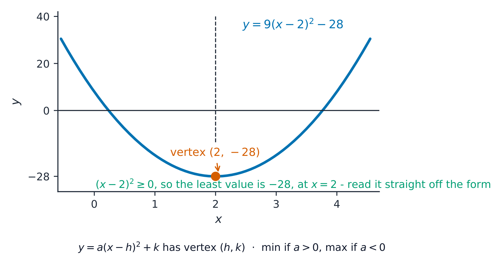
This form is useful: it shows the vertex 顶点 (turning point) of the curve at $(-p,\ q)$, and it gives a quick way to solve the equation.
Worked example. Write $9x^2 - 36x + 8$ in the form $p(x + q)^2 + r$.
Take the factor $9$ out of the first two terms, then complete the square inside:
Factorise: $(k - 4)(k - 16) > 0$, so $k < 4$ or $k > 16$. You also need $a \neq 0$, so $k \neq 0$.
Quadratic equations and inequalities
To solve a quadratic equation 二次方程, factorise, complete the square, or use the formula
$$x = \frac{-b \pm \sqrt{b^2 - 4ac}}{2a}.$$
To solve a quadratic inequality 二次不等式 such as $(k - 4)(k - 16) > 0$, find the two roots, then decide which side of each root makes the statement true. A sketch of the parabola 抛物线 helps: the curve is above the $x$-axis (positive) outside the roots and below it (negative) between them.
Simultaneous equations
To solve a pair of simultaneous equations 联立方程 where one is linear and one is quadratic, use substitution 代入: rearrange the linear equation for one letter, then put that into the quadratic. This gives a single quadratic to solve.
Equations that are quadratic in disguise
Some equations are quadratic in some function of$x$. For example $x^4 - 5x^2 + 4 = 0$ is quadratic in $x^2$: let $u = x^2$, solve $u^2 - 5u + 4 = 0$, then go back to $x$. You will use this idea again in trigonometry.
The shape of a quadratic · รูปร่างของฟังก์ชันกำลังสอง
y = ax² + bx + c
Drag a, b and c. Watch the vertex, the line of symmetry and the roots (where it cuts the x-axis) move as the coefficients change. · ลาก a, b และ c ดู จุดยอด, เส้นสมมาตร และ ราก (จุดตัดแกน x) เคลื่อนที่เมื่อสัมประสิทธิ์เปลี่ยน
understand the terms function, domain, range, one-one function, inverse function and composition of functions
identify the range of a given function in simple cases, and find the composition of two given functions
e.g. range of $f : x \mapsto \frac{1}{x}$ for $x \geqslant 1$ and range of $g : x \mapsto x^2 + 1$ for $x \in \mathbb{R}$. Including the condition that a composite function $gf$ can only be formed when the range of $f$ is within the domain of $g$.
determine whether or not a given function is one-one, and find the inverse of a one-one function in simple cases
e.g. finding the inverse of $h : x \mapsto (2x + 3)^2 - 4$ for $x < -\frac{3}{2}$.
illustrate in graphical terms the relation between a one-one function and its inverse
Sketches should include an indication of the mirror line $y = x$.
understand and use the transformations of the graph of $y = f(x)$ given by $y = f(x) + a$, $y = f(x + a)$, $y = af(x)$, $y = f(ax)$ and simple combinations of these.
Including use of the terms ‘translation’, ‘reflection’ and ‘stretch’ in describing transformations. Questions may involve algebraic or trigonometric functions, or other graphs with given features.
Source: Cambridge International syllabus · แหล่งที่มา: หลักสูตร Cambridge International
English
Transforming graphs: shift and stretch
A function 函数 is a rule that sends each input to exactly one output. Write it as $f(x)$. The composition of functions 复合函数$fg(x)$ means apply $g$ first, then apply $f$ to the result.
The domain 定义域 is the set of allowed inputs $x$.
The range 值域 is the set of outputs the function actually produces.
A function is one-one 一一对应 if different inputs always give different outputs. (No output is repeated.) Only a one-one function has an inverse function 反函数$f^{-1}$, which reverses the rule.
The composition 复合 of two functions means doing one after the other. $fg(x)$ means "do $g$ first, then $f$": $fg(x) = f(g(x))$. The composite function $fg$ exists only when the range of $g$ lies inside the domain of $f$.
Finding an inverse
To find $f^{-1}$: write $y = f(x)$, make $x$ the subject, then swap letters.
Worked example. The function $f(x) = (x + 3)^2 - 12$ is defined for $x \geqslant 0$. Find $f^{-1}(x)$.
Write $y = (x + 3)^2 - 12$ and solve for $x$:
$$(x + 3)^2 = y + 12 \;\Rightarrow\; x + 3 = \sqrt{y + 12} \;\Rightarrow\; x = \sqrt{y + 12} - 3.$$
You take the positive square root because $x \geqslant 0$ means $x + 3 \geqslant 3 > 0$. So
$$f^{-1}(x) = \sqrt{x + 12} - 3.$$
Graphs of inverses and transformations
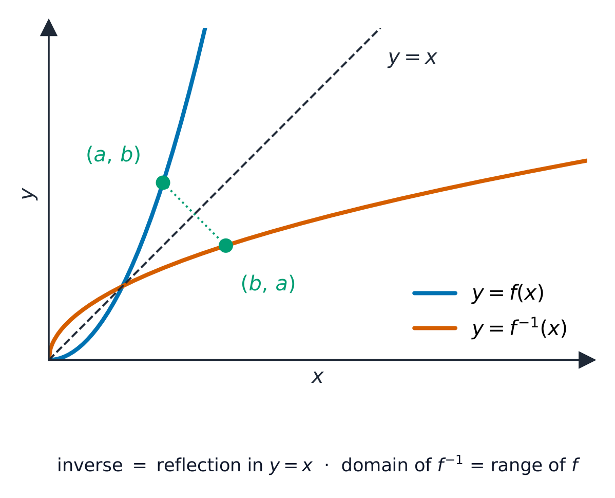
The graph of $y = f^{-1}(x)$ is the reflection 反射 of $y = f(x)$ in the line $y = x$.
You should know these transformations 变换 of $y = f(x)$:
New equation
Effect on the graph
$y = f(x) + a$
translation 平移 up by $a$
$y = f(x + a)$
translation left by $a$
$y = a\,f(x)$
stretch 伸缩 in the $y$-direction, scale factor $a$
$y = f(ax)$
stretch in the $x$-direction, scale factor $\tfrac{1}{a}$
When two transformations are combined, the order can matter. State each one fully (type, direction, and amount).
A function turns each input into exactly one output — drag the coefficients and watch where the curve rises and falls. · ฟังก์ชันแปลง อินพุต แต่ละค่าให้เป็น เอาต์พุต Exactly หนึ่งค่า — ลากสัมประสิทธิ์และดูว่ากราฟ ขึ้น และ ลง ที่ไหน
find the equation of a straight line given sufficient information
e.g. given two points, or one point and the gradient.
interpret and use any of the forms $y = mx + c$, $y - y_1 = m(x - x_1)$, $ax + by + c = 0$ in solving problems
Including calculations of distances, gradients, midpoints, points of intersection and use of the relationship between the gradients of parallel and perpendicular lines.
understand that the equation $(x - a)^2 + (y - b)^2 = r^2$ represents the circle with centre $(a, b)$ and radius $r$
Including use of the expanded form $x^2 + y^2 + 2gx + 2fy + c = 0$.
use algebraic methods to solve problems involving lines and circles
Including use of elementary geometrical properties of circles, e.g. tangent perpendicular to radius, angle in a semicircle, symmetry. Implicit differentiation is not included.
understand the relationship between a graph and its associated algebraic equation, and use the relationship between points of intersection of graphs and solutions of equations.
e.g. to determine the set of values of $k$ for which the line $y = x + k$ intersects, touches or does not meet a quadratic curve.
Source: Cambridge International syllabus · แหล่งที่มา: หลักสูตร Cambridge International
English
What is a radian?
Radians
A radian 弧度 is another way to measure angles. One radian is the angle at the centre of a circle that cuts off an arc 弧 equal in length to the radius. The link between radians and degrees 度 is
$$\pi \text{ radians} = 180^\circ.$$
So to change degrees to radians, multiply by $\dfrac{\pi}{180}$; to change radians to degrees, multiply by $\dfrac{180}{\pi}$.
Arc length and sector area
For a sector 扇形 with radius $r$ and angle $\theta$in radians:
$$\text{arc length} = s = r\theta, \qquad \text{sector area} = A = \tfrac12 r^2 \theta.$$
A chord 弦 cuts the sector into a triangle and a segment 弓形. The segment area is the sector minus the triangle:
Worked example. A sector has centre $O$ and the angle at $O$ is $\tfrac{2}{3}\pi$ radians. Show that the segment cut off by the chord has area about $0.614 r^2$.
Radians, arcs and sectors · เรเดียน, ความยาวส่วนโค้ง และพื้นที่ส่วนวงกลม
Change the angle (in radians) and radius. See the arc length$s = r\theta$ and the sector area$\tfrac12 r^2\theta$ update. · เปลี่ยนมุม (เป็นเรเดียน) และรัศมี ดู ความยาวส่วนโค้ง$s = r\theta$ และ พื้นที่ส่วนวงกลม$\tfrac12 r^2\theta$ อัปเดต
Source: Cambridge International syllabus · แหล่งที่มา: หลักสูตร Cambridge International
English
Amplitude, period and midline of a sine curveThe unit circle draws the sine curve
Graphs and exact values
You must know the shape of the graphs of the sine 正弦, cosine 余弦 and tangent function 正切 (written $\sin$, $\cos$, $\tan$). The sine and cosine graphs wave between $-1$ and $1$ and repeat every $360^\circ$ ($2\pi$). Learn these exact values:
$\theta$
$30^\circ$
$45^\circ$
$60^\circ$
$\sin\theta$
$\tfrac12$
$\tfrac{1}{\sqrt2}$
$\tfrac{\sqrt3}{2}$
$\cos\theta$
$\tfrac{\sqrt3}{2}$
$\tfrac{1}{\sqrt2}$
$\tfrac12$
$\tan\theta$
$\tfrac{1}{\sqrt3}$
$1$
$\sqrt3$
The notations $\sin^{-1}x$, $\cos^{-1}x$, $\tan^{-1}x$ mean the inverse angle (the principal value 主值).
Identities
An identity 恒等式 is true for every value of the angle. The two you must know are
Drag the amplitude, period and shifts of y = a·sin(bx + c) + d and watch the curve change against the base wave. · ลาก Amplitude, Period และการเลื่อนของ y = a·sin(bx + c) + d และดูกราฟเปลี่ยนแปลงเทียบกับคลื่นพื้นฐาน
Explore · สำรวจ
Sine and cosine on the unit circle · ไซน์และโคไซน์บนวงกลมหน่วย
Drag the angle round the unit circle. The height is $\sin\theta$, the across-distance is $\cos\theta$ — that's where the graphs come from. · ลากมุมรอบ วงกลมหน่วย ความสูงคือ $\sin\theta$ ระยะทางแนวนอนคือ $\cos\theta$ — นั่นคือที่มาของกราฟ
use the expansion of $(a + b)^n$, where $n$ is a positive integer
Including the notations $\begin{pmatrix} n \\ r \end{pmatrix}$ and $n!$ Knowledge of the greatest term and properties of the coefficients are not required.
recognise arithmetic and geometric progressions
use the formulae for the $n$th term and for the sum of the first $n$ terms to solve problems involving arithmetic or geometric progressions
Including knowledge that numbers $a$, $b$, $c$ are 'in arithmetic progression' if $2b = a + c$ (or equivalent) and are 'in geometric progression' if $b^2 = ac$ (or equivalent). Questions may involve more than one progression.
use the condition for the convergence of a geometric progression, and the formula for the sum to infinity of a convergent geometric progression.
A progression 数列 (sequence) is a list of terms following a rule.
An arithmetic progression 等差数列 (AP) adds a fixed common difference 公差$d$ each step. The $n$th term 项 is $u_n = a + (n - 1)d$, and the sum of the first $n$ terms is $S_n = \tfrac{n}{2}\big(2a + (n - 1)d\big)$.
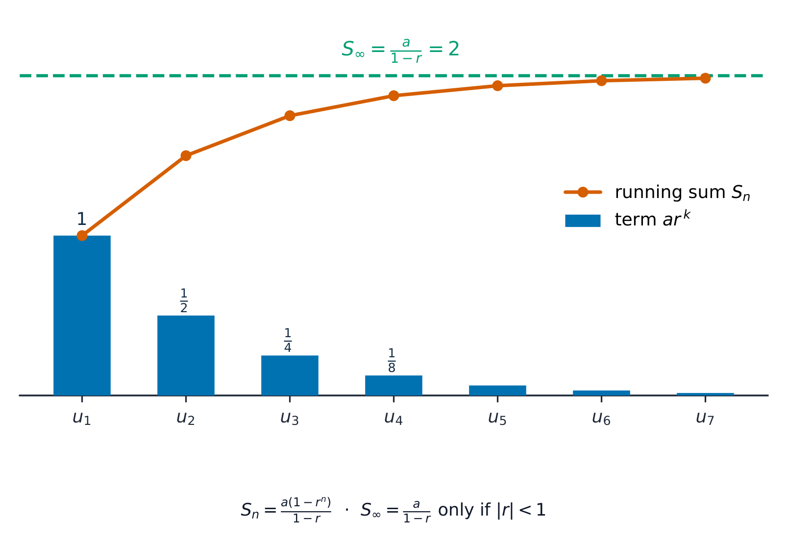
A geometric progression 等比数列 (GP) multiplies by a fixed common ratio 公比$r$ each step. The $n$th term is $u_n = ar^{\,n-1}$, and $S_n = \dfrac{a(1 - r^n)}{1 - r}$.
A GP is convergent — it converges 收敛 (settles to a limit) — when $|r| < 1$. Then it has a sum to infinity 无穷和
$$S_\infty = \frac{a}{1 - r}.$$
Worked example. The third term of a GP is $18$ and the sum of the first three terms is $26$. The common ratio is negative. Find the sum to infinity.
From $ar^2 = 18$ you get $a = \dfrac{18}{r^2}$. Put this into $a(1 + r + r^2) = 26$:
Convergent GP: เสาหดตัวเข้าหาศูนย์ mientras ผลรวมสะสมเข้าใกล้ S infinity = a/(1-r)
Explore · สำรวจ
Arithmetic and geometric sequences · อนุกรมเลขคณิตและเรขาคณิต
Switch between an arithmetic (add d) and a geometric (multiply by r) sequence and watch the terms and their sum build up. · สลับระหว่าง อนุกรมเลขคณิต (บวก d) และ อนุกรมเรขาคณิต (คูณ r) แล้วดูพจน์และผลรวมสะสมเพิ่มขึ้น
understand the gradient of a curve at a point as the limit of the gradients of a suitable sequence of chords, and use the notations $f'(x)$, $f''(x)$, $\frac{\text{d}y}{\text{d}x}$, and $\frac{\text{d}^2y}{\text{d}x^2}$ for first and second derivatives
Only an informal understanding of the idea of a limit is expected. e.g. includes consideration of the gradient of the chord joining the points with $x$ coordinates $2$ and $(2 + h)$ on the curve $y = x^3$. Formal use of the general method of differentiation from first principles is not required.
use the derivative of $x^n$ (for any rational $n$), together with constant multiples, sums and differences of functions, and of composite functions using the chain rule
e.g. find $\frac{\text{d}y}{\text{d}x}$, given $y = \sqrt{2x^3 + 5}$.
apply differentiation to gradients, tangents and normals, increasing and decreasing functions and rates of change
Including connected rates of change, e.g. given the rate of increase of the radius of a circle, find the rate of increase of the area for a specific value of one of the variables.
locate stationary points and determine their nature, and use information about stationary points in sketching graphs.
Including use of the second derivative for identifying maxima and minima; alternatives may be used in questions where no method is specified. Knowledge of points of inflexion is not included.
Source: Cambridge International syllabus · แหล่งที่มา: หลักสูตร Cambridge International
English
Differentiation from first principles
Differentiation 微分 finds the gradient of a curve 曲线斜率 at each point. The gradient is the limit 极限 of the gradients of shorter and shorter chords, called the derivative 导数.
The rules
Write the derivative as $f'(x)$ or $\dfrac{dy}{dx}$. The basic rule is
$$\frac{d}{dx}\left(x^n\right) = n x^{n-1} \quad \text{for any rational } n.$$
Differentiate sums term by term, and use the chain rule 链式法则 for a function inside a function:
$$\frac{d}{dx}\,f(g(x)) = f'(g(x)) \cdot g'(x).$$
Differentiating again gives the second derivative 二阶导数$f''(x)$ or $\dfrac{d^2y}{dx^2}$.
Using the derivative
Tangent and normal. The gradient of the curve at a point is the gradient of the tangent there. The normal 法线 is perpendicular to the tangent, so its gradient is $-\dfrac{1}{\text{(tangent gradient)}}$.
Increasing or decreasing. The function is an increasing function 增函数 where $\dfrac{dy}{dx} > 0$, and a decreasing function 减函数 where $\dfrac{dy}{dx} < 0$.
Rate of change. A derivative is a rate of change 变化率. Linked rates use the chain rule, e.g. $\dfrac{dy}{dt} = \dfrac{dy}{dx}\cdot\dfrac{dx}{dt}$.
Stationary points
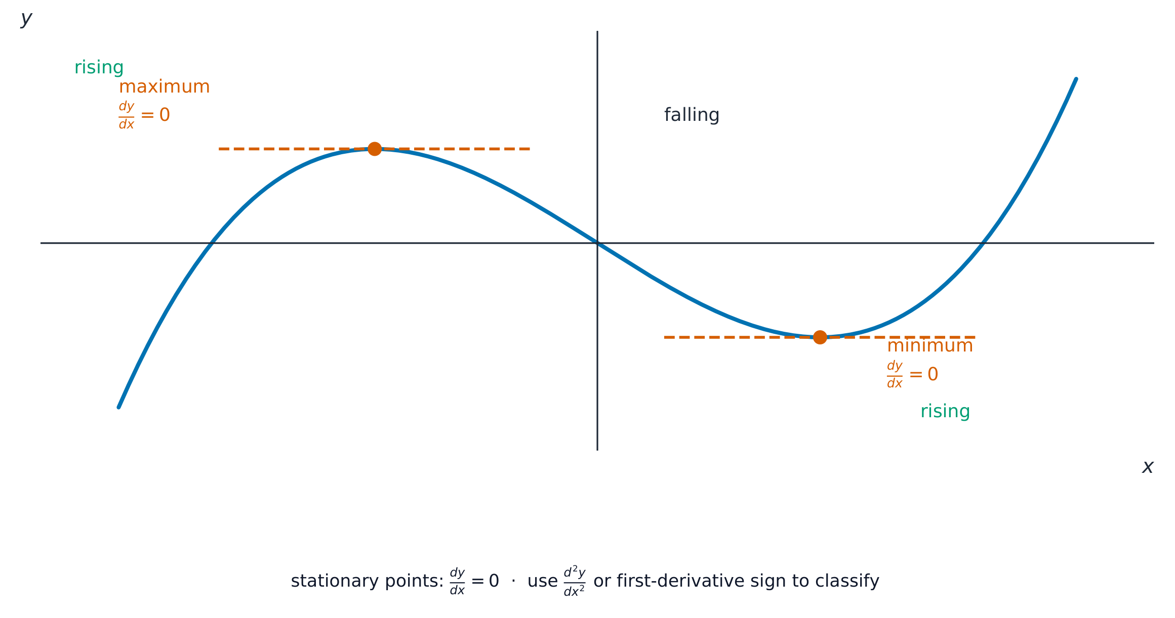
A stationary point 驻点 is where $\dfrac{dy}{dx} = 0$. Test its nature with the second derivative: $f''(x) > 0$ gives a minimum point 极小值点, and $f''(x) < 0$ gives a maximum point 极大值点. When $f''(x) = 0$ the test is inconclusive: the point may be a point of inflexion 拐点, where the curve changes concavity (the way it bends) – check the sign of $\dfrac{dy}{dx}$ just before and after to decide.
Worked example. The curve $y = 4x^{1/2} - x$ has a maximum point at $x = a$. Find $a$.
Slide the point along the curve. The tangent shows the gradient $\frac{dy}{dx}$ there — steeper where the curve bends more. · เลื่อนจุดตามเส้นโค้ง เส้นสัมผัส แสดงความชัน $\frac{dy}{dx}$ ที่จุดนั้น — ชันขึ้นเมื่อเส้นโค้งงอมากขึ้น
equation of a straight line/ɪˈkweɪʒn əvə streɪt laɪn/
สมการเส้นตรง
parallel/ˈpærəlel/
并联电路中
perpendicular/ˌpɜːpənˈdɪkjʊlə/
ตั้งฉาก
chord/kɔːd/
คอร์ด
Differentiation/ˌdɪfəˌrenʃɪˈeɪʃn/
การหาอนุพันธ์
gradient of a curve/ˈɡreɪdɪənt əvə kɜːv/
ความชันของเส้นโค้ง
limit/ˈlɪmɪt/
limit
derivative/dɪˈrɪvətɪv/
อนุพันธ์เชิงซ้อน (ดีริวทีฟ)
chain rule/tʃeɪn ruːl/
กฎโซ่ (Chain Rule)
second derivative/ˈsekənd dɪˈrɪvətɪv/
อนุพันธ์อันดับสอง
normal/ˈnɔːml/
เส้นปกติ
increasing function/ɪnˈkriːsɪŋ ˈfʌŋkʃn/
ฟังก์ชันเพิ่มขึ้น
decreasing function/ˈdiːkriːsɪŋ ˈfʌŋkʃn/
ฟังก์ชันลดลง
rate of change/reɪt ɒv tʃeɪndʒ/
อัตราการเปลี่ยนแปลง
stationary point/ˈsteɪʃənəri pɔɪnt/
จุดนิ่ง
minimum point/ˈmɪnɪməm pɔɪnt/
จุดต่ำสุด
maximum point/ˈmæksɪməm pɔɪnt/
จุดสูงสุด
point of inflexion/pɔɪnt ɒv ɪnˈflekʃn/
จุดเปลี่ยนเว้า
1.8
Integration · การหาอินทิกรัล (Integration)
Syllabus · หลักสูตร
English
Candidates should be able to:
Notes and examples
understand integration as the reverse process of differentiation, and integrate $(ax + b)^n$ (for any rational $n$ except $-1$), together with constant multiples, sums and differences
solve problems involving the evaluation of a constant of integration
e.g. to find the equation of the curve through $(1, -2)$ for which $\frac{\text{d}y}{\text{d}x} = \sqrt{2x + 1}$.
evaluate definite integrals
Including simple cases of 'improper' integrals, such as $\int_{0}^{1} x^{-\frac{1}{2}} \text{d}x$ and $\int_{1}^{\infty} x^{-2} \text{d}x$.
use definite integration to find: - the area of a region bounded by a curve and lines parallel to the axes, or between a curve and a line or between two curves - a volume of revolution about one of the axes.
A volume of revolution may involve a region not bounded by the axis of rotation, e.g. the region between $y = 9 - x^2$ and $y = 5$ rotated about the $x$-axis.
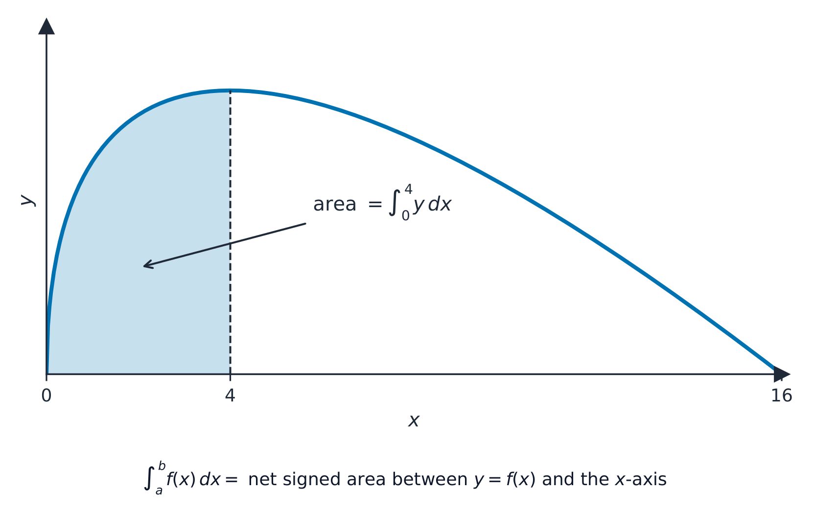
The area of the region 区域 between a curve and the $x$-axis, from $x = p$ to $x = q$, is $\displaystyle\int_p^q y \, dx$. For the area between two curves, integrate (top curve $-$ bottom curve).
Worked example. The curve $y = 4x^{1/2} - x$ meets the $x$-axis again at $x = 16$. Find the area between the curve and the $x$-axis from $x = 0$ to $x = 4$.
and $\displaystyle\int_0^{1}x^{-1/2}\, dx=\left[2x^{1/2}\right]_0^{1}=2$, which is finite even though the integrand blows up at $x=0$.
Volume of revolution
When a region is turned all the way around an axis it sweeps out a solid. The volume of revolution 旋转体体积 about the $x$-axis is
$$V = \pi \int_p^q y^2 \, dx,$$
and about the $y$-axis it is $V = \pi \displaystyle\int x^2 \, dy$. For example, the region under $y = \sqrt{x}$ from $x = 0$ to $x = 4$, turned about the $x$-axis, has volume $\pi\displaystyle\int_0^4 x\, dx = \pi\big[\tfrac{x^2}{2}\big]_0^4 = 8\pi$.
ไทย
Integration ในแง่ของพื้นที่: Riemann rectangles
Integration คือการย้อนกลับของการหาอนุพันธ์ การย้อนกลับ power rule จะได้
Drag the limits. The definite integral is the shaded area between the curve and the x-axis. · ลากขอบเขต อินทิกรัลจำกัด คือพื้นที่แรเงาระหว่างเส้นโค้งกับแกน x
This handout covers Topic 2: Pure Mathematics 纯数学 2. It adds the modulus and polynomial algebra, logarithms 对数 and the exponential function 指数函数, more trigonometry, and new ways to differentiate and integrate.
understand the meaning of $|x|$, sketch the graph of $y = |ax + b|$ and use relations such as $|a| = |b| \iff a^2 = b^2$ and $|x - a| < b \iff a - b < x < a + b$ when solving equations and inequalities
Graphs of $y = |f(x)|$ and $y = f(|x|)$ for non-linear functions $f$ are not included. e.g. $|3x - 2| = |2x + 7|$, $2x + 5 < |x + 1|$
divide a polynomial, of degree not exceeding 4, by a linear or quadratic polynomial, and identify the quotient and remainder (which may be zero)
use the factor theorem and the remainder theorem.
e.g. to find factors and remainders, solve polynomial equations or evaluate unknown coefficients. Including factors of the form $(ax + b)$ in which the coefficient of $x$ is not unity, and including calculation of remainders.
ไทย
ผู้เข้าสอบควรสามารถ:
หมายเหตุและตัวอย่าง
เข้าใจความหมายของ $|x|$, วาดกราฟของ $y = |ax + b|$ และใช้ความสัมพันธ์เช่น $|a| = |b| \iff a^2 = b^2$ และ $|x - a| < b \iff a - b < x < a + b$ เมื่อแก้สมการและอสมการ
Source: Cambridge International syllabus · แหล่งที่มา: หลักสูตร Cambridge International
English
The modulus
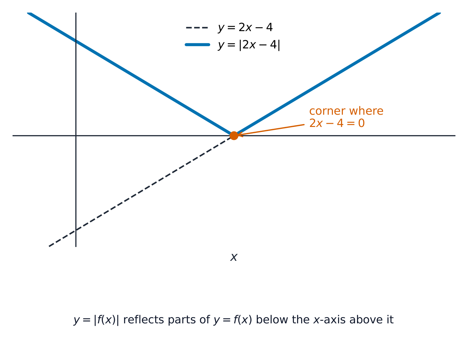
The modulus 绝对值$|x|$ is the size of a number with its sign removed, so $|x| \geqslant 0$ always. The graph of $y = |ax + b|$ is a "V" shape that bounces off the $x$-axis. Two useful rules for solving equations and inequalities are
$$|a| = |b| \;\Leftrightarrow\; a^2 = b^2, \qquad |x - a| < b \;\Leftrightarrow\; a - b < x < a + b.$$
Worked example. Solve $|3x + 8| < 9$.
Using the second rule with the inequality written as $-9 < 3x + 8 < 9$:
Polynomial division and the factor and remainder theorems
A polynomial 多项式 is a sum of powers of $x$, such as $2x^4 + 3x^2 - 5$. Its degree 次数 is the highest power. When you divide one polynomial by another you get a quotient 商 and a remainder 余数.
Remainder theorem 余数定理: the remainder when $p(x)$ is divided by $(x - a)$ is $p(a)$.
Factor theorem 因式定理: $(x - a)$ is a factor of $p(x)$ exactly when $p(a) = 0$.
Worked example. The polynomial $p(x) = 2x^4 + kx^3 + kx^2 + 17x + 18$ has factor $(x + 2)$. Find $k$.
The modulus makes a V-shape. Move its vertex with b and c; change how steep the arms are with a. · ฟังก์ชันค่าสัมบูรณ์ทำให้เกิดรูป ตัว V เลื่อน จุดยอด ด้วย b และ c; เปลี่ยนความชันของ แขน ด้วย a
use logarithms to transform a given relationship to linear form, and hence determine unknown constants by considering the gradient and/or intercept.
e.g. $y = kx^n$ gives $\ln y = \ln k + n \ln x$ which is linear in $\ln x$ and $\ln y$$y = k(a^x)$ gives $\ln y = \ln k + x \ln a$ which is linear in $x$ and $\ln y$.
เช่น $y = kx^n$ ให้ $\ln y = \ln k + n \ln x$ ซึ่งเป็นเชิงเส้นใน $\ln x$ และ $\ln y$$y = k(a^x)$ ให้ $\ln y = \ln k + x \ln a$ ซึ่งเป็นเชิงเส้นใน $x$ และ $\ln y$.
Source: Cambridge International syllabus · แหล่งที่มา: หลักสูตร Cambridge International
English
A logarithm answers the question "what power?". If $a^x = y$ then $x = \log_a y$. Logarithms and indices 指数 (powers) are reverse ideas. The laws of logarithms 对数定律 are
$$\log(mn) = \log m + \log n, \qquad \log\!\frac{m}{n} = \log m - \log n, \qquad \log(m^k) = k\log m.$$
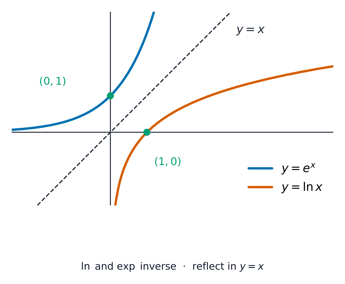
The exponential function $e^x$ and the natural logarithm 自然对数$\ln x$ are inverse functions, so $\ln(e^x) = x$ and $e^{\ln x} = x$. When the unknown is in the power, take logs of both sides.
Linear form 线性形式: a relationship like $y = Ax^n$ becomes a straight line if you take logs: $\ln y = \ln A + n\ln x$. Plotting $\ln y$ against $\ln x$ gives a line with gradient $n$ and intercept $\ln A$, so you can find the unknown constants.
Change the base b: when b > 1 the curve grows, when 0 < b < 1 it decays — and it always passes through (0, a). · เปลี่ยน ฐาน b: เมื่อ b > 1 เส้นโค้งจะ เติบโต, เมื่อ 0 < b < 1 จะ ลดลง — และมันจะผ่านจุด (0, a) เสมอ
understand the relationship of the secant, cosecant and cotangent functions to cosine, sine and tangent, and use properties and graphs of all six trigonometric functions for angles of any magnitude
use trigonometrical identities for the simplification and exact evaluation of expressions, and in the course of solving equations, and select an identity or identities appropriate to the context, showing familiarity in particular with the use of: – $\sec^2 \theta \equiv 1 + \tan^2 \theta$ and $\csc^2 \theta \equiv 1 + \cot^2 \theta$ – the expansions of $\sin(A \pm B)$, $\cos(A \pm B)$ and $\tan(A \pm B)$ – the formulae for $\sin 2A$, $\cos 2A$ and $\tan 2A$ – the expression of $a \sin \theta + b \cos \theta$ in the forms $R \sin(\theta \pm \alpha)$ and $R \cos(\theta \pm \alpha)$.
Source: Cambridge International syllabus · แหล่งที่มา: หลักสูตร Cambridge International
English
There are three more functions, each the reciprocal of one you know: the secant 正割$\sec\theta = \dfrac{1}{\cos\theta}$, the cosecant 余割$\csc\theta = \dfrac{1}{\sin\theta}$, and the cotangent 余切$\cot\theta = \dfrac{1}{\tan\theta}$.
You must know these trigonometric identities 三角恒等式 and choose the right one for each problem:
So $\sec\theta = \tfrac52$ or $\sec\theta = -4$, giving $\cos\theta = \tfrac25$ or $\cos\theta = -\tfrac14$. The solutions are $\theta = \pm 66.4^\circ$ and $\theta = \pm 104.5^\circ$.
Drag the angle to see how $\sin$, $\cos$ and $\tan$ relate — the key to solving trig equations. · ลากมุมเพื่อดูความสัมพันธ์ระหว่าง $\sin$, $\cos$ และ $\tan$ — กุญแจสำคัญในการแก้สมการตรีโกณมิติ
เช่น $x = t - e^{2t}$, $y = t + e^{2t}$. เช่น $x^2 + y^2 = xy + 7$. รวมถึงการใช้ในโจทย์ที่เกี่ยวข้องกับเส้นสัมผัสและเส้นปกติ
Source: Cambridge International syllabus · แหล่งที่มา: หลักสูตร Cambridge International
English
Learn these standard derivatives:
$$\frac{d}{dx}e^x = e^x, \quad \frac{d}{dx}\ln x = \frac{1}{x}, \quad \frac{d}{dx}\sin x = \cos x, \quad \frac{d}{dx}\cos x = -\sin x, \quad \frac{d}{dx}\tan x = \sec^2 x.$$
For a product or a quotient of two functions, use:
the product rule 乘积法则: $(uv)' = u'v + uv'$;
the quotient rule 商法则: $\left(\dfrac{u}{v}\right)' = \dfrac{u'v - uv'}{v^2}$.
When a curve is given by parametric equations 参数方程$x = x(t)$, $y = y(t)$, the gradient is $\dfrac{dy}{dx} = \dfrac{dy/dt}{dx/dt}$. When $y$ is defined implicitly 隐式 (not made the subject), differentiate every term with respect to $x$, using the chain rule on the $y$ terms, then solve for $\dfrac{dy}{dx}$.
Worked example. Given $y = 6x\cos(x^2 + 1)$, find $\dfrac{dy}{dx}$.
Use the product rule with $u = 6x$ and $v = \cos(x^2 + 1)$ (and the chain rule for $v$):
Move the point: the tangent line is the derivative at that x. Where the curve turns, the gradient is zero. · เคลื่อนจุด: เส้นสัมผัส คืออนุพันธ์ที่ค่า x นั้น เมื่อเส้นโค้งเปลี่ยนทิศทาง ความชันจะเป็นศูนย์
• extend the idea of ‘reverse differentiation’ to include the integration of $e^{ax + b}$, $\frac{1}{ax + b}$, $\sin(ax + b)$, $\cos(ax + b)$ and $\sec^2(ax + b)$
Knowledge of the general method of integration by substitution is not required.
• use trigonometrical relationships in carrying out integration
e.g. use of double-angle formulae to integrate $\sin^2 x$ or $\cos^2(2x)$.
• understand and use the trapezium rule to estimate the value of a definite integral.
Including use of sketch graphs in simple cases to determine whether the trapezium rule gives an over-estimate or an under-estimate.
Source: Cambridge International syllabus · แหล่งที่มา: หลักสูตร Cambridge International
English
Integration is reverse differentiation — reverse each new derivative; harder integrals may need integration by substitution 换元积分 (developed in Pure 3). For a linear inside function $(ax + b)$:
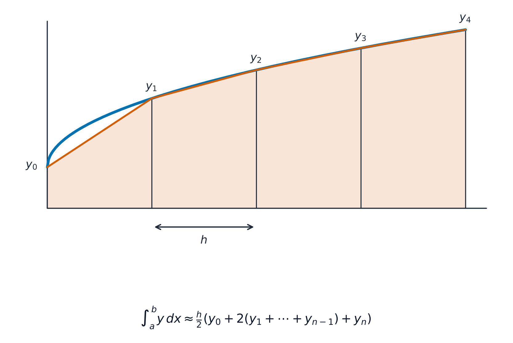
To integrate a power of $\sin$ or $\cos$, first use an identity to remove the power. When you cannot integrate exactly, the trapezium rule 梯形法则 estimates a definite integral:
integration by substitution/ˌɪntɪˈɡreɪʃn baɪ ˌsʌbstɪˈtjuːʃn/
การอินทิเกรตด้วยการแทนตัวแปร
2.6
Numerical solution of equations · การแก้สมการด้วยวิธีเชิงตัวเลข
Syllabus · หลักสูตร
English
Candidates should be able to:
Notes and examples
• locate approximately a root of an equation, by means of graphical considerations and/or searching for a sign change
e.g. finding a pair of consecutive integers between which a root lies.
• understand the idea of, and use the notation for, a sequence of approximations which converges to a root of an equation
• understand how a given simple iterative formula of the form $x_{n + 1} = \text{F}(x_n)$ relates to the equation being solved, and use a given iteration, or an iteration based on a given rearrangement of an equation, to determine a root to a prescribed degree of accuracy.
Knowledge of the condition for convergence is not included, but an understanding that an iteration may fail to converge is expected.
Source: Cambridge International syllabus · แหล่งที่มา: หลักสูตร Cambridge International
English
Iterating to a root: ride the tangent
Many equations cannot be solved exactly. Two ideas help you find a root 根 (a solution).
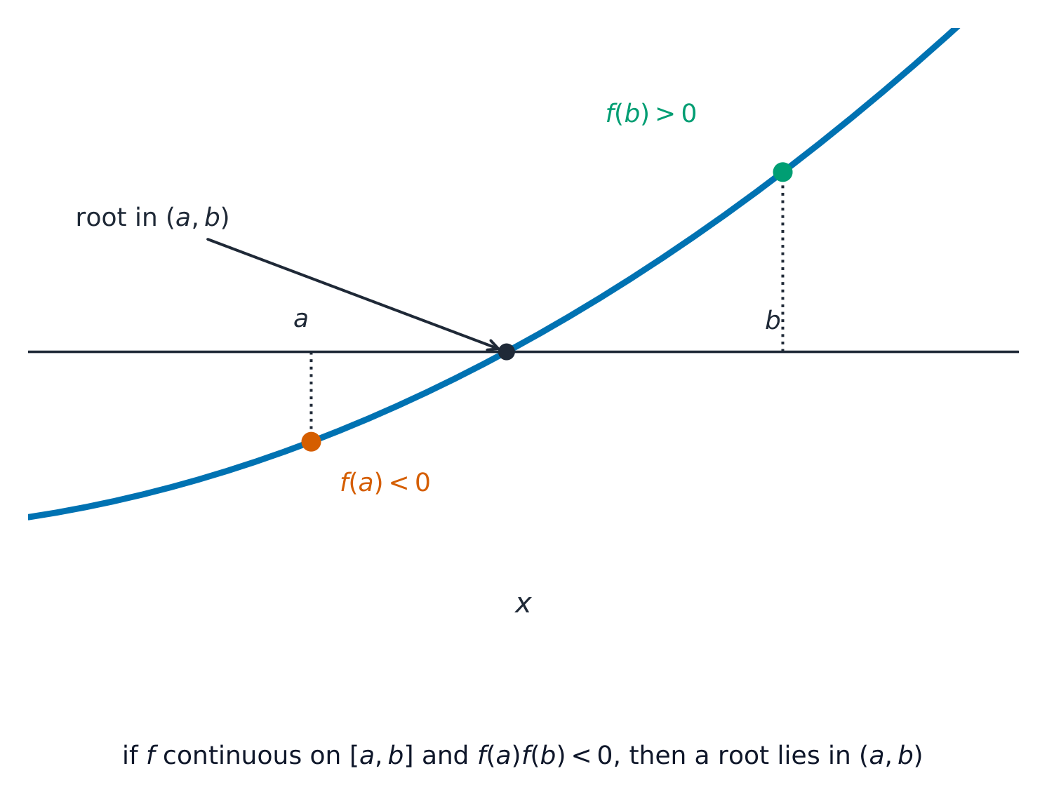
Sign change 变号: if $f(a)$ and $f(b)$ have opposite signs (and the graph has no break between them), a root lies between $a$ and $b$.
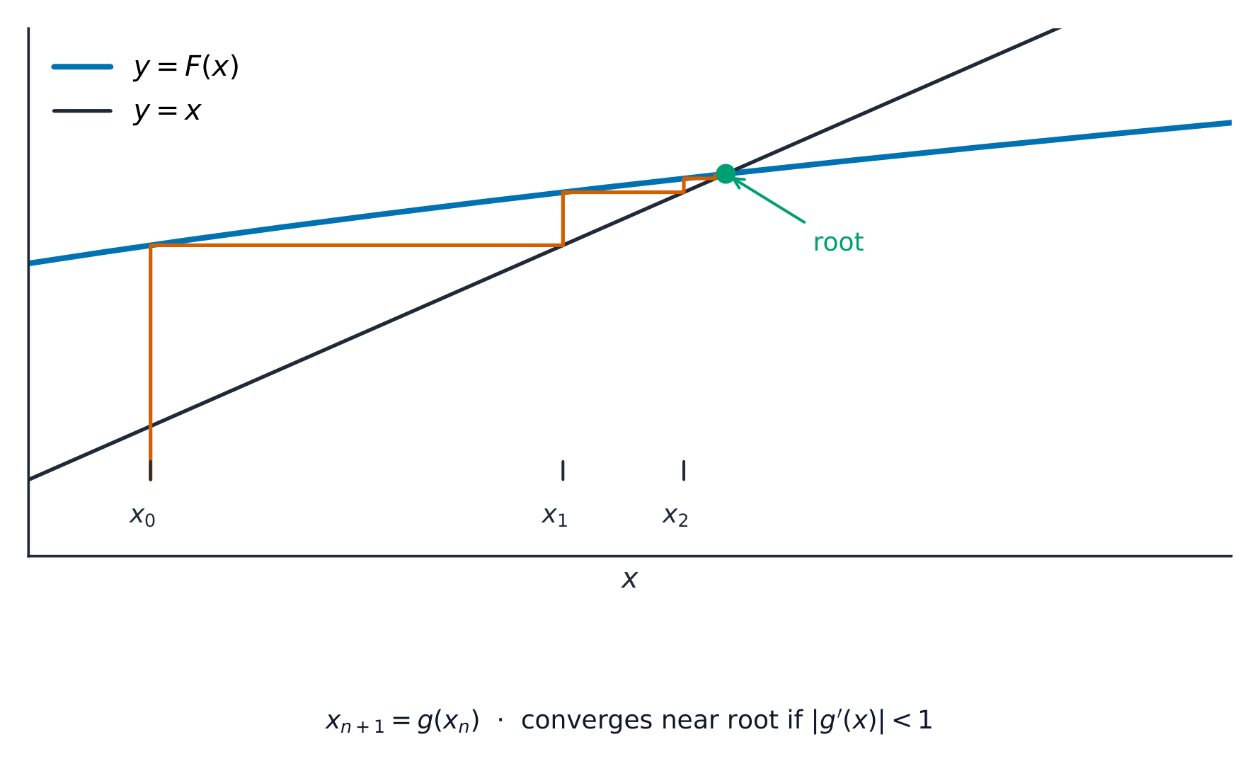
Iteration 迭代: rearrange the equation into the form $x = F(x)$, then use the iterative formula 迭代公式$x_{n+1} = F(x_n)$. Start from a first guess $x_0$ and repeat. If the values are convergent they settle down and converge 收敛 to a root. Keep going until the answer is steady to the accuracy asked for.
Worked example. A root $\beta$ of an equation satisfies $x = \sqrt[3]{-2x - 4.5}$, and $-1.4 < \beta < -1.0$. Use the iteration $x_{n+1} = \sqrt[3]{-2x_n - 4.5}$ with $x_0 = -1.2$.
A root is where the curve crosses zero. A sign change in f(x) traps a root between two x-values. · ราก คือจุดที่กราฟตัดแกนศูนย์ การเปลี่ยนเครื่องหมาย ของ f(x) บ่งบอกว่ามีรากอยู่ระหว่างค่า x สองค่า
This handout covers Topic 3: Pure Mathematics 纯数学 3. Subtopics 3.1–3.6 build on the algebra, logarithms, trigonometry, differentiation, integration and numerical methods of Pure Mathematics 2, so this handout explains what is new in Pure 3 and then covers the three big new areas: vectors, differential equations and complex numbers.
3.1
Algebra
Syllabus · หลักสูตร
English
Candidates should be able to:
Notes and examples
• understand the meaning of $|x|$, sketch the graph of $y = |ax + b|$ and use relations such as $|a| = |b| \iff a^2 = b^2$ and $|x - a| < b \iff a - b < x < a + b$ when solving equations and inequalities
Graphs of $y = |\text{f}(x)|$ and $y = \text{f}(|x|)$ for non-linear functions $\text{f}$ are not included. e.g. $|3x - 2| = |2x + 7|$, $2x + 5 < |x + 1|$.
• divide a polynomial, of degree not exceeding 4, by a linear or quadratic polynomial, and identify the quotient and remainder (which may be zero)
• use the factor theorem and the remainder theorem
e.g. to find factors and remainders, solve polynomial equations or evaluate unknown coefficients. Including factors of the form $(ax + b)$ in which the coefficient of $x$ is not unity, and including calculation of remainders.
• recall an appropriate form for expressing rational functions in partial fractions, and carry out the decomposition, in cases where the denominator is no more complicated than – $(ax + b)(cx + d)(ex + f)$ – $(ax + b)(cx + d)^2$ – $(ax + b)(cx^2 + d)$
Excluding cases where the degree of the numerator exceeds that of the denominator
• use the expansion of $(1 + x)^n$, where $n$ is a rational number and $|x| < 1$.
Finding the general term in an expansion is not included. Adapting the standard series to expand e.g. $(2 - \frac{1}{2}x)^{-1}$ is included, and determining the set of values of $x$ for which the expansion is valid in such cases is also included.
ไทย
ผู้เข้าสอบควรสามารถ:
หมายเหตุและตัวอย่าง
• เข้าใจความหมายของ $|x|$, วาดกราฟของ $y = |ax + b|$ และใช้ความสัมพันธ์เช่น $|a| = |b| \iff a^2 = b^2$ และ $|x - a| < b \iff a - b < x < a + b$ ในการแก้สมการและอสมการ
Source: Cambridge International syllabus · แหล่งที่มา: หลักสูตร Cambridge International
Two new tools join the algebra from Pure 2.
Partial fractions
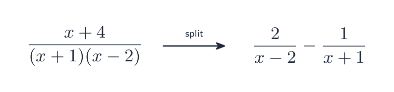
A single fraction with a factorised bottom can be split into a sum of simpler fractions. This is called writing it in partial fractions 部分分式, and it makes a rational function 有理函数 (a fraction of polynomials) easy to integrate or expand. Match the form to the bottom:
First check the top is lower degree than the bottom. If it is not ("top-heavy"), divide the polynomial first: dividing gives a quotient 商 plus a remainder 余数 over the original bottom, and you split only that remaining proper fraction.
One fraction with a factorised bottom splits into a sum of simpler fractions.
For example $(1 + x)^{1/2} = 1 + \tfrac12 x - \tfrac18 x^2 + \cdots$ for $|x| < 1$.
Explore · สำรวจ
Reciprocal curves · โค้งผกผัน
y = a/(x − b) + c
Partial fractions split a hard fraction into simple reciprocal pieces — each with a vertical and a horizontal asymptote. · การแยกเศษส่วนย่อยแยกเศษส่วนยากให้เป็นเศษส่วนย่อยแบบ ผกผัน ที่ง่าย — แต่ละส่วนจะมี เส้นกำกับแนวตั้ง และ เส้นกำกับแนวนอน
use logarithms to transform a given relationship to linear form, and hence determine unknown constants by considering the gradient and/or intercept.
e.g. $y = kx^n$ gives $\ln y = \ln k + n \ln x$ which is linear in $\ln x$ and $\ln y$. $y = k(a^x)$ gives $\ln y = \ln k + x \ln a$ which is linear in $x$ and $\ln y$.
เช่น $y = kx^n$ ให้ $\ln y = \ln k + n \ln x$ ซึ่งเป็นเชิงเส้นใน $\ln x$ และ $\ln y$. $y = k(a^x)$ ให้ $\ln y = \ln k + x \ln a$ ซึ่งเป็นเชิงเส้นใน $x$ และ $\ln y$.
English
Candidates should be able to:
Notes and examples
understand the relationship of the secant, cosecant and cotangent functions to cosine, sine and tangent, and use properties and graphs of all six trigonometric functions for angles of any magnitude
use trigonometrical identities for the simplification and exact evaluation of expressions, and in the course of solving equations, and select an identity or identities appropriate to the context, showing familiarity in particular with the use of: – $\sec^2 \theta \equiv 1 + \tan^2 \theta$ and $\cosec^2 \theta \equiv 1 + \cot^2 \theta$ – the expansions of $\sin(A \pm B)$, $\cos(A \pm B)$ and $\tan(A \pm B)$ – the formulae for $\sin 2A$, $\cos 2A$ and $\tan 2A$ – the expression of $a \sin \theta + b \cos \theta$ in the forms $R \sin(\theta \pm \alpha)$ and $R \cos(\theta \pm \alpha)$.
• locate approximately a root of an equation, by means of graphical considerations and/or searching for a sign change
e.g. finding a pair of consecutive integers between which a root lies.
• understand the idea of, and use the notation for, a sequence of approximations which converges to a root of an equation
• understand how a given simple iterative formula of the form $x_{n+1} = \text{F}(x_n)$ relates to the equation being solved, and use a given iteration, or an iteration based on a given rearrangement of an equation, to determine a root to a prescribed degree of accuracy.
Knowledge of the condition for convergence is not included, but an understanding that an iteration may fail to converge is expected.
Source: Cambridge International syllabus · แหล่งที่มา: หลักสูตร Cambridge International
Iterating to a root: ride the tangent
Subtopics 3.2, 3.3 and 3.6 are the same skills you met in Pure 2: the laws of logarithms with $e^x$ and $\ln x$; the identities $\sec^2\theta \equiv 1 + \tan^2\theta$ and $\csc^2\theta \equiv 1 + \cot^2\theta$, the compound- and double-angle formulae, and the $R$-form of $a\sin\theta + b\cos\theta$; and solving an equation numerically by a sign change 变号 and an iterative formula 迭代公式$x_{n+1} = F(x_n)$. Use them exactly as before.
The three new trig functions are the reciprocals 倒数 of the familiar ones: the secant 正割$\sec\theta = \dfrac{1}{\cos\theta}$, the cosecant 余割$\csc\theta = \dfrac{1}{\sin\theta}$, and the cotangent 余切$\cot\theta = \dfrac{1}{\tan\theta} = \dfrac{\cos\theta}{\sin\theta}$. (Memory aid: match the third letter — sec goes with cosine.) The two Pythagorean identities above come straight from dividing $\sin^2\theta + \cos^2\theta \equiv 1$ by $\cos^2\theta$ or $\sin^2\theta$. For a numerical method, an iteration $x_{n+1}=F(x_n)$converges 收敛 to the root when successive values get closer together.
Explore · สำรวจ
The unit circle · วงกลมหน่วย
(cos θ, sin θ)
The R-formula rewrites a sin θ + b cos θ as one wave — and it all lives on this circle. · สูตร R เขียน a sin θ + b cos θ ในรูปคลื่นเดียว — และทั้งหมดอยู่บนวงกลมนี้
เช่น $x = t - e^{2t}$, $y = t + e^{2t}$. เช่น $x^2 + y^2 = xy + 7$. รวมถึงการใช้ในโจทย์ที่เกี่ยวข้องกับเส้นสัมผัสและเส้นปกติ
Source: Cambridge International syllabus · แหล่งที่มา: หลักสูตร Cambridge International
The methods are those of Pure 2 (the product, quotient and chain rules, with parametric and implicit curves). One derivative is added — the inverse tangent 反正切:
$$\frac{d}{dx}\tan^{-1} x = \frac{1}{1 + x^2}.$$
Worked example. Differentiate $y = \tan^{-1}(3x)$.
Use the chain rule with the result above: $\dfrac{dy}{dx} = \dfrac{1}{1 + (3x)^2} \times 3 = \dfrac{3}{1 + 9x^2}.$
Explore · สำรวจ
The gradient at a point · ความชันที่จุดหนึ่ง
gradient = dy/dx
Implicit or not, the derivative is still the slope of the tangent — slide the point to see it. · ไม่ว่าจะเป็นอนุพันธ์แบบชัดแจ้งหรือไม่ ความชันของ เส้นสัมผัส ก็ยังคงเป็น อนุพันธ์ — เลื่อนจุดเพื่อดูได้
extend the idea of 'reverse differentiation' to include the integration of $e^{ax + b}$, $\frac{1}{ax + b}$, $\sin(ax + b)$, $\cos(ax + b)$, $\sec^2(ax + b)$ and $\frac{1}{x^2 + a^2}$
Including examples such as $\frac{1}{2 + 3x^2}$.
use trigonometrical relationships in carrying out integration
e.g. use of double-angle formulae to integrate $\sin^2 x$ or $\cos^2(2x)$.
integrate rational functions by means of decomposition into partial fractions
Restricted to types of partial fractions as specified in topic 3.1 above.
recognise an integrand of the form $\frac{k f'(x)}{f(x)}$, and integrate such functions
e.g. integration of $\frac{x}{x^2 + 1}$, $\tan x$.
recognise when an integrand can usefully be regarded as a product, and use integration by parts
e.g. integration of $x \sin 2x$, $x^2 e^{-x}$, $\ln x$, $x \tan^{-1} x$.
use a given substitution to simplify and evaluate either a definite or an indefinite integral.
e.g. to integrate $\sin^2 2x \cos x$ using the substitution $u = \sin x$.
Source: Cambridge International syllabus · แหล่งที่มา: หลักสูตร Cambridge International
Pure 3 adds several powerful methods.
A new standard integral: $\displaystyle\int \frac{1}{x^2 + a^2}\,dx = \frac{1}{a}\tan^{-1}\frac{x}{a} + C$.
Partial fractions: split a rational function first, then integrate each piece as a logarithm.
The pattern $\dfrac{k\,f'(x)}{f(x)}$: this integrates to $k\ln|f(x)| + C$. For example $\displaystyle\int \frac{2x}{x^2 + 1}\,dx = \ln(x^2 + 1) + C$.
Integration by parts 分部积分, used for a product: $\displaystyle\int u\,\frac{dv}{dx}\,dx = uv - \int v\,\frac{du}{dx}\,dx$.
Integration by substitution 换元积分: a given change of variable turns a hard integral into an easy one.
Worked example. Find $\displaystyle\int x\cos x\,dx$.
Use integration by parts with $u = x$ and $\dfrac{dv}{dx} = \cos x$, so $\dfrac{du}{dx} = 1$ and $v = \sin x$:
$$\int x\cos x\,dx = x\sin x - \int \sin x\,dx = x\sin x + \cos x + C.$$
Explore · สำรวจ
The area under the curve · พื้นที่ใต้กราฟ
area = ∫ f(x) dx
Every integration method just measures this area — drag the limits to total it. · วิธีการอินทิเกรตทั้งหมดวัด พื้นที่ นี้ — ลากขอบเขตเพื่อรวมค่าทั้งหมด
Integration by substitution/ˌɪntɪˈɡreɪʃn baɪ ˌsʌbstɪˈtjuːʃn/
การอินทิเกรตด้วยการแทนที่
3.7
Vectors
Syllabus · หลักสูตร
English
Candidates should be able to:
Notes and examples
• use standard notations for vectors, i.e. $\begin{pmatrix} x \\ y \end{pmatrix}$, $x\mathbf{i} + y\mathbf{j}$, $\begin{pmatrix} x \\ y \\ z \end{pmatrix}$, $x\mathbf{i} + y\mathbf{j} + z\mathbf{k}$, $\overrightarrow{AB}$, $\mathbf{a}$
• carry out addition and subtraction of vectors and multiplication of a vector by a scalar, and interpret these operations in geometrical terms
e.g. ‘$OABC$ is a parallelogram’ is equivalent to $\overrightarrow{OB} = \overrightarrow{OA} + \overrightarrow{OC}$. The general form of the ratio theorem is not included, but understanding that the midpoint of $AB$ has position vector $\frac{1}{2}(\overrightarrow{OA} + \overrightarrow{OB})$ is expected.
• calculate the magnitude of a vector, and use unit vectors, displacement vectors and position vectors
In 2 or 3 dimensions.
• understand the significance of all the symbols used when the equation of a straight line is expressed in the form $\mathbf{r} = \mathbf{a} + t\mathbf{b}$, and find the equation of a line, given sufficient information
e.g. finding the equation of a line given the position vector of a point on the line and a direction vector, or the position vectors of two points on the line.
• determine whether two lines are parallel, intersect or are skew, and find the point of intersection of two lines when it exists
Calculation of the shortest distance between two skew lines is not required. Finding the equation of the common perpendicular to two skew lines is also not required.
• use formulae to calculate the scalar product of two vectors, and use scalar products in problems involving lines and points.
e.g. finding the angle between two lines, and finding the foot of the perpendicular from a point to a line; questions may involve 3D objects such as cuboids, tetrahedra (pyramids), etc. Knowledge of the vector product is not required.
ไทย
ผู้เข้าสอบควรสามารถ:
หมายเหตุและตัวอย่าง
• ใช้สัญลักษณ์มาตรฐานสำหรับ เวกเตอร์ คือ $\begin{pmatrix} x \\ y \end{pmatrix}$, $x\mathbf{i} + y\mathbf{j}$, $\begin{pmatrix} x \\ y \\ z \end{pmatrix}$, $x\mathbf{i} + y\mathbf{j} + z\mathbf{k}$, $\overrightarrow{AB}$, $\mathbf{a}$
Source: Cambridge International syllabus · แหล่งที่มา: หลักสูตร Cambridge International
Forces like wind and water are vectors — they have both size and direction.
A vector 向量 has both size and direction. Write it as a column, or as $x\mathbf{i} + y\mathbf{j} + z\mathbf{k}$, or as $\overrightarrow{AB}$.
The magnitude 模长 (length) of $\mathbf{v} = x\mathbf{i} + y\mathbf{j} + z\mathbf{k}$ is $|\mathbf{v}| = \sqrt{x^2 + y^2 + z^2}$.
A unit vector 单位向量 has magnitude $1$; divide a vector by its magnitude to make one.
A position vector 位置向量 gives a point's place from the origin; a displacement vector 位移向量$\overrightarrow{AB} = \mathbf{b} - \mathbf{a}$ goes from one point to another. Multiplying by a scalar 标量 (a plain number) stretches a vector.
Lines and the scalar product
A straight line through point $\mathbf{a}$ in direction $\mathbf{b}$ has vector equation $\mathbf{r} = \mathbf{a} + t\mathbf{b}$. Two lines may be parallel 平行, may intersect 相交 at a point, or may be skew lines 异面直线 (not parallel and never meeting).
Start at the point $\mathbf{a}$, then add $t$ copies of the direction $\mathbf{b}$ to reach any point on the line.
The scalar product 数量积 (dot product) of $\mathbf{a}$ and $\mathbf{b}$ is
where $\theta$ is the angle between them. So $\mathbf{a}\cdot\mathbf{b} = 0$ means the vectors are perpendicular.
The scalar product picks out $|\mathbf{b}|\cos\theta$, how far $\mathbf{b}$ reaches along $\mathbf{a}$.
Worked example. Find the angle between $\mathbf{a} = \mathbf{i} + 2\mathbf{j} + 2\mathbf{k}$ and $\mathbf{b} = 2\mathbf{i} + 2\mathbf{j} + \mathbf{k}$.
Adding vectors and the dot product · การบวกเวกเตอร์และผลคูณสเกลาร์
Drag the two vectors. See the resultant (tip-to-tail) and the dot product, which is zero when they are perpendicular. · ลากเวกเตอร์สองตัว ดู เวกเตอร์ผลรวม (ปลายติดต้น) และ ผลคูณสเกลาร์ ซึ่งเป็นศูนย์เมื่อตั้งฉากกัน
Source: Cambridge International syllabus · แหล่งที่มา: หลักสูตร Cambridge International
A differential equation 微分方程 links a quantity to its rate of change. To solve a first-order equation whose variables are separable 可分离变量, put all the $y$ terms on one side and all the $x$ terms on the other, then integrate both sides. This gives the general solution 通解, which contains a constant. An initial condition 初始条件 (a known value) fixes the constant and gives the particular solution 特解.
Worked example. Solve $\dfrac{dy}{dx} = xy$, given that $y = 1$ when $x = 0$.
Separate the variables and integrate:
$$\int \frac{1}{y}\,dy = \int x\,dx \;\Rightarrow\; \ln y = \tfrac12 x^2 + c \;\Rightarrow\; y = A e^{x^2/2}.$$
Using $y = 1$ at $x = 0$ gives $A = 1$, so $y = e^{x^2/2}$.
The constant $A$ gives a whole family of curves; the condition $y=1$ at $x=0$ selects $y=e^{x^2/2}$.
Explore · สำรวจ
A slope field · สนามความชัน
Each little line shows the gradient $\frac{dy}{dx}$ there. A solution curve follows the arrows — change the starting point to see a different one. · เส้นเล็กๆ แต่ละเส้นแสดงความชัน $\frac{dy}{dx}$ ที่จุดนั้น เส้นโซลูชัน ตามลูกศร — เปลี่ยนจุดเริ่มต้นเพื่อดูเส้นอื่น
understand the idea of a complex number, recall the meaning of the terms real part, imaginary part, modulus, argument, conjugate, and use the fact that two complex numbers are equal if and only if both real and imaginary parts are equal
Notations $\text{Re } z$, $\text{Im } z$, $|z|$, $\arg z$, $z^*$ should be known. The argument of a complex number will usually refer to an angle $\theta$ such that $-\pi < \theta \leqslant \pi$, but in some cases the interval $0 \leqslant \theta < 2\pi$ may be more convenient. Answers may use either interval unless the question specifies otherwise.
carry out operations of addition, subtraction, multiplication and division of two complex numbers expressed in Cartesian form$x + \text{i}y$
For calculations involving multiplication or division, full details of the working should be shown.
use the result that, for a polynomial equation with real coefficients, any non-real roots occur in conjugate pairs
e.g. in solving a cubic or quartic equation where one complex root is given.
represent complex numbers geometrically by means of an Argand diagram
carry out operations of multiplication and division of two complex numbers expressed in polar form$r(\cos \theta + \text{i}\sin \theta) \equiv r\text{e}^{\text{i}\theta}$
Including the results $|z_1 z_2| = |z_1||z_2|$ and $\arg(z_1 z_2) = \arg(z_1) + \arg(z_2)$, and corresponding results for division.
find the two square roots of a complex number
e.g. the square roots of $5 + 12\text{i}$ in exact Cartesian form. Full details of the working should be shown.
understand in simple terms the geometrical effects of conjugating a complex number and of adding, subtracting, multiplying and dividing two complex numbers
illustrate simple equations and inequalities involving complex numbers by means of loci in an Argand diagram
e.g. $|z - a| < k$, $|z - a| = |z - b|$, $\arg(z - a) = \alpha$.
Source: Cambridge International syllabus · แหล่งที่มา: หลักสูตร Cambridge International
Multiplying complex numbers: lengths multiply, angles addMultiplying by i is a rotationSelf-similar patterns like Romanesco arise from iterating functions in the complex plane.
A complex number 复数 has the form $z = x + iy$, where $i^2 = -1$. Here $x$ is the real part 实部 and $y$ is the imaginary part 虚部. This $x + iy$ is the Cartesian form 直角坐标形式. Two complex numbers are equal only when their real parts match and their imaginary parts match.
The conjugate 共轭 of $z = x + iy$ is $z^* = x - iy$. For a polynomial with real coefficients, any non-real roots come in conjugate pairs.
The modulus 模 is $|z| = \sqrt{x^2 + y^2}$ (its distance from the origin) and the argument 辐角 is the angle the point makes, measured from the positive real axis.
You can plot $z$ as a point on an Argand diagram 阿干图 (the complex plane).
The polar form 极坐标形式 is $z = r(\cos\theta + i\sin\theta) = re^{i\theta}$, where $r = |z|$ and $\theta$ is the argument. Multiplying multiplies the moduli and adds the arguments.
The loci of points satisfying a condition on $z$ are drawn on the Argand diagram — e.g. $|z - a| = r$ is a circle, $|z - a| = |z - b|$ a perpendicular bisector, and $\arg(z - a) = \theta$ a half-line. The square roots of a complex number come from solving $w^2 = z$.
On the Argand diagram $|z|$ is the distance from $O$, $\arg z$ the angle, and $z^{*}$ the reflection in the real axis.
To divide, multiply top and bottom by the conjugate of the bottom.
Worked example. Write $\dfrac{3 + i}{1 - i}$ in the form $x + iy$.
An equation or inequality in $z$ describes a locus 轨迹 (a path or region) on the Argand diagram. For example $|z - a| = r$ is a circle of radius $r$ centred at $a$.
$|z-a|=r$ is the set of points a fixed distance $r$ from $a$ — a circle.
Explore · สำรวจ
The Argand diagram
Drag the point. A complex number $a + bi$ is a point on the plane; its modulus is the distance from the origin and its argument is the angle. · ลากจุด จำนวนเชิงซ้อน $a + bi$ เป็นจุดบนระนาบ; โมดูลัส คือระยะจากจุดกำเนิด และ อาร์กิวเมนต์ คือมุม
This handout covers Topic 4: Mechanics 力学. It studies how forces make objects move. Throughout this topic, take the acceleration of free fall as $g = 10\ \text{m s}^{-2}$.
understand the vector nature of force, and find and use components and resultants
Calculations are always required, not approximate solutions by scale drawing.
use the principle that, when a particle is in equilibrium, the vector sum of the forces acting is zero, or equivalently, that the sum of the components in any direction is zero
Solutions by resolving are usually expected, but equivalent methods (e.g. triangle of forces, Lami's Theorem, where suitable) are also acceptable; these other methods are not required knowledge, and will not be referred to in questions.
understand that a contact force between two surfaces can be represented by two components, the normal component and the frictional component
use the model of a 'smooth' contact, and understand the limitations of this model
understand the concepts of limiting friction and limiting equilibrium, recall the definition of coefficient of friction, and use the relationship $F = \mu R$ or $F \leqslant \mu R$, as appropriate
Terminology such as 'about to slip' may be used to mean 'in limiting equilibrium' in questions.
use Newton's third law.
e.g. the force exerted by a particle on the ground is equal and opposite to the force exerted by the ground on the particle.
Source: Cambridge International syllabus · แหล่งที่มา: หลักสูตร Cambridge International
English
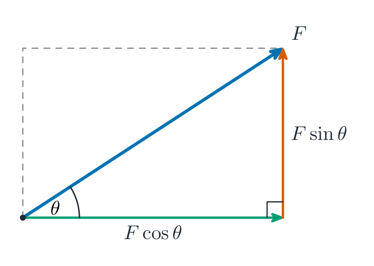
A force 力 is a push or a pull. It is a vector, so it has size and direction. Because it is a vector, you can split a force into components 分量 (usually horizontal and vertical), and you can add several forces into one resultant 合力.
A particle is in equilibrium 平衡 when the forces are balanced: the vector sum of the forces is zero. In practice this means the components in any direction add to zero.
Friction
When two surfaces touch, the contact force 接触力 between them has two parts: the normal reaction 法向反作用力$R$, at right angles to the surface, and the friction 摩擦力$F$, along the surface, which opposes sliding. A "smooth" surface is a model with no friction.
Friction can only grow up to a maximum. At that maximum the body is in limiting equilibrium 极限平衡, about to slip, and the friction is limiting friction 最大静摩擦力. The maximum is set by the coefficient of friction 摩擦系数$\mu$:
$$F \leqslant \mu R, \qquad \text{with } F = \mu R \text{ at the point of slipping}.$$
By Newton's third law 牛顿第三定律, the two surfaces push on each other with equal and opposite forces.
Worked example. A block of weight $20\text{ N}$ rests on a rough horizontal table with coefficient of friction $\mu = 0.4$. Find the largest horizontal force that can be applied before the block slides.
The table's normal reaction balances the weight, so $R = 20\text{ N}$. The block is on the point of slipping when friction reaches its maximum $F = \mu R = 0.4 \times 20 = 8\text{ N}$. In equilibrium the applied force equals the friction, so the largest force it can resist is $8\text{ N}$.
Kinematics of motion in a straight line · จลนวิทยาของการเคลื่อนที่ในเส้นตรง
Syllabus · หลักสูตร
English
Candidates should be able to:
Notes and examples
understand the concepts of distance and speed as scalar quantities, and of displacement, velocity and acceleration as vector quantities
Restricted to motion in one dimension only. The term 'deceleration' may sometimes be used in the context of decreasing speed.
sketch and interpret displacement–time graphs and velocity–time graphs, and in particular appreciate that – the area under a velocity–time graph represents displacement, – the gradient of a displacement–time graph represents velocity, – the gradient of a velocity–time graph represents acceleration
use differentiation and integration with respect to time to solve simple problems concerning displacement, velocity and acceleration
Calculus required is restricted to techniques from the content for Paper 1: Pure Mathematics 1.
use appropriate formulae for motion with constant acceleration in a straight line.
Questions may involve setting up more than one equation, using information about the motion of different particles.
Source: Cambridge International syllabus · แหล่งที่มา: หลักสูตร Cambridge International
English
Distance 距离 and speed 速率 are scalars (size only). Displacement 位移, velocity 速度 and acceleration 加速度 are vectors (size and direction).
On a velocity-time graph 速度时间图, the area under the graph is the displacement and the gradient is the acceleration (a negative acceleration is a deceleration 减速度). On a displacement-time graph, the gradient is the velocity. More generally, differentiate with respect to time to go from displacement to velocity to acceleration, and integrate to go back.
For motion with constant acceleration 匀加速, use these formulae (the "suvat" equations):
$$v = u + at, \qquad s = ut + \tfrac12 at^2, \qquad v^2 = u^2 + 2as, \qquad s = \tfrac12(u + v)t.$$
Worked example. A car starts from rest and accelerates at $2.5\ \text{m s}^{-2}$ for $4\ \text{s}$. Find its speed and the distance travelled.
Change the start velocity and acceleration. The gradient is the acceleration; the area under the line is the displacement. · เปลี่ยนความเร็วเริ่มต้นและความเร่ง ความชัน คือความเร่ง; พื้นที่ใต้เส้นคือระยะกระจัด
Source: Cambridge International syllabus · แหล่งที่มา: หลักสูตร Cambridge International
English
The linear momentum 动量 of a body is $\text{mass} \times \text{velocity}$. It is a vector. In a direct collision of two bodies, the total momentum is unchanged. This is the conservation of linear momentum 动量守恒:
$$m_1 u_1 + m_2 u_2 = m_1 v_1 + m_2 v_2.$$
Worked example. A body of mass $2\ \text{kg}$ moving at $3\ \text{m s}^{-1}$ hits a stationary body of mass $1\ \text{kg}$, and they stick together. Find their common speed afterwards.
Set each mass and speed and collide them. Total momentum stays the same before and after. · ตั้งมวลและความเร็วของแต่ละวัตถุแล้วชนกัน โมเมนตัมรวมคงที่ ก่อนและหลังการชน
conservation of momentum/ˌkɒnsəˈveɪʃn ɒv məʊˈmentəm/
การอนุรักษ์โมเมนตัม
Newton's laws of motion/ˈnjuːtnz lɔːz ɒv ˈməʊʃn/
กฎการเคลื่อนที่ของนิวตัน
mass/mæs/
มวล
weight/weɪt/
น้ำหนัก
tension/ˈtenʃn/
แรงตึง
4.4
Newton's laws of motion · กฎการเคลื่อนที่ของนิวตัน
Syllabus · หลักสูตร
English
Candidates should be able to:
Notes and examples
• apply Newton’s laws of motion to the linear motion of a particle of constant mass moving under the action of constant forces, which may include friction, tension in an inextensible string and thrust in a connecting rod
If any other forces resisting motion are to be considered (e.g. air resistance) this will be indicated in the question.
• use the relationship between mass and weight
$W = mg$. In this component, questions are mainly numerical, and use of the approximate numerical value $10\text{ (ms}^{-2}\text{)}$ for $g$ is expected.
• solve simple problems which may be modelled as the motion of a particle moving vertically or on an inclined plane with constant acceleration
Including, for example, motion of a particle on a rough plane where the acceleration while moving up the plane is different from the acceleration while moving down the plane.
• solve simple problems which may be modelled as the motion of connected particles.
e.g. particles connected by a light inextensible string passing over a smooth pulley, or a car towing a trailer by means of either a light rope or a light rigid tow-bar.
Source: Cambridge International syllabus · แหล่งที่มา: หลักสูตร Cambridge International
English
Newton's laws of motion 牛顿运动定律 connect force and acceleration. The key one is: resultant force $=$mass 质量$\times$ acceleration,
$$F = ma.$$
The weight 重力 of a body is the force of gravity on it: $W = mg$. Forces in a problem may include weight, friction, tension 张力 in a string, the thrust 推力 (push) in a rod, and air resistance 空气阻力.
For motion on an inclined plane 斜面, split each force into a part along the slope and a part at right angles to it, then apply $F = ma$ along the slope. For connected particles 连接质点 (joined by a string), apply $F = ma$ to each body, or to the whole system.
Worked example. A block of mass $12\ \text{kg}$ is pulled up a rough plane by a rope parallel to the slope. The plane is at $20^\circ$ to the horizontal, the coefficient of friction is $0.4$, and the acceleration is $2\ \text{m s}^{-2}$. Find the tension in the rope.
The normal reaction is $R = mg\cos 20^\circ = 120\cos 20^\circ = 112.8\ \text{N}$, so the friction is $F = \mu R = 0.4 \times 112.8 = 45.1\ \text{N}$. Along the slope, $T - mg\sin 20^\circ - F = ma$:
• understand the concept of the work done by a force, and calculate the work done by a constant force when its point of application undergoes a displacement not necessarily parallel to the force
$W = Fd \cos \theta$; Use of the scalar product is not required.
• understand the concepts of gravitational potential energy and kinetic energy, and use appropriate formulae
• understand and use the relationship between the change in energy of a system and the work done by the external forces, and use in appropriate cases the principle of conservation of energy
Including cases where the motion may not be linear (e.g. a child on a smooth curved ‘slide’), where only overall energy changes need to be considered.
• use the definition of power as the rate at which a force does work, and use the relationship between power, force and velocity for a force acting in the direction of motion
Including calculation of (average) power as
$$\frac{\text{Work done}}{\text{Time taken}}$$
$P = Fv$.
• solve problems involving, for example, the instantaneous acceleration of a car moving on a hill against a resistance.
Source: Cambridge International syllabus · แหล่งที่มา: หลักสูตร Cambridge International
English
The work done 功 by a constant force is the scalar product of force and displacement — the force times the distance moved in the direction of the force: $W = Fd\cos\theta$, where $\theta$ is the angle between the force and the motion. Work is measured in joules (J).
Energy comes in forms you can calculate:
Kinetic energy 动能 (energy of movement): $\text{KE} = \tfrac12 mv^2$.
Gravitational potential energy 重力势能 (energy of height): $\text{PE} = mgh$.
The work done by the outside forces equals the change in the total energy. When no friction acts, the total energy stays the same — the conservation of energy 能量守恒.
Power 功率 is the rate of doing work. For a force pulling in the direction of motion, $P = Fv$ (power $=$ force $\times$ velocity). Power is measured in watts (W).
Worked example. A car engine works at $12\ \text{kW}$ while the car moves at $20\ \text{m s}^{-1}$ on a level road. Find the driving force.
งานที่ทำ oleh一个constant force คือ ผลคูณสเกลาร์ of force and displacement — the force times the distance moved in the direction of the force: $W = Fd\cos\theta$, where $\theta$ is the angle between the force and the motion. Work is measured in joules (J).
Energy comes in forms you can calculate:
พลังงานจลน์ (energy of movement): $\text{KE} = \tfrac12 mv^2$.
พลังงานศักย์โน้มถ่วง (energy of height): $\text{PE} = mgh$.
งานที่ทำโดยแรงภายนอกเท่ากับผลต่างของพลังงานทั้งหมด เมื่อไม่มีแรงเสียดทาน พลังงานทั้งหมดจะคงที่ — นี่คือ กฎการอนุรักษ์พลังงาน (conservation of energy).
Drop the object and watch energy change form. With no friction, GPE + KE stays constant the whole way down. · ปล่อยวัตถุแล้วดูการเปลี่ยนแปลงพลังงาน เมื่อไม่มีแรงเสียดทาน GPE + KE คงที่ ตลอดการตก
This handout covers Topic 5: Probability & Statistics 概率统计 1. It is about describing data, counting choices, and working out the chance of events.
5.1
Representation of data
Syllabus · หลักสูตร
English
Candidates should be able to:
Notes and examples
• select a suitable way of presenting raw statistical data, and discuss advantages and/or disadvantages that particular representations may have
• draw and interpret stem-and-leaf diagrams, box-and-whisker plots, histograms and cumulative frequency graphs
Including back-to-back stem-and-leaf diagrams.
• understand and use different measures of central tendency (mean, median, mode) and variation (range, interquartile range, standard deviation)
e.g. in comparing and contrasting sets of data.
• use a cumulative frequency graph
e.g. to estimate medians, quartiles, percentiles, the proportion of a distribution above (or below) a given value, or between two values.
• calculate and use the mean and standard deviation of a set of data (including grouped data) either from the data itself or from given totals $\Sigma x$ and $\Sigma x^2$, or coded totals $\Sigma(x - a)$ and $\Sigma(x - a)^2$, and use such totals in solving problems which may involve up to two data sets.
Source: Cambridge International syllabus · แหล่งที่มา: หลักสูตร Cambridge International
Choose a diagram that suits the data. You should be able to draw and read:
a stem-and-leaf diagram 茎叶图 (keeps the original values and shows the shape); two data sets are compared with a back-to-back 背靠背 version – a shared central stem, one set's leaves increasing to the left and the other's to the right, so you can compare their medians and spreads at a glance;
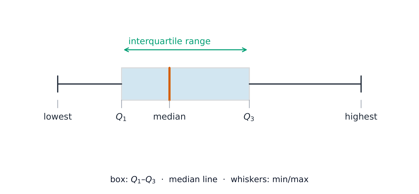
a box-and-whisker plot 箱线图 (shows the lowest value, the three quartiles, and the highest value);
a histogram 直方图 (for grouped data, where the area of each bar shows the frequency);
a cumulative frequency 累积频数 graph (running totals, used to estimate the median and quartiles).
A cumulative frequency curve is S-shaped; read the median across from half the total frequency, and the quartiles from one and three quartersThe box spans the quartiles $Q_1$ to $Q_3$; the whiskers reach the lowest and highest values.
Averages and spread
A measure of central tendency 集中趋势 is a single "middle" value:
the mean 平均数$\bar{x} = \dfrac{\sum x}{n}$ (the average);
the median 中位数 (the middle value when the data is in order);
the mode 众数 (the most common value).
A measure of variation 离散程度 shows how spread out the data is:
the range (of data) 极差 (highest $-$ lowest);
the interquartile range 四分位距 (upper quartile $-$ lower quartile);
the standard deviation 标准差$\sigma = \sqrt{\dfrac{\sum x^2}{n} - \bar{x}^2}$.
You often work from the totals $\sum x$ and $\sum x^2$. The square of the standard deviation is the variance 方差.
Worked example. For $10$ values, $\sum x = 50$ and $\sum x^2 = 300$. Find the mean and standard deviation.
Coding 编码 makes big numbers easier. Replace each value by $t=x-a$ for a convenient assumed mean 假定平均数$a$. Then $\bar{x}=a+\bar{t}$, while the standard deviation is unchanged (shifting every value does not spread the data). So from the coded totals $\sum(x-a)$ and $\sum(x-a)^2$ you get $\bar x$ and $\sigma$ directly, and two data sets can be compared through their coded totals.
Explore · สำรวจ
Spread and the bell · การกระจายและรูปทรงกระดิ่ง
P(−k < Z < k)
Spread is measured in standard deviations — about 68% of data lies within 1 sd, 95% within 2. · การกระจายวัดได้ด้วย ส่วนเบี่ยงเบนมาตรฐาน — ประมาณ 68% ของข้อมูลอยู่ภายใน 1 sd, 95% ภายใน 2
measure of central tendency/ˈmeʒə ɒv ˈsentrəl ˈtendənsi/
ค่ากลาง
mean/miːn/
ค่าเฉลี่ย
median/ˈmiːdiːən/
มัธยฐาน
mode/məʊd/
โมด
variation/ˌveərɪˈeɪʃn/
ความหลากหลาย (Variation)
range (of data)/reɪndʒ/
ช่วง (ของข้อมูล)
interquartile range/ˌɪntəˈkwɔːtaɪl reɪndʒ/
ช่วงระหว่างควอไทล์
standard deviation/ˈstændəd ˌdiːvɪˈeɪʃn/
ส่วนเบี่ยงเบนมาตรฐาน
variance/ˈveərɪəns/
ความแปรปรวน
Coding/ˈkəʊdɪŋ/
Coding
assumed mean/əˈsjuːmd miːn/
ค่าเฉลี่ยสมมติ
central tendency/ˈsentrəl ˈtendənsi/
ค่ากลาง
5.2
Permutations and combinations
Syllabus · หลักสูตร
English
Candidates should be able to:
Notes and examples
• understand the terms permutation and combination, and solve simple problems involving selections
• solve problems about arrangements of objects in a line, including those involving – repetition (e.g. the number of ways of arranging the letters of the word ‘NEEDLESS’) – restriction (e.g. the number of ways several people can stand in a line if two particular people must, or must not, stand next to each other).
Questions may include cases such as people sitting in two (or more) rows. Questions about objects arranged in a circle will not be included.
To arrange objects in a line when some are repeated, divide by the factorial of each repeat count.
Order matters for a permutation, but not for a combination
Worked example. How many different arrangements are there of the letters of the word NEEDLESS?
There are $8$ letters, with E repeated $3$ times and S repeated $2$ times:
evaluate probabilities in simple cases by means of enumeration of equiprobable elementary events, or by calculation using permutations or combinations
e.g. the total score when two fair dice are thrown. e.g. drawing balls at random from a bag containing balls of different colours.
use addition and multiplication of probabilities, as appropriate, in simple cases
Explicit use of the general formula $\text{P}(A \cup B) = \text{P}(A) + \text{P}(B) - \text{P}(A \cap B)$ is not required.
understand the meaning of exclusive and independent events, including determination of whether events $A$ and $B$ are independent by comparing the values of $\text{P}(A \cap B)$ and $\text{P}(A) \times \text{P}(B)$
calculate and use conditional probabilities in simple cases.
e.g. situations that can be represented by a sample space of equiprobable elementary events, or a tree diagram. The use of $\text{P}(A|B) = \frac{\text{P}(A \cap B)}{\text{P}(B)}$ may be required in simple cases.
Source: Cambridge International syllabus · แหล่งที่มา: หลักสูตร Cambridge International
Dice: a familiar starting point for probability.
Find a probability by counting equally likely outcomes, or by using permutations and combinations. Combine probabilities with these rules:
addition for "or": $P(A \cup B) = P(A) + P(B) - P(A \cap B)$;
multiplication for "and" when events are independent: $P(A \cap B) = P(A)\,P(B)$.
The overlap of the two circles is $A\cap B$; the addition rule subtracts it once so it is not counted twice.
Two events are mutually exclusive events 互斥事件 if they cannot both happen, and independent events 独立事件 if one happening does not change the chance of the other. To test independence, check whether $P(A \cap B) = P(A)\times P(B)$. A conditional probability 条件概率 is the chance of $A$ given that $B$ has happened: $P(A \mid B) = \dfrac{P(A \cap B)}{P(B)}$.
Worked example. Events have $P(A) = 0.5$, $P(B) = 0.4$ and $P(A \cap B) = 0.2$. Are $A$ and $B$ independent?
Test: $P(A)\times P(B) = 0.5 \times 0.4 = 0.2 = P(A \cap B)$. The values are equal, so $A$ and $B$ are independent.
Explore · สำรวจ
Conditional probability · ความน่าจะเป็นแบบมีเงื่อนไข
Change the probabilities and read the tree. This is how P(A and B) and conditional probability fit together. · เปลี่ยนความน่าจะเป็นและอ่าน ต้นไม้ วิธีนี้แสดง P(A และ B) และความน่าจะเป็นแบบเงื่อนไขที่เชื่อมโยงกัน
draw up a probability distribution table relating to a given situation involving a discrete random variable$X$, and calculate $\text{E}(X)$ and $\text{Var}(X)$
use formulae for probabilities for the binomial and geometric distributions, and recognise practical situations where these distributions are suitable models
Including the notations $\text{B}(n, p)$ and $\text{Geo}(p)$. $\text{Geo}(p)$ denotes the distribution in which $p_r = p(1 - p)^{r-1}$ for $r = 1, 2, 3, \dots$.
use formulae for the expectation and variance of the binomial distribution and for the expectation of the geometric distribution.
Source: Cambridge International syllabus · แหล่งที่มา: หลักสูตร Cambridge International
A discrete random variable 离散型随机变量$X$ takes separate values, each with a probability. List them in a probability distribution table 概率分布表; the probabilities must add to $1$. Then the expectation 期望 (mean) and variance are
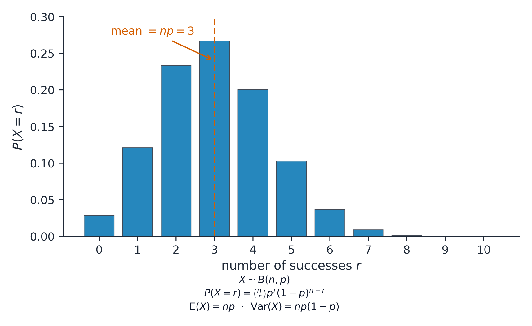
the binomial distribution 二项分布$X \sim B(n, p)$, for the number of successes in $n$ independent trials: $P(X = r) = \binom{n}{r}p^r(1-p)^{n-r}$, with $E(X) = np$ and $\mathrm{Var}(X) = np(1-p)$;
the geometric distribution 几何分布, for the trial on which the first success happens: $P(X = r) = (1-p)^{r-1}p$, with $E(X) = \dfrac{1}{p}$.
Worked example.$X \sim B(10, 0.3)$. Find $P(X = 2)$ and $E(X)$.
The distribution $B(10,0.3)$: each bar is $P(X=r)$, clustered around the mean $np=3$.
Explore · สำรวจ
A discrete distribution · การแจกแจงแบบไม่ต่อเนื่อง
Change n and p for a binomial distribution and watch the bars — the probability of each number of successes. · เปลี่ยน n และ p สำหรับการแจกแจง ทวินาม แล้วดูแท่งกราฟ — ความน่าจะเป็นของจำนวนความสำเร็จแต่ละจำนวน
understand the use of a normal distribution to model a continuous random variable, and use normal distribution tables
Sketches of normal curves to illustrate distributions or probabilities may be required.
solve problems concerning a variable $X$, where $X \sim N(\mu, \sigma^2)$, including: – finding the value of $P(X > x_1)$, or a related probability, given the values of $x_1$, $\mu$, $\sigma$. – finding a relationship between $x_1$, $\mu$ and $\sigma$ given the value of $P(X > x_1)$ or a related probability
For calculations involving standardisation, full details of the working should be shown. e.g. $Z = \frac{(X - \mu)}{\sigma}$
recall conditions under which the normal distribution can be used as an approximation to the binomial distribution, and use this approximation, with a continuity correction, in solving problems.
$n$ sufficiently large to ensure that both $np > 5$ and $nq > 5$.
Source: Cambridge International syllabus · แหล่งที่มา: หลักสูตร Cambridge International
The 68-95-99.7 ruleA Galton board: balls falling through pins pile up into the bell-shaped normal distribution.
The normal distribution 正态分布 models a continuous random variable 连续型随机变量 with a symmetric bell shape. Write $X \sim N(\mu, \sigma^2)$, where $\mu$ is the mean and $\sigma$ is the standard deviation. To use the tables, by standardisation 标准化 convert to the variable $Z \sim N(0, 1)$:
$$Z = \frac{X - \mu}{\sigma}.$$
Then $P(X < x) = P\!\left(Z < \dfrac{x - \mu}{\sigma}\right)$, which you read from the normal table $\Phi$.
A normal probability is an area under the bell curve; standardizing rescales it to $Z\sim N(0,1)$.
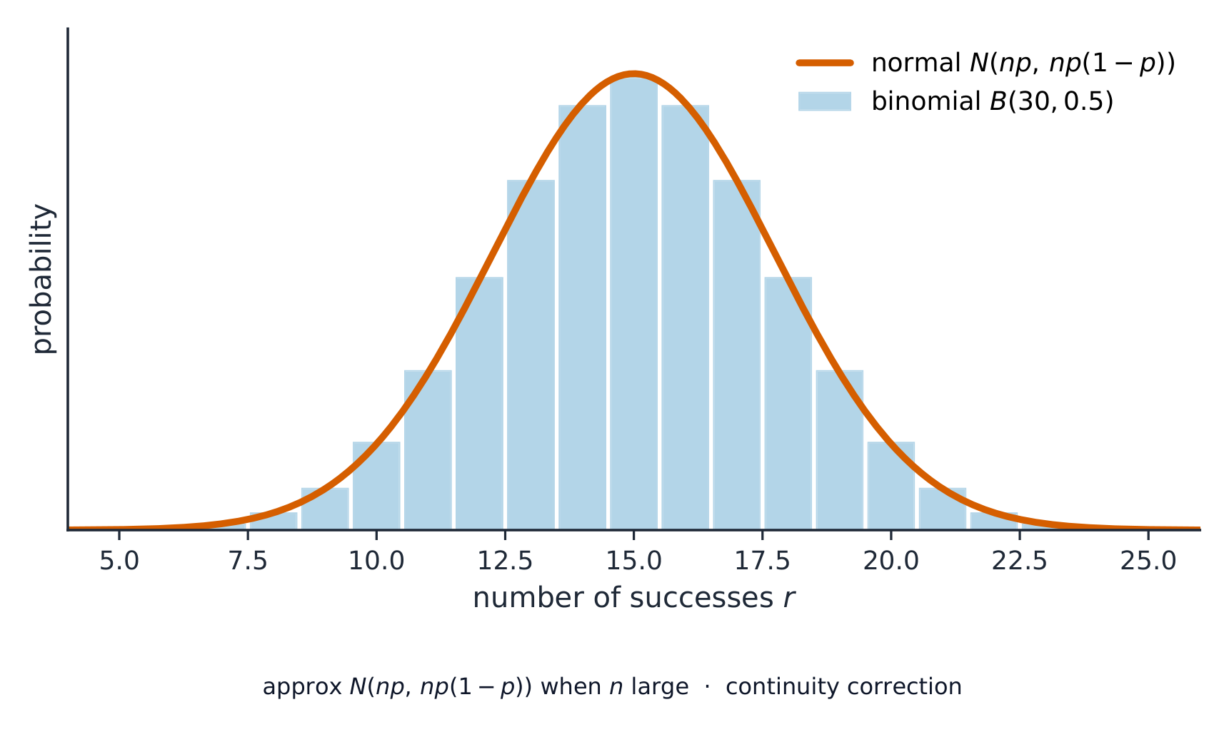
The normal distribution is also a good approximation 近似 to the binomial when $n$ is large. Because you replace a discrete variable by a continuous one, apply a continuity correction 连续性校正 (adjust by $0.5$).
When $n$ is large the binomial bars follow a normal curve of the same mean and variance.
Worked example. Bags of rice have mass $X \sim N(\mu, 0.14^2)$. Given that $P(X < 1.48) = 0.22$, find $\mu$.
From the table, $P(Z < z) = 0.22$ gives $z = -0.772$. So
Shade the area to find a probability. A z-value measures how many standard deviations a point is from the mean. · แรเงาพื้นที่เพื่อหาค่าความน่าจะเป็น ค่า z วัดว่าจุดหนึ่งห่างจากค่าเฉลี่ยกี่เบี่ยงเบนมาตรฐาน
This handout covers Topic 6: Probability & Statistics 概率统计 2. It adds the Poisson model, combining random variables, continuous distributions, and the ideas of estimation and testing.
6.1
The Poisson distribution
Syllabus · หลักสูตร
English
Candidates should be able to:
Notes and examples
• use formulae to calculate probabilities for the distribution $\text{Po}(\lambda)$
• use the fact that if $X \sim \text{Po}(\lambda)$ then the mean and variance of $X$ are each equal to $\lambda$
Proofs are not required.
• understand the relevance of the Poisson distribution to the distribution of random events, and use the Poisson distribution as a model
• use the Poisson distribution as an approximation to the binomial distribution where appropriate
The conditions that $n$ is large and $p$ is small should be known; $n > 50$ and $np < 5$, approximately.
• use the normal distribution, with continuity correction, as an approximation to the Poisson distribution where appropriate.
The condition that $\lambda$ is large should be known; $\lambda > 15$, approximately.
Source: Cambridge International syllabus · แหล่งที่มา: หลักสูตร Cambridge International
People arriving at random in a queue follow a Poisson distribution.
The Poisson distribution 泊松分布$X \sim \mathrm{Po}(\lambda)$ models the number of random events in a fixed interval, when events happen at a steady average rate $\lambda$:
$$P(X = r) = e^{-\lambda}\frac{\lambda^r}{r!}.$$
For a Poisson variable the mean and the variance are both equal to $\lambda$. The Poisson distribution is a good approximation 近似 to the binomial distribution when $n$ is large and $p$ is small. The normal distribution (with continuity correction) approximates the Poisson when $\lambda$ is large.
Worked example.$X \sim \mathrm{Po}(3)$. Find $P(X = 2)$.
The Poisson distribution $\mathrm{Po}(3)$: for a Poisson variable the mean and variance both equal $\lambda$.
Explore · สำรวจ
The Poisson distribution · การแจกแจงปอยซง
Change the mean λ. Poisson models the number of random events in a fixed interval — rare events give a skewed shape. · เปลี่ยนค่าเฉลี่ย λ Poisson ใช้จำลองจำนวน เหตุการณ์สุ่ม ในช่วงเวลาที่กำหนด — เหตุการณ์หายากให้รูปร่างเบ้
• use, when solving problems, the results that – $\text{E}(aX + b) = a\text{E}(X) + b$ and $\text{Var}(aX + b) = a^2\text{Var}(X)$ – $\text{E}(aX + bY) = a\text{E}(X) + b\text{E}(Y)$ – $\text{Var}(aX + bY) = a^2\text{Var}(X) + b^2\text{Var}(Y)$ for independent $X$ and $Y$ – if $X$ has a normal distribution then so does $aX + b$ – if $X$ and $Y$ have independent normal distributions then $aX + bY$ has a normal distribution – if $X$ and $Y$ have independent Poisson distributions then $X + Y$ has a Poisson distribution.
• understand the concept of a continuous random variable, and recall and use properties of a probability density function
For density functions defined over a single interval only; the domain may be infinite, e.g. $\frac{3}{x^4}$ for $x \geqslant 1$.
• use a probability density function to solve problems involving probabilities, and to calculate the mean and variance of a distribution.
Including location of the median or other percentiles of a distribution by direct consideration of an area using the density function. Explicit knowledge of the cumulative distribution function is not included.
Source: Cambridge International syllabus · แหล่งที่มา: หลักสูตร Cambridge International
A continuous random variable 连续型随机变量 can take any value in a range. Its probabilities come from a probability density function 概率密度函数$f(x)$, with two key properties:
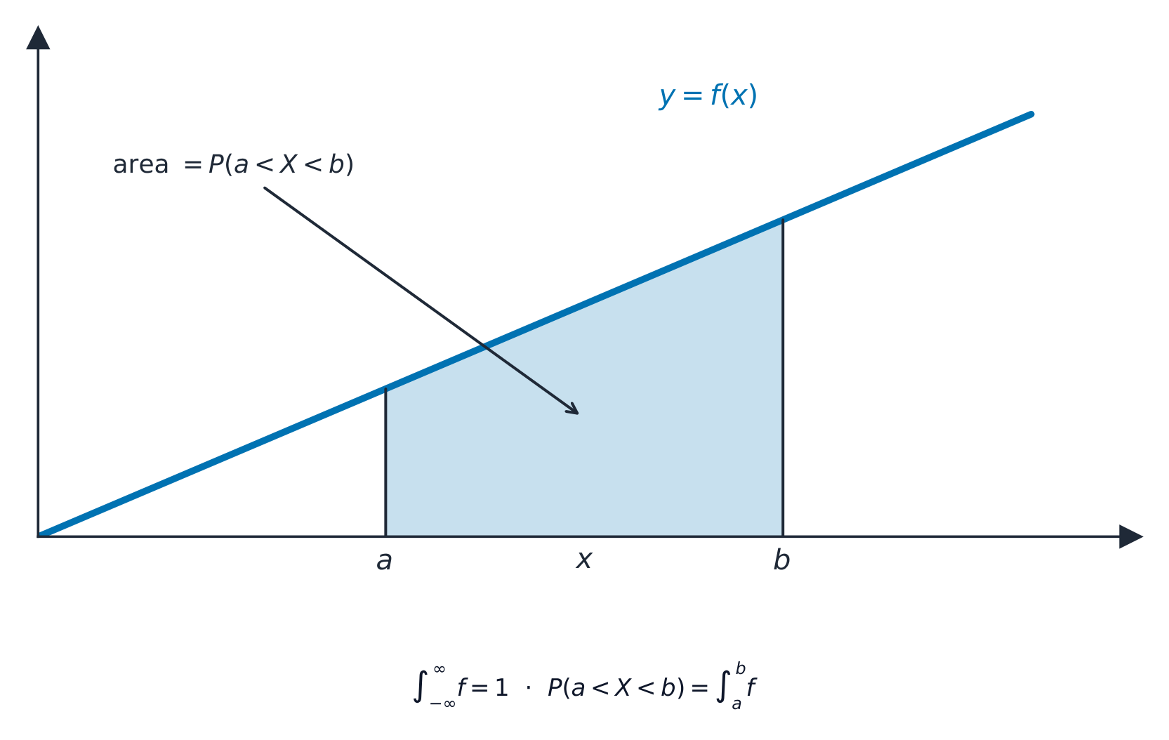
A probability is the area under $f$, and the mean is found by integration:
$$P(a < X < b) = \int_a^b f(x)\,dx, \qquad E(X) = \int_{-\infty}^{\infty} x\,f(x)\,dx.$$
The cumulative distribution function 累积分布函数 is $F(x) = P(X \leqslant x) = \int_{-\infty}^{x} f(t)\,dt$; the median 中位数 solves $F(m) = 0.5$, and other percentiles 百分位数 solve $F(x) = p$.
For a continuous variable, the probability $P(a is the area under $f(x)$ between $a$ and $b$.
Worked example. A continuous variable has $f(x) = \tfrac12 x$ for $0 \leqslant x \leqslant 2$ (and $0$ elsewhere). Find $E(X)$.
The variance uses the same idea, $\mathrm{Var}(X)=\displaystyle\int_{-\infty}^{\infty}x^2 f(x)\,dx-\big(E(X)\big)^2$. For the same $f(x)=\tfrac12 x$ on $[0,2]$: $\displaystyle\int_0^2 x^2\cdot\tfrac12 x\,dx=\left[\tfrac{x^4}{8}\right]_0^2=2$, so $\mathrm{Var}(X)=2-\left(\tfrac43\right)^2=2-\tfrac{16}{9}=\tfrac{2}{9}$.
Explore · สำรวจ
Area = probability · พื้นที่ = ความน่าจะเป็น
P(a < X < b) = ∫ f(x) dx
For a continuous variable, probability is the area under the density curve between two values. · สำหรับตัวแปรต่อเนื่อง ความน่าจะเป็น คือ พื้นที่ใต้เส้นโค้งความหนาแน่นระหว่างสองค่า
• understand the distinction between a sample and a population, and appreciate the necessity for randomness in choosing samples
• explain in simple terms why a given sampling method may be unsatisfactory
Including an elementary understanding of the use of random numbers in producing random samples. Knowledge of particular sampling methods, such as quota or stratified sampling, is not required.
• recognise that a sample mean can be regarded as a random variable, and use the facts that $\text{E}(\overline{X}) = \mu$ and that $\text{Var}(\overline{X}) = \frac{\sigma^2}{n}$
• use the fact that $\overline{X}$ has a normal distribution if $X$ has a normal distribution
• use the Central Limit Theorem where appropriate
Only an informal understanding of the Central Limit Theorem (CLT) is required; for large sample sizes, the distribution of a sample mean is approximately normal.
• calculate unbiased estimates of the population mean and variance from a sample, using either raw or summarised data
Only a simple understanding of the term 'unbiased' is required, e.g. that although individual estimates will vary the process gives an accurate result 'on average'.
• determine and interpret a confidence interval for a population mean in cases where the population is normally distributed with known variance or where a large sample is used
• determine, from a large sample, an approximate confidence interval for a population proportion.
Source: Cambridge International syllabus · แหล่งที่มา: หลักสูตร Cambridge International
Statistics studies a sample to learn about a whole population.
A sample 样本 is a small group chosen from the whole population 总体. A random sample needs randomness 随机性, so that every member has a fair chance of being chosen.
Some methods are unsatisfactory because they are biased 有偏: sampling only volunteers, or the first 20 people to arrive, over-represents certain kinds of people. A genuinely random sample uses random numbers – number every member of the population, then draw numbers (from a table or a generator) to decide who is in the sample.
The sample mean $\bar{X}$ is itself a random variable, with
By the Central Limit Theorem 中心极限定理, for a large sample $\bar{X}$ is approximately normal, whatever the shape of the population.
Whatever the population's shape, the sample mean $\bar{X}$ has a narrow, near-normal distribution centred on $\mu$.
From a sample you can find unbiased estimates 无偏估计 of the population mean and variance. A confidence interval 置信区间 gives a range that probably contains the true mean. When the population is normal with known $\sigma$ (or the sample is large), a $95\%$ interval is
$$\bar{x} \pm 1.96\,\frac{\sigma}{\sqrt{n}}.$$
A $95\%$ confidence interval stretches $1.96$ standard errors each side of the sample mean.
You can also find a confidence interval for a population proportion 总体比例 from a large sample.
Worked example. A sample of $n = 64$ has mean $\bar{x} = 50$, from a population with $\sigma = 8$. Find a $95\%$ confidence interval for the population mean.
The sampling distribution · การแจกแจงของตัวอย่าง
X̄ ~ N(μ, σ²/n)
By the Central Limit Theorem, sample means follow a normal curve — narrower for bigger samples. · โดย ทฤษฎีบทحدกลาง ค่าเฉลี่ยตัวอย่างจะปฏิบัติตามรูปทรง ปกติ — จะแคบลงเมื่อขนาดตัวอย่างใหญ่ขึ้น
• understand the nature of a hypothesis test, the difference between one-tailed and two-tailed tests, and the terms null hypothesis, alternative hypothesis, significance level, rejection region (or critical region), acceptance region and test statistic
Outcomes of hypothesis tests are expected to be interpreted in terms of the contexts in which questions are set.
• formulate hypotheses and carry out a hypothesis test in the context of a single observation from a population which has a binomial or Poisson distribution, using – direct evaluation of probabilities – a normal approximation to the binomial or the Poisson distribution, where appropriate
• formulate hypotheses and carry out a hypothesis test concerning the population mean in cases where the population is normally distributed with known variance or where a large sample is used
• understand the terms Type I error and Type II error in relation to hypothesis tests
• calculate the probabilities of making Type I and Type II errors in specific situations involving tests based on a normal distribution or direct evaluation of binomial or Poisson probabilities.
Source: Cambridge International syllabus · แหล่งที่มา: หลักสูตร Cambridge International
A hypothesis test 假设检验 uses sample data to judge a claim. You set up two statements: the null hypothesis 原假设$H_0$ (the claim being tested, usually "no change") and the alternative hypothesis 备择假设$H_1$ (what you suspect instead). The test is one-tailed 单尾 if $H_1$ points one way (e.g. $\mu > 50$) and two-tailed 双尾 if it allows both ways ($\mu \neq 50$).
You fix a significance level 显著性水平 (often $5\%$), work out a test statistic 检验统计量 from the data, and see whether it lands in the rejection region 拒绝域 (also called the critical region); if it does you reject $H_0$, otherwise the statistic is in the acceptance region.
A two-tailed test at $5\%$ rejects $H_0$ only if the test statistic falls in a shaded tail beyond $\pm1.96$.
Two mistakes are possible: a Type I error 第一类错误 is rejecting $H_0$ when it is actually true; a Type II error 第二类错误 is accepting $H_0$ when it is actually false. You can find their probabilities from the rejection region: $P(\text{Type I})=P(\text{statistic in the rejection region}\mid H_0)$ – this equals the significance level – and $P(\text{Type II})=P(\text{statistic in the acceptance region}\mid H_1$ true for a stated value$)$, computed from the binomial, Poisson, or normal distribution.
Worked example. A population is claimed to have mean $50$, with $\sigma = 8$. A sample of $n = 64$ gives $\bar{x} = 52$. Test at the $5\%$ level whether the mean has changed.
$H_0\!: \mu = 50$ and $H_1\!: \mu \neq 50$ (two-tailed). The test statistic is
The critical value at $5\%$ (two-tailed) is $1.96$. Since $2 > 1.96$, you reject $H_0$: there is evidence the mean has changed.
Worked example (a binomial test). A coin is claimed fair but suspected of landing heads too rarely: $H_0\!:p=0.5$, $H_1\!:p<0.5$. In $n=30$ tosses you see $X=9$ heads. Under $H_0$, $X\sim B(30,0.5)$, so the one-tailed tail probability is
Since $0.021<0.05$, reject $H_0$: the coin does seem biased against heads. (For large $n$ the binomial is approximated by a normal; a Poisson test works the same way for rare events. And here, if the rule is "reject when $X\leqslant 9$", then $P(\text{Type I})=P(X\leqslant 9\mid p=0.5)\approx0.021$.)
Explore · สำรวจ
The rejection region · เขตปฏิเสธ
reject H₀ if z < −z* · ปฏิเสธ H₀ ถ้า z < −z*
The shaded tail is the rejection region — if the test statistic lands there, reject H₀. · ส่วน หาง ที่ทึบสีคือ เขตปฏิเสธ — หากค่าสถิติการทดสอบตกลงในพื้นที่นี้ ให้ปฏิเสธ H₀
Pick one and the site follows you — notes, papers, videos and practice all open on it. · เลือกหนึ่งตัว และเว็บจะติดตามคุณ — หมายเหตุ, ใบงาน, วิดีโอ และการฝึกฝนจะเปิดอยู่ที่นั้น
Type to search notes, lessons, code, vocabulary and past-paper questions across every subject. · พิมพ์เพื่อค้นหาบันทึก, บทเรียน, โค้ด, คำศัพท์ และคำถามข้อสอบเก่าในทุกวิชา