Skip to content · ⁨ข้ามไปยังเนื้อหา⁩

Further Probability & Statistics · ⁨ความน่าจะเป็นและสถิติเพิ่มเติม⁩

A-Level Further Mathematics · ⁨Further Mathematics A-Level⁩ · Topic 4 · ⁨หัวข้อ 4⁩

Video lesson for this topic · ⁨บทเรียนวิดีโอสำหรับหัวข้อนี้⁩ Open the video page · ⁨เปิดหน้าวิดีโอ⁩
8:08

ความน่าจะเป็นและสถิติเพิ่มเติม

เดลินบ์, สิบเก้า-โอ-เอท. ภายในโรงงานเบียร์กินเนสส์ นักเคมีหนุ่มชื่อ วิลเลียม กอสเซต กำลังเผชิญกับปัญหาเชิงปฏิบัติมาก เขาสามารถทดสอบเพียงไม่กี่ล็อตของ…

English narration · English + 中文 subtitles burned in · ⁨การบรรยายภาษาอังกฤษ · คำบรรยายภาษาอังกฤษ + 中文 ลอยตัวบนภาพ⁩

English

This handout covers Topic 4: Further Probability & Statistics 进阶概率统计. It adds continuous distributions, small-sample inference, the chi-squared and non-parametric tests, and probability generating functions.

ไทย

เอกสารนี้ครอบคลุมหัวข้อที่ 4: ความน่าจะเป็นและสถิติเพิ่มเติม ซึ่งเพิ่มการแจกแจงต่อเนื่อง การอนุมานจากตัวอย่างขนาดเล็ก การทดสอบ chi-squared และการทดสอบ non-parametric รวมถึงฟังก์ชันสร้างความน่าจะเป็น

4.1

Continuous random variables · ⁨ตัวแปรสุ่มต่อเนื่อง⁩

Syllabus · ⁨หลักสูตร⁩
English
Candidates should be able to: Notes and examples
use a probability density function which may be defined piecewise
use the general result $\text{E}(g(X)) = \int f(x)g(x) \, \mathrm{d}x$ where $f(x)$ is the probability density function of the continuous random variable $X$ and $g(X)$ is a function of $X$
understand and use the relationship between the probability density function (PDF) and the cumulative distribution function (CDF), and use either to evaluate probabilities or percentiles
use cumulative distribution functions (CDFs) of related variables in simple cases. e.g. given the CDF of a variable $X$, find the CDF of a related variable $Y$, and hence its PDF, e.g. where $Y = X^3$.
ไทย
ผู้เข้าสอบควรสามารถ: หมายเหตุและตัวอย่าง
ใช้ ฟังก์ชันความหนาแน่นของความน่าจะเป็น ซึ่งอาจกำหนดแบบแบ่งช่วง
ใช้ผลลัพธ์ทั่วไป $\text{E}(g(X)) = \int f(x)g(x) \, \mathrm{d}x$ เมื่อ $f(x)$ เป็น ฟังก์ชันความหนาแน่นของความน่าจะเป็น ของตัวแปรสุ่มต่อเนื่อง $X$ และ $g(X)$ เป็นฟังก์ชันของ $X$
เข้าใจและใช้ความสัมพันธ์ระหว่าง ฟังก์ชันความหนาแน่นของความน่าจะเป็น (PDF) กับ ฟังก์ชันการแจกแจงสะสม (CDF) และใช้ทั้งสองอย่างเพื่อคำนวณความน่าจะเป็นหรือเปอร์เซ็นไทล์
ใช้ ฟังก์ชันการแจกแจงสะสม (CDFs) ของตัวแปรที่เกี่ยวข้องในกรณีง่าย เช่น ให้ CDF ของตัวแปร $X$ หา CDF ของตัวแปรที่เกี่ยวข้อง $Y$ และดังนั้นจึงได้ PDF ของมัน เช่น เมื่อ $Y = X^3$

Source: Cambridge International syllabus · ⁨แหล่งที่มา: หลักสูตร Cambridge International⁩

English

A continuous variable $X$ is described by a probability density function 概率密度函数 $f(x)$, which may be defined piecewise. The probability over a range is the area under $f$, and the mean of any function of $X$ is

$$E(g(X)) = \int g(x)\,f(x)\,dx.$$

The cumulative distribution function 累积分布函数 $F(x) = P(X \leqslant x)$ is the running total: $F(x) = \displaystyle\int_{-\infty}^{x} f(t)\,dt$, and $f(x) = F'(x)$. Use $F$ to find probabilities and percentiles 百分位数 (for example, the median 中位数 solves $F(x) = 0.5$).

Worked example. A variable has $f(x) = \tfrac12 x$ for $0 \leqslant x \leqslant 2$. Find the median.

The cumulative distribution function is $F(x) = \displaystyle\int_0^x \tfrac12 t\,dt = \tfrac14 x^2$. Set $F(m) = 0.5$:

$$\tfrac14 m^2 = 0.5 \;\Rightarrow\; m^2 = 2 \;\Rightarrow\; m = \sqrt{2} = 1.41.$$

The distribution of a related variable. If $Y=g(X)$, find $Y$'s distribution through its cumulative function. For $Y=X^2$: $F_Y(y)=P(X^2\leqslant y)=P(-\sqrt y\leqslant X\leqslant\sqrt y)=F_X(\sqrt y)-F_X(-\sqrt y)$, then differentiate for $f_Y=F_Y'$. When $g$ is monotonic increasing there is a shortcut, $F_Y(y)=F_X\big(g^{-1}(y)\big)$.

Worked example. With $f_X(x)=\tfrac12 x$ on $[0,2]$ (so $F_X(x)=\tfrac14 x^2$), let $Y=X^2$. For $0\leqslant y\leqslant 4$, $F_Y(y)=F_X(\sqrt y)=\tfrac14 y$, so $f_Y(y)=F_Y'(y)=\tfrac14$ – that is, $Y$ is uniform on $[0,4]$.

ไทย

ตัวแปรต่อเนื่อง $X$ อธิบายได้ด้วย ฟังก์ชันความหนาของความน่าจะเป็น $f(x)$ ซึ่งอาจกำหนดเป็นpiecewise. ความน่าจะเป็นในช่วงหนึ่งคือพื้นที่ใต้ $f$, และค่าเฉลี่ยของฟังก์ชันใดๆ ของ $X$ คือ

$$E(g(X)) = \int g(x)\,f(x)\,dx.$$

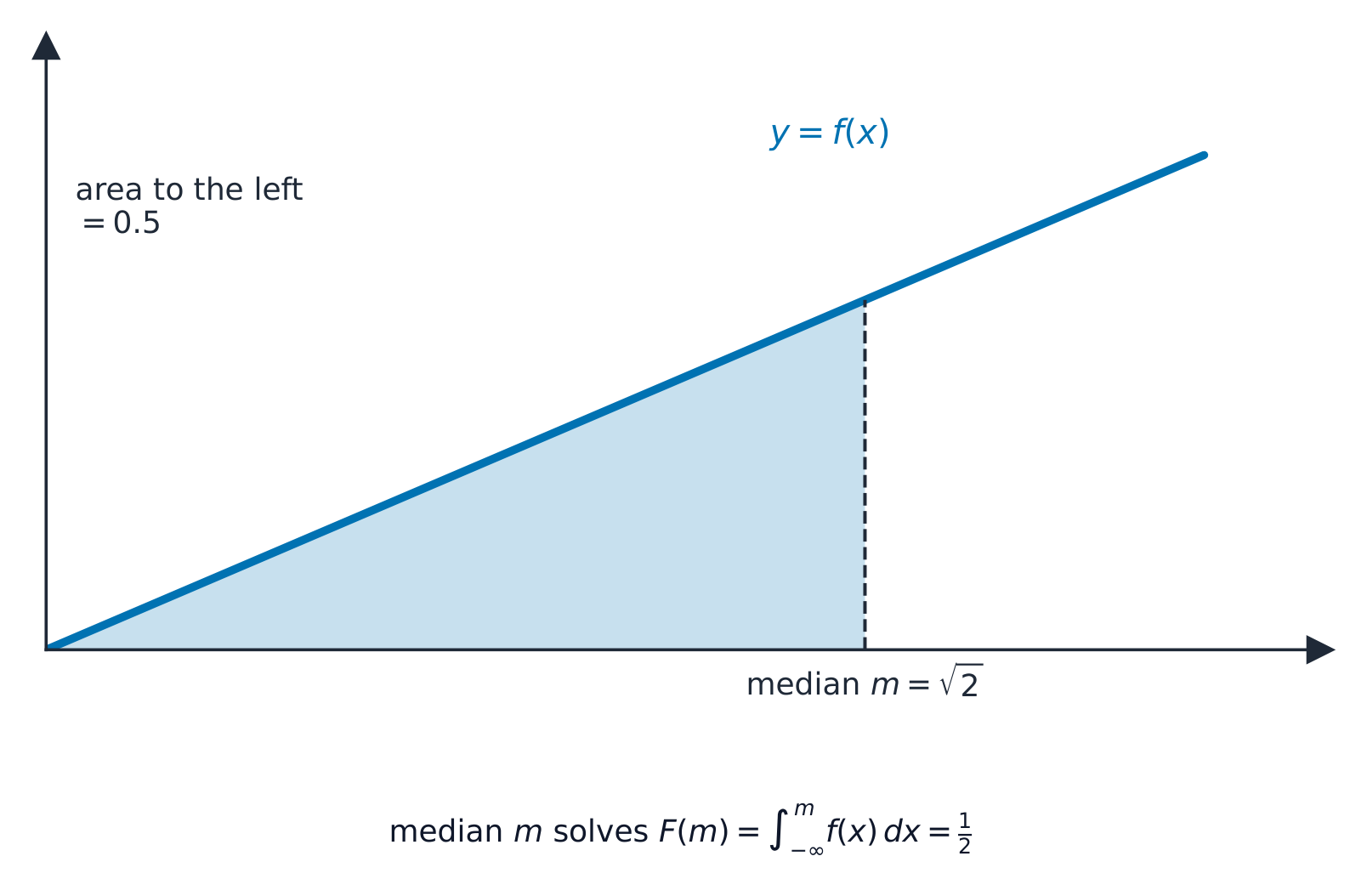
กราฟความหนาที่พื้นด้านซ้ายของค่ามัธยฐานถูกทาสีเทาเป็นครึ่งหนึ่ง
ค่ามัธยฐานอยู่ที่จุดที่พื้นที่ใต้ $f(x)$ ทางด้านซ้ายของมันเท่ากับ $0.5$ พอดี.

ฟังก์ชันการแจกแจงสะสม $F(x) = P(X \leqslant x)$ คือผลรวมสะสม: $F(x) = \displaystyle\int_{-\infty}^{x} f(t)\,dt$, และ $f(x) = F'(x)$. ใช้ $F$ เพื่อหาความน่าจะเป็นและ เปอร์เซ็นไทล์ (เช่น ค่ามัธยฐาน แก้สมการ $F(x) = 0.5$).

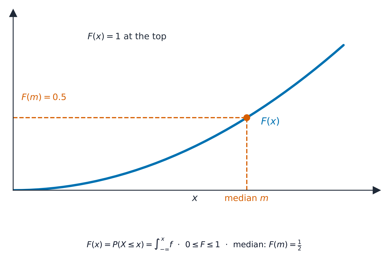
กราฟสะสมที่เพิ่มขึ้นจาก 0 ถึง 1 โดยอ่านค่ามัธยฐานที่ระดับสูง 0.5
กราฟสะสม $F(x)$ เพิ่มขึ้นจาก $0$ ไปยัง $1$; ระดับสูง $0.5$ ถูกเข้าถึงที่ค่ามัธยฐาน.

ตัวอย่างที่คำนวณแล้ว. ตัวแปรหนึ่งมี $f(x) = \tfrac12 x$ สำหรับ $0 \leqslant x \leqslant 2$. จงหาค่ามัธยฐาน

ฟังก์ชันการแจกแจงสะสมคือ $F(x) = \displaystyle\int_0^x \tfrac12 t\,dt = \tfrac14 x^2$. ตั้ง $F(m) = 0.5$:

$$\tfrac14 m^2 = 0.5 \;\Rightarrow\; m^2 = 2 \;\Rightarrow\; m = \sqrt{2} = 1.41.$$

การแจกแจงของตัวแปรที่เกี่ยวข้อง. ถ้า $Y=g(X)$, จงหาการแจกแจงของ $Y$ ผ่านฟังก์ชันสะสมของมัน. สำหรับ $Y=X^2$: $F_Y(y)=P(X^2\leqslant y)=P(-\sqrt y\leqslant X\leqslant\sqrt y)=F_X(\sqrt y)-F_X(-\sqrt y)$, แล้วหาอนุพันธ์เพื่อได้ $f_Y=F_Y'$. เมื่อ $g$ เป็นฟังก์ชันเพิ่มขึ้นอย่าง monotonic จะมีวิธีลัดคือ $F_Y(y)=F_X\big(g^{-1}(y)\big)$.

ตัวอย่างที่คำนวณแล้ว. เมื่อ $f_X(x)=\tfrac12 x$ บน $[0,2]$ (ดังนั้น $F_X(x)=\tfrac14 x^2$), ให้ $Y=X^2$. สำหรับ $0\leqslant y\leqslant 4$, $F_Y(y)=F_X(\sqrt y)=\tfrac14 y$, ดังนั้น $f_Y(y)=F_Y'(y)=\tfrac14$ – นั่นคือ $Y$ มีการแจกแจงแบบสม่ำเสมอบน $[0,4]$.

Explore · ⁨สำรวจ⁩

Continuous random variables · ⁨ตัวแปรสุ่มต่อเนื่อง⁩

P(a < X < b) = ∫ f(x) dx

For a continuous variable, probability is the area under the density curve. · ⁨สำหรับตัวแปรต่อเนื่อง ความน่าจะเป็นคือ พื้นที่ใต้เส้นโค้งความหนาแน่น⁩

Vocabulary · ⁨คำศัพท์⁩ Train · ⁨ฝึกฝน⁩
English ไทย
probability density function/ˌprɒbəˈbɪlɪti ˈdensɪti ˈfʌŋkʃn/ ฟังก์ชันความหนาแน่นความน่าจะเป็น
cumulative distribution function/ˈkjuːmjʊlətɪv ˌdɪstrɪˈbjuːʃn ˈfʌŋkʃn/ ฟังก์ชันการแจกแจงสะสม
percentiles/pəˈsentaɪlz/ percentiles
median/ˈmiːdiːən/ มัธยฐาน
hypothesis test/haɪˈpɒθəsɪs test/ การทดสอบสมมติฐาน
confidence interval/ˈkɒnfɪdəns ˈɪntəvl/ confidence interval
4.2

Inference using normal and t-distributions · ⁨การอนุมานโดยใช้การแจกแจงnormalและt⁩

Syllabus · ⁨หลักสูตร⁩
English
Candidates should be able to: Notes and examples
formulate hypotheses and apply a hypothesis test concerning the population mean using a small sample drawn from a normal population of unknown variance, using a t-test
calculate a pooled estimate of a population variance from two samples Calculations based on either raw or summarised data may be required.
formulate hypotheses concerning the difference of population means, and apply, as appropriate: - a 2-sample t-test - a paired sample t-test - a test using a normal distribution The ability to select the test appropriate to the circumstances of a problem is expected.
determine a confidence interval for a population mean, based on a small sample from a normal population with unknown variance, using a t-distribution
determine a confidence interval for a difference of population means, using a t-distribution or a normal distribution, as appropriate.
ไทย
ผู้เข้าสอบควรสามารถ: หมายเหตุและตัวอย่าง
ตั้งสมมติฐานและใช้ การทดสอบสมมติฐาน เกี่ยวกับค่าเฉลี่ยประชากร โดยใช้ตัวอย่างเล็กที่สุ่มมาจากประชากรที่มีการแจกแจงปกติที่มีความแปรปรวนไม่ทราบค่า โดยใช้ t-test
คำนวณ ค่าประมาณรวม ของความแปรปรวนประชากรจากตัวอย่างสองชุด อาจต้องการการคำนวณจากข้อมูลดิบหรือข้อมูลที่สรุปแล้ว
ตั้งสมมติฐานเกี่ยวกับผลต่างของค่าเฉลี่ยประชากร และใช้ตามความเหมาะสม: - t-test สำหรับตัวอย่าง 2 ชุด - t-test สำหรับตัวอย่างคู่ - การทดสอบที่ใช้ การแจกแจงปกติ คาดหวังว่าผู้เรียนจะสามารถเลือกการทดสอบที่เหมาะสมกับสถานการณ์ของปัญหา
กำหนด ช่วงความเชื่อมั่น สำหรับค่าเฉลี่ยประชากร โดยอ้างอิงจากตัวอย่างเล็กจากประชากรที่มีการแจกแจงปกติที่มีความแปรปรวนไม่ทราบค่า โดยใช้ การแจกแจง t
กำหนด ช่วงความเชื่อมั่น สำหรับผลต่างของค่าเฉลี่ยประชากร โดยใช้ การแจกแจง t หรือ การแจกแจงปกติ ตามความเหมาะสม

Source: Cambridge International syllabus · ⁨แหล่งที่มา: หลักสูตร Cambridge International⁩

English

When a sample is small and the population variance is unknown, base your hypothesis test 假设检验 on the $t$-distribution instead of the normal. The same idea gives a confidence interval 置信区间 for the mean:

$$\bar{x} \pm t\,\frac{s}{\sqrt{n}},$$
where $t$ comes from the $t$-tables with $n - 1$ degrees of freedom. To compare two populations, use a two-sample (2-sample) or paired-sample $t$-test, after finding a pooled estimate 合并估计 of the shared variance when appropriate.

Worked example. A sample of $n = 10$ has mean $\bar{x} = 50$ and standard deviation $s = 4$. Find a $95\%$ confidence interval for the mean (use $t = 2.262$ for $9$ degrees of freedom).

$$50 \pm 2.262\times\frac{4}{\sqrt{10}} = 50 \pm 2.86 \;\Rightarrow\; (47.1,\ 52.9).$$

ไทย
กระดานของ Galton ที่มีลูกบอลเรียงตัวเป็นรูป колокол
กระดานของ Galton: ลูกบอลที่ตกลงผ่านหมุดจะสะสมตัวเป็นรูป колокол ของการแจกแจงnormal.

เมื่อตัวอย่างมีขนาดเล็กและความแปรปรวนของประชากรไม่ทราบ ให้ใช้การทดสอบสมมติฐานบนการแจกแจง $t$ แทนที่จะเป็นnormal. แนวคิดเดียวกันนี้ให้ ช่วงความเชื่อมั่น สำหรับค่าเฉลี่ย:

$$\bar{x} \pm t\,\frac{s}{\sqrt{n}},$$
ซึ่ง $t$ มาจากตาราง $t$ ที่มี $n - 1$ องศาแห่งอิสรภาพ. เพื่อเปรียบเทียบประชากรสองกลุ่ม ให้ใช้การทดสอบ สองตัวอย่าง (two-sample) (2-sample) หรือการทดสอบ คู่ (paired-sample) $t$-test หลังจากหาค่าประมาณความแปรปรวนรวม (pooled estimate) ของความแปรปรวนร่วมกันเมื่อจำเป็นแล้ว.

กราฟการแจกแจงt که sitting ต่ำและกว้างกว่า standard normal
สำหรับตัวอย่างขนาดเล็ก การแจกแจง $t$ จะแบนลงและมีหางหนักกว่า ดังนั้นค่าวิกฤตจึงมีค่ามากกว่า

ตัวอย่างที่คำนวณแล้ว. ตัวอย่างขนาด $n = 10$ มีค่าเฉลี่ย $\bar{x} = 50$ และส่วนเบี่ยงเบนมาตรฐาน $s = 4$. จงหาช่วงความเชื่อมั่น $95\%$ สำหรับค่าเฉลี่ย (ใช้ $t = 2.262$ สำหรับ $9$ degrees of freedom).

$$50 \pm 2.262\times\frac{4}{\sqrt{10}} = 50 \pm 2.86 \;\Rightarrow\; (47.1,\ 52.9).$$

Explore · ⁨สำรวจ⁩

Why small samples need t instead of z · ⁨ทำไมตัวอย่างขนาดเล็กจึงต้องใช้ t แทน z⁩

With $\sigma$ unknown you use $t$, and $t$ has heavier tails than the normal (drawn dashed behind it) — so its critical values are larger and the interval is wider. At the worked example's $9$ degrees of freedom the widget reads $t^* = 2.262$, exactly the table value used above. Sweep df up and $t$ collapses onto the normal. · ⁨เมื่อ $\sigma$ ไม่ทราบใช้ $t$ และ $t$ มีหางหนากว่าปกติ (วาดด้วยเส้นประอยู่เบื้องหลัง) — ดังนั้นค่าวิกฤตจึง มากกว่า และช่วงมีความกว้างกว่า ที่ $9$ Degrees of freedom ของตัวอย่างที่คำนวณ Widget อ่านค่าได้ $t^* = 2.262$ ตรงกับค่าในตารางที่ใช้อ้างอิงข้างต้น ลาก df ขึ้นไปและ $t$ จะซ้อนทับกับกราฟปกติ⁩

Explore · ⁨สำรวจ⁩

The normal distribution · ⁨การแจกแจงปกติ⁩

Shade a tail to find a probability — the basis of confidence intervals and hypothesis tests. · ⁨แรเงาหางเพื่อหาค่าความน่าจะเป็น — เป็นพื้นฐานของช่วงความเชื่อมั่นและการทดสอบสมมติฐาน⁩

Vocabulary · ⁨คำศัพท์⁩ Train · ⁨ฝึกฝน⁩
English ไทย
pooled estimate/puːld ˈestɪmət/ ประมาณการรวม
degrees of freedom/dɪˈɡriːz ɒv ˈfriːdəm/ ระดับอิสระ
goodness of fit/ˈɡʊdnəs ɒv fɪt/ ความเหมาะสมของการแจกแจง (goodness of fit)
independence/ˌɪndɪˈpendəns/ ความเป็นอิสระ
contingency table/kənˈtɪndʒənsi ˈteɪbl/ ตารางความถี่ร่วม
4.3

Chi-squared tests · ⁨การทดสอบ Chi-squared⁩

Syllabus · ⁨หลักสูตร⁩
English
Candidates should be able to: Notes and examples
fit a theoretical distribution, as prescribed by a given hypothesis, to given data Questions will not involve lengthy calculations.
use a $\chi^2$-test, with the appropriate number of degrees of freedom, to carry out the corresponding goodness of fit analysis Classes should be combined so that each expected frequency is at least 5.
use a $\chi^2$-test, with the appropriate number of degrees of freedom, for independence in a contingency table. Yates’ correction is not required. Where appropriate, either rows or columns should be combined so that the expected frequency in each cell is at least 5.
ไทย
ผู้เข้าสอบควรสามารถ: หมายเหตุและตัวอย่าง
ปรับการแจกแจงทางทฤษฎีตามสมมติฐานที่กำหนดให้เข้ากับข้อมูลที่ได้รับ ข้อสอบจะไม่要求进行 lengthy calculations (การคำนวณที่ยาวนาน).
ใช้การทดสอบ $\chi^2$ ด้วยจำนวนองศาอิสระที่เหมาะสม เพื่อทำการวิเคราะห์ ความเหมาะสมของการปรับให้เข้ากัน (goodness of fit) ควรรวมกลุ่มเพื่อให้ค่าความถี่ที่คาดหวังของแต่ละกลุ่มมีอย่างน้อย 5.
ใช้การทดสอบ $\chi^2$ ด้วยจำนวนองศาอิสระที่เหมาะสม เพื่อตรวจสอบความเป็นอิสระใน ตารางความถ่วง (contingency table). ไม่จำเป็นต้องใช้การแก้ไขของ Yates. หากจำเป็น ให้รวมแถวหรือคอลัมน์เพื่อให้ค่าความถี่ที่คาดหวังในแต่ละเซลล์มีอย่างน้อย 5.

Source: Cambridge International syllabus · ⁨แหล่งที่มา: หลักสูตร Cambridge International⁩

English

A $\chi^2$-test (chi-squared test 卡方检验) compares observed counts $O$ with expected counts $E$ from a theoretical distribution 理论分布:

$$\chi^2 = \sum \frac{(O - E)^2}{E}.$$
Compare this with a table value for the right number of degrees of freedom 自由度. Two uses: a goodness of fit 拟合优度 test (does the data follow the proposed model?), and a test for independence 独立性 of two variables in a contingency table 列联表.

Worked example. Four equally likely categories give observed counts $20, 30, 25, 25$ (so each expected count is $25$). Test the fit at the $5\%$ level.

$$\chi^2 = \frac{(20-25)^2 + (30-25)^2 + 0 + 0}{25} = \frac{25 + 25}{25} = 2.$$
With $4 - 1 = 3$ degrees of freedom the table value is $7.815$. Since $2 < 7.815$, do not reject the model.

ไทย

การทดสอบ $\chi^2$ (chi-squared test) เปรียบเทียบจำนวนสังเกตได้ $O$ กับจำนวนคาดหวัง $E$ จาก การแจกแจงทฤษฎี:

$$\chi^2 = \sum \frac{(O - E)^2}{E}.$$
เปรียบเทียบกับค่าในตารางสำหรับจำนวน degrees of freedom ที่ถูกต้อง. ใช้งานสองแบบ: การทดสอบ ความเหมาะสมของการจัดวาง (ข้อมูลสอดคล้องกับโมเดลที่เสนอหรือไม่?) และการทดสอบ ความเป็นอิสระ ของตัวแปรสองตัวใน ตารางถ่วงน้ำหนัก

กราฟ chi-squared ที่เบี่ยงไปทางขวาพร้อมส่วนหาง 5% ด้านบนที่ถูกทาสีBeyond ค่าวิกฤต
การทดสอบปฏิเสธโมเดลเมื่อ $\chi^2$ เกินค่าวิกฤต ลงไปในส่วนหางสีเทา $5\%$

ตัวอย่างที่คำนวณแล้ว. สี่หมวดหมู่ที่มีความน่าเท่ากันให้จำนวนสังเกตได้ $20, 30, 25, 25$ (ดังนั้นจำนวนคาดหวังแต่ละอันคือ $25$). ทดสอบความเหมาะสมที่ระดับ $5\%$

$$\chi^2 = \frac{(20-25)^2 + (30-25)^2 + 0 + 0}{25} = \frac{25 + 25}{25} = 2.$$
ด้วย $4 - 1 = 3$ degrees of freedom ค่าในตารางคือ $7.815$. เนื่องจาก $2 < 7.815$, ไม่ปฏิเสธโมเดล

Explore · ⁨สำรวจ⁩

The chi-squared distribution and its 5% tail · ⁨การแจกแจง chi-squared และหาง 5%⁩

The worked example on this page gives $\chi^2 = 2$ with $3$ degrees of freedom against a table value of $7.815$ — the widget reproduces both. Drag df to see why the critical value changes with the number of categories. · ⁨ตัวอย่างที่คำนวณหน้านี้เป็น $\chi^2 = 2$ กับ $3$ Degrees of freedom เทียบกับค่าในตาราง $7.815$ — Widget นี้ทำซ้ำทั้งสองอย่าง ลาก df เพื่อดูว่าค่าวิกฤตเปลี่ยนตามจำนวนหมวดหมู่อย่างไร⁩

Explore · ⁨สำรวจ⁩

Chi-squared test route · ⁨เส้นทางทดสอบ Chi-squared⁩

Follow observed and expected counts to a test decision. · ⁨ติดตามจำนวนสังเกตและจำนวนคาดหวังไปสู่การตัดสินใจทดสอบ⁩

Vocabulary · ⁨คำศัพท์⁩ Train · ⁨ฝึกฝน⁩
English ไทย
chi-squared test/kaɪ skweəd test/ การทดสอบchi-squared
theoretical distribution/θɪəˈretɪkl ˌdɪstrɪˈbjuːʃn/ การแจกแจงทฤษฎี
4.4

Non-parametric tests · ⁨การทดสอบ Non-parametric⁩

Syllabus · ⁨หลักสูตร⁩
English
Candidates should be able to: Notes and examples
understand the idea of a non-parametric test and appreciate situations in which such a test might be useful e.g. when sampling from a population which cannot be assumed to be normally distributed.
understand the basis of the sign test, the Wilcoxon signed-rank test and the Wilcoxon rank-sum test Including knowledge that Wilcoxon tests are valid only for symmetrical distributions.
use a single-sample sign test and a single-sample Wilcoxon signed-rank test to test a hypothesis concerning a population median Including the use of normal approximations where appropriate. Questions will not involve tied ranks or observations equal to the population median value being tested.
use a paired-sample sign test, a Wilcoxon matched-pairs signed-rank test and a Wilcoxon rank-sum test, as appropriate, to test for identity of populations. Including the use of normal approximations where appropriate. Questions will not involve tied ranks or zero‑difference pairs.
ไทย
ผู้เข้าสอบควรสามารถ: หมายเหตุและตัวอย่าง
เข้าใจแนวคิดของการ ทดสอบแบบไม่มีพารามิเตอร์ และตระหนักถึงสถานการณ์ที่การทดสอบเช่นนี้อาจเป็นประโยชน์ เช่น เมื่อสุ่มตัวอย่างจากประชากรที่ไม่สามารถสันนิษฐานได้ว่ามีการแจกแจงแบบปกติ.
เข้าใจพื้นฐานของ การทดสอบเครื่องหมาย (sign test), การทดสอบ Wilcoxon แบบลงอันดับ (Wilcoxon signed-rank test) และ การทดสอบ Wilcoxon แบบรวมอันดับ (Wilcoxon rank-sum test) รวมถึงความรู้ว่าการทดสอบของ Wilcoxon จะใช้ได้กับเฉพาะการแจกแจงแบบสมมาตรเท่านั้น.
ใช้ การทดสอบเครื่องหมาย แบบตัวอย่างเดียวและ การทดสอบ Wilcoxon แบบลงอันดับ แบบตัวอย่างเดียว เพื่อทดสอบสมมติฐานเกี่ยวกับ มัธยฐาน ของประชากร รวมถึงการใช้ค่าประมาณด้วยฟังก์ชันปกติเมื่อเหมาะสม ข้อสอบจะไม่涉及 tied ranks (อันดับซ้ำ) หรือค่าสังเกตที่เท่ากับค่ามัธยฐานของประชากรที่กำลังทดสอบ.
ใช้ การทดสอบเครื่องหมาย แบบคู่, การทดสอบ Wilcoxon แบบจับคู่ (Wilcoxon matched-pairs signed-rank test) และ การทดสอบ Wilcoxon แบบรวมอันดับ ตามความเหมาะสม เพื่อทดสอบว่าประชากรมีเอกลักษณ์เดียวกันหรือไม่ รวมถึงการใช้ค่าประมาณด้วยฟังก์ชันปกติเมื่อเหมาะสม ข้อสอบจะไม่涉及 tied ranks (อันดับซ้ำ) หรือคู่ที่มีค่าต่างกันเป็นศูนย์.

Source: Cambridge International syllabus · ⁨แหล่งที่มา: หลักสูตร Cambridge International⁩

English

A non-parametric test 非参数检验 makes no assumption that the data is normal, so it is useful when that assumption fails. The basic ones are:

  • the sign test 符号检验: count how many values fall above and below a proposed median, and test those counts with a binomial model;
  • the Wilcoxon signed-rank test 威尔科克森符号秩检验 (the matched-pairs test for paired data), which also uses the sizes of the differences, not just their signs;
  • the Wilcoxon rank-sum test 威尔科克森秩和检验, for comparing two separate samples.

Worked example. Test whether a median is $5$. In a sample of $10$ values (none equal to $5$), $9$ lie above $5$ and $1$ lies below. Test at the $5\%$ level (two-tailed).

Under $H_0$ (median $= 5$) the number above follows $B(10, 0.5)$. The observed result ($9$ above) is extreme, so find $P(X \geq 9) = \binom{10}{9}(0.5)^{10} + (0.5)^{10} = \dfrac{11}{1024} = 0.0107$. For a two-tailed test compare with $\tfrac{1}{2}(5\%) = 0.025$. Since $0.0107 < 0.025$, reject $H_0$: there is evidence the median is not $5$.

ไทย

การทดสอบแบบไม่พารามิเตอร์ (non-parametric test) ไม่สมมติฐานว่าข้อมูลมีการแจกแจงปกติ ดังนั้นจึงมีประโยชน์เมื่อสมมติฐานดังกล่าวไม่เป็นจริง การทดสอบพื้นฐานมีดังนี้:

  • การทดสอบเครื่องหมาย (sign test): นับจำนวนค่าที่อยู่เหนือและต่ำกว่ามัธยฐานที่เสนอ แล้วทดสอบจำนวนเหล่านั้นด้วยโมเดลทวินาม;
  • การทดสอบWilcoxon signed-rank (การทดสอบคู่จับคู่สำหรับข้อมูลที่จับคู่กัน) ซึ่งใช้ขนาดของความแตกต่างไม่ใช่เพียงเครื่องหมายของความแตกต่าง;
  • การทดสอบWilcoxon rank-sum สำหรับเปรียบเทียบตัวอย่างอิสระสองกลุ่ม
เส้นจำนวนที่มีเส้นประแทนมัธยฐาน: จุดสามจุดด้านล่างมีเครื่องหมายลบ และสี่จุดด้านบนมีเครื่องหมายบวก
การทดสอบเครื่องหมายนับจำนวนค่าที่อยู่เหนือและต่ำกว่ามัธยฐานที่เสนอ จากนั้นทดสอบจำนวนเหล่านั้นด้วยโมเดลทวินาม

ตัวอย่างฝึกหัด. ทดสอบว่ามัธยฐานเป็น $5$ หรือไม่ ในตัวอย่าง $10$ ค่า (ไม่มีค่าเท่ากับ $5$), มี $9$ ค่าอยู่ เหนือ $5$ และมี $1$ ค่าอยู่ด้านล่าง ทดสอบที่ระดับ $5\%$ (สองหาง).

ภายใต้ $H_0$ (มัธยฐาน $= 5$) จำนวนค่าที่อยู่เหนือจะปฏิบัติตาม $B(10, 0.5)$. ผลลัพธ์ที่สังเกตได้ ($9$ ค่าอยู่เหนือ) เป็นค่าสุดขั้ว ดังนั้นให้หา $P(X \geq 9) = \binom{10}{9}(0.5)^{10} + (0.5)^{10} = \dfrac{11}{1024} = 0.0107$. สำหรับการทดสอบสองหาง ให้เปรียบเทียบกับ $\tfrac{1}{2}(5\%) = 0.025$. เนื่องจาก $0.0107 < 0.025$, ปฏิเสธ $H_0$: มีหลักฐานว่ามัธยฐานไม่ใช่ $5$.

Explore · ⁨สำรวจ⁩

Non-parametric test chooser · ⁨ผู้เลือกการทดสอบแบบไม่มีพารามิเตอร์⁩

Choose the rank-based test that matches the data situation. · ⁨เลือกการทดสอบที่อาศัยอันดับที่ตรงกับสถานการณ์ข้อมูล⁩

Vocabulary · ⁨คำศัพท์⁩ Train · ⁨ฝึกฝน⁩
English ไทย
non-parametric test/nɒn ˌpærəˈmetrɪk test/ การทดสอบแบบไม่พารามิเตอร์
sign test/saɪn test/ sign test
Wilcoxon signed-rank test/ˈwɪlkɒksn saɪnd ræŋk test/ การทดสอบ Wilcoxon signed-rank
Wilcoxon rank-sum test/ˈwɪlkɒksn ræŋk sʌm test/ การทดสอบ Wilcoxon rank-sum
probability generating function/ˌprɒbəˈbɪlɪti ˈdʒenəreɪtɪŋ ˈfʌŋkʃn/ ฟังก์ชันสร้างความน่าจะเป็น
Further Probability & Statistics/ˈfɜːðə ˌprɒbəˈbɪlɪti ænd stəˈtɪstɪks/ ความน่าจะเป็นและสถิติเพิ่มเติม
4.5

Probability generating functions · ⁨ฟังก์ชันสร้างโอกาส (probability generating functions)⁩

Syllabus · ⁨หลักสูตร⁩
English
Candidates should be able to: Notes and examples
understand the concept of a probability generating function (PGF) and construct and use the PGF for given distributions Including the discrete uniform, binomial, geometric and Poisson distributions.
use formulae for the mean and variance of a discrete random variable in terms of its PGF, and use these formulae to calculate the mean and variance of a given probability distribution
use the result that the PGF of the sum of independent random variables is the product of the PGFs of those random variables.
ไทย
ผู้เข้าสอบควรสามารถ: หมายเหตุและตัวอย่าง
เข้าใจแนวคิดของ ฟังก์ชันสร้าง peluang (PGF) และสร้างและใช้ PGF สำหรับการแจกแจงที่กำหนดให้ รวมถึงการแจกแจงแบบสม่ำเสมอแบบไม่ต่อเนื่อง, แบบไบนอม, แบบเรขาคณิต และแบบปอยซง.
ใช้สูตรสำหรับค่าเฉลี่ยและความแปรปรวนของตัวแปรสุ่มแบบไม่ต่อเนื่องในรูปของ PGF และใช้สูตรเหล่านี้เพื่อคำนวณค่าเฉลี่ยและความแปรปรวนของการแจกแจง peluangที่กำหนดให้
ใช้ผลลัพธ์ที่ว่า PGF ของผลบวกของตัวแปรสุ่มที่เป็นอิสระต่อกันคือผลคูณของ PGF ของตัวแปรสุ่มเหล่านั้น.

Source: Cambridge International syllabus · ⁨แหล่งที่มา: หลักสูตร Cambridge International⁩

English

The probability generating function 概率母函数 of a discrete variable $X$ is

$$G(t) = E(t^X) = \sum_x P(X = x)\,t^x.$$
It packs the whole distribution into one function. The mean and variance come from its derivatives at $t = 1$: $E(X) = G'(1)$ and $\mathrm{Var}(X) = G''(1) + G'(1) - \big(G'(1)\big)^2$. Also, the PGF of a sum of independent variables is the product of their PGFs.

Worked example. $X$ has $P(X=0) = 0.5$, $P(X=1) = 0.3$, $P(X=2) = 0.2$. Find $E(X)$ using the PGF.

Here $G(t) = 0.5 + 0.3t + 0.2t^2$, so $G'(t) = 0.3 + 0.4t$ and

$$E(X) = G'(1) = 0.3 + 0.4 = 0.7.$$

ไทย
ลูกเต๋าหลายชนิด
ลูกเต๋า: จุดเริ่มต้นของการคำนวณโอกาสและตัวแปรสุ่มแบบไม่ต่อเนื่อง.

ฟังก์ชันสร้างโอกาสของตัวแปรไม่ต่อเนื่อง $X$ คือ

$$G(t) = E(t^X) = \sum_x P(X = x)\,t^x.$$
มันรวมการแจกแจงทั้งหมดไว้ในฟังก์ชันเดียว ค่าเฉลี่ยและความแปรปรวนหาได้จากอนุพันธ์ที่ $t = 1$: $E(X) = G'(1)$ และ $\mathrm{Var}(X) = G''(1) + G'(1) - \big(G'(1)\big)^2$. นอกจากนี้ PGF ของผลรวมของตัวแปรอิสระคือผลคูณของ PGF ของตัวแปรเหล่านั้น

ตัวอย่างฝึกหัด. $X$ มี $P(X=0) = 0.5$, $P(X=1) = 0.3$, $P(X=2) = 0.2$. หา $E(X)$ โดยใช้ PGF.

ที่นี่ $G(t) = 0.5 + 0.3t + 0.2t^2$, ดังนั้น $G'(t) = 0.3 + 0.4t$ และ

$$E(X) = G'(1) = 0.3 + 0.4 = 0.7.$$

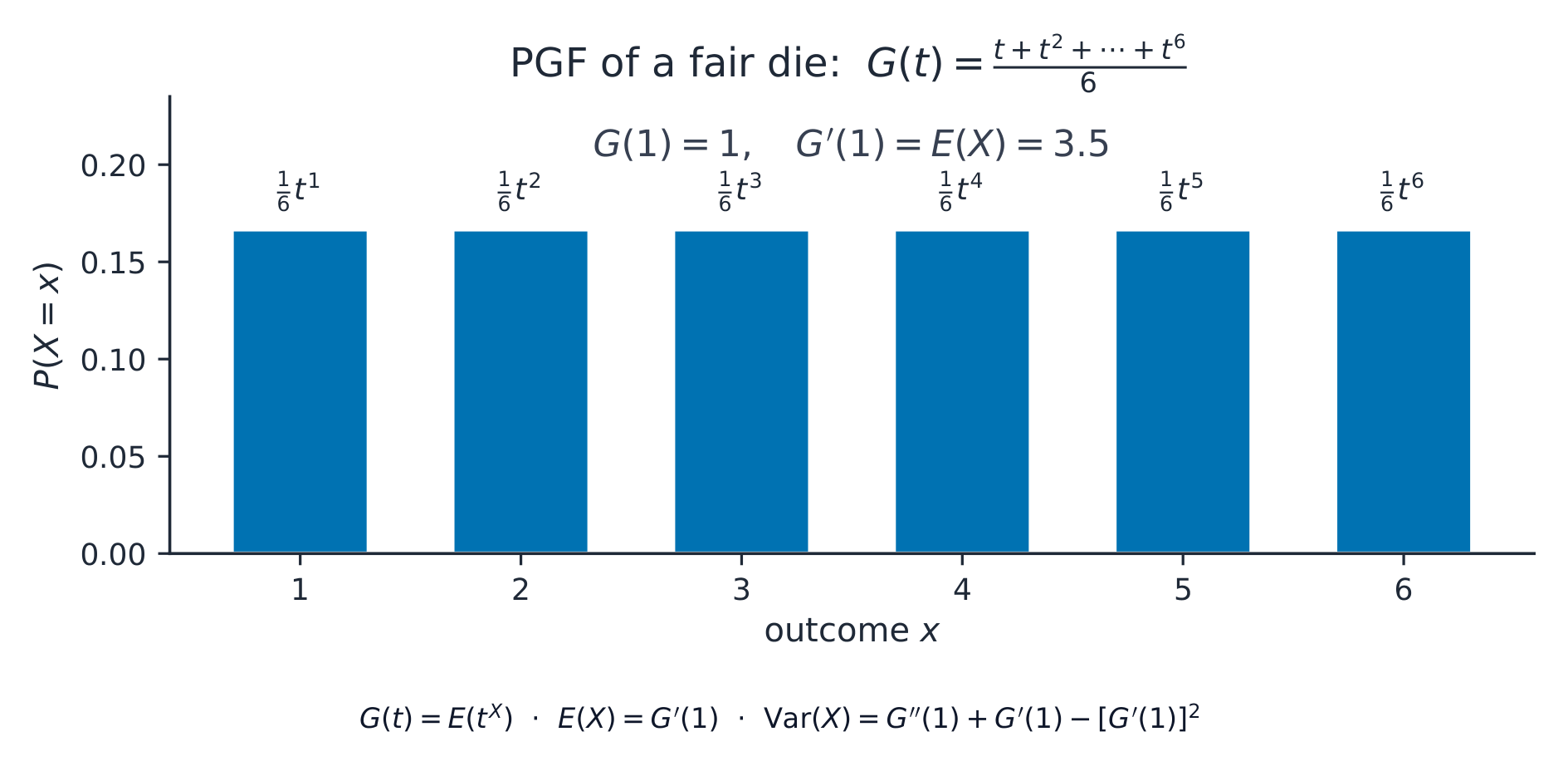
PGF ของลูกเต๋าสุ่มจัดมวลเท่ากันที่ 1 ถึง 6 ลงใน G(t)
PGF ของลูกเต๋าสัมผัสรวมมวลเท่ากันที่ 1 ถึง 6 ไว้ใน G(t)
Explore · ⁨สำรวจ⁩

Probability generating function lab · ⁨ห้องปฏิบัติการฟังก์ชันสร้างความน่าจะเป็น⁩

G(x) = p0 + p1 x + p2 x^2 + ...

Change x and see how a PGF stores probabilities in powers of x. · ⁨เปลี่ยน x และดูว่า PGF เก็บความน่าจะเป็นในกำลังของ x อย่างไร⁩

4.5

Exam tips · ⁨ข้อแนะนำสำหรับการสอบ⁩

English
  • For a continuous random variable, the pdf integrates to $1$ over its range, and $E(X) = \int x f(x)\,dx$.
  • Use the $t$-distribution when the sample is small and the population variance is unknown; state the degrees of freedom.
  • For a chi-squared test compute $\sum (O-E)^2/E$, compare with the critical value at the right degrees of freedom, and combine classes with $E < 5$.
  • State $H_0$ and $H_1$ and give the conclusion in context for every test.
ไทย
  • สำหรับ ตัวแปรสุ่มต่อเนื่อง, pdf จะอินทิเกรตได้ $1$ ในช่วงของตัวแปร, และ $E(X) = \int x f(x)\,dx$.
  • ใช้ การแจกแจง$t$ เมื่อตัวอย่างมีขนาดเล็กและความแปรปรวนของประชากรไม่ทราบ; ระบุองศาอิสระ
  • สำหรับการทดสอบ chi-squared คำนวณ $\sum (O-E)^2/E$, เปรียบเทียบกับค่าวิกฤตที่องศาอิสระทางขวา, และ รวมคลาสที่มี $E < 5$
  • ระบุ $H_0$ และ $H_1$ และให้ข้อสรุป ในบริบท สำหรับทุกการทดสอบ

Interactive lessons on this topic · ⁨บทเรียนเชิงโต้ตอบสำหรับหัวข้อนี้⁩

Work through it step by step, with instant-check exercises. · ⁨ทำทีละขั้นตอน พร้อมแบบฝึกหัดตรวจสอบผลทันที⁩

Past Papers · ⁨ข้อสอบย้อนหลัง⁩

More topics in A-Level Further Mathematics · ⁨Further Mathematics A-Level⁩ · ⁨หัวข้อเพิ่มเติมใน A-Level Further Mathematics · ⁨Further Mathematics A-Level⁩⁩

Log in or create account · ⁨เข้าสู่ระบบหรือสร้างบัญชี⁩

IGCSE, A-Level & AP