Further Pure Mathematics 1

For a polynomial equation, the roots 根 are linked to the coefficients 系数. For $ax^2 + bx + c = 0$ with roots $\alpha, \beta$:

For a cubic $ax^3 + bx^2 + cx + d = 0$ with roots $\alpha, \beta, \gamma$: Sums like $\sum\alpha$ and $\sum\alpha\beta$ are symmetric functions 对称函数 of the roots (unchanged if the roots are swapped). To find an equation whose roots are changed in a simple way, use a substitution 代换 (for example, put $w = \alpha + 1$).

Worked example. The equation $x^2 - 5x + 6 = 0$ has roots $\alpha, \beta$. Find the equation with roots $\alpha + 1, \beta + 1$.

Here $\alpha + \beta = 5$ and $\alpha\beta = 6$. The new sum is $(\alpha + 1) + (\beta + 1) = 7$, and the new product is $(\alpha + 1)(\beta + 1) = \alpha\beta + \alpha + \beta + 1 = 6 + 5 + 1 = 12$. So the new equation is

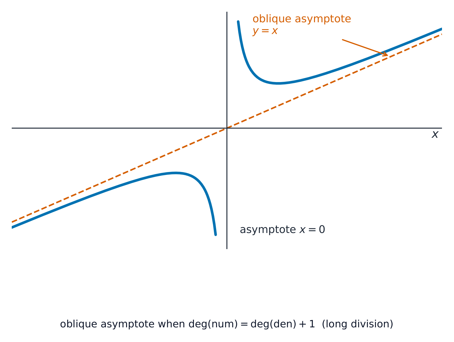
A rational function 有理函数 is a fraction of two polynomials. When the top has higher degree than the bottom, the graph has an oblique asymptote 斜渐近线 (a slanted line the curve approaches); find it by dividing out. You should also be able to relate the graph of $y = f(x)$ to those of $y^2 = f(x)$, $y = \dfrac{1}{f(x)}$, $y = |f(x)|$ and $y = f(|x|)$. Find the set of values the function can take using the discriminant 判别式, and locate its turning points 驻点.

Far from the origin the curve hugs the slant line $y=x$; near $x=0$ it runs off along the vertical asymptote.

Worked example. Find the oblique asymptote of $y = \dfrac{x^2 + x + 1}{x + 1}$.

Divide out the fraction: $\dfrac{x^2 + x + 1}{x + 1} = x + \dfrac{1}{x + 1}$. As $x \to \pm\infty$ the remainder $\dfrac{1}{x+1} \to 0$, so the curve approaches the line $y = x$ — the oblique asymptote.

Learn the standard results:

The method of differences 差分法 sums a series by cancelling middle terms: if partial fractions 部分分式 write each term as $f(r) - f(r+1)$, almost everything cancels. From the sum to $n$ terms you can see whether a series is convergent 收敛 and, if so, find its sum to infinity 无穷和.

Worked example. Find $\displaystyle\sum_{r=1}^{n} (2r + 1)$.

A matrix 矩阵 is a rectangular block of numbers. Matrix addition adds entries in matching positions; you can also subtract and multiply matrices (multiplication is row $\times$ column). The zero matrix 零矩阵 has every entry $0$, and the identity matrix 单位矩阵 (or unit matrix) $I$ leaves any matrix unchanged under multiplication.

For a $2\times 2$ matrix $A = \begin{pmatrix} a & b \\ c & d \end{pmatrix}$, the determinant 行列式 is $\det A = ad - bc$. If $\det A \neq 0$ the matrix is non-singular (otherwise it is a singular matrix 奇异矩阵), and the inverse matrix 逆矩阵 is

For a product, $(AB)^{-1} = B^{-1}A^{-1}$. A $2\times 2$ matrix can represent a geometric transformation 几何变换 of the plane — a rotation 旋转, reflection 反射, enlargement 放大, stretch 拉伸 or shear 切变: the determinant gives the area scale factor, and a product $AB$ means "do $B$, then $A$". Points or lines that do not move are called invariant points 不变点 and invariant lines 不变直线.

The matrix sends the unit square to a parallelogram whose area is the determinant.

Worked example. Find the inverse of $A = \begin{pmatrix} 3 & 1 \\ 2 & 4 \end{pmatrix}$.

$\det A = 3\times 4 - 1\times 2 = 10$, so

A spiral staircase: spirals are described naturally using polar coordinates.

Polar coordinates 极坐标 give a point by its distance $r$ from the origin and its angle $\theta$. They link to Cartesian coordinates 直角坐标 by

Polar coordinates $(r,\theta)$ convert to Cartesian by $x=r\cos\theta$ and $y=r\sin\theta$.

You should sketch simple polar curves 极坐标曲线, and find the area of a sector with

The cardioid $r=1+\cos\theta$, plotted straight from $r$ as a function of $\theta$.

Worked example. Convert the polar equation $r = 4\cos\theta$ to Cartesian form.

Multiply both sides by $r$: $r^2 = 4r\cos\theta$, so $x^2 + y^2 = 4x$. Completing the square gives $(x - 2)^2 + y^2 = 4$, a circle of radius $2$ centred at $(2, 0)$.

Forces like wind and water are vectors — they have both size and direction.

In three dimensions a plane 平面 can be written as $ax + by + cz = d$, or $\mathbf{r}\cdot\mathbf{n} = p$, or $\mathbf{r} = \mathbf{a} + \lambda\mathbf{b} + \mu\mathbf{c}$. Besides the scalar product, there is the vector product 向量积 of two vectors 向量:

which gives a vector at right angles to both. With scalar and vector products you can find distances, angles, and where lines and planes meet — including the shortest distance between skew lines 异面直线.

$\mathbf{a}\times\mathbf{b}$ is perpendicular to both vectors; its length equals the area of the parallelogram they span.

Worked example. Find $\mathbf{a}\times\mathbf{b}$ for $\mathbf{a} = \mathbf{i} + \mathbf{j}$ and $\mathbf{b} = \mathbf{j} + \mathbf{k}$.

Mathematical induction 数学归纳法 proves a result for every positive integer $n$ in two steps:

1. Base case: show the result is true for $n = 1$.
2. Inductive step: assume it is true for $n = k$, then prove it for $n = k + 1$.

If both steps work, the result is true for all $n$. Often you first make a conjecture 猜想 (a sensible guess) from a few cases, then confirm it by inductive proof 归纳证明.

Induction is like dominoes: the base case topples the first, and the inductive step makes each one knock over the next — so the result holds for every n

Worked example. Prove that $\displaystyle\sum_{r=1}^{n} r = \tfrac12 n(n+1)$.

Base case $n = 1$: the left side is $1$ and the right side is $\tfrac12(1)(2) = 1$. True. Inductive step: assume $\displaystyle\sum_{r=1}^{k} r = \tfrac12 k(k+1)$. Then

This is the formula with $n = k + 1$, so by induction it holds for all $n$.

• Use the relationships between roots and coefficients (sum, sum of pairs, product) instead of solving the polynomial.
• For proof by induction, set out the base case, assume the result for $n = k$, prove it for $n = k+1$, and write a clear closing statement.
• Sketch rational-function graphs with their asymptotes and turning points; use the method of differences for a summation.
• For matrices, know the determinant, inverse and invariant lines, and interpret each transformation geometrically.