Further Pure Mathematics 2

A hanging cable forms a catenary — the curve of the hyperbolic cosine.

The hyperbolic functions 双曲函数 are built from the exponential function:

$\cosh$ is the average of $e^x$ and $e^{-x}$; $\sinh$ is half their difference.

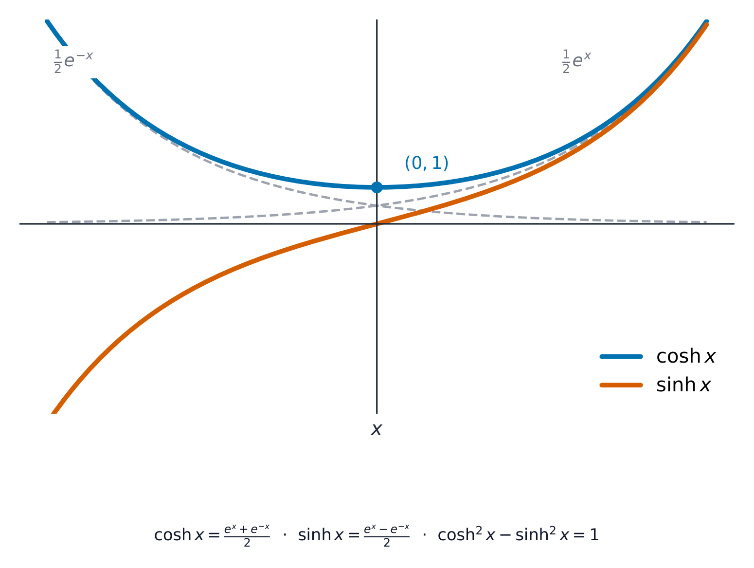
They obey identities much like the trigonometric ones, the main one being $\cosh^2 x - \sinh^2 x = 1$. The three reciprocals complete the set: $\operatorname{sech} x = \dfrac{1}{\cosh x}$, $\operatorname{cosech} x = \dfrac{1}{\sinh x}$, and $\coth x = \dfrac{1}{\tanh x} = \dfrac{\cosh x}{\sinh x}$ – all built from $e^x$ too, and worth recognising in integrals and mark schemes. The inverse hyperbolic functions 反双曲函数 have a logarithmic form 对数形式, for example $\sinh^{-1} x = \ln\!\left(x + \sqrt{x^2 + 1}\right)$.

Worked example. Show that $\cosh^2 x - \sinh^2 x = 1$.

You can write three linear equations in three unknowns as a single matrix equation 矩阵方程 $A\mathbf{x} = \mathbf{b}$. If $A$ is non-singular there is one solution; if $A$ is singular the equations are either inconsistent (no solution) or have infinitely many.

For a square matrix $A$, the characteristic equation 特征方程 is $\det(A - \lambda I) = 0$. Its solutions are the eigenvalues 特征值 $\lambda$, and for each one the vector $\mathbf{v}$ with $A\mathbf{v} = \lambda\mathbf{v}$ is an eigenvector 特征向量. You can then write $A = QDQ^{-1}$, where $D$ is a diagonal matrix 对角矩阵 of eigenvalues and the columns of $Q$ are the eigenvectors.

Multiplying an eigenvector by $A$ only stretches it; a general vector is turned to a new direction.

Worked example. Find the eigenvalues of $A = \begin{pmatrix} 2 & 1 \\ 1 & 2 \end{pmatrix}$.

The characteristic equation is

So $\lambda = 1$ or $\lambda = 3$. (The eigenvector for $\lambda = 3$ is $\begin{pmatrix} 1 \\ 1 \end{pmatrix}$ and for $\lambda = 1$ is $\begin{pmatrix} 1 \\ -1 \end{pmatrix}$.)

You can now differentiate the hyperbolic functions and the inverse functions $\sin^{-1}x$, $\tan^{-1}x$, $\sinh^{-1}x$ and so on. You can also find $\dfrac{d^2y}{dx^2}$ for curves given implicitly or parametrically.

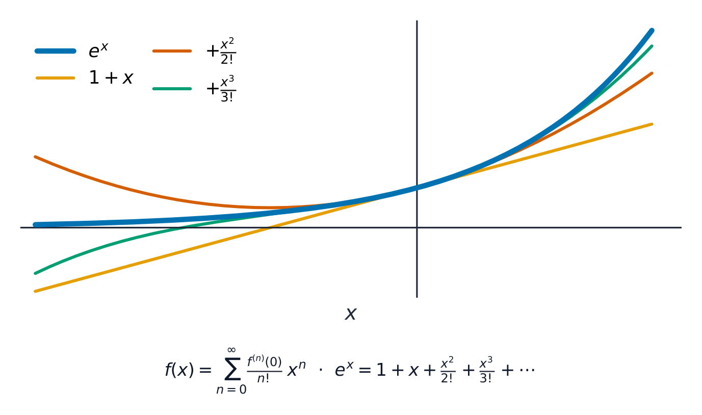
A Maclaurin's series 麦克劳林级数 writes a function as a power series:

For example $e^x = 1 + x + \dfrac{x^2}{2!} + \dfrac{x^3}{3!} + \cdots$

Adding more terms makes the polynomial match $e^x$ over a wider stretch around $x=0$.

Worked example. Find the Maclaurin series of $f(x) = \ln(1+x)$ up to the term in $x^3$.

$f(0) = 0$; $f'(x) = \dfrac{1}{1+x}$ so $f'(0) = 1$; $f''(x) = \dfrac{-1}{(1+x)^2}$ so $f''(0) = -1$; $f'''(x) = \dfrac{2}{(1+x)^3}$ so $f'''(0) = 2$. Substituting into the series:

Learn these standard integrals:

A trigonometric substitution, a hyperbolic substitution, or completing the square 配方法 in the denominator handles related forms. A reduction formula 递推公式 links an integral $I_n$ to $I_{n-1}$, so you can work down step by step. Integration also gives the arc length 弧长 of a curve and the surface area of revolution 旋转曲面面积 when a curve is turned about an axis.

Worked example. Find $\displaystyle\int \frac{1}{\sqrt{4 - x^2}}\,dx$.

Here $a^2 = 4$, so $a = 2$ and

Bounding a sum by an integral. Draw rectangles of unit width under, or over, a decreasing curve such as $y=\frac1x$. Each rectangle of height $\frac1r$ is trapped between two integral strips, so summing gives

Shrinking the rectangle width to $\frac1n\to 0$ turns such a sum into a Riemann sum 黎曼和 that equals the integral in the limit, e.g. $\displaystyle\lim_{n\to\infty}\frac1n\sum_{r=1}^{n}f\!\left(\frac{r}{n}\right)=\int_0^1 f(x)\,dx$.

Self-similar patterns like Romanesco broccoli arise from iterating functions in the complex plane.

A complex number 复数 in polar form is $z = r(\cos\theta + i\sin\theta)$. De Moivre's theorem 棣莫弗定理 says that for any integer $n$,

It is used to expand $\cos n\theta$ and $\sin n\theta$ in powers, to sum series, and to find the $n$ roots of unity 单位根 (the solutions of $z^n = 1$, equally spaced around the unit circle).

The five solutions of $z^5=1$ are equally spaced $72^\circ$ apart on the unit circle.

Worked example. Use de Moivre's theorem to express $\cos 3\theta$ in terms of $\cos\theta$.

Take the real part of $(\cos\theta + i\sin\theta)^3 = \cos 3\theta + i\sin 3\theta$:

For a first order linear equation $\dfrac{dy}{dx} + P(x)\,y = Q(x)$, multiply by the integrating factor 积分因子 $\mu = e^{\int P\,dx}$. The left side then becomes $\dfrac{d}{dx}(\mu y)$, so you can integrate directly.

For a linear equation with constant coefficients, the general solution 通解 is the sum of two parts: the complementary function 余函数 (the solution of the equation with the right side set to $0$, found from the auxiliary equation) and a particular integral 特积分 (any one solution of the full equation). Initial conditions then fix the constants to give the particular solution 特解; simpler equations with separable variables 可分离变量 are integrated directly.

A solution curve follows the slope field, staying tangent to the little segments everywhere.

Worked example. Solve $\dfrac{dy}{dx} + 2y = e^x$.

The integrating factor is $\mu = e^{\int 2\,dx} = e^{2x}$. Multiplying through gives $\dfrac{d}{dx}\!\left(y\,e^{2x}\right) = e^{3x}$, so

Second order, constant coefficients. For $\dfrac{d^2y}{dx^2}+b\dfrac{dy}{dx}+cy=f(x)$, solve the auxiliary equation 辅助方程 $m^2+bm+c=0$. The complementary function depends on its roots:

• two distinct real roots $m_1,m_2$: $y=Ae^{m_1x}+Be^{m_2x}$;
• a repeated root $m$: $y=(A+Bx)e^{mx}$;
• complex roots $p\pm qi$: $y=e^{px}(A\cos qx+B\sin qx)$.

Then add a particular integral by trying a form matching $f(x)$ (a polynomial, $ae^{bx}$, or $a\cos px+b\sin px$); if that trial already appears in the complementary function, multiply it by $x$.

Worked example. Solve $\dfrac{d^2y}{dx^2}-4\dfrac{dy}{dx}+4y=0$. The auxiliary equation $m^2-4m+4=(m-2)^2=0$ has a repeated root $m=2$, so $y=(A+Bx)e^{2x}$.

• Learn the hyperbolic identities and derivatives, and use the inverse hyperbolic functions in integration.
• Solve a linear differential equation as complementary function $+$ particular integral, then apply the boundary conditions.
• Use de Moivre's theorem for powers and roots of complex numbers and to derive trigonometric identities.
• Reduce an integral to a standard form by a stated substitution.