Статистический вывод для категориальных данных: доли
Город хочет узнать, сколько людей поддерживает новую политику. Мы не можем спросить всех, поэтому случайно опрашиваем двухсот. Сто двадцать говорят «да» — шестьдесят…
English narration · English + 中文 subtitles burned in · Английское озвучивание · Английский + китайские субтитры (встроенные)
6.1
Why Be Normal? · Почему нужна нормальность?
Syllabus · Программа
English
Enduring Understanding (VAR-1): Given that variation may be random or not, conclusions are uncertain.
Learning Objective VAR-1.H: Identify questions suggested by variation in the shapes of distributions of samples taken from the same population. [Skill 1.A]
VAR-1.H.1 Variation in shapes of data distributions may be random or not.
Русский
Вечная идея (VAR-1): Поскольку вариация может быть случайной или нет, выводы остаются неопределенными.
Цель обучения VAR-1.H: Определять вопросы, возникающие из вариации форм распределений выборок, взятых из одной и той же генеральной совокупности. [Навык 1.A]
VAR-1.H.1 Вариация форм распределений данных может быть случайной или неслучайной.
Source: College Board AP Course and Exam Description · Источник: Описание курса и экзамена College Board AP
English
Because a sample proportion $\hat{p}$ is approximately normally distributed (when the conditions hold), we can measure how far a sample result is from a claimed value in standard errors, and turn that into a probability. This is what makes inference 推断 – drawing conclusions about a population from a sample – possible.
Русский
Поскольку выборочная доля $\hat{p}$ приблизительно нормально распределена (при выполнении условий), мы можем измерить, насколько результат выборки отклоняется от заявленного значения в единицах стандартной ошибки, и преобразовать это в вероятность. Именно это делает возможным статистический вывод — формулирование заключений о генеральной совокупности на основе выборки.
6.2
Confidence Interval for a Proportion · Доверительный интервал для доли
Syllabus · Программа
English
Enduring Understanding (UNC-4): An interval of values should be used to estimate parameters, in order to account for uncertainty.
Learning Objective UNC-4.A: Identify an appropriate confidence interval procedure for a population proportion. [Skill 1.D]
UNC-4.A.1 The appropriate confidence interval procedure for a one-sample proportion for one categorical variable is a one sample $z$-interval for a proportion.
Learning Objective UNC-4.B: Verify the conditions for calculating confidence intervals for a population proportion. [Skill 4.C]
UNC-4.B.1 In order to make assumptions necessary for inference on population proportions, means, and slopes, we must check for independence in data collection methods and for selection of the appropriate sampling distribution.
UNC-4.B.2 In order to calculate a confidence interval to estimate a population proportion, $p$, we must check for independence and that the sampling distribution is approximately normal.
a. To check for independence:
i. Data should be collected using a random sample or a randomized experiment.
ii. When sampling without replacement, check that $n \leq 10\%N$, where $N$ is the size of the population.
b. To check that the sampling distribution of $\hat{p}$ is approximately normal (shape):
i. For categorical variables, check that both the number of successes, $n\hat{p}$, and the number of failures, $n(1-\hat{p})$ are at least 10 so that the sample size is large enough to support an assumption of normality.
Learning Objective UNC-4.C: Determine the margin of error for a given sample size and an estimate for the sample size that will result in a given margin of error for a population proportion. [Skill 3.D]
UNC-4.C.1 Based on sample data, the standard error of a statistic is an estimate for the standard deviation for the statistic. The standard error of $\hat{p}$ is $SE_{\hat{p}} = \sqrt{\dfrac{\hat{p}(1-\hat{p})}{n}}$.
UNC-4.C.2 A margin of error gives how much a value of a sample statistic is likely to vary from the value of the corresponding population parameter.
UNC-4.C.3 For categorical variables, the margin of error is the critical value ($z^*$) times the standard error (SE) of the relevant statistic, which equals $z^* \sqrt{\dfrac{\hat{p}(1-\hat{p})}{n}}$ for a one sample proportion.
UNC-4.C.4 The formula for margin of error can be rearranged to solve for $n$, the minimum sample size needed to achieve a given margin of error. For this purpose, use a guess for $\hat{p}$ or use $\hat{p} = 0.5$ in order to find an upper bound for the sample size that will result in a given margin of error.
Learning Objective UNC-4.D: Calculate an appropriate confidence interval for a population proportion. [Skill 3.D]
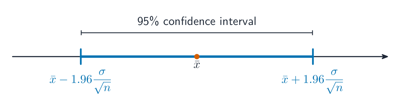
UNC-4.D.1 In general, an interval estimate can be constructed as point estimate ± (margin of error). For a one-sample proportion, the interval estimate is $\hat{p} \pm z^* \sqrt{\dfrac{\hat{p}(1-\hat{p})}{n}}$.
Clarifying statement: Formulas for interval estimates do not appear explicitly on the AP Statistics Formula Sheet provided with the AP Statistics Exam. However, these formulas do not need to be memorized, as they can be constructed based on the general test statistic formula and the relevant standard error formulas that are provided on the formula sheet.
UNC-4.D.2 Critical values represent the boundaries encompassing the middle C% of the standard normal distribution, where C% is an approximate confidence level for a proportion.
Learning Objective UNC-4.E: Calculate an interval estimate based on a confidence interval for a population proportion. [Skill 3.D]
UNC-4.E.1 Confidence intervals for population proportions can be used to calculate interval estimates with specified units.
Русский
Продолжающееся понимание (UNC-4): Доверительный интервал значений следует использовать для оценки параметров, чтобы учесть неопределенность.
Цель обучения UNC-4.A: Определить подходящий процедуру построения доверительного интервала для генеральной пропорции. [Навык 1.D]
UNC-4.A.1 Подходящей процедурой построения доверительного интервала для одновыборочной пропорции по одной категориальной переменной является одновыборочный $z$-интервал для пропорции.
Цель обучения UNC-4.B: Проверять условия для расчета доверительных интервалов для генеральной пропорции. [Навык 4.C]
UNC-4.B.1 Чтобы сделать допущения, необходимые для статистического вывода относительно долей населения, средних значений и угловых коэффициентов, необходимо проверить независимость методов сбора данных и выбор соответствующего сэмплируемого распределения.
UNC-4.B.2 Чтобы рассчитать доверительный интервал для оценки доли населения $p$, мы должны проверить независимость и то, что сэмплируемое распределение приблизительно нормально.
a. Для проверки независимости:
i. Данные следует собирать с использованием случайной выборки или рандомизированного эксперимента.
ii. При выборке без возвращения проверьте, что $n \leq 10\%N$, где $N$ — это размер генеральной совокупности.
b. Для проверки того, что выборочное распределение $\hat{p}$ приближенно нормально (форма):
i. Для категориальных переменных проверьте, что как количество успехов, $n\hat{p}$, так и количество неудач, $n(1-\hat{p})$, составляют не менее 10, чтобы размер выборки был достаточным для поддержания предположения о нормальности.
Цель обучения UNC-4.C: Определить погрешность выборки для заданного размера выборки и оценку размера выборки, которая приведет к заданной погрешности выборки для доли населения. [Навык 3.D]
UNC-4.C.1 На основе выборочных данных стандартная ошибка статистики является оценкой стандартного отклонения для этой статистики. Стандартная ошибка $\hat{p}$ равна $SE_{\hat{p}} = \sqrt{\dfrac{\hat{p}(1-\hat{p})}{n}}$.
UNC-4.C.2 Погрешность выборки показывает, насколько значение выборочной статистики может отличаться от значения соответствующего параметра генеральной совокупности.
UNC-4.C.3 Для категориальных переменных погрешность выборки равна критическому значению ($z^*$), умноженному на стандартную ошибку (SE) соответствующей статистики, которая равна $z^* \sqrt{\dfrac{\hat{p}(1-\hat{p})}{n}}$ для одной выборочной доли.
UNC-4.C.4 Формулу погрешности выборки можно преобразовать для решения относительно $n$ — минимального размера выборки, необходимого для достижения заданной погрешности выборки. Для этой цели используйте предположение для $\hat{p}$ или примените $\hat{p} = 0.5$, чтобы найти верхнюю границу размера выборки, которая приведет к заданной погрешности выборки.
Цель обучения UNC-4.D: Рассчитать подходящий доверительный интервал для доли населения. [Навык 3.D]
UNC-4.D.1 В целом точечную оценку можно построить как: точечная оценка ± (погрешность выборки). Для одной выборочной доли точечная оценка имеет вид $\hat{p} \pm z^* \sqrt{\dfrac{\hat{p}(1-\hat{p})}{n}}$.
Уточняющее замечание: Формулы для точечных оценок явно не приводятся в Листе формул AP Statistics, предоставляемом во время экзамена AP Statistics. Однако эти формулы не нужно заучивать, так как их можно вывести на основе общей формулы тестовой статистики и соответствующих формул стандартной ошибки, приведенных в листе формул.
UNC-4.D.2 Критические значения представляют собой границы, охватывающие центральную часть C% стандартного нормального распределения, где C% — это приблизительный уровень доверия для доли.
Цель обучения UNC-4.E: Рассчитать точечную оценку на основе доверительного интервала для доли населения. [Навык 3.D]
UNC-4.E.1 Доверительные интервалы для долей населения могут использоваться для расчета точечных оценок с указанными единицами измерения.
Source: College Board AP Course and Exam Description · Источник: Описание курса и экзамена College Board AP
English
What a confidence interval means
A confidence interval 置信区间 estimates the parameter as a range: statistic $\pm$margin of error 误差幅度.
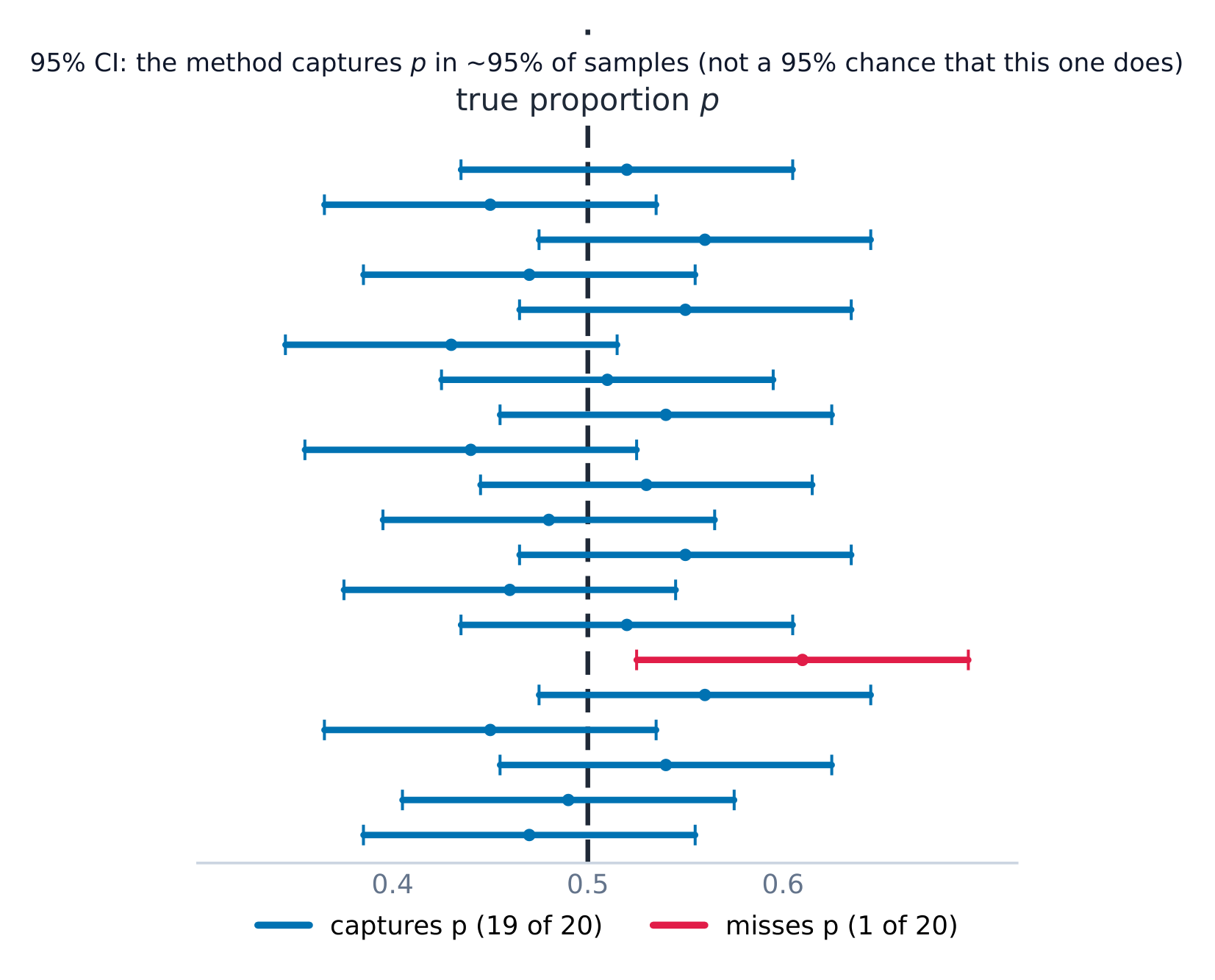
$z^{*}$ is the critical value for the confidence level 置信水平 (e.g. $1.96$ for 95%). Conditions: random sample, Large Counts ($n\hat p\ge 10$ and $n(1-\hat p)\ge 10$), and the 10% condition. Interpret it: "We are 95% confident the true proportion of... is between... and...". Interpret the level: "In 95% of samples, this method produces an interval that captures the true proportion."
Worked example. In a random sample of $200$ people, $120$ support a policy, so $\hat{p}=0.60$. A $95\%$ interval uses $z^*=1.96$:
We are $95\%$ confident the true proportion of supporters is between $53.2\%$ and $66.8\%$.
Choosing the sample size. To keep the margin of error no larger than a target $m$, set $z^{*}\sqrt{\dfrac{\hat p(1-\hat p)}{n}}\le m$ and solve for $n$. When you have no estimate of $\hat p$, use $\hat p=0.5$: it makes $\hat p(1-\hat p)$ as large as possible, giving the safe (largest) required sample size. Always round the result up to the next whole person.
Worked example. How many people must you survey for a $95\%$ interval with margin of error at most $0.03$? Using $\hat p=0.5$ and $z^*=1.96$:
$z^{*}$ — критическое значение для уровня доверия (например, $1.96$ для 95%). Условия: случайная выборка, большие выборки ($n\hat p\ge 10$ и $n(1-\hat p)\ge 10$) и условие 10%. Интерпретация: «Мы уверены на 95%, что истинная доля... находится между... и...». Интерпретация уровня: «В 95% случаев эта методика дает интервал, который захватывает истинную долю».
По множеству выборок примерно 95% доверительных интервалов уровня 95% захватывают истинную долю
Разбор примера. В случайной выборке из $200$ человек $120$ поддерживают политику, поэтому $\hat{p}=0.60$. Доверительный интервал уровня $95\%$ использует $z^*=1.96$:
Мы уверены на $95\%$, что истинная доля сторонников находится между $53.2\%$ и $66.8\%$.
Доверительный интервал уровня 95% охватывает 1,96 стандартных ошибки в каждую сторону от оценки
Выбор размера выборки. Чтобы погрешность не превышала целевого значения $m$, задайте $z^{*}\sqrt{\dfrac{\hat p(1-\hat p)}{n}}\le m$ и решите уравнение относительно $n$. Когда у вас нет оценки для $\hat p$, используйте $\hat p=0.5$: это делает $\hat p(1-\hat p)$ максимально возможным, обеспечивая безопасный (наибольший) требуемый размер выборки. Всегда округляйте результат вверх до целого человека.
Разбор примера. Сколько людей необходимо опросить для получения доверительного интервала уровня $95\%$ с погрешностью не более $0.03$? Используя $\hat p=0.5$ и $z^*=1.96$:
Justifying a Claim from an Interval · Обоснование утверждения по интервалу
Syllabus · Программа
English
Enduring Understanding (UNC-4): An interval of values should be used to estimate parameters, in order to account for uncertainty.
Learning Objective UNC-4.F: Interpret a confidence interval for a population proportion. [Skill 4.B]
UNC-4.F.1 A confidence interval for a population proportion either contains the population proportion or it does not, because each interval is based on random sample data, which varies from sample to sample.
UNC-4.F.2 We are C% confident that the confidence interval for a population proportion captures the population proportion.
UNC-4.F.3 In repeated random sampling with the same sample size, approximately C% of confidence intervals created will capture the population proportion.
UNC-4.F.4 Interpreting a confidence interval for a one-sample proportion should include a reference to the sample taken and details about the population it represents.
Illustrative examples for UNC-4.F.4: For interpreting a 99% confidence interval of (0.268, 0.292), based on the proportion of a nationally representative sample of twelfth-grade students who answered a particular multiple choice question correctly: "We are 99 percent confident that the interval from 0.268 to 0.292 contains the population proportion of all United States twelfth-grade students who would answer this question correctly" (2011 FRQ 6(a)).
Learning Objective UNC-4.G: Justify a claim based on a confidence interval for a population proportion. [Skill 4.D]
UNC-4.G.1 A confidence interval for a population proportion provides an interval of values that may provide sufficient evidence to support a particular claim in context.
Learning Objective UNC-4.H: Identify the relationships between sample size, width of a confidence interval, confidence level, and margin of error for a population proportion. [Skill 4.A]
UNC-4.H.1 When all other things remain the same, the width of the confidence interval for a population proportion tends to decrease as the sample size increases. For a population proportion, the width of the interval is proportional to $\dfrac{1}{\sqrt{n}}$.
UNC-4.H.2 For a given sample, the width of the confidence interval for a population proportion increases as the confidence level increases.
UNC-4.H.3 The width of a confidence interval for a population proportion is exactly twice the margin of error.
Русский
Продолжающееся понимание (UNC-4): Доверительный интервал значений следует использовать для оценки параметров, чтобы учесть неопределенность.
Цель обучения UNC-4.F: Интерпретировать доверительный интервал для доли населения. [Навык 4.B]
UNC-4.F.1 Доверительный интервал для доли населения либо содержит долю населения, либо нет, поскольку каждый интервал основан на данных случайной выборки, которые варьируются от выборки к выборке.
UNC-4.F.2 Мы уверены на C%, что доверительный интервал для доли населения охватывает долю населения.
UNC-4.F.3 При многократном повторении случайной выборки с одинаковым размером выборки приблизительно C% созданных доверительных интервалов будут охватывать долю населения.
UNC-4.F.4 Интерпретация доверительного интервала для одной выборочной доли должна включать ссылку на взятую выборку и детали о представляемой ею генеральной совокупности.
Иллюстративные примеры для UNC-4.F.4: Для интерпретации 99%-го доверительного интервала (0,268; 0,292), основанного на доле учеников двенадцатого класса nationally репрезентативной выборки, ответивших правильно на определенный вопрос с множественным выбором: «Мы уверены на 99 процентов, что интервал от 0,268 до 0,292 содержит долю населения всех учеников двенадцатого класса США, которые ответили бы на этот вопрос правильно» (FRQ 2011, вопрос 6(a)).
Цель обучения UNC-4.G: Обосновать утверждение на основе доверительного интервала для доли населения. [Навык 4.D]
UNC-4.G.1 Доверительный интервал для доли населения предоставляет диапазон значений, который может служить достаточным доказательством для поддержки определенного утверждения в контексте.
Цель обучения UNC-4.H: Выявить взаимосвязи между размером выборки, шириной доверительного интервала, уровнем доверия и погрешностью выборки для доли населения. [Навык 4.A]
UNC-4.H.1 При сохранении остальных условий неизменными ширина доверительного интервала для доли населения имеет тенденцию уменьшаться по мере увеличения размера выборки. Для доли населения ширина интервала пропорциональна $\dfrac{1}{\sqrt{n}}$.
UNC-4.H.2 Для данной выборки ширина доверительного интервала для доли населения увеличивается по мере повышения уровня доверия.
UNC-4.H.3 Ширина доверительного интервала для доли населения точно вдвое больше погрешности выборки.
Source: College Board AP Course and Exam Description · Источник: Описание курса и экзамена College Board AP
English
To judge a claimed value: if it lies inside the interval, the data are consistent with it; if it lies outside, the data give evidence against it. Base the conclusion on whether the plausible values include the claim, in context.
Русский
Чтобы оценить заявленное значение: если оно лежит внутри интервала, данные согласуются с ним; если оно лежит вне интервала, данные свидетельствуют против него. Делайте вывод на основе того, включают ли правдоподобные значения утверждение, в контексте задачи.
6.4
Setting Up a Test for a Proportion · Подготовка теста для доли
Syllabus · Программа
English
Enduring Understanding (VAR-6): The normal distribution may be used to model variation.
Learning Objective VAR-6.D: Identify the null and alternative hypotheses for a population proportion. [Skill 1.F]
VAR-6.D.1 The null hypothesis is the situation that is assumed to be correct unless evidence suggests otherwise, and the alternative hypothesis is the situation for which evidence is being collected.
VAR-6.D.2 For hypotheses about parameters, the null hypothesis contains an equality reference (=, ≥, or ≤), while the alternative hypothesis contains a strict inequality (<, >, or ≠). The type of inequality in the alternative hypothesis is based on the question of interest. Alternative hypotheses with < or > are called one-sided, and alternative hypotheses with ≠ are called two-sided. Although the null hypothesis for a one-sided test may include an inequality symbol, it is still tested at the boundary of equality.
VAR-6.D.3 The null hypothesis for a population proportion is: $H_0 : p = p_0$, where $p_0$ is the null hypothesized value for the population proportion.
VAR-6.D.4 A one-sided alternative hypothesis for a proportion is either $H_a : p < p_0$ or $H_a : p > p_0$. A two-sided alternate hypothesis is $H_a : p_1 \neq p_2$.
VAR-6.D.5 For a one-sample $z$-test for a population proportion, the null hypothesis specifies a value for the population proportion, usually one indicating no difference or effect.
Learning Objective VAR-6.E: Identify an appropriate testing method for a population proportion. [Skill 1.E]
VAR-6.E.1 For a single categorical variable, the appropriate testing method for a population proportion is a one-sample $z$-test for a population proportion.
Learning Objective VAR-6.F: Verify the conditions for making statistical inferences when testing a population proportion. [Skill 4.C]
VAR-6.F.1 In order to make statistical inferences when testing a population proportion, we must check for independence and that the sampling distribution is approximately normal:
a. To check for independence:
i. Data should be collected using a random sample or a randomized experiment.
ii. When sampling without replacement, check that $n \leq 10\%N$.
b. To check that the sampling distribution of $\hat{p}$ is approximately normal (shape):
i. Assuming that $H_0$ is true $(p = p_0)$, verify that both the number of successes, $np_0$, and the number of failures, $n(1-p_0)$ are at least 10 so that that the sample size is large enough to support an assumption of normality.
Русский
Устойчивое понимание (VAR-6): Нормальное распределение может использоваться для моделирования вариации.
Цель обучения VAR-6.D: Определить нулевую и альтернативную гипотезы для доли населения. [Навык 1.F]
VAR-6.D.1 Нулевая гипотеза — это ситуация, которая считается верной, если нет доказательств обратного, а альтернативная гипотеза — это ситуация, для которой собираются доказательства.
VAR-6.D.2 Для гипотез о параметрах нулевая гипотеза содержит ссылку на равенство (=, ≥ или ≤), а альтернативная гипотеза содержит строгое неравенство (<, >, или ≠). Тип неравенства в альтернативной гипотезе определяется интересующим вопросом. Альтернативные гипотезы с < or > называются односторонними, а альтернативные гипотезы с ≠ — двусторонними. Хотя нулевая гипотеза для одностороннего теста может содержать символ неравенства, она все равно проверяется на границе равенства.
VAR-6.D.3 Нулевая гипотеза для доли генеральной совокупности: $H_0 : p = p_0$, где $p_0$ — предполагаемое значение нулевой гипотезы для доли генеральной совокупности.
VAR-6.D.4 Односторонняя альтернативная гипотеза для доли может быть либо $H_a : p < p_0$, либо $H_a : p > p_0$. Двусторонняя альтернативная гипотеза имеет вид $H_a : p_1 \neq p_2$.
VAR-6.D.5 Для одновыборочного z-теста ($z$) для доли генеральной совокупности нулевая гипотеза указывает значение для доли генеральной совокупности, обычно это значение, указывающее на отсутствие различий или эффекта.
Учебная цель VAR-6.E: Определить подходящий метод тестирования для доли генеральной совокупности. [Навык 1.E]
VAR-6.E.1 Для одной категориальной переменной подходящим методом тестирования для доли генеральной совокупности является одновыборочный z-тест ($z$) для доли генеральной совокупности.
Учебная цель VAR-6.F: Проверить условия для проведения статистических выводов при тестировании доли генеральной совокупности. [Навык 4.C]
VAR-6.F.1 Чтобы проводить статистические выводы при тестировании доли генеральной совокупности, необходимо проверить независимость и то, что выборочное распределение приблизительно нормально:
a. Для проверки независимости:
i. Данные следует собирать с использованием случайной выборки или рандомизированного эксперимента.
ii. При выборке без возвращения проверьте, что $n \leq 10\%N$.
b. Для проверки того, что выборочное распределение $\hat{p}$ приближенно нормально (форма):
i. Предполагая, что $H_0$ верно $(p = p_0)$, убедитесь, что как количество успехов, $np_0$, так и количество неудач, $n(1-p_0)$, не менее 10, чтобы размер выборки был достаточно велик для предположения нормальности.
Source: College Board AP Course and Exam Description · Источник: Описание курса и экзамена College Board AP
English
A significance test 显著性检验 weighs evidence against a claim. State a null hypothesis 原假设$H_0$ and an alternative hypothesis 备择假设$H_a$ about the parameter $p$:
Check the same conditions (random, Large Counts using $p_0$, 10%). The test statistic 检验统计量 counts standard errors from $p_0$:
$$z=\frac{\hat p-p_0}{\sqrt{p_0(1-p_0)/n}}.$$
Worked example. A company claims $90\%$ satisfaction ($p_0=0.90$); a sample of $100$ finds $84$ satisfied ($\hat{p}=0.84$). Test $H_0:p=0.90$ vs $H_a:p\neq0.90$ at $\alpha=0.05$:
giving a two-tailed $p$-value of about $2(0.023)=0.046$. Since $0.046<0.05$, reject $H_0$ – there is evidence the true satisfaction rate differs from (is below) $90\%$.
Русский
Тест значимости оценивает доказательства против утверждения. Сформулируйте нулевую гипотезу$H_0$ и альтернативную гипотезу$H_a$ относительно параметра $p$:
Проверьте те же условия (случайность, большие выборки с использованием $p_0$, 10%). Статистика теста показывает количество стандартных ошибок от $p_0$:
$$z=\frac{\hat p-p_0}{\sqrt{p_0(1-p_0)/n}}.$$
Разбор примера. Компания утверждает $90\%$ удовлетворенности ($p_0=0.90$); в выборке из $100$ обнаружено $84$ удовлетворенных ($\hat{p}=0.84$). Проверьте $H_0:p=0.90$ против $H_a:p\neq0.90$ на уровне $\alpha=0.05$:
что дает двустороннее $p$-значение примерно равное $2(0.023)=0.046$. Поскольку $0.046<0.05$, отвергаем $H_0$ – есть доказательства того, что истинная доля удовлетворенных отличается от (ниже) $90\%$.
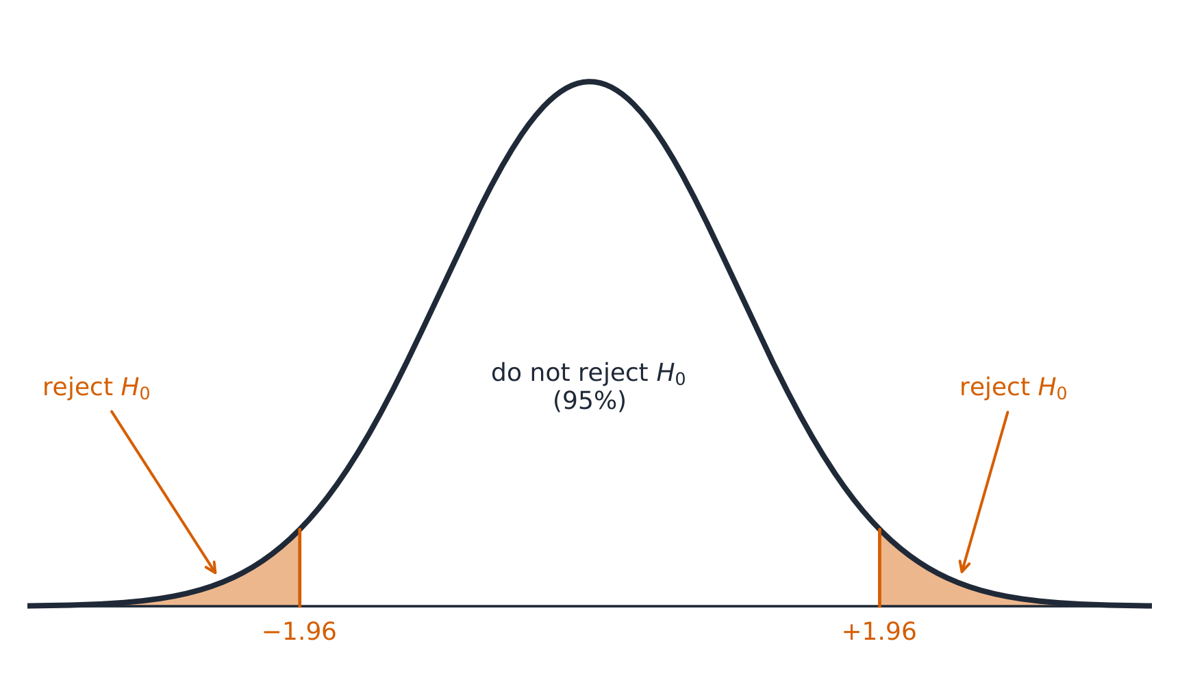
Двусторонний тест на уровне 5% отвергает нулевую гипотезу в заштрихованных хвостах
Enduring Understanding (VAR-6): The normal distribution may be used to model variation.
Learning Objective VAR-6.G: Calculate an appropriate test statistic and $p$-value for a population proportion. [Skill 3.E]
VAR-6.G.1 The distribution of the test statistic assuming the null hypothesis is true (null distribution) can be either a randomization distribution or when a probability model is assumed to be true, a theoretical distribution ($z$).
VAR-6.G.2 When using a $z$-test, the standardized test statistic can be written: $\text{test statistic} = \dfrac{\text{sample statistic} - \text{null value of the parameter}}{\text{standard deviation of the statistic}}$. This is called a $z$-statistic for proportions.
VAR-6.G.3 The test statistic for a population proportion is: $z = \dfrac{\hat{p} - p_0}{\sqrt{\dfrac{p_0(1-p_0)}{n}}}$.
Clarifying statement: The formulas for test statistics do not appear explicitly on the AP Statistics Formula Sheet provided with the AP Statistics Exam. However, these formulas do not need to be memorized, as they can be constructed based on the general test statistic formula and the relevant standard error formulas that are provided on the formula sheet.
VAR-6.G.4 A $p$-value is the probability of obtaining a test statistic as extreme or more extreme than the observed test statistic when the null hypothesis and probability model are assumed to be true. The significance level may be given or determined by the researcher.
Enduring Understanding (DAT-3): Significance testing allows us to make decisions about hypotheses within a particular context.
Learning Objective DAT-3.A: Interpret the $p$-value of a significance test for a population proportion. [Skill 4.B]
DAT-3.A.1 The $p$-value is the proportion of values for the null distribution that are as extreme or more extreme than the observed value of the test statistic. This is:
a. The proportion at or above the observed value of the test statistic, if the alternative is >.
b. The proportion at or below the observed value of the test statistic, if the alternative is <.
c. The proportion less than or equal to the negative of the absolute value of the test statistic plus the proportion greater than or equal to the absolute value of the test statistic, if the alternative is ≠.
DAT-3.A.2 An interpretation of the $p$-value of a significance test for a one-sample proportion should recognize that the $p$-value is computed by assuming that the probability model and null hypothesis are true, i.e., by assuming that the true population proportion is equal to the particular value stated in the null hypothesis.
Русский
Устойчивое понимание (VAR-6): Нормальное распределение может использоваться для моделирования вариации.
Цель обучения VAR-6.G: Вычислить соответствующую тестовую статистику и p-значение ($p$) для доли генеральной совокупности. [Навык 3.E]
VAR-6.G.1 Распределение тестовой статистики при условии истинности нулевой гипотезы (нулевое распределение) может быть либо распределением рандомизации, либо теоретическим распределением ($z$), когда предполагается истинность вероятностной модели.
VAR-6.G.2 При использовании z-теста ($z$) стандартизированная тестовая статистика может быть записана как: $\text{test statistic} = \dfrac{\text{sample statistic} - \text{null value of the parameter}}{\text{standard deviation of the statistic}}$. Это называется z-статистикой ($z$) для долей.
Уточнение: Формулы для тестовых статистик не приводятся явно в Таблице формул AP Statistics, прилагаемой к экзамену по статистике AP. Однако эти формулы не нужно учить наизусть, так как их можно вывести, используя общую формулу тестовой статистики и соответствующие формулы стандартных ошибок, приведенные в таблице формул.
VAR-6.G.4 p-значение ($p$) — это вероятность получения тестовой статистики, такой же экстремальной или более экстремальной, чем наблюдаемая тестовая статистика, при предположении истинности нулевой гипотезы и вероятностной модели. Уровень значимости может быть задан или определен исследователем.
Продолжающееся понимание (DAT-3): Тестирование значимости позволяет нам принимать решения относительно гипотез в конкретном контексте.
Цель обучения DAT-3.A: Интерпретировать p-значение ($p$) значимости теста для доли генеральной совокупности. [Навык 4.B]
DAT-3.A.1 p-значение ($p$) — это доля значений распределения нулевой гипотезы, которые являются такими же экстремальными или более экстремальными, чем наблюдаемое значение тестовой статистики. Это:
a. Доля значений, равных или больших наблюдаемого значения тестовой статистики, если альтернативная гипотеза >.
b. Доля значений, равных или меньших наблюдаемого значения тестовой статистики, если альтернативная гипотеза <.
c. Доля значений, меньших или равных отрицательному значению абсолютной величины тестовой статистики, плюс доля значений, больших или равных абсолютной величине тестовой статистики, если альтернативная гипотеза ≠.
DAT-3.A.2 Интерпретация p-значения ($p$) значимости теста для одновыборочной доли должна учитывать, что это p-значение ($p$) вычисляется при предположении истинности вероятностной модели и нулевой гипотезы, т. е. при предположении, что истинная доля генеральной совокупности равна конкретному значению, указанному в нулевой гипотезе.
Source: College Board AP Course and Exam Description · Источник: Описание курса и экзамена College Board AP
English
What a p-value means
The $p$-value P值 is the probability of getting a sample result as extreme or more extreme than the observed one, assuming $H_0$ is true. A small $p$-value means the data would be surprising if $H_0$ held – evidence against $H_0$. It is not the probability that $H_0$ is true.
Русский
Что означает p-значение
$p$-значение P — это вероятность получить результат выборки такой же экстремальный или более экстремальный, чем наблюдаемый, при условии, что $H_0$ истинно. Малое $p$-значение означает, что данные были бы неожиданными, если бы выполнялось $H_0$ – доказательство против $H_0$. Это не вероятность того, что $H_0$ истинна.
Explore · Исследовать
A p-value as a tail area · p-значение как площадь хвоста
A p-value is the probability, if the null hypothesis were true, of a result at least this extreme — the shaded tail area. Small p-values cast doubt on the null. · p-значение — это вероятность получения результата не менее экстремального, чем данный, при условии истинности нулевой гипотезы; заштрихованная площадь хвоста. Малые p-значения поставляют под сомнение нулевую гипотезу.
6.6
Concluding a Test · Завершение теста
Syllabus · Программа
Enduring Understanding
Learning Objective
Essential Knowledge
DAT-3
Significance testing allows us to make decisions about hypotheses within a particular context.
DAT-3.B
Justify a claim about the population based on the results of a significance test for a population proportion. [Skill 4.E]
DAT-3.B.1 The significance level, $\alpha$, is the predetermined probability of rejecting the null hypothesis given that it is true.
DAT-3.B.2 A formal decision explicitly compares the $p$-value to the significance level, $\alpha$. If the $p$-value $\leq \alpha$, reject the null hypothesis. If the $p$-value $> \alpha$, fail to reject the null hypothesis.
DAT-3.B.3 Rejecting the null hypothesis means there is sufficient statistical evidence to support the alternative hypothesis. Failing to reject the null means there is insufficient statistical evidence to support the alternative hypothesis.
DAT-3.B.4 The conclusion about the alternative hypothesis must be stated in context.
DAT-3.B.5 A significance test can lead to rejecting or not rejecting the null hypothesis, but can never lead to concluding or proving that the null hypothesis is true. Lack of statistical evidence for the alternative hypothesis is not the same as evidence for the null hypothesis.
DAT-3.B.6 Small $p$-values indicate that the observed value of the test statistic would be unusual if the null hypothesis and probability model were true, and so provide evidence for the alternative. The lower the $p$-value, the more convincing the statistical evidence for the alternative hypothesis.
DAT-3.B.7$p$-values that are not small indicate that the observed value of the test statistic would not be unusual if the null hypothesis and probability model were true, so do not provide convincing statistical evidence for the alternative hypothesis nor do they provide evidence that the null hypothesis is true.
DAT-3.B.8 A formal decision explicitly compares the $p$-value to the significance $\alpha$. If the $p$-value $\leq \alpha$, then reject the null hypothesis, $H_0 : p = p_0$. If the $p$-value $> \alpha$, then fail to reject the null hypothesis.
DAT-3.B.9 The results of a significance test for a population proportion can serve as the statistical reasoning to support the answer to a research question about the population that was sampled.
Source: College Board AP Course and Exam Description · Источник: Описание курса и экзамена College Board AP
English
Compare the $p$-value to the significance level 显著性水平$\alpha$ (often $0.05$):
$p\le\alpha$: reject $H_0$ – there is convincing evidence for $H_a$.
$p>\alpha$: fail to reject $H_0$ – not enough evidence for $H_a$ (never "accept $H_0$").
Always write the conclusion in context, linking back to the claim.
Русский
Сравните значение $p$ со уровнем значимости$\alpha$ (часто $0.05$):
$p\le\alpha$: отвергаем $H_0$ – есть убедительные доказательства в пользу $H_a$.
$p>\alpha$: не отвергаем $H_0$ – недостаточно доказательств для $H_a$ (никогда не «принимаем $H_0$»).
Всегда формулируйте вывод в контексте задачи, связывая его с утверждением.
6.7
Type I and Type II Errors · Ошибки первого и второго рода
Syllabus · Программа
English
Enduring Understanding (UNC-5): Probabilities of Type I and Type II errors influence inference.
Learning Objective UNC-5.A: Identify Type I and Type II errors. [Skill 1.B]
UNC-5.A.1 A Type I error occurs when the null hypothesis is true and is rejected (false positive).
UNC-5.A.2 A Type II error occurs when the null hypothesis is false and is not rejected (false negative).
Table of Errors: With Actual Population Value across the top ($H_0$ true; $H_a$ true) and Decision down the side (Reject $H_0$; Fail to Reject $H_0$): Reject $H_0$ when $H_0$ true = Type I Error; Reject $H_0$ when $H_a$ true = Correct Decision; Fail to Reject $H_0$ when $H_0$ true = Correct Decision; Fail to Reject $H_0$ when $H_a$ true = Type II Error.
Learning Objective UNC-5.B: Calculate the probability of a Type I and Type II errors. [Skill 3.A]
UNC-5.B.1 The significance level, $\alpha$, is the probability of making a Type I error, if the null hypothesis is true.
UNC-5.B.2 The power of a test is the probability that a test will correctly reject a false null hypothesis.
UNC-5.B.3 The probability of making a Type II error $= 1 - power$.
Learning Objective UNC-5.C: Identify factors that affect the probability of errors in significance testing. [Skill 4.A]
UNC-5.C.1 The probability of a Type II error decreases when any of the following occurs, provided the others do not change:
i. Sample size(s) increases.
ii. Significance level ($\alpha$) of a test increases.
iii. Standard error decreases.
iv. True parameter value is farther from the null.
Learning Objective UNC-5.D: Interpret Type I and Type II errors. [Skill 4.B]
UNC-5.D.1 Whether a Type I or a Type II error is more consequential depends upon the situation.
UNC-5.D.2 Since the significance level, $\alpha$, is the probability of a Type I error, the consequences of a Type I error influence decisions about a significance level.
Русский
Принцип устойчивого понимания (UNC-5): Вероятности ошибок I и II рода влияют на выводы.
Обучающая цель UNC-5.A: Определять ошибки I и II рода. [Навык 1.B]
UNC-5.A.1 Ошибка I рода возникает, когда нулевая гипотеза верна, но отвергается (ложноположительный результат).
UNC-5.A.2 Ошибка II рода возникает, когда нулевая гипотеза неверна, но не отвергается (ложноотрицательный результат).
Таблица ошибок: Истинное значение параметра генеральной совокупности — по горизонтали ($H_0$ верно; $H_a$ верно) и Решение — по вертикали (Отвергнуть $H_0$; Не отвергать $H_0$): Отвергнуть $H_0$, когда $H_0$ верно = Ошибка I рода; Отвергнуть $H_0$, когда $H_a$ верно = Правильное решение; Не отвергать $H_0$, когда $H_0$ верно = Правильное решение; Не отвергать $H_0$, когда $H_a$ верно = Ошибка II рода.
Обучающая цель UNC-5.B: Вычислять вероятность ошибки I и II рода. [Навык 3.A]
UNC-5.B.1 Уровень значимости, $\alpha$, является вероятностью совершения ошибки I рода, если нулевая гипотеза верна.
UNC-5.B.2 Мощность теста — это вероятность того, что тест правильно отвергнет неверную нулевую гипотезу.
UNC-5.B.3 Вероятность совершения ошибки II рода = $= 1 - power$.
Обучающая цель UNC-5.C: Определять факторы, влияющие на вероятность ошибок при тестировании значимости. [Навык 4.A]
UNC-5.C.1 Вероятность ошибки II рода уменьшается, когда происходит любое из следующего, при условии, что остальные остаются неизменными:
i. Увеличивается размер(ы) выборки.
ii. Увеличивается уровень значимости ($\alpha$) теста.
iii. Уменьшается стандартная ошибка.
iv. Истинное значение параметра находится дальше от нулевого.
Обучающая цель UNC-5.D: Интерпретировать ошибки I и II рода. [Навык 4.B]
UNC-5.D.1 То, какая ошибка — I или II рода — более серьезна, зависит от конкретной ситуации.
UNC-5.D.2 Поскольку уровень значимости, $\alpha$, является вероятностью ошибки I рода, последствия ошибки I рода влияют на решения относительно уровня значимости.
Source: College Board AP Course and Exam Description · Источник: Описание курса и экзамена College Board AP
English
Type I and Type II errors
A Type I error 第一类错误: rejecting a true$H_0$ (a false alarm). Its probability is $\alpha$.
A Type II error 第二类错误: failing to reject a false$H_0$ (a missed detection). Its probability is $\beta$.
The power 检验效能$=1-\beta$ is the chance of correctly detecting a real effect. Power rises with a larger sample, a larger effect, or a larger $\alpha$.
Describe each error and its consequence in the problem's context.
Русский
Ошибки первого и второго рода
Ошибка I рода: отвержение истинной$H_0$ (ложная тревога). Вероятность этого составляет $\alpha$.
Ошибка II рода: невыполнение отвержения ложной$H_0$ (пропущенное обнаружение). Вероятность этого составляет $\beta$.
Мощность$=1-\beta$ — это вероятность правильно обнаружить реальный эффект. Мощность увеличивается при увеличении объема выборки, размера эффекта или уровня $\alpha$.
Опишите каждую ошибку и её последствия в контексте задачи.
Explore · Исследовать
Two ways a test can be wrong · Два способа ошибки теста
A Type I error rejects a true null (false alarm); a Type II error keeps a false null (a miss). Lowering one usually raises the other. · Ошибка первого рода отвергает истинную нулевую гипотезу (ложная тревога); ошибка второго рода сохраняет ложную нулевую гипотезу (пропуск). Снижение одной обычно повышает другую.
6.8
Confidence Interval for a Difference of Proportions · Доверительный интервал для разности долей
Syllabus · Программа
Enduring Understanding
Learning Objective
Essential Knowledge
UNC-4
An interval of values should be used to estimate parameters, in order to account for uncertainty.
UNC-4.I
Identify an appropriate confidence interval procedure for a comparison of population proportions. [Skill 1.D]
UNC-4.I.1 The appropriate confidence interval procedure for a two-sample comparison of proportions for one categorical variable is a two-sample $z$-interval for a difference between population proportions.
UNC-4.J
Verify the conditions for calculating confidence intervals for a difference between population proportions. [Skill 4.C]
UNC-4.J.1 In order to calculate confidence intervals to estimate a difference between proportions, we must check for independence and that the sampling distribution is approximately normal:
a. To check for independence:
i. Data should be collected using two independent, random samples or a randomized experiment.
ii. When sampling without replacement, check that $n_1 \leq 10\%N_1$ and $n_2 \leq 10\%N_2$.
b. To check that sampling distribution of $\hat{p}_1 - \hat{p}_2$ is approximately normal (shape).
i. For categorical variables, check that $n_1\hat{p}_1$, $n_1(1-\hat{p}_1)$, $n_2\hat{p}_2$, and $n_2\left(1-\hat{p}_2\right)$ are all greater than or equal to some predetermined value, typically either 5 or 10.
UNC-4.K
Calculate an appropriate confidence interval for a comparison of population proportions. [Skill 3.D]
UNC-4.K.1 For a comparison of proportions, the interval estimate is $(\hat{p}_1 - \hat{p}_2) \pm z^* \sqrt{\dfrac{\hat{p}_1(1-\hat{p}_1)}{n_1} + \dfrac{\hat{p}_2(1-\hat{p}_2)}{n_2}}$.
Clarifying statement: Formulas for interval estimates do not appear explicitly on the AP Statistics Formula Sheet provided with the AP Statistics Exam. However, these formulas do not need to be memorized, as they can be constructed based on the general test statistic formula and the relevant standard error formulas that are provided on the formula sheet.
UNC-4.L
Calculate an interval estimate based on a confidence interval for a difference of proportions. [Skill 3.D]
UNC-4.L.1 Confidence intervals for a difference in proportions can be used to calculate interval estimates with specified units.
Source: College Board AP Course and Exam Description · Источник: Описание курса и экзамена College Board AP
Условия должны выполняться в обоих выборках, а сами выборки должны быть независимыми.
6.9
Justifying a Claim About Two Proportions · Обоснование утверждения о двух долях
Syllabus · Программа
Enduring Understanding
Learning Objective
Essential Knowledge
UNC-4
An interval of values should be used to estimate parameters, in order to account for uncertainty.
UNC-4.M
Interpret a confidence interval for a difference of proportions. [Skill 4.B]
UNC-4.M.1 In repeated random sampling with the same sample size, approximately C% of confidence intervals created will capture the difference in population proportions.
UNC-4.M.2 Interpreting a confidence interval for difference between population proportions should include a reference to the sample taken and details about the population it represents.
UNC-4.N
Justify a claim based on a confidence interval for a difference of proportions. [Skill 4.D]
UNC-4.N.1 A confidence interval for difference in population proportions provides an interval of values that may provide sufficient evidence to support a particular claim in context.
Source: College Board AP Course and Exam Description · Источник: Описание курса и экзамена College Board AP
English
If the interval for $p_1-p_2$ contains $0$, the data are consistent with no difference; if it lies entirely above or below $0$, there is evidence of a difference (in that direction). State the direction and context.
Русский
Если интервал для $p_1-p_2$ содержит $0$, данные согласуются с отсутствием различий; если он полностью расположен выше или ниже $0$, есть доказательства различия (в этом направлении). Укажите направление и контекст.
6.10
Setting Up a Test for a Difference · Настройка теста для разности
Syllabus · Программа
English
Enduring Understanding (VAR-6): The normal distribution may be used to model variation.
Learning Objective VAR-6.H: Identify the null and alternative hypotheses for a difference of two population proportions. [Skill 1.F]
VAR-6.H.1 For a two-sample test for a difference of two proportions, the null hypothesis specifies a value of $0$ for the difference in population proportions, indicating no difference or effect.
VAR-6.H.2 The null hypothesis for a difference in proportions is: $H_0 : p_1 = p_2$, or $H_0 : p_1 - p_2 = 0$.
VAR-6.H.3 A one-sided alternative hypothesis for a difference in proportions is $H_a : p_1 < p_2$, or, $H_a : p_1 > p_2$. A two-sided alternative hypothesis for a difference of proportions is $H_a : p_1 \neq p_2$.
Learning Objective VAR-6.I: Identify an appropriate testing method for the difference of two population proportions. [Skill 1.E]
VAR-6.I.1 For a single categorical variable, the appropriate testing method for the difference of two population proportions is a two-sample $z$-test for a difference between two population proportions.
Learning Objective VAR-6.J: Verify the conditions for making statistical inferences when testing a difference of two population proportions. [Skill 4.C]
VAR-6.J.1 In order to make statistical inferences when testing a difference between population proportions, we must check for independence and that the sampling distribution is approximately normal:
a. To check for independence:
i. Data should be collected using two independent, random samples or a randomized experiment.
ii. When sampling without replacement, check that $n_1 \leq 10\%N_1$ and $n_2 \leq 10\%N_2$.
b. To check that the sampling distribution of $\hat{p}_1 - \hat{p}_2$ is approximately normal (shape):
i. For the combined sample, define the combined (or pooled) proportion, $\hat{p}_c = \dfrac{n_1\hat{p}_1 + n_2\hat{p}_2}{n_1 + n_2}$. Assuming that $H_0$ is true $(p_1 - p_2 = 0$ or $p_1 = p_2)$, check that $n_1\hat{p}_c$, $n_1\left(1-\hat{p}_c\right)$, $n_2\hat{p}_c$, and $n_2\left(1-\hat{p}_c\right)$ are all greater than or equal to some predetermined value, typically either 5 or 10.
Русский
Устойчивое понимание (VAR-6): Нормальное распределение может использоваться для моделирования вариации.
Цель обучения VAR-6.H: Определять нулевую и альтернативную гипотезы для разности двух генеральных пропорций. [Навык 1.F]
VAR-6.H.1 Для двухвыборочного теста на разность двух пропорций нулевая гипотеза указывает значение $0$ для разности генеральных пропорций, что означает отсутствие различий или эффекта.
VAR-6.H.2 Нулевая гипотеза для разности пропорций: $H_0 : p_1 = p_2$ или $H_0 : p_1 - p_2 = 0$.
VAR-6.H.3 Односторонняя альтернативная гипотеза для разности пропорций: $H_a : p_1 < p_2$ или, $H_a : p_1 > p_2$. Двусторонняя альтернативная гипотеза для разности пропорций: $H_a : p_1 \neq p_2$.
Цель обучения VAR-6.I: Определить подходящий метод тестирования для разности двух генеральных пропорций. [Навык 1.E]
VAR-6.I.1 Для одной категориальной переменной подходящим методом тестирования для разности двух генеральных пропорций является двухвыборочный $z$-тест для разности двух генеральных пропорций.
Цель обучения VAR-6.J: Проверять условия для проведения статистических выводов при тестировании разности двух генеральных пропорций. [Навык 4.C]
VAR-6.J.1 Чтобы проводить статистические выводы при тестировании разности между генеральными пропорциями, необходимо проверить независимость и近似 нормальность выборочного распределения:
a. Для проверки независимости:
i. Данные должны собираться с помощью двух независимых случайных выборок или рандомизированного эксперимента.
ii. При выборке без возвращения проверьте, что $n_1 \leq 10\%N_1$ и $n_2 \leq 10\%N_2$.
b. Для проверки того, что выборочное распределение $\hat{p}_1 - \hat{p}_2$ приближенно нормально (форма):
i. Для объединенной выборки определите объединенную (или пуловую) пропорцию, $\hat{p}_c = \dfrac{n_1\hat{p}_1 + n_2\hat{p}_2}{n_1 + n_2}$. Предположив, что $H_0$ истинна, проверьте, что $(p_1 - p_2 = 0$ или $p_1 = p_2)$, а также что $n_1\hat{p}_c$, $n_1\left(1-\hat{p}_c\right)$, $n_2\hat{p}_c$ и $n_2\left(1-\hat{p}_c\right)$ все больше или равны некоторому заранее установленному значению, обычно 5 или 10.
Source: College Board AP Course and Exam Description · Источник: Описание курса и экзамена College Board AP
English
Hypotheses compare the two proportions: $H_0: p_1=p_2$ versus $H_a: p_1\neq p_2$ (or $<,>$). Because $H_0$ says the proportions are equal, use a combined (pooled) 合并 sample proportion $\hat p_c=\dfrac{\text{total successes}}{\text{total sample size}}$ to estimate the common $p$.
Русский
Гипотезы сравнивают две доли: $H_0: p_1=p_2$ против $H_a: p_1\neq p_2$ (или $<,>$). Поскольку $H_0$ предполагает равенство долей, используйте совмещенную (pooled) выборочную долю $\hat p_c=\dfrac{\text{total successes}}{\text{total sample size}}$ для оценки общей $p$.
6.11
Carrying Out a Test for a Difference · Проведение теста для разности
Syllabus · Программа
Enduring Understanding
Learning Objective
Essential Knowledge
VAR-6
The normal distribution may be used to model variation.
VAR-6.K
Calculate an appropriate test statistic for the difference of two population proportions. [Skill 3.E]
VAR-6.K.1 The test statistic for a difference in proportions is: $z = \dfrac{(\hat{p}_1 - \hat{p}_2) - 0}{\sqrt{\hat{p}_c(1-\hat{p}_c)}\sqrt{\dfrac{1}{n_1} + \dfrac{1}{n_2}}}$, where $\hat{p}_c = \dfrac{n_1\hat{p}_1 + n_2\hat{p}_2}{n_1 + n_2}$.
Clarifying statement: The formulas for test statistics do not appear explicitly on the AP Statistics Formula Sheet provided with the AP Statistics Exam. However, these formulas do not need to be memorized, as they can be constructed based on the general test statistic formula and the standard error formulas for each of the relevant test statistics that are provided on the formula sheet.
DAT-3
Significance testing allows us to make decisions about hypotheses within a particular context.
DAT-3.C
Interpret the $p$-value of a significance test for a difference of population proportions. [Skill 4.B]
DAT-3.C.1 An interpretation of the $p$-value of a significance test for a difference of two population proportions should recognize that the $p$-value is computed by assuming that the null hypothesis is true, i.e., by assuming that the true population proportions are equal to each other.
DAT-3.D
Justify a claim about the population based on the results of a significance test for a difference of population proportions. [Skill 4.E]
DAT-3.D.1 A formal decision explicitly compares the $p$-value to the significance $\alpha$. If the $p\text{-value} \leq \alpha$, then reject the null hypothesis, $H_0 : p_1 = p_2$, or $H_0 : p_1 - p_2 = 0$. If the $p$-value $> \alpha$, then fail to reject the null hypothesis.
DAT-3.D.2 The results of a significance test for a difference of two population proportions can serve as the statistical reasoning to support the answer to a research question about the two populations that were sampled.
Source: College Board AP Course and Exam Description · Источник: Описание курса и экзамена College Board AP
Найдите $p$-значение из нормального распределения, сравните с $\alpha$ и сделайте вывод в контексте – та же четырехшаговая логика, что и для теста одной доли.
6.11
Exam tips · Советы для экзамена
English
State the conditions (random, 10%, large counts $np,\,nq\ge10$) before any proportion inference.
A confidence interval = estimate $\pm$ margin of error; "95% confident" refers to the method's long-run capture rate.
For a test, write $H_0$ and $H_a$, compute the test statistic, find the p-value, and compare to $\alpha$.
A small p-value is evidence against$H_0$; failing to reject does not prove $H_0$.
Larger samples shrink the margin of error; a higher confidence level widens it.
Русский
Укажите условия (случайная, 10%, большие частоты $np,\,nq\ge10$) перед любым статистическим выводом о доле.
Доверительный интервал = оценка погрешности $\pm$; «95% уверенность» относится к методу его долгосрочной способности захватывать параметр.
Для теста запишите $H_0$ и $H_a$, вычислите тестовую статистику, найдите p-значение и сравните с $\alpha$.
Малое p-значение является доказательством против$H_0$; невыполнение отвержения не доказывает $H_0$.
Большие выборки уменьшают погрешность; более высокий уровень доверия увеличивает её.
Interactive lessons on this topic · Интерактивные уроки по этой теме
Work through it step by step, with instant-check exercises. · Пройдите его шаг за шагом с упражнениями мгновенной проверки.
Pick one and the site follows you — notes, papers, videos and practice all open on it. · Выберите один, и сайт будет вести вас — конспекты, работы, видео и практика откроются там.
Type to search notes, lessons, code, vocabulary and past-paper questions across every subject. · Введите запрос для поиска заметок, уроков, кода, словаря и вопросов с реальных экзаменов по всем предметам.