Skip to content · ⁨Перейти к содержанию⁩
Subjects · ⁨Предметы⁩

AP Statistics

Tips · ⁨Советы⁩

AP Statistics covers exploring data, sampling and experimental design, probability and random variables, sampling distributions, and inference — confidence intervals and significance tests. There is little algebra; the difficulty is saying the right thing about uncertainty.

Every inference answer has four parts: name the procedure, check the conditions, compute, and conclude in context with a link to the alternative hypothesis. The rubric grades all four, so a correct p-value alone scores poorly.

Language is graded. "We reject H₀" is not "we prove H₁"; a confidence interval is about the method's long-run behaviour, not the probability that a particular interval contains the parameter. These distinctions decide marks.

The notes work through all nine units with each inference procedure set out step by step. Released FRQs are in the library. Statistics gives marks for stating the conditions and interpreting in context, so every worked answer names the conditions before it runs the test.

  • 1

    Exploring One-Variable Data · ⁨Исследование данных одной переменной⁩

    Watch lesson · ⁨Смотреть урок⁩
    1.1

    Introducing Statistics: What Can We Learn from Data?

    Syllabus · ⁨Программа⁩
    English

    Enduring Understanding (VAR-1): Given that variation may be random or not, conclusions are uncertain.

    Learning Objective VAR-1.A: Identify questions to be answered, based on variation in one-variable data. [Skill 1.A]

    • VAR-1.A.1 Numbers may convey meaningful information, when placed in context.
    Русский

    Вечная идея (VAR-1): Поскольку вариация может быть случайной или нет, выводы остаются неопределенными.

    Цель обучения VAR-1.A: Сформулировать вопросы для ответа на основе вариации в одномерных данных. [Навык 1.A]

    • VAR-1.A.1 Числа могут передавать значимую информацию, когда помещены в контекст.
    Source: College Board AP Course and Exam Description · ⁨Источник: Описание курса и экзамена College Board AP⁩

    Statistics 统计学 is the science of learning from data 数据 – numbers or labels collected from the real world. Data vary, so we describe patterns and account for the variation 变异 rather than expecting every value to match. A statistical question anticipates an answer based on data that vary.

    Two distinctions run through the whole course. A parameter 参数 is a numerical summary of a whole population; a statistic 统计量 is a numerical summary of a sample - we use the statistic to estimate the parameter we cannot measure directly. And descriptive statistics 描述统计 only summarise the data set in hand, while inferential statistics 推断统计 use a sample to make and test claims about the larger population.

    Vocabulary · ⁨Словарь⁩ Train · ⁨Тренировать⁩
    English Русский
    Statistics/stəˈtɪstɪks/ Статистика
    data/ˈdeɪtə/ данные
    variation/ˌveərɪˈeɪʃn/ вариация
    parameter/pəˈræmɪtə/ параметром
    statistic/stəˈtɪstɪk/ статистикой
    descriptive statistics/dɪˈskrɪptɪv stəˈtɪstɪks/ описательная статистика
    inferential statistics/ɪnfəˈrenʃl stəˈtɪstɪks/ инференциальная статистика
    1.2

    The Language of Variation: Variables

    Syllabus · ⁨Программа⁩
    English

    Enduring Understanding (VAR-1): Given that variation may be random or not, conclusions are uncertain.

    Learning Objective VAR-1.B: Identify variables in a set of data. [Skill 2.A]

    • VAR-1.B.1 A variable is a characteristic that changes from one individual to another.

    Learning Objective VAR-1.C: Classify types of variables. [Skill 2.A]

    • VAR-1.C.1 A categorical variable takes on values that are category names or group labels.
    • VAR-1.C.2 A quantitative variable is one that takes on numerical values for a measured or counted quantity.
      • Illustrative examples for VAR-1.C:
        • Categorical variables:
          • Dominant hand
          • Age group (young or old)
          • Highest degree earned
        • Quantitative variables:
          • Age of a structure
          • Height of a child
          • Concentration of a sample
    Русский

    Вечная идея (VAR-1): Поскольку вариация может быть случайной или нет, выводы остаются неопределенными.

    Цель обучения VAR-1.B: Идентифицировать переменные в наборе данных. [Навык 2.A]

    • VAR-1.B.1 Переменная — это характеристика, которая меняется от одного индивида к другому.

    Цель обучения VAR-1.C: Классифицировать типы переменных. [Навык 2.A]

    • VAR-1.C.1 Категориальная переменная принимает значения, являющиеся названиями категорий или метками групп.
    • VAR-1.C.2 Количественная переменная — это та, которая принимает числовые значения для измеренного или подсчитанного количества.
      • Иллюстративные примеры для VAR-1.C:
        • Категориальные переменные:
          • Доминирующая рука
          • Возрастная группа (молодая или старая)
          • Высшая полученная степень
        • Количественные переменные:
          • Возраст сооружения
          • Рост ребенка
          • Концентрация образца

    Source: College Board AP Course and Exam Description · ⁨Источник: Описание курса и экзамена College Board AP⁩

    A variable 变量 is a characteristic that can differ between individuals. Two kinds:

    • Categorical 分类 (qualitative): values are labels/groups (eye colour, brand).
    • Quantitative 定量: values are numbers you can do arithmetic on (height, age). Quantitative variables are discrete (countable) or continuous (measured).

    Choosing the right graph and summary depends on which kind you have.

    Explore · ⁨Исследовать⁩

    Categorical or quantitative? · ⁨Категориальная или количественная?⁩

    Every variable is either categorical (it labels each unit with a group) or quantitative (a measured number you can average). Which kind it is decides the graphs and summaries you are allowed to use. · ⁨Каждая переменная либо категориальная (она присваивает каждому элементу группу), либо количественная (измеряемое число, которое можно усреднить). То, какой она является, определяет графики и сводки, которые вы можете использовать.⁩

    Vocabulary · ⁨Словарь⁩ Train · ⁨Тренировать⁩
    English Русский
    variable/ˈveərɪəbl/ переменной
    Categorical/ˌkætɪˈɡɒrɪkl/ Категориальная
    Quantitative/ˈkwɒntɪteɪtɪv/ Количественная
    1.3

    Representing a Categorical Variable with Tables

    Syllabus · ⁨Программа⁩
    English

    Enduring Understanding (UNC-1): Graphical representations and statistics allow us to identify and represent key features of data.

    Learning Objective UNC-1.A: Represent categorical data using frequency or relative frequency tables. [Skill 2.B]

    • UNC-1.A.1 A frequency table gives the number of cases falling into each category. A relative frequency table gives the proportion of cases falling into each category.

    Learning Objective UNC-1.B: Describe categorical data represented in frequency or relative tables. [Skill 2.A]

    • UNC-1.B.1 Percentages, relative frequencies, and rates all provide the same information as proportions.
    • UNC-1.B.2 Counts and relative frequencies of categorical data reveal information that can be used to justify claims about the data in context.
    Русский

    Постоянное понимание (UNC-1): Графические представления и статистика позволяют нам выявлять и отображать ключевые особенности данных.

    Цель обучения UNC-1.A: Представлять категориальные данные с помощью таблиц частот или относительных частот. [Навык 2.B]

    • UNC-1.A.1 Таблица частот показывает количество случаев, попадающих в каждую категорию. Таблица относительных частот показывает долю случаев, попадающих в каждую категорию.

    Цель обучения UNC-1.B: Описывать категориальные данные, представленные в таблицах частот или относительных частот. [Навык 2.A]

    • UNC-1.B.1 Проценты, относительные частоты и ставки предоставляют ту же информацию, что и пропорции.
    • UNC-1.B.2 Количество и относительные частоты категориальных данных раскрывают информацию, которая может быть использована для обоснования утверждений о данных в контексте.

    Source: College Board AP Course and Exam Description · ⁨Источник: Описание курса и экзамена College Board AP⁩

    A frequency table 频数表 lists each category's count (frequency); a relative frequency 相对频率 table lists each category's proportion 比例 (count ÷ total). Relative frequencies let you compare groups of different sizes fairly.

    Vocabulary · ⁨Словарь⁩ Train · ⁨Тренировать⁩
    English Русский
    frequency table/ˈfriːkwənsi ˈteɪbl/ таблица частот
    relative frequency/ˈrelətɪv ˈfriːkwənsi/ относительная частота
    proportion/prəˈpɔːʃn/ доли
    1.4

    Representing a Categorical Variable with Graphs

    Syllabus · ⁨Программа⁩
    English

    Enduring Understanding (UNC-1): Graphical representations and statistics allow us to identify and represent key features of data.

    Learning Objective UNC-1.C: Represent categorical data graphically. [Skill 2.B]

    • UNC-1.C.1 Bar charts (or bar graphs) are used to display frequencies (counts) or relative frequencies (proportions) for categorical data.
    • UNC-1.C.2 The height or length of each bar in a bar graph corresponds to either the number or proportion of observations falling within each category.
    • UNC-1.C.3 There are many additional ways to represent frequencies (counts) or relative frequencies (proportions) for categorical data.

    Learning Objective UNC-1.D: Describe categorical data represented graphically. [Skill 2.A]

    • UNC-1.D.1 Graphical representations of a categorical variable reveal information that can be used to justify claims about the data in context.

    Learning Objective UNC-1.E: Compare multiple sets of categorical data. [Skill 2.D]

    • UNC-1.E.1 Frequency tables, bar graphs, or other representations can be used to compare two or more data sets in terms of the same categorical variable.
    Русский

    Постоянное понимание (UNC-1): Графические представления и статистика позволяют нам выявлять и отображать ключевые особенности данных.

    Цель обучения UNC-1.C: Представлять категориальные данные графически. [Навык 2.B]

    • UNC-1.C.1 Столбчатые диаграммы (или гистограммы) используются для отображения частот (количеств) или относительных частот (пропорций) для категориальных данных.
    • UNC-1.C.2 Высота или длина каждого столбца на столбчатой диаграмме соответствует либо количеству, либо доле наблюдений, попадающих в каждую категорию.
    • UNC-1.C.3 Существует множество дополнительных способов представления частот (количеств) или относительных частот (пропорций) для категориальных данных.

    Цель обучения UNC-1.D: Описывать категориальные данные, представленные графически. [Навык 2.A]

    • UNC-1.D.1 Графические представления категориальной переменной раскрывают информацию, которая может быть использована для обоснования утверждений о данных в контексте.

    Цель обучения UNC-1.E: Сравнивать несколько наборов категориальных данных. [Навык 2.D]

    • UNC-1.E.1 Таблицы частот, столбчатые диаграммы или другие представления могут использоваться для сравнения двух или более наборов данных по одной и той же категориальной переменной.

    Source: College Board AP Course and Exam Description · ⁨Источник: Описание курса и экзамена College Board AP⁩

    Bar charts 条形图 show the count or proportion of each category as separated bars; a pie chart shows each category's share of the whole. The bar heights (or slices) let you compare categories at a glance. Bars may be ordered by size or by a natural category order.

    Explore · ⁨Исследовать⁩

    Show a categorical variable as a pie chart · ⁨Покажите категориальную переменную в виде круговой диаграммы⁩

    A pie chart turns each category's share of the whole into a slice: a bigger share is a bigger slice, and every slice together makes 100%. It is a picture of a relative-frequency table. · ⁨Круговая диаграмма превращает долю каждой категории в целое в кусок пирога: большая доля — большой кусок, и все куски вместе составляют 100%. Это изображение таблицы относительной частоты.⁩

    Vocabulary · ⁨Словарь⁩ Train · ⁨Тренировать⁩
    English Русский
    Bar charts/bɑː tʃɑːts/ столбчатые диаграммы
    1.5

    Representing a Quantitative Variable with Graphs

    Syllabus · ⁨Программа⁩
    English

    Enduring Understanding (UNC-1): Graphical representations and statistics allow us to identify and represent key features of data.

    Learning Objective UNC-1.F: Classify types of quantitative variables. [Skill 2.A]

    • UNC-1.F.1 A discrete variable can take on a countable number of values. The number of values may be finite or countably infinite, as with the counting numbers.
    • UNC-1.F.2 A continuous variable can take on infinitely many values, but those values cannot be counted. No matter how small the interval between two values of a continuous variable, it is always possible to determine another value between them.
      • Illustrative examples for UNC-1.F:
        • A discrete variable:
          • Number of students in a class
        • A continuous variable:
          • Height of a child

    Learning Objective UNC-1.G: Represent quantitative data graphically. [Skill 2.B]

    • UNC-1.G.1 In a histogram, the height of each bar shows the number or proportion of observations that fall within the interval corresponding to that bar. Altering the interval widths can change the appearance of the histogram.
    • UNC-1.G.2 In a stem and leaf plot, each data value is split into a "stem" (the first digit or digits) and a "leaf" (usually the last digit).
    • UNC-1.G.3 A dotplot represents each observation by a dot, with the position on the horizontal axis corresponding to the data value of that observation, with nearly identical values stacked on top of each other.
    • UNC-1.G.4 A cumulative graph represents the number or proportion of a data set less than or equal to a given number.
    • UNC-1.G.5 There are many additional ways to graphically represent distributions of quantitative data.
    Русский

    Постоянное понимание (UNC-1): Графические представления и статистика позволяют нам выявлять и отображать ключевые особенности данных.

    Цель обучения UNC-1.F: Классифицировать типы количественных переменных. [Навык 2.A]

    • UNC-1.F.1 Дискретная переменная может принимать конечное или счетно-бесконечное число значений, например, натуральные числа при подсчете.
    • UNC-1.F.2 Непрерывная переменная может принимать бесконечно много значений, но эти значения нельзя пересчитать. Как бы мал ни был интервал между двумя значениями непрерывной переменной, всегда можно определить другое значение между ними.
      • Иллюстративные примеры для UNC-1.F:
        • Дискретная переменная:
          • Количество студентов в классе
        • Непрерывная переменная:
          • Рост ребенка

    Цель обучения UNC-1.G: Представлять количественные данные графически. [Навык 2.B]

    • UNC-1.G.1 На гистограмме высота каждого столбца показывает количество или долю наблюдений, попадающих в интервал, соответствующий этому столбцу. Изменение ширины интервалов может изменить внешний вид гистограммы.
    • UNC-1.G.2 В диаграмме «стебель и листья» каждое значение данных разделяется на «стебель» (первая цифра или цифры) и «лист» (обычно последняя цифра).
    • UNC-1.G.3 Точечная диаграмма представляет каждое наблюдение точкой, положение которой на горизонтальной оси соответствует значению данных этого наблюдения; почти идентичные значения располагаются друг над другом.
    • UNC-1.G.4 Кумулятивный график представляет количество или долю набора данных, меньших или равных заданному числу.
    • UNC-1.G.5 Существует множество дополнительных способов графического представления распределения количественных данных.

    Source: College Board AP Course and Exam Description · ⁨Источник: Описание курса и экзамена College Board AP⁩

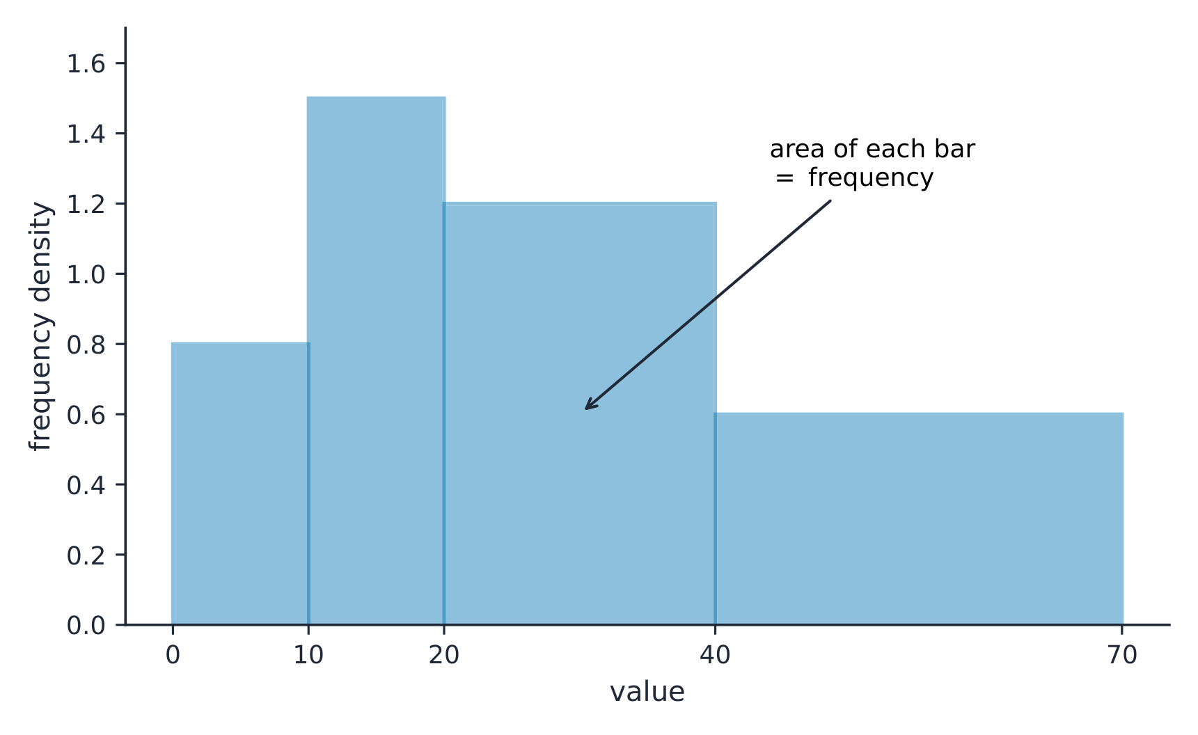
    For numbers, use a dotplot 点图, stem-and-leaf plot 茎叶图, or histogram 直方图 (bars over value intervals called bins). These show the distribution 分布 – how the values spread out. A histogram's bin width changes the picture, so choose it to reveal the shape.

    On a histogram with unequal class widths the bar area is the frequency
    On a histogram with unequal class widths the bar area is the frequency
    Explore · ⁨Исследовать⁩

    Explore how bin width shapes a histogram · ⁨Исследуйте, как ширина интервала формирует гистограмму⁩

    A histogram groups data into equal-width bins and draws a bar over each. Change the bins and notice how the same data can look jagged (too narrow) or smooth (too wide) — the shape is a choice. · ⁨Гистограмма группирует данные в равные интервалы и рисует столбец над каждым. Измените интервалы и заметьте, как одни и те же данные могут выглядеть рваными (слишком узкие) или гладкими (слишком широкие) — форма является выбором.⁩

    Vocabulary · ⁨Словарь⁩ Train · ⁨Тренировать⁩
    English Русский
    dotplot/ˈdɒtplɒt/ точечный график
    stem-and-leaf plot/stem ænd liːf plɒt/ график «стебель-листья»
    histogram/ˈhɪstəɡræm/ гистограмма
    distribution/ˌdɪstrɪˈbjuːʃn/ распределение
    1.6

    Describing the Distribution of a Quantitative Variable

    Syllabus · ⁨Программа⁩
    English

    Enduring Understanding (UNC-1): Graphical representations and statistics allow us to identify and represent key features of data.

    Learning Objective UNC-1.H: Describe the characteristics of quantitative data distributions. [Skill 2.A]

    • UNC-1.H.1 Descriptions of the distribution of quantitative data include shape, center, and variability (spread), as well as any unusual features such as outliers, gaps, clusters, or multiple peaks.
    • UNC-1.H.2 Outliers for one-variable data are data points that are unusually small or large relative to the rest of the data.
    • UNC-1.H.3 A distribution is skewed to the right (positive skew) if the right tail is longer than the left. A distribution is skewed to the left (negative skew) if the left tail is longer than the right. A distribution is symmetric if the left half is the mirror image of the right half.
    • UNC-1.H.4 Univariate graphs with one main peak are known as unimodal. Graphs with two prominent peaks are bimodal. A graph where each bar height is approximately the same (no prominent peaks) is approximately uniform.
    • UNC-1.H.5 A gap is a region of a distribution between two data values where there are no observed data.
    • UNC-1.H.6 Clusters are concentrations of data usually separated by gaps.
    • UNC-1.H.7 Descriptive statistics does not attribute properties of a data set to a larger population, but may provide the basis for conjectures for subsequent testing.
    Русский

    Постоянное понимание (UNC-1): Графические представления и статистика позволяют нам выявлять и отображать ключевые особенности данных.

    Цель обучения UNC-1.H: Описывать характеристики распределений количественных данных. [Навык 2.A]

    • UNC-1.H.1 Описание распределения количественных данных включает форму, центр и изменчивость (разброс), а также любые необычные особенности, такие как выбросы, разрывы, скопления или множественные пики.
    • UNC-1.H.2 Выбросы для одномерных данных — это точки данных, которые являются необычно маленькими или большими по сравнению с остальными данными.
    • UNC-1.H.3 Распределение имеет правый скос (положительный скос), если правый хвост длиннее левого. Распределение имеет левый скос (отрицательный скос), если левый хвост длиннее правого. Распределение является симметричным, если левая половина является зеркальным отражением правой половины.
    • UNC-1.H.4 Одномерные графики с одним основным пиком называются унимодальными. Графики с двумя выраженными пиками — бимодальными. График, где высота каждого столбца примерно одинакова (нет выраженных пиков), называется приблизительно равномерным.
    • UNC-1.H.5 Разрыв — это область распределения между двумя значениями данных, где нет наблюдаемых данных.
    • UNC-1.H.6 Скопления — это концентрации данных, обычно разделенные разрывами.
    • UNC-1.H.7 Описательная статистика не приписывает свойства выборки большей совокупности, но может служить основой для выдвижения гипотез для последующей проверки.

    Source: College Board AP Course and Exam Description · ⁨Источник: Описание курса и экзамена College Board AP⁩

    Describe four things (remember SOCS):

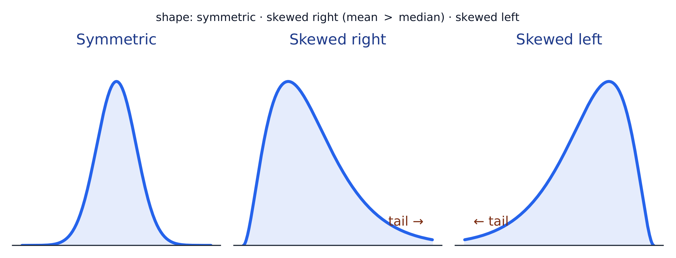
    • Shape 形状: symmetric, or skewed 偏斜 left/right (a long tail on that side), and how many peaks - one main peak is unimodal 单峰, two prominent peaks bimodal 双峰, and roughly equal bars uniform 均匀.
    • Outliers 离群值: unusual values far from the rest.
    • Center: a typical value (mean or median).
    • Spread: how much the values vary (range, IQR, standard deviation).

    Always describe shape/center/spread in context, with units.

    The shape of a distribution: symmetric, skewed right (long right tail), or skewed left
    The shape of a distribution: symmetric, skewed right (long right tail), or skewed left
    Vocabulary · ⁨Словарь⁩ Train · ⁨Тренировать⁩
    English Русский
    Shape/ʃeɪp/ Фигура
    skewed/skjuːd/ асимметричное
    unimodal/ˌʌnɪˈmɒdl/ унимодальный
    bimodal/baɪˈmɒdl/ бимодальный
    uniform/ˈjuːnɪfɔːm/ однородное
    Outliers/ˈaʊtlaɪəz/ выбросы (outliers)
    1.7

    Summary Statistics for a Quantitative Variable

    Syllabus · ⁨Программа⁩
    Enduring UnderstandingLearning ObjectiveEssential Knowledge

    UNC-1
    Graphical representations and statistics allow us to identify and represent key features of data.

    UNC-1.I
    Calculate measures of center and position for quantitative data. [Skill 2.C]

    • UNC-1.I.1 A statistic is a numerical summary of sample data.
    • UNC-1.I.2 The mean is the sum of all the data values divided by the number of values. For a sample, the mean is denoted by $x$-bar: $\bar{x} = \dfrac{1}{n}\sum_{i=1}^{n} x_i$, where $x_i$ represents the $i^{\text{th}}$ data point in the sample and $n$ represents the number of data values in the sample.
    • UNC-1.I.3 The median of a data set is the middle value when data are ordered. When the number of data points is even, the median can take on any value between the two middle values. In AP Statistics, the most commonly used value for the median of a data set with an even number of values is the average of the two middle values.
    • UNC-1.I.4 The first quartile, Q1, is the median of the half of the ordered data set from the minimum to the position of the median. The third quartile, Q3, is the median of the half of the ordered data set from the position of the median to the maximum. Q1 and Q3 form the boundaries for the middle 50% of values in an ordered data set.
    • UNC-1.I.5 The $p^{\text{th}}$ percentile is interpreted as the value that has $p\%$ of the data less than or equal to it.

    UNC-1.J
    Calculate measures of variability for quantitative data. [Skill 2.C]

    • UNC-1.J.1 Three commonly used measures of variability (or spread) in a distribution are the range, interquartile range, and standard deviation.
    • UNC-1.J.2 The range is defined as the difference between the maximum data value and the minimum data value. The interquartile range (IQR) is defined as the difference between the third and first quartiles: $Q3 - Q1$. Both the range and the interquartile range are possible ways of measuring variability of the distribution of a quantitative variable.
    • UNC-1.J.3 Standard deviation is a way to measure variability of the distribution of a quantitative variable. For a sample, the standard deviation is denoted by $s$: $s_x = \sqrt{\dfrac{1}{n-1}\sum(x_i - \bar{x})^2}$. The square of the sample standard deviation, $s^2$, is called the sample variance.
    • UNC-1.J.4 Changing units of measurement affects the values of the calculated statistics.

    UNC-1.K
    Explain the selection of a particular measure of center and/or variability for describing a set of quantitative data. [Skill 4.B]

    • UNC-1.K.1 There are many methods for determining outliers. Two methods frequently used in this course are:
      • UNC-1.K.1.i An outlier is a value greater than $1.5 \times \text{IQR}$ above the third quartile or more than $1.5 \times \text{IQR}$ below the first quartile.
      • UNC-1.K.1.ii An outlier is a value located 2 or more standard deviations above, or below, the mean.
    • UNC-1.K.2 The mean, standard deviation, and range are considered nonresistant (or non-robust) because they are influenced by outliers. The median and IQR are considered resistant (or robust), because outliers do not greatly (if at all) affect their value.

    Source: College Board AP Course and Exam Description · ⁨Источник: Описание курса и экзамена College Board AP⁩

    Standard deviation: spread about the mean
    • Center: the mean 均值 $\bar{x}=\dfrac{\sum x_i}{n}$ (average) and the median 中位数 (middle value). The median resists outliers; the mean is pulled toward a skew.
    • Spread: the range, the interquartile range 四分位距 $\text{IQR}=Q_3-Q_1$ (middle 50%), and the standard deviation 标准差 $s_x=\sqrt{\dfrac{\sum(x_i-\bar{x})^2}{n-1}}$ (typical distance from the mean; its square is the variance 方差).
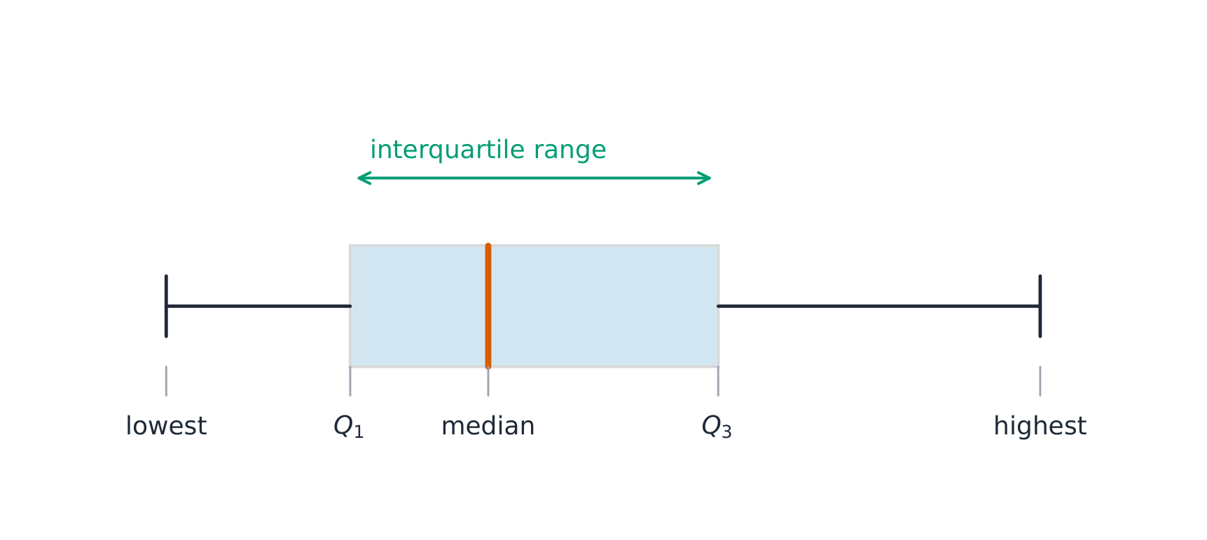
    • The five-number summary 五数概括: min, $Q_1$, median, $Q_3$, max.

    Use resistant measures (median, IQR) for skewed data; mean and standard deviation for roughly symmetric data.

    The percentile 百分位数 of a value is the percent of the data at or below it – so the median is the 50th percentile and $Q_1$ the 25th. A cumulative relative frequency graph 累积相对频率图 makes percentiles easy to read: for each value it plots the proportion of the data at or below it, rising from 0 to 1. Go up from a value to the curve and across to its percentile, or reverse the steps to find the value at a given percentile (the same reading works from a cumulative-frequency table).

    Worked example. For the data $4, 8, 6, 10, 7$: the mean is $\bar{x}=\dfrac{4+8+6+10+7}{5}=\dfrac{35}{5}=7$. Sorting to $4,6,7,8,10$, the median is the middle value, $7$. The mean and median agree here because the data are roughly symmetric.

    Vocabulary · ⁨Словарь⁩ Train · ⁨Тренировать⁩
    English Русский
    mean/miːn/ среднее значение
    median/ˈmiːdiːən/ медианой
    interquartile range/ˌɪntəˈkwɔːtaɪl reɪndʒ/ межквартильный размах
    standard deviation/ˈstændəd ˌdiːvɪˈeɪʃn/ стандартное отклонение
    variance/ˈveərɪəns/ дисперсией
    five-number summary/faɪv ˈnʌmbə ˈsʌməri/ пятизначной сводки
    percentile/pəˈsentaɪl/ перцентиль
    cumulative relative frequency graph/ˈkjuːmjʊlətɪv ˈrelətɪv ˈfriːkwənsi ɡræf/ график кумулятивной относительной частоты
    1.8

    Graphical Representations of Summary Statistics

    Syllabus · ⁨Программа⁩
    English

    Enduring Understanding (UNC-1): Graphical representations and statistics allow us to identify and represent key features of data.

    Learning Objective UNC-1.L: Represent summary statistics for quantitative data graphically. [Skill 2.B]

    • UNC-1.L.1 Taken together, the minimum data value, the first quartile (Q1), the median, the third quartile (Q3), and the maximum data value make up the five-number summary.
    • UNC-1.L.2 A boxplot is a graphical representation of the five-number summary (minimum, first quartile, median, third quartile, maximum). The box represents the middle 50% of data, with a line at the median and the ends of the box corresponding to the quartiles. Lines ("whiskers") extend from the quartiles to the most extreme point that is not an outlier, and outliers are indicated by their own symbol beyond this.

    Learning Objective UNC-1.M: Describe summary statistics of quantitative data represented graphically. [Skill 2.A]

    • UNC-1.M.1 Summary statistics of quantitative data, or of sets of quantitative data, can be used to justify claims about the data in context.
    • UNC-1.M.2 If a distribution is relatively symmetric, then the mean and median are relatively close to one another. If a distribution is skewed right, then the mean is usually to the right of the median. If the distribution is skewed left, then the mean is usually to the left of the median.
    Русский

    Постоянное понимание (UNC-1): Графические представления и статистика позволяют нам выявлять и отображать ключевые особенности данных.

    Учебная цель UNC-1.L: Графически представлять сводную статистику для количественных данных. [Навык 2.B]

    • UNC-1.L.1 Совокупность минимального значения данных, первого квартиля (Q1), медианы, третьего квартиля (Q3) и максимального значения данных составляет пятичисловую сводку.
    • UNC-1.L.2 Ящик с усами — это графическое представление пятичисловой сводки (минимум, первый квартиль, медиана, третий квартиль, максимум). Ящик представляет средние 50% данных, линия проходит через медиану, а концы ящика соответствуют квартилям. Линии («усы») тянутся от квартилей к наиболее экстремальной точке, которая не является выбросом, а выбросы обозначаются собственным символом за пределами этого диапазона.

    Учебная цель UNC-1.M: Описывать сводную статистику количественных данных, представленную графически. [Навык 2.A]

    • UNC-1.M.1 Сводная статистика количественных данных или наборов количественных данных может использоваться для обоснования утверждений о данных в контексте.
    • UNC-1.M.2 Если распределение относительно симметрично, то среднее и медиана находятся относительно близко друг к другу. Если распределение скошено вправо, то среднее обычно находится правее медианы. Если распределение скошено влево, то среднее обычно находится левее медианы.

    Source: College Board AP Course and Exam Description · ⁨Источник: Описание курса и экзамена College Board AP⁩

    A boxplot 箱线图 draws the five-number summary: a box from $Q_1$ to $Q_3$ with the median inside, and whiskers to the most extreme non-outlier values. A point is an outlier if it lies more than $1.5\times\text{IQR}$ beyond a quartile – a rule you may be asked to apply. Boxplots are ideal for comparing several groups side by side.

    Worked example. A dataset has $Q_1=20$ and $Q_3=32$, so $\text{IQR}=12$. The outlier fences are $Q_1-1.5(12)=2$ and $Q_3+1.5(12)=50$. Any value below $2$ or above $50$ is flagged as an outlier.

    A box-and-whisker plot shows the quartiles and the range
    A box-and-whisker plot shows the quartiles and the range
    A boxplot draws the five-number summary; the box spans the IQR
    A boxplot draws the five-number summary; the box spans the IQR
    Explore · ⁨Исследовать⁩

    Explore the five-number summary as a boxplot · ⁨Исследуйте пятичисловое описание как точечный график⁩

    Drag $Q_1$, the median, and $Q_3$ to see the box (its length is the IQR) and how the median's position inside the box reveals skew — a median close to $Q_1$ signals a right-skewed distribution. · ⁨Перетащите $Q_1$, медиану, и $Q_3$, чтобы увидеть коробку (её длина — IQR) и то, как положение медианы внутри коробки раскрывает асимметрию — медиана, близкая к $Q_1$, сигнализирует о правосторонней асимметрии распределения.⁩

    Vocabulary · ⁨Словарь⁩ Train · ⁨Тренировать⁩
    English Русский
    boxplot/ˈbɒksplɒt/ ящик с усами (бокс-плот)
    1.9

    Comparing Distributions of a Quantitative Variable

    Syllabus · ⁨Программа⁩
    English

    Enduring Understanding (UNC-1): Graphical representations and statistics allow us to identify and represent key features of data.

    Learning Objective UNC-1.N: Compare graphical representations for multiple sets of quantitative data. [Skill 2.D]

    • UNC-1.N.1 Any of the graphical representations, e.g., histograms, side-by-side boxplots, etc., can be used to compare two or more independent samples on center, variability, clusters, gaps, outliers, and other features.

    Learning Objective UNC-1.O: Compare summary statistics for multiple sets of quantitative data. [Skill 2.D]

    • UNC-1.O.1 Any of the numerical summaries (e.g., mean, standard deviation, relative frequency, etc.) can be used to compare two or more independent samples.
    Русский

    Постоянное понимание (UNC-1): Графические представления и статистика позволяют нам выявлять и отображать ключевые особенности данных.

    Учебная цель UNC-1.N: Сравнивать графические представления для нескольких наборов количественных данных. [Навык 2.D]

    • UNC-1.N.1 Любое из графических представлений, например гистограммы, боковые ящики с усами и т. д., может быть использовано для сравнения двух или более независимых выборок по центру, изменчивости, кластерам, пробелам, выбросам и другим характеристикам.

    Учебная цель UNC-1.O: Сравнивать сводную статистику для нескольких наборов количественных данных. [Навык 2.D]

    • UNC-1.O.1 Любое из числовых сводок (например, среднее, стандартное отклонение, относительная частота и т. д.) может быть использовано для сравнения двух или более независимых выборок.

    Source: College Board AP Course and Exam Description · ⁨Источник: Описание курса и экзамена College Board AP⁩

    To compare two or more groups, compare shape, center, and spread, and mention outliers – always with comparative words ("Group A has a higher median than Group B") and in context. Do not just describe each group separately; make the comparison explicit.

    Explore · ⁨Исследовать⁩

    Compare distributions with box plots · ⁨Сравните распределения с помощью точечных графиков⁩

    A box plot draws the five-number summary. Placing two box plots on the same scale compares their centre (median), spread (IQR = box width) and skew at a glance — the fair way to compare groups. · ⁨Точечный график отображает пятичисловое описание. Размещение двух точечных графиков на одной шкале позволяет сравнить их центр (медиану), разброс (IQR = ширина коробки) и асимметрию одним взглядом — это справедливый способ сравнения групп.⁩

    1.10

    The Normal Distribution

    Syllabus · ⁨Программа⁩
    Enduring UnderstandingLearning ObjectiveEssential Knowledge

    VAR-2
    The normal distribution can be used to represent some population distributions.

    VAR-2.A
    Compare a data distribution to the normal distribution model. [Skill 2.D]

    • VAR-2.A.1 A parameter is a numerical summary of a population.
    • VAR-2.A.2 Some sets of data may be described as approximately normally distributed. A normal curve is mound-shaped and symmetric. The parameters of a normal distribution are the population mean, $\mu$, and the population standard deviation, $\sigma$.
    • VAR-2.A.3 For a normal distribution, approximately 68% of the observations are within 1 standard deviation of the mean, approximately 95% of observations are within 2 standard deviations of the mean, and approximately 99.7% of observations are within 3 standard deviations of the mean. This is called the empirical rule.
    • VAR-2.A.4 Many variables can be modeled by a normal distribution.
      • Illustrative examples for VAR-2.A:
        • Variables that can be modeled by a normal distribution:
          • Body temperature
          • Weight of a loaf of bread

    VAR-2.B
    Determine proportions and percentiles from a normal distribution. [Skill 3.A]

    • VAR-2.B.1 A standardized score for a particular data value is calculated as (data value − mean)/(standard deviation), and measures the number of standard deviations a data value falls above or below the mean.
    • VAR-2.B.2 One example of a standardized score is a $z$-score, which is calculated as $z\text{-score} = \left(\dfrac{x_i - \mu}{\sigma}\right)$. A $z$-score measures how many standard deviations a data value is from the mean.
    • VAR-2.B.3 Technology, such as a calculator, a standard normal table, or computer-generated output, can be used to find the proportion of data values located on a given interval of a normally distributed random variable.
    • VAR-2.B.4 Given the area of a region under the graph of the normal distribution curve, it is possible to use technology, such as a calculator, a standard normal table, or computer-generated output, to estimate parameters for some populations.

    VAR-2.C
    Compare measures of relative position in data sets. [Skill 2.D]

    • VAR-2.C.1 Percentiles and $z$-scores may be used to compare relative positions of points within a data set or between data sets.

    Source: College Board AP Course and Exam Description · ⁨Источник: Описание курса и экзамена College Board AP⁩

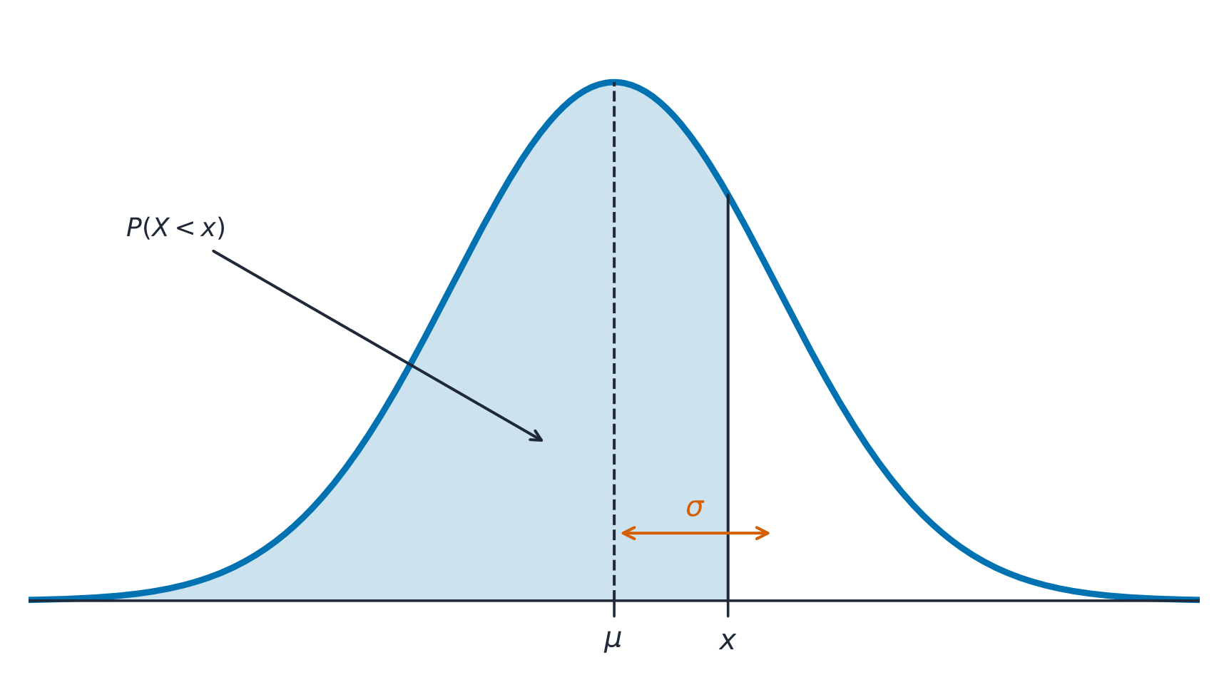
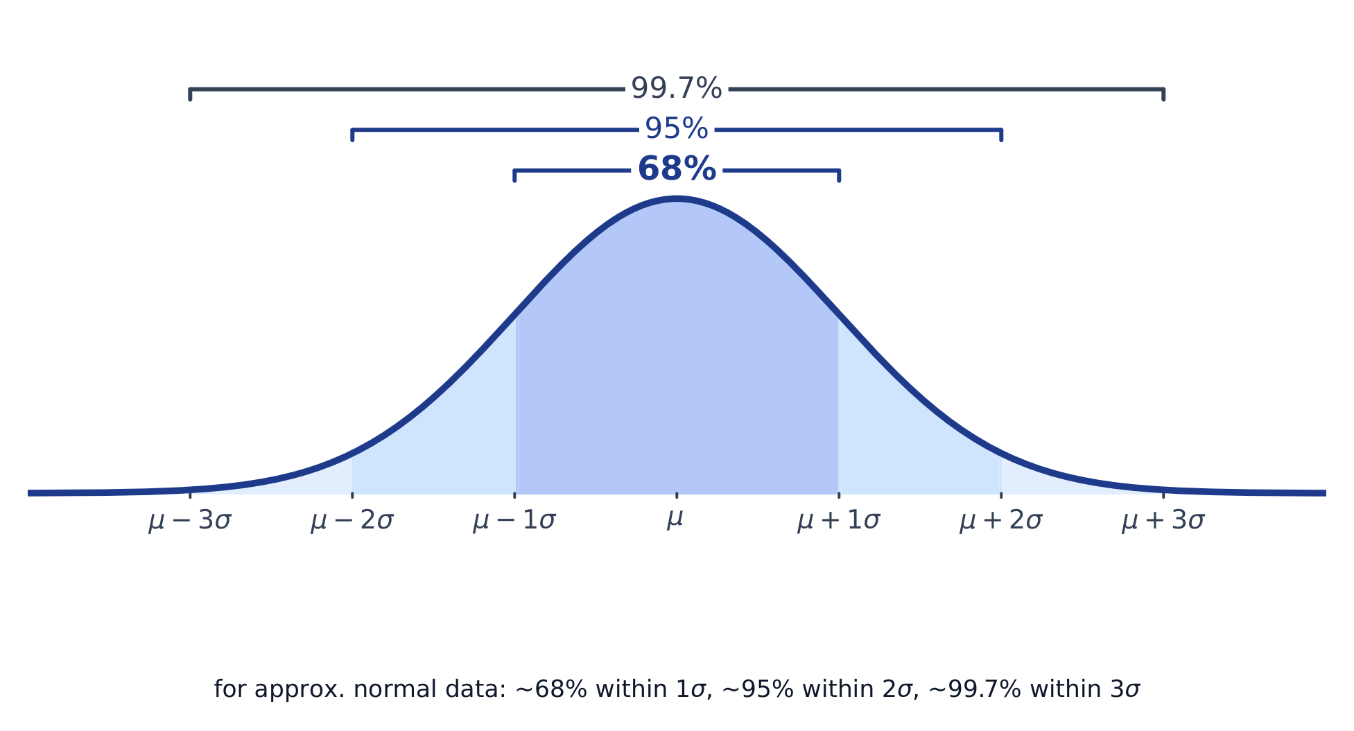
    A normal distribution 正态分布 is a symmetric, bell-shaped model described by its mean $\mu$ and standard deviation $\sigma$. The empirical rule 经验法则 (68–95–99.7): about 68% of values lie within $1\sigma$ of the mean, 95% within $2\sigma$, and 99.7% within $3\sigma$.

    The normal curve: a probability is the area under it, centred on the mean
    The normal curve: a probability is the area under it, centred on the mean

    A $z$-score 标准分数 measures how many standard deviations a value is from the mean:

    $$z=\frac{x-\mu}{\sigma}.$$
    Convert to a $z$-score, then use the normal table or technology to find the proportion (area) below, above, or between values – and reverse the process to find a value from a given percentile.

    Worked example. Test scores are normal with $\mu=500$ and $\sigma=100$. A score of $700$ has $z=\dfrac{700-500}{100}=2$. By the empirical rule, $95\%$ of scores lie within $2\sigma$, so $2.5\%$ lie above $700$ – meaning a $700$ is at about the $97.5$th percentile.

    The normal curve and the 68-95-99.7 empirical rule
    The normal curve and the 68-95-99.7 empirical rule
    Explore · ⁨Исследовать⁩

    Explore area under the normal curve · ⁨Исследуйте площадь под нормальным распределением⁩

    The proportion of data below a value equals the area under the curve to its left. Shade a tail or a central band to see the 68–95–99.7 empirical rule and read a $z$-score as an area. · ⁨"Пропорция" данных ниже значения равна "площади" под кривой слева от него. Выделите хвост или центральную полосу, чтобы увидеть эмпирическое правило «68–95–99,7» и считать $z$-балл как площадь.⁩

    Vocabulary · ⁨Словарь⁩ Train · ⁨Тренировать⁩
    English Русский
    normal distribution/ˈnɔːml ˌdɪstrɪˈbjuːʃn/ нормального распределения
    empirical rule/emˈpɪrɪkl ruːl/ эмпирическое правило
    $z$-score/ˈzed skɔː/ $z$-балл (Z-score)
    1.10

    Exam tips

    • Describe a distribution by shape, center, spread, and outliers (SOCS) — always in context.
    • The mean is pulled by outliers; the median resists them, so prefer the median for skewed data.
    • For a normal distribution use the 68–95–99.7 rule and z-scores $z=\tfrac{x-\mu}{\sigma}$.
    • Compare distributions with side-by-side boxplots and comment on center, spread, and shape.
    • Standard deviation measures a typical distance from the mean; the IQR pairs with the median.
  • 2

    Exploring Two-Variable Data · ⁨Исследование данных двух переменных⁩

    Watch lesson · ⁨Смотреть урок⁩
    2.1

    Are Two Variables Related? · ⁨Связаны ли две переменные?⁩

    Syllabus · ⁨Программа⁩
    English

    Enduring Understanding (VAR-1): Given that variation may be random or not, conclusions are uncertain.

    Learning Objective VAR-1.D: Identify questions to be answered about possible relationships in data. [Skill 1.A]

    • VAR-1.D.1 Apparent patterns and associations in data may be random or not.
    Русский

    Вечная идея (VAR-1): Поскольку вариация может быть случайной или нет, выводы остаются неопределенными.

    Учебная цель VAR-1.D: Определять вопросы для ответа о возможных связях в данных. [Навык 1.A]

    • VAR-1.D.1 Видимые закономерности и ассоциации в данных могут быть случайными или нет.

    Source: College Board AP Course and Exam Description · ⁨Источник: Описание курса и экзамена College Board AP⁩

    English

    Two-variable data let us ask whether two characteristics are associated 关联 – whether knowing one tells you something about the other. An explanatory variable 解释变量 (the "input") may help predict a response variable 响应变量 (the "output"). Association is not the same as causation.

    Русский

    Двухпеременные данные позволяют задать вопрос о том, связаны ли два признака ассоциированы ли они — говорит ли знание одной переменной о другой. Объясняющая переменная («входные данные») может помогать предсказать отзывчивую переменную («выходные данные»). Ассоциация не тождественна причинно-следственной связи.

    2.2

    Two Categorical Variables · ⁨Две категориальные переменные⁩

    Syllabus · ⁨Программа⁩
    English

    Enduring Understanding (UNC-1): Graphical representations and statistics allow us to identify and represent key features of data.

    Learning Objective UNC-1.P: Compare numerical and graphical representations for two categorical variables. [Skill 2.D]

    • UNC-1.P.1 Side-by-side bar graphs, segmented bar graphs, and mosaic plots are examples of bar graphs for one categorical variable, broken down by categories of another categorical variable.
    • UNC-1.P.2 Graphical representations of two categorical variables can be used to compare distributions and/or determine if variables are associated.
    • UNC-1.P.3 A two-way table, also called a contingency table, is used to summarize two categorical variables. The entries in the cells can be frequency counts or relative frequencies.
    • UNC-1.P.4 A joint relative frequency is a cell frequency divided by the total for the entire table.
    Русский

    Постоянное понимание (UNC-1): Графические представления и статистика позволяют нам выявлять и отображать ключевые особенности данных.

    Учебная цель UNC-1.P: Сравнивать числовые и графические представления для двух категориальных переменных. [Навык 2.D]

    • UNC-1.P.1 Боковые столбчатые диаграммы, сегментированные столбчатые диаграммы и мозаичные диаграммы являются примерами столбчатых диаграмм для одной категориальной переменной, разбитой по категориям другой категориальной переменной.
    • UNC-1.P.2 Графические представления двух категориальных переменных могут использоваться для сравнения распределений и/или определения того, связаны ли переменные.
    • UNC-1.P.3 Двусторонняя таблица, также называемая таблицей сопряженности, используется для обобщения двух категориальных переменных. Значения в ячейках могут быть подсчетами частот или относительными частотами.
    • UNC-1.P.4 Совместная относительная частота — это частота ячейки, деленная на общую сумму по всей таблице.

    Source: College Board AP Course and Exam Description · ⁨Источник: Описание курса и экзамена College Board AP⁩

    English

    A two-way table 双向表 (contingency table) counts individuals by two categorical variables at once. A marginal distribution 边缘分布 is a row or column total written as a fraction of the grand total (the totals themselves are just counts). Comparing the inside cells shows whether the variables are related.

    Русский

    Кросс-таблица (таблица сопряженности) подсчитывает количество индивидов по двум категориальным переменным одновременно. Маргинальное распределение — это итоговая сумма строки или столбца, выраженная в виде доли от общего итога (сами итоги — это просто подсчеты). Сравнение внутренних ячеек показывает, связаны ли переменные.

    2.3

    Comparing Groups with Conditional Distributions · ⁨Сравнение групп с условными распределениями⁩

    Syllabus · ⁨Программа⁩
    English

    Enduring Understanding (UNC-1): Graphical representations and statistics allow us to identify and represent key features of data.

    Learning Objective UNC-1.Q: Calculate statistics for two categorical variables. [Skill 2.C]

    • UNC-1.Q.1 The marginal relative frequencies are the row and column totals in a two-way table divided by the total for the entire table.
    • UNC-1.Q.2 A conditional relative frequency is a relative frequency for a specific part of the contingency table (e.g., cell frequencies in a row divided by the total for that row).

    Learning Objective UNC-1.R: Compare statistics for two categorical variables. [Skill 2.D]

    • UNC-1.R.1 Summary statistics for two categorical variables can be used to compare distributions and/or determine if variables are associated.
    Русский

    Постоянное понимание (UNC-1): Графические представления и статистика позволяют нам выявлять и отображать ключевые особенности данных.

    Цель обучения UNC-1.Q: Вычислять статистику для двух категориальных переменных. [Навык 2.C]

    • UNC-1.Q.1 Маргинальные относительные частоты — это суммы строк и столбцов в двусторонней таблице, деленные на общую сумму по всей таблице.
    • UNC-1.Q.2 Условная относительная частота — это относительная частота для конкретной части таблицы сопряженности (например, частоты ячеек в строке, деленные на итоговую сумму этой строки).

    Цель обучения UNC-1.R: Сравнивать статистику для двух категориальных переменных. [Навык 2.D]

    • UNC-1.R.1 Сводную статистику для двух категориальных переменных можно использовать для сравнения распределений и/или определения наличия связи между переменными.

    Source: College Board AP Course and Exam Description · ⁨Источник: Описание курса и экзамена College Board AP⁩

    English

    A conditional distribution 条件分布 is the distribution of one variable within a fixed category of the other (found by dividing each cell by its row or column total). If the conditional distributions differ across groups, the two variables are associated; if they are the same, there is no association. Segmented bar charts 分段条形图 or mosaic plots display them.

    Русский

    Условное распределение — это распределение одной переменной внутри фиксированной категории другой (находится путем деления каждой ячейки на итоговую сумму ее строки или столбца). Если условные распределения различаются между группами, две переменные ассоциированы; если они одинаковы, ассоциации нет. Сегментированные столбчатые диаграммы или мозаичные графики визуализируют их.

    2.4

    Scatterplots for Two Quantitative Variables · ⁨Диаграммы рассеяния для двух количественных переменных⁩

    Syllabus · ⁨Программа⁩
    English

    Enduring Understanding (UNC-1): Graphical representations and statistics allow us to identify and represent key features of data.

    Learning Objective UNC-1.S: Represent bivariate quantitative data using scatterplots. [Skill 2.B]

    • UNC-1.S.1 A bivariate quantitative data set consists of observations of two different quantitative variables made on individuals in a sample or population.
    • UNC-1.S.2 A scatterplot shows two numeric values for each observation, one corresponding to the value on the $x$-axis and one corresponding to the value on the $y$-axis.
    • UNC-1.S.3 An explanatory variable is a variable whose values are used to explain or predict corresponding values for the response variable.

    Enduring Understanding (DAT-1): Regression models may allow us to predict responses to changes in an explanatory variable.

    Learning Objective DAT-1.A: Describe the characteristics of a scatter plot. [Skill 2.A]

    • DAT-1.A.1 A description of a scatter plot includes form, direction, strength, and unusual features.
    • DAT-1.A.2 The direction of the association shown in a scatterplot, if any, can be described as positive or negative.
    • DAT-1.A.3 A positive association means that as values of one variable increase, the values of the other variable tend to increase. A negative association means that as values of one variable increase, values of the other variable tend to decrease.
    • DAT-1.A.4 The form of the association shown in a scatterplot, if any, can be described as linear or non-linear to varying degrees.
    • DAT-1.A.5 The strength of the association is how closely the individual points follow a specific pattern, e.g., linear, and can be shown in a scatterplot. Strength can be described as strong, moderate, or weak.
    • DAT-1.A.6 Unusual features of a scatter plot include clusters of points or points with relatively large discrepancies between the value of the response variable and a predicted value for the response variable.
    Русский

    Постоянное понимание (UNC-1): Графические представления и статистика позволяют нам выявлять и отображать ключевые особенности данных.

    Цель обучения UNC-1.S: Представлять бивариантные количественные данные с помощью точечных диаграмм. [Навык 2.B]

    • UNC-1.S.1 Набор бивариантных количественных данных состоит из наблюдений двух различных количественных переменных, полученных на индивидах из выборки или генеральной совокупности.
    • UNC-1.S.2 Точечная диаграмма показывает два числовых значения для каждого наблюдения: одно соответствует значению на оси $x$, а другое — значению на оси $y$.
    • UNC-1.S.3 Объясняющая переменная — это переменная, значения которой используются для объяснения или прогнозирования соответствующих значений откликающей переменной.

    Важное понимание (DAT-1): Модели регрессии могут позволить нам прогнозировать отклики на изменения объясняющей переменной.

    Цель обучения DAT-1.A: Описывать характеристики точечной диаграммы. [Навык 2.A]

    • DAT-1.A.1 Описание точечной диаграммы включает форму, направление, силу и необычные особенности.
    • DAT-1.A.2 Направление связи, показанной на точечной диаграмме (если оно есть), можно описать как положительное или отрицательное.
    • DAT-1.A.3 Положительная связь означает, что при увеличении значений одной переменной значения другой переменной имеют тенденцию к увеличению. Отрицательная связь означает, что при увеличении значений одной переменной значения другой переменной имеют тенденцию к уменьшению.
    • DAT-1.A.4 Форму связи, показанной на точечной диаграмме (если она есть), можно описать как линейную или нелинейную в той или иной степени.
    • DAT-1.A.5 Сила связи — это то, насколько близко отдельные точки следуют определенному шаблону, например, линейному, и может быть представлена на точечной диаграмме. Силу можно описать как сильную, умеренную или слабую.
    • DAT-1.A.6 Необычные особенности точечной диаграммы включают скопления точек или точки с относительно большими расхождениями между значением откликающей переменной и предсказанным значением для этой переменной.

    Source: College Board AP Course and Exam Description · ⁨Источник: Описание курса и экзамена College Board AP⁩

    English

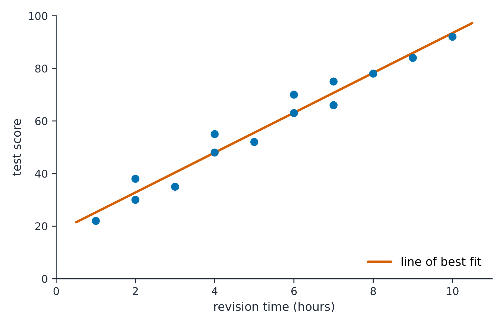
    A scatterplot 散点图 plots each individual as a point, explanatory variable on the $x$-axis and response on the $y$-axis. Describe it with DUFS: Direction (positive/negative), Unusual features (outliers, clusters), Form (linear or curved), and Strength (how tightly the points follow the pattern) – always in context.

    Русский

    На диаграмме рассеяния каждый отдельный элемент отображается точкой, объясняющая переменная откладывается по оси $x$, а отклика — по оси $y$. Опишите её с помощью DUFS: Направление (положительное/отрицательное), Необычные особенности (выбросы, скопления), Форма (линейная или криволинейная) и Сила (насколько плотно точки следуют за узором) — всегда в контексте.

    Линия тренда проходит через центр рассеянных точек
    Линия тренда проходит через центр рассеянных точек
    2.5

    Correlation · ⁨Корреляция⁩

    Syllabus · ⁨Программа⁩
    English

    Enduring Understanding (DAT-1): Regression models may allow us to predict responses to changes in an explanatory variable.

    Learning Objective DAT-1.B: Determine the correlation for a linear relationship. [Skill 2.C]

    • DAT-1.B.1 The correlation, $r$, gives the direction and quantifies the strength of the linear association between two quantitative variables.
    • DAT-1.B.2 The correlation coefficient can be calculated by: $r = \dfrac{1}{n-1} \sum \left( \dfrac{x_i - \bar{x}}{s_x} \right) \left( \dfrac{y_i - \bar{y}}{s_y} \right)$. However, the most common way to determine $r$ is by using technology.
    • DAT-1.B.3 A correlation coefficient close to 1 or $-1$ does not necessarily mean that a linear model is appropriate.

    Learning Objective DAT-1.C: Interpret the correlation for a linear relationship. [Skill 4.B]

    • DAT-1.C.1 The correlation, $r$, is unit-free, and always between $-1$ and 1, inclusive. A value of $r = 0$ indicates that there is no linear association. A value of $r = 1$ or $r = -1$ indicates that there is a perfect linear association.
    • DAT-1.C.2 A perceived or real relationship between two variables does not mean that changes in one variable cause changes in the other. That is, correlation does not necessarily imply causation.
    Русский

    Важное понимание (DAT-1): Модели регрессии могут позволить нам прогнозировать отклики на изменения объясняющей переменной.

    Цель обучения DAT-1.B: Определять корреляцию для линейной зависимости. [Навык 2.C]

    • DAT-1.B.1 Коэффициент корреляции, $r$, указывает направление и количественно оценивает силу линейной связи между двумя количественными переменными.
    • DAT-1.B.2 Коэффициент корреляции можно вычислить по формуле: $r = \dfrac{1}{n-1} \sum \left( \dfrac{x_i - \bar{x}}{s_x} \right) \left( \dfrac{y_i - \bar{y}}{s_y} \right)$. Однако наиболее распространенный способ определения $r$ — использование программного обеспечения.
    • DAT-1.B.3 Коэффициент корреляции, близкий к 1 или $-1$, не обязательно означает, что линейная модель является подходящей.

    Цель обучения DAT-1.C: Интерпретировать корреляцию для линейной зависимости. [Навык 4.B]

    • DAT-1.C.1 Коэффициент корреляции, $r$, безразмерен и всегда находится между $-1$ и 1 включительно. Значение $r = 0$ указывает на отсутствие линейной связи. Значение $r = 1$ или $r = -1$ указывает на идеальную линейную связь.
    • DAT-1.C.2 Воспринимаемая или реальная связь между двумя переменными не означает, что изменения одной переменной вызывают изменения другой. То есть корреляция не обязательно подразумевает причинно-следственную связь.

    Source: College Board AP Course and Exam Description · ⁨Источник: Описание курса и экзамена College Board AP⁩

    English
    What r actually measures

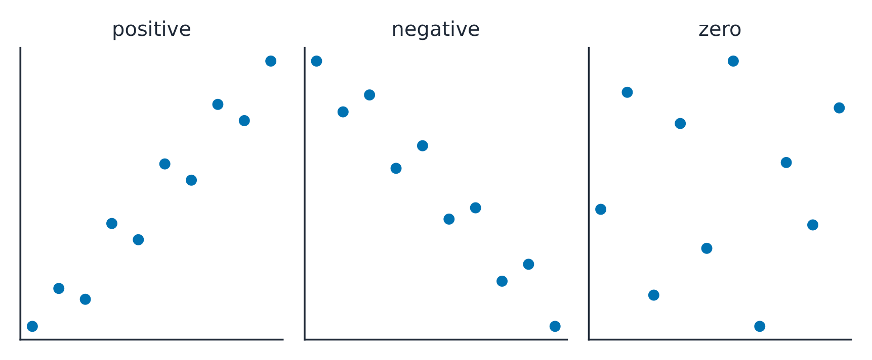
    The correlation coefficient 相关系数 $r$ measures the strength and direction of a linear relationship. It runs from $-1$ to $1$: near $\pm 1$ is strong linear, near $0$ is weak linear. $r$ has no units and does not change if you swap the variables. Warnings: $r$ only measures linear strength, it is not resistant to outliers, and a strong $r$ does not prove causation.

    Русский
    Что на самом деле измеряет r

    Коэффициент корреляции $r$ измеряет силу и направление линейной зависимости. Он изменяется от $-1$ до $1$: значение, близкое к $\pm 1$, указывает на сильную линейную связь, близкое к $0$ — на слабую. $r$ не имеет единиц измерения и не меняется при замене переменных местами. Предупреждения: $r$ измеряет линейную силу связи, она не устойчива к выбросам, и сильная $r$ не доказывает причинно-следственную связь.

    Положительная корреляция растет вместе; отрицательная движется в противоположных направлениях
    Положительная корреляция растет вместе; отрицательная движется в противоположных направлениях
    Explore · ⁨Исследовать⁩

    Strength of a linear relationship · ⁨Сила линейной связи⁩

    Correlation $r$ runs from $-1$ to $1$: near $\pm1$ the points hug a line, near 0 they scatter. Change it and watch the cloud tighten or spread. · ⁨Корреляция $r$ варьируется от $-1$ до $1$: близко к $\pm1$ точки лежат на прямой линии, близко к 0 они рассеяны. Измените коэффициент и наблюдайте, как облако точек сжимается или расширяется.⁩

    2.6

    Linear Regression Models · ⁨Линейные регрессионные модели⁩

    Syllabus · ⁨Программа⁩
    English

    Enduring Understanding (DAT-1): Regression models may allow us to predict responses to changes in an explanatory variable.

    Learning Objective DAT-1.D: Calculate a predicted response value using a linear regression model. [Skill 2.C]

    • DAT-1.D.1 A simple linear regression model is an equation that uses an explanatory variable, $x$, to predict the response variable, $y$.
    • DAT-1.D.2 The predicted response value, denoted by $\hat{y}$, is calculated as $\hat{y} = a + bx$, where $a$ is the $y$-intercept and $b$ is the slope of the regression line, and $x$ is the value of the explanatory variable.
    • DAT-1.D.3 Extrapolation is predicting a response value using a value for the explanatory variable that is beyond the interval of $x$-values used to determine the regression line. The predicted value is less reliable as an estimate the further we extrapolate.
    Русский

    Важное понимание (DAT-1): Модели регрессии могут позволить нам прогнозировать отклики на изменения объясняющей переменной.

    Цель обучения DAT-1.D: Вычислять предсказанное значение отклика с использованием модели линейной регрессии. [Навык 2.C]

    • DAT-1.D.1 Простая линейная модель регрессии — это уравнение, которое использует объясняющую переменную, $x$, для прогнозирования откликающей переменной, $y$.
    • DAT-1.D.2 Предсказанное значение отклика, обозначаемое как $\hat{y}$, рассчитывается по формуле $\hat{y} = a + bx$, где $a$ — точка пересечения с осью $y$, $b$ — угловой коэффициент линии регрессии, а $x$ — значение объясняющей переменной.
    • DAT-1.D.3 Экстраполяция — это предсказание значения отклика с использованием значения объясняющей переменной, выходящего за пределы интервала значений $x$, использованных для построения линии регрессии. Предсказанное значение становится менее надежным как оценка по мере того, как мы экстраполируем дальше.

    Source: College Board AP Course and Exam Description · ⁨Источник: Описание курса и экзамена College Board AP⁩

    English

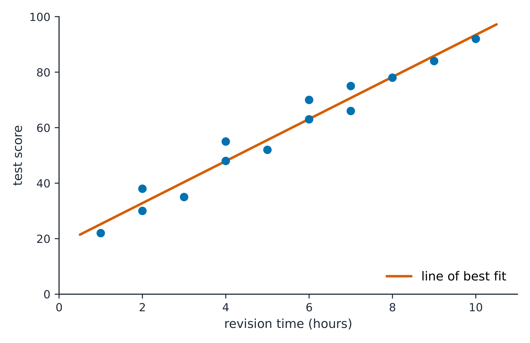
    The least-squares regression line 最小二乘回归线 predicts the response: $\hat{y}=a+bx$, where $\hat{y}$ is the predicted response. The slope 斜率 $b$ is the predicted change in $y$ per one-unit increase in $x$; the $y$-intercept 截距 $a$ is the predicted $y$ when $x=0$. Interpret both in context and with units – a graded skill. Avoid extrapolation 外推 (predicting far outside the data).

    Worked example. A study of hours studied ($x$) and test score ($y$) gives $\hat{y}=20+3x$. The slope means each extra hour of study is associated with a predicted $3$-point increase. A student who studies $5$ hours is predicted to score $\hat{y}=20+3(5)=35$.

    Русский

    Метод наименьших квадратов предсказывает отклик: $\hat{y}=a+bx$, где $\hat{y}$ — предсказанный отклик. Угол наклона $b$ означает предсказанное изменение $y$ при увеличении $x$ на одну единицу; $y$-пересечение (точка пересечения с осью y) $a$ — это предсказанный $y$ при $x=0$. Интерпретируйте оба параметра в контексте и с указанием единиц — это навык, требующий оценки. Избегайте экстраполяции (предсказания далеко за пределами имеющихся данных).

    Разобранный пример. Исследование часов учебы ($x$) и балла за тест ($y$) дало результат $\hat{y}=20+3x$. Угол наклона означает, что каждый дополнительный час учебы связан с предсказанным увеличением на $3$ баллов. Студент, который учился $5$ часа, по прогнозу получит $\hat{y}=20+3(5)=35$ баллов.

    Explore · ⁨Исследовать⁩

    Fit a least-squares line · ⁨Постройте линию наименьших квадратов⁩

    A regression line is the best straight-line fit, minimising the squared vertical distances. Its slope predicts how $y$ changes per unit of $x$. · ⁨Регрессионная прямая — это лучшая прямая линия, минимизирующая квадрат вертикальных расстояний. Её наклон предсказывает, как $y$ изменяется за единицу $x$.⁩

    2.7

    Residuals · ⁨Остатки⁩

    Syllabus · ⁨Программа⁩
    English

    Enduring Understanding (DAT-1): Regression models may allow us to predict responses to changes in an explanatory variable.

    Learning Objective DAT-1.E: Represent differences between measured and predicted responses using residual plots. [Skill 2.B]

    • DAT-1.E.1 The residual is the difference between the actual value and the predicted value: $\text{residual} = y - \hat{y}$.
    • DAT-1.E.2 A residual plot is a plot of residuals versus explanatory variable values or predicted response values.

    Learning Objective DAT-1.F: Describe the form of association of bivariate data using residual plots. [Skill 2.A]

    • DAT-1.F.1 Apparent randomness in a residual plot for a linear model is evidence of a linear form to the association between the variables.
    • DAT-1.F.2 Residual plots can be used to investigate the appropriateness of a selected model.
    Русский

    Важное понимание (DAT-1): Модели регрессии могут позволить нам прогнозировать отклики на изменения объясняющей переменной.

    Цель обучения DAT-1.E: Представлять разницы между измеренными и предсказанными откликами с помощью графиков остатков. [Навык 2.B]

    • DAT-1.E.1 Остаток — это разница между фактическим значением и предсказанным значением: $\text{residual} = y - \hat{y}$.
    • DAT-1.E.2 График остатков — это график остатков по значениям объясняющей переменной или предсказанным значениям отклика.

    Цель обучения DAT-1.F: Описывать форму связи бивариантных данных с помощью графиков остатков. [Навык 2.A]

    • DAT-1.F.1 Визуальная случайность на графике остатков для линейной модели является доказательством линейной формы связи между переменными.
    • DAT-1.F.2 Графики остатков могут использоваться для проверки уместности выбранной модели.

    Source: College Board AP Course and Exam Description · ⁨Источник: Описание курса и экзамена College Board AP⁩

    English
    Least-squares regression

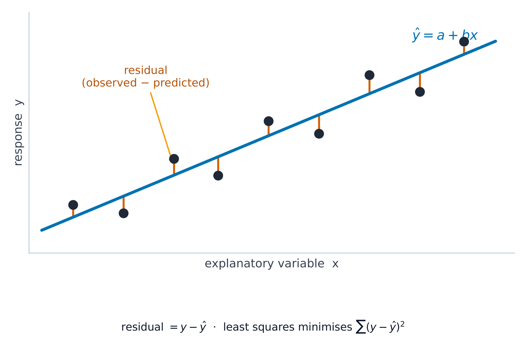
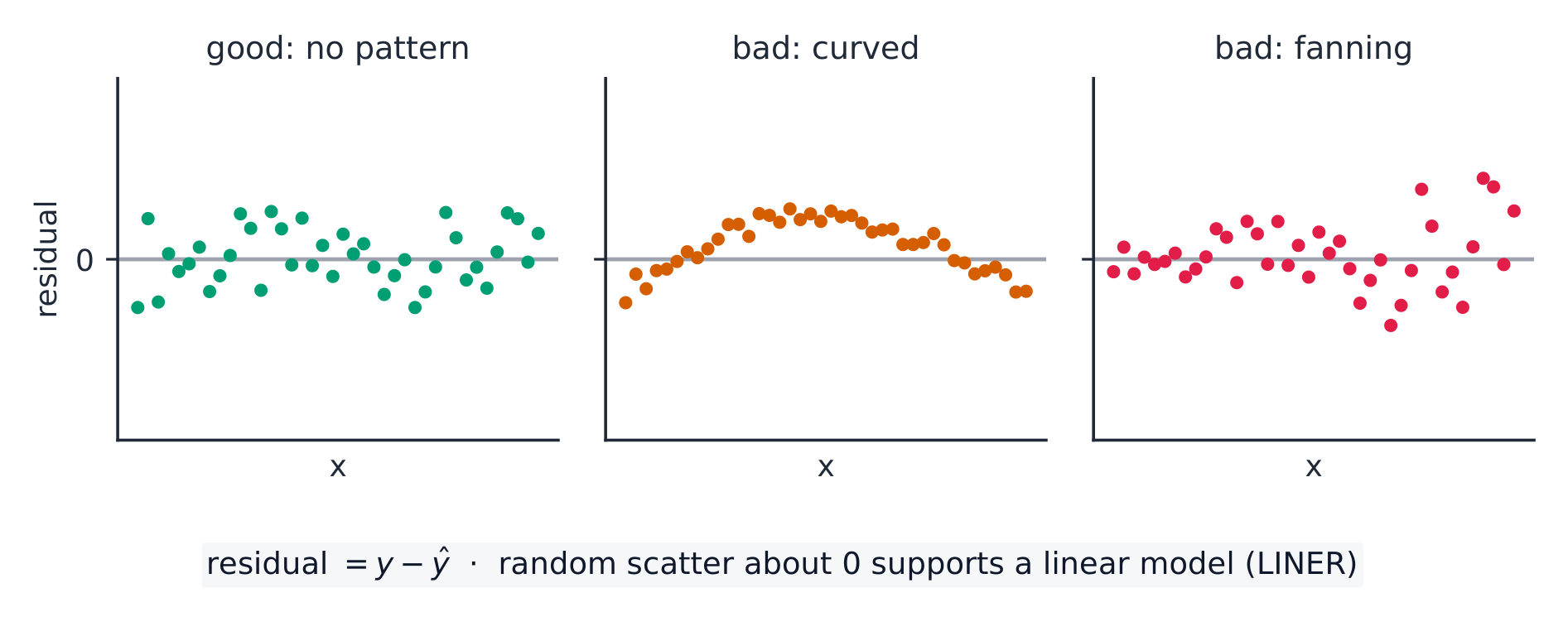
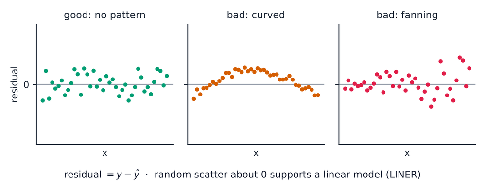
    A residual 残差 is actual minus predicted, $y-\hat{y}$: how far a point sits above (+) or below (−) the line. A residual plot 残差图 graphs residuals against $x$. If it shows no pattern (random scatter), a linear model is appropriate; a curved or fanning pattern means the linear model is a poor fit.

    Worked example. Continuing the study above, a student who studied $5$ hours actually scored $40$. The residual is $y-\hat{y}=40-35=+5$: the line under-predicted by $5$ points, so this point sits above the line.

    Русский
    Метод наименьших квадратов

    Остаток — это фактическое значение минус предсказанное, $y-\hat{y}$: расстояние, на которое точка находится выше (+) или ниже (−) линии. График остатков строит остатки по отношению к $x$. Если на графике нет закономерности (случайное рассеяние), линейная модель подходит; изогнутая или расширяющаяся форма указывает на плохое соответствие линейной модели.

    Разобранный пример. Продолжая исследование выше, студент, изучавший $5$ часов, фактически получил $40$ балл. Остаток составляет $y-\hat{y}=40-35=+5$: линия недооценила результат на $5$ баллов, поэтому эта точка находится выше линии.

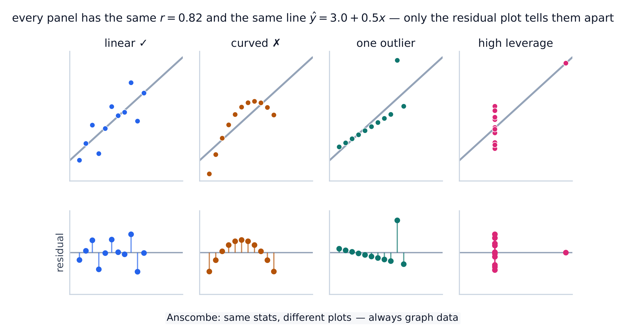
    Четыре набора данных с одинаковым r и линией регрессии, но четырьмя разными формами
    Предостережение относительно $r$ и линии: все четыре набора данных имеют одинаковый $r=0.82$ и одинаковую $\hat{y}=3.0+0.5x$, однако только первый является действительно линейным. Диаграммы рассеяния почти не отличаются — именно график остатков под каждой из них выявляет кривизну, выброс и точку с высоким влиянием.
    2.8

    Least-Squares Regression and Its Fit · ⁨Метод наименьших квадратов и его качество подгонки⁩

    Syllabus · ⁨Программа⁩
    English

    Enduring Understanding (DAT-1): Regression models may allow us to predict responses to changes in an explanatory variable.

    Learning Objective DAT-1.G: Estimate parameters for the least-squares regression line model. [Skill 2.C]

    • DAT-1.G.1 The least-squares regression model minimizes the sum of the squares of the residuals and contains the point $(\bar{x}, \bar{y})$.
    • DAT-1.G.2 The slope, $b$, of the regression line can be calculated as $b = r \left( \dfrac{s_y}{s_x} \right)$ where $r$ is the correlation between $x$ and $y$, $s_y$ is the sample standard deviation of the response variable, $y$, and $s_x$ is the sample standard deviation of the explanatory variable, $x$.
    • DAT-1.G.3 Sometimes, the $y$-intercept of the line does not have a logical interpretation in context.
    • DAT-1.G.4 In simple linear regression, $r^2$ is the square of the correlation, $r$. It is also called the coefficient of determination. $r^2$ is the proportion of variation in the response variable that is explained by the explanatory variable in the model.

    Learning Objective DAT-1.H: Interpret coefficients for the least-squares regression line model. [Skill 4.B]

    • DAT-1.H.1 The coefficients of the least-squares regression model are the estimated slope and $y$-intercept.
    • DAT-1.H.2 The slope is the amount that the predicted $y$-value changes for every unit increase in $x$.
    • DAT-1.H.3 The $y$-intercept value is the predicted value of the response variable when the explanatory variable is equal to $0$. The formula for the $y$-intercept, $a$, is $a = \bar{y} - b\bar{x}$.
    Русский

    Важное понимание (DAT-1): Модели регрессии могут позволить нам прогнозировать отклики на изменения объясняющей переменной.

    Цель обучения DAT-1.G: Оценивать параметры модели линии наименьших квадратов. [Навык 2.C]

    • DAT-1.G.1 Модель регрессии наименьших квадратов минимизирует сумму квадратов остатков и содержит точку $(\bar{x}, \bar{y})$.
    • DAT-1.G.2 Угловой коэффициент $b$ линии регрессии можно рассчитать как $b = r \left( \dfrac{s_y}{s_x} \right)$, где $r$ — корреляция между $x$ и $y$, $s_y$ — выборочное стандартное отклонение ответственной переменной, $y$, а $s_x$ — выборочное стандартное отклонение объясняющей переменной, $x$.
    • DAT-1.G.3 Иногда пересечение с осью $y$ (свободный член) не имеет логического толкования в контексте задачи.
    • DAT-1.G.4 В простой линейной регрессии $r^2$ является квадратом коэффициента корреляции, $r$. Он также называется коэффициентом детерминации. $r^2$ представляет собой долю вариации переменной отклика, которая объясняется объясняющей переменной в модели.

    Цель обучения DAT-1.H: Интерпретировать коэффициенты модели линии наименьших квадратов. [Навык 4.B]

    • DAT-1.H.1 Коэффициенты модели регрессии наименьших квадратов — это оцененный угловой коэффициент и пересечение с осью $y$.
    • DAT-1.H.2 Угловой коэффициент показывает величину изменения предсказанного значения по оси $y$ при увеличении переменной $x$ на одну единицу.
    • DAT-1.H.3 Значение пересечения с осью $y$ равно предсказанному значению переменной отклика, когда объясняющая переменная равна $0$. Формула для пересечения с осью $y$, $a$, имеет вид $a = \bar{y} - b\bar{x}$.

    Source: College Board AP Course and Exam Description · ⁨Источник: Описание курса и экзамена College Board AP⁩

    English

    The line minimizes the sum of squared residuals. Its fit is measured by:

    • $s$, the standard deviation of the residuals – the typical prediction error, in the response's units.
    • $r^2$, the coefficient of determination 决定系数 – the proportion of the variation in $y$ that the linear model explains (a value between $0$ and $1$; multiply by $100$ to state it as a percent). Report it in context: "$r^2 = 0.81$ means 81% of the variation in $y$ is explained by the linear relationship with $x$."
    Русский
    Линия наименьших квадратов минимизирует сумму квадратов остатков
    Линия наименьших квадратов минимизирует сумму квадратов остатков

    Линия минимизирует сумму квадратов остатков. Качество её подгонки оценивается следующим образом:

    • $s$, стандартное отклонение остатков — типичная ошибка предсказания, выраженная в единицах отклика.
    • $r^2$, коэффициент детерминации — доля вариации в $y$, объясненная линейной моделью (значение от $0$ до $1$; умножьте на $100$, чтобы выразить в процентах). Отчитывайте его в контексте: "$r^2 = 0.81$ означает, что 81% вариации в $y$ объясняется линейной зависимостью от $x$.""
    Vocabulary · ⁨Словарь⁩ Train · ⁨Тренировать⁩
    English Русский
    associated/əˈsəʊsɪeɪtɪd/ связаны
    explanatory variable/ekˈsplænətəri ˈveərɪəbl/ объясняющей переменной
    response variable/rɪˈspɒns ˈveərɪəbl/ переменной отклика
    two-way table/tuː weɪ ˈteɪbl/ двумерная таблица
    marginal distributions/ˈmɑːdʒɪnl ˌdɪstrɪˈbjuːʃnz/ маргинальные распределения
    conditional distribution/kənˈdɪʃənl ˌdɪstrɪˈbjuːʃn/ условное распределение
    Segmented bar charts/seɡˈmentɪd bɑː tʃɑːts/ Сегментированные столбчатые диаграммы
    scatterplot/ˈskætəplɒt/ диаграмма рассеяния
    correlation coefficient/ˌkɒrɪˈleɪʃn ˌkəʊɪˈfɪʃənt/ коэффициент корреляции
    least-squares regression line/liːst skweəz rɪˈɡreʃn laɪn/ метод наименьших квадратов (линия регрессии)
    slope/sləʊp/ наклоне графика
    y-intercept/waɪ ˌɪntəˈsept/ пересечение с осью y
    extrapolation/ekˈstræpəleɪʃn/ экстраполяция
    residual/rɪˈsɪdʒuːəl/ остатком
    residual plot/rɪˈsɪdʒuːəl plɒt/ график остатков
    coefficient of determination/ˌkəʊɪˈfɪʃənt ɒv dɪˌtɜːmɪˈneɪʃn/ коэффициент детерминации
    high-leverage/haɪ ˈliːvərɪdʒ/ высокая чувствительность (high-leverage)
    influential/ˌɪnfluːˈenʃl/ влияющий
    2.9

    Departures from Linearity · ⁨Отклонения от линейности⁩

    Syllabus · ⁨Программа⁩
    English

    Enduring Understanding (DAT-1): Regression models may allow us to predict responses to changes in an explanatory variable.

    Learning Objective DAT-1.I: Identify influential points in regression. [Skill 2.A]

    • DAT-1.I.1 An outlier in regression is a point that does not follow the general trend shown in the rest of the data and has a large residual when the Least Squares Regression Line (LSRL) is calculated.
    • DAT-1.I.2 A high-leverage point in regression has a substantially larger or smaller $x$-value than the other observations have.
    • DAT-1.I.3 An influential point in regression is any point that, if removed, changes the relationship substantially. Examples include much different slope, $y$-intercept, and/or correlation. Outliers and high leverage points are often influential.

    Learning Objective DAT-1.J: Calculate a predicted response using a least-squares regression line for a transformed data set. [Skill 2.C]

    • DAT-1.J.1 Transformations of variables, such as evaluating the natural logarithm of each value of the response variable or squaring each value of the explanatory variable, can be used to create transformed data sets, which may be more linear in form than the untransformed data.
    • DAT-1.J.2 Increased randomness in residual plots after transformation of data and/or movement of $r^2$ to a value closer to 1 offers evidence that the least-squares regression line for the transformed data is a more appropriate model to use to predict responses to the explanatory variable than the regression line for the untransformed data.
    Русский

    Важное понимание (DAT-1): Модели регрессии могут позволить нам прогнозировать отклики на изменения объясняющей переменной.

    Цель обучения DAT-1.I: Определять влияющие точки в регрессии. [Навык 2.A]

    • DAT-1.I.1 Выбросом в регрессии является точка, которая не следует общему тренду, наблюдаемому в остальных данных, и имеет большой остаток при расчете линии регрессии наименьших квадратов (LSRL).
    • DAT-1.I.2 Точка с высоким уровнем влияния (high-leverage point) в регрессии имеет значение по оси $x$, которое существенно больше или меньше значений у других наблюдений.
    • DAT-1.I.3 Влияющей точкой в регрессии является любая точка, удаление которой существенно изменяет зависимость. Примерами могут служить значительно отличающиеся угловые коэффициенты, пересечения с осью $y$ и/или коэффициенты корреляции. Выбросы и точки с высоким уровнем влияния часто являются влияющими.

    Цель обучения DAT-1.J: Рассчитывать предсказанный ответ с использованием линии наименьших квадратов для преобразованного набора данных. [Навык 2.C]

    • DAT-1.J.1 Преобразования переменных, такие как вычисление натурального логарифма каждого значения переменной отклика или возведение в квадрат каждого значения объясняющей переменной, могут использоваться для создания преобразованных наборов данных, которые могут быть более линейными по форме, чем исходные данные.
    • DAT-1.J.2 Увеличение случайности на графиках остатков после преобразования данных и/или приближение значения $r^2$ к значению, близкому к 1, свидетельствует о том, что линия регрессии наименьших квадратов для преобразованных данных является более подходящей моделью для предсказания ответов на объясняющую переменную, чем линия регрессии для исходных данных.

    Source: College Board AP Course and Exam Description · ⁨Источник: Описание курса и экзамена College Board AP⁩

    English

    Some points strongly affect the line. A high-leverage 高杠杆 point has an extreme $x$-value; an influential 有影响的 point noticeably changes the slope or $r$ when removed; an outlier here is a point with a large residual. When the pattern is curved, transform a variable (e.g. take a log) to straighten it, then fit a line to the transformed data.

    Русский

    Некоторые точки сильно влияют на линию. Точка с высоким влиянием имеет экстремальное значение по оси $x$; влияющая точка заметно меняет угол наклона или $r$ при удалении; выбросом здесь называется точка с большим остатком. Когда паттерн изогнут, преобразуйте переменную (например, возьмите логарифм), чтобы сделать зависимость линейной, затем подберите прямую к преобразованным данным.

    2.9

    Exam tips · ⁨Советы для экзамена⁩

    English
    • On a scatterplot describe direction, form, strength, and outliers; $r$ ranges $-1$ to $1$.
    • Correlation is not causation — a lurking variable can drive both.
    • Interpret the slope of the least-squares line in context ("per one unit of $x$, predicted $y$ changes by $b$").
    • Check a residual plot: no pattern means a line fits; a curve means it does not. Avoid extrapolation.
    • $r^2$ is the fraction of variation in $y$ explained by the model.
    Русский
    • На диаграмме рассеяния описывайте направление, форму, силу и выбросы; $r$ варьируется от $-1$ до $1$.
    • Корреляция не есть причинность — скрытая переменная может быть причиной обеих величин.
    • Интерпретируйте угол наклона линии наименьших квадратов в контексте ("при увеличении $x$ на одну единицу предсказанное значение $y$ изменяется на $b$").
    • Проверьте график остатков: отсутствие закономерности говорит о том, что прямая подходит; наличие кривой — что нет. Избегайте экстраполяции.
    • $r^2$ — доля вариации в $y$, объясненная моделью.
  • 3

    Collecting Data · ⁨Сбор данных⁩

    Watch lesson · ⁨Смотреть урок⁩
    3.1

    Can We Trust the Data We Collected? · ⁨Можно ли доверять собранным данным?⁩

    Syllabus · ⁨Программа⁩
    English

    Enduring Understanding (VAR-1): Given that variation may be random or not, conclusions are uncertain.

    Learning Objective VAR-1.E: Identify questions to be answered about data collection methods. [Skill 1.A]

    • VAR-1.E.1 Methods for data collection that do not rely on chance result in untrustworthy conclusions.
    Русский

    Вечная идея (VAR-1): Поскольку вариация может быть случайной или нет, выводы остаются неопределенными.

    Цель обучения VAR-1.E: Определять вопросы, которые необходимо ответить относительно методов сбора данных. [Навык 1.A]

    • VAR-1.E.1 Методы сбора данных, не основанные на случайном выборе, приводят к ненадежным выводам.

    Source: College Board AP Course and Exam Description · ⁨Источник: Описание курса и экзамена College Board AP⁩

    English

    A conclusion is only as good as the data behind it. How data are collected decides what you may conclude – whether you can generalize to a population 总体, and whether you can claim cause and effect. Poorly collected data can be worse than none.

    Русский

    Заключение так же хорошо, как и лежащие в его основе данные. Как собираются данные, определяет, какие выводы можно сделать — можно ли обобщать на генеральную совокупность и можно ли утверждать причинно-следственную связь. Плохо собранные данные могут быть хуже, чем их полное отсутствие.

    3.2

    Observational Studies and Experiments · ⁨Наблюдательные исследования и эксперименты⁩

    Syllabus · ⁨Программа⁩
    English

    Enduring Understanding (DAT-2): The way we collect data influences what we can and cannot say about a population.

    Learning Objective DAT-2.A: Identify the type of a study. [Skill 1.C]

    • DAT-2.A.1 A population consists of all items or subjects of interest.
    • DAT-2.A.2 A sample selected for study is a subset of the population.
    • DAT-2.A.3 In an observational study, treatments are not imposed. Investigators examine data for a sample of individuals (retrospective) or follow a sample of individuals into the future collecting data (prospective) in order to investigate a topic of interest about the population. A sample survey is a type of observational study that collects data from a sample in an attempt to learn about the population from which the sample was taken.
    • DAT-2.A.4 In an experiment, different conditions (treatments) are assigned to experimental units (participants or subjects).

    Learning Objective DAT-2.B: Identify appropriate generalizations and determinations based on observational studies. [Skill 4.A]

    • DAT-2.B.1 It is only appropriate to make generalizations about a population based on samples that are randomly selected or otherwise representative of that population.
    • DAT-2.B.2 A sample is only generalizable to the population from which the sample was selected.
    • DAT-2.B.3 It is not possible to determine causal relationships between variables using data collected in an observational study.
    Русский

    Устойчивое понимание (DAT-2): То, как мы собираем данные, влияет на то, что мы можем и не можем утверждать о популяции.

    Цель обучения DAT-2.A: Определять тип исследования. [Навык 1.C]

    • DAT-2.A.1 Популяция состоит из всех объектов или субъектов интереса.
    • DAT-2.A.2 Выборка, выбранная для исследования, является подмножеством популяции.
    • DAT-2.A.3 В наблюдательном исследовании воздействия (лечения) не вводятся. Исследователи анализируют данные для выборки индивидов (ретроспективно) или наблюдают за выборкой индивидов в будущем, собирая данные (проспективно), чтобы изучить интересующую тему о популяции. Выборочное обследование (sample survey) является видом наблюдательного исследования, который собирает данные у выборки, пытаясь узнать о популяции, из которой была выбрана эта выборка.
    • DAT-2.A.4 В эксперименте различные условия (воздействия) назначаются экспериментальным единицам (участникам или субъектам).

    Цель обучения DAT-2.B: Определять уместные обобщения и выводы на основе наблюдательных исследований. [Навык 4.A]

    • DAT-2.B.1 Обобщения о популяции уместны только на основе выборок, которые были случайно отобраны или иным образом репрезентативны для этой популяции.
    • DAT-2.B.2 Выборка репрезентативна (обобщима) только для той популяции, из которой она была выбрана.
    • DAT-2.B.3 Невозможно установить причинно-следственные связи между переменными, используя данные, собранные в наблюдательном исследовании.

    Source: College Board AP Course and Exam Description · ⁨Источник: Описание курса и экзамена College Board AP⁩

    English
    • In an observational study 观察性研究 you measure individuals without trying to influence them. It can show association, but not causation, because lurking variables may explain the link.
    • In an experiment 实验 you deliberately impose a treatment 处理 and compare responses. A well-designed experiment can establish cause and effect.
    Русский
    • В наблюдательном исследовании вы измеряете элементы, не пытаясь повлиять на них. Оно может показать ассоциацию, но не причинность, поскольку скрытые переменные могут объяснять эту связь.
    • В эксперименте вы преднамеренно вводите воздействие и сравниваете отклики. Хорошо спроектированный эксперимент может установить причинно-следственную связь.
    Explore · ⁨Исследовать⁩

    Observational study or experiment? · ⁨Наблюдательное исследование или эксперимент?⁩

    In an experiment the researcher imposes a treatment (and can show cause); an observational study only records what already happens (and can show association, not cause). · ⁨В эксперименте исследователь вводит лечение (и может показать причину); наблюдательное исследование лишь фиксирует то, что уже происходит (и может показать ассоциацию, но не причину).⁩

    3.3

    Random Sampling · ⁨Случайная выборка⁩

    Syllabus · ⁨Программа⁩
    English

    Enduring Understanding (DAT-2): The way we collect data influences what we can and cannot say about a population.

    Learning Objective DAT-2.C: Identify a sampling method, given a description of a study. [Skill 1.C]

    • DAT-2.C.1 When an item from a population can be selected only once, this is called sampling without replacement. When an item from the population can be selected more than once, this is called sampling with replacement.
    • DAT-2.C.2 A simple random sample (SRS) is a sample in which every group of a given size has an equal chance of being chosen. This method is the basis for many types of sampling mechanisms. A few examples of mechanisms used to obtain SRSs include numbering individuals and using a random number generator to select which ones to include in the sample, ignoring repeats, using a table of random numbers, or drawing a card from a deck without replacement.
    • DAT-2.C.3 A stratified random sample involves the division of a population into separate groups, called strata, based on shared attributes or characteristics (homogeneous grouping). Within each stratum a simple random sample is selected, and the selected units are combined to form the sample.
    • DAT-2.C.4 A cluster sample involves the division of a population into smaller groups, called clusters. Ideally, there is heterogeneity within each cluster, and clusters are similar to one another in their composition. A simple random sample of clusters is selected from the population to form the sample of clusters. Data are collected from all observations in the selected clusters.
    • DAT-2.C.5 A systematic random sample is a method in which sample members from a population are selected according to a random starting point and a fixed, periodic interval.
    • DAT-2.C.6 A census selects all items/subjects in a population.

    Learning Objective DAT-2.D: Explain why a particular sampling method is or is not appropriate for a given situation. [Skill 1.C]

    • DAT-2.D.1 There are advantages and disadvantages for each sampling method depending upon the question that is to be answered and the population from which the sample will be drawn.
    Русский

    Устойчивое понимание (DAT-2): То, как мы собираем данные, влияет на то, что мы можем и не можем утверждать о популяции.

    Цель обучения DAT-2.C: Определять метод выборки по описанию исследования. [Навык 1.C]

    • DAT-2.C.1 Когда объект из популяции может быть выбран только один раз, это называется выборкой без возвращения. Когда объект из популяции может быть выбран более одного раза, это называется выборкой с возвращением.
    • DAT-2.C.2 Простая случайная выборка (SRS) — это выборка, в которой каждая группа заданного размера имеет одинаковый шанс быть выбранной. Этот метод лежит в основе многих типов механизмов выборки. Несколько примеров механизмов, используемых для получения SRS, включают нумерацию индивидов и использование генератора случайных чисел для выбора тех, кого включить в выборку, игнорируя повторы, использование таблицы случайных чисел или вытягивание карточки из колоды без возвращения.
    • DAT-2.C.3 Стратифицированная случайная выборка предполагает разделение популяции на отдельные группы, называемые стратами, на основе общих атрибутов или характеристик (гомогенное группирование). Внутри каждой страты выбирается простая случайная выборка, а выбранные единицы объединяются для формирования итоговой выборки.
    • DAT-2.C.4 Кластерная выборка предполагает разделение популяции на меньшие группы, называемые кластерами. В идеале внутри каждого кластера должна присутствовать гетерогенность, а сами кластеры должны быть схожи друг с другом по своему составу. Из популяции выбирается простая случайная выборка кластеров, которая и формирует выборку кластеров. Данные собираются со всех наблюдений в выбранных кластерах.
    • DAT-2.C.5 Систематическая случайная выборка — это метод, при котором члены выборки из популяции отбираются согласно случайному начальному пункту и фиксированному периодическому интервалу.
    • DAT-2.C.6 Перепись охватывает все элементы/объекты в популяции.

    Учебная цель DAT-2.D: Объяснить, почему тот или иной метод выборки является подходящим или неподходящим для данной ситуации. [Навык 1.C]

    • DAT-2.D.1 Для каждого метода выборки существуют преимущества и недостатки, зависящие от вопроса, на который необходимо ответить, и популяции, из которой будет выбрана выборка.

    Source: College Board AP Course and Exam Description · ⁨Источник: Описание курса и экзамена College Board AP⁩

    English

    To learn about a population you take a sample 样本. Random sampling 随机抽样 protects against selection bias 偏差 and lets you generalize (it cannot fix undercoverage, nonresponse, or response bias — see below). Common designs:

    • Simple random sample (SRS) 简单随机样本: every group of the chosen size is equally likely.
    • Stratified 分层: split the population into similar strata, then sample within each.
    • Cluster 整群: split into clusters, randomly choose whole clusters.
    • Systematic 系统: pick every $k$th individual from a random start.

    A convenience sample 方便样本 or voluntary response sample is not random and is biased.

    Worked example. To survey a school, an administrator lists all students by grade and randomly selects $20$ from each grade. This is a stratified sample – the grades are the strata – which guarantees every grade is represented, unlike an SRS that might by chance draw few from one grade.

    Русский

    Для изучения генеральной совокупности вы берете выборку. Случайная выборка защищает от систематической ошибки отбора и позволяет делать обобщения (она не устраняет неполного покрытия, отсутствия ответа или смещения в ответах — см. ниже). Распространенные методы:

    • Простая случайная выборка (SRS): любая группа выбранного размера имеет равную вероятность быть выбранной.
    • Стратифицированная: разделите совокупность на однородные страты, затем сделайте выборку внутри каждой.
    • Кластерная: разделите на кластеры, случайно выберите целые кластеры.
    • Систематическая: выбирайте каждого $k$-го элемента после случайного начала.
    Четыре метода случайной выборки: кто попадает в выборку и как
    Четыре метода случайной выборки: кто отбирается и как

    Удобная выборка или выборка добровольцев не является случайной и содержит смещение.

    Разобранное решение. Для опроса школы администратор перечисляет всех учеников по классам и случайно выбирает $20$ из каждого класса. Это стратифицированная выборка — классы являются стратами, — что гарантирует представление каждого класса, в отличие от SRS (простой случайной выборки), которая может случайно включить мало учеников из одного класса.

    Случайные исходы: при бросании игральной кости все грани имеют равную вероятность в честных условиях
    Случайные исходы: при честных условиях игральная кость делает каждую грань равновероятной
    3.4

    When Sampling Goes Wrong · ⁨Когда выборка дала сбой⁩

    Syllabus · ⁨Программа⁩
    English

    Enduring Understanding (DAT-2): The way we collect data influences what we can and cannot say about a population.

    Learning Objective DAT-2.E: Identify potential sources of bias in sampling methods. [Skill 1.C]

    • DAT-2.E.1 Bias occurs when certain responses are systematically favored over others.
    • DAT-2.E.2 When a sample is comprised entirely of volunteers or people who choose to participate, the sample will typically not be representative of the population (voluntary response bias).
    • DAT-2.E.3 When part of the population has a reduced chance of being included in the sample, the sample will typically not be representative of the population (undercoverage bias).
    • DAT-2.E.4 Individuals chosen for the sample for whom data cannot be obtained (or who refuse to respond) may differ from those for whom data can be obtained (nonresponse bias).
    • DAT-2.E.5 Problems in the data gathering instrument or process result in response bias. Examples include questions that are confusing or leading (question wording bias) and self-reported responses.
    • DAT-2.E.6 Non-random sampling methods (for example, samples chosen by convenience or voluntary response) introduce potential for bias because they do not use chance to select the individuals.
    Русский

    Устойчивое понимание (DAT-2): То, как мы собираем данные, влияет на то, что мы можем и не можем утверждать о популяции.

    Учебная цель DAT-2.E: Определить потенциальные источники смещения в методах выборки. [Навык 1.C]

    • DAT-2.E.1 Смещение возникает, когда определенные ответы систематически предпочтительнее других.
    • DAT-2.E.2 Когда выборка состоит исключительно из добровольцев или людей, решивших принять участие, она, как правило, не представляет популяцию (смещение добровольного ответа).
    • DAT-2.E.3 Когда часть популяции имеет сниженную вероятность попадания в выборку, она, как правило, не представляет популяцию (смещение неполного покрытия).
    • DAT-2.E.4 Индивидуумы, выбранные для выборки, у которых невозможно получить данные (или которые отказываются отвечать), могут отличаться от тех, у кого данные получены (смещение невключения в ответе).
    • DAT-2.E.5 Проблемы в инструменте или процессе сбора данных приводят к смещению в ответах. Примерами являются вопросы, вызывающие путаницу или подталкивающие к определенному ответу (смещение формулировки вопросов) и самооценочные ответы.
    • DAT-2.E.6 Неслучайные методы выборки (например, выборки, выбранные по удобству или методом добровольного ответа) создают потенциал для смещения, поскольку они не используют случайность для выбора индивидов.

    Source: College Board AP Course and Exam Description · ⁨Источник: Описание курса и экзамена College Board AP⁩

    English

    Bias makes estimates systematically miss the truth:

    • Undercoverage 覆盖不足: some groups are left out of the sampling frame.
    • Nonresponse 无回应: selected people do not answer.
    • Response bias 回应偏差: people answer inaccurately (bad wording, sensitive topics).

    Bias is about a consistent error in one direction – increasing the sample size does not fix it.

    Русский

    Смещение приводит к систематическому отклонению оценок от истины:

    • Недостаточное покрытие: некоторые группы не включены в список выборки.
    • Отказ от ответа: выбранные люди не отвечают на вопросы.
    • Смещение ответов: люди дают неточные ответы (плохая формулировка вопросов, чувствительные темы).

    Смещение — это систематическая ошибка в одном направлении; увеличение размера выборки её не устраняет.

    Удобные выборки не представляют генеральную совокупность: смещение возникает, когда отбор не является случайным
    Удобные выборки не отражают генеральную совокупность: смещение появляется при нерандомном отборе
    Vocabulary · ⁨Словарь⁩ Train · ⁨Тренировать⁩
    English Русский
    bias/ˈbaɪəs/ предвзятость
    Simple random sample (SRS)/ˈsɪmpl ˈrændəm ˈsæmpl/ простая случайная выборка (SRS)
    Stratified/ˈstrætɪfaɪd/ Стратифицированная
    Cluster/ˈklʌstə/ Кластерная
    Systematic/ˌsɪstəˈmætɪk/ Систематическая
    convenience sample/kənˈviːnɪəns ˈsæmpl/ удобная выборка
    Undercoverage/ˌʌndəˈkʌvərɪdʒ/ неполное покрытие
    Nonresponse/ˌnɒnrɪˈspɒns/ отказ от участия в опросе
    Response bias/rɪˈspɒns ˈbaɪəs/ смещение при ответе
    control group/kənˈtrəʊl ɡruːp/ контрольная группа
    placebo/pləˈsiːbəʊ/ плацебо
    Random assignment/ˈrændəm əˈsaɪnmənt/ случайное распределение
    Replication/ˌreplɪˈkeɪʃn/ Репликация
    3.5

    Designing an Experiment · ⁨Проектирование эксперимента⁩

    Syllabus · ⁨Программа⁩
    English

    Enduring Understanding (VAR-3): Well-designed experiments can establish evidence of causal relationships.

    Learning Objective VAR-3.A: Identify the components of an experiment. [Skill 1.C]

    • VAR-3.A.1 The experimental units are the individuals (which may be people or other objects of study) that are assigned treatments. When experimental units consist of people, they are sometimes referred to as participants or subjects.
    • VAR-3.A.2 An explanatory variable (or factor) in an experiment is a variable whose levels are manipulated intentionally. The levels or combination of levels of the explanatory variable(s) are called treatments.
    • VAR-3.A.3 A response variable in an experiment is an outcome from the experimental units that is measured after the treatments have been administered.
    • VAR-3.A.4 A confounding variable in an experiment is a variable that is related to the explanatory variable and influences the response variable and may create a false perception of association between the two.

    Learning Objective VAR-3.B: Describe elements of a well-designed experiment. [Skill 1.B]

    • VAR-3.B.1 A well-designed experiment should include the following:
      • a. Comparisons of at least two treatment groups, one of which could be a control group.
      • b. Random assignment/allocation of treatments to experimental units.
      • c. Replication (more than one experimental unit in each treatment group).
      • d. Control of potential confounding variables where appropriate.

    Learning Objective VAR-3.C: Compare experimental designs and methods. [Skill 1.C]

    • VAR-3.C.1 In a completely randomized design, treatments are assigned to experimental units completely at random. Random assignment tends to balance the effects of uncontrolled (confounding) variables so that differences in responses can be attributed to the treatments.
    • VAR-3.C.2 Methods for randomly assigning treatments to experimental units in a completely randomized design include using a random number generator, a table of random values, drawing chips without replacement, etc.
    • VAR-3.C.3 In a single-blind experiment, subjects do not know which treatment they are receiving, but members of the research team do, or vice versa.
    • VAR-3.C.4 In a double-blind experiment neither the subjects nor the members of the research team who interact with them know which treatment a subject is receiving.
    • VAR-3.C.5 A control group is a collection of experimental units either not given a treatment of interest or given a treatment with an inactive substance (placebo) in order to determine if the treatment of interest has an effect.
    • VAR-3.C.6 The placebo effect occurs when experimental units have a response to a placebo.
    • VAR-3.C.7 For randomized complete block designs, treatments are assigned completely at random within each block.
    • VAR-3.C.8 Blocking ensures that at the beginning of the experiment the units within each block are similar to each other with respect to at least one blocking variable. A randomized block design helps to separate natural variability from differences due to the blocking variable.
    • VAR-3.C.9 A matched pairs design is a special case of a randomized block design. Using a blocking variable, subjects (whether they are people or not) are arranged in pairs matched on relevant factors. Matched pairs may be formed naturally or by the experimenter. Every pair receives both treatments by randomly assigning one treatment to one member of the pair and subsequently assigning the remaining treatment to the second member of the pair. Alternately, each subject may get both treatments.
    Русский

    Вечная истина (VAR-3): Хорошо спланированные эксперименты могут установить доказательства причинно-следственных связей.

    Учебная цель VAR-3.A: Определить компоненты эксперимента. [Навык 1.C]

    • VAR-3.A.1 Экспериментальные единицы — это индивидуумы (которые могут быть людьми или другими объектами исследования), которым назначаются воздействия. Когда экспериментальные единицы состоят из людей, их иногда называют участниками или субъектами.
    • VAR-3.A.2 Объясняющая переменная (или фактор) в эксперименте — это переменная, уровни которой намеренно манипулируются. Уровни или комбинация уровней объясняющей переменной(ых) называются воздействиями (обработками).
    • VAR-3.A.3 Откликующая переменная в эксперименте — это результат от экспериментальных единиц, который измеряется после того, как были применены воздействия.
    • VAR-3.A.4 Спутанная переменная в эксперименте — это переменная, связанная с объясняющей переменной и влияющая на откликующую переменную, что может создать ложное восприятие связи между двумя переменными.

    Учебная цель VAR-3.B: Описать элементы хорошо спланированного эксперимента. [Навык 1.B]

    • VAR-3.B.1 Хорошо спланированный эксперимент должен включать следующее:
      • a. Сравнение как минимум двух групп воздействий, одной из которых может быть контрольная группа.
      • b. Случайное назначение/распределение воздействий экспериментальным единицам.
      • c. Репликация (более чем одна экспериментальная единица в каждой группе воздействий).
      • d. Контроль потенциальных спутанных переменных там, где это уместно.

    Учебная цель VAR-3.C: Сравнивать экспериментальные дизайны и методы. [Навык 1.C]

    • VAR-3.C.1 В полностью рандомизированном дизайне воздействия назначаются экспериментальным единицам полностью случайно. Случайное назначение tends to balance the effects of uncontrolled (confounding) variables so that differences in responses can be attributed to the treatments.
    • VAR-3.C.2 Методы случайного назначения воздействий экспериментальным единицам в полностью рандомизированном дизайне включают использование генератора случайных чисел, таблицу случайных значений, вытягивание жетонов без возвращения и т. д.
    • VAR-3.C.3 В однослепом эксперименте субъекты не знают, какое воздействие они получают, но члены исследовательской команды знают, или наоборот.
    • VAR-3.C.4 В двуслепом эксперименте ни субъекты, ни члены исследовательской команды, взаимодействующие с ними, не знают, какое воздействие получает субъект.
    • VAR-3.C.5 Контрольная группа — это совокупность экспериментальных единиц, которым либо не назначают интересующее воздействие, либо назначают воздействие с неактивным веществом (плацебо) для определения того, оказывает ли интересующее воздействие эффект.
    • VAR-3.C.6 Эффект плацебо возникает, когда экспериментальные единицы демонстрируют реакцию на плацебо.
    • VAR-3.C.7 Для рандомизированных полных блочных дизайнов воздействия назначаются полностью случайно внутри каждого блока.
    • VAR-3.C.8 Блокирование обеспечивает то, что в начале эксперимента единицы внутри каждого блока похожи друг на друга по крайней мере относительно одной блокирующей переменной. Рандомизированный блочный дизайн помогает разделить естественную изменчивость на различия, обусловленные блокирующей переменной.
    • VAR-3.C.9 План с парными сравнениями является частным случаем плана со случайной блокировкой. С использованием блокирующей переменной субъекты (независимо от того, являются ли они людьми или нет) группируются в пары, сопоставленные по релевантным факторам. Пары могут формироваться естественным образом или экспериментатором. Каждая пара получает оба лечения путем случайного назначения одного лечения одному участнику пары и последующего назначения оставшегося лечения второму участнику пары. Альтернативно, каждый субъект может получить оба лечения.

    Source: College Board AP Course and Exam Description · ⁨Источник: Описание курса и экзамена College Board AP⁩

    English

    Good experiments follow three principles:

    • Comparison with a control group 对照组 (often a placebo 安慰剂).
    • Random assignment 随机分配 of subjects to treatments, to balance out other variables.
    • Replication 重复: enough subjects per treatment to see a real effect.

    Confounding 混杂 occurs when another variable is tied to the treatment so their effects cannot be separated; random assignment guards against it. Blinding 盲法 hides who is getting which treatment to prevent expectation effects: in a single-blind 单盲 study only one side is kept unaware (usually the subjects, or only the people assessing the result), while in a double-blind 双盲 study neither the subjects nor the researchers who interact with them know, blocking both the placebo effect and biased assessment. Blocking 区组 groups similar subjects and randomizes within each block to reduce variability.

    Русский

    Хорошие эксперименты следуют трём принципам:

    • Сравнение с контрольной группой (часто плацебо).
    • Случайное назначение испытуемых к treatments для выравнивания других переменных.
    • Репликация: достаточное количество испытуемых на каждое treatment, чтобы увидеть реальный эффект.
    Полностью рандомизированный эксперимент сравнивает группу, получавшую лечение, с контрольной группой
    Полностью рандомизированный эксперимент сравнивает группу лечения с контрольной группой

    Смешивающий фактор (confounding) возникает, когда другая переменная связана с treatment так, что их эффекты невозможно разделить; случайное назначение защищает от этого. Ослепление скрывает, кто получает какое treatment, чтобы предотвратить эффекты ожидания: в одиночном ослеплении одна сторона остаётся в неведении (обычно испытуемые или только те, кто оценивает результат), а в двойном ослеплении ни испытуемые, ни исследователи, взаимодействующие с ними, не знают, что блокирует как эффект плацебо, так и предвзятую оценку. Блокирование группирует похожих испытуемых и рандомизирует внутри каждого блока для снижения вариабельности.

    Клинический испытание: случайное назначение разделяет группы лечения и контроля
    Клинические испытания: случайное назначение отделяет treatment от контроля
    Vocabulary · ⁨Словарь⁩ Train · ⁨Тренировать⁩
    English Русский
    population/ˌpɒpjʊˈleɪʃn/ населением
    observational study/ɒbzəˈveɪʃənl ˈstʌdi/ наблюдательное исследование
    experiment/ekˈsperɪmənt/ эксперимент
    treatment/ˈtriːtmənt/ воздействие
    sample/ˈsæmpl/ выборка
    Random sampling/ˈrændəm ˈsæmplɪŋ/ Случайная выборка
    Confounding/kənˈfaʊndɪŋ/ смешивающий фактор
    Blinding/ˈblaɪndɪŋ/ ослепление
    single-blind/ˈsɪŋɡl blaɪnd/ одиночный слепой метод
    double-blind/ˈdʌbl blaɪnd/ двойной слепой метод
    Blocking/ˈblɒkɪŋ/ блокировка
    3.6

    Choosing the Right Design · ⁨Выбор правильного дизайна⁩

    Syllabus · ⁨Программа⁩
    English

    Enduring Understanding (VAR-3): Well-designed experiments can establish evidence of causal relationships.

    Learning Objective VAR-3.D: Explain why a particular experimental design is appropriate. [Skill 1.C]

    • VAR-3.D.1 There are advantages and disadvantages for each experimental design depending on the question of interest, the resources available, and the nature of the experimental units.
    Русский

    Вечная истина (VAR-3): Хорошо спланированные эксперименты могут установить доказательства причинно-следственных связей.

    Цель обучения VAR-3.D: Объяснить, почему тот или иной экспериментальный дизайн является подходящим. [Навык 1.C]

    • VAR-3.D.1 Для каждого экспериментального дизайна есть преимущества и недостатки, зависящие от интересующего вопроса, доступных ресурсов и природы экспериментальных единиц.

    Source: College Board AP Course and Exam Description · ⁨Источник: Описание курса и экзамена College Board AP⁩

    English

    Match the design to the goal: use a completely randomized design for uniform subjects; a randomized block design when a known variable (sex, age) affects the response; a matched-pairs design when each subject can serve as its own control. State how you would carry out the randomization.

    Русский

    Соотнесите дизайн с целью: используйте полностью рандомизированный дизайн для однородных испытуемых; рандомизированный блочный дизайн, когда известная переменная (пол, возраст) влияет на результат; дизайн парных сравнений, когда каждый испытуемый может служить собственной контрольной группой. Опишите, как вы будете проводить рандомизацию.

    3.7

    What an Experiment Lets You Conclude · ⁨Что позволяет заключить эксперимент⁩

    Syllabus · ⁨Программа⁩
    English

    Enduring Understanding (VAR-3): Well-designed experiments can establish evidence of causal relationships.

    Learning Objective VAR-3.E: Interpret the results of a well-designed experiment. [Skill 4.B]

    • VAR-3.E.1 Statistical inference attributes conclusions based on data to the distribution from which the data were collected.
    • VAR-3.E.2 Random assignment of treatments to experimental units allows researchers to conclude that some observed changes are so large as to be unlikely to have occurred by chance. Such changes are said to be statistically significant.
    • VAR-3.E.3 Statistically significant differences between or among experimental treatment groups are evidence that the treatments caused the effect.
    • VAR-3.E.4 If the experimental units used in an experiment are representative of some larger group of units, the results of an experiment can be generalized to the larger group. Random selection of experimental units gives a better chance that the units will be representative.
    Русский

    Вечная истина (VAR-3): Хорошо спланированные эксперименты могут установить доказательства причинно-следственных связей.

    Цель обучения VAR-3.E: Интерпретировать результаты хорошо спланированного эксперимента. [Навык 4.B]

    • VAR-3.E.1 Статистический вывод приписывает выводы, основанные на данных, распределению, из которого были собраны эти данные.
    • VAR-3.E.2 Случайное назначение treatments экспериментальным единицам позволяет исследователям сделать вывод о том, что некоторые наблюдаемые изменения настолько велики, что маловероятно, что они произошли случайно. Такие изменения называются статистически значимыми.
    • VAR-3.E.3 Статистически значимые различия между или среди групп экспериментальных treatments являются доказательством того, что treatments вызвали эффект.
    • VAR-3.E.4 Если экспериментальные единицы, использованные в эксперименте, репрезентативны для некоторой более крупной группы единиц, результаты эксперимента можно обобщить на эту более крупную группу. Случайный выбор экспериментальных единиц дает больше шансов, что они будут репрезентативными.

    Source: College Board AP Course and Exam Description · ⁨Источник: Описание курса и экзамена College Board AP⁩

    English

    Two questions decide the scope of a conclusion:

    • Random assignment used? Then a significant difference can be attributed to the treatment (causation) – for these subjects.
    • Random sampling from a population? Then results generalize to that population.

    Only an experiment with random assignment supports a cause-and-effect claim; only random sampling supports generalization. Say exactly which you have.

    Worked example. Researchers randomly assign $100$ volunteers to a new drug or a placebo, and the drug group improves significantly more. Because of the random assignment, the improvement can be attributed to the drug (causation) – but because the subjects were not randomly sampled, the conclusion applies only to these volunteers and does not automatically generalize to everyone.

    Русский

    Два вопроса определяют границы вывода:

    • Использовано ли случайное назначение? Тогда значимая разница может быть приписана treatment (причинно-следственная связь) — для этих испытуемых.
    • Проведён ли случайный отбор из генеральной совокупности? Тогда результаты распространяются на эту совокупность.

    Только эксперимент со случайным назначением поддерживает утверждение о причинно-следственной связи; только случайный отбор поддерживает обобщение. Укажите точно, что именно у вас есть.

    Разобранное решение. Исследователи случайно назначают $100$ добровольцев на получение нового препарата или плацебо, и группа, получавшая препарат, значительно лучше улучшается. Благодаря случайному назначению улучшение можно приписать препарату (причинно-следственная связь) — но поскольку испытуемые не были случайно выбраны, вывод применим только к этим добровольцам и автоматически не распространяется на всех остальных.

    3.7

    Exam tips · ⁨Советы для экзамена⁩

    English
    • Distinguish an observational study (finds association) from an experiment (can show causation).
    • Good sampling is random (SRS, stratified, cluster) — beware bias (voluntary response, undercoverage, nonresponse).
    • Good experiments use control, randomization, and replication; blocking handles a known nuisance variable.
    • Only a randomized experiment supports a cause-and-effect conclusion.
    • Name the population, sample, and any confounding clearly.
    Русский
    • Различайте наблюдательное исследование (находит ассоциацию) и эксперимент (может показать причинность).
    • Хорошая выборка должна быть случайной (SRS, стратифицированная, кластерная) — остерегайтесь смещения (добровольная выборка, недостаточное покрытие, отказ от ответа).
    • Хорошие эксперименты используют контроль, рандомизацию и репликацию; блокирование решает проблему известной мешающей переменной.
    • Только рандомизированный эксперимент поддерживает вывод о причинно-следственной связи.
    • Чётко назовите генеральную совокупность, выборку и любые смешивающие факторы.
  • 4

    Probability, Random Variables, and Probability Distributions · ⁨Вероятность, случайные величины и распределения вероятностей⁩

    Watch lesson · ⁨Смотреть урок⁩
    4.1

    Random and Non-Random Patterns · ⁨Случайные и неслучайные паттерны⁩

    Syllabus · ⁨Программа⁩
    English

    Enduring Understanding (VAR-1): Given that variation may be random or not, conclusions are uncertain.

    Learning Objective VAR-1.F: Identify questions suggested by patterns in data. [Skill 1.A]

    • VAR-1.F.1 Patterns in data do not necessarily mean that variation is not random.
    Русский

    Вечная идея (VAR-1): Поскольку вариация может быть случайной или нет, выводы остаются неопределенными.

    Цель обучения VAR-1.F: Определять вопросы, возникающие из паттернов в данных. [Навык 1.A]

    • VAR-1.F.1 Паттерны в данных не обязательно означают, что вариация не является случайной.

    Source: College Board AP Course and Exam Description · ⁨Источник: Описание курса и экзамена College Board AP⁩

    English

    Something is random 随机 if individual outcomes are uncertain but a regular pattern emerges over many repetitions. Short-run results look erratic; long-run relative frequencies settle down. This long-run stability is what makes probability useful.

    Русский

    Что-то случайно, если индивидуальные исходы непредсказуемы, но за множеством повторений проявляется регулярный паттерн. Краткосрочные результаты выглядят хаотичными; долгосрочные относительные частоты стабилизируются. Именно эта долгосрочная стабильность делает вероятность полезной.

    4.2

    Estimating Probabilities Using Simulation · ⁨Оценка вероятностей с помощью симуляции⁩

    Syllabus · ⁨Программа⁩
    English

    Enduring Understanding (UNC-2): Simulation allows us to anticipate patterns in data.

    Learning Objective UNC-2.A: Estimate probabilities using simulation. [Skill 3.A]

    • UNC-2.A.1 A random process generates results that are determined by chance.
    • UNC-2.A.2 An outcome is the result of a trial of a random process.
    • UNC-2.A.3 An event is a collection of outcomes.
    • UNC-2.A.4 Simulation is a way to model random events, such that simulated outcomes closely match real-world outcomes. All possible outcomes are associated with a value to be determined by chance. Record the counts of simulated outcomes and the count total.
    • UNC-2.A.5 The relative frequency of an outcome or event in simulated or empirical data can be used to estimate the probability of that outcome or event.
    • UNC-2.A.6 The law of large numbers states that simulated (empirical) probabilities tend to get closer to the true probability as the number of trials increases.
      • Illustrative examples for UNC-2.A:
        • An outcome: Rolling a particular value on a six-sided number cube is one of six possible outcomes.
        • An event: When rolling two six-sided number cubes, an event would be a sum of seven. The corresponding collection of outcomes would be $(1, 6)$, $(2, 5)$, $(3, 4)$, $(4, 3)$, $(5, 2)$, and $(6, 1)$, where the ordered pairs indicate (face value on one cube, face value on the other cube).
    Русский

    Постоянное понимание (UNC-2): Симуляция позволяет нам предвидеть паттерны в данных.

    Цель обучения UNC-2.A: Оценивать вероятности с использованием симуляции. [Навык 3.A]

    • UNC-2.A.1 Случайный процесс порождает результаты, которые определяются случайностью.
    • UNC-2.A.2 Исход — это результат испытания случайного процесса.
    • UNC-2.A.3 Событие — это совокупность исходов.
    • UNC-2.A.4 Симуляция — это способ моделирования случайных событий, так что симулированные исходы близко совпадают с реальными исходами. Все возможные исходы связаны со значением, которое определяется случайностью. Запишите количества симулированных исходов и общее количество.
    • UNC-2.A.5 Относительная частота исхода или события в смоделированных или эмпирических данных может использоваться для оценки вероятности этого исхода или события.
    • UNC-2.A.6 Закон больших чисел гласит, что смоделированные (эмпирические) вероятности стремятся приблизиться к истинной вероятности по мере увеличения числа испытаний.
      • Иллюстративные примеры для UNC-2.A:
        • Исход: Выпадение определенного значения на шестигранном игральной кости является одним из шести возможных исходов.
        • Событие: При бросании двух шестигранных кубиков событием будет сумма семь. Соответствующая совокупность исходов включает $(1, 6)$, $(2, 5)$, $(3, 4)$, $(4, 3)$, $(5, 2)$ и $(6, 1)$, где упорядоченные пары указывают (значение грани на одном кубике, значение грани на другом кубике).

    Source: College Board AP Course and Exam Description · ⁨Источник: Описание курса и экзамена College Board AP⁩

    English

    A simulation 模拟 imitates a chance process using random digits or technology. Steps: state the model, assign digits to outcomes, run many trials, and record the proportion of trials meeting the condition. The resulting proportion estimates the probability – more trials give a better estimate.

    Русский

    Симуляция имитирует процесс случайного выбора с использованием случайных цифр или технологий. Шаги: опишите модель, назначьте цифры исходам, проведите множество испытаний и запишите долю испытаний, удовлетворяющих условию. Полученная доля оценивает вероятность — чем больше испытаний, тем точнее оценка.

    4.3

    Introduction to Probability · ⁨Введение в теорию вероятностей⁩

    Syllabus · ⁨Программа⁩
    English

    Enduring Understanding (VAR-4): The likelihood of a random event can be quantified.

    Learning Objective VAR-4.A: Calculate probabilities for events and their complements. [Skill 3.A]

    • VAR-4.A.1 The sample space of a random process is the set of all possible non-overlapping outcomes.
    • VAR-4.A.2 If all outcomes in the sample space are equally likely, then the probability an event E will occur is defined as the fraction: $\dfrac{\text{number of outcomes in event E}}{\text{total number of outcomes in sample space}}$
    • VAR-4.A.3 The probability of an event is a number between 0 and 1, inclusive.
    • VAR-4.A.4 The probability of the complement of an event E, $E'$ or $E^{C}$, (i.e., not E) is equal to $1 - P(E)$.

    Learning Objective VAR-4.B: Interpret probabilities for events. [Skill 4.B]

    • VAR-4.B.1 Probabilities of events in repeatable situations can be interpreted as the relative frequency with which the event will occur in the long run.
    Русский

    Пронизывающее понимание (VAR-4): Вероятность случайного события может быть количественно выражена.

    Цель обучения VAR-4.A: Вычислять вероятности событий и их дополнений. [Навык 3.A]

    • VAR-4.A.1 Пространство элементарных исходов случайного процесса — это множество всех возможных непересекающихся исходов.
    • VAR-4.A.2 Если все исходы в пространстве элементарных исходов равновероятны, то вероятность наступления события E определяется как отношение: $\dfrac{\text{number of outcomes in event E}}{\text{total number of outcomes in sample space}}$
    • VAR-4.A.3 Вероятность события — это число от 0 до 1 включительно.
    • VAR-4.A.4 Вероятность дополнения события E, $E'$ или $E^{C}$ (т.е. ненаступления E), равна $1 - P(E)$.

    Цель обучения VAR-4.B: Интерпретировать вероятности событий. [Навык 4.B]

    • VAR-4.B.1 Вероятности событий в повторяемых ситуациях можно интерпретировать как относительную частоту, с которой событие будет происходить в долгосрочной перспективе.

    Source: College Board AP Course and Exam Description · ⁨Источник: Описание курса и экзамена College Board AP⁩

    English

    The probability 概率 of an event is a number from $0$ to $1$ giving its long-run relative frequency. The sample space 样本空间 is the set of all outcomes. For an event $A$, the complement 补 rule: $P(A^c)=1-P(A)$. Probabilities of all outcomes sum to $1$.

    Русский

    Вероятность события — число от $0$ до $1$, дающее его долгосрочную относительную частоту. Пространство элементарных исходов — множество всех возможных исходов. Для события $A$ правило дополнения: $P(A^c)=1-P(A)$. Вероятности всех исходов в сумме дают $1$.

    Вероятность изменяется от 0 (невозможно) до 1 (точно)
    Вероятность варьируется от 0 (невозможно) до 1 (точно)
    Четыре туза из колоды игральных карт
    Колода карт — классический источник вероятностей: 52 равновероятных исхода делают подсчёт шансов простым
    Explore · ⁨Исследовать⁩

    Explore probability with dice · ⁨Исследуйте вероятность с помощью кубиков⁩

    Probability is the long-run fraction of times an outcome happens. Roll the dice many times and watch the experimental proportions settle toward the theoretical values. · ⁨Вероятность — это долгосрочная доля времени, когда наступает исход. Бросьте кубики много раз и наблюдайте, как экспериментальные пропорции стабилизируются вокруг теоретических значений.⁩

    Vocabulary · ⁨Словарь⁩ Train · ⁨Тренировать⁩
    English Русский
    random/ˈrændəm/ случайный
    simulation/ˌsɪmjʊˈleɪʃn/ симуляция
    probability/ˌprɒbəˈbɪlɪti/ вероятность
    4.4

    Mutually Exclusive Events · ⁨Нечестно совместимые события⁩

    Syllabus · ⁨Программа⁩
    English

    Enduring Understanding (VAR-4): The likelihood of a random event can be quantified.

    Learning Objective VAR-4.C: Explain why two events are (or are not) mutually exclusive. [Skill 4.B]

    • VAR-4.C.1 The probability that events $A$ and $B$ both will occur, sometimes called the joint probability, is the probability of the intersection of $A$ and $B$, denoted $P(A \cap B)$.
    • VAR-4.C.2 Two events are mutually exclusive or disjoint if they cannot occur at the same time. So $P(A \cap B) = 0$.
    Русский

    Пронизывающее понимание (VAR-4): Вероятность случайного события может быть количественно выражена.

    Цель обучения VAR-4.C: Объяснить, почему два события являются (или не являются) взаимоисключающими. [Навык 4.B]

    • VAR-4.C.1 Вероятность того, что события $A$ и $B$ произойдут одновременно, иногда называемая совместной вероятностью, есть вероятность пересечения $A$ и $B$, обозначаемая $P(A \cap B)$.
    • VAR-4.C.2 Два события называются взаимоисключающими или несовместными, если они не могут произойти одновременно. Следовательно, $P(A \cap B) = 0$.

    Source: College Board AP Course and Exam Description · ⁨Источник: Описание курса и экзамена College Board AP⁩

    English

    Two events are mutually exclusive 互斥 (disjoint) if they cannot both happen. Then the addition rule simplifies:

    $$P(A\text{ or }B)=P(A)+P(B)\quad(\text{if mutually exclusive}).$$
    In general, $P(A\text{ or }B)=P(A)+P(B)-P(A\text{ and }B)$ – subtract the overlap so it is not counted twice.

    Русский

    Два события несовместны (разъединены), если они не могут произойти одновременно. Тогда правило сложения упрощается:

    $$P(A\text{ or }B)=P(A)+P(B)\quad(\text{if mutually exclusive}).$$
    В общем случае $P(A\text{ or }B)=P(A)+P(B)-P(A\text{ and }B)$ — вычтите пересечение, чтобы оно не было посчитано дважды.

    Диаграмма Венна: пересечение двух событий обозначает область их совпадения
    Диаграмма Венна: пересечение двух событий обозначает область их совпадения
    Vocabulary · ⁨Словарь⁩ Train · ⁨Тренировать⁩
    English Русский
    mutually exclusive/ˈmjuːtʃuːəli eksˈkluːsɪv/ взаимоисключающие
    4.5

    Conditional Probability · ⁨Условная вероятность⁩

    Syllabus · ⁨Программа⁩
    English

    Enduring Understanding (VAR-4): The likelihood of a random event can be quantified.

    Learning Objective VAR-4.D: Calculate conditional probabilities. [Skill 3.A]

    • VAR-4.D.1 The probability that event $A$ will occur given that event $B$ has occurred is called a conditional probability and denoted $P(A \mid B) = \dfrac{P(A \cap B)}{P(B)}$.
    • VAR-4.D.2 The multiplication rule states that the probability that events $A$ and $B$ both will occur is equal to the probability that event $A$ will occur multiplied by the probability that event $B$ will occur, given that $A$ has occurred. This is denoted $P(A \cap B) = P(A) \cdot P(B \mid A)$.
    Русский

    Пронизывающее понимание (VAR-4): Вероятность случайного события может быть количественно выражена.

    Цель обучения VAR-4.D: Вычислять условные вероятности. [Навык 3.A]

    • VAR-4.D.1 Вероятность того, что событие $A$ произойдет при условии, что событие $B$ уже произошло, называется условной вероятностью и обозначается $P(A \mid B) = \dfrac{P(A \cap B)}{P(B)}$.
    • VAR-4.D.2 Правило умножения гласит, что вероятность одновременного наступления событий $A$ и $B$ равна вероятности наступления события $A$, умноженной на вероятность наступления события $B$ при условии, что произошло $A$. Это обозначается $P(A \cap B) = P(A) \cdot P(B \mid A)$.

    Source: College Board AP Course and Exam Description · ⁨Источник: Описание курса и экзамена College Board AP⁩

    English
    Conditional probability

    The conditional probability 条件概率 of $A$ given $B$ is

    $$P(A\mid B)=\frac{P(A\text{ and }B)}{P(B)}.$$
    It is the chance of $A$ once you know $B$ happened. Two-way tables make these easy: restrict to the row/column for $B$, then find $A$'s share.

    Русский
    Условная вероятность

    Условная вероятность $A$ при условии $B$ равна

    $$P(A\mid B)=\frac{P(A\text{ and }B)}{P(B)}.$$
    Это вероятность $A$ при условии, что произошло $B$. Двусторонние таблицы делают это простым: ограничьтесь строкой/столбцом для $B$, затем найдите долю $A$.

    На диаграмме дерева умножайте вероятности вдоль ветвей
    На диаграмме дерева умножайте вероятности вдоль ветвей
    Explore · ⁨Исследовать⁩

    Update a probability on new information · ⁨Обновите вероятность на основе новой информации⁩

    Conditional probability $P(B\mid A)$ is the chance of $B$ once you know $A$ happened. Change the branch probabilities and watch how conditioning reshapes the outcome. · ⁨Условная вероятность $P(B\mid A)$ — это шанс $B$ после того, как вы узнали, что произошло $A$. Изменяйте условные вероятности и наблюдайте, как условие перестраивает исход.⁩

    Vocabulary · ⁨Словарь⁩ Train · ⁨Тренировать⁩
    English Русский
    conditional probability/kənˈdɪʃənl ˌprɒbəˈbɪlɪti/ условная вероятность
    4.6

    Independent Events and Unions of Events · ⁨Независимые события и объединение событий⁩

    Syllabus · ⁨Программа⁩
    English

    Enduring Understanding (VAR-4): The likelihood of a random event can be quantified.

    Learning Objective VAR-4.E: Calculate probabilities for independent events and for the union of two events. [Skill 3.A]

    • VAR-4.E.1 Events $A$ and $B$ are independent if, and only if, knowing whether event $A$ has occurred (or will occur) does not change the probability that event $B$ will occur.
    • VAR-4.E.2 If, and only if, events $A$ and $B$ are independent, then $P(A \mid B) = P(A)$, $P(B \mid A) = P(B)$, and $P(A \cap B) = P(A) \cdot P(B)$.
    • VAR-4.E.3 The probability that event $A$ or event $B$ (or both) will occur is the probability of the union of $A$ and $B$, denoted $P(A \cup B)$.
    • VAR-4.E.4 The addition rule states that the probability that event $A$ or event $B$ or both will occur is equal to the probability that event $A$ will occur plus the probability that event $B$ will occur minus the probability that both events $A$ and $B$ will occur. This is denoted $P(A \cup B) = P(A) + P(B) - P(A \cap B)$.
    Русский

    Пронизывающее понимание (VAR-4): Вероятность случайного события может быть количественно выражена.

    Цель обучения VAR-4.E: Вычислять вероятности независимых событий и объединений двух событий. [Навык 3.A]

    • VAR-4.E.1 События $A$ и $B$ являются независимыми тогда и только тогда, когда знание о том, произошло (или произойдет ли) событие $A$, не изменяет вероятность наступления события $B$.
    • VAR-4.E.2 Только если события $A$ и $B$ являются независимыми, то $P(A \mid B) = P(A)$, $P(B \mid A) = P(B)$ и $P(A \cap B) = P(A) \cdot P(B)$.
    • VAR-4.E.3 Вероятность того, что наступит событие $A$ или событие $B$ (или оба сразу), равна вероятности объединения $A$ и $B$, которая обозначается как $P(A \cup B)$.
    • VAR-4.E.4 Правило сложения гласит, что вероятность того, что произойдет событие $A$ или событие $B$ или оба сразу, равна вероятности наступления события $A$ плюс вероятность наступления события $B$ минус вероятность одновременного наступления обоих событий $A$ и $B$. Это обозначается $P(A \cup B) = P(A) + P(B) - P(A \cap B)$.

    Source: College Board AP Course and Exam Description · ⁨Источник: Описание курса и экзамена College Board AP⁩

    English

    Events are independent 独立 if knowing one does not change the other's probability: $P(A\mid B)=P(A)$. Then the multiplication rule simplifies:

    $$P(A\text{ and }B)=P(A)\,P(B)\quad(\text{if independent}).$$
    Independent is not the same as mutually exclusive – mutually exclusive events with nonzero probability are actually dependent (if one happens, the other cannot).

    Русский

    События независимы, если знание одного не меняет вероятность другого: $P(A\mid B)=P(A)$. Тогда правило умножения упрощается:

    $$P(A\text{ and }B)=P(A)\,P(B)\quad(\text{if independent}).$$
    Независимость — это не то же самое, что несовместность; несовместные события с ненулевой вероятностью фактически зависимы (если одно происходит, другое не может).

    Диаграмма пространства выборки перечисляет все равновероятные исходы
    Диаграмма пространства выборки перечисляет все равновероятные исходы
    Explore · ⁨Исследовать⁩

    Combine events with a Venn diagram · ⁨Объедините события с помощью диаграммы Венна⁩

    For a union $P(A\cup B)=P(A)+P(B)-P(A\cap B)$ — you subtract the overlap so it isn't counted twice. Switch the operation to see each region light up. · ⁨Для объединения $P(A\cup B)=P(A)+P(B)-P(A\cap B)$ — вы вычитаете пересечение, чтобы оно не считалось дважды. Переключите операцию, чтобы увидеть, как подсвечиваются различные области.⁩

    Vocabulary · ⁨Словарь⁩ Train · ⁨Тренировать⁩
    English Русский
    sample space/ˈsæmpl speɪs/ пространство исходов
    complement/ˈkɒmplɪmənt/ дополнением
    independent/ˌɪndɪˈpendənt/ независимы
    random variable/ˈrændəm ˈveərɪəbl/ случайная величина
    probability distribution/ˌprɒbəˈbɪlɪti ˌdɪstrɪˈbjuːʃn/ распределение вероятностей
    mean (expected value)/miːn/ среднее значение (математическое ожидание)
    4.7

    Random Variables and Probability Distributions · ⁨Случайные величины и распределения вероятностей⁩

    Syllabus · ⁨Программа⁩
    English

    Enduring Understanding (VAR-5): Probability distributions may be used to model variation in populations.

    Learning Objective VAR-5.A: Represent the probability distribution for a discrete random variable. [Skill 2.B]

    • VAR-5.A.1 The values of a random variable are the numerical outcomes of random behavior.
    • VAR-5.A.2 A discrete random variable is a variable that can only take a countable number of values. Each value has a probability associated with it. The sum of the probabilities over all of the possible values must be 1.
    • VAR-5.A.3 A probability distribution can be represented as a graph, table, or function showing the probabilities associated with values of a random variable.
    • VAR-5.A.4 A cumulative probability distribution can be represented as a table or function showing the probability of being less than or equal to each value of the random variable.
      • Illustrative examples for VAR-5.A: Outcomes of trials of a random process:
        • The sum of the outcomes for rolling two dice
        • The number of puppies in a randomly selected litter for a certain breed of dog

    Learning Objective VAR-5.B: Interpret a probability distribution. [Skill 4.B]

    • VAR-5.B.1 An interpretation of a probability distribution provides information about the shape, center, and spread of a population and allows one to make conclusions about the population of interest.
    Русский

    Пронизывающее понимание (VAR-5): Распределения вероятностей могут использоваться для моделирования вариации в генеральных совокупностях.

    Цель обучения VAR-5.A: Представить распределение вероятностей для дискретной случайной величины. [Навык 2.B]

    • VAR-5.A.1 Значения случайной величины — это числовые результаты случайного поведения.
    • VAR-5.A.2 Дискретная случайная величина — это величина, которая может принимать лишь счетное количество значений. Каждому значению соответствует определенная вероятность. Сумма вероятностей по всем возможным значениям должна быть равна 1.
    • VAR-5.A.3 Распределение вероятностей может быть представлено в виде графика, таблицы или функции, показывающей вероятности, связанные со значениями случайной величины.
    • VAR-5.A.4 Накопительное распределение вероятностей может быть представлено в виде таблицы или функции, показывающей вероятность того, что значение случайной величины будет меньше или равно каждому конкретному значению.
      • Иллюстративные примеры для VAR-5.A: Результаты испытаний случайного процесса:
        • Сумма значений при бросании двух игральных костей
        • Количество щенков в случайно выбранном помёте определенной породы собак

    Цель обучения VAR-5.B: Интерпретировать распределение вероятностей. [Навык 4.B]

    • VAR-5.B.1 Интерпретация распределения вероятностей предоставляет информацию о форме, центре и разбросе генеральной совокупности и позволяет делать выводы о интересующей нас совокупности.

    Source: College Board AP Course and Exam Description · ⁨Источник: Описание курса и экзамена College Board AP⁩

    English

    A random variable 随机变量 assigns a number to each outcome of a chance process. A probability distribution 概率分布 lists each possible value with its probability (they sum to $1$). A distribution can be discrete (a table of values) or continuous (an area-under-a-curve model like the normal).

    Русский

    Случайная величина присваивает число каждому исходу случайного процесса. Распределение вероятностей перечисляет каждое возможное значение с его вероятностью (они в сумме дают $1$). Распределение может быть дискретным (таблица значений) или непрерывным (модель площади под кривой, например нормальное).

    4.8

    Mean and Standard Deviation of Random Variables · ⁨Математическое ожидание и стандартное отклонение случайных величин⁩

    Syllabus · ⁨Программа⁩
    English

    Enduring Understanding (VAR-5): Probability distributions may be used to model variation in populations.

    Learning Objective VAR-5.C: Calculate parameters for a discrete random variable. [Skill 3.B]

    • VAR-5.C.1 A numerical value measuring a characteristic of a population or the distribution of a random variable is known as a parameter, which is a single, fixed value.
    • VAR-5.C.2 The mean, or expected value, for a discrete random variable $X$ is $\mu_X = \sum x_i \cdot P(x_i)$.
    • VAR-5.C.3 The standard deviation for a discrete random variable $X$ is $\sigma_X = \sqrt{\sum (x_i - \mu_x)^2 \cdot P(x_i)}$.

    Learning Objective VAR-5.D: Interpret parameters for a discrete random variable. [Skill 4.B]

    • VAR-5.D.1 Parameters for a discrete random variable should be interpreted using appropriate units and within the context of a specific population.
    Русский

    Пронизывающее понимание (VAR-5): Распределения вероятностей могут использоваться для моделирования вариации в генеральных совокупностях.

    Цель обучения VAR-5.C: Вычислять параметры дискретной случайной величины. [Навык 3.B]

    • VAR-5.C.1 Числовое значение, характеризующее особенность генеральной совокупности или распределения случайной величины, известно как параметр, который представляет собой единственное фиксированное значение.
    • VAR-5.C.2 Математическое ожидание, или ожидаемое значение, для дискретной случайной величины $X$ равно $\mu_X = \sum x_i \cdot P(x_i)$.
    • VAR-5.C.3 Среднеквадратичное отклонение для дискретной случайной величины $X$ равно $\sigma_X = \sqrt{\sum (x_i - \mu_x)^2 \cdot P(x_i)}$.

    Цель обучения VAR-5.D: Интерпретировать параметры дискретной случайной величины. [Навык 4.B]

    • VAR-5.D.1 Параметры дискретной случайной величины следует интерпретировать, используя соответствующие единицы измерения и в контексте конкретной генеральной совокупности.

    Source: College Board AP Course and Exam Description · ⁨Источник: Описание курса и экзамена College Board AP⁩

    English

    The mean (expected value) 期望值 of a discrete random variable is the probability-weighted average:

    $$\mu_X=E(X)=\sum x_i\,P(x_i).$$
    The standard deviation $\sigma_X=\sqrt{\sum (x_i-\mu_X)^2\,P(x_i)}$ measures typical spread from the mean. The expected value is the long-run average outcome, not a value you expect on any single trial.

    Worked example. A game pays $\$5$ with probability $0.2$ and costs you $\$1$ (a $-1$ outcome) with probability $0.8$. The expected value is

    $$E(X)=5(0.2)+(-1)(0.8)=1-0.8=\$0.20,$$
    so over many plays you gain about $20$ cents per play on average, even though no single play gives exactly that.

    Русский

    Математическое ожидание (среднее значение) дискретной случайной величины — это усредненное по вероятностям значение:

    $$\mu_X=E(X)=\sum x_i\,P(x_i).$$
    Стандартное отклонение $\sigma_X=\sqrt{\sum (x_i-\mu_X)^2\,P(x_i)}$ измеряет типичное отклонение от среднего. Математическое ожидание — это долгосрочное среднее значение, а не результат, который ожидается на каждой отдельной попытке.

    Разобранный пример. Игра выплачивает $\$5$ with probability $0.2$ and costs you $\$1$ ($-1$ исход) с вероятностью $0.8$. Математическое ожидание равно

    $$E(X)=5(0.2)+(-1)(0.8)=1-0.8=\$0.20,$$
    так что при большом числе игр вы в среднем получаете около $20$ центов за игру, хотя ни одна отдельная игра не дает точно эту сумму.

    4.9

    Combining Random Variables · ⁨Комбинирование случайных величин⁩

    Syllabus · ⁨Программа⁩
    English

    Enduring Understanding (VAR-5): Probability distributions may be used to model variation in populations.

    Learning Objective VAR-5.E: Calculate parameters for linear combinations of random variables. [Skill 3.B]

    • VAR-5.E.1 For random variables $X$ and $Y$ and real numbers $a$ and $b$, the mean of $aX + bY$ is $a\mu_x + b\mu_y$.
    • VAR-5.E.2 Two random variables are independent if knowing information about one of them does not change the probability distribution of the other.
    • VAR-5.E.3 For independent random variables $X$ and $Y$ and real numbers $a$ and $b$, the mean of $aX + bY$ is $a\mu_x + b\mu_y$, and the variance of $aX + bY$ is $a^2\sigma^2_x + b^2\sigma^2_y$.

    Learning Objective VAR-5.F: Describe the effects of linear transformations of parameters of random variables. [Skill 3.C]

    • VAR-5.F.1 For $Y = a + bX$, the probability distribution of the transformed random variable, $Y$, has the same shape as the probability distribution for $X$, so long as $a > 0$ and $b > 0$. The mean of $Y$ is $\mu_y = a + b\mu_x$. The standard deviation of $Y$ is $\sigma_y = |b|\sigma_x$.
    Русский

    Пронизывающее понимание (VAR-5): Распределения вероятностей могут использоваться для моделирования вариации в генеральных совокупностях.

    Цель обучения VAR-5.E: Вычислять параметры линейных комбинаций случайных величин. [Навык 3.B]

    • VAR-5.E.1 Для случайных величин $X$ и $Y$ и действительных чисел $a$ и $b$ математическое ожидание $aX + bY$ равно $a\mu_x + b\mu_y$.
    • VAR-5.E.2 Две случайные величины являются независимыми, если знание информации об одной из них не изменяет вероятностное распределение другой.
    • VAR-5.E.3 Для независимых случайных величин $X$ и $Y$ и действительных чисел $a$ и $b$ математическое ожидание $aX + bY$ равно $a\mu_x + b\mu_y$, а дисперсия $aX + bY$ равна $a^2\sigma^2_x + b^2\sigma^2_y$.

    Цель обучения VAR-5.F: Описывать влияние линейных преобразований на параметры случайных величин. [Навык 3.C]

    • VAR-5.F.1 Для $Y = a + bX$ вероятностное преобразованной случайной величины $Y$ имеет ту же форму, что и вероятностное распределение для $X$, при условии, что $a > 0$ и $b > 0$. Математическое ожидание $Y$ равно $\mu_y = a + b\mu_x$. Среднеквадратичное отклонение $Y$ равно $\sigma_y = |b|\sigma_x$.

    Source: College Board AP Course and Exam Description · ⁨Источник: Описание курса и экзамена College Board AP⁩

    English

    When you add or subtract random variables, means add: $\mu_{X\pm Y}=\mu_X\pm\mu_Y$. If $X$ and $Y$ are independent, variances add (even when subtracting):

    $$\sigma^2_{X\pm Y}=\sigma^2_X+\sigma^2_Y.$$
    Take the square root for the standard deviation. Also, scaling: $\mu_{aX+b}=a\mu_X+b$ and $\sigma_{aX+b}=|a|\sigma_X$.

    Русский

    При сложении или вычитании случайных величин средние значения складываются: $\mu_{X\pm Y}=\mu_X\pm\mu_Y$. Если $X$ и $Y$ независимы, дисперсии складываются (даже при вычитании):

    $$\sigma^2_{X\pm Y}=\sigma^2_X+\sigma^2_Y.$$
    Извлеките квадратный корень для получения стандартного отклонения. Также масштабирование: $\mu_{aX+b}=a\mu_X+b$ и $\sigma_{aX+b}=|a|\sigma_X$.

    4.10

    Introduction to the Binomial Distribution · ⁨Введение в биномиальное распределение⁩

    Syllabus · ⁨Программа⁩
    English

    Enduring Understanding (UNC-3): Probabilistic reasoning allows us to anticipate patterns in data.

    Learning Objective UNC-3.A: Estimate probabilities of binomial random variables using data from a simulation. [Skill 3.A]

    • UNC-3.A.1 A probability distribution can be constructed using the rules of probability or estimated with a simulation using random number generators.
    • UNC-3.A.2 A binomial random variable, $X$, counts the number of successes in $n$ repeated independent trials, each trial having two possible outcomes (success or failure), with the probability of success $p$ and the probability of failure $1 - p$.

    Learning Objective UNC-3.B: Calculate probabilities for a binomial distribution. [Skill 3.A]

    • UNC-3.B.1 The probability that a binomial random variable, $X$, has exactly $x$ successes for $n$ independent trials, when the probability of success is $p$, is calculated as $P(X = x) = \binom{n}{x} p^x (1 - p)^{n-x}, x = 0, 1, 2, \ldots, n$. This is the binomial probability function.
    Русский

    Постоянное понимание (UNC-3): Вероятностное рассуждение позволяет нам предвидеть паттерны в данных.

    Цель обучения UNC-3.A: Оценивать вероятности биномиальных случайных переменных, используя данные симуляции. [Навык 3.A]

    • UNC-3.A.1 Распределение вероятностей может быть построено с помощью правил теории вероятностей или оценено с помощью симуляции, использующей генераторы случайных чисел.
    • UNC-3.A.2 Биномиальная случайная величина, $X$, подсчитывает число успехов в $n$ повторяющихся независимых испытаниях, каждое из которых имеет два возможных исхода (успех или неудача), с вероятностью успеха $p$ и вероятностью неудачи $1 - p$.

    Цель обучения UNC-3.B: Рассчитывать вероятности для биномиального распределения. [Навык 3.A]

    • UNC-3.B.1 Вероятность того, что биномиальная случайная переменная, $X$, имеет ровно $x$ успехов для $n$ независимых испытаний, когда вероятность успеха составляет $p$, рассчитывается как $P(X = x) = \binom{n}{x} p^x (1 - p)^{n-x}, x = 0, 1, 2, \ldots, n$. Это функция биномиальной вероятности.

    Source: College Board AP Course and Exam Description · ⁨Источник: Описание курса и экзамена College Board AP⁩

    English
    The binomial distribution

    A binomial 二项 setting (BINS): a fixed number $n$ of Independent trials, each with two outcomes (success/failure) and the same success probability $p$. The random variable $X=$ number of successes. Its probability:

    $$P(X=k)=\binom{n}{k}p^k(1-p)^{n-k}.$$

    Русский
    Биномиальное распределение

    Биномиальная ситуация (BINS): фиксированное число $n$ независимых испытаний, каждое из которых имеет два исхода (успех/неудача) и одинаковую вероятность успеха $p$. Случайная величина $X=$ — количество успехов. Ее вероятность:

    $$P(X=k)=\binom{n}{k}p^k(1-p)^{n-k}.$$

    Биномиальное распределение, среднее n умножить на p
    Биномиальное распределение, среднее n умножить на p
    Explore · ⁨Исследовать⁩

    Shape a binomial distribution · ⁨Формируйте биномиальное распределение⁩

    A binomial distribution counts successes in $n$ independent trials each with probability $p$. Change $n$ and $p$ and watch the bars shift and spread. · ⁨Биномиальное распределение считает успехи в $n$ независимых испытаниях, каждое с вероятностью $p$. Изменяйте $n$ и $p$ и наблюдайте, как столбцы смещаются и распространяются.⁩

    Vocabulary · ⁨Словарь⁩ Train · ⁨Тренировать⁩
    English Русский
    binomial/baɪˈnəʊmɪəl/ биномиальное
    geometric/ˌdʒiːəʊˈmetrɪk/ геометрическим
    4.11

    Parameters for a Binomial Distribution · ⁨Параметры биномиального распределения⁩

    Syllabus · ⁨Программа⁩
    English

    Enduring Understanding (UNC-3): Probabilistic reasoning allows us to anticipate patterns in data.

    Learning Objective UNC-3.C: Calculate parameters for a binomial distribution. [Skill 3.B]

    • UNC-3.C.1 If a random variable is binomial, its mean, $\mu_x$, is $np$ and its standard deviation, $\sigma_x$, is $\sqrt{np(1 - p)}$.

    Learning Objective UNC-3.D: Interpret probabilities and parameters for a binomial distribution. [Skill 4.B]

    • UNC-3.D.1 Probabilities and parameters for a binomial distribution should be interpreted using appropriate units and within the context of a specific population or situation.
    Русский

    Постоянное понимание (UNC-3): Вероятностное рассуждение позволяет нам предвидеть паттерны в данных.

    Цель обучения UNC-3.C: Рассчитывать параметры биномиального распределения. [Навык 3.B]

    • UNC-3.C.1 Если случайная переменная является биномиальной, её среднее значение, $\mu_x$, равно $np$, а стандартное отклонение, $\sigma_x$, равно $\sqrt{np(1 - p)}$.

    Цель обучения UNC-3.D: Интерпретировать вероятности и параметры биномиального распределения. [Навык 4.B]

    • UNC-3.D.1 Вероятности и параметры биномиального распределения следует интерпретировать, используя соответствующие единицы измерения и в контексте конкретной популяции или ситуации.

    Source: College Board AP Course and Exam Description · ⁨Источник: Описание курса и экзамена College Board AP⁩

    English

    For a binomial $X$ with $n$ trials and success probability $p$:

    $$\mu_X=np,\qquad \sigma_X=\sqrt{np(1-p)}.$$
    Use these for "how many successes do we expect, and how much do they vary" questions.

    Worked example. A player makes $70\%$ of free throws. In $n=10$ shots, the probability of exactly $8$ makes is

    $$P(X=8)=\binom{10}{8}(0.7)^8(0.3)^2=45\times0.0576\times0.09\approx0.23,$$
    and the expected number of makes is $\mu=np=10(0.7)=7$, with $\sigma=\sqrt{10(0.7)(0.3)}\approx1.45$.

    Русский

    Для биномиального распределения $X$ с $n$ испытаниями и вероятностью успеха $p$:

    $$\mu_X=np,\qquad \sigma_X=\sqrt{np(1-p)}.$$
    Используйте их для вопросов «сколько успехов мы ожидаем и насколько они варьируются».

    Разобранный пример. Игрок делает $70\%$ бросков со штрафной. При $n=10$ бросках вероятность ровно $8$ попаданий равна

    $$P(X=8)=\binom{10}{8}(0.7)^8(0.3)^2=45\times0.0576\times0.09\approx0.23,$$
    а ожидаемое количество попаданий составляет $\mu=np=10(0.7)=7$, с $\sigma=\sqrt{10(0.7)(0.3)}\approx1.45$.

    4.12

    The Geometric Distribution · ⁨Геометрическое распределение⁩

    Syllabus · ⁨Программа⁩
    English

    Enduring Understanding (UNC-3): Probabilistic reasoning allows us to anticipate patterns in data.

    Learning Objective UNC-3.E: Calculate probabilities for geometric random variables. [Skill 3.A]

    • UNC-3.E.1 For a sequence of independent trials, a geometric random variable, $X$, gives the number of the trial on which the first success occurs. Each trial has two possible outcomes (success or failure) with the probability of success $p$ and the probability of failure $1 - p$.
    • UNC-3.E.2 The probability that the first success for repeated independent trials with probability of success $p$ occurs on trial $x$ is calculated as $P(X = x) = (1 - p)^{x-1} p, x = 1, 2, 3, \ldots$. This is the geometric probability function.

    Learning Objective UNC-3.F: Calculate parameters of a geometric distribution. [Skill 3.B]

    • UNC-3.F.1 If a random variable is geometric, its mean, $\mu_x$, is $\dfrac{1}{p}$ and its standard deviation, $\sigma_x$, is $\dfrac{\sqrt{(1 - p)}}{p}$.

    Learning Objective UNC-3.G: Interpret probabilities and parameters for a geometric distribution. [Skill 4.B]

    • UNC-3.G.1 Probabilities and parameters for a geometric distribution should be interpreted using appropriate units and within the context of a specific population or situation.
    Русский

    Постоянное понимание (UNC-3): Вероятностное рассуждение позволяет нам предвидеть паттерны в данных.

    Цель обучения UNC-3.E: Рассчитывать вероятности для геометрических случайных переменных. [Навык 3.A]

    • UNC-3.E.1 Для последовательности независимых испытаний геометрическая случайная переменная, $X$, указывает номер испытания, на котором происходит первый успех. Каждое испытание имеет два возможных исхода (успех или неудача) с вероятностью успеха $p$ и вероятностью неудачи $1 - p$.
    • UNC-3.E.2 Вероятность того, что первый успех при повторяющихся независимых испытаниях с вероятностью успеха $p$ произойдет именно на испытании $x$, вычисляется по формуле $P(X = x) = (1 - p)^{x-1} p, x = 1, 2, 3, \ldots$. Это геометрическая функция вероятности.

    Цель обучения UNC-3.F: Рассчитывать параметры геометрического распределения. [Навык 3.B]

    • UNC-3.F.1 Если случайная переменная является геометрической, её среднее значение, $\mu_x$, равно $\dfrac{1}{p}$, а стандартное отклонение, $\sigma_x$, равно $\dfrac{\sqrt{(1 - p)}}{p}$.

    Цель обучения UNC-3.G: Интерпретировать вероятности и параметры геометрического распределения. [Навык 4.B]

    • UNC-3.G.1 Вероятности и параметры геометрического распределения следует интерпретировать, используя соответствующие единицы измерения и в контексте конкретной популяции или ситуации.

    Source: College Board AP Course and Exam Description · ⁨Источник: Описание курса и экзамена College Board AP⁩

    English

    A geometric 几何 setting is the same as binomial but with no fixed $n$: you keep trying until the first success. The random variable $Y=$ the trial of the first success:

    $$P(Y=k)=(1-p)^{k-1}\,p,\qquad \mu_Y=\frac{1}{p}.$$
    So the expected number of trials until the first success is $1/p$.

    Русский

    Геометрическая ситуация похожа на биномиальную, но без фиксированного $n$: вы продолжаете пробовать до первого успеха. Случайная величина $Y=$ — номер испытания первого успеха:

    $$P(Y=k)=(1-p)^{k-1}\,p,\qquad \mu_Y=\frac{1}{p}.$$
    Таким образом, ожидаемое число испытаний до первого успеха равно $1/p$.

    4.12

    Exam tips · ⁨Советы для экзамена⁩

    English
    • A probability lies in $[0,1]$; use the complement ($1-P$) and add mutually exclusive events.
    • For independent events multiply; for "and/or" use the general addition and conditional rules.
    • Expected value = $\sum(\text{value}\times\text{probability})$.
    • Recognise binomial (fixed $n$, two outcomes, constant $p$) and geometric settings.
    • Draw a tree or table for multi-stage problems and multiply along branches.
    Русский
    • Вероятность находится в $[0,1]$; используйте дополнение ($1-P$) и суммируйте несовместные события.
    • Для независимых событий перемножайте; для «и/или» используйте общее правило сложения и условные вероятности.
    • Математическое ожидание = $\sum(\text{value}\times\text{probability})$.
    • Распознавайте биномиальные (фиксированное $n$, два исхода, постоянная $p$) и геометрические ситуации.
    • Нарисуйте дерево или таблицу для многоэтапных задач и перемножайте вероятности вдоль ветвей.
  • 5

    Sampling Distributions · ⁨Выборочные распределения⁩

    Watch lesson · ⁨Смотреть урок⁩
    5.1

    Why Two Samples Never Match: Sampling Variability · ⁨Почему две выборки никогда не совпадают: вариация выборки⁩

    Syllabus · ⁨Программа⁩
    English

    Enduring Understanding (VAR-1): Given that variation may be random or not, conclusions are uncertain.

    Learning Objective VAR-1.G: Identify questions suggested by variation in statistics for samples collected from the same population. [Skill 1.A]

    • VAR-1.G.1 Variation in statistics for samples taken from the same population may be random or not.
    Русский

    Вечная идея (VAR-1): Поскольку вариация может быть случайной или нет, выводы остаются неопределенными.

    Цель обучения VAR-1.G: Определять вопросы, возникающие из-за вариации статистик в выборках, собранных из одной генеральной совокупности. [Навык 1.A]

    • VAR-1.G.1 Вариация статистик в выборках, взятых из одной генеральной совокупности, может быть случайной или неслучайной.

    Source: College Board AP Course and Exam Description · ⁨Источник: Описание курса и экзамена College Board AP⁩

    English

    A statistic 统计量 (like a sample mean $\bar{x}$ or sample proportion $\hat{p}$) is computed from a sample and varies from sample to sample – this is sampling variability 抽样变异. A parameter 参数 ($\mu$ or $p$) is the fixed truth about the population. The sampling distribution 抽样分布 is the distribution of a statistic over all possible samples of a given size – it is the bridge from one sample to inference.

    Русский

    Статистика (например, выборочное среднее $\bar{x}$ или выборочная доля $\hat{p}$) вычисляется на основе выборки и варьируется от выборки к выборке — это вариация выборки. Параметр ($\mu$ или $p$) — это фиксированная истина о генеральной совокупности. Выборочное распределение — это распределение статистики по всем возможным выборкам данного размера — оно служит мостом от одной выборки к выводу.

    5.2

    The Normal Curve as a Model for a Statistic · ⁨Нормальная кривая как модель статистики⁩

    Syllabus · ⁨Программа⁩
    Enduring UnderstandingLearning ObjectiveEssential Knowledge

    VAR-6
    The normal distribution may be used to model variation.

    VAR-6.A
    Calculate the probability that a particular value lies in a given interval of a normal distribution. [Skill 3.A]

    • VAR-6.A.1 A continuous random variable is a variable that can take on any value within a specified domain. Every interval within the domain has a probability associated with it.
    • VAR-6.A.2 A continuous random variable with a normal distribution is commonly used to describe populations. The distribution of a normal random variable can be described by a normal, or "bell-shaped," curve.
    • VAR-6.A.3 The area under a normal curve over a given interval represents the probability that a particular value lies in that interval.
      • Illustrative examples for VAR-6.A: Continuous random variable: If one looks at a clock at a random time, the probability that the minute hand is between the 3 and the 6 is one fourth.

    VAR-6.B
    Determine the interval associated with a given area in a normal distribution. [Skill 3.A]

    • VAR-6.B.1 The boundaries of an interval associated with a given area in a normal distribution can be determined using $z$-scores or technology, such as a calculator, a standard normal table, or computer-generated output.
    • VAR-6.B.2 Intervals associated with a given area in a normal distribution can be determined by assigning appropriate inequalities to the boundaries of the intervals:
      • a. $P(X < x_a) = \dfrac{p}{100}$ means that the lowest $p\%$ of values lie to the left of $x_a$.
      • b. $P(x_a < X < x_b) = \dfrac{p}{100}$ means that $p\%$ of values lie between $x_a$ and $x_b$.
      • c. $P(X > x_b) = \dfrac{p}{100}$ means that the highest $p\%$ of values lie to the right of $x_b$.
      • d. To determine the most extreme $p\%$ of values requires dividing the area associated with $p\%$ into two equal areas on either extreme of the distribution: $P(X < x_a) = \dfrac{1}{2}\dfrac{p}{100}$ and $P(X > x_b) = \dfrac{1}{2}\dfrac{p}{100}$ means that half of the $p\%$ most extreme values lie to the left of $x_a$ and half of the $p\%$ most extreme values lie to the right of $x_b$.

    VAR-6.C
    Determine the appropriateness of using the normal distribution to approximate probabilities for unknown distributions. [Skill 3.C]

    • VAR-6.C.1 Normal distributions are symmetrical and "bell-shaped." As a result, normal distributions can be used to approximate distributions with similar characteristics.

    Source: College Board AP Course and Exam Description · ⁨Источник: Описание курса и экзамена College Board AP⁩

    English
    The normal distribution

    For large enough samples, many sampling distributions are approximately normal. That lets us describe a statistic by a center (its mean), a spread (its standard error 标准误), and a normal shape – and then compute how likely a given sample result is.

    Русский
    Нормальное распределение

    Для достаточно больших выборок многие выборочные распределения приблизительно нормальны. Это позволяет описать статистику через центр (ее среднее), разброс (ее стандартную ошибку) и нормальную форму, а затем вычислить, насколько вероятен данный результат выборки.

    Explore · ⁨Исследовать⁩

    Use the normal curve to find a proportion · ⁨Используйте нормальную кривую для нахождения пропорции⁩

    A normal model turns a range of values into an area = a proportion. Shade a band to read off the fraction of samples falling within it (the 68-95-99.7 rule). · ⁨Нормальное преобразование диапазона значений в площадь = долю. Закрасьте полосу, чтобы определить fraction выборки, попадающей в этот диапазон (правило 68-95-99.7).⁩

    5.3

    The Central Limit Theorem · ⁨Центральная предельная теорема⁩

    Syllabus · ⁨Программа⁩
    English

    Enduring Understanding (UNC-3): Probabilistic reasoning allows us to anticipate patterns in data.

    Learning Objective UNC-3.H: Estimate sampling distributions using simulation. [Skill 3.C]

    • UNC-3.H.1 A sampling distribution of a statistic is the distribution of values for the statistic for all possible samples of a given size from a given population.
    • UNC-3.H.2 The central limit theorem (CLT) states that when the sample size is sufficiently large, a sampling distribution of the mean of a random variable will be approximately normally distributed.
    • UNC-3.H.3 The central limit theorem requires that the sample values are independent of each other and that $n$ is sufficiently large.
    • UNC-3.H.4 A randomization distribution is a collection of statistics generated by simulation assuming known values for the parameters. For a randomized experiment, this means repeatedly randomly reallocating/reassigning the response values to treatment groups.
    • UNC-3.H.5 The sampling distribution of a statistic can be simulated by generating repeated random samples from a population.
    Русский

    Постоянное понимание (UNC-3): Вероятностное рассуждение позволяет нам предвидеть паттерны в данных.

    Цель обучения UNC-3.H: Оценивать выборочные распределения с помощью моделирования. [Навык 3.C]

    • UNC-3.H.1 Выборочное распределение статистики — это распределение значений этой статистики для всех возможных выборок данного размера из данной генеральной совокупности.
    • UNC-3.H.2 Центральная предельная теорема (ЦПТ) гласит, что при достаточном размере выборки выборочное распределение среднего значения случайной величины будет приблизительно нормальным.
    • UNC-3.H.3 Центральная предельная теорема требует, чтобы значения выборки были независимы друг от друга и чтобы $n$ было достаточно большим.
    • UNC-3.H.4 Случайное распределение — это набор статистик, полученных путем моделирования при известных значениях параметров. Для рандомизированного эксперимента это означает многократное случайное перераспределение/переназначение значений ответа на группы обработки.
    • UNC-3.H.5 Выборочное распределение статистики можно смоделировать, генерируя повторяющиеся случайные выборки из генеральной совокупности.

    Source: College Board AP Course and Exam Description · ⁨Источник: Описание курса и экзамена College Board AP⁩

    English
    The Central Limit Theorem

    The Central Limit Theorem 中心极限定理 (CLT): for a sample mean, if the sample size $n$ is large enough (a common rule is $n\ge 30$), the sampling distribution of $\bar{x}$ is approximately normal, regardless of the population's shape. The larger $n$, the more normal and the tighter the distribution.

    Русский
    Центральная предельная теорема

    Центральная предельная теорема (ЦПТ): для выборочного среднего, если размер выборки $n$ достаточно велик (общее правило — $n\ge 30$), выборочное распределение $\bar{x}$ приблизительно нормально, независимо от формы генеральной совокупности. Чем больше $n$, тем более нормальным становится распределение и тем плотнее оно.

    Выборочное среднее почти нормально, независимо от формы генеральной совокупности
    Выборочное среднее почти нормально, независимо от формы генеральной совокупности
    Explore · ⁨Исследовать⁩

    Watch a sampling distribution turn normal · ⁨Наблюдайте, как выборочное распределение становится нормальным⁩

    The Central Limit Theorem: for a large enough sample, the distribution of the sample mean is approximately normal — whatever the shape of the population. · ⁨Центральная предельная теорема: для достаточно большого выборки распределение среднего выборки приблизительно нормально — независимо от формы генеральной совокупности.⁩

    Vocabulary · ⁨Словарь⁩ Train · ⁨Тренировать⁩
    English Русский
    statistic/stəˈtɪstɪk/ статистикой
    sampling variability/ˈsæmplɪŋ ˌveərɪəˈbɪlɪti/ вариабельность выборки
    parameter/pəˈræmɪtə/ параметром
    sampling distribution/ˈsæmplɪŋ ˌdɪstrɪˈbjuːʃn/ выборочное распределение
    standard error/ˈstændəd ˈerə/ стандартная ошибка
    5.4

    Good Guesses and Bad Guesses: Bias · ⁨Хорошие и плохие оценки: смещение⁩

    Syllabus · ⁨Программа⁩
    English

    Enduring Understanding (UNC-3): Probabilistic reasoning allows us to anticipate patterns in data.

    Learning Objective UNC-3.I: Explain why an estimator is or is not unbiased. [Skill 4.B]

    • UNC-3.I.1 When estimating a population parameter, an estimator is unbiased if, on average, the value of the estimator is equal to the population parameter.

    Learning Objective UNC-3.J: Calculate estimates for a population parameter. [Skill 3.B]

    • UNC-3.J.1 When estimating a population parameter, an estimator exhibits variability that can be modeled using probability.
    • UNC-3.J.2 A sample statistic is a point estimator of the corresponding population parameter.
    Русский

    Постоянное понимание (UNC-3): Вероятностное рассуждение позволяет нам предвидеть паттерны в данных.

    Цель обучения UNC-3.I: Объяснять, является ли оценщик смещенным или несмещенным. [Навык 4.B]

    • UNC-3.I.1 При оценке параметра генеральной совокупности оценщик считается несмещенным, если в среднем его значение равно параметру генеральной совокупности.

    Цель обучения UNC-3.J: Вычислять оценки для параметра генеральной совокупности. [Навык 3.B]

    • UNC-3.J.1 При оценке параметра генеральной совокупности оценочная функция демонстрирует изменчивость, которую можно смоделировать с помощью теории вероятностей.
    • UNC-3.J.2 Выборочная статистика является точечной оценкой соответствующего параметра генеральной совокупности.

    Source: College Board AP Course and Exam Description · ⁨Источник: Описание курса и экзамена College Board AP⁩

    English

    A statistic is unbiased 无偏 if the mean of its sampling distribution equals the parameter – it is correct on average. Bias is about the center being off; variability is about the spread. A good estimator is both unbiased (centered right) and low-variability (precise); larger samples reduce variability but do not fix bias from bad sampling.

    Русский

    Статистика является несмещенной, если среднее ее выборочного распределения равно параметру — она верна в среднем. Смещение касается смещения центра; вариативность касается разброса. Хорошая оценка должна быть одновременно несмещенной (правильный центр) и маловариативной (точность); большие выборки снижают вариативность, но не устраняют смещение, вызванное плохой выборкой.

    Четыре выборочных распределения пересекают смещение и вариативность относительно истинного параметра
    Смещение и изменчивость — это отдельные ошибки. Только верхний левый оценщик одновременно центрирован относительно $\theta$ и обладает высокой точностью; нижний левый точен, но систематически ошибается, и никакое количество дополнительных данных не исправит эту проблему.
    5.5

    The Sampling Distribution of a Sample Proportion · ⁨Выборочное распределение выборочной доли⁩

    Syllabus · ⁨Программа⁩
    English

    Enduring Understanding (UNC-3): Probabilistic reasoning allows us to anticipate patterns in data.

    Learning Objective UNC-3.K: Determine parameters of a sampling distribution for sample proportions. [Skill 3.B]

    • UNC-3.K.1 For independent samples (sampling with replacement) of a categorical variable from a population with population proportion, $p$, the sampling distribution of the sample proportion, $\hat{p}$, has a mean, $\mu_{\hat{p}} = p$ and a standard deviation, $\sigma_{\hat{p}} = \sqrt{\dfrac{p(1-p)}{n}}$.
    • UNC-3.K.2 If sampling without replacement, the standard deviation of the sample proportion is smaller than what is given by the formula above. If the sample size is less than 10% of the population size, the difference is negligible.

    Learning Objective UNC-3.L: Determine whether a sampling distribution for a sample proportion can be described as approximately normal. [Skill 3.C]

    • UNC-3.L.1 For a categorical variable, the sampling distribution of the sample proportion, $\hat{p}$, will have an approximate normal distribution, provided the sample size is large enough: $np \geq 10$ and $n(1-p) \geq 10$

    Learning Objective UNC-3.M: Interpret probabilities and parameters for a sampling distribution for a sample proportion. [Skill 4.B]

    • UNC-3.M.1 Probabilities and parameters for a sampling distribution for a sample proportion should be interpreted using appropriate units and within the context of a specific population.
    Русский

    Постоянное понимание (UNC-3): Вероятностное рассуждение позволяет нам предвидеть паттерны в данных.

    Цель обучения UNC-3.K: Определять параметры выборочного распределения для выборочных долей. [Навык 3.B]

    • UNC-3.K.1 Для независимых выборок (выборки с возвращением) категориальной переменной из генеральной совокупности с долей $p$, выборочное распределение выборочной доли, $\hat{p}$, имеет среднее значение $\mu_{\hat{p}} = p$ и стандартное отклонение $\sigma_{\hat{p}} = \sqrt{\dfrac{p(1-p)}{n}}$.
    • UNC-3.K.2 Если выборка проводится без возвращения, стандартное отклонение выборочной доли меньше, чем указано в формуле выше. Если размер выборки составляет менее 10% от размера генеральной совокупности, разница является незначительной.

    Цель обучения UNC-3.L: Определять, может ли выборочное распределение для выборочной доли быть описано как приблизительно нормальное. [Навык 3.C]

    • UNC-3.L.1 Для категориальной переменной выборочное распределение выборочной доли, $\hat{p}$, будет иметь приблизительно нормальное распределение при условии достаточного размера выборки: $np \geq 10$ и $n(1-p) \geq 10$

    Цель обучения UNC-3.M: Интерпретировать вероятности и параметры выборочного распределения для выборочных долей. [Навык 4.B]

    • UNC-3.M.1 Вероятности и параметры выборочного распределения для выборочных долей следует интерпретировать с использованием соответствующих единиц измерения и в контексте конкретной генеральной совокупности.

    Source: College Board AP Course and Exam Description · ⁨Источник: Описание курса и экзамена College Board AP⁩

    English

    For a sample proportion $\hat{p}$ from an SRS: the mean is $p$ (unbiased), and the standard deviation is

    $$\sigma_{\hat p}=\sqrt{\frac{p(1-p)}{n}}.$$
    This spread has two names: it is the standard deviation of the sampling distribution, and it is called the standard error once you must estimate it from the sample (replacing $p$ by $\hat p$) — which is exactly what the later inference units do. It is approximately normal when $np\ge 10$ and $n(1-p)\ge 10$ (the Large Counts condition), and the $10\%$ condition ($n\le 0.10N$) keeps the observations near-independent.

    Worked example. Suppose $40\%$ of voters favor a measure ($p=0.4$) and you sample $n=100$. The standard error is $\sigma_{\hat p}=\sqrt{\dfrac{0.4(0.6)}{100}}=0.049$. The chance a sample gives $\hat{p}>0.5$ is $z=\dfrac{0.5-0.4}{0.049}=2.04$, so $P(\hat p>0.5)\approx0.02$ – a majority in the sample would be surprising.

    Русский

    Для выборочной доли $\hat{p}$ из СВС: среднее равно $p$ (несмещенная), а стандартное отклонение равно

    $$\sigma_{\hat p}=\sqrt{\frac{p(1-p)}{n}}.$$
    Это разброс имеет два названия: он является стандартным отклонением выборочного распределения и называется стандартной ошибкой, когда его нужно оценивать по выборке (заменяя $p$ на $\hat p$) — именно так поступают в последующих разделах о выводе статистических заключений. Оно приблизительно нормально, когда выполняются условия $np\ge 10$ и $n(1-p)\ge 10$ (условие больших выборок), а условие $10\%$ ($n\le 0.10N$) обеспечивает почти независимость наблюдений.

    Разбор примера. Предположим, что $40\%$ избирателей поддерживают меру ($p=0.4$), а размер вашей выборки составляет $n=100$. Стандартная ошибка равна $\sigma_{\hat p}=\sqrt{\dfrac{0.4(0.6)}{100}}=0.049$. Вероятность того, что выборка покажет результат $\hat{p}>0.5$, составляет $z=\dfrac{0.5-0.4}{0.049}=2.04$, поэтому $P(\hat p>0.5)\approx0.02$ — большинство в выборке было бы неожиданным.

    5.6

    Comparing Two Groups: Difference of Sample Proportions · ⁨Сравнение двух групп: Разница выборочных долей⁩

    Syllabus · ⁨Программа⁩
    English

    Enduring Understanding (UNC-3): Probabilistic reasoning allows us to anticipate patterns in data.

    Learning Objective UNC-3.N: Determine parameters of a sampling distribution for a difference in sample proportions. [Skill 3.B]

    • UNC-3.N.1 For a categorical variable, when randomly sampling with replacement from two independent populations with population proportions $p_1$ and $p_2$, the sampling distribution of the difference in sample proportions $\hat{p}_1 - \hat{p}_2$ has mean, $\mu_{\hat{p}_1 - \hat{p}_2} = p_1 - p_2$ and standard deviation, $\sigma_{\hat{p}_1 - \hat{p}_2} = \sqrt{\dfrac{p_1(1-p_1)}{n_1} + \dfrac{p_2(1-p_2)}{n_2}}$.
    • UNC-3.N.2 If sampling without replacement, the standard deviation of the difference in sample proportions is smaller than what is given by the formula above. If the sample sizes are less than 10% of the population sizes, the difference is negligible.

    Learning Objective UNC-3.O: Determine whether a sampling distribution for a difference of sample proportions can be described as approximately normal. [Skill 3.C]

    • UNC-3.O.1 The sampling distribution of the difference in sample proportions $\hat{p}_1 - \hat{p}_2$ will have an approximate normal distribution provided the sample sizes are large enough: $n_1 p_1 \geq 10, n_1(1-p_1) \geq 10, n_2 p_2 \geq 10, n_2(1-p_2) \geq 10$.

    Learning Objective UNC-3.P: Interpret probabilities and parameters for a sampling distribution for a difference in proportions. [Skill 4.B]

    • UNC-3.P.1 Parameters for a sampling distribution for a difference of proportions should be interpreted using appropriate units and within the context of a specific populations.
    Русский

    Постоянное понимание (UNC-3): Вероятностное рассуждение позволяет нам предвидеть паттерны в данных.

    Цель обучения UNC-3.N: Определять параметры выборочного распределения для разницы выборочных долей. [Навык 3.B]

    • UNC-3.N.1 Для категориальной переменной при случайной выборке с возвращением из двух независимых генеральных совокупностей с долями $p_1$ и $p_2$, выборочное распределение разницы выборочных долей $\hat{p}_1 - \hat{p}_2$ имеет среднее значение $\mu_{\hat{p}_1 - \hat{p}_2} = p_1 - p_2$ и стандартное отклонение $\sigma_{\hat{p}_1 - \hat{p}_2} = \sqrt{\dfrac{p_1(1-p_1)}{n_1} + \dfrac{p_2(1-p_2)}{n_2}}$.
    • UNC-3.N.2 Если выборка проводится без возвращения, стандартное отклонение разницы выборочных долей меньше, чем указано в формуле выше. Если размеры выборок составляют менее 10% от размеров генеральных совокупностей, разница является незначительной.

    Цель обучения UNC-3.O: Определять, может ли выборочное распределение для разницы выборочных долей быть описано как приблизительно нормальное. [Навык 3.C]

    • UNC-3.O.1 Выборочное распределение разницы выборочных долей $\hat{p}_1 - \hat{p}_2$ будет иметь приблизительно нормальное распределение при условии достаточного размера выборок: $n_1 p_1 \geq 10, n_1(1-p_1) \geq 10, n_2 p_2 \geq 10, n_2(1-p_2) \geq 10$.

    Цель обучения UNC-3.P: Интерпретировать вероятности и параметры выборочного распределения для разницы пропорций. [Навык 4.B]

    • UNC-3.P.1 Параметры выборочного распределения для разницы пропорций следует интерпретировать с использованием соответствующих единиц измерения и в контексте конкретных генеральных совокупностей.

    Source: College Board AP Course and Exam Description · ⁨Источник: Описание курса и экзамена College Board AP⁩

    English

    For $\hat{p}_1-\hat{p}_2$ from two independent samples: the mean is $p_1-p_2$, and because the samples are independent the variances add:

    $$\sigma_{\hat p_1-\hat p_2}=\sqrt{\frac{p_1(1-p_1)}{n_1}+\frac{p_2(1-p_2)}{n_2}}.$$
    It is approximately normal when the Large Counts condition holds in both samples.

    Русский

    Для разницы $\hat{p}_1-\hat{p}_2$ из двух независимых выборок: среднее равно $p_1-p_2$, и поскольку выборки независимы, дисперсии складываются:

    $$\sigma_{\hat p_1-\hat p_2}=\sqrt{\frac{p_1(1-p_1)}{n_1}+\frac{p_2(1-p_2)}{n_2}}.$$
    Оно приблизительно нормально, когда условие больших выборок выполняется для обеих выборок.

    5.7

    The Sampling Distribution of a Sample Mean · ⁨Выборочное распределение выборочного среднего⁩

    Syllabus · ⁨Программа⁩
    English

    Enduring Understanding (UNC-3): Probabilistic reasoning allows us to anticipate patterns in data.

    Learning Objective UNC-3.Q: Determine parameters for a sampling distribution for sample means. [Skill 3.B]

    • UNC-3.Q.1 For a numerical variable, when random sampling with replacement from a population with mean $\mu$ and standard deviation, $\sigma$, the sampling distribution of the sample mean has mean $\mu_{\bar{x}} = \mu$ and standard deviation $\sigma_{\bar{x}} = \dfrac{\sigma}{\sqrt{n}}$.
    • UNC-3.Q.2 If sampling without replacement, the standard deviation of the sample mean is smaller than what is given by the formula above. If the sample size is less than 10% of the population size, the difference is negligible.

    Learning Objective UNC-3.R: Determine whether a sampling distribution of a sample mean can be described as approximately normal. [Skill 3.C]

    • UNC-3.R.1 For a numerical variable, if the population distribution can be modeled with a normal distribution, the sampling distribution of the sample mean, $\bar{x}$, can be modeled with a normal distribution.
    • UNC-3.R.2 For a numerical variable, if the population distribution cannot be modeled with a normal distribution, the sampling distribution of the sample mean, $\bar{x}$, can be modeled approximately by a normal distribution, provided the sample size is large enough, e.g., greater than or equal to 30.

    Learning Objective UNC-3.S: Interpret probabilities and parameters for a sampling distribution for a sample mean. [Skill 4.B]

    • UNC-3.S.1 Probabilities and parameters for a sampling distribution for a sample mean should be interpreted using appropriate units and within the context of a specific population.
    Русский

    Постоянное понимание (UNC-3): Вероятностное рассуждение позволяет нам предвидеть паттерны в данных.

    Цель обучения UNC-3.Q: Определять параметры выборочного распределения для выборочных средних. [Навык 3.B]

    • UNC-3.Q.1 Для количественной переменной при случайной выборке с возвращением из генеральной совокупности со средним значением $\mu$ и стандартным отклонением $\sigma$, выборочное распределение выборочного среднего имеет среднее значение $\mu_{\bar{x}} = \mu$ и стандартное отклонение $\sigma_{\bar{x}} = \dfrac{\sigma}{\sqrt{n}}$.
    • UNC-3.Q.2 Если выборка проводится без возвращения, стандартное отклонение выборочного среднего меньше, чем указано в формуле выше. Если размер выборки составляет менее 10% от размера генеральной совокупности, разница является незначительной.

    Цель обучения UNC-3.R: Определять, может ли выборочное распределение выборочного среднего быть описано как приблизительно нормальное. [Навык 3.C]

    • UNC-3.R.1 Для количественной переменной, если распределение генеральной совокупности можно смоделировать нормальным распределением, выборочное распределение выборочного среднего, $\bar{x}$, также можно смоделировать нормальным распределением.
    • UNC-3.R.2 Для количественной переменной, если распределение генеральной совокупности нельзя смоделировать нормальным распределением, выборочное распределение выборочного среднего, $\bar{x}$, можно смоделировать приблизительно нормальным распределением при условии достаточного размера выборки, например, равного или превышающего 30.

    Цель обучения UNC-3.S: Интерпретировать вероятности и параметры выборочного распределения для выборочных средних. [Навык 4.B]

    • UNC-3.S.1 Вероятности и параметры выборочного распределения для выборочных средних следует интерпретировать с использованием соответствующих единиц измерения и в контексте конкретной генеральной совокупности.

    Source: College Board AP Course and Exam Description · ⁨Источник: Описание курса и экзамена College Board AP⁩

    English

    For a sample mean $\bar{x}$ from an SRS: the mean is $\mu$ (unbiased), and the standard deviation is

    $$\sigma_{\bar x}=\frac{\sigma}{\sqrt{n}}.$$
    Its shape is normal if the population is normal, or approximately normal for large $n$ by the CLT. Note the spread shrinks like $\sqrt{n}$ – quadrupling the sample halves the standard error.

    Worked example. A population has $\mu=70$ and $\sigma=12$. For samples of $n=36$, the sampling distribution of $\bar{x}$ is centered at $70$ with standard error $\dfrac{12}{\sqrt{36}}=2$. The chance a sample mean exceeds $73$ is $z=\dfrac{73-70}{2}=1.5$, so $P(\bar x>73)\approx0.067$.

    Русский

    Для выборочного среднего $\bar{x}$ из СВС: среднее равно $\mu$ (несмещенная), а стандартное отклонение равно

    $$\sigma_{\bar x}=\frac{\sigma}{\sqrt{n}}.$$
    Его форма нормальна, если генеральная совокупность нормальна, или приблизительно нормальна при большом $n$ благодаря ЦПТ. Обратите внимание, что разброс уменьшается пропорционально $\sqrt{n}$ — четверное увеличение размера выборки уменьшает стандартную ошибку вдвое.

    Разбор примера. Генеральная совокупность имеет среднее $\mu=70$ и стандартное отклонение $\sigma=12$. Для выборок размера $n=36$ выборочное распределение $\bar{x}$ центрировано около $70$ со стандартной ошибкой $\dfrac{12}{\sqrt{36}}=2$. Вероятность того, что выборочное среднее превысит $73$, составляет $z=\dfrac{73-70}{2}=1.5$, следовательно, $P(\bar x>73)\approx0.067$.

    Выборочное распределение среднего сужается и становится более нормальным по мере роста n
    Генеральная совокупность слева сильно скошена, однако каждое выборочное распределение $\bar{x}$ центрировано относительно $\mu$. Увеличение $n$ уменьшает стандартную ошибку $\sigma/\sqrt{n}$, поэтому кривая становится выше и узже — она также выпрямляется: все еще явно скошена при $n=2$, но почти точно нормальна (пунктирная линия) при $n=30$.
    Vocabulary · ⁨Словарь⁩ Train · ⁨Тренировать⁩
    English Русский
    Central Limit Theorem/ˈsentrəl ˈlɪmɪt ˈθɪərəm/ Центральная предельная теорема
    unbiased/ʌnˈbaɪəst/ несмещенный
    5.8

    Comparing Two Groups: Difference of Sample Means · ⁨Сравнение двух групп: Разница выборочных средних⁩

    Syllabus · ⁨Программа⁩
    English

    Enduring Understanding (UNC-3): Probabilistic reasoning allows us to anticipate patterns in data.

    Learning Objective UNC-3.T: Determine parameters of a sampling distribution for a difference in sample means. [Skill 3.B]

    • UNC-3.T.1 For a numerical variable, when randomly sampling with replacement from two independent populations with population means $\mu_1$ and $\mu_2$ and population standard deviations $\sigma_1$ and $\sigma_2$, the sampling distribution of the difference in sample means $\bar{x}_1 - \bar{x}_2$ has mean $\mu_{(\bar{x}_1 - \bar{x}_2)} = \mu_1 - \mu_2$ and standard deviation, $\sigma_{(\bar{x}_1 - \bar{x}_2)} = \sqrt{\dfrac{\sigma_1^2}{n_1} + \dfrac{\sigma_2^2}{n_2}}$.
    • UNC-3.T.2 If sampling without replacement, the standard deviation of the difference in sample means is smaller than what is given by the formula above. If the sample sizes are less than 10% of the population sizes, the difference is negligible.

    Learning Objective UNC-3.U: Determine whether a sampling distribution of a difference in sample means can be described as approximately normal. [Skill 3.C]

    • UNC-3.U.1 The sampling distribution of the difference in sample means $\bar{x}_1 - \bar{x}_2$ can be modeled with a normal distribution if the two population distributions can be modeled with a normal distribution.
    • UNC-3.U.2 The sampling distribution of the difference in sample means $\bar{x}_1 - \bar{x}_2$ can be modeled approximately by a normal distribution if the two population distributions cannot be modeled with a normal distribution but both sample sizes are greater than or equal to 30.

    Learning Objective UNC-3.V: Interpret probabilities and parameters for a sampling distribution for a difference in sample means. [Skill 4.B]

    • UNC-3.V.1 Probabilities and parameters for a sampling distribution for a difference of sample means should be interpreted using appropriate units and within the context of a specific populations.
    Русский

    Постоянное понимание (UNC-3): Вероятностное рассуждение позволяет нам предвидеть паттерны в данных.

    Цель обучения UNC-3.T: Определять параметры выборочного распределения для разницы выборочных средних. [Навык 3.B]

    • UNC-3.T.1 Для количественной переменной при случайной выборке с возвращением из двух независимых генеральных совокупностей со средними значениями $\mu_1$ и $\mu_2$ и стандартными отклонениями $\sigma_1$ и $\sigma_2$, выборочное распределение разницы выборочных средних $\bar{x}_1 - \bar{x}_2$ имеет среднее значение $\mu_{(\bar{x}_1 - \bar{x}_2)} = \mu_1 - \mu_2$ и стандартное отклонение $\sigma_{(\bar{x}_1 - \bar{x}_2)} = \sqrt{\dfrac{\sigma_1^2}{n_1} + \dfrac{\sigma_2^2}{n_2}}$.
    • UNC-3.T.2 Если выборка проводится без возвращения, стандартное отклонение разницы выборочных средних меньше, чем указано в формуле выше. Если размеры выборок составляют менее 10% от размеров генеральных совокупностей, разница является незначительной.

    Цель обучения UNC-3.U: Определять, может ли выборочное распределение для разницы выборочных средних быть описано как приблизительно нормальное. [Навык 3.C]

    • UNC-3.U.1 Выборочное распределение разности выборочных средних $\bar{x}_1 - \bar{x}_2$ можно аппроксимировать нормальным распределением, если обе генеральные совокупности имеют нормальное распределение.
    • UNC-3.U.2 Выборочное распределение разности выборочных средних $\bar{x}_1 - \bar{x}_2$ можно приблизительно аппроксимировать нормальным распределением, если генеральные совокупности не имеют нормального распределения, но размеры обеих выборок больше или равны 30.

    Цель обучения UNC-3.V: Интерпретировать вероятности и параметры для выборочного распределения разности выборочных средних. [Навык 4.B]

    • UNC-3.V.1 Вероятности и параметры выборочного распределения разности выборочных средних следует интерпретировать с использованием соответствующих единиц измерения и в контексте конкретных генеральных совокупностей.

    Source: College Board AP Course and Exam Description · ⁨Источник: Описание курса и экзамена College Board AP⁩

    English

    For $\bar{x}_1-\bar{x}_2$ from two independent samples: the mean is $\mu_1-\mu_2$, and (independent, so variances add)

    $$\sigma_{\bar x_1-\bar x_2}=\sqrt{\frac{\sigma_1^2}{n_1}+\frac{\sigma_2^2}{n_2}}.$$
    This is the foundation for two-sample inference in the next units.

    Русский

    Для разницы $\bar{x}_1-\bar{x}_2$ из двух независимых выборок: среднее равно $\mu_1-\mu_2$, а (независимые, поэтому дисперсии складываются)

    $$\sigma_{\bar x_1-\bar x_2}=\sqrt{\frac{\sigma_1^2}{n_1}+\frac{\sigma_2^2}{n_2}}.$$
    Это основа для двухвыборочного вывода в последующих разделах.

    5.8

    Exam tips · ⁨Советы для экзамена⁩

    English
    • A sampling distribution is the distribution of a statistic over many samples, centered on the true parameter.
    • The Central Limit Theorem: for a large enough sample the sample mean is approximately normal, even if the population is not.
    • Larger samples give less variability (a smaller standard error).
    • Check the conditions (random, independent/10%, large enough) before using a normal model.
    • Keep straight what varies — the statistic — versus the fixed parameter.
    Русский
    • Выборочное распределение — это распределение статистики по множеству выборок, центрированное относительно истинного параметра.
    • Центральная предельная теорема: при достаточно большом размере выборки выборочное среднее приблизительно нормально, даже если генеральная совокупность не нормальна.
    • Большие выборки дают меньшую изменчивость (меньшую стандартную ошибку).
    • Проверяйте условия (случайность, независимость/10%, достаточный размер) перед использованием нормальной модели.
    • Не путайте изменяющуюся величину — статистику — с фиксированным параметром.
  • 6

    Inference for Categorical Data: Proportions · ⁨Статистический вывод для категориальных данных: доли⁩

    Watch lesson · ⁨Смотреть урок⁩
    6.1

    Why Be Normal? · ⁨Почему нужна нормальность?⁩

    Syllabus · ⁨Программа⁩
    English

    Enduring Understanding (VAR-1): Given that variation may be random or not, conclusions are uncertain.

    Learning Objective VAR-1.H: Identify questions suggested by variation in the shapes of distributions of samples taken from the same population. [Skill 1.A]

    • VAR-1.H.1 Variation in shapes of data distributions may be random or not.
    Русский

    Вечная идея (VAR-1): Поскольку вариация может быть случайной или нет, выводы остаются неопределенными.

    Цель обучения VAR-1.H: Определять вопросы, возникающие из вариации форм распределений выборок, взятых из одной и той же генеральной совокупности. [Навык 1.A]

    • VAR-1.H.1 Вариация форм распределений данных может быть случайной или неслучайной.

    Source: College Board AP Course and Exam Description · ⁨Источник: Описание курса и экзамена College Board AP⁩

    English

    Because a sample proportion $\hat{p}$ is approximately normally distributed (when the conditions hold), we can measure how far a sample result is from a claimed value in standard errors, and turn that into a probability. This is what makes inference 推断 – drawing conclusions about a population from a sample – possible.

    Русский

    Поскольку выборочная доля $\hat{p}$ приблизительно нормально распределена (при выполнении условий), мы можем измерить, насколько результат выборки отклоняется от заявленного значения в единицах стандартной ошибки, и преобразовать это в вероятность. Именно это делает возможным статистический вывод — формулирование заключений о генеральной совокупности на основе выборки.

    6.2

    Confidence Interval for a Proportion · ⁨Доверительный интервал для доли⁩

    Syllabus · ⁨Программа⁩
    English

    Enduring Understanding (UNC-4): An interval of values should be used to estimate parameters, in order to account for uncertainty.

    Learning Objective UNC-4.A: Identify an appropriate confidence interval procedure for a population proportion. [Skill 1.D]

    • UNC-4.A.1 The appropriate confidence interval procedure for a one-sample proportion for one categorical variable is a one sample $z$-interval for a proportion.

    Learning Objective UNC-4.B: Verify the conditions for calculating confidence intervals for a population proportion. [Skill 4.C]

    • UNC-4.B.1 In order to make assumptions necessary for inference on population proportions, means, and slopes, we must check for independence in data collection methods and for selection of the appropriate sampling distribution.
    • UNC-4.B.2 In order to calculate a confidence interval to estimate a population proportion, $p$, we must check for independence and that the sampling distribution is approximately normal.
      • a. To check for independence:
        • i. Data should be collected using a random sample or a randomized experiment.
        • ii. When sampling without replacement, check that $n \leq 10\%N$, where $N$ is the size of the population.
      • b. To check that the sampling distribution of $\hat{p}$ is approximately normal (shape):
        • i. For categorical variables, check that both the number of successes, $n\hat{p}$, and the number of failures, $n(1-\hat{p})$ are at least 10 so that the sample size is large enough to support an assumption of normality.

    Learning Objective UNC-4.C: Determine the margin of error for a given sample size and an estimate for the sample size that will result in a given margin of error for a population proportion. [Skill 3.D]

    • UNC-4.C.1 Based on sample data, the standard error of a statistic is an estimate for the standard deviation for the statistic. The standard error of $\hat{p}$ is $SE_{\hat{p}} = \sqrt{\dfrac{\hat{p}(1-\hat{p})}{n}}$.
    • UNC-4.C.2 A margin of error gives how much a value of a sample statistic is likely to vary from the value of the corresponding population parameter.
    • UNC-4.C.3 For categorical variables, the margin of error is the critical value ($z^*$) times the standard error (SE) of the relevant statistic, which equals $z^* \sqrt{\dfrac{\hat{p}(1-\hat{p})}{n}}$ for a one sample proportion.
    • UNC-4.C.4 The formula for margin of error can be rearranged to solve for $n$, the minimum sample size needed to achieve a given margin of error. For this purpose, use a guess for $\hat{p}$ or use $\hat{p} = 0.5$ in order to find an upper bound for the sample size that will result in a given margin of error.

    Learning Objective UNC-4.D: Calculate an appropriate confidence interval for a population proportion. [Skill 3.D]

    • UNC-4.D.1 In general, an interval estimate can be constructed as point estimate ± (margin of error). For a one-sample proportion, the interval estimate is $\hat{p} \pm z^* \sqrt{\dfrac{\hat{p}(1-\hat{p})}{n}}$.
      • Clarifying statement: Formulas for interval estimates do not appear explicitly on the AP Statistics Formula Sheet provided with the AP Statistics Exam. However, these formulas do not need to be memorized, as they can be constructed based on the general test statistic formula and the relevant standard error formulas that are provided on the formula sheet.
    • UNC-4.D.2 Critical values represent the boundaries encompassing the middle C% of the standard normal distribution, where C% is an approximate confidence level for a proportion.

    Learning Objective UNC-4.E: Calculate an interval estimate based on a confidence interval for a population proportion. [Skill 3.D]

    • UNC-4.E.1 Confidence intervals for population proportions can be used to calculate interval estimates with specified units.
    Русский

    Продолжающееся понимание (UNC-4): Доверительный интервал значений следует использовать для оценки параметров, чтобы учесть неопределенность.

    Цель обучения UNC-4.A: Определить подходящий процедуру построения доверительного интервала для генеральной пропорции. [Навык 1.D]

    • UNC-4.A.1 Подходящей процедурой построения доверительного интервала для одновыборочной пропорции по одной категориальной переменной является одновыборочный $z$-интервал для пропорции.

    Цель обучения UNC-4.B: Проверять условия для расчета доверительных интервалов для генеральной пропорции. [Навык 4.C]

    • UNC-4.B.1 Чтобы сделать допущения, необходимые для статистического вывода относительно долей населения, средних значений и угловых коэффициентов, необходимо проверить независимость методов сбора данных и выбор соответствующего сэмплируемого распределения.
    • UNC-4.B.2 Чтобы рассчитать доверительный интервал для оценки доли населения $p$, мы должны проверить независимость и то, что сэмплируемое распределение приблизительно нормально.
      • a. Для проверки независимости:
        • i. Данные следует собирать с использованием случайной выборки или рандомизированного эксперимента.
        • ii. При выборке без возвращения проверьте, что $n \leq 10\%N$, где $N$ — это размер генеральной совокупности.
      • b. Для проверки того, что выборочное распределение $\hat{p}$ приближенно нормально (форма):
        • i. Для категориальных переменных проверьте, что как количество успехов, $n\hat{p}$, так и количество неудач, $n(1-\hat{p})$, составляют не менее 10, чтобы размер выборки был достаточным для поддержания предположения о нормальности.

    Цель обучения UNC-4.C: Определить погрешность выборки для заданного размера выборки и оценку размера выборки, которая приведет к заданной погрешности выборки для доли населения. [Навык 3.D]

    • UNC-4.C.1 На основе выборочных данных стандартная ошибка статистики является оценкой стандартного отклонения для этой статистики. Стандартная ошибка $\hat{p}$ равна $SE_{\hat{p}} = \sqrt{\dfrac{\hat{p}(1-\hat{p})}{n}}$.
    • UNC-4.C.2 Погрешность выборки показывает, насколько значение выборочной статистики может отличаться от значения соответствующего параметра генеральной совокупности.
    • UNC-4.C.3 Для категориальных переменных погрешность выборки равна критическому значению ($z^*$), умноженному на стандартную ошибку (SE) соответствующей статистики, которая равна $z^* \sqrt{\dfrac{\hat{p}(1-\hat{p})}{n}}$ для одной выборочной доли.
    • UNC-4.C.4 Формулу погрешности выборки можно преобразовать для решения относительно $n$ — минимального размера выборки, необходимого для достижения заданной погрешности выборки. Для этой цели используйте предположение для $\hat{p}$ или примените $\hat{p} = 0.5$, чтобы найти верхнюю границу размера выборки, которая приведет к заданной погрешности выборки.

    Цель обучения UNC-4.D: Рассчитать подходящий доверительный интервал для доли населения. [Навык 3.D]

    • UNC-4.D.1 В целом точечную оценку можно построить как: точечная оценка ± (погрешность выборки). Для одной выборочной доли точечная оценка имеет вид $\hat{p} \pm z^* \sqrt{\dfrac{\hat{p}(1-\hat{p})}{n}}$.
      • Уточняющее замечание: Формулы для точечных оценок явно не приводятся в Листе формул AP Statistics, предоставляемом во время экзамена AP Statistics. Однако эти формулы не нужно заучивать, так как их можно вывести на основе общей формулы тестовой статистики и соответствующих формул стандартной ошибки, приведенных в листе формул.
    • UNC-4.D.2 Критические значения представляют собой границы, охватывающие центральную часть C% стандартного нормального распределения, где C% — это приблизительный уровень доверия для доли.

    Цель обучения UNC-4.E: Рассчитать точечную оценку на основе доверительного интервала для доли населения. [Навык 3.D]

    • UNC-4.E.1 Доверительные интервалы для долей населения могут использоваться для расчета точечных оценок с указанными единицами измерения.

    Source: College Board AP Course and Exam Description · ⁨Источник: Описание курса и экзамена College Board AP⁩

    English
    What a confidence interval means

    A confidence interval 置信区间 estimates the parameter as a range: statistic $\pm$ margin of error 误差幅度.

    $$\hat{p}\pm z^{*}\sqrt{\frac{\hat{p}(1-\hat{p})}{n}}.$$
    $z^{*}$ is the critical value for the confidence level 置信水平 (e.g. $1.96$ for 95%). Conditions: random sample, Large Counts ($n\hat p\ge 10$ and $n(1-\hat p)\ge 10$), and the 10% condition. Interpret it: "We are 95% confident the true proportion of... is between... and...". Interpret the level: "In 95% of samples, this method produces an interval that captures the true proportion."

    Worked example. In a random sample of $200$ people, $120$ support a policy, so $\hat{p}=0.60$. A $95\%$ interval uses $z^*=1.96$:

    $$0.60\pm1.96\sqrt{\frac{0.60(0.40)}{200}}=0.60\pm0.068=(0.532,\ 0.668).$$
    We are $95\%$ confident the true proportion of supporters is between $53.2\%$ and $66.8\%$.

    Choosing the sample size. To keep the margin of error no larger than a target $m$, set $z^{*}\sqrt{\dfrac{\hat p(1-\hat p)}{n}}\le m$ and solve for $n$. When you have no estimate of $\hat p$, use $\hat p=0.5$: it makes $\hat p(1-\hat p)$ as large as possible, giving the safe (largest) required sample size. Always round the result up to the next whole person.

    Worked example. How many people must you survey for a $95\%$ interval with margin of error at most $0.03$? Using $\hat p=0.5$ and $z^*=1.96$:

    $$n=\frac{(z^*)^2\,\hat p(1-\hat p)}{m^2}=\frac{1.96^2(0.5)(0.5)}{0.03^2}=\frac{0.9604}{0.0009}\approx1067.1,$$
    so you survey $1068$ people (always round up, since $1067$ would leave the margin a shade too big).

    Русский
    Что означает доверительный интервал

    Доверительный интервал оценивает параметр в виде диапазона: статистика $\pm$ погрешность.

    $$\hat{p}\pm z^{*}\sqrt{\frac{\hat{p}(1-\hat{p})}{n}}.$$
    $z^{*}$ — критическое значение для уровня доверия (например, $1.96$ для 95%). Условия: случайная выборка, большие выборки ($n\hat p\ge 10$ и $n(1-\hat p)\ge 10$) и условие 10%. Интерпретация: «Мы уверены на 95%, что истинная доля... находится между... и...». Интерпретация уровня: «В 95% случаев эта методика дает интервал, который захватывает истинную долю».

    По множеству выборок примерно 95% доверительных интервалов уровня 95% захватывают истинную долю
    По множеству выборок примерно 95% доверительных интервалов уровня 95% захватывают истинную долю

    Разбор примера. В случайной выборке из $200$ человек $120$ поддерживают политику, поэтому $\hat{p}=0.60$. Доверительный интервал уровня $95\%$ использует $z^*=1.96$:

    $$0.60\pm1.96\sqrt{\frac{0.60(0.40)}{200}}=0.60\pm0.068=(0.532,\ 0.668).$$
    Мы уверены на $95\%$, что истинная доля сторонников находится между $53.2\%$ и $66.8\%$.

    Доверительный интервал уровня 95% охватывает 1,96 стандартных ошибки в каждую сторону от оценки
    Доверительный интервал уровня 95% охватывает 1,96 стандартных ошибки в каждую сторону от оценки

    Выбор размера выборки. Чтобы погрешность не превышала целевого значения $m$, задайте $z^{*}\sqrt{\dfrac{\hat p(1-\hat p)}{n}}\le m$ и решите уравнение относительно $n$. Когда у вас нет оценки для $\hat p$, используйте $\hat p=0.5$: это делает $\hat p(1-\hat p)$ максимально возможным, обеспечивая безопасный (наибольший) требуемый размер выборки. Всегда округляйте результат вверх до целого человека.

    Разбор примера. Сколько людей необходимо опросить для получения доверительного интервала уровня $95\%$ с погрешностью не более $0.03$? Используя $\hat p=0.5$ и $z^*=1.96$:

    $$n=\frac{(z^*)^2\,\hat p(1-\hat p)}{m^2}=\frac{1.96^2(0.5)(0.5)}{0.03^2}=\frac{0.9604}{0.0009}\approx1067.1,$$
    таким образом, вы опрашиваете $1068$ человек (всегда округляйте вверх, так как $1067$ оставило бы погрешность чуть больше желаемой).

    Vocabulary · ⁨Словарь⁩ Train · ⁨Тренировать⁩
    English Русский
    inference/ˈɪnfərəns/ вывод
    confidence interval/ˈkɒnfɪdəns ˈɪntəvl/ доверительный интервал
    margin of error/ˈmɑːdʒɪn ɒv ˈerə/ предел погрешности
    confidence level/ˈkɒnfɪdəns ˈlevl/ уровень доверия
    significance test/sɪɡˈnɪfɪkəns test/ тест значимости
    null hypothesis/nʌl haɪˈpɒθəsɪs/ нулевая гипотеза
    alternative hypothesis/ɔːlˈtɜːnətɪv haɪˈpɒθəsɪs/ альтернативная гипотеза
    test statistic/test stəˈtɪstɪk/ статистика теста
    significance level/sɪɡˈnɪfɪkəns ˈlevl/ уровень значимости
    Type I error/taɪp aɪ ˈerə/ ошибка I рода
    Type II error/taɪp ˈtuː ˈerə/ ошибка II рода
    power/ˈpaʊə/ мощность
    combined (pooled)/kəmˈbaɪnd/ объединенная (пуловая)
    p-value/piː ˈvæljuː/ p-значение
    6.3

    Justifying a Claim from an Interval · ⁨Обоснование утверждения по интервалу⁩

    Syllabus · ⁨Программа⁩
    English

    Enduring Understanding (UNC-4): An interval of values should be used to estimate parameters, in order to account for uncertainty.

    Learning Objective UNC-4.F: Interpret a confidence interval for a population proportion. [Skill 4.B]

    • UNC-4.F.1 A confidence interval for a population proportion either contains the population proportion or it does not, because each interval is based on random sample data, which varies from sample to sample.
    • UNC-4.F.2 We are C% confident that the confidence interval for a population proportion captures the population proportion.
    • UNC-4.F.3 In repeated random sampling with the same sample size, approximately C% of confidence intervals created will capture the population proportion.
    • UNC-4.F.4 Interpreting a confidence interval for a one-sample proportion should include a reference to the sample taken and details about the population it represents.
      • Illustrative examples for UNC-4.F.4: For interpreting a 99% confidence interval of (0.268, 0.292), based on the proportion of a nationally representative sample of twelfth-grade students who answered a particular multiple choice question correctly: "We are 99 percent confident that the interval from 0.268 to 0.292 contains the population proportion of all United States twelfth-grade students who would answer this question correctly" (2011 FRQ 6(a)).

    Learning Objective UNC-4.G: Justify a claim based on a confidence interval for a population proportion. [Skill 4.D]

    • UNC-4.G.1 A confidence interval for a population proportion provides an interval of values that may provide sufficient evidence to support a particular claim in context.

    Learning Objective UNC-4.H: Identify the relationships between sample size, width of a confidence interval, confidence level, and margin of error for a population proportion. [Skill 4.A]

    • UNC-4.H.1 When all other things remain the same, the width of the confidence interval for a population proportion tends to decrease as the sample size increases. For a population proportion, the width of the interval is proportional to $\dfrac{1}{\sqrt{n}}$.
    • UNC-4.H.2 For a given sample, the width of the confidence interval for a population proportion increases as the confidence level increases.
    • UNC-4.H.3 The width of a confidence interval for a population proportion is exactly twice the margin of error.
    Русский

    Продолжающееся понимание (UNC-4): Доверительный интервал значений следует использовать для оценки параметров, чтобы учесть неопределенность.

    Цель обучения UNC-4.F: Интерпретировать доверительный интервал для доли населения. [Навык 4.B]

    • UNC-4.F.1 Доверительный интервал для доли населения либо содержит долю населения, либо нет, поскольку каждый интервал основан на данных случайной выборки, которые варьируются от выборки к выборке.
    • UNC-4.F.2 Мы уверены на C%, что доверительный интервал для доли населения охватывает долю населения.
    • UNC-4.F.3 При многократном повторении случайной выборки с одинаковым размером выборки приблизительно C% созданных доверительных интервалов будут охватывать долю населения.
    • UNC-4.F.4 Интерпретация доверительного интервала для одной выборочной доли должна включать ссылку на взятую выборку и детали о представляемой ею генеральной совокупности.
      • Иллюстративные примеры для UNC-4.F.4: Для интерпретации 99%-го доверительного интервала (0,268; 0,292), основанного на доле учеников двенадцатого класса nationally репрезентативной выборки, ответивших правильно на определенный вопрос с множественным выбором: «Мы уверены на 99 процентов, что интервал от 0,268 до 0,292 содержит долю населения всех учеников двенадцатого класса США, которые ответили бы на этот вопрос правильно» (FRQ 2011, вопрос 6(a)).

    Цель обучения UNC-4.G: Обосновать утверждение на основе доверительного интервала для доли населения. [Навык 4.D]

    • UNC-4.G.1 Доверительный интервал для доли населения предоставляет диапазон значений, который может служить достаточным доказательством для поддержки определенного утверждения в контексте.

    Цель обучения UNC-4.H: Выявить взаимосвязи между размером выборки, шириной доверительного интервала, уровнем доверия и погрешностью выборки для доли населения. [Навык 4.A]

    • UNC-4.H.1 При сохранении остальных условий неизменными ширина доверительного интервала для доли населения имеет тенденцию уменьшаться по мере увеличения размера выборки. Для доли населения ширина интервала пропорциональна $\dfrac{1}{\sqrt{n}}$.
    • UNC-4.H.2 Для данной выборки ширина доверительного интервала для доли населения увеличивается по мере повышения уровня доверия.
    • UNC-4.H.3 Ширина доверительного интервала для доли населения точно вдвое больше погрешности выборки.

    Source: College Board AP Course and Exam Description · ⁨Источник: Описание курса и экзамена College Board AP⁩

    English

    To judge a claimed value: if it lies inside the interval, the data are consistent with it; if it lies outside, the data give evidence against it. Base the conclusion on whether the plausible values include the claim, in context.

    Русский

    Чтобы оценить заявленное значение: если оно лежит внутри интервала, данные согласуются с ним; если оно лежит вне интервала, данные свидетельствуют против него. Делайте вывод на основе того, включают ли правдоподобные значения утверждение, в контексте задачи.

    6.4

    Setting Up a Test for a Proportion · ⁨Подготовка теста для доли⁩

    Syllabus · ⁨Программа⁩
    English

    Enduring Understanding (VAR-6): The normal distribution may be used to model variation.

    Learning Objective VAR-6.D: Identify the null and alternative hypotheses for a population proportion. [Skill 1.F]

    • VAR-6.D.1 The null hypothesis is the situation that is assumed to be correct unless evidence suggests otherwise, and the alternative hypothesis is the situation for which evidence is being collected.
    • VAR-6.D.2 For hypotheses about parameters, the null hypothesis contains an equality reference (=, ≥, or ≤), while the alternative hypothesis contains a strict inequality (<, >, or ≠). The type of inequality in the alternative hypothesis is based on the question of interest. Alternative hypotheses with < or > are called one-sided, and alternative hypotheses with ≠ are called two-sided. Although the null hypothesis for a one-sided test may include an inequality symbol, it is still tested at the boundary of equality.
    • VAR-6.D.3 The null hypothesis for a population proportion is: $H_0 : p = p_0$, where $p_0$ is the null hypothesized value for the population proportion.
    • VAR-6.D.4 A one-sided alternative hypothesis for a proportion is either $H_a : p < p_0$ or $H_a : p > p_0$. A two-sided alternate hypothesis is $H_a : p_1 \neq p_2$.
    • VAR-6.D.5 For a one-sample $z$-test for a population proportion, the null hypothesis specifies a value for the population proportion, usually one indicating no difference or effect.

    Learning Objective VAR-6.E: Identify an appropriate testing method for a population proportion. [Skill 1.E]

    • VAR-6.E.1 For a single categorical variable, the appropriate testing method for a population proportion is a one-sample $z$-test for a population proportion.

    Learning Objective VAR-6.F: Verify the conditions for making statistical inferences when testing a population proportion. [Skill 4.C]

    • VAR-6.F.1 In order to make statistical inferences when testing a population proportion, we must check for independence and that the sampling distribution is approximately normal:
      • a. To check for independence:
        • i. Data should be collected using a random sample or a randomized experiment.
        • ii. When sampling without replacement, check that $n \leq 10\%N$.
      • b. To check that the sampling distribution of $\hat{p}$ is approximately normal (shape):
        • i. Assuming that $H_0$ is true $(p = p_0)$, verify that both the number of successes, $np_0$, and the number of failures, $n(1-p_0)$ are at least 10 so that that the sample size is large enough to support an assumption of normality.
    Русский

    Устойчивое понимание (VAR-6): Нормальное распределение может использоваться для моделирования вариации.

    Цель обучения VAR-6.D: Определить нулевую и альтернативную гипотезы для доли населения. [Навык 1.F]

    • VAR-6.D.1 Нулевая гипотеза — это ситуация, которая считается верной, если нет доказательств обратного, а альтернативная гипотеза — это ситуация, для которой собираются доказательства.
    • VAR-6.D.2 Для гипотез о параметрах нулевая гипотеза содержит ссылку на равенство (=, ≥ или ≤), а альтернативная гипотеза содержит строгое неравенство (<, >, или ≠). Тип неравенства в альтернативной гипотезе определяется интересующим вопросом. Альтернативные гипотезы с < or > называются односторонними, а альтернативные гипотезы с ≠ — двусторонними. Хотя нулевая гипотеза для одностороннего теста может содержать символ неравенства, она все равно проверяется на границе равенства.
    • VAR-6.D.3 Нулевая гипотеза для доли генеральной совокупности: $H_0 : p = p_0$, где $p_0$ — предполагаемое значение нулевой гипотезы для доли генеральной совокупности.
    • VAR-6.D.4 Односторонняя альтернативная гипотеза для доли может быть либо $H_a : p < p_0$, либо $H_a : p > p_0$. Двусторонняя альтернативная гипотеза имеет вид $H_a : p_1 \neq p_2$.
    • VAR-6.D.5 Для одновыборочного z-теста ($z$) для доли генеральной совокупности нулевая гипотеза указывает значение для доли генеральной совокупности, обычно это значение, указывающее на отсутствие различий или эффекта.

    Учебная цель VAR-6.E: Определить подходящий метод тестирования для доли генеральной совокупности. [Навык 1.E]

    • VAR-6.E.1 Для одной категориальной переменной подходящим методом тестирования для доли генеральной совокупности является одновыборочный z-тест ($z$) для доли генеральной совокупности.

    Учебная цель VAR-6.F: Проверить условия для проведения статистических выводов при тестировании доли генеральной совокупности. [Навык 4.C]

    • VAR-6.F.1 Чтобы проводить статистические выводы при тестировании доли генеральной совокупности, необходимо проверить независимость и то, что выборочное распределение приблизительно нормально:
      • a. Для проверки независимости:
        • i. Данные следует собирать с использованием случайной выборки или рандомизированного эксперимента.
        • ii. При выборке без возвращения проверьте, что $n \leq 10\%N$.
      • b. Для проверки того, что выборочное распределение $\hat{p}$ приближенно нормально (форма):
        • i. Предполагая, что $H_0$ верно $(p = p_0)$, убедитесь, что как количество успехов, $np_0$, так и количество неудач, $n(1-p_0)$, не менее 10, чтобы размер выборки был достаточно велик для предположения нормальности.

    Source: College Board AP Course and Exam Description · ⁨Источник: Описание курса и экзамена College Board AP⁩

    English

    A significance test 显著性检验 weighs evidence against a claim. State a null hypothesis 原假设 $H_0$ and an alternative hypothesis 备择假设 $H_a$ about the parameter $p$:

    $$H_0: p=p_0 \qquad H_a: p\neq p_0 \ (\text{or } <,\, >).$$
    Check the same conditions (random, Large Counts using $p_0$, 10%). The test statistic 检验统计量 counts standard errors from $p_0$:
    $$z=\frac{\hat p-p_0}{\sqrt{p_0(1-p_0)/n}}.$$

    Worked example. A company claims $90\%$ satisfaction ($p_0=0.90$); a sample of $100$ finds $84$ satisfied ($\hat{p}=0.84$). Test $H_0:p=0.90$ vs $H_a:p\neq0.90$ at $\alpha=0.05$:

    $$z=\frac{0.84-0.90}{\sqrt{0.90(0.10)/100}}=\frac{-0.06}{0.03}=-2.0,$$
    giving a two-tailed $p$-value of about $2(0.023)=0.046$. Since $0.046<0.05$, reject $H_0$ – there is evidence the true satisfaction rate differs from (is below) $90\%$.

    Русский

    Тест значимости оценивает доказательства против утверждения. Сформулируйте нулевую гипотезу $H_0$ и альтернативную гипотезу $H_a$ относительно параметра $p$:

    $$H_0: p=p_0 \qquad H_a: p\neq p_0 \ (\text{or } <,\, >).$$
    Проверьте те же условия (случайность, большие выборки с использованием $p_0$, 10%). Статистика теста показывает количество стандартных ошибок от $p_0$:
    $$z=\frac{\hat p-p_0}{\sqrt{p_0(1-p_0)/n}}.$$

    Разбор примера. Компания утверждает $90\%$ удовлетворенности ($p_0=0.90$); в выборке из $100$ обнаружено $84$ удовлетворенных ($\hat{p}=0.84$). Проверьте $H_0:p=0.90$ против $H_a:p\neq0.90$ на уровне $\alpha=0.05$:

    $$z=\frac{0.84-0.90}{\sqrt{0.90(0.10)/100}}=\frac{-0.06}{0.03}=-2.0,$$
    что дает двустороннее $p$-значение примерно равное $2(0.023)=0.046$. Поскольку $0.046<0.05$, отвергаем $H_0$ – есть доказательства того, что истинная доля удовлетворенных отличается от (ниже) $90\%$.

    Двусторонний тест на уровне 5% отвергает нулевую гипотезу в заштрихованных хвостах
    Двусторонний тест на уровне 5% отвергает нулевую гипотезу в заштрихованных хвостах
    6.5

    Interpreting p-Values · ⁨Интерпретация p-значений⁩

    Syllabus · ⁨Программа⁩
    English

    Enduring Understanding (VAR-6): The normal distribution may be used to model variation.

    Learning Objective VAR-6.G: Calculate an appropriate test statistic and $p$-value for a population proportion. [Skill 3.E]

    • VAR-6.G.1 The distribution of the test statistic assuming the null hypothesis is true (null distribution) can be either a randomization distribution or when a probability model is assumed to be true, a theoretical distribution ($z$).
    • VAR-6.G.2 When using a $z$-test, the standardized test statistic can be written: $\text{test statistic} = \dfrac{\text{sample statistic} - \text{null value of the parameter}}{\text{standard deviation of the statistic}}$. This is called a $z$-statistic for proportions.
    • VAR-6.G.3 The test statistic for a population proportion is: $z = \dfrac{\hat{p} - p_0}{\sqrt{\dfrac{p_0(1-p_0)}{n}}}$.
      • Clarifying statement: The formulas for test statistics do not appear explicitly on the AP Statistics Formula Sheet provided with the AP Statistics Exam. However, these formulas do not need to be memorized, as they can be constructed based on the general test statistic formula and the relevant standard error formulas that are provided on the formula sheet.
    • VAR-6.G.4 A $p$-value is the probability of obtaining a test statistic as extreme or more extreme than the observed test statistic when the null hypothesis and probability model are assumed to be true. The significance level may be given or determined by the researcher.

    Enduring Understanding (DAT-3): Significance testing allows us to make decisions about hypotheses within a particular context.

    Learning Objective DAT-3.A: Interpret the $p$-value of a significance test for a population proportion. [Skill 4.B]

    • DAT-3.A.1 The $p$-value is the proportion of values for the null distribution that are as extreme or more extreme than the observed value of the test statistic. This is:
      • a. The proportion at or above the observed value of the test statistic, if the alternative is >.
      • b. The proportion at or below the observed value of the test statistic, if the alternative is <.
      • c. The proportion less than or equal to the negative of the absolute value of the test statistic plus the proportion greater than or equal to the absolute value of the test statistic, if the alternative is ≠.
    • DAT-3.A.2 An interpretation of the $p$-value of a significance test for a one-sample proportion should recognize that the $p$-value is computed by assuming that the probability model and null hypothesis are true, i.e., by assuming that the true population proportion is equal to the particular value stated in the null hypothesis.
    Русский

    Устойчивое понимание (VAR-6): Нормальное распределение может использоваться для моделирования вариации.

    Цель обучения VAR-6.G: Вычислить соответствующую тестовую статистику и p-значение ($p$) для доли генеральной совокупности. [Навык 3.E]

    • VAR-6.G.1 Распределение тестовой статистики при условии истинности нулевой гипотезы (нулевое распределение) может быть либо распределением рандомизации, либо теоретическим распределением ($z$), когда предполагается истинность вероятностной модели.
    • VAR-6.G.2 При использовании z-теста ($z$) стандартизированная тестовая статистика может быть записана как: $\text{test statistic} = \dfrac{\text{sample statistic} - \text{null value of the parameter}}{\text{standard deviation of the statistic}}$. Это называется z-статистикой ($z$) для долей.
    • VAR-6.G.3 Тестовая статистика для доли генеральной совокупности: $z = \dfrac{\hat{p} - p_0}{\sqrt{\dfrac{p_0(1-p_0)}{n}}}$.
      • Уточнение: Формулы для тестовых статистик не приводятся явно в Таблице формул AP Statistics, прилагаемой к экзамену по статистике AP. Однако эти формулы не нужно учить наизусть, так как их можно вывести, используя общую формулу тестовой статистики и соответствующие формулы стандартных ошибок, приведенные в таблице формул.
    • VAR-6.G.4 p-значение ($p$) — это вероятность получения тестовой статистики, такой же экстремальной или более экстремальной, чем наблюдаемая тестовая статистика, при предположении истинности нулевой гипотезы и вероятностной модели. Уровень значимости может быть задан или определен исследователем.

    Продолжающееся понимание (DAT-3): Тестирование значимости позволяет нам принимать решения относительно гипотез в конкретном контексте.

    Цель обучения DAT-3.A: Интерпретировать p-значение ($p$) значимости теста для доли генеральной совокупности. [Навык 4.B]

    • DAT-3.A.1 p-значение ($p$) — это доля значений распределения нулевой гипотезы, которые являются такими же экстремальными или более экстремальными, чем наблюдаемое значение тестовой статистики. Это:
      • a. Доля значений, равных или больших наблюдаемого значения тестовой статистики, если альтернативная гипотеза >.
      • b. Доля значений, равных или меньших наблюдаемого значения тестовой статистики, если альтернативная гипотеза <.
      • c. Доля значений, меньших или равных отрицательному значению абсолютной величины тестовой статистики, плюс доля значений, больших или равных абсолютной величине тестовой статистики, если альтернативная гипотеза ≠.
    • DAT-3.A.2 Интерпретация p-значения ($p$) значимости теста для одновыборочной доли должна учитывать, что это p-значение ($p$) вычисляется при предположении истинности вероятностной модели и нулевой гипотезы, т. е. при предположении, что истинная доля генеральной совокупности равна конкретному значению, указанному в нулевой гипотезе.

    Source: College Board AP Course and Exam Description · ⁨Источник: Описание курса и экзамена College Board AP⁩

    English
    What a p-value means

    The $p$-value P值 is the probability of getting a sample result as extreme or more extreme than the observed one, assuming $H_0$ is true. A small $p$-value means the data would be surprising if $H_0$ held – evidence against $H_0$. It is not the probability that $H_0$ is true.

    Русский
    Что означает p-значение

    $p$-значение P — это вероятность получить результат выборки такой же экстремальный или более экстремальный, чем наблюдаемый, при условии, что $H_0$ истинно. Малое $p$-значение означает, что данные были бы неожиданными, если бы выполнялось $H_0$ – доказательство против $H_0$. Это не вероятность того, что $H_0$ истинна.

    Explore · ⁨Исследовать⁩

    A p-value as a tail area · ⁨p-значение как площадь хвоста⁩

    A p-value is the probability, if the null hypothesis were true, of a result at least this extreme — the shaded tail area. Small p-values cast doubt on the null. · ⁨p-значение — это вероятность получения результата не менее экстремального, чем данный, при условии истинности нулевой гипотезы; заштрихованная площадь хвоста. Малые p-значения поставляют под сомнение нулевую гипотезу.⁩

    6.6

    Concluding a Test · ⁨Завершение теста⁩

    Syllabus · ⁨Программа⁩
    Enduring UnderstandingLearning ObjectiveEssential Knowledge

    DAT-3
    Significance testing allows us to make decisions about hypotheses within a particular context.

    DAT-3.B
    Justify a claim about the population based on the results of a significance test for a population proportion. [Skill 4.E]

    • DAT-3.B.1 The significance level, $\alpha$, is the predetermined probability of rejecting the null hypothesis given that it is true.
    • DAT-3.B.2 A formal decision explicitly compares the $p$-value to the significance level, $\alpha$. If the $p$-value $\leq \alpha$, reject the null hypothesis. If the $p$-value $> \alpha$, fail to reject the null hypothesis.
    • DAT-3.B.3 Rejecting the null hypothesis means there is sufficient statistical evidence to support the alternative hypothesis. Failing to reject the null means there is insufficient statistical evidence to support the alternative hypothesis.
    • DAT-3.B.4 The conclusion about the alternative hypothesis must be stated in context.
    • DAT-3.B.5 A significance test can lead to rejecting or not rejecting the null hypothesis, but can never lead to concluding or proving that the null hypothesis is true. Lack of statistical evidence for the alternative hypothesis is not the same as evidence for the null hypothesis.
    • DAT-3.B.6 Small $p$-values indicate that the observed value of the test statistic would be unusual if the null hypothesis and probability model were true, and so provide evidence for the alternative. The lower the $p$-value, the more convincing the statistical evidence for the alternative hypothesis.
    • DAT-3.B.7 $p$-values that are not small indicate that the observed value of the test statistic would not be unusual if the null hypothesis and probability model were true, so do not provide convincing statistical evidence for the alternative hypothesis nor do they provide evidence that the null hypothesis is true.
    • DAT-3.B.8 A formal decision explicitly compares the $p$-value to the significance $\alpha$. If the $p$-value $\leq \alpha$, then reject the null hypothesis, $H_0 : p = p_0$. If the $p$-value $> \alpha$, then fail to reject the null hypothesis.
    • DAT-3.B.9 The results of a significance test for a population proportion can serve as the statistical reasoning to support the answer to a research question about the population that was sampled.

    Source: College Board AP Course and Exam Description · ⁨Источник: Описание курса и экзамена College Board AP⁩

    English

    Compare the $p$-value to the significance level 显著性水平 $\alpha$ (often $0.05$):

    • $p\le\alpha$: reject $H_0$ – there is convincing evidence for $H_a$.
    • $p>\alpha$: fail to reject $H_0$ – not enough evidence for $H_a$ (never "accept $H_0$").

    Always write the conclusion in context, linking back to the claim.

    Русский

    Сравните значение $p$ со уровнем значимости $\alpha$ (часто $0.05$):

    • $p\le\alpha$: отвергаем $H_0$ – есть убедительные доказательства в пользу $H_a$.
    • $p>\alpha$: не отвергаем $H_0$ – недостаточно доказательств для $H_a$ (никогда не «принимаем $H_0$»).

    Всегда формулируйте вывод в контексте задачи, связывая его с утверждением.

    6.7

    Type I and Type II Errors · ⁨Ошибки первого и второго рода⁩

    Syllabus · ⁨Программа⁩
    English

    Enduring Understanding (UNC-5): Probabilities of Type I and Type II errors influence inference.

    Learning Objective UNC-5.A: Identify Type I and Type II errors. [Skill 1.B]

    • UNC-5.A.1 A Type I error occurs when the null hypothesis is true and is rejected (false positive).
    • UNC-5.A.2 A Type II error occurs when the null hypothesis is false and is not rejected (false negative).
      • Table of Errors: With Actual Population Value across the top ($H_0$ true; $H_a$ true) and Decision down the side (Reject $H_0$; Fail to Reject $H_0$): Reject $H_0$ when $H_0$ true = Type I Error; Reject $H_0$ when $H_a$ true = Correct Decision; Fail to Reject $H_0$ when $H_0$ true = Correct Decision; Fail to Reject $H_0$ when $H_a$ true = Type II Error.

    Learning Objective UNC-5.B: Calculate the probability of a Type I and Type II errors. [Skill 3.A]

    • UNC-5.B.1 The significance level, $\alpha$, is the probability of making a Type I error, if the null hypothesis is true.
    • UNC-5.B.2 The power of a test is the probability that a test will correctly reject a false null hypothesis.
    • UNC-5.B.3 The probability of making a Type II error $= 1 - power$.

    Learning Objective UNC-5.C: Identify factors that affect the probability of errors in significance testing. [Skill 4.A]

    • UNC-5.C.1 The probability of a Type II error decreases when any of the following occurs, provided the others do not change:
      • i. Sample size(s) increases.
      • ii. Significance level ($\alpha$) of a test increases.
      • iii. Standard error decreases.
      • iv. True parameter value is farther from the null.

    Learning Objective UNC-5.D: Interpret Type I and Type II errors. [Skill 4.B]

    • UNC-5.D.1 Whether a Type I or a Type II error is more consequential depends upon the situation.
    • UNC-5.D.2 Since the significance level, $\alpha$, is the probability of a Type I error, the consequences of a Type I error influence decisions about a significance level.
    Русский

    Принцип устойчивого понимания (UNC-5): Вероятности ошибок I и II рода влияют на выводы.

    Обучающая цель UNC-5.A: Определять ошибки I и II рода. [Навык 1.B]

    • UNC-5.A.1 Ошибка I рода возникает, когда нулевая гипотеза верна, но отвергается (ложноположительный результат).
    • UNC-5.A.2 Ошибка II рода возникает, когда нулевая гипотеза неверна, но не отвергается (ложноотрицательный результат).
      • Таблица ошибок: Истинное значение параметра генеральной совокупности — по горизонтали ($H_0$ верно; $H_a$ верно) и Решение — по вертикали (Отвергнуть $H_0$; Не отвергать $H_0$): Отвергнуть $H_0$, когда $H_0$ верно = Ошибка I рода; Отвергнуть $H_0$, когда $H_a$ верно = Правильное решение; Не отвергать $H_0$, когда $H_0$ верно = Правильное решение; Не отвергать $H_0$, когда $H_a$ верно = Ошибка II рода.

    Обучающая цель UNC-5.B: Вычислять вероятность ошибки I и II рода. [Навык 3.A]

    • UNC-5.B.1 Уровень значимости, $\alpha$, является вероятностью совершения ошибки I рода, если нулевая гипотеза верна.
    • UNC-5.B.2 Мощность теста — это вероятность того, что тест правильно отвергнет неверную нулевую гипотезу.
    • UNC-5.B.3 Вероятность совершения ошибки II рода = $= 1 - power$.

    Обучающая цель UNC-5.C: Определять факторы, влияющие на вероятность ошибок при тестировании значимости. [Навык 4.A]

    • UNC-5.C.1 Вероятность ошибки II рода уменьшается, когда происходит любое из следующего, при условии, что остальные остаются неизменными:
      • i. Увеличивается размер(ы) выборки.
      • ii. Увеличивается уровень значимости ($\alpha$) теста.
      • iii. Уменьшается стандартная ошибка.
      • iv. Истинное значение параметра находится дальше от нулевого.

    Обучающая цель UNC-5.D: Интерпретировать ошибки I и II рода. [Навык 4.B]

    • UNC-5.D.1 То, какая ошибка — I или II рода — более серьезна, зависит от конкретной ситуации.
    • UNC-5.D.2 Поскольку уровень значимости, $\alpha$, является вероятностью ошибки I рода, последствия ошибки I рода влияют на решения относительно уровня значимости.

    Source: College Board AP Course and Exam Description · ⁨Источник: Описание курса и экзамена College Board AP⁩

    English
    Type I and Type II errors
    • A Type I error 第一类错误: rejecting a true $H_0$ (a false alarm). Its probability is $\alpha$.
    • A Type II error 第二类错误: failing to reject a false $H_0$ (a missed detection). Its probability is $\beta$.
    • The power 检验效能 $=1-\beta$ is the chance of correctly detecting a real effect. Power rises with a larger sample, a larger effect, or a larger $\alpha$.

    Describe each error and its consequence in the problem's context.

    Русский
    Ошибки первого и второго рода
    • Ошибка I рода: отвержение истинной $H_0$ (ложная тревога). Вероятность этого составляет $\alpha$.
    • Ошибка II рода: невыполнение отвержения ложной $H_0$ (пропущенное обнаружение). Вероятность этого составляет $\beta$.
    • Мощность $=1-\beta$ — это вероятность правильно обнаружить реальный эффект. Мощность увеличивается при увеличении объема выборки, размера эффекта или уровня $\alpha$.

    Опишите каждую ошибку и её последствия в контексте задачи.

    Explore · ⁨Исследовать⁩

    Two ways a test can be wrong · ⁨Два способа ошибки теста⁩

    A Type I error rejects a true null (false alarm); a Type II error keeps a false null (a miss). Lowering one usually raises the other. · ⁨Ошибка первого рода отвергает истинную нулевую гипотезу (ложная тревога); ошибка второго рода сохраняет ложную нулевую гипотезу (пропуск). Снижение одной обычно повышает другую.⁩

    6.8

    Confidence Interval for a Difference of Proportions · ⁨Доверительный интервал для разности долей⁩

    Syllabus · ⁨Программа⁩
    Enduring UnderstandingLearning ObjectiveEssential Knowledge

    UNC-4
    An interval of values should be used to estimate parameters, in order to account for uncertainty.

    UNC-4.I
    Identify an appropriate confidence interval procedure for a comparison of population proportions. [Skill 1.D]

    • UNC-4.I.1 The appropriate confidence interval procedure for a two-sample comparison of proportions for one categorical variable is a two-sample $z$-interval for a difference between population proportions.

    UNC-4.J
    Verify the conditions for calculating confidence intervals for a difference between population proportions. [Skill 4.C]

    • UNC-4.J.1 In order to calculate confidence intervals to estimate a difference between proportions, we must check for independence and that the sampling distribution is approximately normal:
      • a. To check for independence:
        • i. Data should be collected using two independent, random samples or a randomized experiment.
        • ii. When sampling without replacement, check that $n_1 \leq 10\%N_1$ and $n_2 \leq 10\%N_2$.
      • b. To check that sampling distribution of $\hat{p}_1 - \hat{p}_2$ is approximately normal (shape).
        • i. For categorical variables, check that $n_1\hat{p}_1$, $n_1(1-\hat{p}_1)$, $n_2\hat{p}_2$, and $n_2\left(1-\hat{p}_2\right)$ are all greater than or equal to some predetermined value, typically either 5 or 10.

    UNC-4.K
    Calculate an appropriate confidence interval for a comparison of population proportions. [Skill 3.D]

    • UNC-4.K.1 For a comparison of proportions, the interval estimate is $(\hat{p}_1 - \hat{p}_2) \pm z^* \sqrt{\dfrac{\hat{p}_1(1-\hat{p}_1)}{n_1} + \dfrac{\hat{p}_2(1-\hat{p}_2)}{n_2}}$.
      • Clarifying statement: Formulas for interval estimates do not appear explicitly on the AP Statistics Formula Sheet provided with the AP Statistics Exam. However, these formulas do not need to be memorized, as they can be constructed based on the general test statistic formula and the relevant standard error formulas that are provided on the formula sheet.

    UNC-4.L
    Calculate an interval estimate based on a confidence interval for a difference of proportions. [Skill 3.D]

    • UNC-4.L.1 Confidence intervals for a difference in proportions can be used to calculate interval estimates with specified units.

    Source: College Board AP Course and Exam Description · ⁨Источник: Описание курса и экзамена College Board AP⁩

    English

    To compare two proportions, estimate $p_1-p_2$:

    $$(\hat p_1-\hat p_2)\pm z^{*}\sqrt{\frac{\hat p_1(1-\hat p_1)}{n_1}+\frac{\hat p_2(1-\hat p_2)}{n_2}}.$$
    Conditions must hold in both samples, and the samples must be independent.

    Русский

    Чтобы сравнить две доли, оцените $p_1-p_2$:

    $$(\hat p_1-\hat p_2)\pm z^{*}\sqrt{\frac{\hat p_1(1-\hat p_1)}{n_1}+\frac{\hat p_2(1-\hat p_2)}{n_2}}.$$
    Условия должны выполняться в обоих выборках, а сами выборки должны быть независимыми.

    6.9

    Justifying a Claim About Two Proportions · ⁨Обоснование утверждения о двух долях⁩

    Syllabus · ⁨Программа⁩
    Enduring UnderstandingLearning ObjectiveEssential Knowledge

    UNC-4
    An interval of values should be used to estimate parameters, in order to account for uncertainty.

    UNC-4.M
    Interpret a confidence interval for a difference of proportions. [Skill 4.B]

    • UNC-4.M.1 In repeated random sampling with the same sample size, approximately C% of confidence intervals created will capture the difference in population proportions.
    • UNC-4.M.2 Interpreting a confidence interval for difference between population proportions should include a reference to the sample taken and details about the population it represents.

    UNC-4.N
    Justify a claim based on a confidence interval for a difference of proportions. [Skill 4.D]

    • UNC-4.N.1 A confidence interval for difference in population proportions provides an interval of values that may provide sufficient evidence to support a particular claim in context.

    Source: College Board AP Course and Exam Description · ⁨Источник: Описание курса и экзамена College Board AP⁩

    English

    If the interval for $p_1-p_2$ contains $0$, the data are consistent with no difference; if it lies entirely above or below $0$, there is evidence of a difference (in that direction). State the direction and context.

    Русский

    Если интервал для $p_1-p_2$ содержит $0$, данные согласуются с отсутствием различий; если он полностью расположен выше или ниже $0$, есть доказательства различия (в этом направлении). Укажите направление и контекст.

    6.10

    Setting Up a Test for a Difference · ⁨Настройка теста для разности⁩

    Syllabus · ⁨Программа⁩
    English

    Enduring Understanding (VAR-6): The normal distribution may be used to model variation.

    Learning Objective VAR-6.H: Identify the null and alternative hypotheses for a difference of two population proportions. [Skill 1.F]

    • VAR-6.H.1 For a two-sample test for a difference of two proportions, the null hypothesis specifies a value of $0$ for the difference in population proportions, indicating no difference or effect.
    • VAR-6.H.2 The null hypothesis for a difference in proportions is: $H_0 : p_1 = p_2$, or $H_0 : p_1 - p_2 = 0$.
    • VAR-6.H.3 A one-sided alternative hypothesis for a difference in proportions is $H_a : p_1 < p_2$, or, $H_a : p_1 > p_2$. A two-sided alternative hypothesis for a difference of proportions is $H_a : p_1 \neq p_2$.

    Learning Objective VAR-6.I: Identify an appropriate testing method for the difference of two population proportions. [Skill 1.E]

    • VAR-6.I.1 For a single categorical variable, the appropriate testing method for the difference of two population proportions is a two-sample $z$-test for a difference between two population proportions.

    Learning Objective VAR-6.J: Verify the conditions for making statistical inferences when testing a difference of two population proportions. [Skill 4.C]

    • VAR-6.J.1 In order to make statistical inferences when testing a difference between population proportions, we must check for independence and that the sampling distribution is approximately normal:
      • a. To check for independence:
        • i. Data should be collected using two independent, random samples or a randomized experiment.
        • ii. When sampling without replacement, check that $n_1 \leq 10\%N_1$ and $n_2 \leq 10\%N_2$.
      • b. To check that the sampling distribution of $\hat{p}_1 - \hat{p}_2$ is approximately normal (shape):
        • i. For the combined sample, define the combined (or pooled) proportion, $\hat{p}_c = \dfrac{n_1\hat{p}_1 + n_2\hat{p}_2}{n_1 + n_2}$. Assuming that $H_0$ is true $(p_1 - p_2 = 0$ or $p_1 = p_2)$, check that $n_1\hat{p}_c$, $n_1\left(1-\hat{p}_c\right)$, $n_2\hat{p}_c$, and $n_2\left(1-\hat{p}_c\right)$ are all greater than or equal to some predetermined value, typically either 5 or 10.
    Русский

    Устойчивое понимание (VAR-6): Нормальное распределение может использоваться для моделирования вариации.

    Цель обучения VAR-6.H: Определять нулевую и альтернативную гипотезы для разности двух генеральных пропорций. [Навык 1.F]

    • VAR-6.H.1 Для двухвыборочного теста на разность двух пропорций нулевая гипотеза указывает значение $0$ для разности генеральных пропорций, что означает отсутствие различий или эффекта.
    • VAR-6.H.2 Нулевая гипотеза для разности пропорций: $H_0 : p_1 = p_2$ или $H_0 : p_1 - p_2 = 0$.
    • VAR-6.H.3 Односторонняя альтернативная гипотеза для разности пропорций: $H_a : p_1 < p_2$ или, $H_a : p_1 > p_2$. Двусторонняя альтернативная гипотеза для разности пропорций: $H_a : p_1 \neq p_2$.

    Цель обучения VAR-6.I: Определить подходящий метод тестирования для разности двух генеральных пропорций. [Навык 1.E]

    • VAR-6.I.1 Для одной категориальной переменной подходящим методом тестирования для разности двух генеральных пропорций является двухвыборочный $z$-тест для разности двух генеральных пропорций.

    Цель обучения VAR-6.J: Проверять условия для проведения статистических выводов при тестировании разности двух генеральных пропорций. [Навык 4.C]

    • VAR-6.J.1 Чтобы проводить статистические выводы при тестировании разности между генеральными пропорциями, необходимо проверить независимость и近似 нормальность выборочного распределения:
      • a. Для проверки независимости:
        • i. Данные должны собираться с помощью двух независимых случайных выборок или рандомизированного эксперимента.
        • ii. При выборке без возвращения проверьте, что $n_1 \leq 10\%N_1$ и $n_2 \leq 10\%N_2$.
      • b. Для проверки того, что выборочное распределение $\hat{p}_1 - \hat{p}_2$ приближенно нормально (форма):
        • i. Для объединенной выборки определите объединенную (или пуловую) пропорцию, $\hat{p}_c = \dfrac{n_1\hat{p}_1 + n_2\hat{p}_2}{n_1 + n_2}$. Предположив, что $H_0$ истинна, проверьте, что $(p_1 - p_2 = 0$ или $p_1 = p_2)$, а также что $n_1\hat{p}_c$, $n_1\left(1-\hat{p}_c\right)$, $n_2\hat{p}_c$ и $n_2\left(1-\hat{p}_c\right)$ все больше или равны некоторому заранее установленному значению, обычно 5 или 10.

    Source: College Board AP Course and Exam Description · ⁨Источник: Описание курса и экзамена College Board AP⁩

    English

    Hypotheses compare the two proportions: $H_0: p_1=p_2$ versus $H_a: p_1\neq p_2$ (or $<,>$). Because $H_0$ says the proportions are equal, use a combined (pooled) 合并 sample proportion $\hat p_c=\dfrac{\text{total successes}}{\text{total sample size}}$ to estimate the common $p$.

    Русский

    Гипотезы сравнивают две доли: $H_0: p_1=p_2$ против $H_a: p_1\neq p_2$ (или $<,>$). Поскольку $H_0$ предполагает равенство долей, используйте совмещенную (pooled) выборочную долю $\hat p_c=\dfrac{\text{total successes}}{\text{total sample size}}$ для оценки общей $p$.

    6.11

    Carrying Out a Test for a Difference · ⁨Проведение теста для разности⁩

    Syllabus · ⁨Программа⁩
    Enduring UnderstandingLearning ObjectiveEssential Knowledge

    VAR-6
    The normal distribution may be used to model variation.

    VAR-6.K
    Calculate an appropriate test statistic for the difference of two population proportions. [Skill 3.E]

    • VAR-6.K.1 The test statistic for a difference in proportions is: $z = \dfrac{(\hat{p}_1 - \hat{p}_2) - 0}{\sqrt{\hat{p}_c(1-\hat{p}_c)}\sqrt{\dfrac{1}{n_1} + \dfrac{1}{n_2}}}$, where $\hat{p}_c = \dfrac{n_1\hat{p}_1 + n_2\hat{p}_2}{n_1 + n_2}$.
      • Clarifying statement: The formulas for test statistics do not appear explicitly on the AP Statistics Formula Sheet provided with the AP Statistics Exam. However, these formulas do not need to be memorized, as they can be constructed based on the general test statistic formula and the standard error formulas for each of the relevant test statistics that are provided on the formula sheet.

    DAT-3
    Significance testing allows us to make decisions about hypotheses within a particular context.

    DAT-3.C
    Interpret the $p$-value of a significance test for a difference of population proportions. [Skill 4.B]

    • DAT-3.C.1 An interpretation of the $p$-value of a significance test for a difference of two population proportions should recognize that the $p$-value is computed by assuming that the null hypothesis is true, i.e., by assuming that the true population proportions are equal to each other.

    DAT-3.D
    Justify a claim about the population based on the results of a significance test for a difference of population proportions. [Skill 4.E]

    • DAT-3.D.1 A formal decision explicitly compares the $p$-value to the significance $\alpha$. If the $p\text{-value} \leq \alpha$, then reject the null hypothesis, $H_0 : p_1 = p_2$, or $H_0 : p_1 - p_2 = 0$. If the $p$-value $> \alpha$, then fail to reject the null hypothesis.
    • DAT-3.D.2 The results of a significance test for a difference of two population proportions can serve as the statistical reasoning to support the answer to a research question about the two populations that were sampled.

    Source: College Board AP Course and Exam Description · ⁨Источник: Описание курса и экзамена College Board AP⁩

    English

    The pooled two-proportion $z$ statistic:

    $$z=\frac{\hat p_1-\hat p_2}{\sqrt{\hat p_c(1-\hat p_c)\left(\frac{1}{n_1}+\frac{1}{n_2}\right)}}.$$
    Find the $p$-value from the normal model, compare to $\alpha$, and conclude in context – the same four-step logic as the one-proportion test.

    Русский

    Статистика совмещенного двухдолевого теста $z$:

    $$z=\frac{\hat p_1-\hat p_2}{\sqrt{\hat p_c(1-\hat p_c)\left(\frac{1}{n_1}+\frac{1}{n_2}\right)}}.$$
    Найдите $p$-значение из нормального распределения, сравните с $\alpha$ и сделайте вывод в контексте – та же четырехшаговая логика, что и для теста одной доли.

    6.11

    Exam tips · ⁨Советы для экзамена⁩

    English
    • State the conditions (random, 10%, large counts $np,\,nq\ge10$) before any proportion inference.
    • A confidence interval = estimate $\pm$ margin of error; "95% confident" refers to the method's long-run capture rate.
    • For a test, write $H_0$ and $H_a$, compute the test statistic, find the p-value, and compare to $\alpha$.
    • A small p-value is evidence against $H_0$; failing to reject does not prove $H_0$.
    • Larger samples shrink the margin of error; a higher confidence level widens it.
    Русский
    • Укажите условия (случайная, 10%, большие частоты $np,\,nq\ge10$) перед любым статистическим выводом о доле.
    • Доверительный интервал = оценка погрешности $\pm$; «95% уверенность» относится к методу его долгосрочной способности захватывать параметр.
    • Для теста запишите $H_0$ и $H_a$, вычислите тестовую статистику, найдите p-значение и сравните с $\alpha$.
    • Малое p-значение является доказательством против $H_0$; невыполнение отвержения не доказывает $H_0$.
    • Большие выборки уменьшают погрешность; более высокий уровень доверия увеличивает её.
  • 7

    Inference for Quantitative Data: Means · ⁨Статистический вывод для количественных данных: средние значения⁩

    Watch lesson · ⁨Смотреть урок⁩
    7.1

    Should I Worry About Error? · ⁨Стоит ли беспокоиться об ошибке?⁩

    Syllabus · ⁨Программа⁩
    English

    Enduring Understanding (VAR-1): Given that variation may be random or not, conclusions are uncertain.

    Learning Objective VAR-1.I: Identify questions suggested by probabilities of errors in statistical inference. [Skill 1.A]

    • VAR-1.I.1 Random variation may result in errors in statistical inference.
    Русский

    Вечная идея (VAR-1): Поскольку вариация может быть случайной или нет, выводы остаются неопределенными.

    Цель обучения VAR-1.I: Определять вопросы, возникающие из-за вероятности ошибок в статистических выводах. [Навык 1.A]

    • VAR-1.I.1 Случайная вариативность может приводить к ошибкам в статистических выводах.

    Source: College Board AP Course and Exam Description · ⁨Источник: Описание курса и экзамена College Board AP⁩

    English
    Type I and Type II errors

    Inference for a mean works like inference for a proportion, with one change: we rarely know the population standard deviation $\sigma$, so we estimate it with the sample $s$. That extra uncertainty means we use the $t$-distribution instead of the normal – a distribution 分布 that is bell-shaped but with heavier tails, and it depends on the degrees of freedom 自由度 $df=n-1$; as $n$ grows it approaches the normal.

    Русский
    Ошибки первого и второго рода

    Инференс для среднего работает аналогично инференсу для доли, с одним изменением: мы редко знаем генеральное стандартное отклонение $\sigma$, поэтому оцениваем его выборочным $s$. Эта дополнительная неопределенность означает использование $t$-распределения вместо нормального – распределения, имеющего колоколообразную форму, но с более тяжелыми хвостами, и зависящего от степеней свободы $df=n-1$; по мере роста $n$ оно приближается к нормальному.

    Vocabulary · ⁨Словарь⁩ Train · ⁨Тренировать⁩
    English Русский
    distribution/ˌdɪstrɪˈbjuːʃn/ распределение
    degrees of freedom/dɪˈɡriːz ɒv ˈfriːdəm/ число степеней свободы
    paired data/peəd ˈdeɪtə/ парные данные
    7.2

    Confidence Interval for a Mean · ⁨Доверительный интервал для среднего⁩

    Syllabus · ⁨Программа⁩
    English

    Enduring Understanding (VAR-7): The $t$-distribution may be used to model variation.

    Learning Objective VAR-7.A: Describe $t$-distributions. [Skill 3.C]

    • VAR-7.A.1 When $s$ is used instead of $\sigma$ to calculate a test statistic, the corresponding distribution, known as the $t$-distribution, varies from the normal distribution in shape, in that more of the area is allocated to the tails of the density curve than in a normal distribution.
    • VAR-7.A.2 As the degrees of freedom increase, the area in the tails of a $t$-distribution decreases.

    Enduring Understanding (UNC-4): An interval of values should be used to estimate parameters, in order to account for uncertainty.

    Learning Objective UNC-4.O: Identify an appropriate confidence interval procedure for a population mean, including the mean difference between values in matched pairs. [Skill 1.D]

    • UNC-4.O.1 Because $\sigma$ is typically not known for distributions of quantitative variables, the appropriate confidence interval procedure for estimating the population mean of one quantitative variable for one sample is a one-sample $t$-interval for a mean.
    • UNC-4.O.2 For one quantitative variable, $X$, that is normally distributed, the distribution of $t = \dfrac{(\overline{x} - \mu)}{\frac{s}{\sqrt{n}}}$ is a $t$-distribution with $n-1$ degrees of freedom.
    • UNC-4.O.3 Matched pairs can be thought of as one sample of pairs. Once differences between pairs of values are found, inference for confidence intervals proceeds as for a population mean.

    Learning Objective UNC-4.P: Verify the conditions for calculating confidence intervals for a population mean, including the mean difference between values in matched pairs. [Skill 4.C]

    • UNC-4.P.1 In order to calculate confidence intervals to estimate a population mean, we must check for independence and that the sampling distribution is approximately normal:
      • a. To check for independence:
        • i. Data should be collected using a random sample or a randomized experiment.
        • ii. When sampling without replacement, check that $n \leq 10\%N$, where $N$ is the size of the population.
      • b. To check that the sampling distribution of $\overline{x}$ is approximately normal (shape):
        • i. If the observed distribution is skewed, $n$ should be greater than 30.
        • ii. If the sample size is less than 30, the distribution of the sample data should be free from strong skewness and outliers.

    Learning Objective UNC-4.Q: Determine the margin of error for a given sample size for a one-sample $t$-interval. [Skill 3.D]

    • UNC-4.Q.1 The critical value $t^*$ with $n-1$ degrees of freedom can be found using a table or computer-generated output.
    • UNC-4.Q.2 The standard error for a sample mean is given by $SE = \dfrac{s}{\sqrt{n}}$, where $s$ is the sample standard deviation.
    • UNC-4.Q.3 For a one-sample $t$-interval for a mean, the margin of error is the critical value ($t^*$) times the standard error ($SE$), which equals $t^*\left(\dfrac{s}{\sqrt{n}}\right)$.

    Learning Objective UNC-4.R: Calculate an appropriate confidence interval for a population mean, including the mean difference between values in matched pairs. [Skill 3.D]

    • UNC-4.R.1 The point estimate for a population mean is the sample mean, $\overline{x}$.
    • UNC-4.R.2 For the population mean for one sample with unknown population standard deviation, the confidence interval is $\overline{x} \pm t^* \dfrac{s}{\sqrt{n}}$.

    Boundary statement: Formulas for interval estimates do not appear explicitly on the AP Statistics Formula Sheet provided with the AP Statistics Exam. However, these formulas do not need to be memorized, as they can be constructed based on the general test statistic formula and the relevant standard error formulas that are provided on the formula sheet.

    Русский

    Долговременное понимание (VAR-7): Распределение $t$ может использоваться для моделирования вариативности.

    Цель обучения VAR-7.A: Описывать распределения $t$. [Навык 3.C]

    • VAR-7.A.1 Когда $s$ используется вместо $\sigma$ для вычисления тестовой статистики, соответствующее распределение, известное как распределение $t$, отличается от нормального распределения формой: большая часть площади сосредоточена в хвостах кривой плотности вероятности, чем в нормальном распределении.
    • VAR-7.A.2 По мере увеличения числа степеней свободы площадь в хвостах распределения $t$ уменьшается.

    Продолжающееся понимание (UNC-4): Доверительный интервал значений следует использовать для оценки параметров, чтобы учесть неопределенность.

    Цель обучения UNC-4.O: Определять подходящую процедуру построения доверительного интервала для среднего значения генеральной совокупности, включая среднюю разницу между значениями в спаренных выборках. [Навык 1.D]

    • UNC-4.O.1 Поскольку σ ($\sigma$) обычно неизвестно для распределений количественных переменных, подходящей процедурой доверительного интервала для оценки среднего значения генеральной совокупности одной количественной переменной для одного выборочного набора является одновыборочный t-интервал ($t$) для среднего.
    • UNC-4.O.2 Для одной количественной переменной со стандартным отклонением генеральной совокупности $X$, имеющей нормальное распределение, распределение тестовой статистики $t = \dfrac{(\overline{x} - \mu)}{\frac{s}{\sqrt{n}}}$ является распределением $t$ с $n-1$ степенями свободы.
    • UNC-4.O.3 Спаренные выборки можно рассматривать как одну выборку пар. После нахождения разниц между парами значений вывод о доверительных интервалах проводится так же, как для среднего значения генеральной совокупности.

    Цель обучения UNC-4.P: Проверять условия для расчета доверительных интервалов для среднего значения генеральной совокупности, включая среднюю разницу между значениями в спаренных выборках. [Навык 4.C]

    • UNC-4.P.1 Чтобы рассчитать доверительные интервалы для оценки среднего значения генеральной совокупности, необходимо проверить независимость и то, что выборочное распределение приблизительно нормально:
      • a. Для проверки независимости:
        • i. Данные следует собирать с использованием случайной выборки или рандомизированного эксперимента.
        • ii. При выборке без возвращения проверьте, что $n \leq 10\%N$, где $N$ — это размер генеральной совокупности.
      • b. Для проверки того, что выборочное распределение $\overline{x}$ приближенно нормально (форма):
        • i. Если наблюдаемое распределение скошено, размер выборки $n$ должен быть больше 30.
        • ii. Если размер выборки меньше 30, распределение выборочных данных должно быть свободным от сильной асимметрии и выбросов.

    Цель обучения UNC-4.Q: Определить маржу ошибки для заданного размера выборки для одновыборочного t-интервала ($t$). [Навык 3.D]

    • UNC-4.Q.1 Критическое значение (t*, $t^*$) со степенью свободы (df, $n-1$) можно найти с помощью таблицы или компьютерного вывода.
    • UNC-4.Q.2 Стандартная ошибка выборочного среднего определяется формулой $SE = \dfrac{s}{\sqrt{n}}$, где $s$ — выборочное стандартное отклонение.
    • UNC-4.Q.3 Для одновыборочного t-интервала ($t$) для среднего маржа ошибки равна произведению критического значения (t*, $t^*$) на стандартную ошибку (SE, $SE$), что равно $t^*\left(\dfrac{s}{\sqrt{n}}\right)$.

    Цель обучения UNC-4.R: Рассчитывать подходящий доверительный интервал для среднего значения генеральной совокупности, включая среднюю разницу между значениями в спаренных выборках. [Навык 3.D]

    • UNC-4.R.1 Точечной оценкой для среднего значения генеральной совокупности является выборочное среднее $\overline{x}$.
    • UNC-4.R.2 Для среднего значения генеральной совокупности по одной выборке с неизвестным стандартным отклонением генеральной совокупности доверительный интервал имеет вид $\overline{x} \pm t^* \dfrac{s}{\sqrt{n}}$.

    Пограничное утверждение: Формулы для точечных оценок не приводятся явно на Листе формул AP Statistics, прилагаемом к экзамену AP Statistics. Однако эти формулы не нужно заучивать, так как их можно вывести на основе общей формулы тестовой статистики и соответствующих формул стандартной ошибки, которые приведены на листе формул.

    Source: College Board AP Course and Exam Description · ⁨Источник: Описание курса и экзамена College Board AP⁩

    English
    What a confidence interval means

    A one-sample $t$ interval for $\mu$:

    $$\bar{x}\pm t^{*}\frac{s}{\sqrt{n}}.$$
    $t^{*}$ is the critical value with $df=n-1$. Conditions: random sample, Normal/Large Sample (population normal, or $n\ge 30$ by the CLT, or a roughly symmetric sample with no outliers), and the 10% condition. Interpret the interval and the confidence level in context.

    Worked example. A random sample of $n=25$ has $\bar{x}=50$ and $s=8$. For a $95\%$ interval, $df=24$ gives $t^*=2.064$:

    $$50\pm2.064\cdot\frac{8}{\sqrt{25}}=50\pm2.064(1.6)=50\pm3.3=(46.7,\ 53.3).$$

    Русский
    Что означает доверительный интервал

    Одновыборочный $t$-интервал для $\mu$:

    $$\bar{x}\pm t^{*}\frac{s}{\sqrt{n}}.$$
    $t^{*}$ — это критическое значение с $df=n-1$. Условия: случайная выборка, Нормальное/Большая выборка (генеральная совокупность нормальна, или $n\ge 30$ согласно ЦПТ, или примерно симметричная выборка без выбросов) и условие 10%. Интерпретируйте интервал и уровень доверия в контексте.

    Разбор примера. Случайная выборка из $n=25$ имеет среднее $\bar{x}=50$ и стандартное отклонение $s=8$. Для $95\%$-интервала $df=24$ дает $t^*=2.064$:

    $$50\pm2.064\cdot\frac{8}{\sqrt{25}}=50\pm2.064(1.6)=50\pm3.3=(46.7,\ 53.3).$$

    t-распределение имеет меньшую вершину и более тяжелые хвосты, чем нормальное
    t-распределение имеет меньшую вершину и более тяжелые хвосты, чем нормальное
    Множественные 95%-доверительные интервалы: около 95% захватывают истинный параметр
    «95% уверенность» описывает метод, а не один конкретный интервал: при многократном повторении отбора выборок около 95% интервалов содержат $\mu$, а около 5% – нет.
    Explore · ⁨Исследовать⁩

    Why a t interval is wider than a z interval · ⁨Почему t-интервал шире z-интервала⁩

    A mean interval uses $t^*$, not $1.96$, because $\sigma$ is estimated by $s$. Drag df down and watch $t^*$ grow — at $df=10$ it is $2.228$, and the interval is wider for it. Drag df up and $t^*$ falls back toward $1.96$, which is why large samples may use $z$. · ⁨Доверительный интервал для среднего использует $t^*$, а не $1.96$, потому что стандартное отклонение population $\sigma$ оценивается по выборке $s$. Уменьшайте степени свободы (df) и наблюдайте, как $t^*$ растет — при значении $df=10$ он составляет $2.228$, и интервал становится шире. Увеличивайте df, и $t^*$ возвращается к $1.96$, поэтому для больших выборок можно использовать $z$.⁩

    7.3

    Justifying a Claim About a Mean · ⁨Обоснование утверждения о среднем⁩

    Syllabus · ⁨Программа⁩
    Enduring UnderstandingLearning ObjectiveEssential Knowledge

    UNC-4
    An interval of values should be used to estimate parameters, in order to account for uncertainty.

    UNC-4.S
    Interpret a confidence interval for a population mean, including the mean difference between values in matched pairs. [Skill 4.B]

    • UNC-4.S.1 A confidence interval for a population mean either contains the population mean or it does not, because each interval is based on data from a random sample, which varies from sample to sample.
    • UNC-4.S.2 We are C% confident that the confidence interval for a population mean captures the population mean.
    • UNC-4.S.3 An interpretation of a confidence interval for a population mean includes a reference to the sample taken and details about the population it represents.
      • Illustrative examples for UNC-4.S.3: For interpreting a 96% confidence interval for mean foot length for all footprints found in a cave based on a particular randomly selected sample of footprints in the cave: "We are 96% confident that the mean foot length for all footprints found in the cave falls within the confidence interval" (based on 2000 FRQ 2).

    UNC-4.T
    Justify a claim based on a confidence interval for a population mean, including the mean difference between values in matched pairs. [Skill 4.D]

    • UNC-4.T.1 A confidence interval for a population mean provides an interval of values that may provide sufficient evidence to support a particular claim in context.

    UNC-4.U
    Identify the relationships between sample size, width of a confidence interval, confidence level, and margin of error for a population mean. [Skill 4.A]

    • UNC-4.U.1 When all other things remain the same, the width of a confidence interval for a population mean tends to decrease as the sample size increases.
    • UNC-4.U.2 For a single mean, the width of the interval is proportional to $\dfrac{1}{\sqrt{n}}$.
    • UNC-4.U.3 For a given sample, the width of the confidence interval for a population mean increases as the confidence level increases.

    Source: College Board AP Course and Exam Description · ⁨Источник: Описание курса и экзамена College Board AP⁩

    English

    As with proportions: a claimed mean inside the interval is plausible; outside the interval, the data give evidence against it. Answer in context using the plausible range.

    Русский

    Как и для долей: заявленное среднее, находящееся внутри интервала, возможно; вне интервала данные дают доказательства против него. Отвечайте в контексте, используя диапазон возможных значений.

    7.4

    Setting Up a Test for a Mean · ⁨Настройка теста для среднего⁩

    Syllabus · ⁨Программа⁩
    English

    Enduring Understanding (VAR-7): The $t$-distribution may be used to model variation.

    Learning Objective VAR-7.B: Identify an appropriate testing method for a population mean with unknown $\sigma$, including the mean difference between values in matched pairs. [Skill 1.E]

    • VAR-7.B.1 The appropriate test for a population mean with unknown $\sigma$ is a one-sample $t$-test for a population mean.
    • VAR-7.B.2 Matched pairs can be thought of as one sample of pairs. Once differences between pairs of values are found, inference for significance testing proceeds as for a population mean.

    Learning Objective VAR-7.C: Identify the null and alternative hypotheses for a population mean with unknown $\sigma$, including the mean difference between values in matched pairs. [Skill 1.F]

    • VAR-7.C.1 The null hypothesis for a one-sample $t$-test for a population mean is $H_0 : \mu = \mu_0$, where $\mu_0$ is the hypothesized value. Depending upon the situation, the alternative hypothesis is $H_a : \mu < \mu_0$, or $H_a : \mu > \mu_0$, or $H_a : \mu \neq \mu_0$.
    • VAR-7.C.2 When finding the mean difference, $\mu_d$, between values in a matched pair, it is important to define the order of subtraction.

    Learning Objective VAR-7.D: Verify the conditions for the test for a population mean, including the mean difference between values in matched pairs. [Skill 4.C]

    • VAR-7.D.1 In order to make statistical inferences when testing a population mean, we must check for independence and that the sampling distribution is approximately normal:
      • a. To check for independence:
        • i. Data should be collected using a random sample or a randomized experiment.
        • ii. When sampling without replacement, check that $n \leq 10\%N$.
      • b. To check that the sampling distribution of $\overline{x}$ is approximately normal (shape):
        • i. If the observed distribution is skewed, $n$ should be greater than 30.
        • ii. If the sample size is less than 30, the distribution of the sample data should be free from strong skewness and outliers.
    Русский

    Долговременное понимание (VAR-7): Распределение $t$ может использоваться для моделирования вариативности.

    Цель обучения VAR-7.B: Определить соответствующий метод тестирования для среднего значения генеральной совокупности с неизвестным $\sigma$, включая среднюю разницу между значениями в спаренных выборках. [Навык 1.E]

    • VAR-7.B.1 Соответствующим тестом для среднего значения генеральной совокупности с неизвестным $\sigma$ является одновыборочный $t$-тест для среднего значения генеральной совокупности.
    • VAR-7.B.2 Спаренные выборки можно рассматривать как одну выборку пар. После нахождения разниц между парами значений статистический вывод для проверки гипотез проводится аналогично тесту для среднего значения генеральной совокупности.

    Цель обучения VAR-7.C: Определить нулевую и альтернативную гипотезы для среднего значения генеральной совокупности с неизвестным $\sigma$, включая среднюю разницу между значениями в спаренных выборках. [Навык 1.F]

    • VAR-7.C.1 Нулевая гипотеза для одновыборочного $t$-теста для среднего значения генеральной совокупности — это $H_0 : \mu = \mu_0$, где $\mu_0$ — предполагаемое значение. В зависимости от ситуации альтернативная гипотеза может быть $H_a : \mu < \mu_0$, или $H_a : \mu > \mu_0$, или $H_a : \mu \neq \mu_0$.
    • VAR-7.C.2 При нахождении средней разницы $\mu_d$ между значениями в спаренной выборке важно определить порядок вычитания.

    Цель обучения VAR-7.D: Проверить условия для теста для среднего значения генеральной совокупности, включая среднюю разницу между значениями в спаренных выборках. [Навык 4.C]

    • VAR-7.D.1 Для проведения статистического вывода при тестировании среднего значения генеральной совокупности необходимо проверить независимость и то, что выборочное распределение приблизительно нормально:
      • a. Для проверки независимости:
        • i. Данные следует собирать с использованием случайной выборки или рандомизированного эксперимента.
        • ii. При выборке без возвращения проверьте, что $n \leq 10\%N$.
      • b. Для проверки того, что выборочное распределение $\overline{x}$ приближенно нормально (форма):
        • i. Если наблюдаемое распределение скошено, размер выборки $n$ должен быть больше 30.
        • ii. Если размер выборки меньше 30, распределение выборочных данных должно быть свободным от сильной асимметрии и выбросов.

    Source: College Board AP Course and Exam Description · ⁨Источник: Описание курса и экзамена College Board AP⁩

    English
    What a p-value means

    State hypotheses about $\mu$: $H_0:\mu=\mu_0$ versus $H_a:\mu\neq\mu_0$ (or $<,>$). Check the same conditions. The one-sample $t$ statistic:

    $$t=\frac{\bar{x}-\mu_0}{s/\sqrt{n}},\qquad df=n-1.$$

    Worked example. Test $H_0:\mu=45$ against $H_a:\mu\neq45$ for the sample above ($\bar{x}=50$, $s=8$, $n=25$):

    $$t=\frac{50-45}{8/\sqrt{25}}=\frac{5}{1.6}=3.13,\qquad df=24.$$
    This $t$ is far out in the tail (two-tailed $p<0.01$), so reject $H_0$ – strong evidence the mean is not $45$. Notice $45$ also falls outside the $95\%$ interval $(46.7,53.3)$, the same conclusion by two routes.

    Русский
    Что означает p-значение

    Запишите гипотезы относительно $\mu$: $H_0:\mu=\mu_0$ против $H_a:\mu\neq\mu_0$ (или $<,>$). Проверьте те же условия. Статистика одновыборочного $t$-теста:

    $$t=\frac{\bar{x}-\mu_0}{s/\sqrt{n}},\qquad df=n-1.$$

    Разбор примера. Проверьте $H_0:\mu=45$ против $H_a:\mu\neq45$ для выборки выше ($\bar{x}=50$, $s=8$, $n=25$):

    $$t=\frac{50-45}{8/\sqrt{25}}=\frac{5}{1.6}=3.13,\qquad df=24.$$
    Это $t$ находится далеко в хвосте (двустороннее $p<0.01$), поэтому отвергаем $H_0$ – сильные доказательства того, что среднее не равно $45$. Заметьте, что также $45$ выходит за пределы $95\%$-интервала $(46.7,53.3)$, тот же вывод двумя способами.

    7.5

    Carrying Out a Test for a Mean · ⁨Проведение теста для среднего⁩

    Syllabus · ⁨Программа⁩
    Enduring UnderstandingLearning ObjectiveEssential Knowledge

    VAR-7
    The $t$-distribution may be used to model variation.

    VAR-7.E
    Calculate an appropriate test statistic for a population mean, including the mean difference between values in matched pairs. [Skill 3.E]

    • VAR-7.E.1 For a single quantitative variable when random sampling with replacement from a population that can be modeled with a normal distribution with mean $\mu$ and standard deviation $\sigma$, the sampling distribution of $t = \dfrac{\overline{x} - \mu}{\frac{s}{\sqrt{n}}}$ has a $t$-distribution with $n - 1$ degrees of freedom.

    Boundary statement: The formulas for test statistics do not appear explicitly on the AP Statistics Formula Sheet provided with the AP Statistics Exam. However, these formulas do not need to be memorized, as they can be constructed based on the general test statistic formula and the relevant standard error formulas that are provided on the formula sheet.

    DAT-3
    Significance testing allows us to make decisions about hypotheses within a particular context.

    DAT-3.E
    Interpret the $p$-value of a significance test for a population mean, including the mean difference between values in matched pairs. [Skill 4.B]

    • DAT-3.E.1 An interpretation of the $p$-value of a significance test for a population mean should recognize that the $p$-value is computed by assuming that the null hypothesis is true, i.e., by assuming that the true population mean is equal to the particular value stated in the null hypothesis.

    DAT-3.F
    Justify a claim about the population based on the results of a significance test for a population mean. [Skill 4.E]

    • DAT-3.F.1 A formal decision explicitly compares the $p$-value to the significance $\alpha$. If the $p$-value $\leq \alpha$, then reject the null hypothesis, $H_0 : \mu = \mu_0$. If the $p$-value $> \alpha$, then fail to reject the null hypothesis.
    • DAT-3.F.2 The results of a significance test for a population mean can serve as the statistical reasoning to support the answer to a research question about the population that was sampled.

    Source: College Board AP Course and Exam Description · ⁨Источник: Описание курса и экзамена College Board AP⁩

    English

    Find the $p$-value from the $t$-distribution with $df=n-1$, compare to $\alpha$, and conclude in context – reject or fail to reject $H_0$, then state what that means for the claim. Show the test name, statistic, $df$, and $p$-value.

    Русский

    Найдите $p$-значение из $t$-распределения со степенью свободы $df=n-1$, сравните с $\alpha$ и сделайте вывод в контексте – отвергните или не отвергайте $H_0$, затем укажите, что это значит для утверждения. Покажите название теста, статистику, $df$ и $p$-значение.

    Explore · ⁨Исследовать⁩

    Read a p-value off the t curve · ⁨Определите p-значение по t-кривой⁩

    The p-value is the shaded tail area beyond your $t$ statistic — both tails for a two-tailed $H_a$. The dashed normal curve behind $t$ shows what you would have got by wrongly using $z$: at small df the $t$ tail is visibly fatter, so the true p-value is larger than the normal would suggest. · ⁨p-значение — это заштрихованная площадь хвоста за вашим статистиком $t$; оба хвоста для двустороннего $H_a$. Пунктирная нормальная кривая на фоне $t$ показывает, что получилось бы при ошибочном использовании $z$: при малых df $t$ хвост заметно толще, поэтому истинное p-значение больше, чем предполагает нормальное распределение.⁩

    7.6

    Confidence Interval for a Difference of Two Means · ⁨Доверительный интервал для разности двух средних⁩

    Syllabus · ⁨Программа⁩
    English

    Enduring Understanding (UNC-4): An interval of values should be used to estimate parameters, in order to account for uncertainty.

    Learning Objective UNC-4.V: Identify an appropriate confidence interval procedure for a difference of two population means. [Skill 1.D]

    • UNC-4.V.1 Consider a simple random sample from population 1 of size $n_1$, mean $\mu_1$, and standard deviation $\sigma_1$ and a second simple random sample from population 2 of size $n_2$, mean $\mu_2$, and standard deviation $\sigma_2$. If the distributions of populations 1 and 2 are normal or if both $n_1$ and $n_2$ are greater than 30, then the sampling distribution of the difference of means, $\overline{x}_1 - \overline{x}_2$ is also normal. The mean for the sampling distribution of $\overline{x}_1 - \overline{x}_2$ is $\mu_1 - \mu_2$. The standard deviation of $\overline{x}_1 - \overline{x}_2$ is $\sqrt{\dfrac{(\sigma_1)^2}{n_1} + \dfrac{(\sigma_2)^2}{n_2}}$.
    • UNC-4.V.2 The appropriate confidence interval procedure for one quantitative variable for two independent samples is a two-sample $t$-interval for a difference between population means.

    Learning Objective UNC-4.W: Verify the conditions to calculate confidence intervals for the difference of two population means. [Skill 4.C]

    • UNC-4.W.1 In order to calculate confidence intervals to estimate a difference of population means, we must check for independence and that the sampling distribution is approximately normal:
      • a. To check for independence:
        • i. Data should be collected using two independent, random samples or a randomized experiment.
        • ii. When sampling without replacement, check that $n_1 \leq 10\%N_1$ and $n_2 \leq 10\%N_2$.
      • b. To check that the sampling distribution of $(\overline{x}_1 - \overline{x}_2)$ should be approximately normal (shape):
        • i. If the observed distributions are skewed, both $n_1$ and $n_2$ should be greater than 30.

    Learning Objective UNC-4.X: Determine the margin of error for the difference of two population means. [Skill 3.D]

    • UNC-4.X.1 For the difference of two sample means, the margin of error is the critical value ($t^*$) times the standard error ($SE$) of the difference of two means.
    • UNC-4.X.2 The standard error for the difference in two sample means with sample standard deviations, $s_1$ and $s_2$, is $\sqrt{\dfrac{(s_1)^2}{n_1} + \dfrac{(s_2)^2}{n_2}}$.

    Learning Objective UNC-4.Y: Calculate an appropriate confidence interval for a difference of two population means. [Skill 3.D]

    • UNC-4.Y.1 The point estimate for the difference of two population means is the difference in sample means, $\overline{x}_1 - \overline{x}_2$.
    • UNC-4.Y.2 For a difference of two population means where the population standard deviations are not known, the confidence interval is $(\overline{x}_1 - \overline{x}_2) \pm t^* \sqrt{\dfrac{s_1^2}{n_1} + \dfrac{s_2^2}{n_2}}$ where $\pm t^*$ are the critical values for the central C% of a $t$-distribution with appropriate degrees of freedom that can be found using technology.

    Boundary statement: Formulas for interval estimates do not appear explicitly on the AP Statistics Formula Sheet provided with the AP Statistics Exam. However, these formulas do not need to be memorized, as they can be constructed based on the general test statistic formula and the relevant standard error formulas that are provided on the formula sheet.

    Русский

    Продолжающееся понимание (UNC-4): Доверительный интервал значений следует использовать для оценки параметров, чтобы учесть неопределенность.

    Цель обучения UNC-4.V: Определить соответствующую процедуру доверительного интервала для разницы двух средних значений генеральных совокупностей. [Навык 1.D]

    • UNC-4.V.1 Рассмотрим простую случайную выборку из генеральной совокупности 1 объемом $n_1$, со средним $\mu_1$ и стандартным отклонением $\sigma_1$, а также вторую простую случайную выборку из генеральной совокупности 2 объемом $n_2$, со средним $\mu_2$ и стандартным отклонением $\sigma_2$. Если распределения генеральных совокупностей 1 и 2 являются нормальными или если оба размера выборки $n_1$ и $n_2$ больше 30, то выборочное распределение разницы средних значений, $\overline{x}_1 - \overline{x}_2$, также является нормальным. Среднее значение для выборочного распределения $\overline{x}_1 - \overline{x}_2$ равно $\mu_1 - \mu_2$. Стандартное отклонение для $\overline{x}_1 - \overline{x}_2$ равно $\sqrt{\dfrac{(\sigma_1)^2}{n_1} + \dfrac{(\sigma_2)^2}{n_2}}$.
    • UNC-4.V.2 Соответствующей процедурой доверительного интервала для одной количественной переменной для двух независимых выборок является двухвыборочный $t$-интервал для разницы средних значений генеральных совокупностей.

    Цель обучения UNC-4.W: Проверить условия для расчета доверительных интервалов для разницы двух средних значений генеральных совокупностей. [Навык 4.C]

    • UNC-4.W.1 Для расчета доверительных интервалов для оценки разницы средних значений генеральных совокупностей необходимо проверить независимость и то, что выборочное распределение приблизительно нормально:
      • a. Для проверки независимости:
        • i. Данные должны собираться с помощью двух независимых случайных выборок или рандомизированного эксперимента.
        • ii. При выборке без возвращения проверьте, что $n_1 \leq 10\%N_1$ и $n_2 \leq 10\%N_2$.
      • b. Чтобы убедиться, что выборочное распределение $(\overline{x}_1 - \overline{x}_2)$ приблизительно нормально (форма):
        • i. Если наблюдаемые распределения скошены, оба размера выборки $n_1$ и $n_2$ должны быть больше 30.

    Цель обучения UNC-4.X: Определить маржу ошибки для разницы двух средних значений генеральных совокупностей. [Навык 3.D]

    • UNC-4.X.1 Для разницы двух выборочных средних маржа ошибки равна критическому значению ($t^*$), умноженному на стандартную ошибку ($SE$) разницы двух средних значений.
    • UNC-4.X.2 Стандартная ошибка разности двух выборочных средних со стандартными отклонениями выборок $s_1$ и $s_2$ равна $\sqrt{\dfrac{(s_1)^2}{n_1} + \dfrac{(s_2)^2}{n_2}}$.

    Цель обучения UNC-4.Y: Вычислить соответствующий доверительный интервал для разности двух генеральных средних. [Навык 3.D]

    • UNC-4.Y.1 Точечная оценка разности двух генеральных средних — это разность выборочных средних, $\overline{x}_1 - \overline{x}_2$.
    • UNC-4.Y.2 Для разности двух средних популяций, когда стандартные отклонения популяций неизвестны, доверительный интервал составляет $(\overline{x}_1 - \overline{x}_2) \pm t^* \sqrt{\dfrac{s_1^2}{n_1} + \dfrac{s_2^2}{n_2}}$, где $\pm t^*$ — критические значения для центральной части C% распределения $t$ с соответствующими степенями свободы, которые можно найти с помощью программного обеспечения.

    Пограничное утверждение: Формулы для точечных оценок не приводятся явно на Листе формул AP Statistics, прилагаемом к экзамену AP Statistics. Однако эти формулы не нужно заучивать, так как их можно вывести на основе общей формулы тестовой статистики и соответствующих формул стандартной ошибки, которые приведены на листе формул.

    Source: College Board AP Course and Exam Description · ⁨Источник: Описание курса и экзамена College Board AP⁩

    English

    For independent samples, estimate $\mu_1-\mu_2$:

    $$(\bar{x}_1-\bar{x}_2)\pm t^{*}\sqrt{\frac{s_1^2}{n_1}+\frac{s_2^2}{n_2}}.$$
    Conditions must hold in both samples. (Use technology for the $df$; do not pool the variances on the AP exam.)

    Русский

    Для независимых выборок оцените $\mu_1-\mu_2$:

    $$(\bar{x}_1-\bar{x}_2)\pm t^{*}\sqrt{\frac{s_1^2}{n_1}+\frac{s_2^2}{n_2}}.$$
    Условия должны выполняться в обеих выборках. (Используйте технологии для расчета $df$; на экзамене AP не объединяйте дисперсии.)

    Случайное распределение лежит в основе справедливого сравнения двух групп при тесте на разность средних
    Случайное распределение лежит в основе справедливого сравнения двух групп при тесте на разность средних
    7.7

    Justifying a Claim About Two Means · ⁨Обоснование утверждения о двух средних⁩

    Syllabus · ⁨Программа⁩
    English

    Enduring Understanding (UNC-4): An interval of values should be used to estimate parameters, in order to account for uncertainty.

    Learning Objective UNC-4.Z: Interpret a confidence interval for a difference of population means. [Skill 4.B]

    • UNC-4.Z.1 In repeated random sampling with the same sample size, approximately C% of confidence intervals created will capture the difference of population means.
    • UNC-4.Z.2 An interpretation for a confidence interval for the difference of two population means should include a reference to the samples taken and details about the populations they represent.
      • Illustrative examples for UNC-4.Z.2: For interpreting a confidence interval for a difference between mean response times for two fire stations (northern - southern): "Based on these samples, one can be 95 percent confident that the difference in the population mean response times (northern - southern) is between -2.37 minutes and 0.37 minutes" (2009 FRQ 4).

    Learning Objective UNC-4.AA: Justify a claim based on a confidence interval for a difference of population means. [Skill 4.D]

    • UNC-4.AA.1 A confidence interval for a difference of population means provides an interval of values that may provide sufficient evidence to support a particular claim in context.

    Learning Objective UNC-4.AB: Identify the effects of sample size on the width of a confidence interval for the difference of two means. [Skill 4.A]

    • UNC-4.AB.1 When all other things remain the same, the width of the confidence interval for the difference of two means tends to decrease as the sample sizes increase.
    Русский

    Продолжающееся понимание (UNC-4): Доверительный интервал значений следует использовать для оценки параметров, чтобы учесть неопределенность.

    Цель обучения UNC-4.Z: Интерпретировать доверительный интервал для разности генеральных средних. [Навык 4.B]

    • UNC-4.Z.1 При многократном повторном случайном отборе с одинаковым размером выборки приблизительно C% созданных доверительных интервалов будут включать истинную разность генеральных средних.
    • UNC-4.Z.2 Интерпретация доверительного интервала для разности двух генеральных средних должна содержать ссылку на взятые выборки и детали об изучаемых генеральных совокупностях.
      • Иллюстративные примеры для UNC-4.Z.2: При интерпретации доверительного интервала для разницы средних времен реакции двух пожарных станций (северная минус южная): «Основываясь на этих выборках, мы можем быть на 95 процентов уверены, что разница в средних времени реакции популяции (северная - южная) находится между -2.37 минутами и 0.37 минутами» (2009 FRQ 4).

    Цель обучения UNC-4.AA: Обосновать утверждение на основе доверительного интервала для разности генеральных средних. [Навык 4.D]

    • UNC-4.AA.1 Доверительный интервал для разности генеральных средних представляет собой диапазон значений, который может предоставить достаточные доказательства для подтверждения конкретного утверждения в контексте задачи.

    Цель обучения UNC-4.AB: Определить влияние размера выборки на ширину доверительного интервала для разности двух средних. [Навык 4.A]

    • UNC-4.AB.1 При неизменных остальных условиях ширина доверительного интервала для разности двух средних имеет тенденцию уменьшаться по мере увеличения размеров выборок.

    Source: College Board AP Course and Exam Description · ⁨Источник: Описание курса и экзамена College Board AP⁩

    English

    If the interval for $\mu_1-\mu_2$ contains $0$, the data are consistent with equal means; if it excludes $0$, there is evidence of a difference in that direction. Interpret in context.

    Русский

    Если доверительный интервал для $\mu_1-\mu_2$ содержит $0$, данные согласуются с равенством средних; если он не включает $0$, это свидетельствует о различии в данном направлении. Дайте интерпретацию в контексте задачи.

    7.8

    Setting Up a Test for a Difference of Means · ⁨Подготовка к тесту на разность средних⁩

    Syllabus · ⁨Программа⁩
    Enduring UnderstandingLearning ObjectiveEssential Knowledge

    VAR-7
    The $t$-distribution may be used to model variation.

    VAR-7.F
    Identify an appropriate selection of a testing method for a difference of two population means. [Skill 1.E]

    • VAR-7.F.1 For a quantitative variable, the appropriate test for a difference of two population means is a two-sample $t$-test for a difference of two population means.

    VAR-7.G
    Identify the null and alternative hypotheses for a difference of two population means. [Skill 1.F]

    • VAR-7.G.1 The null hypothesis for a two-sample $t$-test for a difference of two population means, $\mu_1$ and $\mu_2$, is: $H_0 : \mu_1 - \mu_2 = 0$, or $H_0 : \mu_1 = \mu_2$. The alternative hypothesis is $H_a : \mu_1 - \mu_2 < 0$, or $H_a : \mu_1 - \mu_2 > 0$, or $H_a : \mu_1 - \mu_2 \neq 0$, or $H_a : \mu_1 > \mu_2$, or $H_a : \mu_1 < \mu_2$, or $H_a : \mu_1 \neq \mu_2$.

    VAR-7.H
    Verify the conditions for the significance test for the difference of two population means. [Skill 4.C]

    • VAR-7.H.1 In order to make statistical inferences when testing a difference between population means, we must check for independence and that the sampling distribution is approximately normal:
      • a. Individual observations should be independent:
        • i. Data should be collected using simple random samples or a randomized experiment.
        • ii. When sampling without replacement, check that $n_1 \leq 10\%N_1$ and $n_2 \leq 10\%N_2$.
      • b. The sampling distribution of $\overline{x}_1 - \overline{x}_2$ should be approximately normal (shape).
        • i. If the observed distribution is skewed, both $n_1$ and $n_2$ should be greater than 30.
        • ii. If the sample size is less than 30, the distribution of the sample data should be free from strong skewness and outliers. This should be checked for BOTH samples.

    Source: College Board AP Course and Exam Description · ⁨Источник: Описание курса и экзамена College Board AP⁩

    English

    Hypotheses: $H_0:\mu_1=\mu_2$ versus $H_a:\mu_1\neq\mu_2$ (or $<,>$). Distinguish two independent samples from paired data 配对数据 – for paired data (before/after, matched subjects), first take the differences and run a one-sample $t$ procedure on them.

    Русский

    Гипотезы: $H_0:\mu_1=\mu_2$ против $H_a:\mu_1\neq\mu_2$ (или $<,>$). Различайте два независимых выборки и связанные данные – для связанных данных (до/после, парные subjekty) сначала вычислите разности и примените процедуру одновыборочного $t$ теста к ним.

    7.9

    Carrying Out a Test for a Difference of Means · ⁨Проведение теста на разность средних⁩

    Syllabus · ⁨Программа⁩
    Enduring UnderstandingLearning ObjectiveEssential Knowledge

    VAR-7
    The $t$-distribution may be used to model variation.

    VAR-7.I
    Calculate an appropriate test statistic for a difference of two means. [Skill 3.E]

    • VAR-7.I.1 For a single quantitative variable, data collected using independent random samples or a randomized experiment from two populations, each of which can be modeled with a normal distribution, the sampling distribution of $t = \dfrac{(\overline{x}_1 - \overline{x}_2) - (\mu_1 - \mu_2)}{\sqrt{\dfrac{s_1^2}{n_1} + \dfrac{s_2^2}{n_2}}}$ is an approximate $t$-distribution with degrees of freedom that can be found using technology. The degrees of freedom fall between the smaller of $n_1 - 1$ and $n_2 - 1$ and $n_1 + n_2 - 2$.
      • Illustrative examples for VAR-7.I.1: In a study comparing mean recovery times for two surgical procedures to repair a torn anterior cruciate ligament (ACL), the group receiving one procedure had a sample size of 110, while the group receiving the other procedure had a sample size of 100. The degrees of freedom fall between 100 (the smaller of 110 and 100) and 208 (110 + 100 - 2). The degrees of freedom may be determined using technology. If the test statistic for this study is $t \approx 7.13$, then the $p$-value is the area greater than 7.13 for a $t$-distribution with $df = 207.18$ (2018 FRQ 4).

    Boundary statement: The formulas for test statistics do not appear explicitly on the AP Statistics Formula Sheet provided with the AP Statistics Exam. However, these formulas do not need to be memorized, as they can be constructed based on the general test statistic formula and the standard error formulas for each of the relevant test statistics that are provided on the formula sheet.

    DAT-3
    Significance testing allows us to make decisions about hypotheses within a particular context.

    DAT-3.G
    Interpret the $p$-value of a significance test for a difference of population means. [Skill 4.B]

    • DAT-3.G.1 An interpretation of the $p$-value of a significance test for a two-sample difference of population means should recognize that the $p$-value is computed by assuming that the null hypothesis is true, i.e., by assuming that the true population means are equal to each other.

    DAT-3.H
    Justify a claim about the population based on the results of a significance test for a difference of two population means in context. [Skill 4.E]

    • DAT-3.H.1 A formal decision explicitly compares the $p$-value to the significance $\alpha$. If the $p$-value $\leq \alpha$, then reject the null hypothesis, $H_0 : \mu_1 - \mu_2 = 0$, or $H_0 : \mu_1 = \mu_2$. If the $p$-value $> \alpha$, then fail to reject the null hypothesis.
    • DAT-3.H.2 The results of a significance test for a two-sample test for a difference between two population means can serve as the statistical reasoning to support the answer to a research question about the populations that were sampled.

    Source: College Board AP Course and Exam Description · ⁨Источник: Описание курса и экзамена College Board AP⁩

    English

    The two-sample $t$ statistic:

    $$t=\frac{(\bar{x}_1-\bar{x}_2)-0}{\sqrt{\frac{s_1^2}{n_1}+\frac{s_2^2}{n_2}}}.$$
    Get the $p$-value (technology for $df$), compare to $\alpha$, conclude in context.

    Русский

    Статистика двувывборочного $t$ теста:

    $$t=\frac{(\bar{x}_1-\bar{x}_2)-0}{\sqrt{\frac{s_1^2}{n_1}+\frac{s_2^2}{n_2}}}.$$
    Найдите p-значение ($p$-значение), используя технологии для вычисления $df$, сравните его со значением $\alpha$ и сделайте вывод в контексте задачи.

    7.10

    Selecting and Communicating a Procedure · ⁨Выбор и формулировка процедуры⁩

    Syllabus · ⁨Программа⁩
    English

    This topic is intended to focus on the skill of selecting an appropriate inference procedure, now that students have a range of options. Students should be given opportunities to practice when and how to apply all learning objectives relating to inference involving proportions or means.

    Русский

    Эта тема предназначена для отработки навыка выбора соответствующей процедуры вывода, после того как у студентов появился широкий спектр вариантов. Студентам следует предоставлять возможность практиковаться в выборе момента и способа применения всех целей обучения, связанных с выводами о пропорциях или средних значениях.

    Source: College Board AP Course and Exam Description · ⁨Источник: Описание курса и экзамена College Board AP⁩

    English

    The hardest exam skill is choosing the right procedure: one or two samples? proportion or mean? paired or independent? confidence interval or test? Read the question for what is being estimated or claimed, then name the procedure, check its conditions, carry it out, and communicate the conclusion clearly with numbers and context.

    Русский

    Самый сложный навык на экзамене — это выбор правильной процедуры: одна или две выборки? пропорция или среднее? связанные или независимые данные? доверительный интервал или тест? Внимательно прочитайте вопрос, чтобы понять, что оценивается или утверждается, затем назовите процедуру, проверьте условия, выполните расчеты и четко сформулируйте вывод, приводя числа и объясняя их в контексте.

    7.10

    Exam tips · ⁨Советы для экзамена⁩

    English
    • Use t-procedures for means (population $\sigma$ unknown) — the t-distribution has heavier tails than normal.
    • Check conditions: random, independent, and roughly normal (or large $n$).
    • Interpret an interval and a test in context, always tied to the parameter (the true mean).
    • Match the right procedure: one-sample, two-sample, or paired (look for a natural pairing).
    • State the degrees of freedom; for a two-sample $t$-test use technology's value (or, by hand, the conservative smaller $n-1$).
    Русский
    • Используйте t-процедуры для средних (когда генеральная дисперсия $\sigma$ неизвестна) — t-распределение имеет более тяжелые хвосты, чем нормальное.
    • Проверьте условия: случайная выборка, независимость и приблизительно нормальное распределение (или большая $n$).
    • Интерпретируйте интервал и тест в контексте, всегда привязываясь к параметру (истинному среднему).
    • Подберите правильную процедуру: одновыборочная, двувывборочная или связанная (ищите естественное пары).
    • Укажите число степеней свободы; для двувывборочного $t$-теста используйте значение от технологий (или вручную консервативное меньшее $n-1$).
  • 8

    Inference for Categorical Data: Chi-Square · ⁨Статистический вывод для категориальных данных: критерий хи-квадрат⁩

    Watch lesson · ⁨Смотреть урок⁩
    8.1

    Are My Results Unexpected?

    Syllabus · ⁨Программа⁩
    English

    Enduring Understanding (VAR-1): Given that variation may be random or not, conclusions are uncertain.

    Learning Objective VAR-1.J: Identify questions suggested by variation between observed and expected counts in categorical data. [Skill 1.A]

    • VAR-1.J.1 Variation between what we find and what we expect to find may be random or not.
    Русский

    Вечная идея (VAR-1): Поскольку вариация может быть случайной или нет, выводы остаются неопределенными.

    Цель обучения VAR-1.J: Определять вопросы, возникающие из вариации между наблюдаемыми и ожидаемыми частотами в категориальных данных. [Навык 1.A]

    • VAR-1.J.1 Вариация между тем, что мы находим, и тем, что ожидаем найти, может быть случайной или нет.

    Source: College Board AP Course and Exam Description · ⁨Источник: Описание курса и экзамена College Board AP⁩

    When data are counts spread across several categories, we test whether the observed counts differ from what a claim predicts. The tool is the chi-square 卡方 ($\chi^2$) statistic, which adds up the standardized gaps between observed and expected counts:

    $$\chi^2=\sum \frac{(\text{observed}-\text{expected})^2}{\text{expected}}.$$
    A large $\chi^2$ means the observed counts are far from expected – evidence against the claim. The chi-square distribution is right-skewed and depends on its degrees of freedom 自由度.

    Vocabulary · ⁨Словарь⁩ Train · ⁨Тренировать⁩
    English Русский
    chi-square/kaɪ skweə/ хи-квадрат (χ²)
    degrees of freedom/dɪˈɡriːz ɒv ˈfriːdəm/ число степеней свободы
    8.2

    Setting Up a Goodness-of-Fit Test

    Syllabus · ⁨Программа⁩
    English

    Enduring Understanding (VAR-8): The chi-square distribution may be used to model variation.

    Learning Objective VAR-8.A: Describe chi-square distributions. [Skill 3.C]

    • VAR-8.A.1 Expected counts of categorical data are counts consistent with the null hypothesis. In general, an expected count is a sample size times a probability.

      The chi-square statistic measures the distance between observed and expected counts relative to expected counts.

      Chi-square distributions have positive values and are skewed right. Within a family of density curves, the skew becomes less pronounced with increasing degrees of freedom.

    Learning Objective VAR-8.B: Identify the null and alternative hypotheses in a test for a distribution of proportions in a set of categorical data. [Skill 1.F]

    • VAR-8.B.1 For a chi-square goodness-of-fit test, the null hypothesis specifies null proportions for each category, and the alternative hypothesis is that at least one of these proportions is not as specified in the null hypothesis.

    Learning Objective VAR-8.C: Identify an appropriate testing method for a distribution of proportions in a set of categorical data. [Skill 1.E]

    • VAR-8.C.1 When considering a distribution of proportions for one categorical variable, the appropriate test is the chi-square test for goodness of fit.

    Learning Objective VAR-8.D: Calculate expected counts for the chi-square test for goodness of fit. [Skill 3.A]

    • VAR-8.D.1 Expected counts for a chi-square goodness-of-fit test are (sample size)(null proportion).

    Learning Objective VAR-8.E: Verify the conditions for making statistical inferences when testing goodness of fit for a chi-square distribution. [Skill 4.C]

    • VAR-8.E.1 In order to make statistical inferences for a chi-square test for goodness of fit we must check the following:
      • a. To check for independence:
        • i. Data should be collected using a random sample or randomized experiment.
        • ii. When sampling without replacement, check that $n \leq 10\%N$.
      • b. The chi-square test for goodness of fit becomes more accurate with more observations, so large counts should be used (shape).
        • i. A conservative check for large counts is that all expected counts should be greater than 5.
    Русский

    Устойчивое понимание (VAR-8): Распределение хи-квадрат может использоваться для моделирования вариации.

    Цель обучения VAR-8.A: Описывать распределения хи-квадрат. [Навык 3.C]

    • VAR-8.A.1 Ожидаемые частоты категориальных данных — это частоты, согласующиеся с нулевой гипотезой. Как правило, ожидаемая частота равна произведению объема выборки на вероятность.

      Статистика хи-квадрат измеряет расстояние между наблюдаемыми и ожидаемыми частотами относительно ожидаемых частот.

      Распределения хи-квадрат принимают только положительные значения и скошены вправо. В рамках семейства кривых плотности скошенность становится менее выраженной с увеличением числа степеней свободы.

    Цель обучения VAR-8.B: Определять нулевую и альтернативную гипотезы в тесте распределения долей в наборе категориальных данных. [Навык 1.F]

    • VAR-8.B.1 Для критерия хи-квадрат goodness-of-fit нулевая гипотеза задает нулевые доли для каждой категории, а альтернативная гипотеза заключается в том, что хотя бы одна из этих долей не соответствует той, что указана в нулевой гипотезе.

    Цель обучения VAR-8.C: Определять соответствующий метод тестирования для распределения долей в наборе категориальных данных. [Навык 1.E]

    • VAR-8.C.1 При рассмотрении распределения долей по одной категориальной переменной подходящим тестом является критерий хи-квадрат goodness-of-fit.

    Цель обучения VAR-8.D: Вычислять ожидаемые частоты для критерия хи-квадрат goodness-of-fit. [Навык 3.A]

    • VAR-8.D.1 Ожидаемые частоты для критерия хи-квадрат goodness-of-fit равны (объем выборки)(нулевая доля).

    Цель обучения VAR-8.E: Проверять условия для проведения статистических выводов при тестировании goodness-of-fit для распределения хи-квадрат. [Навык 4.C]

    • VAR-8.E.1 Чтобы провести статистические выводы для критерия хи-квадрат goodness-of-fit, необходимо проверить следующее:
      • a. Для проверки независимости:
        • i. Данные должны собираться с использованием случайной выборки или рандомизированного эксперимента.
        • ii. При выборке без возвращения проверьте, что $n \leq 10\%N$.
      • b. Критерий хи-квадрат goodness-of-fit становится более точным с большим количеством наблюдений, поэтому следует использовать большие частоты (форма).
        • i. Консервативной проверкой больших частот является условие, что все ожидаемые частоты должны быть больше 5.

    Source: College Board AP Course and Exam Description · ⁨Источник: Описание курса и экзамена College Board AP⁩

    The chi-square (χ²) test

    A goodness-of-fit (GOF) 拟合优度 test checks whether one categorical variable follows a claimed distribution (e.g. "the die is fair"). Hypotheses:

    $$H_0:\text{the distribution is as claimed}\qquad H_a:\text{at least one proportion differs}.$$
    Expected count for each category $=n\times(\text{claimed proportion})$. Conditions: random sample, all expected counts $\ge 5$, and the 10% condition.

    The chi-square distribution and its right-tail rejection region
    The chi-square distribution is right-skewed. A large statistic lands in the shaded right tail past the critical value – that is where you reject the model.
    Vocabulary · ⁨Словарь⁩ Train · ⁨Тренировать⁩
    English Русский
    goodness-of-fit (GOF)/ˈɡʊdnəs ɒv fɪt/ критерий согласия (GOF)
    8.3

    Carrying Out a Goodness-of-Fit Test

    Syllabus · ⁨Программа⁩
    English

    Enduring Understanding (VAR-8): The chi-square distribution may be used to model variation.

    Learning Objective VAR-8.F: Calculate the appropriate statistic for the chi-square test for goodness of fit. [Skill 3.E]

    • VAR-8.F.1 The test statistic for the chi-square test for goodness of fit is
      • Equation: $\chi^2 = \sum \dfrac{(Observed\ count - Expected\ count)^2}{Expected\ count}$, with $degrees\ of\ freedom = number\ of\ categories - 1$.
    • VAR-8.F.2 The distribution of the test statistic assuming the null hypothesis is true (null distribution) can be either a randomization distribution or, when a probability model is assumed to be true, a theoretical distribution (chi-square).

    Learning Objective VAR-8.G: Determine the $p$-value for chi-square test for goodness of fit significance test. [Skill 3.E]

    • VAR-8.G.1 The $p$-value for a chi-square test for goodness of fit for a number of degrees of freedom is found using the appropriate table or computer generated output.

    Enduring Understanding (DAT-3): Significance testing allows us to make decisions about hypotheses within a particular context.

    Learning Objective DAT-3.I: Interpret the $p$-value for the chi-square test for goodness of fit. [Skill 4.B]

    • DAT-3.I.1 An interpretation of the $p$-value for the chi-square test for goodness of fit is the probability, given the null hypothesis and probability model are true, of obtaining a test statistic as, or more, extreme than the observed value.

    Learning Objective DAT-3.J: Justify a claim about the population based on the results of a chi-square test for goodness of fit. [Skill 4.E]

    • DAT-3.J.1 A decision to either reject or fail to reject the null hypothesis is based on comparison of the $p$-value to the significance level, $\alpha$.
    • DAT-3.J.2 The results of a chi-square test for goodness of fit can serve as the statistical reasoning to support the answer to a research question about the population that was sampled.
    Русский

    Устойчивое понимание (VAR-8): Распределение хи-квадрат может использоваться для моделирования вариации.

    Цель обучения VAR-8.F: Вычислять соответствующую статистику для критерия хи-квадрат goodness-of-fit. [Навык 3.E]

    • VAR-8.F.1 Тестовая статистика для критерия хи-квадрат goodness-of-fit равна
      • Уравнение: $\chi^2 = \sum \dfrac{(Observed\ count - Expected\ count)^2}{Expected\ count}$, где $degrees\ of\ freedom = number\ of\ categories - 1$.
    • VAR-8.F.2 Распределение тестовой статистики при условии истинности нулевой гипотезы (нулевое распределение) может быть либо рандомизационным распределением, либо, когда предполагается истинность вероятностной модели, теоретическим распределением (хи-квадрат).

    Цель обучения VAR-8.G: Определять значение $p$ для теста значимости критерия хи-квадрат goodness-of-fit. [Навык 3.E]

    • VAR-8.G.1 Значение $p$ для критерия хи-квадрат goodness-of-fit при определенном числе степеней свободы находится с помощью соответствующей таблицы или компьютерного вывода.

    Продолжающееся понимание (DAT-3): Тестирование значимости позволяет нам принимать решения относительно гипотез в конкретном контексте.

    Цель обучения DAT-3.I: Интерпретировать значение $p$ для критерия хи-квадрат goodness-of-fit. [Навык 4.B]

    • DAT-3.I.1 Интерпретацией значения $p$ для критерия хи-квадрат goodness-of-fit является вероятность того, что при истинности нулевой гипотезы и вероятностной модели будет получена тестовая статистика, равная наблюдаемому значению или являющаяся еще более экстремальной.

    Цель обучения DAT-3.J: Обосновать утверждение о генеральной совокупности на основе результатов критерия хи-квадрат goodness-of-fit. [Навык 4.E]

    • DAT-3.J.1 Решение об отвержении или не отвержении нулевой гипотезы основано на сравнении значения $p$ с уровнем значимости $\alpha$.
    • DAT-3.J.2 Результаты критерия хи-квадрат goodness-of-fit могут служить статистическим обоснованием ответа на исследовательский вопрос о выборочной генеральной совокупности.

    Source: College Board AP Course and Exam Description · ⁨Источник: Описание курса и экзамена College Board AP⁩

    Compute $\chi^2=\sum\dfrac{(O-E)^2}{E}$ with $df=(\text{number of categories})-1$. Find the $p$-value from the chi-square distribution (upper tail), compare to $\alpha$, and conclude in context. A large component of the sum points to the category that deviates most.

    Chi-square compares observed counts with those expected under the null hypothesis
    Chi-square compares observed counts with those expected under the null hypothesis

    Worked example. A die rolled $60$ times gives counts $8,10,12,9,11,10$. If it is fair, each expected count is $60/6=10$, so

    $$\chi^2=\frac{(8-10)^2}{10}+\frac{(10-10)^2}{10}+\frac{(12-10)^2}{10}+\frac{(9-10)^2}{10}+\frac{(11-10)^2}{10}+\frac{(10-10)^2}{10}=0.4+0+0.4+0.1+0.1+0=1.0,$$
    with $df=6-1=5$. Write out every category, including the two that match their expected count exactly and so add $0$ – the sum runs over all six categories, and $df$ counts categories, not just the ones that differ. This $\chi^2$ is small (a large $p$-value), so we fail to reject $H_0$ – no evidence the die is unfair.

    Explore · ⁨Исследовать⁩

    Explore the chi-square distribution and its p-value · ⁨Исследуйте хи-квадрат распределение и его p-значение⁩

    The p-value is the area in the right tail beyond your test statistic, so a larger $\chi^2$ means a smaller p-value. Drag $\chi^2$ to watch that area shrink, and drag df to see the whole family change shape — strongly right-skewed at small df, more symmetric as df grows. · ⁨p-значение — это площадь в правом хвосте за вашей статистикой, поэтому большее $\chi^2$ означает меньшее p-значение. Перетаскивайте $\chi^2$, чтобы увидеть, как эта площадь уменьшается, и перетаскивайте df, чтобы увидеть изменение формы всего семейства: сильно скошено вправо при малых df, более симметрично при росте df.⁩

    8.4

    Expected Counts in Two-Way Tables

    Syllabus · ⁨Программа⁩
    English

    Enduring Understanding (VAR-8): The chi-square distribution may be used to model variation.

    Learning Objective VAR-8.H: Calculate expected counts for two-way tables of categorical data. [Skill 3.A]

    • VAR-8.H.1 The expected count in a particular cell of a two-way table of categorical data can be calculated using the formula:
      • Equation: $expected\ count = \dfrac{(row\ total)(column\ total)}{table\ total}$.
    Русский

    Устойчивое понимание (VAR-8): Распределение хи-квадрат может использоваться для моделирования вариации.

    Цель обучения VAR-8.H: Вычислять ожидаемые частоты для таблиц сопряженности категориальных данных. [Навык 3.A]

    • VAR-8.H.1 Ожидаемую частоту в конкретной ячейке таблицы сопряженности категориальных данных можно рассчитать по формуле:
      • Уравнение: $expected\ count = \dfrac{(row\ total)(column\ total)}{table\ total}$.

    Source: College Board AP Course and Exam Description · ⁨Источник: Описание курса и экзамена College Board AP⁩

    For a two-way table, the expected count in a cell (under "no association") is

    $$E=\frac{(\text{row total})\times(\text{column total})}{\text{grand total}}.$$
    This is the count you would see if the row and column variables were unrelated.

    Worked example. In a two-way table a cell's row total is $40$, its column total is $50$, and the grand total is $200$. Its expected count is $E=\dfrac{40\times50}{200}=10$. Repeating for every cell gives the expected table to compare against the observed one.

    A spreadsheet organises categorical counts before a chi-square test
    A spreadsheet organises categorical counts before a chi-square test
    8.5

    Homogeneity or Independence?

    Syllabus · ⁨Программа⁩
    English

    Enduring Understanding (VAR-8): The chi-square distribution may be used to model variation.

    Learning Objective VAR-8.I: Identify the null and alternative hypotheses for a chi-square test for homogeneity or independence. [Skill 1.F]

    • VAR-8.I.1 The appropriate hypotheses for a chi-square test for homogeneity are:

      $H_0$: There is no difference in distributions of a categorical variable across populations or treatments.

      $H_a$: There is a difference in distributions of a categorical variable across populations or treatments.

    • VAR-8.I.2 The appropriate hypotheses for a chi-square test for independence are:

      $H_0$: There is no association between two categorical variables in a given population or the two categorical variables are independent.

      $H_a$: Two categorical variables in a population are associated or dependent.

    Learning Objective VAR-8.J: Identify an appropriate testing method for comparing distributions in two-way tables of categorical data. [Skill 1.E]

    • VAR-8.J.1 When comparing distributions to determine whether proportions in each category for categorical data collected from different populations are the same, the appropriate test is the chi-square test for homogeneity.
    • VAR-8.J.2 To determine whether row and column variables in a two-way table of categorical data might be associated in the population from which the data were sampled, the appropriate test is the chi-square test for independence.

    Learning Objective VAR-8.K: Verify the conditions for making statistical inferences when testing a chi-square distribution for independence or homogeneity. [Skill 4.C]

    • VAR-8.K.1 In order to make statistical inferences for a chi-square test for two-way tables (homogeneity or independence), we must verify the following:
      • a. To check for independence:
        • i. For a test for independence: Data should be collected using a simple random sample.
        • ii. For a test for homogeneity: Data should be collected using a stratified random sample or randomized experiment.
        • iii. When sampling without replacement, check that $n \leq 10\%N$.
      • b. The chi-square tests for independence and homogeneity become more accurate with more observations, so large counts should be used (shape).
        • i. A conservative check for large counts is that all expected counts should be greater than 5.
    Русский

    Устойчивое понимание (VAR-8): Распределение хи-квадрат может использоваться для моделирования вариации.

    Учебная цель VAR-8.I: Определить нулевую и альтернативную гипотезы для критерия хи-квадрат на гомогенность или независимость. [Навык 1.F]

    • VAR-8.I.1 Соответствующие гипотезы для критерия хи-квадрат на гомогенность:

      $H_0$: Нет различий в распределении категориальной переменной между популяциями или группами обработки.

      $H_a$: Имеются различия в распределении категориальной переменной между популяциями или группами обработки.

    • VAR-8.I.2 Соответствующие гипотезы для критерия хи-квадрат на независимость:

      $H_0$: Отсутствует связь между двумя категориальными переменными в данной популяции, либо две категориальные переменные независимы.

      $H_a$: Две категориальные переменные в популяции связаны или зависимы.

    Учебная цель VAR-8.J: Выбрать соответствующий метод тестирования для сравнения распределений в двумерных таблицах категориальных данных. [Навык 1.E]

    • VAR-8.J.1 При сравнении распределений для определения того, одинаковы ли доли в каждой категории для категориальных данных, собранных из различных популяций, соответствующим тестом является критерий хи-квадрат на гомогенность.
    • VAR-8.J.2 Для определения того, могут ли строковые и столбцовые переменные в двумерной таблице категориальных данных быть связанными в популяции, из которой были отобраны данные, соответствующим тестом является критерий хи-квадрат на независимость.

    Учебная цель VAR-8.K: Проверить условия для проведения статистических выводов при тестировании распределения хи-квадрат на независимость или гомогенность. [Навык 4.C]

    • VAR-8.K.1 Чтобы проводить статистические выводы для критерия хи-квадрат для двумерных таблиц (гомогенность или независимость), необходимо проверить следующее:
      • a. Для проверки независимости:
        • i. Для теста на независимость: Данные должны собираться с использованием простой случайной выборки.
        • ii. Для теста на гомогенность: Данные должны собираться с использованием стратифицированной случайной выборки или рандомизированного эксперимента.
        • iii. При выборке без возвращения проверьте, что $n \leq 10\%N$.
      • b. Тесты хи-квадрат на независимость и гомогенность становятся более точными при увеличении количества наблюдений, поэтому следует использовать большие ожидаемые частоты (форма).
        • i. Консервативной проверкой больших частот является условие, что все ожидаемые частоты должны быть больше 5.

    Source: College Board AP Course and Exam Description · ⁨Источник: Описание курса и экзамена College Board AP⁩

    Two tests use the same $\chi^2$ math but answer different questions:

    • Test for homogeneity 同质性: are the distributions of one categorical variable the same across several populations or groups (separate samples/treatments)?
    • Test for independence 独立性: are two categorical variables associated within a single population (one sample, two variables measured)?

    The design (several samples vs one sample) decides which name and hypotheses to use.

    Vocabulary · ⁨Словарь⁩ Train · ⁨Тренировать⁩
    English Русский
    Test for homogeneity/test fɔː ˈhɒməʊdʒneɪti/ тест на гомогенность
    Test for independence/test fɔː ˌɪndɪˈpendəns/ тест на независимость
    8.6

    Carrying Out a Test for Homogeneity or Independence

    Syllabus · ⁨Программа⁩
    Enduring UnderstandingLearning ObjectiveEssential Knowledge

    VAR-8
    The chi-square distribution may be used to model variation.

    VAR-8.L
    Calculate the appropriate statistic for a chi-square test for homogeneity or independence. [Skill 3.E]

    • VAR-8.L.1 The appropriate test statistic for a chi-square test for homogeneity or independence is the chi-square statistic:
      • Equation: $\chi^2 = \sum \dfrac{(Observed\ count - Expected\ count)^2}{Expected\ count}$, with degrees of freedom equal to: $(number\ of\ rows - 1)(number\ of\ columns - 1)$.

    VAR-8.M
    Determine the $p$-value for a chi-square significance test for independence or homogeneity. [Skill 3.E]

    • VAR-8.M.1 The $p$-value for a chi-square test for independence or homogeneity for a number of degrees of freedom is found using the appropriate table or technology.
    • VAR-8.M.2 For a test of independence or homogeneity for a two-way table, the $p$-value is the proportion of values in a chi-square distribution with appropriate degrees of freedom that are equal to or larger than the test statistic.

    DAT-3
    Significance testing allows us to make decisions about hypotheses within a particular context.

    DAT-3.K
    Interpret the $p$-value for the chi-square test for homogeneity or independence. [Skill 4.B]

    • DAT-3.K.1 An interpretation of the $p$-value for the chi-square test for homogeneity or independence is the probability, given the null hypothesis and probability model are true, of obtaining a test statistic as, or more, extreme than the observed value.

    DAT-3.L
    Justify a claim about the population based on the results of a chi-square test for homogeneity or independence. [Skill 4.E]

    • DAT-3.L.1 A decision to either reject or fail to reject the null hypothesis for a chi-square test for homogeneity or independence is based on comparison of the $p$-value to the significance level, $\alpha$.
    • DAT-3.L.2 The results of a chi-square test for homogeneity or independence can serve as the statistical reasoning to support the answer to a research question about the population that was sampled (independence) or the populations that were sampled (homogeneity).

    Source: College Board AP Course and Exam Description · ⁨Источник: Описание курса и экзамена College Board AP⁩

    Compute expected counts, then $\chi^2=\sum\dfrac{(O-E)^2}{E}$ over all cells, with

    $$df=(\text{rows}-1)(\text{columns}-1).$$
    Conditions: random data, all expected counts $\ge 5$, 10% condition. Find the $p$-value, compare to $\alpha$, and conclude in context – evidence of a difference between groups (homogeneity) or of an association (independence).

    8.7

    Choosing the Right Categorical Procedure

    Syllabus · ⁨Программа⁩
    English

    This topic is intended to focus on the skill of selecting an appropriate inference procedure now that students have a range of options. Students should be given opportunities to practice when and how to apply all learning objectives relating to inference for categorical data.

    Русский

    Эта тема предназначена для отработки навыка выбора подходящей процедуры выводов после того, как у студентов появляется широкий спектр вариантов. Студентам следует предоставить возможность практиковаться в том, когда и как применять все учебные цели, связанные с выводами для категориальных данных.

    Source: College Board AP Course and Exam Description · ⁨Источник: Описание курса и экзамена College Board AP⁩

    Decide by the setup: one categorical variable against a claimed distribution $\Rightarrow$ goodness-of-fit; one sample cross-classified by two variables $\Rightarrow$ independence; several samples/groups compared $\Rightarrow$ homogeneity. Comparing just two proportions can use either a two-proportion $z$-test or a chi-square test, but only for a two-tailed alternative, where they agree exactly ($\chi^2=z^2$). A chi-square test is always two-tailed, so it cannot give a directional conclusion: if $H_a$ is one-tailed (say $p_1>p_2$), use the $z$-test.

    Explore · ⁨Исследовать⁩

    Which chi-square test is this? · ⁨Какой это тест хи-квадрат?⁩

    All three tests use the same $\chi^2$ arithmetic, so the marks are won by naming the right one. The design decides — how many samples were taken, and how many variables were measured on each unit. · ⁨Все три теста используют одну и ту же арифметику $\chi^2$, поэтому очки достаются тем, кто назовет правильный. Решение принимает дизайн: сколько было взято выборок и сколько переменных измерялось на каждом объекте.⁩

    8.7

    Exam tips

    • Use $\chi^2=\sum\tfrac{(O-E)^2}{E}$ for categorical data; always divide by the expected count.
    • Pick the right test: goodness-of-fit (one variable), independence, or homogeneity (two-way table).
    • Compute expected counts as $\tfrac{\text{row total}\times\text{column total}}{\text{grand total}}$ and check each is $\ge5$.
    • A large $\chi^2$ (small p-value) means observed counts differ from expected by more than chance.
    • State degrees of freedom correctly (categories $-1$, or $(r-1)(c-1)$).
  • 9

    Inference for Quantitative Data: Slopes · ⁨Статистический вывод для количественных данных: наклоны⁩

    Watch lesson · ⁨Смотреть урок⁩
    9.1

    Do Those Points Align? · ⁨Совпадают ли эти точки?⁩

    Syllabus · ⁨Программа⁩
    English

    Enduring Understanding (VAR-1): Given that variation may be random or not, conclusions are uncertain.

    Learning Objective VAR-1.K: Identify questions suggested by variation in scatter plots. [Skill 1.A]

    • VAR-1.K.1 Variation in points' positions relative to a theoretical line may be random or non-random.
    Русский

    Вечная идея (VAR-1): Поскольку вариация может быть случайной или нет, выводы остаются неопределенными.

    Учебная цель VAR-1.K: Определять вопросы, возникающие в связи с вариацией на диаграммах рассеяния. [Навык 1.A]

    • VAR-1.K.1 Вариация положения точек относительно теоретической линии может быть случайной или неслучайной.

    Source: College Board AP Course and Exam Description · ⁨Источник: Описание курса и экзамена College Board AP⁩

    English

    A sample scatterplot 散点图 gives a sample slope 样本斜率 $b$ for the least-squares regression 回归 line – but a different sample would give a slightly different slope. So $b$ is a statistic with sampling variability 抽样变异性, estimating the true (population) slope 总体斜率 $\beta$. This unit does inference 推断 for $\beta$: is there a real linear 线性 relationship, and how strong is it?

    Русский

    Выборочная диаграмма рассеяния дает выборочный наклон $b$ для прямой наименьших квадратов регрессии, но другой выбор дал бы немного другой наклон. Следовательно, $b$ — это статистика с вариабельностью выборки, оценивающая истинный (популяционный) наклон $\beta$. В этом разделе рассматривается инференс для $\beta$: существует ли реальная линейная связь и насколько она сильна?

    9.2

    Confidence Interval for a Slope · ⁨Доверительный интервал для наклона⁩

    Syllabus · ⁨Программа⁩
    English

    Enduring Understanding (UNC-4): An interval of values should be used to estimate parameters, in order to account for uncertainty.

    Learning Objective UNC-4.AC: Identify an appropriate confidence interval procedure for a slope of a regression model. [Skill 1.D]

    • UNC-4.AC.1 Consider a response variable, $y$, that is linearly related to an explanatory variable, $x$. For a simple random sample of $n$ observations, the sample regression line, $\hat{y} = a + bx$, is an estimate of the population regression line $\mu_y = \alpha + \beta x$. For a particular observation, $(x_i, y_i)$, the residual from the sample regression line, $y_i - \hat{y}_i = y_i - (a + bx_i)$, is an estimate of $y_i - (\alpha + \beta x_i)$, the deviation of the response variable from the population regression line. For all points $(x, y)$ in the population, the standard deviation of all of the deviations of the response variable from the population regression line, $\sigma$, can be estimated by the standard deviation of the residuals from the sample regression line, $s = \sqrt{\dfrac{\sum\left(y_i - \hat{y}_i\right)^2}{n-2}}$. (Note: This formula uses $n-2$ in the denominator instead of $n-1$ because two parameters, $\alpha$ and $\beta$, must be estimated to obtain the predicted values from the least-squares regression line.)
    • UNC-4.AC.2 For a simple random sample of $n$ observations, let $b$ represent the slope of a sample regression line. Then the mean of the sampling distribution for $b$ equals the population slope: $\mu_b = \beta$. The standard deviation of the sampling distribution for $b$ is $\sigma_b = \dfrac{\sigma}{\sigma_x \sqrt{n}}$, where $\sigma_x = \sqrt{\dfrac{\sum\left(x_i - \bar{x}\right)^2}{n}}$.
    • UNC-4.AC.3 The appropriate confidence interval for the slope of a regression model is a $t$-interval for the slope.

    Learning Objective UNC-4.AD: Verify the conditions to calculate confidence intervals for the slope of a regression model. [Skill 4.C]

    • UNC-4.AD.1 In order to calculate a confidence interval to estimate the slope of a regression line, we must check the following:
      • a. The true relationship between $x$ and $y$ is linear. Analysis of residuals may be used to verify linearity.
      • b. The standard deviation for $y$, $\sigma_y$, does not vary with $x$. Analysis of residuals may be used to check for approximately equal standard deviations for all $x$.
      • c. To check for independence:
        • i. Data should be collected using a random sample or a randomized experiment.
        • ii. When sampling without replacement, check that $n \le 10\% N$.
      • d. For a particular value of $x$, the responses ($y$-values) are approximately normally distributed. Analysis of graphical representations of residuals may be used to check for normality.
        • i. If the observed distribution is skewed, $n$ should be greater than 30.

    Learning Objective UNC-4.AE: Determine the given margin of error for the slope of a regression model. [Skill 3.D]

    • UNC-4.AE.1 For the slope of a regression line, the margin of error is the critical value $\left(t^*\right)$ times the standard error ($SE$) of the slope.
    • UNC-4.AE.2 The standard error for the slope of a regression line with sample standard deviation, $s$, is $SE = \dfrac{s}{s_x \sqrt{n-1}}$, where $s$ is the estimate of $\sigma$ and $s_x$ is the sample standard deviation of the $x$ values.

    Learning Objective UNC-4.AF: Calculate an appropriate confidence interval for the slope of a regression model. [Skill 3.D]

    • UNC-4.AF.1 The point estimate for the slope of a regression model is the slope of the line of best fit, $b$.
    • UNC-4.AF.2 For the slope of a regression model, the interval estimate is $b \pm t^* \left(SE_b\right)$.
    Русский

    Продолжающееся понимание (UNC-4): Доверительный интервал значений следует использовать для оценки параметров, чтобы учесть неопределенность.

    Учебная цель UNC-4.AC: Выбрать соответствующую процедуру доверительного интервала для наклона регрессионной модели. [Навык 1.D]

    • UNC-4.AC.1 Рассмотрите переменную отклика $y$, которая линейно связана с объясняющей переменной $x$. Для простого случайного выборочного набора из $n$ наблюдений выборочная линия регрессии $\hat{y} = a + bx$ является оценкой генеральной линии регрессии $\mu_y = \alpha + \beta x$. Для конкретного наблюдения $(x_i, y_i)$ остаток от выборочной линии регрессии $y_i - \hat{y}_i = y_i - (a + bx_i)$ является оценкой $y_i - (\alpha + \beta x_i)$ — отклонения переменной отклика от генеральной линии регрессии. Для всех точек $(x, y)$ в генеральной совокупности стандартное отклонение всех отклонений переменной отклика от генеральной линии регрессии $\sigma$ может быть оценено стандартным отклонением остатков от выборочной линии регрессии $s = \sqrt{\dfrac{\sum\left(y_i - \hat{y}_i\right)^2}{n-2}}$. (Примечание: Эта формула использует $n-2$ в знаменателе вместо $n-1$, поскольку для получения предсказанных значений по методу наименьших квадратов необходимо оценить два параметра: $\alpha$ и $\beta$).
    • UNC-4.AC.2 Для простого случайного выборочного набора из $n$ наблюдений пусть $b$ представляет собой наклон выборочной линии регрессии. Тогда среднее значение выборочного распределения для $b$ равно генеральному наклону: $\mu_b = \beta$. Стандартное отклонение выборочного распределения для $b$ равно $\sigma_b = \dfrac{\sigma}{\sigma_x \sqrt{n}}$, где $\sigma_x = \sqrt{\dfrac{\sum\left(x_i - \bar{x}\right)^2}{n}}$.
    • UNC-4.AC.3 Подходящим доверительным интервалом для наклона модели регрессии является $t$-интервал для наклона.

    Цель обучения UNC-4.AD: Проверить условия вычисления доверительных интервалов для наклона модели регрессии. [Навык 4.C]

    • UNC-4.AD.1 Чтобы вычислить доверительный интервал для оценки наклона линии регрессии, необходимо проверить следующее:
      • a. Истинная связь между $x$ и $y$ является линейной. Анализ остатков может быть использован для проверки линейности.
      • b. Стандартное отклонение для $y$, обозначаемое как $\sigma_y$, не изменяется вместе со $x$. Анализ остатков может быть использован для проверки приблизительно равных стандартных отклонений для всех $x$.
      • c. Для проверки независимости:
        • i. Данные следует собирать с использованием случайной выборки или рандомизированного эксперимента.
        • ii. При выборке без возвращения проверьте, что $n \le 10\% N$.
      • d. Для определенного значения $x$ ответы (значения $y$) приблизительно распределены нормально. Анализ графических представлений остатков может быть использован для проверки нормальности.
        • i. Если наблюдаемое распределение скошено, размер выборки $n$ должен быть больше 30.

    Цель обучения UNC-4.AE: Определить заданную ошибку предельную для наклона модели регрессии. [Навык 3.D]

    • UNC-4.AE.1 Для наклона линии регрессии предельная ошибка равна критическому значению $\left(t^*\right)$, умноженному на стандартную ошибку ($SE$) наклона.
    • UNC-4.AE.2 Стандартная ошибка наклона линии регрессии с выборочным стандартным отклонением $s$ равна $SE = \dfrac{s}{s_x \sqrt{n-1}}$, где $s$ — оценка $\sigma$, а $s_x$ — выборочное стандартное отклонение значений $x$.

    Цель обучения UNC-4.AF: Вычислить подходящий доверительный интервал для наклона модели регрессии. [Навык 3.D]

    • UNC-4.AF.1 Точечной оценкой для наклона модели регрессии является наклон линии наилучшего соответствия $b$.
    • UNC-4.AF.2 Для наклона модели регрессии интервальная оценка равна $b \pm t^* \left(SE_b\right)$.

    Source: College Board AP Course and Exam Description · ⁨Источник: Описание курса и экзамена College Board AP⁩

    English

    A $t$ interval for the true slope $\beta$:

    $$b\pm t^{*}\,SE_b,\qquad df=n-2,$$
    where $b$ is the sample slope and $SE_b$ its standard error (read from computer output). Conditions (LINER): the true relationship is Linear, observations Independent, residuals Normal, and residuals have Equal spread (check the residual plot and a histogram of residuals), from Random data. Interpret the interval for $\beta$ in context, with units of $y$ per unit of $x$.

    The residual plot 残差图 is where you check Linear and Equal-spread: you want a formless cloud around zero. A curve means the relationship is not linear; a fan (spread growing with $x$) means the residuals do not have equal spread – both break a condition.

    Worked example. Regression output gives slope $b=2.5$ with $SE_b=0.8$ from $n=20$ points. For a $95\%$ interval, $df=18$ gives $t^*=2.101$:

    $$2.5\pm2.101(0.8)=2.5\pm1.68=(0.82,\ 4.18).$$
    Because $0$ is not in the interval, there is evidence of a positive linear relationship.

    Русский

    $t$ интервал для истинного наклона $\beta$:

    $$b\pm t^{*}\,SE_b,\qquad df=n-2,$$
    где $b$ — выборочный наклон, а $SE_b$ его стандартная ошибка (берется из вывода программы). Условия (LINER): истинная зависимость Линейная, наблюдения Независимые, остатки Нормальные, и остатки имеют Равную вариабельность (проверьте график остатков и гистограмму остатков), данные получены Случайным образом. Интерпретируйте интервал для $\beta$ в контексте, в единицах $y$ на единицу $x$.

    Случайный, безрисковый график остатков подтверждает условия; кривая или ведро — нет
    Случайный, безрисковый график остатков подтверждает условия; кривая или ведро — нет

    График остатков — это место, где вы проверяете Линейность и Равную вариабельность: вам нужно бесформенное облако вокруг нуля. Кривая означает, что зависимость не линейна; ведро (вариабельность растет вместе с $x$) означает, что остатки не имеют равной вариабельности — оба нарушают условие.

    Разобранное решение. Вывод регрессии дает наклон $b=2.5$ со $SE_b=0.8$ на основе $n=20$ точек. Для $95\%$ интервала, $df=18$ дает $t^*=2.101$:

    $$2.5\pm2.101(0.8)=2.5\pm1.68=(0.82,\ 4.18).$$
    Поскольку $0$ не входит в интервал, существует доказательство положительной линейной зависимости.

    Инференс для наклона основан на прямой наименьших квадратов через точки
    Инференс для наклона основан на прямой наименьших квадратов через точки
    Метод наименьших квадратов: прямая, минимизирующая сумму квадратов остатков
    Метод наименьших квадратов: прямая, минимизирующая сумму квадратов остатков
    Explore · ⁨Исследовать⁩

    Inference for a regression slope · ⁨Выводы о наклоне регрессии⁩

    The sample slope varies from sample to sample; a confidence interval and t-test ask whether the true slope could be zero (no linear relationship). · ⁨Выборочный наклон варьируется от выборки к выборке; доверительный интервал и t-тест спрашивают, может ли истинный наклон быть равен нулю (нет линейной зависимости).⁩

    Vocabulary · ⁨Словарь⁩ Train · ⁨Тренировать⁩
    English Русский
    scatterplot/ˈskætəplɒt/ диаграмма рассеяния
    sample slope/ˈsæmpl sləʊp/ выборочный наклон
    regression/rɪˈɡreʃn/ регрессию
    sampling variability/ˈsæmplɪŋ ˌveərɪəˈbɪlɪti/ вариабельность выборки
    true (population) slope/truː sləʊp/ истинный (популяционный) наклон
    inference/ˈɪnfərəns/ вывод
    linear/ˈlɪnɪə/ линейной
    residual plot/rɪˈsɪdʒuːəl plɒt/ график остатков
    9.3

    Justifying a Claim About a Slope · ⁨Обоснование утверждения о наклоне⁩

    Syllabus · ⁨Программа⁩
    English

    Enduring Understanding (UNC-4): An interval of values should be used to estimate parameters, in order to account for uncertainty.

    Learning Objective UNC-4.AG: Interpret a confidence interval for the slope of a regression model. [Skill 4.B]

    • UNC-4.AG.1 In repeated random sampling with the same sample size, approximately C% of confidence intervals created will capture the slope of the regression model, i.e., the true slope of the population regression model.
    • UNC-4.AG.2 An interpretation for a confidence interval for the slope of a regression line should include a reference to the sample taken and details about the population it represents.

    Learning Objective UNC-4.AH: Justify a claim based on a confidence interval for the slope of a regression model. [Skill 4.D]

    • UNC-4.AH.1 A confidence interval for the slope of a regression model provides an interval of values that may provide sufficient evidence to support a particular claim in context.

    Learning Objective UNC-4.AI: Identify the effects of sample size on the width of a confidence interval for the slope of a regression model. [Skill 4.A]

    • UNC-4.AI.1 When all other things remain the same, the width of the confidence interval for the slope of a regression model tends to decrease as the sample size increases.
    Русский

    Продолжающееся понимание (UNC-4): Доверительный интервал значений следует использовать для оценки параметров, чтобы учесть неопределенность.

    Цель обучения UNC-4.AG: Интерпретировать доверительный интервал для наклона модели регрессии. [Навык 4.B]

    • UNC-4.AG.1 При многократном повторении случайной выборки с тем же объемом выборки приблизительно C% созданных доверительных интервалов будут включать наклон модели регрессии, т. е. истинный наклон генеральной линии регрессии.
    • UNC-4.AG.2 Интерпретация доверительного интервала для наклона линии регрессии должна содержать ссылку на взятую выборку и детали, касающиеся представляемой ею генеральной совокупности.

    Цель обучения UNC-4.AH: Обосновать утверждение на основе доверительного интервала для наклона модели регрессии. [Навык 4.D]

    • UNC-4.AH.1 Доверительный интервал для наклона модели регрессии предоставляет диапазон значений, который может служить достаточным доказательством для поддержки конкретного утверждения в контексте задачи.

    Цель обучения UNC-4.AI: Определить влияние объема выборки на ширину доверительного интервала для наклона модели регрессии. [Навык 4.A]

    • UNC-4.AI.1 При неизменных остальных условиях ширина доверительного интервала для наклона модели регрессии имеет тенденцию уменьшаться по мере увеличения объема выборки.

    Source: College Board AP Course and Exam Description · ⁨Источник: Описание курса и экзамена College Board AP⁩

    English

    If the confidence interval for $\beta$ contains $0$, a slope of zero is plausible – no evidence of a linear relationship. If the interval is entirely positive or negative, there is evidence of a real (positive or negative) linear relationship. State the direction in context.

    Русский

    Если доверительный интервал для $\beta$ содержит $0$, наклон, равный нулю, возможен — нет доказательств линейной связи. Если интервал полностью положителен или отрицателен, есть доказательства реальной (положительной или отрицательной) линейной связи. Укажите направление в контексте.

    9.4

    Setting Up a Test for a Slope · ⁨Постановка теста для наклона⁩

    Syllabus · ⁨Программа⁩
    English

    Enduring Understanding (VAR-7): The $t$-distribution may be used to model variation.

    Learning Objective VAR-7.J: Identify the appropriate selection of a testing method for a slope of a regression model. [Skill 1.E]

    • VAR-7.J.1 The appropriate test for the slope of a regression model is a $t$-test for a slope.

    Learning Objective VAR-7.K: Identify appropriate null and alternative hypotheses for a slope of a regression model. [Skill 1.F]

    • VAR-7.K.1 The null hypothesis for a $t$-test for a slope is: $H_0 : \beta = \beta_0$, where $\beta_0$ is the hypothesized value from the null hypothesis. The alternative hypothesis is $H_0 : \beta < \beta_0$ or $H_0 : \beta > \beta_0$, or $H_0 : \beta \neq \beta_0$.

    Learning Objective VAR-7.L: Verify the conditions for the significance test for the slope of a regression model. [Skill 4.C]

    • VAR-7.L.1 In order to make statistical inferences when testing for the slope of a regression model, we must check the following:
      • a. The true relationship between $x$ and $y$ is linear. Analysis of residuals may be used to verify linearity.
      • b. The standard deviation for $y$, $\sigma_y$, does not vary with $x$. Analysis of residuals may be used to check for approximately equal standard deviations for all $x$.
      • c. To check for independence:
        • i. Data should be collected using a random sample or a randomized experiment.
        • ii. When sampling without replacement, check that $n \le 10\% N$.
      • d. For a particular value of $x$, the responses ($y$-values) are approximately normally distributed. Analysis of graphical representations of residuals may be used to check for normality.
        • i. If the observed distribution is skewed, $n$ should be greater than 30.
        • ii. If the sample size is less than 30, the distribution of the sample data should be free from strong skewness and outliers.
    Русский

    Долговременное понимание (VAR-7): Распределение $t$ может использоваться для моделирования вариативности.

    Цель обучения VAR-7.J: Определить подходящую выборку метода тестирования для наклона модели регрессии. [Навык 1.E]

    • VAR-7.J.1 Подходящим тестом для наклона модели регрессии является $t$-тест для наклона.

    Цель обучения VAR-7.K: Определить подходящие нулевую и альтернативную гипотезы для наклона модели регрессии. [Навык 1.F]

    • VAR-7.K.1 Нулевая гипотеза для $t$-теста для наклона: $H_0 : \beta = \beta_0$, где $\beta_0$ — предполагаемое значение из нулевой гипотезы. Альтернативная гипотеза: $H_0 : \beta < \beta_0$ или $H_0 : \beta > \beta_0$, или $H_0 : \beta \neq \beta_0$.

    Цель обучения VAR-7.L: Проверить условия для теста значимости наклона модели регрессии. [Навык 4.C]

    • VAR-7.L.1 Для проведения статистического вывода при тестировании наклона модели регрессии необходимо проверить следующее:
      • a. Истинная связь между $x$ и $y$ является линейной. Анализ остатков может быть использован для проверки линейности.
      • b. Стандартное отклонение для $y$, обозначаемое как $\sigma_y$, не изменяется вместе со $x$. Анализ остатков может быть использован для проверки приблизительно равных стандартных отклонений для всех $x$.
      • c. Для проверки независимости:
        • i. Данные следует собирать с использованием случайной выборки или рандомизированного эксперимента.
        • ii. При выборке без возвращения проверьте, что $n \le 10\% N$.
      • d. Для определенного значения $x$ ответы (значения $y$) приблизительно распределены нормально. Анализ графических представлений остатков может быть использован для проверки нормальности.
        • i. Если наблюдаемое распределение скошено, размер выборки $n$ должен быть больше 30.
        • ii. Если размер выборки меньше 30, распределение выборочных данных должно быть свободным от сильной асимметрии и выбросов.

    Source: College Board AP Course and Exam Description · ⁨Источник: Описание курса и экзамена College Board AP⁩

    English

    The usual test asks whether there is any linear relationship:

    $$H_0:\beta=0 \quad(\text{no linear relationship})\qquad H_a:\beta\neq 0 \ (\text{or } <,\,>).$$
    Check the LINER conditions. This is a $t$-test on the slope.

    Русский

    Обычный тест спрашивает, существует ли какая-либо линейная связь:

    $$H_0:\beta=0 \quad(\text{no linear relationship})\qquad H_a:\beta\neq 0 \ (\text{or } <,\,>).$$
    Проверьте условия LINER. Это $t$-тест для наклона.

    Проверяйте графики остатков перед тем, как доверять доверительному интервалу или тесту наклона
    Проверяйте графики остатков перед тем, как доверять доверительному интервалу или тесту наклона
    9.5

    Carrying Out a Test for a Slope · ⁨Проведение теста для наклона⁩

    Syllabus · ⁨Программа⁩
    English

    Enduring Understanding (VAR-7): The $t$-distribution may be used to model variation.

    Learning Objective VAR-7.M: Calculate an appropriate test statistic for the slope of a regression model. [Skill 3.E]

    • VAR-7.M.1 The distribution of the slope of a regression model assuming all conditions are satisfied and the null hypothesis is true (null distribution) is a $t$-distribution.
    • VAR-7.M.2 For simple linear regression when random sampling from a population for the response that can be modeled with a normal distribution for each value of the explanatory variable, the sampling distribution of $t = \dfrac{b - \beta}{SE_b}$ has a $t$-distribution with degrees of freedom equal to $n - 2$. When testing the slope in a simple linear regression model with one parameter, the slope, the test for the slope has $df = n - 1$.

    Enduring Understanding (DAT-3): Significance testing allows us to make decisions about hypotheses within a particular context.

    Learning Objective DAT-3.M: Interpret the $p$-value of a significance test for the slope of a regression model. [Skill 4.B]

    • DAT-3.M.1 An interpretation of the $p$-value of a significance test for the slope of a regression model should recognize that the $p$-value is computed by assuming that the null hypothesis is true, i.e., by assuming that the true population slope is equal to the particular value stated in the null hypothesis.

    Learning Objective DAT-3.N: Justify a claim about the population based on the results of a significance test for the slope of a regression model. [Skill 4.E]

    • DAT-3.N.1 A formal decision explicitly compares the $p$-value to the significance $\alpha$. If the $p$-value $\le \alpha$, then reject the null hypothesis, $H_0 : \beta = \beta_0$. If the $p$-value $> \alpha$, then fail to reject the null hypothesis.
    • DAT-3.N.2 The results of a significance test for the slope of a regression model can serve as the statistical reasoning to support the answer to a research question about that sample.
    Русский

    Долговременное понимание (VAR-7): Распределение $t$ может использоваться для моделирования вариативности.

    Цель обучения VAR-7.M: Вычислить подходящий тестовый статистический показатель для наклона модели регрессии. [Навык 3.E]

    • VAR-7.M.1 Распределение наклона модели регрессии при выполнении всех условий и истинности нулевой гипотезы (нулевое распределение) представляет собой распределение $t$.
    • VAR-7.M.2 Для простой линейной регрессии, когда случайная выборка из популяции для отклика может быть смоделирована с помощью нормального распределения для каждого значения объясняющей переменной, выборочное распределение $t = \dfrac{b - \beta}{SE_b}$ имеет распределение $t$ со степенями свободы, равными $n - 2$. При проверке наклона в модели простой линейной регрессии с одним параметром наклон, тест для наклона имеет $df = n - 1$.

    Продолжающееся понимание (DAT-3): Тестирование значимости позволяет нам принимать решения относительно гипотез в конкретном контексте.

    Цель обучения DAT-3.M: Интерпретировать значение p $p$ значимости теста для наклона модели регрессии. [Навык 4.B]

    • DAT-3.M.1 Интерпретация значения p $p$ значимости теста для наклона модели регрессии должна учитывать, что значение p $p$ вычисляется при допущении истинности нулевой гипотезы, т. е. при допущении, что истинный наклон популяции равен конкретному значению, указанному в нулевой гипотезе.

    Цель обучения DAT-3.N: Обосновывать утверждение о популяции на основе результатов значимости теста для наклона модели регрессии. [Навык 4.E]

    • DAT-3.N.1 Официальное решение явно сравнивает значение p $p$ с уровнем значимости $\alpha$. Если значение p $p$ ≤ $\le \alpha$, то отвергаем нулевую гипотезу, $H_0 : \beta = \beta_0$. Если значение p $p$ > $> \alpha$, то не отвергаем нулевую гипотезу.
    • DAT-3.N.2 Результаты значимости теста для наклона модели регрессии могут служить статистическим обоснованием для ответа на исследовательский вопрос об этой выборке.

    Source: College Board AP Course and Exam Description · ⁨Источник: Описание курса и экзамена College Board AP⁩

    English

    The slope $t$ statistic:

    $$t=\frac{b-0}{SE_b},\qquad df=n-2.$$
    Both $b$ and $SE_b$ come straight from the regression output. Find the $p$-value from the $t$-distribution, compare to $\alpha$, and conclude in context – evidence (or not) of a linear relationship between the two variables.

    Watch the tails. Regression output always prints the two-tailed $p$-value (for $H_a:\beta\neq 0$). If your $H_a$ is one-tailed, halve it – and first check the sample slope really points the way $H_a$ claims; if it points the other way, the one-tailed $p$-value is above $0.5$ and you cannot reject $H_0$.

    Worked example. For the same output ($b=2.5$, $SE_b=0.8$, $n=20$), test $H_0:\beta=0$:

    $$t=\frac{2.5-0}{0.8}=3.13,\qquad df=18,$$
    a small $p$-value ($<0.01$), so reject $H_0$ – convincing evidence of a linear relationship. This matches the interval, which excluded $0$.

    Русский

    Статистика наклона $t$:

    $$t=\frac{b-0}{SE_b},\qquad df=n-2.$$
    И $b$, и $SE_b$ берутся напрямую из вывода регрессии. Найдите $p$-значение из распределения $t$, сравните с $\alpha$ и сделайте вывод в контексте — доказательства (или их отсутствие) линейной связи между двумя переменными.

    Следите за хвостами. Вывод регрессии всегда печатает двустороннее $p$-значение (для $H_a:\beta\neq 0$). Если ваш $H_a$ односторонний, разделите его пополам — и сначала проверьте, действительно ли выборочный наклон указывает туда, куда утверждает $H_a$; если он указывает в другую сторону, одностороннее $p$-значение выше $0.5$, и вы не можете отвергнуть $H_0$.

    Разобранный пример. Для тех же данных ($b=2.5$, $SE_b=0.8$, $n=20$) проверьте гипотезу $H_0:\beta=0$:

    $$t=\frac{2.5-0}{0.8}=3.13,\qquad df=18,$$
    маленькое $p$-значение ($<0.01$), поэтому отвергаем $H_0$ — убедительные доказательства линейной зависимости. Это согласуется с интервалом, который исключал $0$.

    9.6

    Selecting the Right Procedure · ⁨Выбор правильной процедуры⁩

    Syllabus · ⁨Программа⁩
    English

    This topic is intended to focus on the skill of selecting an appropriate inference procedure now that students have a range of options. Students should be given opportunities to practice when and how to apply all learning objectives relating to inference.

    Русский

    Эта тема направлена на развитие навыка выбора подходящей процедуры вывода после того, как у студентов появился набор вариантов. Студентам следует предоставить возможность практиковать, когда и как применять все цели обучения, связанные с выводом.

    Source: College Board AP Course and Exam Description · ⁨Источник: Описание курса и экзамена College Board AP⁩

    English

    Across all of inference, identify: what is estimated or claimed (a proportion, a mean, a difference, a distribution of counts, or a slope), how many samples, and which design (independent or paired; sample or experiment). Then name the procedure, verify its conditions, carry it out, and communicate the conclusion with the statistic, the $p$-value or interval, and a plain-language answer in context. This selecting-and-communicating skill is what the investigative-task question rewards most.

    Русский

    На всем протяжении инференса определите: что оценивается или утверждается (доля, среднее, разница, распределение частот или наклон), сколько выборок и какой дизайн (независимый или парный; выборочное исследование или эксперимент). Затем назовите процедуру, проверьте её условия, проведите анализ и сообщите результат со статистикой, $p$-значением или интервалом и ответом простым языком в контексте. Этот навык выбора и коммуникации наиболее высоко оценивается в вопросах исследовательских задач.

    9.6

    Exam tips · ⁨Советы для экзамена⁩

    English
    • Inference for a slope tests whether the true slope is $0$ (no linear relationship).
    • If a slope's confidence interval includes 0, you cannot conclude a real linear relationship – the variables may still be related in a curved way.
    • Read the slope, standard error, t-statistic, and p-value straight from computer output – but the printed p-value is two-tailed, so halve it for a one-tailed $H_a$.
    • Check the regression conditions (linearity, independence, roughly normal residuals, equal spread) via the residual plot.
    • Interpret the interval and test in context, tied to the true slope.
    Русский
    • Инференс для наклона проверяет, равен ли истинный наклон $0$ (нет линейной связи).
    • Если доверительный интервал наклона включает 0, вы не можете сделать вывод о реальной линейной связи — переменные могут все еще быть связаны криволинейно.
    • Считайте наклон, стандартную ошибку, t-статистику и p-значение напрямую из вывода программы, но напечатанное p-значение является двусторонним, поэтому разделите его пополам для одностороннего $H_a$.
    • Проверьте условия регрессии (линейность, независимость, приблизительно нормальные остатки, равная вариабельность) по графику остатков.
    • Интерпретируйте интервал и тест в контексте, привязываясь к истинному наклону.

Log in or create account · ⁨Войти или создать аккаунт⁩

IGCSE, A-Level & AP