| Enduring Understanding | Learning Objective | Essential Knowledge |
|---|---|---|
CHA-1 | CHA-1.A |
|
팁
AP Calculus AB covers limits and continuity, differentiation and its applications, integration and accumulation of change, differential equations, and applications of integration including areas and volumes. It is roughly one semester of university calculus.
The exam is about meaning as much as method. You will be asked what a derivative means in context — with units — and to justify a maximum or a point of inflection by the sign of a derivative, not by inspection of a graph.
The Fundamental Theorem of Calculus is the spine of the course. Understanding it as "the integral of a rate gives the total change" is what makes accumulation questions readable.
Notes take each unit in order, with the theorems stated the way the exam expects them to be cited. Past FRQs with scoring guidelines are in the library — AB marks often go to the justification in words, so the worked solutions write the reasoning out instead of stopping at the answer.
-
1
한계와 연속성
수업 보기1.1
Introducing Calculus: Can Change Occur at an Instant?
Syllabus
출처: College Board AP Course and Exam Description
Calculus is the mathematics of change 变化 and of accumulation 累积. It answers two big questions: how fast is something changing right now, and how much has piled up so far? Unit 1 builds the one tool both questions rest on – the limit 极限.
Start with a puzzle. A car's speedometer reads $60$ km/h. What does that mean at a single instant 瞬间? Speed is distance over time. But at one instant no time passes and no distance is covered, so the fraction looks like $\tfrac{0}{0}$ – undefined.
- The average rate of change 平均变化率 uses a whole interval 区间: the change in one quantity divided by the change in another. It divides by zero, and so is undefined, when the change in the input would be zero.
- The instantaneous rate of change 瞬时变化率 is what we want at a point. It is the value the average rate approaches 趋近 as the interval shrinks toward zero length.
The clever move is not to plug in zero (undefined), but to watch what the average rate approaches as the interval gets smaller and smaller. That approaching value is a limit. So calculus lets us describe change at an instant – as a limit of average rates over ever-shorter intervals. This one idea powers the derivative 导数 (Unit 2) and, run in reverse, the integral 积分 (Unit 6). Everything else in this unit defines limits carefully and computes them reliably.
탐색하기Explore rate of change at an instant
y = ax³ + bx² + cx + d
Slide the point along the curve. The tangent line is the limit of ever-shorter average rates — its slope is the instantaneous rate of change $\frac{dy}{dx}$ at that point.
어휘 연습하기English 한국어 change/tʃeɪndʒ/ 변화 accumulation/əˌkjuːmjʊˈleɪʃn/ 적분함수(Accumulation function) limit/ˈlɪmɪt/ 한계 at a single instant/ætə ˈsɪŋɡl ˈɪnstənt/ 단순 순간에 average rate of change/ˈævrɪdʒ reɪt ɒv tʃeɪndʒ/ 평균 변화율 interval/ˈɪntəvl/ 구간 instantaneous rate of change/ˌɪnstənˈteɪnɪəs reɪt ɒv tʃeɪndʒ/ 순간 변화율 approaches/əˈprəʊtʃɪz/ 근사법 derivative/dɪˈrɪvətɪv/ 미분Unless derivative. integral/ˈɪntɪɡrəl/ 적분Unless integral. hole/həʊl/ 구멍 1.2
Defining Limits and Using Limit Notation

Syllabus
Enduring Understanding Learning Objective Essential Knowledge LIM-1
Reasoning with definitions, theorems, and properties can be used to justify claims about limits.LIM-1.A
Represent limits analytically using correct notation.- LIM-1.A.1 Given a function $f$, the limit of $f(x)$ as $x$ approaches $c$ is a real number $R$ if $f(x)$ can be made arbitrarily close to $R$ by taking $x$ sufficiently close to $c$ (but not equal to $c$). If the limit exists and is a real number, then the common notation is $\lim_{x \to c} f(x) = R$.
- Exclusion statement: The epsilon-delta definition of a limit is not assessed on the AP Calculus AB or BC Exam. However, teachers may include this topic in the course if time permits.
LIM-1.B
Interpret limits expressed in analytic notation.- LIM-1.B.1 A limit can be expressed in multiple ways, including graphically, numerically, and analytically.
출처: College Board AP Course and Exam Description
A smooth bridge curve: limits describe the value a graph approaches as we zoom in Given a function $f$, the limit of $f(x)$ as $x$ approaches $c$ is a real number $R$ if $f(x)$ can be made arbitrarily 任意地 close to $R$ by taking $x$ sufficiently 足够 close to $c$ – but not equal to $c$. We write
$$\lim_{x \to c} f(x) = R$$and read it: "the limit of $f(x)$, as $x$ approaches $c$, equals $R$."The last words are the heart of a limit: it describes the behavior 行为 of $f$ near $c$, not the value at $c$. The function may be undefined at $c$, or defined but equal to something else – the limit does not care.
A limit can be shown in three ways: graphically 用图象, numerically 用数值 (a table), and analytically 用解析式 (algebra). Learning to move between these representations is a core skill.
(Note: the epsilon-delta definition of a limit is not tested on the AP Exam, so this handout does not use it.)
어휘 연습하기English 한국어 arbitrarily/ˌɑːbɪˈtrerɪli/ 임의로 sufficiently/səˈfɪʃəntli/ 충분히 behavior/bɪˈheɪvjə/ 동태/성격(behavior) graphically/ˈɡræfɪkli/ 그래프적으로 numerically/njuːˈmerɪkli/ 숫자적으로 analytically/ˌænəˈlɪtɪkli/ 분석적으로 1.3
Estimating Limit Values from Graphs
Syllabus
지속적 이해(LIM-1): 정의, 정리, 성질을 이용한 추론을 통해 극한에 대한 주장을 정당화할 수 있습니다.
학습 목표 LIM-1.C: 함수의 극한을 추정합니다.
- LIM-1.C.1 극한의 개념에는 양측 극한이 포함됩니다.
- LIM-1.C.2 함수에 대한 그래프 정보는 극한을 추정하는 데 사용할 수 있습니다.
- LIM-1.C.3 스케일 문제 때문에 함수의 그래프 표현은 중요한 함수 행동을 놓칠 수 있습니다.
- LIM-1.C.4 특정 $x$ 값에서 일부 함수는 극한이 존재하지 않을 수 있습니다. 극한이 존재하지 않는 경우로는 함수가 무한대인 경우, 이 값 근처에서 진동하는 경우, 좌극한과 우극한이 서로 다른 경우가 포함됩니다.
- LIM-1.C.4의 예시:
- $\lim_{x \to 0} \dfrac{1}{x^2} = \infty$
- $\lim_{x \to 0} \dfrac{|x|}{x}$은 존재하지 않습니다.
- $\lim_{x \to 0} \sin\left(\dfrac{1}{x}\right)$은 존재하지 않습니다.
- $\lim_{x \to 0} \dfrac{1}{x}$은 존재하지 않습니다.
- LIM-1.C.4의 예시:
출처: College Board AP Course and Exam Description
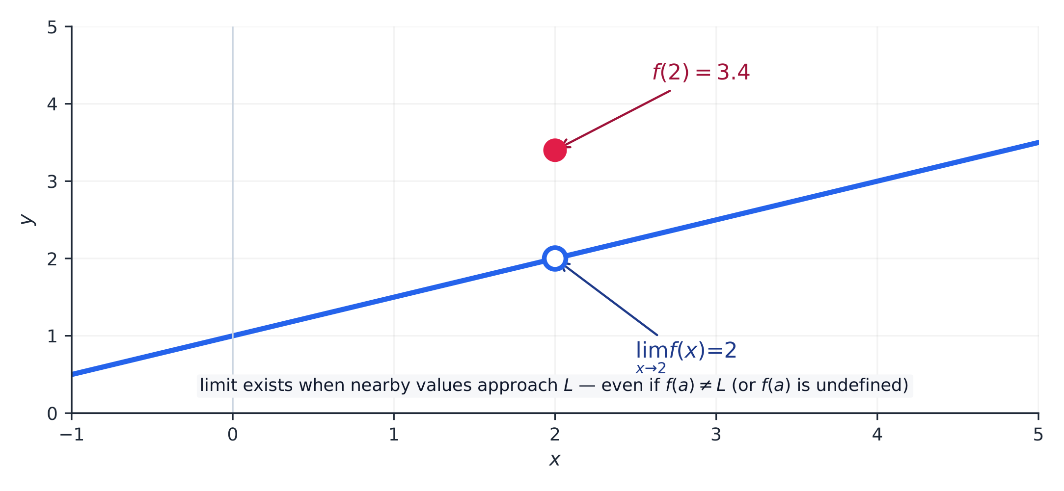
A graph is often the fastest way to read a limit. To find $\displaystyle \lim_{x \to c} f(x)$, run your finger along the curve toward $x = c$ from each side and ask: what height is the curve heading for?
- Trace from the left (inputs smaller than $c$): this gives the left-hand limit 左极限, $\displaystyle \lim_{x \to c^-} f(x)$.
- Trace from the right (inputs larger than $c$): this gives the right-hand limit 右极限, $\displaystyle \lim_{x \to c^+} f(x)$.
- These are the one-sided limits 单侧极限. If both head to the same height $R$, then the two-sided limit exists and $\displaystyle \lim_{x \to c} f(x) = R$.
Crucially, ignore the point itself. Graphs mark the difference between the limit and the value:
- An open circle 空心圆 marks a height the curve approaches but does not reach – a "hole" 空洞.
- A closed circle 实心圆 marks the actual value $f(c)$.
So a curve may approach $R = 3$ from both sides (limit is $3$) while a filled dot sits at height $5$ (value $f(c) = 5$). The limit is $3$; the two need not match.
The open circle is the height the curve approaches (the limit); the filled dot is the actual value $f(2)$ – they need not agree. A limit does not exist (often written DNE) when the two sides disagree (a jump 跳跃), when the function is unbounded 无界 (grows without limit), or when it oscillates 振荡 forever near $c$. For example:
$$\lim_{x \to 0} \frac{1}{x^2} = \infty, \qquad \lim_{x \to 0} \frac{|x|}{x}\ \text{DNE}, \qquad \lim_{x \to 0} \sin\!\left(\frac{1}{x}\right)\ \text{DNE}.$$Watch the scale 比例 of a graph: a zoomed-out picture can hide important behavior near a point, so confirm with algebra when you can.
탐색하기Read a limit off the graph
y = ax² + bx + c
The limit as $x\to c$ is the height the curve heads toward from both sides — it is about where the function is going, not its value at $c$. Follow the curve toward an $x$ and read the $y$ it approaches.
어휘 연습하기English 한국어 left-hand limit/left hænd ˈlɪmɪt/ 좌측 한계 right-hand limit/raɪt hænd ˈlɪmɪt/ 우측 한계 one-sided limits/wʌn ˈsaɪdɪd ˈlɪmɪts/ 일변한 극한 open circle/ˈəʊpən ˈsɜːkl/ 빈 원 closed circle/kləʊzd ˈsɜːkl/ 닫힌 원 jump/dʒʌmp/ 점프 unbounded/ʌnˈbaʊndɪd/ 무한대 oscillates/ˈɒsɪleɪts/ 진동한다 scale/skeɪl/ 스케일(scale) 1.4
Estimating Limit Values from Tables
Syllabus
지속적 이해(LIM-1): 정의, 정리, 성질을 이용한 추론을 통해 극한에 대한 주장을 정당화할 수 있습니다.
학습 목표 LIM-1.C: 함수의 극한을 추정합니다.
- LIM-1.C.5 수치 정보를 사용하여 극한을 추정할 수 있습니다.
출처: College Board AP Course and Exam Description
When you have data or a formula but no picture, a table 表格 of values estimates a limit numerically. Choose inputs that creep toward $c$ from both sides and watch the outputs.
For example, to estimate $\displaystyle \lim_{x \to 2} \frac{x^2 - 4}{x - 2}$ (which is $\tfrac{0}{0}$ at $x=2$):
$x$ $1.9$ $1.99$ $1.999$ $\to 2 \leftarrow$ $2.001$ $2.01$ $2.1$ $f(x)$ $3.9$ $3.99$ $3.999$ ? $4.001$ $4.01$ $4.1$ Both sides march toward $4$, so we estimate the limit is $4$. A table only suggests a value – it is a numerical estimate, not a proof.
어휘 연습하기English 한국어 table/ˈteɪbl/ 표 1.5
Determining Limits Using Algebraic Properties of Limits
Syllabus
지속적 이해(LIM-1): 정의, 정리, 성질을 이용한 추론을 통해 극한에 대한 주장을 정당화할 수 있습니다.
학습 목표 LIM-1.D: 극한 정리를 사용하여 함수의 극한을 결정합니다.
- LIM-1.D.1 양측 극한은 해석적 또는 기하적으로 결정할 수 있습니다.
- LIM-1.D.2 합, 차, 곱, 상, 합성함수의 극한은 극한 정리를 통해 구할 수 있습니다.
출처: College Board AP Course and Exam Description
Most limits are found analytically using limit theorems 极限定理. If $\lim_{x\to c} f(x)$ and $\lim_{x\to c} g(x)$ both exist, the limit of a combination is the same combination of the limits:
- Sum / difference: $\displaystyle \lim_{x\to c}\big[f(x)\pm g(x)\big] = \lim_{x\to c}f(x) \pm \lim_{x\to c}g(x)$
- Product: $\displaystyle \lim_{x\to c}\big[f(x)\,g(x)\big] = \lim_{x\to c}f(x)\cdot\lim_{x\to c}g(x)$
- Quotient: $\displaystyle \lim_{x\to c}\frac{f(x)}{g(x)} = \frac{\lim_{x\to c}f(x)}{\lim_{x\to c}g(x)}$, provided the bottom limit is not $0$.
- Composite 复合函数: if $g$ is continuous at $\lim_{x\to c} f(x)$, then $\displaystyle \lim_{x\to c} g\big(f(x)\big) = g\!\left(\lim_{x\to c} f(x)\right)$.
The practical rule: for a function built from polynomials, roots, and the like, first try direct substitution 直接代入 – put $x = c$ in. If you get a real number, that is the limit. One-sided limits obey the same theorems, read from one direction only.
어휘 연습하기English 한국어 limit theorems/ˈlɪmɪt ˈθɪərəmz/ 극한 정리 Composite/ˈkɒmpəzɪt/ 합성체 direct substitution/daɪˈrekt ˌsʌbstɪˈtjuːʃn/ 직접 치환 1.6
Determining Limits Using Algebraic Manipulation
Syllabus
지속적 이해(LIM-1): 정의, 정리, 성질을 이용한 추론을 통해 극한에 대한 주장을 정당화할 수 있습니다.
학습 목표 LIM-1.E: 함수의 등가 표현이나挟定理(Squeeze Theorem)을 사용하여 함수의 극한을 결정합니다.
- LIM-1.E.1 극한을 평가하기 전에 식을 등가 형태로 재배열해야 하거나 도움이 될 수 있습니다.
- LIM-1.E.1의 예시:
- 유리함수의 공통 인수를 인수분해하여 나누기
- 근호를 포함하는 함수를 단순화하기 위해 합이나 차의 켤레를 포함한 식을 곱하기
- 삼각함수의 대안적 형식 사용
- LIM-1.E.1의 예시:
출처: College Board AP Course and Exam Description
Direct substitution sometimes gives the indeterminate form 未定式 $\tfrac{0}{0}$. This does not mean the limit fails – it means you must rewrite the function into an equivalent form 等价形式 that removes the trouble, then substitute. Three standard moves:
- Factor and cancel 因式分解并约分 a rational function 有理函数. Example: $\displaystyle \lim_{x\to 2}\frac{x^2-4}{x-2} = \lim_{x\to 2}\frac{(x-2)(x+2)}{x-2} = \lim_{x\to 2}(x+2) = 4$.
- Multiply by the conjugate 共轭 to simplify a radical 根式. Example: $\displaystyle \lim_{x\to 0}\frac{\sqrt{x+1}-1}{x} = \lim_{x\to 0}\frac{x}{x\big(\sqrt{x+1}+1\big)} = \frac{1}{2}$.
- Use alternate forms of trigonometric functions (identities) to simplify.
The cancelled factor is why the original graph had a hole: the two functions agree everywhere except at $x=c$, so they share the same limit there.
어휘 연습하기English 한국어 indeterminate form/ˌɪndɪˈtɜːmɪnət fɔːm/ 부정정 형식 equivalent form/ɪˈkwɪvələnt fɔːm/ 등가 형태 Factor and cancel/ˈfæktə ænd ˈkænsl/ 인수분해 및 약분 rational function/ˈræʃənl ˈfʌŋkʃn/ 유계 함수 conjugate/ˈkɒndʒuːɡeɪt/ 상쇄 산/염기 radical/ˈrædɪkl/ 급진적 1.7
Selecting Procedures for Determining Limits
Syllabus
이 주제는 적절한 극한 결정 절차를 선택하는 기술에 집중하도록 설계되었습니다. 학생들은 극한 결정과 관련된 모든 학습 목표를 언제와 어떻게 적용할지 연습할 기회를 제공받아야 합니다.
출처: College Board AP Course and Exam Description
This is a skill topic, not new content: choose the right tool for the limit in front of you.
- Try direct substitution first. A real answer means you are done.
- Getting $\tfrac{0}{0}$? Rewrite – factor and cancel, or use the conjugate, or a trig identity – then substitute.
- A non-zero number over $0$ (like $\tfrac{5}{0}$)? The limit is infinite or DNE – check the sign from each side (see vertical asymptotes below).
- As $x\to\pm\infty$? Compare the dominant 主导 terms (see limits at infinity).
- Trapped between two functions? The squeeze theorem may apply.
어휘 연습하기English 한국어 dominant/ˈdɒmɪnənt/ 주요(dominant) 1.8
Determining Limits Using the Squeeze Theorem

Syllabus
지속적 이해(LIM-1): 정의, 정리, 성질을 이용한 추론을 통해 극한에 대한 주장을 정당화할 수 있습니다.
학습 목표 LIM-1.E: 함수의 등가 표현이나挟定理(Squeeze Theorem)을 사용하여 함수의 극한을 결정합니다.
- LIM-1.E.2 함수의 극한은挟定理를 사용하여 구할 수 있습니다.
- LIM-1.E.2의 예시: 挟定理를 사용하여 $\lim_{x \to 0} \dfrac{\sin x}{x} = 1$과 $\lim_{x \to 0} \dfrac{1 - \cos x}{x} = 0$임을 보여줄 수 있습니다.
출처: College Board AP Course and Exam Description
The squeeze theorem 夹逼定理 (also called the sandwich theorem) finds a limit by trapping the function between two others. If $g(x) \le f(x) \le h(x)$ near $c$, and
$$\lim_{x\to c} g(x) = \lim_{x\to c} h(x) = L,$$then $f$ is squeezed to the same place: $\displaystyle \lim_{x\to c} f(x) = L$.The two famous results proved this way, both used throughout calculus, are:
$$\lim_{x\to 0}\frac{\sin x}{x} = 1 \qquad\text{and}\qquad \lim_{x\to 0}\frac{1-\cos x}{x} = 0.$$The wiggly $f$ is trapped between $g$ and $h$. Because both bounds meet at $L$, $f$ has nowhere to go but $L$. 어휘 연습하기English 한국어 squeeze theorem/skwiːz ˈθɪərəm/ sandwich 정리 1.9
Connecting Multiple Representations of Limits
Syllabus
이 주제는 표현 방식 간의 연결에 집중하도록 설계되었습니다. 학생들은 극한과 관련된 모든 학습 목표를 언제와 어떻게 적용하고, 단일 표현 또는 여러 표현 간에 있는 수학 정보를 변환하는 법을 연습할 기회를 제공받아야 합니다.
출처: College Board AP Course and Exam Description
Another skill topic: the same limit lives in a graph, a table, and an algebraic form, and you should be able to translate between them. A graph shows the shape and any holes or jumps; a table gives numerical evidence; algebra gives an exact value and a reason. Strong answers use one representation to confirm another.
1.10
Exploring Types of Discontinuities
Syllabus
지속적 이해 (LIM-2): 정의, 정리, 성질을 활용한 추론을 통해 연속에 대한 주장을 정당화할 수 있다.
학습 목표 LIM-2.A: 정의에 근거하여 특정 점에서의 연속성에 대한 결론을 정당화한다.
- LIM-2.A.1 불연속의 종류로는 제거 가능한 불연속, 점프 불연속, 수직 asymptote로 인한 불연속이 포함된다.
출처: College Board AP Course and Exam Description
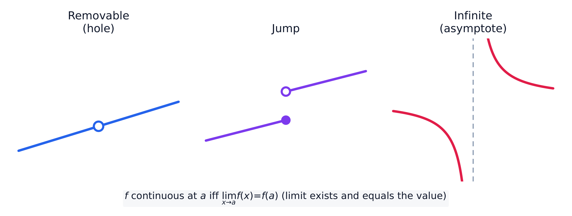
A function is discontinuous 间断 at $c$ when its graph "breaks" there. There are three types:
- Removable discontinuity 可去间断 – a single hole. The two-sided limit exists, but the point is missing or misplaced.
- Jump discontinuity 跳跃间断 – the two one-sided limits exist but disagree, so the curve jumps.
- Infinite discontinuity 无穷间断 – the function blows up to $\pm\infty$ at a vertical asymptote 垂直渐近线.
Three ways a graph can break: a removable hole, a jump, and an infinite (asymptote) discontinuity. 어휘 연습하기English 한국어 discontinuous/dɪskənˈtɪnjuːəs/ 불연속적 Removable discontinuity/rɪˈmuːvəbl dɪskɒntɪˈnjuːɪti/ 제거 가능한 불연속점 Jump discontinuity/dʒʌmp dɪskɒntɪˈnjuːɪti/ 약점 불연속점 Infinite discontinuity/ˈɪnfɪnət dɪskɒntɪˈnjuːɪti/ 무한 불연속점 vertical asymptote/ˈvɜːtɪkl ˈæsɪmptəʊt/ 수직 점근선 1.11
Defining Continuity at a Point
Syllabus
지속적 이해 (LIM-2): 정의, 정리, 성질을 활용한 추론을 통해 연속에 대한 주장을 정당화할 수 있다.
학습 목표 LIM-2.A: 정의에 근거하여 특정 점에서의 연속성에 대한 결론을 정당화한다.
- LIM-2.A.2 함수 $f$가 $x = c$에서 연속이 되기 위해서는 $f(c)$가 존재하고, $\lim_{x \to c} f(x)$가 존재하며, $\lim_{x \to c} f(x) = f(c)$이어야 한다.
출처: College Board AP Course and Exam Description
Continuity is defined by a three-part test. A function $f$ is continuous 连续 at $x=c$ exactly when all three hold:
$$\boxed{\;f(c)\text{ exists}\quad\text{and}\quad \lim_{x\to c} f(x)\text{ exists}\quad\text{and}\quad \lim_{x\to c} f(x) = f(c)\;}$$In words: the point is there, the limit is there, and the two agree. If any one fails, $f$ is discontinuous at $c$. This test is the backbone of nearly every continuity question, so learn it as a checklist.
어휘 연습하기English 한국어 continuous/kənˈtɪnjuːəs/ 연속적 1.12
Confirming Continuity over an Interval
Syllabus
지속적 이해 (LIM-2): 정의, 정리, 성질을 활용한 추론을 통해 연속에 대한 주장을 정당화할 수 있다.
학습 목표 LIM-2.B: 함수가 연속인 구間을 결정한다.
- LIM-2.B.1 함수가 어떤 구간의 모든 점에서 연속이라면, 그 구간 전체에서 연속이라고 한다.
- LIM-2.B.2 다항함수,有理함수, 지수함수, 로그함수, 삼각함수는 도메인 내 모든 점에서 연속이다.
출처: College Board AP Course and Exam Description
A function is continuous on an interval 在区间上连续 if it is continuous at every point of that interval. You rarely check point by point, because whole families are continuous on their domains:
Polynomial, rational, power, exponential 指数, logarithmic 对数, and trigonometric 三角 functions are continuous at every point of their domains.
So a rational function is continuous everywhere except where its denominator is zero; $\ln x$ is continuous for $x>0$; and so on. Knowing this lets you declare continuity quickly and correctly.
어휘 연습하기English 한국어 continuous on an interval/kənˈtɪnjuːəs ɒn ən ˈɪntəvl/ 구간에 대해 연속함 exponential/ˌekspəˈnenʃl/ 지수Unless exponential function. logarithmic/ˌlɒɡəˈrɪθmɪk/ 로그함수 trigonometric/ˌtrɪɡənəʊˈmetrɪk/ 삼각함수 1.13
Removing Discontinuities
Syllabus
지속적 이해 (LIM-2): 정의, 정리, 성질을 활용한 추론을 통해 연속에 대한 주장을 정당화할 수 있다.
학습 목표 LIM-2.C: $x$의 값을 결정하거나, 불연속인 함수를 연속으로 만들 수 있는 매개변수를 구한다(가능할 경우).
- LIM-2.C.1 함수의 그래프 상에서 불연속점에서의 함수의 극한이 존재할 경우, 그 점에서의 함수 값을 정의하거나 재정의하여 극한의 값과 같게 함으로써 불연속성을 제거할 수 있다. 이때 $x$이 그 점에 접근할 때의 함수의 극한 값과 같아진다.
- LIM-2.C.2分区-defined 함수가 도메인 partition의 경계에서 연속이 되려면, 경계의 한 측면을 정의하는 식의 값이 다른 측면을 정의하는 식의 값 및 경계에서의 함수 값과 모두 같아야 한다.
출처: College Board AP Course and Exam Description
If the limit exists at a hole, the discontinuity is removable: redefine the function at that one point to equal the limit, and the graph is repaired. Formally, set the missing value to $\displaystyle \lim_{x\to c} f(x)$.
For a piecewise-defined function 分段函数, continuity at a boundary $x=c$ needs the two pieces to meet: the left piece's value, the right piece's value, and $f(c)$ must all be equal. This is a common exam setup – you solve for a parameter 参数 (an unknown constant) that makes the pieces match:
$$\lim_{x\to c^-} f(x) = \lim_{x\to c^+} f(x) = f(c).$$어휘 연습하기English 한국어 piecewise-defined function/ˈpiːswaɪz dɪˈfaɪnd ˈfʌŋkʃn/ 부분 정의 함수 parameter/pəˈræmɪtə/ 파라미터 1.14
Connecting Infinite Limits and Vertical Asymptotes
Syllabus
지속적 이해 (LIM-2): 정의, 정리, 성질을 활용한 추론을 통해 연속에 대한 주장을 정당화할 수 있다.
학습 목표 LIM-2.D: 무한을 포함한 극한을 사용하여 함수의 거동을 해석한다.
- LIM-2.D.1 극한의 개념은 무한극한을 포함하도록 확장될 수 있다.
- LIM-2.D.2 함수의 점근적 거동 및 비유계 거동은 극한을 사용하여 설명하고 해석할 수 있다.
출처: College Board AP Course and Exam Description
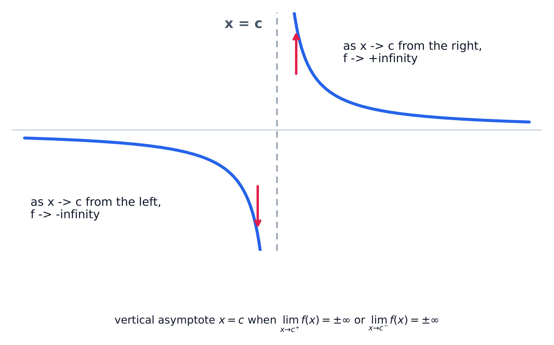
The idea of a limit extends to infinite limits 无穷极限. When a function grows without bound near $x=c$, we write $\lim_{x\to c} f(x) = \pm\infty$. This describes a vertical asymptote at $x=c$: the graph hugs the vertical line $x=c$ and shoots off toward $\pm\infty$.
This happens where a non-zero number is divided by something approaching $0$, such as at a zero of a denominator that does not cancel. Always check each side separately – the two sides can shoot opposite ways (one to $+\infty$, one to $-\infty$).
Near a vertical asymptote the graph hugs the line $x=c$. Here the left side falls to $-\infty$ and the right side climbs to $+\infty$, so the two-sided limit does not exist. 탐색하기Explore infinite limits and vertical asymptotes
y = a/(x − b) + c
With $y=\dfrac{a}{x-b}+c$, watch the curve blow up to $\pm\infty$ near $x=b$. The vertical asymptote is the line $x=b$ where the infinite limit lives — the two sides can shoot opposite ways.
어휘 연습하기English 한국어 infinite limits/ˈɪnfɪnət ˈlɪmɪts/ 무한 극한 1.15
Connecting Limits at Infinity and Horizontal Asymptotes
Syllabus
지속적 이해 (LIM-2): 정의, 정리, 성질을 활용한 추론을 통해 연속에 대한 주장을 정당화할 수 있다.
학습 목표 LIM-2.D: 무한을 포함한 극한을 사용하여 함수의 거동을 해석한다.
- LIM-2.D.3 극한의 개념은 무한에서의 극한을 포함하도록 확장될 수 있다.
- LIM-2.D.4 무한에서의 극한은 끝행동을 설명합니다.
- LIM-2.D.5 함수와 그 변화율의 상대적 크기는 극한을 사용하여 비교할 수 있습니다.
출처: College Board AP Course and Exam Description
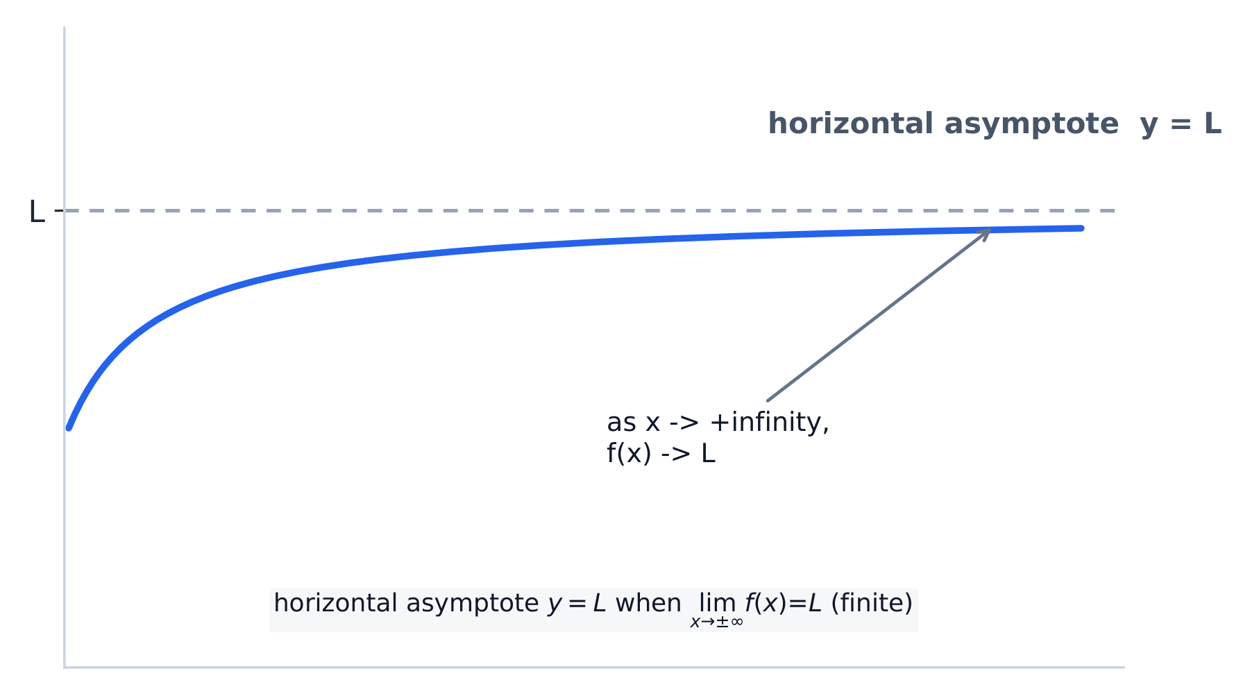
We can also let the input grow: limits at infinity 无穷远处的极限 describe the end behavior 末端行为 of a function as $x\to\pm\infty$. If the outputs settle toward a finite value $L$, then $y=L$ is a horizontal asymptote 水平渐近线.
As $x\to+\infty$ the curve flattens toward the line $y=L$. The horizontal asymptote records this end behavior. For a rational function, compare the degrees 次数 of the top and bottom:
- top degree < bottom degree $\Rightarrow$ limit is $0$ (asymptote $y=0$);
- top degree = bottom degree $\Rightarrow$ limit is the ratio of the leading coefficients 首项系数之比;
- top degree > bottom degree $\Rightarrow$ the function is unbounded (no horizontal asymptote).
More generally, we compare the relative magnitudes 相对大小 (relative growth rates) of functions: far out, an exponential beats any polynomial, and a polynomial beats any logarithm. On the exam, "as $t\to\infty$, which quantity is larger/where does the rate settle?" is answered with a limit at infinity.
탐색하기Explore limits at infinity and horizontal asymptotes
y = a/(x − b) + c
Follow the curve far out to the right and left. As $x\to\pm\infty$ the outputs settle toward $c$, so $y=c$ is a horizontal asymptote — the finite value of the limit at infinity.
어휘 연습하기English 한국어 limits at infinity/ˈlɪmɪts æt ɪnˈfɪnɪti/ 무한에서의 한계 end behavior/end bɪˈheɪvjə/ 말단挙動 horizontal asymptote/ˌhɒrɪˈzɒntl ˈæsɪmptəʊt/ 수평 점근선 degrees/dɪˈɡriːz/ 도 ratio of the leading coefficients/ˈreɪʃɪəʊ ɒvðə ˈliːdɪŋ ˌkəʊɪˈfɪʃənts/ 최고차 계수의 비율 relative magnitudes/ˈrelətɪv ˈmæɡnɪtjuːdz/ 상대 크기 1.16
Working with the Intermediate Value Theorem (IVT)
Syllabus
지속적 이해(FUN-1): 존재 정리는 특정 구간에서 함수의 행동을 정확히 locating하지 않고도 결론을 내릴 수 있게 해줍니다.
학습 목표 FUN-1.A: 중간값 정리를 사용하여 한 구간에서 함수의 행동을 설명합니다.
- FUN-1.A.1 $f$가 닫힌 구간 $[a, b]$에서 연속인 함수이고, $d$가 $f(a)$와 $f(b)$ 사이의 실수라면, 중간값 정리는 적어도 하나의 숫자 $c$이 $a$과 $b$ 사이에 존재하여 $f(c) = d$이 성립함을 보장합니다.
출처: College Board AP Course and Exam Description
The Intermediate Value Theorem 介值定理 is an existence theorem 存在性定理 – it guarantees a value exists without telling you where:
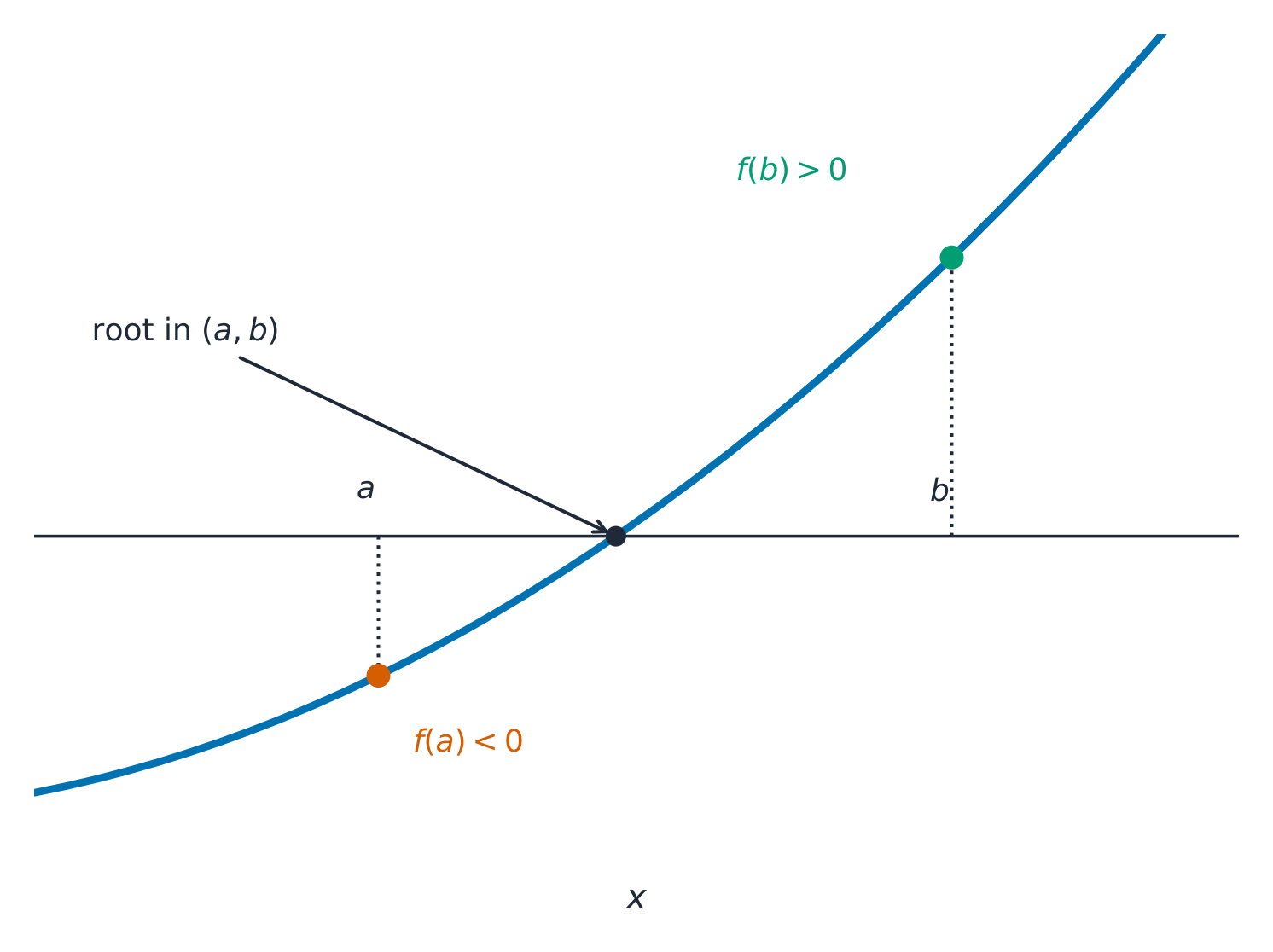
Opposite signs of f(a) and f(b) trap a root between a and b If $f$ is continuous on the closed interval $[a,b]$, and $d$ is any number between $f(a)$ and $f(b)$, then there is at least one number $c$ in $(a,b)$ with $f(c)=d$.
An unbroken curve cannot skip a height between its endpoints – it must pass through every one.
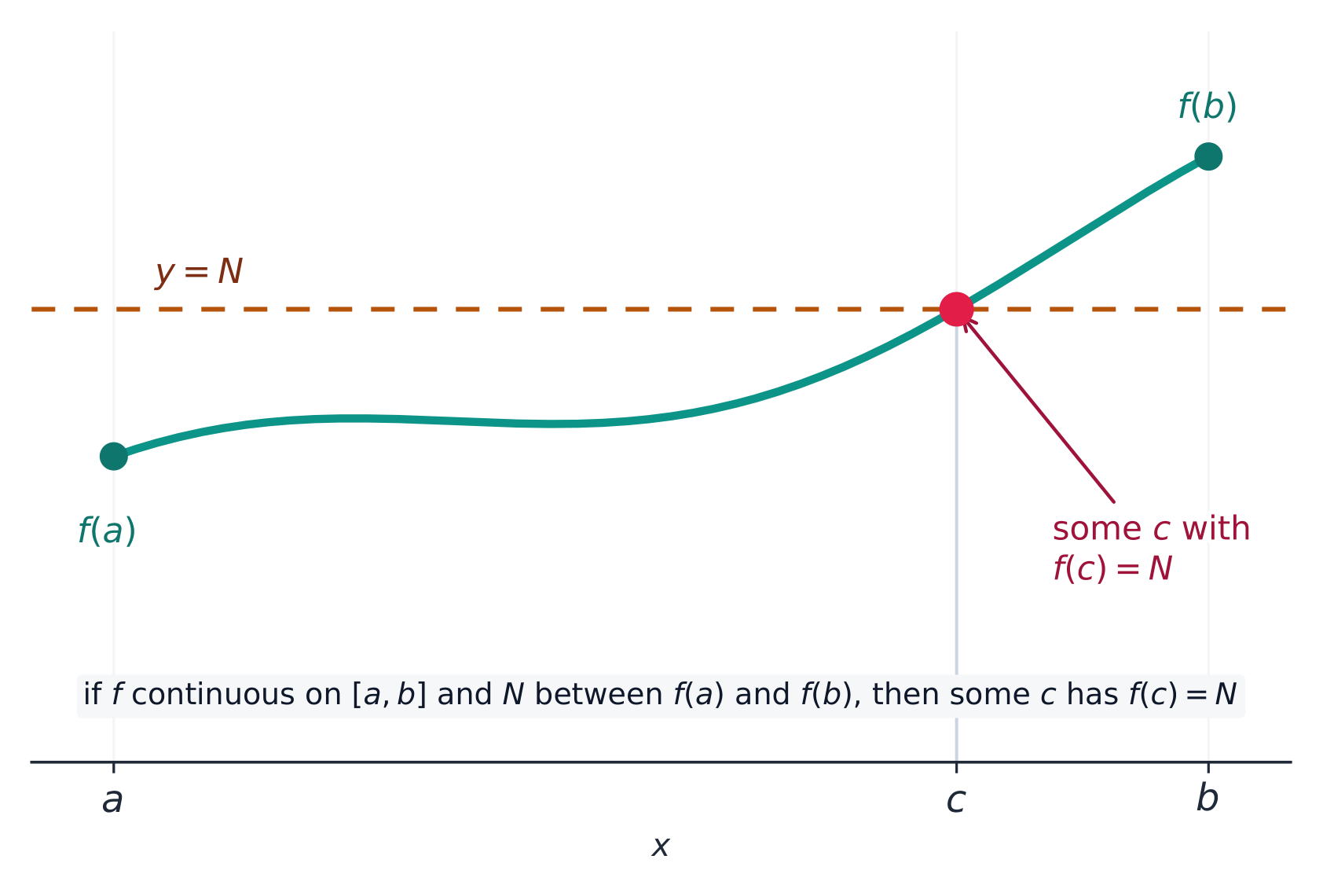
A continuous curve from $(a,f(a))$ to $(b,f(b))$ must cross every height $d$ in between at least once. Exam skill – how to justify with the IVT. These questions appear almost every year (for example, "Must there be a value $c$ with $R(c)=155$?" or "Is there a time when $r'(t)=-6$?"). A full-credit justification has three moves:
- State continuity. Say the function is continuous on $[a,b]$ (often because it is differentiable, or given continuous).
- Show $d$ is trapped. Compute the two endpoint values and show the target $d$ lies between them, e.g. $f(a) < d < f(b)$.
- Conclude by name. "By the Intermediate Value Theorem, there is a $c$ in $(a,b)$ with $f(c)=d$."
Skipping the continuity statement, or not showing $d$ is between the endpoints, loses the point – the theorem requires both conditions.
Worked example. Evaluate $\lim_{x\to 3}\dfrac{x^2-9}{x-3}$. Direct substitution gives $\tfrac{0}{0}$ (indeterminate), so factor: $\dfrac{(x-3)(x+3)}{x-3}=x+3$ for $x\ne 3$. Then $\lim_{x\to 3}(x+3)=6$. The graph has a removable discontinuity (a hole) at $x=3$ — the limit exists even though the function is undefined there.
탐색하기Why a continuous curve can't skip a value
y = ax³ + bx² + cx + d
The Intermediate Value Theorem: a function continuous on $[a,b]$ takes every $y$ between $f(a)$ and $f(b)$ at some point inside. An unbroken curve cannot leap over a height — it must pass through it.
어휘 연습하기English 한국어 Intermediate Value Theorem/ˌɪntəˈmiːdɪət ˈvæljuː ˈθɪərəm/ 중간값 정리 existence theorem/eɡˈzɪstəns ˈθɪərəm/ 존재 정리 1.16
Exam tips
- A limit describes what $f(x)$ approaches, which need not equal $f(a)$ — the two-sided limit exists only if both sides agree.
- Try direct substitution first; for a $\tfrac00$ form, factor and cancel or rationalise before substituting.
- A function is continuous at $a$ when the limit exists, $f(a)$ is defined, and they are equal.
- Use the Intermediate Value Theorem to guarantee a root: a continuous function that changes sign on $[a,b]$ takes every value between.
- Read horizontal asymptotes from end behaviour (limits at $\pm\infty$) and vertical asymptotes where the denominator (not the numerator) is zero.
-
2
미분: 정의 및 기본 성질
수업 보기2.1
Average and Instantaneous Rates of Change
Syllabus
지속적 이해 (CHA-2): 미분은 구간 내의 변화율에 대한 지식을 극한에 적용함으로써 순간의 변화율을 결정할 수 있게 해줍니다.
학습 목표 CHA-2.A: 차분商(difference quotients)을 사용하여 평균 변화율을 결정합니다.
- CHA-2.A.1 차분商 $\dfrac{f(a+h)-f(a)}{h}$과 $\dfrac{f(x)-f(a)}{x-a}$은 한 구간에서 함수의 평균 변화율을 나타냅니다.
학습 목표 CHA-2.B: 함수의 미분을 차분商의 극한으로 표현합니다.
- CHA-2.B.1 함수의 $x=a$에서의 순간 변화율은 극한이 존재할 때 $\lim\limits_{h\to 0}\dfrac{f(a+h)-f(a)}{h}$ 또는 $\lim\limits_{x\to a}\dfrac{f(x)-f(a)}{x-a}$로 표현할 수 있습니다. 이들은 미분의 정의의 등가 형태이며 $f'(a)$로 표시됩니다.
출처: College Board AP Course and Exam Description
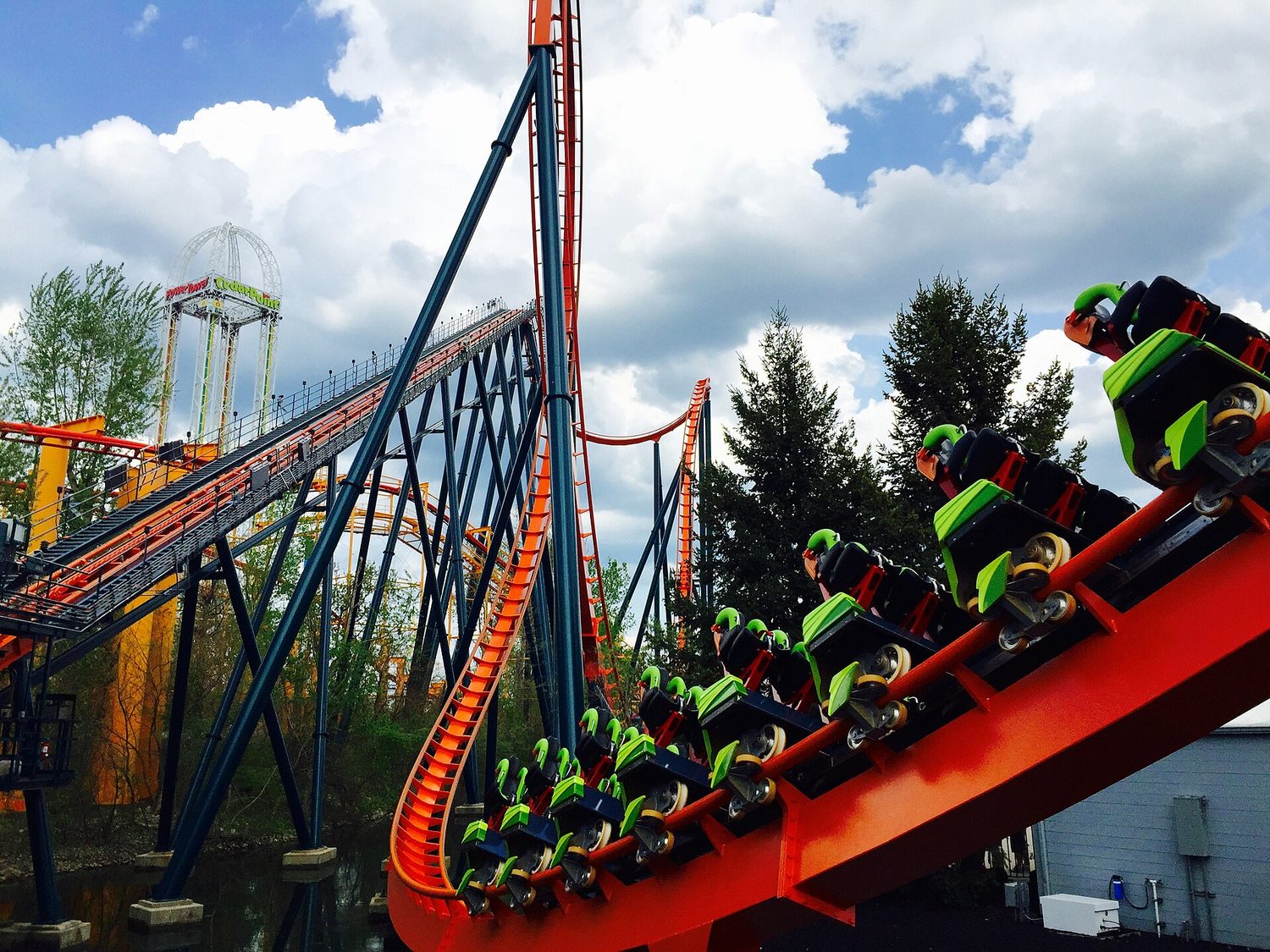
A roller coaster on a lift hill: the derivative measures instantaneous rate of change of position The derivative from first principles Unit 1 built the limit. Unit 2 uses it to define the derivative 导数 – the exact rate of change at a point.
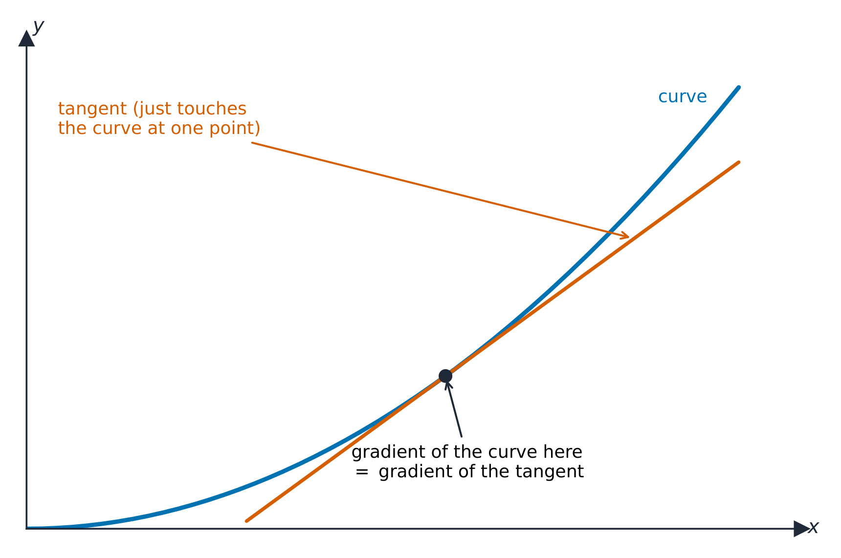
The instantaneous rate of change is the gradient of the tangent at a point Over an interval, the average rate of change is a difference quotient 差商. Two equivalent forms appear:
$$\frac{f(a+h)-f(a)}{h} \qquad\text{and}\qquad \frac{f(x)-f(a)}{x-a}.$$The first uses a step of size $h$ from $a$; the second uses two points $x$ and $a$. Both compute $\dfrac{\text{change in output}}{\text{change in input}}$ over the interval.The instantaneous 瞬时 rate of change at $x=a$ is what the difference quotient approaches as the interval shrinks to zero. This limit is the derivative at $a$, written $f'(a)$:
$$f'(a) = \lim_{h\to 0}\frac{f(a+h)-f(a)}{h} = \lim_{x\to a}\frac{f(x)-f(a)}{x-a},$$provided the limit exists.탐색하기From average rate to instantaneous rate
y = ax³ + bx² + cx + d
Slide the point: the secant through two nearby points tips toward the tangent as they merge. The tangent's slope is the derivative — the instantaneous rate of change.
어휘 연습하기English 한국어 derivative/dɪˈrɪvətɪv/ 미분Unless derivative. difference quotient/ˈdɪfrəns ˈkwəʊʃənt/ 차분 비 instantaneous/ˌɪnstənˈteɪnɪəs/ 순간 first principles/fɜːst ˈprɪnsɪplz/ 기본 원리 2.2
Defining the Derivative and Its Notation
Syllabus
지속적 이해 (CHA-2): 미분은 구간 내의 변화율에 대한 지식을 극한에 적용함으로써 순간의 변화율을 결정할 수 있게 해줍니다.
학습 목표 CHA-2.B: 함수의 미분을 차분商의 극한으로 표현합니다.
- CHA-2.B.2 $f$의 미분은 극한이 존재할 때 $x$에서의 값이 $\lim\limits_{h\to 0}\dfrac{f(x+h)-f(x)}{h}$인 함수입니다.
- CHA-2.B.3 $y=f(x)$에 대한 미분 표기법에는 $\dfrac{dy}{dx}$, $f'(x)$, $y'$이 포함됩니다.
- CHA-2.B.4 미분은 기하학적, 수치적, 해석적, 서술적으로 표현될 수 있습니다.
학습 목표 CHA-2.C: 주어진 점에서 곡선에 접선인 직선의 방정식을 결정합니다.
- CHA-2.C.1 점에서의 함수의 미분은 해당 점에서의 함수 그래프에 접선인 직선의 기울기입니다.
출처: College Board AP Course and Exam Description
Let the point $a$ vary and the derivative becomes a new function:
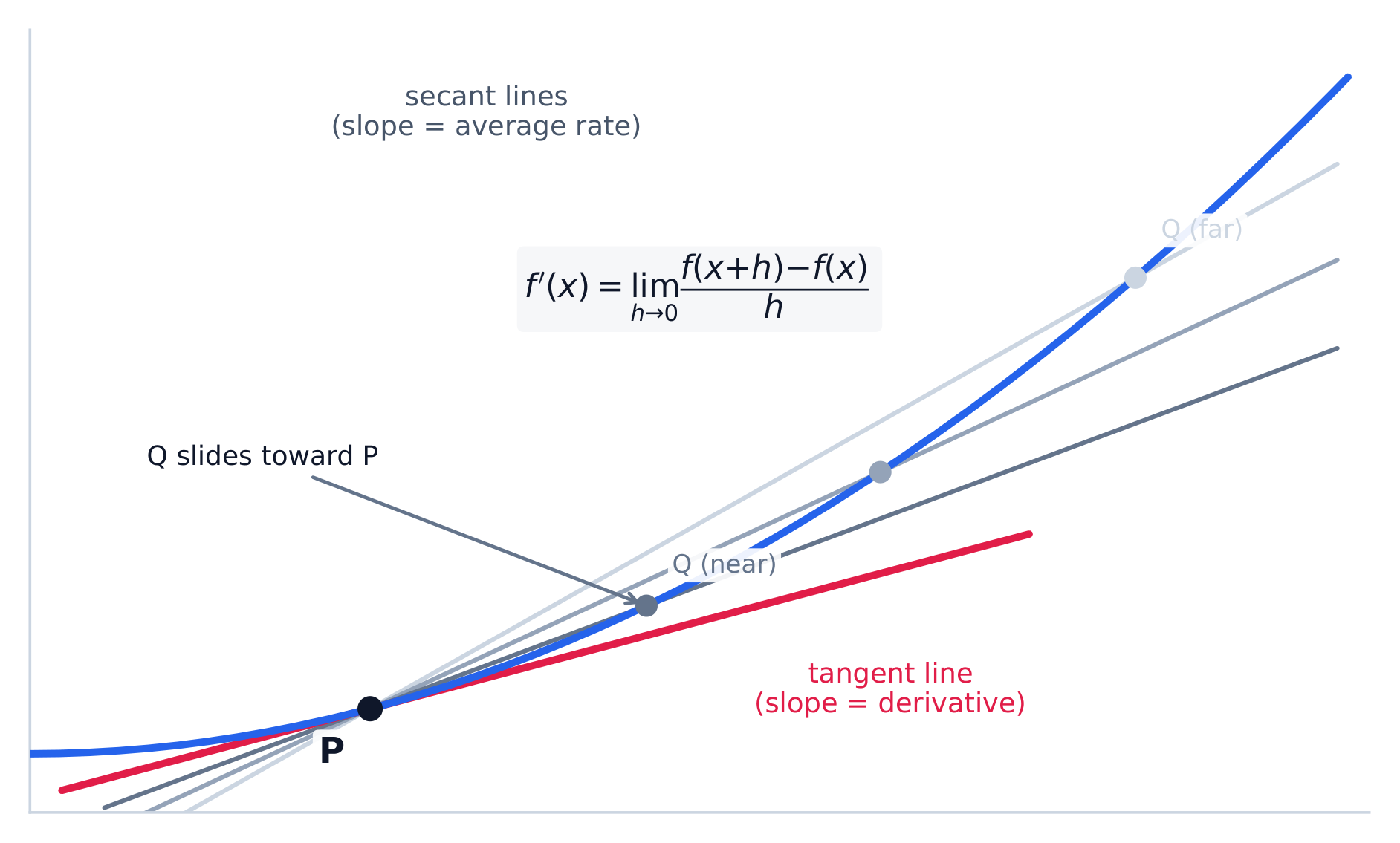
$$f'(x) = \lim_{h\to 0}\frac{f(x+h)-f(x)}{h}.$$This is the definition of the derivative (sometimes called differentiating "by first principles" 用定义求导). Its value at each $x$ is the instantaneous rate of change there.Common notations 记号 for the derivative of $y=f(x)$ are:
$$\frac{dy}{dx}, \qquad f'(x), \qquad y'.$$The derivative can be represented graphically, numerically, analytically, and verbally – be ready to move between them.Geometric meaning. The derivative at a point is the slope 斜率 of the tangent line 切线 to the graph there. So the tangent line at $x=a$ passes through $\big(a, f(a)\big)$ with slope $f'(a)$:
$$y - f(a) = f'(a)\,(x-a).$$Writing this line is a routine exam task, so keep the point-slope form ready.As $Q$ slides toward $P$, each secant's slope (an average rate) approaches the tangent's slope – the derivative $f'(a)$. 어휘 연습하기English 한국어 notations/nəʊˈteɪʃnz/ 표기법 slope/sləʊp/ 기울기 tangent line/ˈtændʒənt laɪn/ 접선 2.3
Estimating a Derivative at a Point
Syllabus
지속적 이해 (CHA-2): 미분은 구간 내의 변화율에 대한 지식을 극한에 적용함으로써 순간의 변화율을 결정할 수 있게 해줍니다.
학습 목표 CHA-2.D: 도함수를 추정합니다.
- CHA-2.D.1 표나 그래프에 제공된 정보에서 점에서의 도함수를 추정할 수 있습니다.
- CHA-2.D.2 기술을 사용하여 점에서의 함수의 도함수 값을 계산하거나 추정할 수 있습니다.
출처: College Board AP Course and Exam Description
You do not always have a formula. When a function is given by a table 表格 or a graph, estimate the derivative $f'(a)$ with a difference quotient over a small interval around $a$. A table with values on both sides of $a$ gives the best estimate:
$$f'(a) \approx \frac{f(b)-f(c)}{b-c},\qquad \text{where } c < a < b \text{ are the closest table inputs}.$$Technology (a calculator) can also estimate a derivative at a point.Exam skill (appears almost every year). Questions such as "Approximate $M'(7.5)$ using the average rate of change of $M$ over the interval $5 \le t \le 10$" ask for exactly this difference quotient. Show the setup:
$$M'(7.5) \approx \frac{M(10)-M(5)}{10-5}.$$Full credit needs the numbers plugged in and the correct units 单位 (output units per input unit), since these come from real-world models.어휘 연습하기English 한국어 table/ˈteɪbl/ 표 units/ˈjuːnɪts/ 단위 2.4
When Does a Derivative Exist?
Syllabus
지속적 이해 (FUN-2): 함수의 미분도 하나의 함수일 수 있음을 인식하면 두 함수의 관련된 행동에 대한 지식을 개발할 수 있습니다.
학습 목표 FUN-2.A: 가미분 가능성과 연속성 사이의 관계를 설명합니다.
- FUN-2.A.1 함수가 한 점에서 가미분 가능하면 그 점에서 연속입니다. 특히, $f$의 정의역에 없는 점은 $f'$의 정의역에도 없습니다.
- FUN-2.A.2 연속 함수라도 정의역 내의 한 점에서 가미분 불가능할 수 있습니다.
- FUN-2.A.2의 예시:
- 차분商의 좌극한과 우극한이 서로 다른 경우, 예를 들어 $f(x)=|x|$에서 $x=0$인 경우
- 접선이 수직이고 기울기가 없는 경우, 예를 들어 $f(x)=\sqrt[3]{x}$에서 $x=0$인 경우
- FUN-2.A.2의 예시:
출처: College Board AP Course and Exam Description
Differentiability is stronger than continuity. The key relationship:
If $f$ is differentiable 可导 at a point, then $f$ is continuous 连续 there.
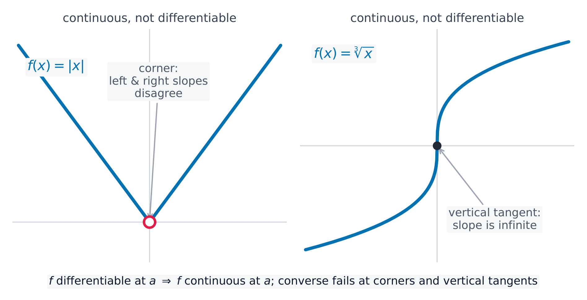
So differentiability implies continuity. The reverse is false: a continuous function can fail to be differentiable. Two ways this happens:
- A corner 尖点: the left and right difference-quotient limits disagree, as with $f(x)=|x|$ at $x=0$.
- A vertical tangent 垂直切线: the slope is infinite (no real number), as with $f(x)=\sqrt[3]{x}$ at $x=0$.
Two ways a continuous function is not differentiable: a corner and a vertical tangent Also, a point outside the domain of $f$ cannot be in the domain of $f'$. Use the contrapositive on the exam: if $f$ is not continuous at $a$, then $f$ is not differentiable at $a$.
어휘 연습하기English 한국어 differentiable/ˈdɪfərenʃɪəbl/ 미분 가능해야 함 continuous/kənˈtɪnjuːəs/ 연속적 corner/ˈkɔːnə/ 모서리 vertical tangent/ˈvɜːtɪkl ˈtændʒənt/ 수직 접선 2.5
The Power Rule
Syllabus
지속적 이해 (FUN-3): 미분 규칙을 적용할 수 있는 상황을 파악하면 미분 과정이 단순화됩니다.
학습 목표 FUN-3.A: 친숙한 함수의 도함수를 계산합니다.
- FUN-3.A.1 미분의 정의와 특정 규칙을 직접 적용하여 $f(x)=x^{r}$ 형태의 함수에 대한 미분값을 계산할 수 있다.
출처: College Board AP Course and Exam Description
From here we use rules instead of the limit definition each time. The power rule 幂法则 handles any power of $x$:
$$\frac{d}{dx}\,x^{r} = r\,x^{\,r-1}\qquad\text{for any real } r.$$It works for whole-number powers, negative powers ($\tfrac{1}{x}=x^{-1}$), and roots ($\sqrt{x}=x^{1/2}$) – rewrite as a power first, then apply the rule.탐색하기A power function and its steepening slope
y = ax³ + bx² + cx + d
The power rule $\frac{d}{dx}x^n = nx^{n-1}$ drops the exponent as a factor. For $x^3$ the slope grows quickly as $x$ moves from 0 — the curve steepens.
어휘 연습하기English 한국어 power rule/ˈpaʊə ruːl/ 거듭제곱 법칙 2.6
Constant, Sum, Difference, and Constant Multiple Rules
Syllabus
지속적 이해 (FUN-3): 미분 규칙을 적용할 수 있는 상황을 파악하면 미분 과정이 단순화됩니다.
학습 목표 FUN-3.A: 친숙한 함수의 도함수를 계산합니다.
- FUN-3.A.2 함수의 합, 차이 및 상수배는 미분 규칙을 사용하여 미분할 수 있다.
- FUN-3.A.3 지수 법칙을 합, 차이 및 상수배의 성질과 결합하여 다항함수에 대한 미분값을 구할 수 있다.
출처: College Board AP Course and Exam Description
These rules let you differentiate term by term:
- Constant: $\dfrac{d}{dx}\,k = 0$ (a constant does not change).
- Constant multiple 常数倍: $\dfrac{d}{dx}\big[k\,f(x)\big] = k\,f'(x)$.
- Sum / difference: $\dfrac{d}{dx}\big[f(x)\pm g(x)\big] = f'(x)\pm g'(x)$.
Combined with the power rule, they differentiate any polynomial 多项式 term by term. Example:
$$\frac{d}{dx}\big(4x^3 - 5x + 7\big) = 12x^2 - 5.$$어휘 연습하기English 한국어 Constant multiple/ˈkɒnstənt ˈmʌltɪpl/ 상수 곱 polynomial/ˌpɒlɪˈnəʊmɪəl/ 다항함수 2.7
Derivatives of sin x, cos x, e^x, and ln x
Syllabus
지속적 이해 (FUN-3): 미분 규칙을 적용할 수 있는 상황을 파악하면 미분 과정이 단순화됩니다.
학습 목표 FUN-3.A: 친숙한 함수의 도함수를 계산합니다.
- FUN-3.A.4 특정 규칙을 사용하여 삼각함수, 지수함수, 로그함수의 미분값을 구할 수 있다.
지속적 이해 (LIM-3): 정의, 정리, 성질을 이용한 추론으로 극한을 결정할 수 있다.
학습 목표 LIM-3.A: 미분의 정의로서 극함을 해석한다.
- LIM-3.A.1 일부 경우, 미분값이 알려진 함수의 미분 정의 식을 인식하는 것이 극한을 결정하기 위한 전략이 될 수 있다.
출처: College Board AP Course and Exam Description
Learn these four building-block derivatives by heart:
$$\frac{d}{dx}\sin x = \cos x, \qquad \frac{d}{dx}\cos x = -\sin x,$$$$\frac{d}{dx}e^{x} = e^{x}, \qquad \frac{d}{dx}\ln x = \frac{1}{x}\ \ (x>0).$$Note the minus sign on the derivative of cosine, and that $e^{x}$ is its own derivative.A limit that is really a derivative (LIM-3.A.1). Sometimes a limit is secretly the definition of a known derivative. If you recognize
$$\lim_{h\to 0}\frac{f(a+h)-f(a)}{h}$$for a function $f$ whose derivative you know, just evaluate $f'(a)$. For example, $\displaystyle \lim_{h\to 0}\frac{\sin\!\big(\tfrac{\pi}{2}+h\big)-1}{h} = \left.\frac{d}{dx}\sin x\right|_{x=\pi/2} = \cos\tfrac{\pi}{2} = 0$.탐색하기The shape of sin x (whose slope is cos x)
y = asin(bx + c) + d
The derivative of $\sin x$ is $\cos x$: the slope of the sine curve is largest where sine crosses zero and zero at its peaks. Watch the curve to feel where its slope is steep or flat.
2.8
The Product Rule
Syllabus
지속적 이해 (FUN-3): 미분 규칙을 적용할 수 있는 상황을 파악하면 미분 과정이 단순화됩니다.
학습 목표 FUN-3.B: 가미분 가능한 함수의 곱과 상의 도함수를 계산합니다.
- FUN-3.B.1 가미분 가능한 함수의 곱에 대한 미분값은 곱의 미분법을 통해 구할 수 있다.
출처: College Board AP Course and Exam Description
The product rule as a growing rectangle A product of two functions is not differentiated by multiplying the derivatives. Use the product rule 乘积法则:
$$\frac{d}{dx}\big[u\,v\big] = u'v + uv'.$$"Derivative of the first times the second, plus the first times the derivative of the second." Example:$$\frac{d}{dx}\big(x^2 e^{x}\big) = 2x\,e^{x} + x^2 e^{x}.$$Exam questions often build a new function from given pieces, e.g. $k'(x) = \big(f(x)\big)^2 g(x)$, and ask you to combine rules while reading values from a table.어휘 연습하기English 한국어 product rule/ˈprɒdʌkt ruːl/ 곱의 법칙 2.9
The Quotient Rule
Syllabus
지속적 이해 (FUN-3): 미분 규칙을 적용할 수 있는 상황을 파악하면 미분 과정이 단순화됩니다.
학습 목표 FUN-3.B: 가미분 가능한 함수의 곱과 상의 도함수를 계산합니다.
- FUN-3.B.2 가미분 가능한 함수의商에 대한 미분값은商的 미분법을 통해 구할 수 있다.
출처: College Board AP Course and Exam Description
For a quotient, use the quotient rule 商法则:
$$\frac{d}{dx}\!\left[\frac{u}{v}\right] = \frac{u'v - uv'}{v^{2}}.$$"Bottom times derivative of top, minus top times derivative of bottom, all over bottom squared." The order matters because of the minus sign, so write the numerator carefully. Example:$$\frac{d}{dx}\!\left(\frac{x}{\cos x}\right) = \frac{1\cdot\cos x - x\cdot(-\sin x)}{\cos^2 x} = \frac{\cos x + x\sin x}{\cos^2 x}.$$어휘 연습하기English 한국어 quotient rule/ˈkwəʊʃənt ruːl/ 비율의 법칙 2.10
Derivatives of tan x, cot x, sec x, and csc x
Syllabus
지속적 이해 (FUN-3): 미분 규칙을 적용할 수 있는 상황을 파악하면 미분 과정이 단순화됩니다.
학습 목표 FUN-3.B: 가미분 가능한 함수의 곱과 상의 도함수를 계산합니다.
- FUN-3.B.3 항등식을 사용하여 탄젠트, 코탄젠트, 섹cant, 코섹ant 함수를 재배열하면 미분 규칙을 사용하여 미분할 수 있습니다.
출처: College Board AP Course and Exam Description
The quotient rule: differentiating a fraction The remaining trigonometric derivatives are not memorized separately – you rewrite them with identities 恒等式 and apply the quotient (or product) rule. For instance, $\tan x = \dfrac{\sin x}{\cos x}$, so the quotient rule gives
$$\frac{d}{dx}\tan x = \frac{\cos x\cos x - \sin x(-\sin x)}{\cos^2 x} = \frac{1}{\cos^2 x} = \sec^2 x.$$The same method (writing $\cot x=\tfrac{\cos x}{\sin x}$, $\sec x=\tfrac{1}{\cos x}$, $\csc x=\tfrac{1}{\sin x}$) gives $-\csc^2 x$, $\sec x\tan x$, and $-\csc x\cot x$.Higher-order derivatives. Differentiating $f'$ again gives the second derivative 二阶导数 $f''(x)$ (or $\tfrac{d^2y}{dx^2}$) – the rate of change of the rate of change. An exam part like "Find $k''(3)$" just means differentiate twice, then substitute. You can also estimate a second derivative from a table by applying the average-rate-of-change method to the $f'$ values.
Worked example. Differentiate $f(x)=x^2\sin x$ with the product rule $(uv)'=u'v+uv'$: take $u=x^2$ ($u'=2x$) and $v=\sin x$ ($v'=\cos x$), giving $f'(x)=2x\sin x+x^2\cos x$. Always read the structure first — a product needs the product rule, not the power rule applied to each factor separately.
어휘 연습하기English 한국어 identities/aɪˈdentɪtiz/ 항등식 second derivative/ˈsekənd dɪˈrɪvətɪv/ 이계 도함수Unless second derivative. 2.10
Exam tips
- The derivative is the slope of the tangent — the limit of the secant slope $\tfrac{f(x+h)-f(x)}{h}$ as $h\to0$.
- Memorise the rules: power, product, quotient, and the derivatives of $\sin$, $\cos$, $e^x$, and $\ln x$.
- Differentiability implies continuity, but not the reverse (a corner or cusp is continuous yet not differentiable).
- Distinguish average rate of change (secant slope over an interval) from instantaneous rate (the derivative at a point).
- Give a tangent-line equation as $y-f(a)=f'(a)(x-a)$.
-
3
미분: 합성함수, 암시함수 및 역함수
수업 보기3.1
The Chain Rule
Syllabus
지속적 이해 (FUN-3): 미분 규칙을 적용할 수 있는 상황을 파악하면 미분 과정이 단순화됩니다.
학습 목표 FUN-3.C: 가미분 가능한 함수의 합성函数的 미분값을 계산한다.
- FUN-3.C.1 연쇄 법칙은 합성함수를 미분하는 방법을 제공한다.
출처: College Board AP Course and Exam Description
The chain rule Unit 2 differentiated single functions. Unit 3 differentiates functions built inside other functions. The chain rule 链式法则 differentiates a composite function 复合函数 $f\big(g(x)\big)$:
$$\frac{d}{dx}\,f\big(g(x)\big) = f'\big(g(x)\big)\cdot g'(x).$$"Derivative of the outer function (leaving the inside alone), times the derivative of the inside." The inner derivative $g'(x)$ is the piece students forget, so always ask "what is the inside, and what is its derivative?" Example:$$\frac{d}{dx}\sin(x^2) = \cos(x^2)\cdot 2x.$$In Leibniz notation, with $y=f(u)$ and $u=g(x)$, the rule reads $\dfrac{dy}{dx}=\dfrac{dy}{du}\cdot\dfrac{du}{dx}$ – the intermediate $du$ appears to "cancel." Exam questions often give a table for $f$, $g$, $f'$, $g'$ and ask for $h'(a)$ where $h(x)=f\big(g(x)\big)$; evaluate $f'\big(g(a)\big)\cdot g'(a)$ by reading values.
Worked example. Differentiate $h(x)=(2x^2+1)^5$. The outer function is "(something)$^5$", the inner is $2x^2+1$:
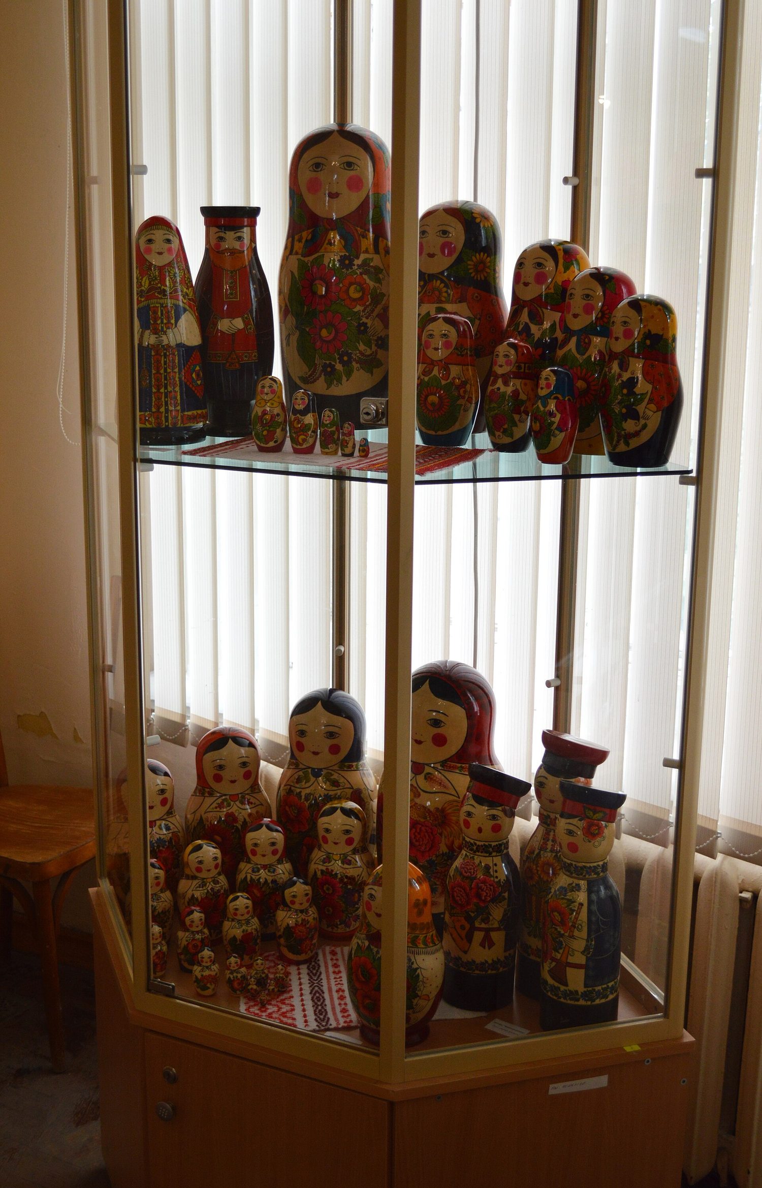
$$h'(x)=5(2x^2+1)^4\cdot\frac{d}{dx}(2x^2+1)=5(2x^2+1)^4\cdot 4x=20x(2x^2+1)^4.$$Matryoshka dolls: the chain rule differentiates nested functions layer by layer — outer first, then the next inside 어휘 연습하기English 한국어 chain rule/tʃeɪn ruːl/ 연쇄 법칙 composite function/ˈkɒmpəzɪt ˈfʌŋkʃn/ 합성 함수 3.2
Implicit Differentiation

Syllabus
지속적 이해 (FUN-3): 미분 규칙을 적용할 수 있는 상황을 파악하면 미분 과정이 단순화됩니다.
학습 목표 FUN-3.D: 암시적으로 정의된 함수의 미분값을 계산한다.
- FUN-3.D.1 연쇄 법칙은 암시적 미분의 기초이다.
출처: College Board AP Course and Exam Description
Some curves are defined implicitly – by an equation in $x$ and $y$ that is not solved for $y$, such as $x^2+y^2=25$. Implicit differentiation 隐函数求导 finds $\dfrac{dy}{dx}$ without solving for $y$ first. It is just the chain rule, treating $y$ as a function of $x$.
The method: differentiate both sides with respect to $x$; every time you differentiate a $y$-term, multiply by $\dfrac{dy}{dx}$ (the chain rule); then solve algebraically for $\dfrac{dy}{dx}$. For $x^2+y^2=25$:
$$2x + 2y\frac{dy}{dx}=0 \;\Longrightarrow\; \frac{dy}{dx} = -\frac{x}{y}.$$Worked example. Find the tangent line to the circle $x^2+y^2=25$ at the point $(3,4)$. From above $\dfrac{dy}{dx}=-\dfrac{x}{y}=-\dfrac{3}{4}$ there, so the tangent is
$$y-4=-\tfrac{3}{4}(x-3).$$Notice the tangent is perpendicular to the radius, as geometry promises – a good sanity check.Implicit differentiation gives the tangent to a circle, perpendicular to the radius Exam skill – "Show that $\dfrac{dy}{dx}=\ldots$". This exact prompt appears most years (e.g. "Show that $\dfrac{dy}{dx}=\dfrac{2y}{y^2-2x}$"). Because the target is given, you must show every algebra step cleanly: differentiate both sides, use the product/chain rules on mixed $xy$ terms, collect all $\dfrac{dy}{dx}$ terms on one side, factor, and divide. A correct final line that skips the algebra earns little. Follow-up parts then ask for a tangent line, or where the tangent is horizontal ($\tfrac{dy}{dx}=0$, so the numerator is $0$) or vertical (the denominator is $0$).
어휘 연습하기English 한국어 Implicit differentiation/ɪmˈplɪsɪt ˌdɪfəˌrenʃɪˈeɪʃn/ 은밀 미분법 3.3
Differentiating Inverse Functions
Syllabus
지속적 이해 (FUN-3): 미분 규칙을 적용할 수 있는 상황을 파악하면 미분 과정이 단순화됩니다.
학습 목표 FUN-3.E: 역함수와 역삼각함수의 미분값을 계산한다.
- FUN-3.E.1 연쇄 법칙과 역함수의 정의를 사용하여 역함수의 미분값을 구할 수 있으며, 이는 미분값이 존재할 때만 가능하다.
출처: College Board AP Course and Exam Description
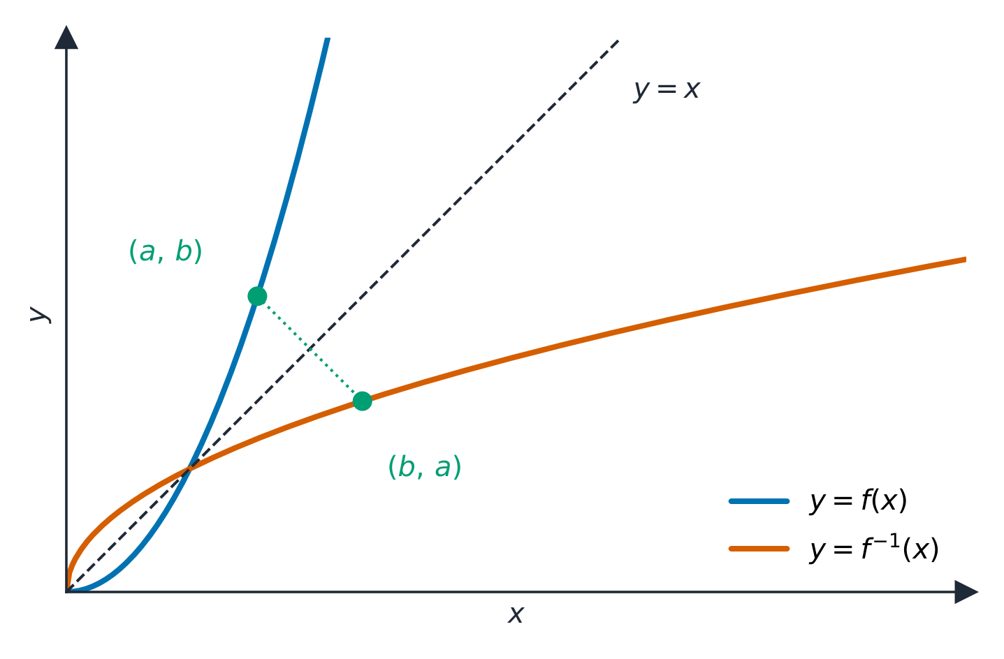
If $g$ is the inverse function 反函数 of $f$ (so $f(g(x))=x$), the chain rule links their derivatives:
$$g'(x) = \frac{1}{f'\big(g(x)\big)},\qquad\text{provided } f'\big(g(x)\big)\neq 0.$$In words: the derivative of the inverse at a point is the reciprocal 倒数 of the derivative of the original function at the matching point. A common exam setup gives a table and a point $(a,b)$ on $f$ (so $(b,a)$ is on $g$), then asks for $g'(b)=\dfrac{1}{f'(a)}$.The inverse function is the mirror image of the function in the line y = x Worked example. Suppose $f(2)=5$ and $f'(2)=3$, and $g$ is the inverse of $f$. Because $(2,5)$ lies on $f$, the point $(5,2)$ lies on $g$, and
$$g'(5)=\frac{1}{f'(2)}=\frac{1}{3}.$$The graphs of $f$ and $g$ are mirror images across $y=x$, so their slopes at matching points are reciprocals.탐색하기지수 함수와 그 역함수인 로그
y = a·e^(bx) + c
역함수는 $y=x$를 기준으로 대칭이며, 기울기는 서로 역수 관계입니다: $\frac{d}{dx}[f^{-1}(x)] = \dfrac{1}{f'(f^{-1}(x))}$. 한쪽이 가파르면 다른 쪽의 역함수는 완만합니다.
어휘 연습하기English 한국어 inverse function/ɪnˈvɜːs ˈfʌŋkʃn/ 역함수 reciprocal/rɪˈsɪprəkl/ 역수 3.4
Differentiating Inverse Trigonometric Functions
Syllabus
지속적 이해 (FUN-3): 미분 규칙을 적용할 수 있는 상황을 파악하면 미분 과정이 단순화됩니다.
학습 목표 FUN-3.E: 역함수와 역삼각함수의 미분값을 계산한다.
- FUN-3.E.2 연쇄 법칙을 역함수의 정의에 적용하거나, 역함수의 미분 공식을 사용하여 역삼각함수의 미분값을 구할 수 있다.
출처: College Board AP Course and Exam Description
The same idea gives the derivatives of the inverse trigonometric functions 反三角函数. The three you should know:
$$\frac{d}{dx}\arcsin x = \frac{1}{\sqrt{1-x^2}}, \quad \frac{d}{dx}\arctan x = \frac{1}{1+x^2}, \quad \frac{d}{dx}\text{arcsec}\,x = \frac{1}{|x|\sqrt{x^2-1}}.$$Combine these with the chain rule when the input is itself a function, e.g. $\dfrac{d}{dx}\arctan(3x)=\dfrac{3}{1+9x^2}$.어휘 연습하기English 한국어 inverse trigonometric functions/ɪnˈvɜːs ˌtrɪɡənəʊˈmetrɪk ˈfʌŋkʃnz/ 역삼각함수 3.5
Selecting Procedures for Calculating Derivatives
Syllabus
이 주제는 적절한 미분 계산 절차를 선택하는 기술에 집중하도록 설계되었다. 학생들은 미분값 계산과 관련된 모든 학습 목표를 언제 및 어떻게 적용할지 연습할 기회가 주어져야 한다.
출처: College Board AP Course and Exam Description
A skill topic: real derivatives mix several rules, so read the structure of the expression first, from the outside in.
- Is it a sum? Differentiate term by term.
- A product or quotient? Apply that rule, and expect to use the chain rule inside.
- A composite (something inside something)? Chain rule.
- Given implicitly? Implicit differentiation.
Name the outermost operation, apply its rule, and recurse inward. Neatness prevents the sign and bookkeeping errors that cost marks.
3.6
Calculating Higher-Order Derivatives
Syllabus
지속적 이해 (FUN-3): 미분 규칙을 적용할 수 있는 상황을 파악하면 미분 과정이 단순화됩니다.
학습 목표 FUN-3.F: 함수의 고계 미분값을 결정한다.
- FUN-3.F.1 $f'$를 미분하면 $f''$인 이계 미분값을 얻으며, 이는 $f'$의 미분값이 존재할 때 가능하고, 이 과정을 반복하면 $f$의 고계 미분값을 얻을 수 있다.
- FUN-3.F.2 고계 미분값은 다양한 표기법으로 표현된다. $y = f(x)$에 대해 이계 미분값의 표기법은 $\dfrac{d^2 y}{dx^2}$, $f''(x)$, $y''$가 포함된다. 고계 미분값은 $\dfrac{d^n y}{dx^n}$ 또는 $f^{(n)}(x)$로 나타낼 수 있다.
출처: College Board AP Course and Exam Description
Differentiating $f'$ produces the second derivative 二阶导数 $f''$; repeating gives higher-order derivatives. The notations:
$$f''(x)=\frac{d^2y}{dx^2}=y'', \qquad\text{and in general}\qquad f^{(n)}(x)=\frac{d^n y}{dx^n}.$$The second derivative measures how the slope is changing; it drives concavity 凹凸性 and acceleration in later units. To find $f''$ implicitly, differentiate the expression for $\dfrac{dy}{dx}$ again (with the quotient and chain rules), then substitute $\dfrac{dy}{dx}$ back in.탐색하기기울기의 기울기: 이계도함수
y = ax³ + bx² + cx + d
다시 미분하면 이계도함수를 얻으며, 이는 기울기가 변하는 속도를 의미합니다. 접선의 기울기 자체가 증가하는 곳에서는 곡선이 위로 볼록(오목)하게 굽습니다.
어휘 연습하기English 한국어 second derivative/ˈsekənd dɪˈrɪvətɪv/ 이계 도함수Unless second derivative. concavity/kənˈkævɪti/ 볼록성 3.6
Exam tips
- Use the chain rule for composite functions — differentiate the outside, then multiply by the derivative of the inside (the most-forgotten factor).
- For implicit differentiation, differentiate both sides with respect to $x$ and attach $\tfrac{dy}{dx}$ each time $y$ is differentiated, then solve.
- Get the second derivative by differentiating twice (velocity → acceleration).
- Combine rules carefully in layered expressions (chain inside product, etc.).
- The inverse function's graph is the reflection in $y=x$; its slope is the reciprocal of the original's at the matching point.
-
4
미분의 맥락적 적용
수업 보기4.1
Interpreting the Derivative in Context
Syllabus
지속적 이해 (CHA-3): 미분은 변화율과 관련된 실제 문제를 해결하게 해준다.
학습 목표 CHA-3.A: 맥락에서 미분의 의미를 해석한다.
- CHA-3.A.1 함수의 미분은 독립변수에 대한 순간 변화율로 해석될 수 있다.
- CHA-3.A.2 미분은 적용 맥락에서 변화율에 관한 정보를 표현하는 데 사용될 수 있다.
- CHA-3.A.3 $f'(x)$의 단위는 $f$의 단위에서 $x$의 단위를 나눈 값이다.
출처: College Board AP Course and Exam Description
Once you can compute derivatives, you use them to describe the real world. The derivative $f'(x)$ is the instantaneous rate of change of $f$ with respect to its input. Reading and reporting this rate correctly is a graded skill.
Units matter. The unit of $f'(x)$ is the unit of $f$ divided by the unit of $x$. If $C(t)$ is a number of acres and $t$ is in weeks, then $C'(t)$ is in acres per week. On the exam, "Using correct units, interpret the meaning of $g'(140)$" wants a full sentence: the value, the quantity, the rate word "per", and the moment. For example: "$g'(140)=2.3$ means that at $x=140$, the quantity is increasing at about $2.3$ units per unit of $x$."
4.2
Straight-Line Motion: Position, Velocity, and Acceleration
Syllabus
지속적 이해 (CHA-3): 미분은 변화율과 관련된 실제 문제를 해결하게 해준다.
학습 목표 CHA-3.B: 적용 맥락에서 변화율을 계산한다.
- CHA-3.B.1 미분은 위치, 속력, 속도, 가속도와 관련된 직선 운동 문제를 해결하는 데 사용될 수 있다.
출처: College Board AP Course and Exam Description
For a particle moving on a line, three functions of time are linked by differentiation:
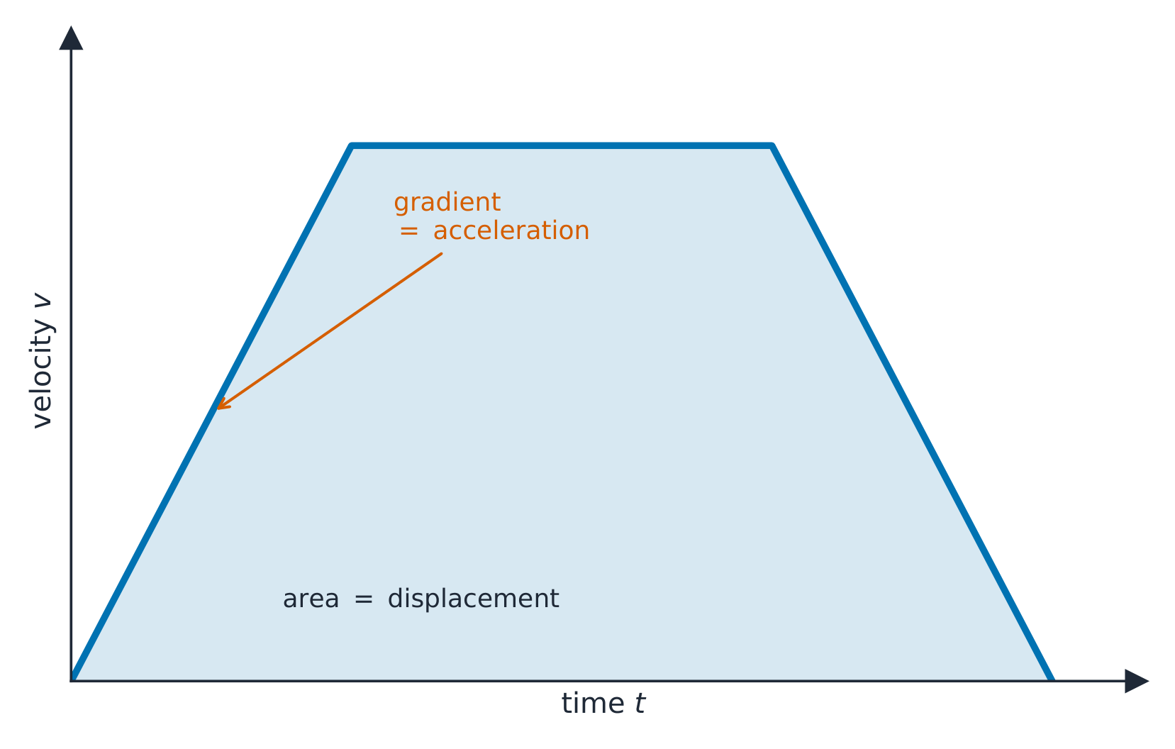
On a velocity-time graph, the area is displacement and the gradient is acceleration - position 位置 $s(t)$;
- velocity 速度 $v(t)=s'(t)$ – signed; its sign gives direction;
- acceleration 加速度 $a(t)=v'(t)=s''(t)$.
Key readings (frequent exam parts):
- The particle is at rest 静止 when $v(t)=0$.
- It moves right/up when $v(t)>0$ and left/down when $v(t)<0$; it changes direction where $v$ changes sign.
- Speed 速率 is $|v(t)|$. Speed is increasing when $v$ and $a$ have the same sign (the particle is speeding up), and decreasing when they have opposite signs.
Worked example. A particle moves with $s(t)=t^3-6t^2+9t$. Then $v(t)=3t^2-12t+9=3(t-1)(t-3)$, so it is at rest at $t=1$ and $t=3$, and changes direction at each. At $t=2$, $v(2)=3(1)(-1)=-3<0$ (moving left) and $a(2)=6(2)-12=0$; just after, $a>0$ while $v<0$, so it is slowing down there. Distinguish carefully between velocity (has direction) and speed (does not) – the exam tests this exact difference.
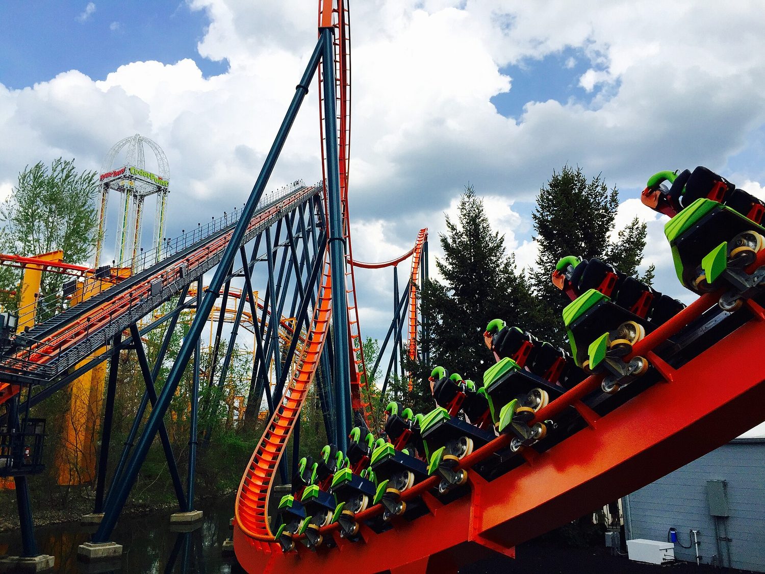
A roller coaster is calculus you can feel: velocity is the derivative of position, and acceleration is the derivative of velocity 탐색하기속도는 위치의 기울기입니다
y = ax³ + bx² + cx + d
직선 운동에서 속도는 위치의 도함수(기울기)이고, 가속도는 속도의 도함수입니다. 점을 밀어서 순간 속도를 확인하세요.
어휘 연습하기English 한국어 position/pəˈzɪʃn/ 위치 velocity/vəˈlɒsɪti/ 속도 acceleration/əkˌseləˈreɪʃn/ 가속도 at rest/æt rest/ 정지 상태임 Speed/spiːd/ 속도 4.3
Rates of Change Beyond Motion
Syllabus
지속적 이해 (CHA-3): 미분은 변화율과 관련된 실제 문제를 해결하게 해준다.
학습 목표 CHA-3.C: 적용 맥락에서 변화율을 해석한다.
- CHA-3.C.1 미분은 적용 맥락에서의 변화율 문제를 해결하는 데 사용될 수 있다.
출처: College Board AP Course and Exam Description
The same derivative idea models any changing quantity: a draining tank, a spreading population, a cooling cup. Whenever a problem says "the rate at which...", it is describing a derivative. Read the units to know which quantity's rate you have, then interpret in context.
4.4
Introduction to Related Rates
Syllabus
지속적 이해 (CHA-3): 미분은 변화율과 관련된 실제 문제를 해결하게 해준다.
학습 목표 CHA-3.D: 적용 맥락에서 종속 변수의 변화율을 계산한다.
- CHA-3.D.1 연쇄 법칙은 종속 변수의 변화율 문제에서 변수를 동일한 독립변수에 대해 미분하는 기초이다.
- CHA-3.D.2 곱의 미분법이나商的 미분법과 같은 다른 미분 규칙도 동일한 독립변수에 대해 모든 변수를 미분하는 데 필요할 수 있다.
출처: College Board AP Course and Exam Description
Related rates: a sliding ladder In a related rates 相关变化率 problem, several quantities change together over time, and you know some rates but want another. The engine is the chain rule: differentiate a relationship with respect to time $t$. Every variable becomes a function of $t$, so each derivative picks up a "$\,/\,dt$" factor. Product and quotient rules may also be needed.
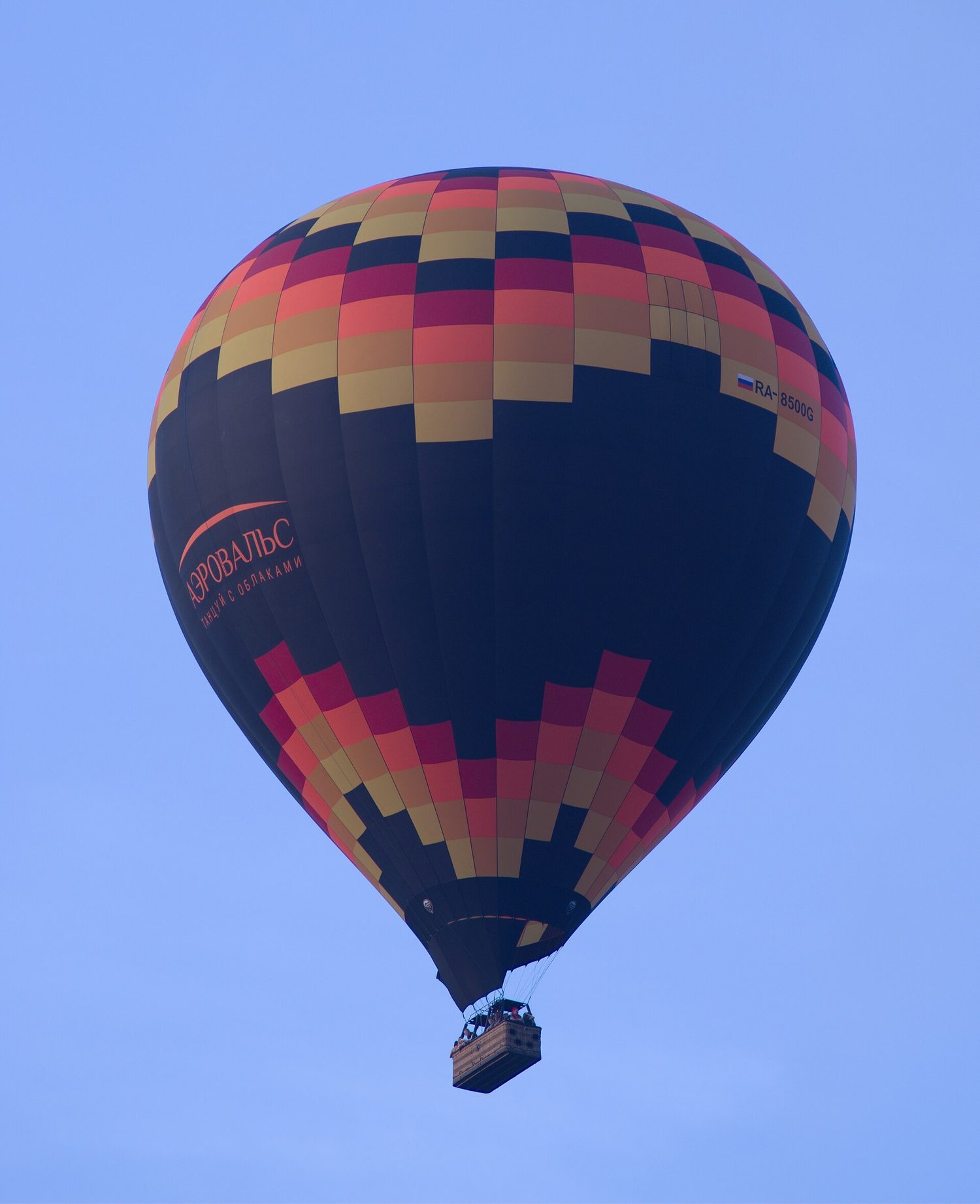
A rising balloon: related rates link how fast radius, volume and height change together 어휘 연습하기English 한국어 related rates/rɪˈleɪtɪd reɪts/ 연관 변수율 4.5
Solving Related Rates Problems
Syllabus
지속적 이해 (CHA-3): 미분은 변화율과 관련된 실제 문제를 해결하게 해준다.
학습 목표 CHA-3.E: 적용 맥락에서 종속 변수의 변화율을 해석한다.
- CHA-3.E.1 미분은 종속 변수의 변화율 문제를 해결하는 데 사용될 수 있다; 즉, 한 양의 변화율을 알고 있는 다른 양들과 연관시켜 그 양의 변화율을 찾는 것이다.
출처: College Board AP Course and Exam Description
A reliable procedure – and a full-credit template on the exam:
- Name the variables and write down the given rates and the unknown rate (e.g. "$\dfrac{dh}{dt}=-2$ cm/day, find $\dfrac{dV}{dt}$").
- Write an equation relating the quantities (often a geometric or volume formula).
- Differentiate both sides with respect to $t$ (chain rule) – before substituting numbers.
- Substitute the known values at the instant of interest, and solve for the unknown rate.
- State the answer with units and the correct sign (a decreasing quantity has a negative rate).
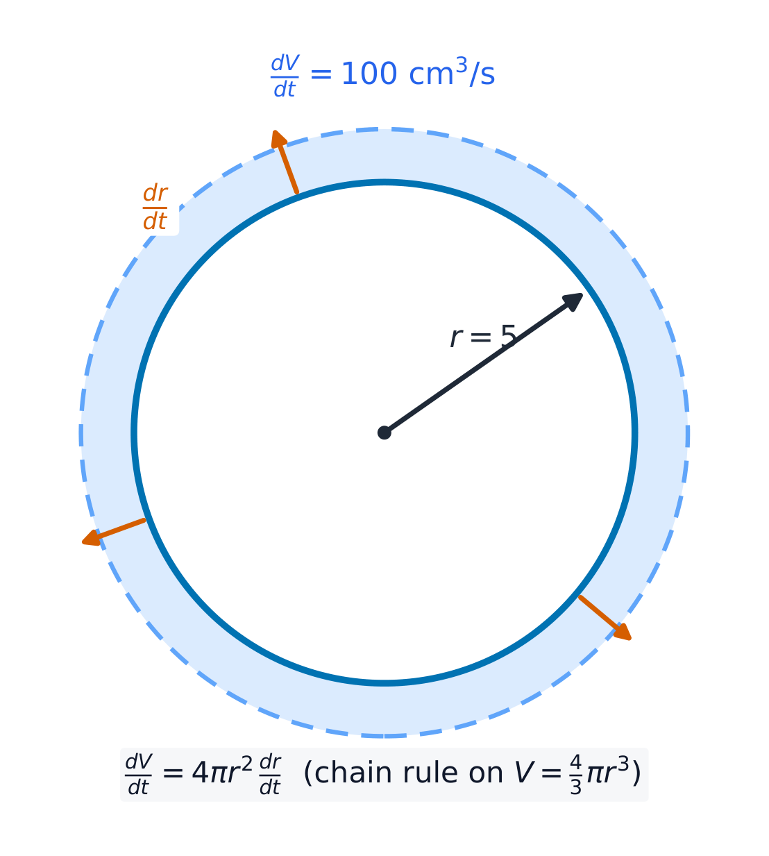
Worked example. Air is pumped into a spherical balloon so its volume grows at $\dfrac{dV}{dt}=100\ \text{cm}^3/\text{s}$. How fast is the radius growing when $r=5\ \text{cm}$? Start from $V=\tfrac43\pi r^3$ and differentiate with respect to $t$ first:
$$\frac{dV}{dt}=4\pi r^2\frac{dr}{dt}\;\Rightarrow\;100=4\pi(5)^2\frac{dr}{dt}\;\Rightarrow\;\frac{dr}{dt}=\frac{100}{100\pi}=\frac{1}{\pi}\approx 0.32\ \text{cm/s}.$$Substituting $r=5$ too early is the classic error – differentiate the general relationship, then plug in.An inflating balloon links dV/dt and dr/dt through the chain rule 4.6
Local Linearity and Linearization
Syllabus
지속적 이해 (CHA-3): 미분은 변화율과 관련된 실제 문제를 해결하게 해준다.
학습 목표 CHA-3.F: 접선의 방정식을 사용하여 곡선 위의 값을 근사한다.
- CHA-3.F.1 접선은 접점 근처에서 함수의 국소 선형 근사의 그래프이다.
- CHA-3.F.2 접선 근사 approximation에서, 접점 근처에서의 함수의 거동은 해당 접선 값이 대응하는 함수 값에 대한 과소평가인지 과대평가인지를 결정할 수 있습니다.
출처: College Board AP Course and Exam Description
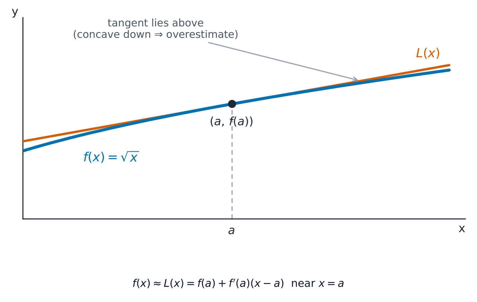
Local linearity and linearisation Near a point of tangency, a smooth curve looks like its tangent line – this is local linearity 局部线性. So the tangent line gives a linear approximation 线性近似 (linearization) of the function near that point:
$$f(x) \approx L(x) = f(a) + f'(a)(x-a).$$Use it to estimate $f$ at an $x$ close to $a$.The tangent line is the best linear approximation to the curve near the point of tangency Worked example. Estimate $\sqrt{4.1}$. Take $f(x)=\sqrt{x}$ and $a=4$: $f(4)=2$ and $f'(x)=\dfrac{1}{2\sqrt{x}}$ so $f'(4)=\dfrac14$. Then $L(4.1)=2+\tfrac14(4.1-4)=2.025$ (the true value is $2.0248\ldots$). Because $\sqrt{x}$ is concave down, the tangent lies above the curve, so this is a slight overestimate 高估 – justify over/under with the sign of $f''$.
탐색하기접선을 이용해 곡선 근사하기
y = ax³ + bx² + cx + d
국소 선형성: 점 근처에서 매끄러운 곡선은 접선과 비슷해 보이므로, 접선은 주변 값들의 좋은 선형 근사를 제공합니다.
어휘 연습하기English 한국어 local linearity/ˈləʊkl lɪˈnɪərɪti/ 국소 선형성 linear approximation/ˈlɪnɪə əˌprɒksɪˈmeɪʃn/ 선형 근사 overestimate/ˌəʊvəˈrestɪmət/ 과대평가(overestimate) 4.7
L'Hospital's Rule for Indeterminate Forms
Syllabus
지속적 이해 (LIM-4): 로피탈의 법칙은 특정 불정형의 극한을 구하는 데 도움을 줍니다.
학습 목표 LIM-4.A: 불정형을 나타내는 함수의 극한을 구합니다.
- LIM-4.A.1 두 함수의 비가 극한에서 $\dfrac{0}{0}$ 또는 $\dfrac{\infty}{\infty}$로趋向할 때, 이러한 형태는 불정형이라고 합니다.
- 배제 문구: $\infty - \infty$와 같이 무정형 형태(indeterminate forms)는还有许多其他的,例如,但这些内容不会在AP微积分AB或BC考试中评估。然而,如果时间允许,教师可以包含这些主题。
- LIM-4.A.2 불정형 $\dfrac{0}{0}$ 또는 $\dfrac{\infty}{\infty}$의 극한은 로피탈 규칙을 사용하여 계산할 수 있습니다.
출처: College Board AP Course and Exam Description
When direct substitution in a quotient of limits gives the indeterminate form 未定式 $\dfrac{0}{0}$ or $\dfrac{\infty}{\infty}$, you may use L'Hospital's Rule 洛必达法则:
$$\lim_{x\to c}\frac{f(x)}{g(x)} = \lim_{x\to c}\frac{f'(x)}{g'(x)},$$provided the right-hand limit exists. Differentiate the top and bottom separately (this is not the quotient rule), then try the limit again. First confirm the form really is $\tfrac{0}{0}$ or $\tfrac{\infty}{\infty}$ – applying the rule to any other form is a mistake.Worked example. Evaluate $\displaystyle\lim_{x\to 0}\frac{\sin x}{x}$. Substituting gives $\tfrac00$, so differentiate top and bottom: $\displaystyle\lim_{x\to 0}\frac{\cos x}{1}=\cos 0=1$ – confirming the famous limit from Unit 1.
어휘 연습하기English 한국어 indeterminate form/ˌɪndɪˈtɜːmɪnət fɔːm/ 부정정 형식 L'Hospital's Rule/ˈelhɒspɪtlz ruːl/ L'Hospital 법칙 4.7
Exam tips
- In motion problems: velocity is the derivative of position, acceleration the derivative of velocity; speed increases when velocity and acceleration share a sign.
- For related rates, differentiate the relating equation with respect to time, then substitute the given values last.
- Use the tangent line for a linear approximation near a known point; it is accurate only close by.
- Read the sign of a rate: positive means the quantities move together, negative means opposite.
- Always state units and interpret the answer in context.
-
5
미분의 분석적 적용
수업 보기5.1
The Mean Value Theorem
Syllabus
지속적 이해(FUN-1): 존재 정리는 특정 구간에서 함수의 행동을 정확히 locating하지 않고도 결론을 내릴 수 있게 해줍니다.
학습 목표 FUN-1.B: 평균값 정리를 구간에서 적용하여 함수에 대한 결론을 정당화합니다.
- FUN-1.B.1 함수 $f$가 구간 $[a, b]$에서 연속이고 구간 $(a, b)$에서 가미 가능하면, 평균값 정리에 의해 이 개구간 내에 순간 변화율이 구간 전체의 평균 변화율과 같아지는 점이 존재함을 보장합니다.
출처: College Board AP Course and Exam Description
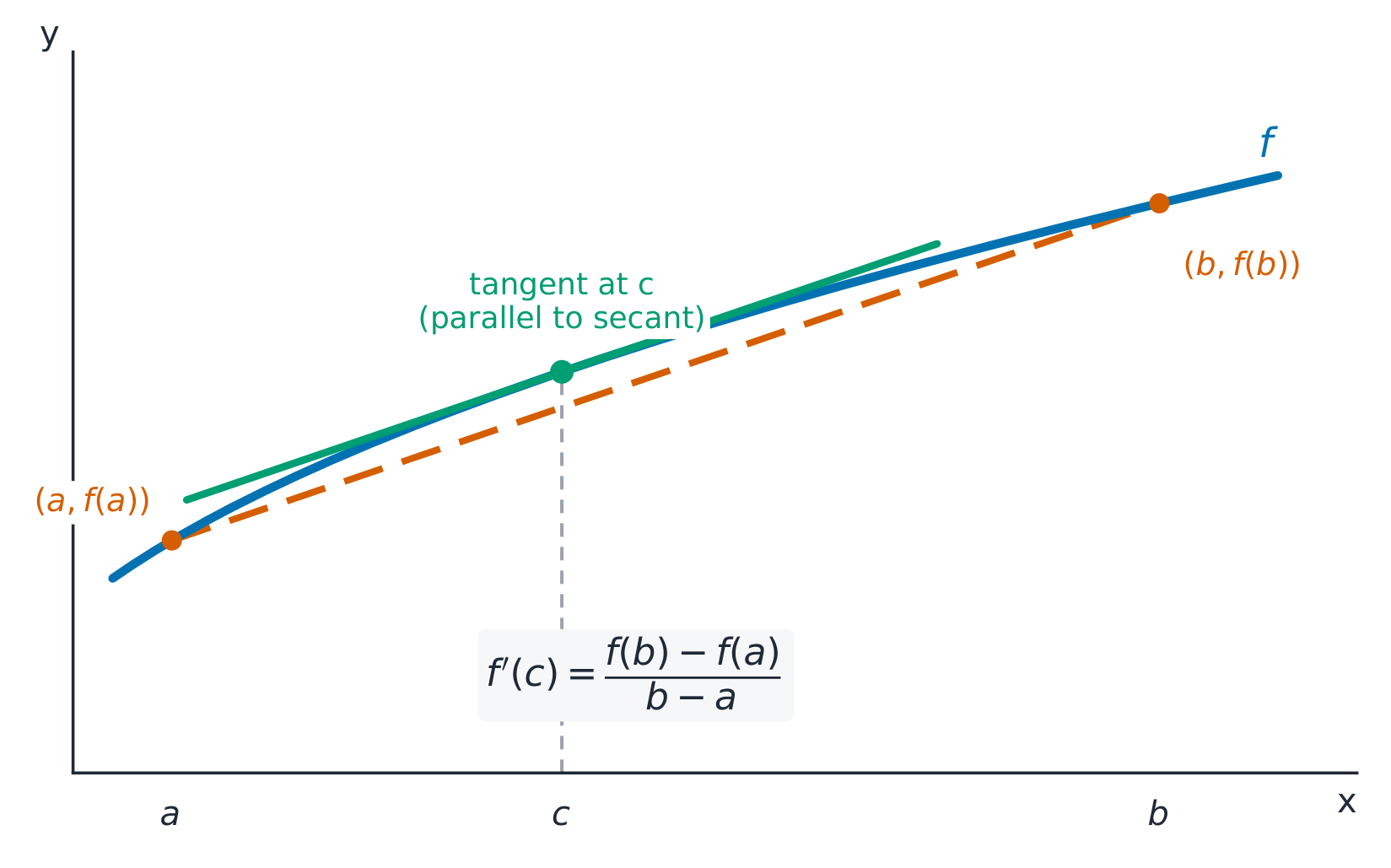
The Mean Value Theorem The Mean Value Theorem 中值定理 (MVT) links the average rate of change to an instantaneous one:
If $f$ is continuous on $[a,b]$ and differentiable on $(a,b)$, then there is at least one point $c$ in $(a,b)$ where
$$f'(c) = \frac{f(b)-f(a)}{b-a}.$$In words: somewhere inside the interval, the instantaneous rate equals the average rate. Geometrically, some tangent line is parallel to the line joining the endpoints.
The Mean Value Theorem: some tangent is parallel to the secant over the interval Exam skill. Like the IVT, the MVT is an existence theorem, and questions ask you to justify. Full credit needs: (1) state $f$ is continuous on $[a,b]$ and differentiable on $(a,b)$; (2) compute the average rate $\frac{f(b)-f(a)}{b-a}$; (3) conclude "by the MVT there is a $c$ in $(a,b)$ with $f'(c)$ equal to that value." Both hypotheses must be named.
Worked example. Verify the MVT for $f(x)=x^2$ on $[1,3]$. It is a polynomial, so continuous and differentiable everywhere. The average rate is $\dfrac{f(3)-f(1)}{3-1}=\dfrac{9-1}{2}=4$. Setting $f'(c)=2c=4$ gives $c=2$, which does lie in $(1,3)$ – the guaranteed point.
탐색하기평균값 정리
y = ax³ + bx² + cx + d
MVT는 접선이 할선과 평행한 점이 존재함을 보장합니다 — 구간 내부의某 지점에서 순간 변화율이 평균 변화율과 같습니다.
어휘 연습하기English 한국어 Mean Value Theorem/miːn ˈvæljuː ˈθɪərəm/ 평균값 정리 5.2
Extreme Values and Critical Points
Syllabus
지속적 이해(FUN-1): 존재 정리는 특정 구간에서 함수의 행동을 정확히 locating하지 않고도 결론을 내릴 수 있게 해줍니다.
학습 목표 FUN-1.C: 극대값 정리를 적용하여 함수에 대한 결론을 정당화합니다.
- FUN-1.C.1 함수 $f$가 구간 $(a, b)$에서 연속이면, 극한값 정리에 의해 $f$는 구간 $[a, b]$에서 최소값과 최대값이 각각 적어도 하나씩 존재함을 보장합니다.
- FUN-1.C.2 함수 위에서 첫 번째 도함수가 0이거나 존재하지 않는 점은 해당 함수의 임계점입니다.
- FUN-1.C.3 모든 국소(상대) 극값은 함수의 임계점에서 발생하지만, 모든 임계점이 국소 극값인 것은 아닙니다.
출처: College Board AP Course and Exam Description
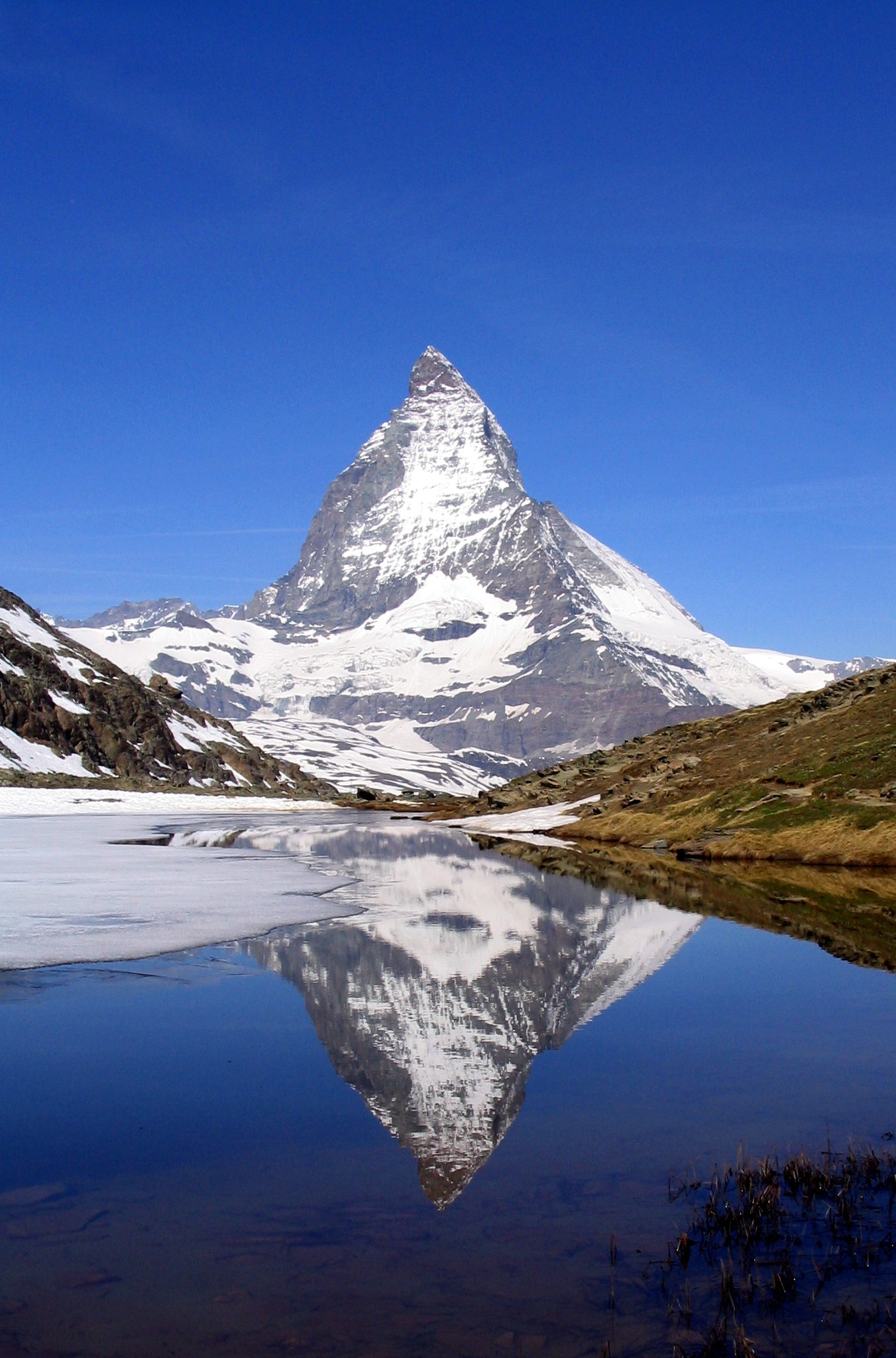
A mountain peak reflected in a lake: extrema and critical points mark highest and lowest values The Extreme Value Theorem 极值定理 (EVT) guarantees extremes exist: a function continuous on a closed interval $[a,b]$ attains both an absolute maximum and an absolute minimum on it.
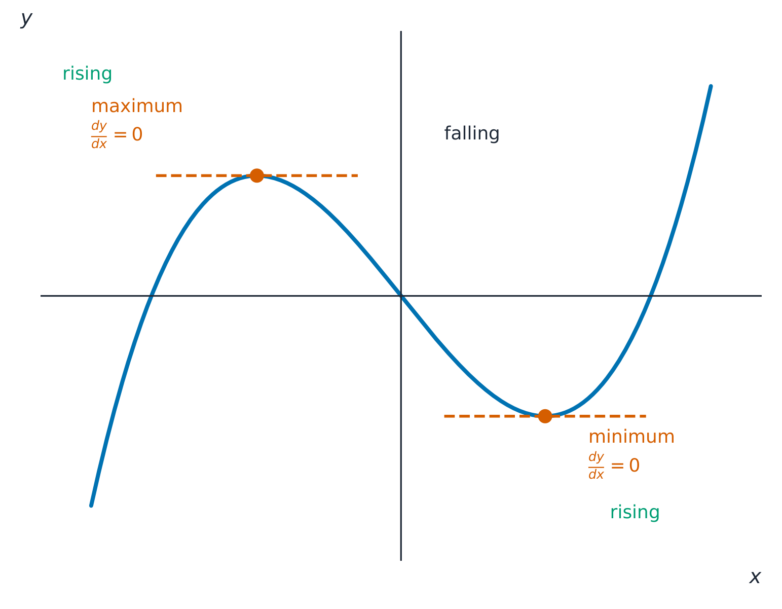
At a maximum or minimum the derivative is zero A critical point 临界点 is an interior point where $f'(x)=0$ or $f'(x)$ does not exist. All local (relative) extrema 局部极值 occur at critical points – but not every critical point is an extremum. So critical points are the candidates; you must test each.
어휘 연습하기English 한국어 Extreme Value Theorem/ekˈstriːm ˈvæljuː ˈθɪərəm/ 극한값 정리 critical point/ˈkrɪtɪkl pɔɪnt/ 임계점 local (relative) extrema/ˈləʊkl ekˈstremə/ 국소(상대) 극값 5.3
Increasing and Decreasing Intervals
Syllabus
지속적 이해 (FUN-4): 함수의 도함수를 통해 함수의 일부 거동을 이해할 수 있습니다.
학습 목표 FUN-4.A: 도함수의 거동에 기반하여 함수의 거동에 대한 결론을 정당화합니다.
- FUN-4.A.1 함수의 첫 번째 도함수는 함수와 그 그래프에 대한 정보를 제공하며,其中包括函数增加或减少的区间。
출처: College Board AP Course and Exam Description
The first derivative tells you where $f$ rises or falls:
- $f'(x) > 0$ on an interval $\Rightarrow$ $f$ is increasing 递增 there;
- $f'(x) < 0$ $\Rightarrow$ $f$ is decreasing 递减.
On the exam, "find the intervals where $f$ is increasing" means: find the critical points, then test the sign of $f'$ between them, and justify with the sign of $f'$ (a stated reason, not just an interval).
어휘 연습하기English 한국어 increasing/ɪnˈkriːsɪŋ/ 증가함 decreasing/ˈdiːkriːsɪŋ/ 감소함 5.4
The First Derivative Test
Syllabus
지속적 이해 (FUN-4): 함수의 도함수를 통해 함수의 일부 거동을 이해할 수 있습니다.
학습 목표 FUN-4.A: 도함수의 거동에 기반하여 함수의 거동에 대한 결론을 정당화합니다.
- FUN-4.A.2 함수의 첫 번째 도함수는 함수의 국소(상대) 극값 위치를 결정할 수 있습니다.
출처: College Board AP Course and Exam Description
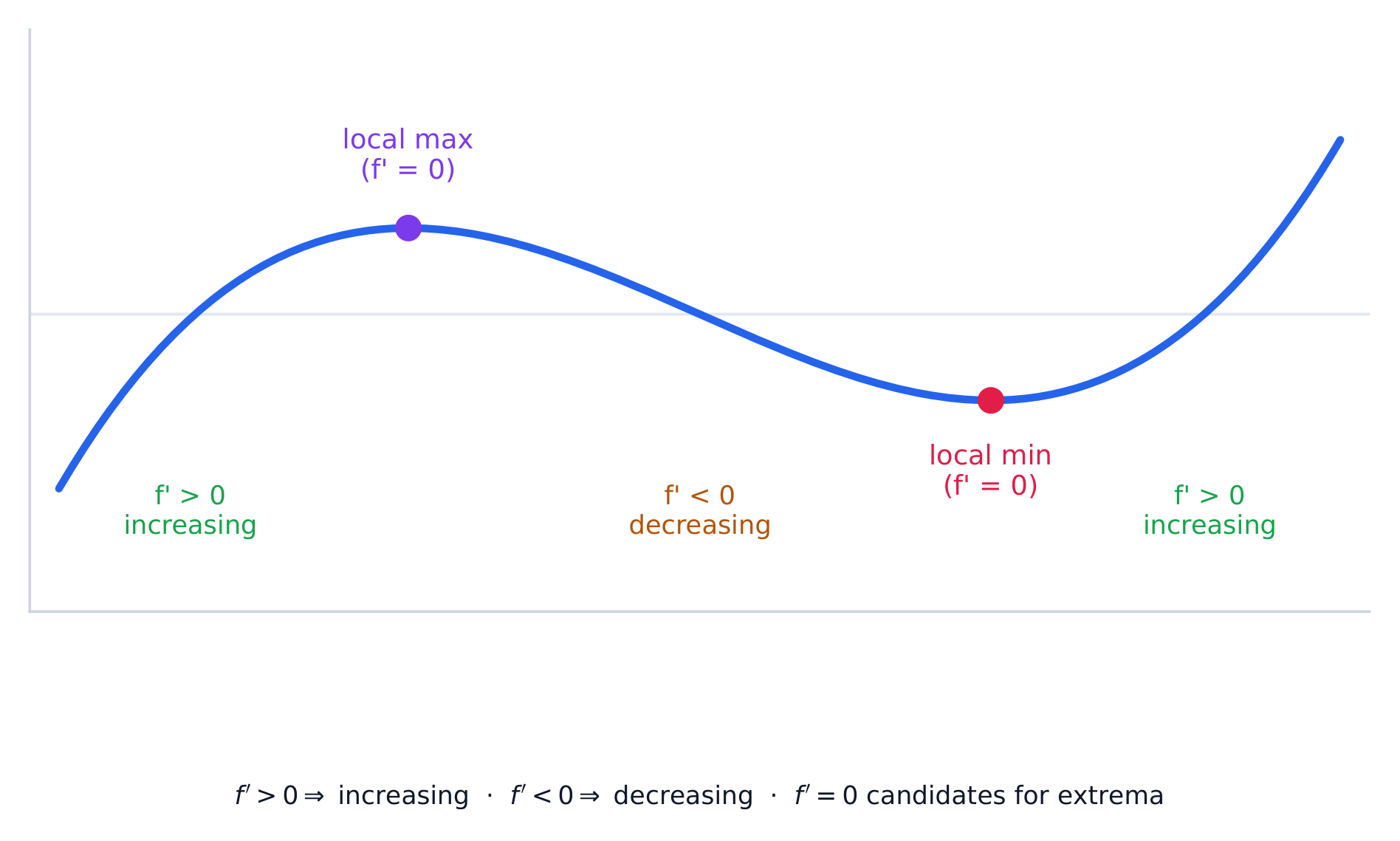
To classify a critical point $x=c$ as a local max, local min, or neither, check how $f'$ changes sign there:
- $f'$ changes $+$ to $-$ at $c$ $\Rightarrow$ local maximum 极大值;
- $f'$ changes $-$ to $+$ at $c$ $\Rightarrow$ local minimum 极小值;
- $f'$ does not change sign $\Rightarrow$ neither.
Always state the sign change as your justification.
Worked example. Classify the critical points of $f(x)=x^3-3x^2$. Here $f'(x)=3x^2-6x=3x(x-2)$, zero at $x=0$ and $x=2$. Testing signs: $f'>0$ for $x<0$, $f'<0$ on $(0,2)$, and $f'>0$ for $x>2$. So $f'$ turns $+\to-$ at $x=0$ (a local maximum, $f(0)=0$) and $-\to+$ at $x=2$ (a local minimum, $f(2)=-4$).
Where $f' > 0$ the graph rises and where $f' < 0$ it falls; a local max sits where $f'$ turns $+$ to $-$, a local min where it turns $-$ to $+$. 어휘 연습하기English 한국어 local maximum/ˈləʊkl ˈmæksɪməm/ 국소 최대점 local minimum/ˈləʊkl ˈmɪnɪməm/ 국소 최소점 5.5
The Candidates Test for Absolute Extrema
Syllabus
지속적 이해 (FUN-4): 함수의 도함수를 통해 함수의 일부 거동을 이해할 수 있습니다.
학습 목표 FUN-4.A: 도함수의 거동에 기반하여 함수의 거동에 대한 결론을 정당화합니다.
- FUN-4.A.3 닫힌 구간에서 함수의 전역(전체) 극값은 오직 임계점이나 경계점에서만 발생할 수 있습니다.
출처: College Board AP Course and Exam Description
On a closed interval, absolute (global) extrema occur only at critical points or endpoints. The candidates test:
- List all critical points in $[a,b]$ and the two endpoints.
- Evaluate $f$ at each candidate.
- The largest output is the absolute maximum; the smallest is the absolute minimum.
Show the table of values – the comparison is the argument.
5.6
Concavity and Points of Inflection
Syllabus
지속적 이해 (FUN-4): 함수의 도함수를 통해 함수의 일부 거동을 이해할 수 있습니다.
학습 목표 FUN-4.A: 도함수의 거동에 기반하여 함수의 거동에 대한 결론을 정당화합니다.
- FUN-4.A.4 함수의 도함수가某开区间上递增(递减)时,该函数的图像在该开区间上是凹向上(下)。
- FUN-4.A.5 함수의 이阶导数 provides information about the function and its graph, including intervals of upward or downward concavity.
- FUN-4.A.6 함수의 이阶导数는 원본 함수의 그래프에서 변곡점을 locating하는 데 사용될 수 있습니다.
출처: College Board AP Course and Exam Description
The second derivative describes bending:
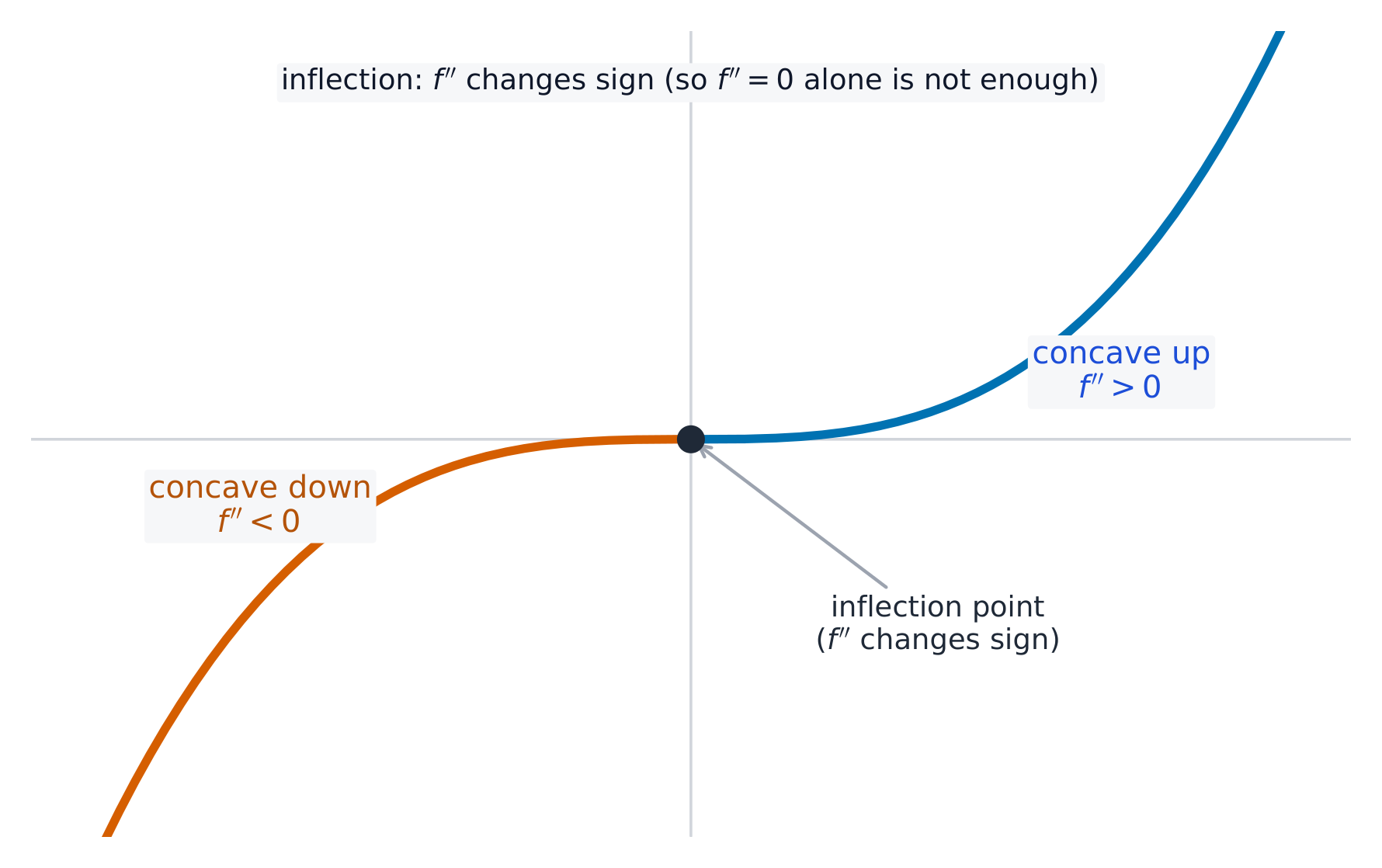
- $f'' > 0$ $\Rightarrow$ $f$ is concave up 上凹 (curving like a cup; $f'$ is increasing);
- $f'' < 0$ $\Rightarrow$ $f$ is concave down 下凹 ($f'$ is decreasing).
A point of inflection 拐点 is where concavity changes, i.e. where $f''$ changes sign (not merely where $f''=0$). Report its $x$-coordinate and justify with the sign change of $f''$.
Concavity comes from the sign of the second derivative; it flips at an inflection point 탐색하기오목성이 바뀌는 지점
y = ax³ + bx² + cx + d
오목성은 $f''$의 부호입니다: 위쪽 오목(오목)은 물을 담을 수 있고, 아래쪽 오목(볼록)은 물을 흘립니다. 변곡점은 오목성이 바뀌는 곳입니다.
어휘 연습하기English 한국어 concave up/kɒnˈkeɪv ʌp/ 오목 위(upward concave) concave down/kɒnˈkeɪv daʊn/ 오목 아래 point of inflection/pɔɪnt ɒv ɪnˈflekʃn/ 변곡점 5.7
The Second Derivative Test
Syllabus
지속적 이해 (FUN-4): 함수의 도함수를 통해 함수의 일부 거동을 이해할 수 있습니다.
학습 목표 FUN-4.A: 도함수의 거동에 기반하여 함수의 거동에 대한 결론을 정당화합니다.
- FUN-4.A.7 함수의 이阶导数는 임계점이 국소(상대) 극대값 또는 극소값의 위치인지 여부를 결정할 수 있습니다.
- FUN-4.A.8 연속 함수가 정의역의 한 구간에서 오직 하나의 임계점만 가지고 있으며, 해당 임계점이 구간에 대한 함수의 상대적(국소) 극값에 대응한다면, 그 임계점은 또한 구간에 대한 함수의 절대적(전체) 극값에도 대응합니다.
출처: College Board AP Course and Exam Description
An alternative way to classify a critical point $c$ where $f'(c)=0$:
- $f''(c) > 0$ $\Rightarrow$ concave up $\Rightarrow$ local minimum;
- $f''(c) < 0$ $\Rightarrow$ concave down $\Rightarrow$ local maximum;
- $f''(c) = 0$ $\Rightarrow$ the test is inconclusive – fall back on the first derivative test.
Special case: if a continuous function has only one critical point on an interval and it is a local extremum, that point is also the absolute extremum there.
5.8
Sketching a Function and Its Derivatives
Syllabus
지속적 이해 (FUN-4): 함수의 도함수를 통해 함수의 일부 거동을 이해할 수 있습니다.
학습 목표 FUN-4.A: 도함수의 거동에 기반하여 함수의 거동에 대한 결론을 정당화합니다.
- FUN-4.A.9 함수와 도함수의 핵심 특징을 식별하고 이를 기하학적, 수치적, 분석적 표현과 연결할 수 있습니다.
- FUN-4.A.10 $f'$와 $f''$로부터 얻은 그래프적, 수치적, 분석적 정보를 활용하여 $f$의 거동을 예측하고 설명할 수 있습니다.
출처: College Board AP Course and Exam Description
Key features of $f$, $f'$, and $f''$ mirror each other. To sketch or read graphs:
- $f$ increasing $\Leftrightarrow$ $f'$ above the axis; $f$ has a local max $\Leftrightarrow$ $f'$ crosses from $+$ to $-$.
- $f$ concave up $\Leftrightarrow$ $f'$ increasing $\Leftrightarrow$ $f''$ above the axis; $f$ has an inflection point $\Leftrightarrow$ $f'$ has a local extremum $\Leftrightarrow$ $f''$ crosses zero.
5.9
Connecting f, f-prime, and f-double-prime
Syllabus
Enduring Understanding Learning Objective Essential Knowledge FUN-4
A function's derivative can be used to understand some behaviors of the function.FUN-4.A
Justify conclusions about the behavior of a function based on the behavior of its derivatives.- FUN-4.A.11 Key features of the graphs of $f$, $f'$, and $f''$ are related to one another.
출처: College Board AP Course and Exam Description
This is the skill of reading one graph to describe another. A very common exam setup gives the graph of $f'$ and asks about $f$: where is $f$ increasing (where $f'>0$), where are $f$'s extrema (where $f'$ crosses zero, with a sign change), where is $f$ concave up (where $f'$ is increasing). Answer questions about $f$ using the height and slope of the $f'$ graph.
탐색하기그래프에서의 기울기와 굽힘
y = ax³ + bx² + cx + d
$f'>0$일 때 함수는 증가하고, $f''>0$일 때 위로 볼록합니다. 접선을 이동하여 $f$의 모양과 도함수의 부호를 연결해 보세요.
5.10
Introduction to Optimization
Syllabus
지속적 이해 (FUN-4): 함수의 도함수를 통해 함수의 일부 거동을 이해할 수 있습니다.
학습 목표 FUN-4.B: 응용 맥락이나 함수 분석에서 최소값 및 최대값을 계산합니다.
- FUN-4.B.1 도함수는 최적화 문제를 해결하는 데 사용될 수 있으며, 이는 주어진 구간에서 함수의 최소값 또는 최대값을 찾는 것입니다.
출처: College Board AP Course and Exam Description
Optimisation: the best box Optimization 最优化 uses the derivative to find the largest or smallest value of a quantity on an interval. It is the candidates/derivative-test machinery applied to a real goal.
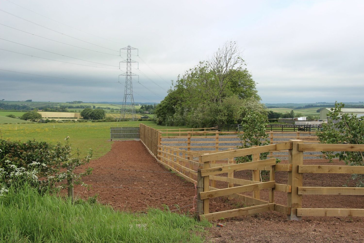
Fenced enclosures: optimization finds the dimensions that maximise area for a fixed fence length 어휘 연습하기English 한국어 Optimization/ˌɒptɪmaɪˈzeɪʃn/ 최적화 5.11
Solving Optimization Problems
Syllabus
지속적 이해 (FUN-4): 함수의 도함수를 통해 함수의 일부 거동을 이해할 수 있습니다.
학습 목표 FUN-4.C: 응용 맥락에서 계산된 최소값 및 최대값을 해석합니다.
- FUN-4.C.1 함수의 최소값 및 최대값은 응용 맥락에서 구체적인 의미를 가집니다.
출처: College Board AP Course and Exam Description
A dependable procedure:
- Write the quantity to optimize as a function of one variable (use a constraint equation to eliminate extras).
- State the interval of allowed inputs.
- Find critical points ($f'=0$ or undefined) and test them (first- or second-derivative test, or candidates test if the interval is closed).
- Answer the question asked, with units and interpretation in context – the maximum area, the minimum cost, etc.
Worked example. A farmer has $100\ \text{m}$ of fence for a rectangular pen against a wall, so only three sides need fencing. Maximize the area. Let the two ends be $x$ and the side parallel to the wall be $y$; the constraint is $2x+y=100$, so $y=100-2x$. The area is
$$A(x)=x(100-2x)=100x-2x^2,\qquad A'(x)=100-4x=0\;\Rightarrow\;x=25.$$Since $A''=-4<0$ this is a maximum, giving $y=50$ and $A=25\times50=1250\ \text{m}^2$.5.12
Behaviors of Implicit Relations
Syllabus
Enduring Understanding Learning Objective Essential Knowledge FUN-4
A function's derivative can be used to understand some behaviors of the function.FUN-4.D
Determine critical points of implicit relations.- FUN-4.D.1 A point on an implicit relation where the first derivative equals zero or does not exist is a critical point of the function.
FUN-4.E
Justify conclusions about the behavior of an implicitly defined function based on evidence from its derivatives.- FUN-4.E.1 Applications of derivatives can be extended to implicitly defined functions.
- FUN-4.E.2 Second derivatives involving implicit differentiation may be relations of $x$, $y$, and $\dfrac{dy}{dx}$.
출처: College Board AP Course and Exam Description
All of this extends to implicitly defined relations. A critical point of an implicit relation is where $\dfrac{dy}{dx}=0$ (horizontal tangent) or is undefined (vertical tangent). Because $\dfrac{dy}{dx}$ is usually a relation in $x$ and $y$, and the second derivative involves $x$, $y$, and $\dfrac{dy}{dx}$, substitute your first-derivative expression back in when finding $\dfrac{d^2y}{dx^2}$, then reason about concavity from its sign.
5.12
Exam tips
- $f'>0$ means increasing, $f'<0$ decreasing; candidates for extrema are where $f'=0$ or is undefined.
- Classify a critical point with the first-derivative sign change or the second-derivative test ($f''>0$ minimum, $f''<0$ maximum).
- $f''>0$ is concave up, $f''<0$ concave down; a point of inflection is where concavity changes ($f''$ changes sign).
- For an absolute extremum on a closed interval, also check the endpoints.
- Justify every conclusion by citing the sign of $f'$ or $f''$ — the exam demands the reasoning, not just the answer.
-
6
적분과 변화의 축적
수업 보기6.1
Exploring Accumulations of Change
Syllabus
지속적 이해 (CHA-4): 정적분은 구간 내에서의 변화량 축적 문제를 해결할 수 있게 해준다.
학습 목표 CHA-4.A: 변화율 그래프와 관련된 면적의 의미를 맥락 속에서 해석한다.
- CHA-4.A.1 변화율 함수의 그래프와 $x$축 사이의 영역의 면적은 변화량의 축적을 나타낸다.
- CHA-4.A.2 일부 경우, 변화량 축적은 기하학적 방법을 통해 계산할 수 있다.
- CHA-4.A.3 어떤 구간에서 변화양이 양수(음수)이면, 축적된 변화량 역시 양수(음수)이다.
- CHA-4.A.4 변화율로 정의된 영역의 면적의 단위는 변화율의 단위와 독립 변수의 단위를 곱한 값이다.
출처: College Board AP Course and Exam Description
A water tank: integration accumulates change — total volume from a rate of flow Differentiation found rates. Integration runs the idea in reverse: given a rate of change, it finds the accumulated change 累积变化. The key picture: the area between the graph of a rate function and the $x$-axis gives the total accumulation.
- If the rate is positive over an interval, the accumulated change is positive; if negative, negative. Area below the axis counts as negative.
- Simple regions (triangles, rectangles) can be found with geometry 几何.
- Units: the area's unit is the rate's unit times the input's unit. A rate in vehicles-per-hour times hours gives vehicles.
어휘 연습하기English 한국어 accumulated change/əˈkjuːmjʊleɪtɪd tʃeɪndʒ/ 누적 변화량 geometry/dʒiˈɒmətri/ 기하학 6.2
Approximating Areas with Riemann Sums

Syllabus
지속적 이해 (LIM-5): 정적분은 기하학적 및 수치적 방법을 사용하여 근사할 수 있다.
학습 목표 LIM-5.A: 기하학적 및 수치적 방법을 사용하여 정적분을 근사한다.
- LIM-5.A.1 정적분은 그래프, 수치, 분석적, 언어적으로 표현된 함수에 대해 근사할 수 있다.
- LIM-5.A.2 정적분은 좌측 리만 합, 우측 리만 합, 중점 리만 합 또는 사다리꼴 합을 사용하여 근사할 수 있으며, 근사는 균등 분할或非等分을 사용하여 계산할 수 있다.
- LIM-5.A.3 정적분은 수치적 방법을 사용하여 근사할 수 있으며, 이 과정에서 기술적 도구(Technology)를 사용하거나 사용하지 않을 수 있다.
- LIM-5.A.4 함수의 성질에 따라 정적분의 근사값이 실제 정적분 값에 비해 과소평가(underestimate)인지 과대평가(overestimate)인지를 판단할 수 있다.
출처: College Board AP Course and Exam Description
The integral as area (Riemann sums) Trapezoidal sums approximate area When exact area is hard, approximate it with a Riemann sum 黎曼和 – split the interval into subintervals and add up rectangle (or trapezoid) areas. The four standard estimates:
Each rectangle has area $f(x)\,\Delta x$; adding them estimates the area, and as the strips narrow the sum approaches the definite integral. - Left Riemann sum – rectangle height from the left endpoint of each subinterval.
- Right Riemann sum – height from the right endpoint.
- Midpoint Riemann sum – height from the midpoint 中点.
- Trapezoidal sum 梯形法 – average the two endpoint heights (a trapezoid).
Subintervals may be uniform (equal width) or nonuniform – read widths from the table.
Over- or underestimate? Judge from the behavior of the function: for an increasing function, a left sum underestimates and a right sum overestimates; a trapezoidal sum overestimates when the function is concave up and underestimates when concave down. Exam parts ask you to state which and why.
Worked example. A table gives $f(0)=3$, $f(2)=5$, $f(4)=8$, $f(6)=9$. Estimate $\int_0^6 f(x)\,dx$ with a right Riemann sum of three equal subintervals ($\Delta x=2$). Use the right endpoint of each strip:
$$2\big(f(2)+f(4)+f(6)\big)=2(5+8+9)=44.$$Since $f$ is increasing, this right sum is an overestimate; the left sum $2(3+5+8)=32$ would be an underestimate.탐색하기사각형을 이용해 면적 근사하기
y = ax³ + bx² + cx + d
리만 합은 사각형을 사용하여 곡선 아랫면적을 근사합니다. 더 많고 얇은 사각형을 추가하면 추정치가 정확한 정적분으로 수렴합니다.
어휘 연습하기English 한국어 Riemann sum/ˈriːmən sʌm/ 리만 합 midpoint/ˈmɪdpɔɪnt/ 중점 Trapezoidal sum/ˈtræpɪzɔɪdl sʌm/ 사다리꼴 합 6.3
Riemann Sums and Integral Notation
Syllabus
지속적 이해 (LIM-5): 정적분은 기하학적 및 수치적 방법을 사용하여 근사할 수 있다.
학습 목표 LIM-5.B: 리만 합의 극한을 정적분으로 해석한다.
- LIM-5.B.1 근사 리만 합의 극한은 정적분으로 해석할 수 있다.
- LIM-5.B.2 리만 합은 구간 $I$의 분할(partition)을 필요로 하며, 각 항은 분할된 하위 구간의 한 점에서의 함수 값과 해당 하위 구간의 길이의 곱으로 이루어진 합이다.
학습 목표 LIM-5.C: 리만 합의 극한을 정적분으로 표현한다.
- LIM-5.C.1 연속 함수 $f$의区间 $[a, b]$에서의 정적분, 즉 $\int_{a}^{b} f(x)\,dx$는 하위 구간의 너비가 0에 수렴하는 리만 합의 극한이다. 즉, $\int_{a}^{b} f(x)\,dx = \lim_{\max \Delta x_i \to 0} \sum_{i=1}^{n} f(x_i^{*})\Delta x_i$이며, 여기서 $n$는 하위 구간의 개수, $\Delta x_i$는 $i$번째 하위 구간의 너비, $x_i^{*}$는 $i$번째 하위 구간 안의 임의의 점이다.
- LIM-5.C.2 정적분은 관련 리만 합의 극한으로 변환될 수 있으며, 리만 합의 극한은 정적분으로 표기될 수 있다.
출처: College Board AP Course and Exam Description
As the subinterval widths shrink to zero, the Riemann sum approaches an exact value – the definite integral 定积分:
$$\int_a^b f(x)\,dx = \lim_{\max \Delta x_i \to 0}\sum_{i=1}^{n} f(x_i^{*})\,\Delta x_i.$$Here $\Delta x_i$ is the width of the $i$th subinterval and $x_i^{*}$ a point inside it. So a definite integral is the limit of a Riemann sum, and you should be able to translate each into the other.어휘 연습하기English 한국어 definite integral/ˈdefɪnət ˈɪntɪɡrəl/ 정적분 6.4
The Fundamental Theorem of Calculus and Accumulation Functions
Syllabus
지속적 이해 (FUN-5): 미적분학의 기본 정리는 미분과 적분을 연결시킨다.
학습 목표 FUN-5.A: 정적분을 사용하여 적분 함수를 표현한다.
- FUN-5.A.1 정적분을 사용하여 새로운 함수를 정의할 수 있다.
- FUN-5.A.1을 위한 예시: $f(x) = \int_{0}^{x} e^{-t^2}\,dt$.
- FUN-5.A.2 $f$가 $a$를 포함하는 구간에서 연속 함수라면, $\dfrac{d}{dx}\left( \int_{a}^{x} f(t)\,dt \right) = f(x)$이며, 여기서 $x$는 그 구간 안의 점이다.
출처: College Board AP Course and Exam Description
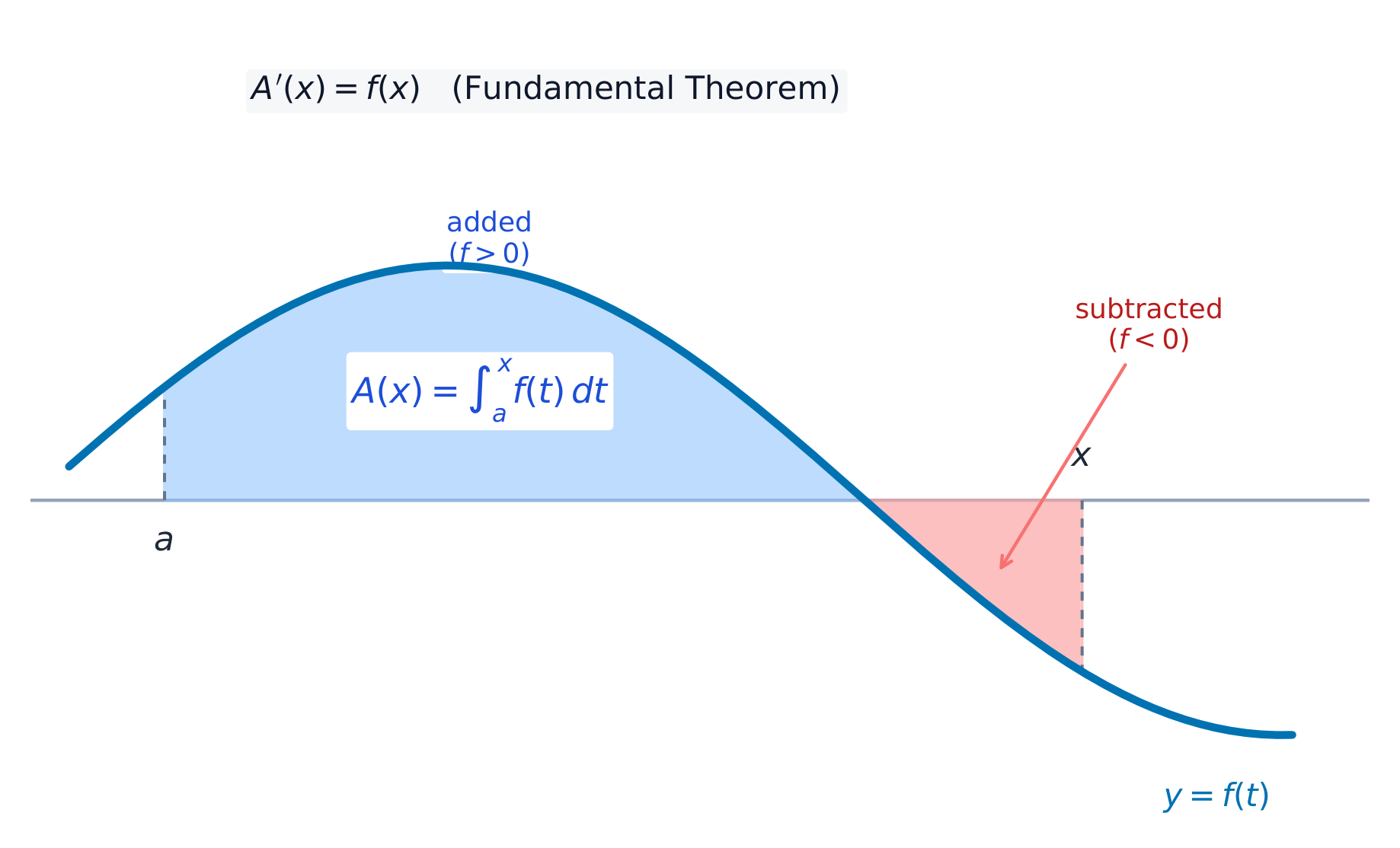
The Fundamental Theorem of Calculus A definite integral with a variable upper limit defines a new accumulation function 累积函数. The Fundamental Theorem of Calculus 微积分基本定理 (first part) says differentiation undoes this accumulation: if $f$ is continuous, then
$$\frac{d}{dx}\int_a^x f(t)\,dt = f(x).$$So if $g(x)=\int_a^x f(t)\,dt$, then $g'(x)=f(x)$ and $g''(x)=f'(x)$. This is the engine behind the very common "let $g(x)=\int_a^x f(t)\,dt$" questions.The accumulation function adds signed area; the FTC says its derivative is f 탐색하기적분을 통해 면적 축적하기
y = ax³ + bx² + cx + d
적분 함수 $\int_a^x f(t)\,dt$는 $x$이 이동함에 따라 부호 있는 면적이 쌓입니다. 기본 정리에 따르면 이 함수의 도함수는 단순히 $f(x)$입니다.
어휘 연습하기English 한국어 accumulation function/əˌkjuːmjʊˈleɪʃn ˈfʌŋkʃn/ 적분 함수 Fundamental Theorem of Calculus/ˌfʌndəˈmentl ˈθɪərəm ɒv ˈkælkjʊləs/ 미적분학 기본 정리 6.5
Behavior of Accumulation Functions
Syllabus
지속적 이해 (FUN-5): 미적분학의 기본 정리는 미분과 적분을 연결시킨다.
학습 목표 FUN-5.A: 정적분을 사용하여 적분 함수를 표현한다.
- FUN-5.A.3 함수 $f$의 그래프적, 수치적, 분석적 및 언어적 표현은 함수 $g$에 대한 정보를 제공하며, 이 함수는 $g(x) = \int_{a}^{x} f(t)\,dt$로 정의됩니다.
출처: College Board AP Course and Exam Description
Because $g'(x)=f(x)$, everything from Unit 5 applies to an accumulation function using the graph of $f$:
- $g$ is increasing where $f>0$ and decreasing where $f<0$;
- $g$ has a local extremum where $f$ crosses zero (with a sign change);
- $g$ is concave up where $f$ is increasing; inflection points of $g$ occur where $f$ has a local extremum.
To get a value of $g$, compute the signed area: $g(x)=\int_a^x f(t)\,dt$, adding areas above the axis and subtracting areas below.
6.6
Properties of Definite Integrals
Syllabus
지속적 이해 (FUN-6): 기하학적 지식과 수학적 규칙을 적용할 기회를 파악하면 적분이 단순화될 수 있다.
학습 목표 FUN-6.A: 면적과 정적분의 성질을 사용하여 정적분을 계산한다.
- FUN-6.A.1 일부 경우, 정적분은 기하학적 방법과 정적분 및 면적 간의 관계를 사용하여 계산할 수 있다.
- FUN-6.A.2 정적분의 성질로는 상수 times 함수의 적분, 두 함수의 합에 대한 적분, 적분 한계의 반전, 인접한 구간에서 한 함수의 적분이 포함된다.
- FUN-6.A.3 정적분의 정의는 제거 가능한 불연속점이나 점프 불연속점이 있는 함수로 확장될 수 있다.
출처: College Board AP Course and Exam Description
These properties simplify computation and appear constantly:
$$\int_a^a f = 0,\qquad \int_b^a f = -\int_a^b f,\qquad \int_a^b \big(f\pm g\big) = \int_a^b f \pm \int_a^b g,$$$$\int_a^b k\,f = k\int_a^b f,\qquad \int_a^c f + \int_c^b f = \int_a^b f.$$The last (splitting at an interior point $c$) lets you build a total integral from pieces read off a graph.6.7
The Fundamental Theorem and Evaluating Integrals
Syllabus
Enduring Understanding Learning Objective Essential Knowledge FUN-6
Recognizing opportunities to apply knowledge of geometry and mathematical rules can simplify integration.FUN-6.B
Evaluate definite integrals analytically using the Fundamental Theorem of Calculus.- FUN-6.B.1 An antiderivative of a function $f$ is a function $g$ whose derivative is $f$.
- FUN-6.B.2 If a function $f$ is continuous on an interval containing $a$, the function defined by $F(x) = \int_{a}^{x} f(t)\,dt$ is an antiderivative of $f$ for $x$ in the interval.
- FUN-6.B.3 If $f$ is continuous on the interval $[a, b]$ and $F$ is an antiderivative of $f$, then $\int_{a}^{b} f(x)\,dx = F(b) - F(a)$.
출처: College Board AP Course and Exam Description
The second part of the Fundamental Theorem evaluates a definite integral using an antiderivative 原函数. If $F'=f$, then
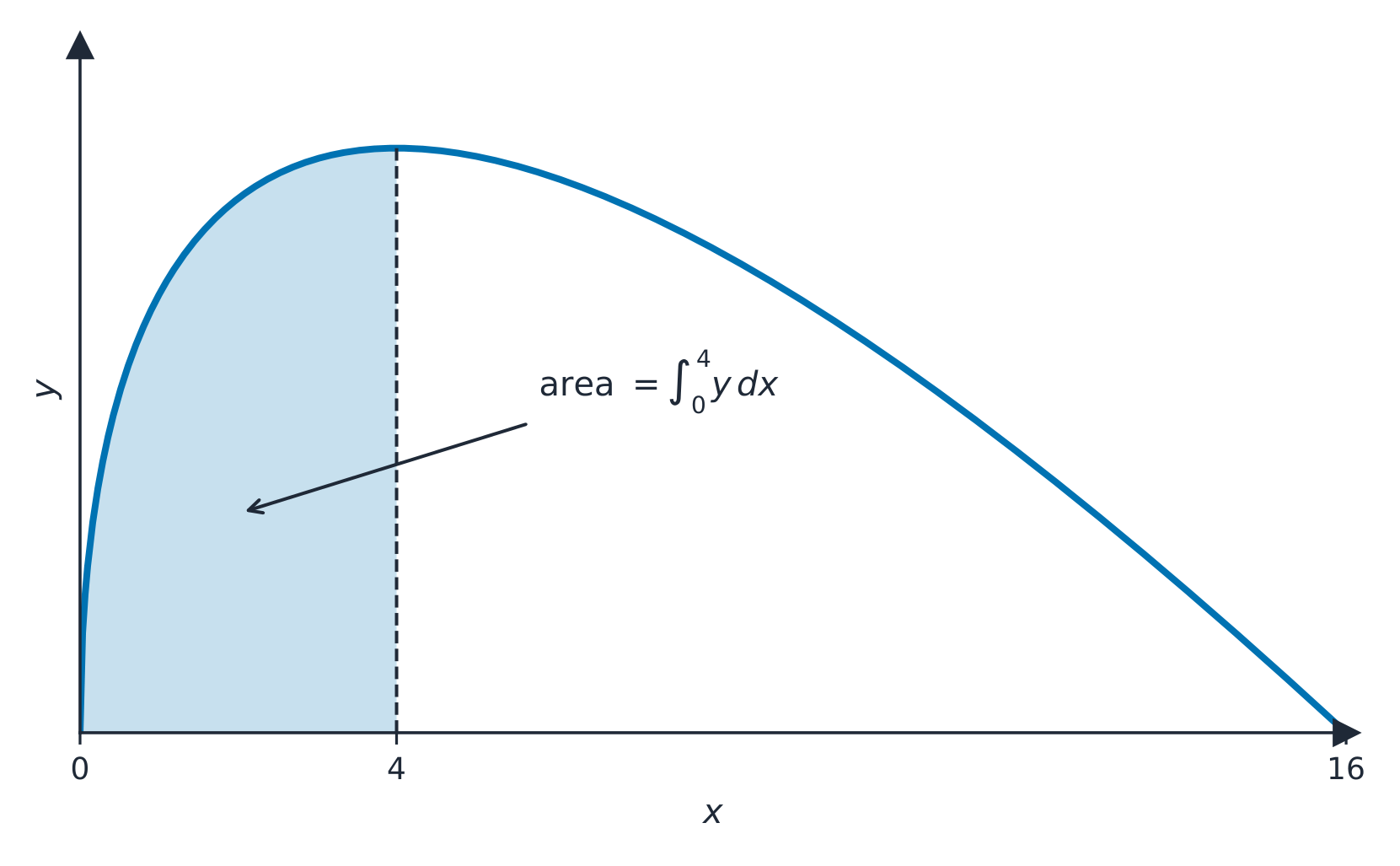
$$\int_a^b f(x)\,dx = F(b)-F(a).$$So: find any antiderivative $F$, then subtract its values at the two limits. This is how most exact integrals are computed. It also gives the net change view: $\int_a^b g'(t)\,dt = g(b)-g(a)$, so a starting value plus accumulated change gives a later value, e.g. $g(5)=g(0)+\int_0^5 g'(t)\,dt$.Worked example. Evaluate $\int_1^3 (2x+1)\,dx$. An antiderivative is $F(x)=x^2+x$, so
$$\int_1^3(2x+1)\,dx=F(3)-F(1)=(9+3)-(1+1)=12-2=10.$$A definite integral is the signed area between the curve and the x-axis 어휘 연습하기English 한국어 antiderivative/ˌæntɪdɪˈrɪvətɪv/ 원함수(alternative integral) 6.8
Antiderivatives and Indefinite Integrals
Syllabus
Enduring Understanding Learning Objective Essential Knowledge FUN-6
Recognizing opportunities to apply knowledge of geometry and mathematical rules can simplify integration.FUN-6.C
Determine antiderivatives of functions and indefinite integrals, using knowledge of derivatives.- FUN-6.C.1 $\int f(x)\,dx$ is an indefinite integral of the function $f$ and can be expressed as $\int f(x)\,dx = F(x) + C$, where $F'(x) = f(x)$ and $C$ is any constant.
- FUN-6.C.2 Differentiation rules provide the foundation for finding antiderivatives.
- FUN-6.C.3 Many functions do not have closed-form antiderivatives.
출처: College Board AP Course and Exam Description
An indefinite integral 不定积分 is the family of all antiderivatives, written with a constant of integration 积分常数:
$$\int f(x)\,dx = F(x)+C.$$Reverse each derivative rule to build the basic antiderivatives:$$\int x^n\,dx = \frac{x^{n+1}}{n+1}+C\ (n\neq -1),\quad \int \frac{1}{x}\,dx = \ln|x|+C,\quad \int e^x\,dx = e^x+C,$$$$\int \cos x\,dx = \sin x + C,\quad \int \sin x\,dx = -\cos x + C.$$어휘 연습하기English 한국어 indefinite integral/ɪnˈdefɪnət ˈɪntɪɡrəl/ 부정적분 constant of integration/ˈkɒnstənt ɒv ˌɪntɪˈɡreɪʃn/ 적분 상수 6.9
Integrating Using Substitution
Syllabus
지속적 이해 (FUN-6): 기하학적 지식과 수학적 규칙을 적용할 기회를 파악하면 적분이 단순화될 수 있다.
학습 목표 FUN-6.D: 치환이나 등가 형태로 변형이 필요한 피적분 함수에 대해: (a) 부정적분을 구하고, (b) 정적분을 계산한다.
- FUN-6.D.1 변수 치환은 원함수를 구하기 위한 기법이다.
- FUN-6.D.2 정적분에 대해 변수 치환을 할 때는 적분 범위의 대응적인 변경도 필요하다.
출처: College Board AP Course and Exam Description
$u$-substitution 换元积分法 reverses the chain rule. Choose an inside function $u=g(x)$, so $du=g'(x)\,dx$, and rewrite the integral entirely in $u$:
$$\int f\big(g(x)\big)g'(x)\,dx = \int f(u)\,du.$$Look for a function and its derivative both present. For a definite integral, either change the limits to $u$-values or convert back to $x$ before substituting the original limits.Worked example. Evaluate $\int 2x\cos(x^2)\,dx$. The inside function is $u=x^2$, whose derivative $2x\,dx=du$ is present, so
$$\int 2x\cos(x^2)\,dx=\int \cos u\,du=\sin u + C=\sin(x^2)+C.$$Spotting that $2x$ is exactly $\dfrac{du}{dx}$ is the whole trick.6.10
Long Division and Completing the Square
Syllabus
지속적 이해 (FUN-6): 기하학적 지식과 수학적 규칙을 적용할 기회를 파악하면 적분이 단순화될 수 있다.
학습 목표 FUN-6.D: 치환이나 등가 형태로 변형이 필요한 피적분 함수에 대해: (a) 부정적분을 구하고, (b) 정적분을 계산한다.
- FUN-6.D.3 원함수를 찾는 기법에는 등가 형태로 변형하는 방법이 포함되는데, 이를 위해 나눗셈이나 완전제곱식을 사용하기도 한다.
출처: College Board AP Course and Exam Description
Two algebraic set-up moves let more integrals fit the basic forms: polynomial long division 多项式长除法 when the top degree is $\ge$ the bottom degree of a rational function, and completing the square 配方法 to turn a quadratic denominator into a form that integrates to an arctangent or logarithm.
어휘 연습하기English 한국어 polynomial long division/ˌpɒlɪˈnəʊmɪəl lɒŋ dɪˈvɪʒn/ 다항식 장除法(長除法) completing the square/kəmˈpliːtɪŋ ðə skweə/ 완전제곱식 6.14
Selecting Techniques for Antidifferentiation
Syllabus
이 주제는 원함수 구法에 적합한 절차를 선택하는 능력에 초점을 맞춘 것이다. 학생들에게 원함수 구法 관련 모든 학습 목표를 언제, 어떻게 적용해야 하는지 연습할 기회가 제공되어야 한다.
출처: College Board AP Course and Exam Description
A skill topic: match the integral to a method. Try a basic antiderivative first; look for a $u$-substitution (an inside function whose derivative is also present); use algebra (division, completing the square, splitting a fraction) to reshape the integrand into a standard form. Naming the structure first prevents wasted effort.
6.14
Exam tips
- Integration is antidifferentiation; use the power rule $\int x^n\,dx=\tfrac{x^{n+1}}{n+1}+C$ and don't forget the $+C$.
- The Fundamental Theorem links the two: $\int_a^b f'(x)\,dx=f(b)-f(a)$, and $\tfrac{d}{dx}\int_a^x f(t)\,dt=f(x)$.
- Approximate a definite integral with Riemann sums or the trapezoidal rule from a table of values.
- A definite integral is a signed area (below the axis counts negative); split at sign changes for total area.
- Use u-substitution and remember to change the limits (or back-substitute) accordingly.
어휘 연습하기English 한국어 u-substitution/juː ˌsʌbstɪˈtjuːʃn/ u-대치法 -
7
미분방정식
수업 보기7.1
Modeling Situations with Differential Equations
Syllabus
지속적 이해(FUN-7): 미분 방정식을 풀면 함수를 결정하고 모델을 개발할 수 있다.
학습 목표 FUN-7.A: 도함수 식을 포함하는 미분 방정식으로 문제의 서술을 해석한다.
- FUN-7.A.1 미분 방정식은 독립 변수의 함수와 해당 함수의 도함수 사이의 관계를 나타낸다.
출처: College Board AP Course and Exam Description
A differential equation 微分方程 is an equation that relates a function to its own derivatives. It describes a situation by its rate of change. For example, "the rate of change of a quantity is proportional to its size" becomes
$$\frac{dy}{dt} = ky.$$Learning to translate a sentence about a rate into a differential equation is the first skill of this unit.어휘 연습하기English 한국어 differential equation/ˌdɪfəˈrenʃl ɪˈkweɪʒn/ 미분 방정식 7.2
Verifying Solutions for Differential Equations
Syllabus
지속적 이해(FUN-7): 미분 방정식을 풀면 함수를 결정하고 모델을 개발할 수 있다.
학습 목표 FUN-7.B: 미분 방정식의 해를 검증한다.
- FUN-7.B.1 도함수를 사용하여 주어진 함수가 특정 미분 방정식의 해임을 확인할 수 있다.
- FUN-7.B.2 미분 방정식의 일반해는 무한히 많을 수 있다.
출처: College Board AP Course and Exam Description
A solution 解 of a differential equation is a function that makes it true. You can verify a proposed solution by differentiating it and substituting into the equation: if both sides match, it is a solution. Note a differential equation usually has infinitely many solutions – a whole family – differing by a constant.
어휘 연습하기English 한국어 solution/səˈluːʃn/ 용액 7.3
Sketching Slope Fields

Syllabus
Enduring Understanding Learning Objective Essential Knowledge FUN-7
Solving differential equations allows us to determine functions and develop models.FUN-7.C
Estimate solutions to differential equations.- FUN-7.C.1 A slope field is a graphical representation of a differential equation on a finite set of points in the plane.
- FUN-7.C.2 Slope fields provide information about the behavior of solutions to first-order differential equations.
출처: College Board AP Course and Exam Description
Slope fields & solution curves A slope field 斜率场 draws the differential equation as a grid of short segments: at each point $(x,y)$ the segment has slope $\dfrac{dy}{dx}$ evaluated there. To sketch one, plug several points into the right-hand side and draw a small segment with that slope at each. The picture shows the shape of the solution curves without solving.
Each short segment has the slope $\dfrac{dy}{dx}$ at that point; a solution curve threads through, staying tangent to the field. Exam skill. A common part gives a portion of a slope field and asks you to sketch the particular solution through a given point – start at the point and follow the segments, staying tangent to them.
탐색하기미분방정식을 기울기 장으로 읽기
기울기 장은 각 점에서 기울기 $dy/dx$를 그려줍니다. 해 곡선이 작은 선분들을 항상 접하도록 관통하며, 흐름을 따라 그리면 손으로 스케치할 수 있습니다.
어휘 연습하기English 한국어 slope field/sləʊp fiːld/ 기울기 장 7.4
Reasoning Using Slope Fields
Syllabus
지속적 이해(FUN-7): 미분 방정식을 풀면 함수를 결정하고 모델을 개발할 수 있다.
학습 목표 FUN-7.C: 미분 방정식의 해를 추정한다.
- FUN-7.C.3 미분 방정식의 해는 함수 또는 함수族이다.
출처: College Board AP Course and Exam Description
Solutions to a differential equation are functions or families of functions. Read a slope field to reason about behavior: where the segments are flat ($\tfrac{dy}{dx}=0$) the solution is momentarily level; where they steepen the solution rises or falls faster; horizontal rows of equal slope suggest the rate depends only on $y$ (or only on $x$).
7.6
Finding General Solutions Using Separation of Variables
Syllabus
지속적 이해(FUN-7): 미분 방정식을 풀면 함수를 결정하고 모델을 개발할 수 있다.
학습 목표 FUN-7.D: 미분 방정식의 일반해를 구한다.
- FUN-7.D.1 일부 미분 방정식은 변수 분리법을 통해 풀 수 있다.
- FUN-7.D.2 원적분을 이용하여 미분 방정식의 일반해를 구할 수 있다.
출처: College Board AP Course and Exam Description
Many exam differential equations are solved by separation of variables 分离变量法. If $\dfrac{dy}{dx}$ factors into a function of $x$ times a function of $y$, move all $y$'s to one side and all $x$'s to the other, then integrate both sides:
$$\frac{dy}{dx}=g(x)h(y)\;\Longrightarrow\;\int \frac{dy}{h(y)} = \int g(x)\,dx.$$Add the constant of integration once (on the $x$-side). This gives the general solution 通解.Worked example. Solve $\dfrac{dy}{dx}=xy$ with the initial condition $y(0)=2$. Separate and integrate:
$$\int\frac{dy}{y}=\int x\,dx\;\Rightarrow\;\ln|y|=\frac{x^2}{2}+C\;\Rightarrow\;y=Ae^{x^2/2}.$$Applying $y(0)=2$ gives $A=2$, so the particular solution is $y=2e^{x^2/2}$.어휘 연습하기English 한국어 separation of variables/ˌsepəˈreɪʃn ɒv ˈveərɪəblz/ 변수 분리 general solution/ˈdʒenərəl səˈluːʃn/ 일반 해 7.7
Finding Particular Solutions Using Initial Conditions and Separation of Variables
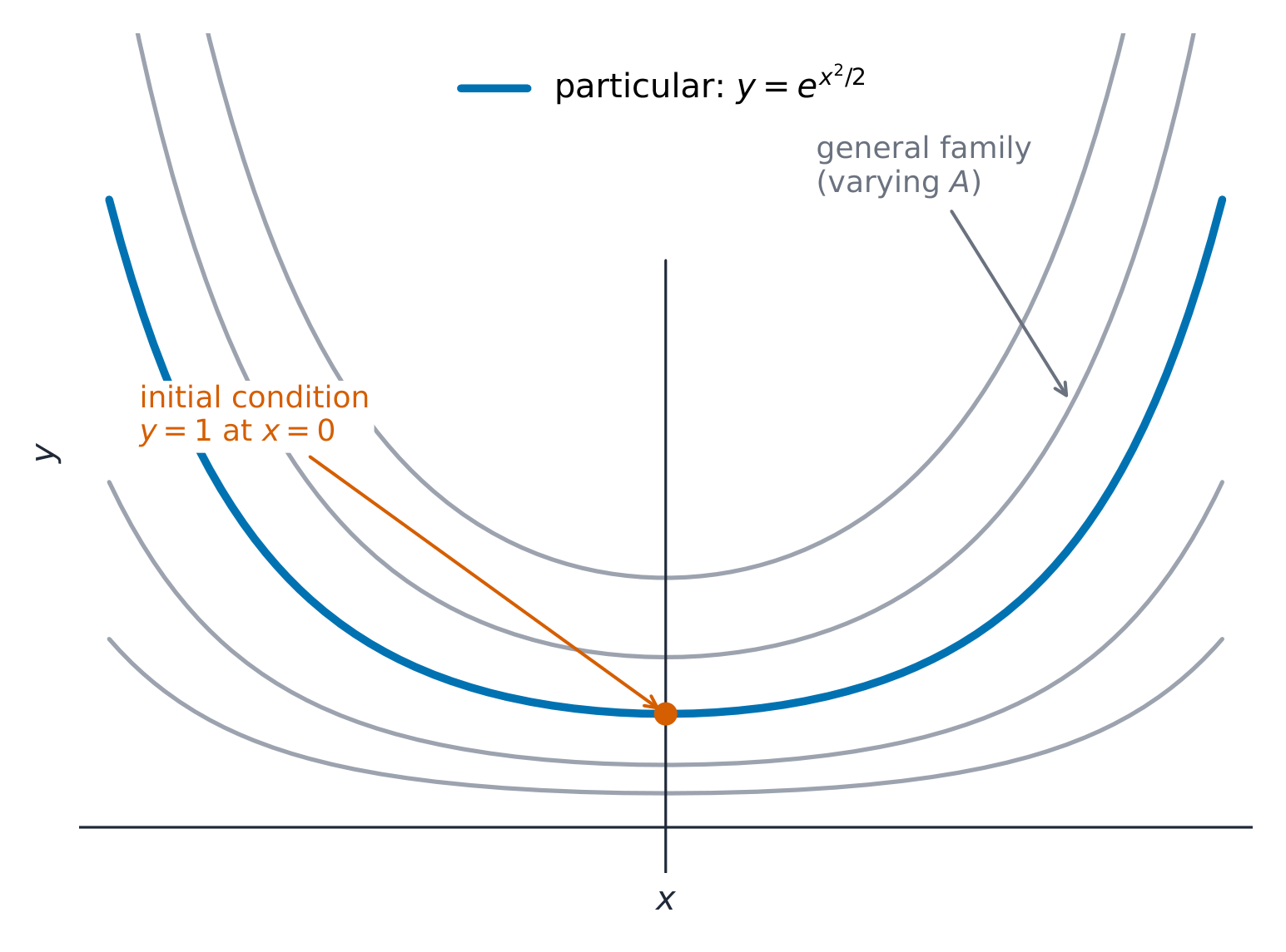
Syllabus
지속적 이해(FUN-7): 미분 방정식을 풀면 함수를 결정하고 모델을 개발할 수 있다.
학습 목표 FUN-7.E: 미분 방정식의 특이해를 구한다.
- FUN-7.E.1 일반해는 미분 방정식의 무한히 많은 해를 나타낼 수 있다. 주어진 점을 지나는 특이해는 오직 하나뿐이다.
- FUN-7.E.2 $F$로 정의된 함수 $F(x) = y_0 + \int_a^x f(t)\,dt$는 미분방정식 $\dfrac{dy}{dx} = f(x)$에 대한 특해이며, $F(a) = y_0$를 만족합니다.
- FUN-7.E.3 미분 방정식의 해는 정의역 제한을 받을 수 있다.
출처: College Board AP Course and Exam Description
An initial condition 初始条件 – a known point $(x_0,y_0)$ – pins down one curve from the family. Substitute it to solve for the constant $C$; the result is the particular solution 特解. There is exactly one solution through a given point. Watch for domain restrictions 定义域限制: keep the branch that contains the initial point (for example, the correct sign of a square root).
The constant gives a family of curves; an initial condition picks out one 어휘 연습하기English 한국어 initial condition/ɪˈnɪʃl kənˈdɪʃn/ 초기 조건 particular solution/pəˈtɪkjʊlə səˈluːʃn/ 특이해 domain restrictions/dəˈmeɪn rɪˈstrɪkʃnz/ 정의역 제한 7.8
Exponential Models with Differential Equations
Syllabus
지속적 이해(FUN-7): 미분 방정식을 풀면 함수를 결정하고 모델을 개발할 수 있다.
학습 목표 FUN-7.F: 문맥 속에서 미분 방정식과 그 변수의 의미를 해석한다.
- FUN-7.F.1 미분 방정식의 일반해와 특이해를 구하는 구체적인 응용 예로는 직선상에서의 운동과 지수적 성장 및 감쇠가 있다.
- FUN-7.F.2 "어떤 양의 변화율은 해당 양의 크기에 비례한다"는 서술로부터 도출되는 지수적 성장 및 감쇠 모델은 $\dfrac{dy}{dt} = ky$이다.
학습 목표 FUN-7.G: 문맥 속 미분 방정식 문제를 위한 일반해와 특이해를 구한다.
- FUN-7.G.1 지수 성장 및 감쇠 모델 $\dfrac{dy}{dt} = ky$에서 초기 조건이 $y = y_0$일 때($t = 0$), 이 미분방정식은 $y = y_0 e^{kt}$ 형태의 해를 가집니다.
출처: College Board AP Course and Exam Description
E. coli under a microscope: differential equations model exponential growth of populations The most important model is exponential growth and decay 指数增长与衰减. The equation $\dfrac{dy}{dt}=ky$ (rate proportional to size) has the solution:
$$y = y_0\,e^{kt},$$where $y_0$ is the value at $t=0$. Here $k>0$ gives growth and $k<0$ gives decay. You can derive this by separation of variables ($\int \tfrac{dy}{y} = \int k\,dt$), and it models processes like population growth, radioactive decay, and Newton's law of cooling. A follow-up part may ask for $\dfrac{d^2y}{dt^2}$: differentiate $\dfrac{dy}{dt}=ky$ again (using $\dfrac{dy}{dt}=ky$) to express it in terms of $y$.Worked example. A sample decays by $\dfrac{dy}{dt}=-0.10\,y$ (in years) from $y_0=50\ \text{g}$. The solution is $y=50e^{-0.10t}$, so after $10$ years $y=50e^{-1}=18.4\ \text{g}$. Its half-life solves $25=50e^{-0.10t}$, i.e. $e^{-0.10t}=\tfrac12$, giving $t=\dfrac{\ln 2}{0.10}=6.9\ \text{years}$ – independent of the starting amount.

A cooling cup of coffee: Newton's law of cooling is a classic differential equation model 탐색하기지수 성장/감쇠 모델
y = a·e^(bx) + c
방정식 $dy/dt=ky$의 해는 지수 함수입니다: 양은自身에 비례하는 속도로 변화하므로 무한 성장($k>0$)이나 0으로 수렴하는 감쇠($k<0$)를 보입니다.
어휘 연습하기English 한국어 exponential growth and decay/ˌekspəˈnenʃl ɡrəʊθ ænd dɪˈkeɪ/ 지수 성장 및 감쇠 7.8
Exam tips
- Solve a separable equation by getting all $y$ on one side and all $x$ on the other, then integrating both sides (add $+C$ once).
- Use the initial condition to find $C$ (a particular solution).
- Sketch or read a slope field: the little segments show $\tfrac{dy}{dx}$ at each point, and a solution curve follows them.
- Recognise exponential models $\tfrac{dy}{dt}=ky\Rightarrow y=Ce^{kt}$ (growth/decay).
- A differential equation gives the slope — you must integrate to recover the function.
-
8
적분의 적용
수업 보기8.1
함수의 평균값
Syllabus
지속적 이해 (CHA-4): 정적분은 구간 내에서의 변화량 축적 문제를 해결할 수 있게 해준다.
학습 목표 CHA-4.B: 정적분을 사용하여 함수의 평균값을 구한다.
- CHA-4.B.1 연속함수 $f$가 구간 $[a, b]$에서의 평균값은 $\dfrac{1}{b-a}\int_{a}^{b} f(x)\,dx$입니다.
출처: College Board AP Course and Exam Description
연속 함수 $f$의区间 $[a,b]$에서의 평균값은 적분을 구간 길이로 나눈 값입니다:
$$f_{\text{avg}} = \frac{1}{b-a}\int_a^b f(x)\,dx.$$이는区间 $[a,b]$ 위에서 함수 $f$ 아래 면적과 같은 직사각형의 일정한 높이를 의미합니다. 이를 변화의 평균율(변화량 *$f$*를 구간으로 나옴)이나 몇 개의 값에 대한 리만 합 평균과 혼동하지 마십시오. 시험에서는 이들을 명확히 구분합니다. 맥락에 맞는 단위를 표기하십시오(예: 차량당 시간당 평균율 "vehicles per hour").해설 예제. $f(x)=x^2$의 $[0,3]$에서의 평균 값은
$$f_{\text{avg}}=\frac{1}{3-0}\int_0^3 x^2\,dx=\frac{1}{3}\left[\frac{x^3}{3}\right]_0^3=\frac{1}{3}(9)=3.$$탐색하기함수의 평균값
y = ax³ + bx² + cx + d
$f$의 $[a,b]$에서의 평균값은 적분을 너비로 나눈 값으로, 곡선 아랫면적과 같은 면적을 가진 사각형의 일정 높이에 해당합니다.
8.2
적분을 이용한 위치, 속도, 가속도
Syllabus
지속적 이해 (CHA-4): 정적분은 구간 내에서의 변화량 축적 문제를 해결할 수 있게 해준다.
학습 목표 CHA-4.C: 직선 운동이 포함된 문제에서 정적분을 사용하여 위치와 변화율의 값을 구할 수 있다.
- CHA-4.C.1 시간 구간에서 직선 운동을 하는 입자에 대해, 속도의 정적분은 해당 시간 구간의 변위를 나타내며, 속력(steady speed)의 정적분은 해당 시간 구간의 이동 거리를 나타낸다.
출처: College Board AP Course and Exam Description
적분은 단원 4의 운동 링크를 반대로 만듭니다. 직선 운동을 하는 입자가 $[t_1,t_2]$ 구간 동안 이동할 때:
- 변위(displacement) (위치의 순변화) $= \displaystyle\int_{t_1}^{t_2} v(t)\,dt$.
- 이동한 총 거리 $= \displaystyle\int_{t_1}^{t_2} |v(t)|\,dt$ – 속력을 적분하여 방향 변화가 상쇄되지 않고 합산되게 합니다.
- 후속 시간 $= x(t_1) + \displaystyle\int_{t_1}^{t} v(s)\,ds$에서의 위치; 가속도 $= v(t_1)+\int a$으로부터의 속도.
절대값을 동반한 변위와 이동 거리의 차이는 전형적인 채점 포인트입니다.
어휘 연습하기English 한국어 average value/ˈævrɪdʒ ˈvæljuː/ 평균값 Displacement/dɪˈspleɪsmənt/ 치환 반응 Total distance travelled/ˈtəʊtl ˈdɪstəns ˈtrævld/ 이동한 총 거리 8.3
적용 맥락에서의 적분 함수와 정적분
Syllabus
지속적 이해 (CHA-4): 정적분은 구간 내에서의 변화량 축적 문제를 해결할 수 있게 해준다.
학습 목표 CHA-4.D: 적분 함수와 정적분을 사용하여 변화율을 적분하는 의미를 해석할 수 있다.
- CHA-4.D.1 적분으로 정의된 함수는 변화율의 적분(누적)을 나타낸다.
- CHA-4.D.2 어떤 양의 변화율(steady rate)의 정적분은 그 양에 대한 순변화(net change)를 주어진 구간에 대해 제공한다.
학습 목표 CHA-4.E: 응용 맥락에서 정적분을 사용하여 순변화를 구할 수 있다.
- CHA-4.E.1 정적분은 다양한 응용 맥락에서 누적과 순변화에 대한 정보를 표현하는 데 사용할 수 있다.
출처: College Board AP Course and Exam Description
적분으로 정의된 함수는 변화율을 축적합니다. **순변화 정리(net change theorem)**는 일상적인 도구입니다: 구간에서의 변화율에 대한 정적분은 해당 물량의 순변화를 줍니다:
$$\text{(final)} = \text{(initial)} + \int_a^b (\text{rate})\,dt.$$따라서 "$t=5$ 시점 수조에 있는 물의 양" = 초기 양 + $\int_0^5(\text{inflow}-\text{outflow})\,dt$입니다. 부호(나가는 것은 마이너스)와 단위를 주의하세요. 많은 다중 부분 FRQ는 이 개념을 기반으로 만들어지는데, 종종 "전체 ...를 구하는 적분 식을 쓰되 계산하지 마라"와 함께 나옵니다.어휘 연습하기English 한국어 net change/net tʃeɪndʒ/ 순변화 cross section/krɒs ˈsekʃn/ 단면 triangle/ˈtraɪæŋɡl/ 삼각형 semicircle/ˈsemɪsɜːkl/ 반원 8.4
곡선 사이의 면적 구하기 (x에 대한 함수)
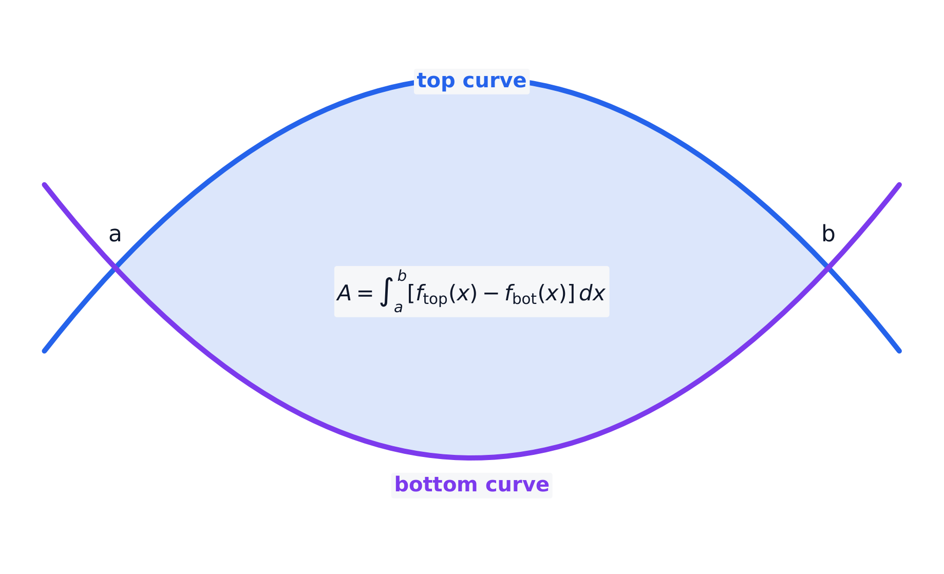
Syllabus
지속적 이해(CHA-5): 정적분은 구간에 따른 면적이나 부피의 누적 변화 관련 문제를 해결할 수 있게 한다.
학습 목표 CHA-5.A: 정적분을 사용하여 평면상의 면적을 계산할 수 있다.
- CHA-5.A.1 평면상의 영역의 면적은 정적분을 통해 계산할 수 있다.
출처: College Board AP Course and Exam Description
함수 $y=f(x)$(상단)와 $y=g(x)$(하단) 사이의 영역 면적은 $[a,b]$ 구간에서 다음과 같습니다:
$$A = \int_a^b \big[f(x)-g(x)\big]\,dx = \int_a^b (\text{top} - \text{bottom})\,dx.$$먼저 교차점을 찾아 적분 범위를 설정하고, 항상 아래쪽을 위쪽에서 뺍니다.해설 예시. $y=x$와 $y=x^2$ 사이의 면적을 구하십시오. 두 곡선은 $x=0$과 $x=1$에서 교차하며, $(0,1)$ 구간에서는 선 $y=x$이 위쪽에 있으므로
$$A=\int_0^1 (x-x^2)\,dx=\left[\frac{x^2}{2}-\frac{x^3}{3}\right]_0^1=\frac12-\frac13=\frac16.$$그림자 영역은 한 교점 $a$에서 다음 교점 $b$까지 이어지며, 그 면적은 $\int_a^b(\text{top}-\text{bottom})\,dx$입니다. 8.5
곡선 사이의 면적 구하기 (y에 대한 함수)
Syllabus
지속적 이해(CHA-5): 정적분은 구간에 따른 면적이나 부피의 누적 변화 관련 문제를 해결할 수 있게 한다.
학습 목표 CHA-5.A: 정적분을 사용하여 평면상의 면적을 계산할 수 있다.
- CHA-5.A.2 평면상의 영역의 면적은 x-함수나 y-함수를 사용하여 계산할 수 있다. $x$ $y$
출처: College Board AP Course and Exam Description
일부 영역은 수평slice로 설명하는 것이 더 쉽습니다: $y$에 대해 적분하십시오:
$$A = \int_c^d \big[x_{\text{right}}(y) - x_{\text{left}}(y)\big]\,dy = \int_c^d (\text{right}-\text{left})\,dy.$$전체 영역에 걸쳐 단일한 위/아래(또는 좌/우) 쌍을 유지하도록 $x$-slice 또는 $y$-slice를 선택하십시오.8.6
교차가 두 번 이상인 곡선 사이의 면적
Syllabus
지속적 이해(CHA-5): 정적분은 구간에 따른 면적이나 부피의 누적 변화 관련 문제를 해결할 수 있게 한다.
학습 목표 CHA-5.A: 정적분을 사용하여 평면상의 면적을 계산할 수 있다.
- CHA-5.A.3 평면상의 특정 영역의 면적은 두 개 이상의 정적분의 합으로 계산하거나 두 함수의 차이의 절댓값의 정적분을 평가하여 구할 수 있다.
출처: College Board AP Course and Exam Description
곡선이 두 번 이상 교차하면, 특정 구간에서는 한 함수가 위쪽에 있고 다른 구간에서는 다른 함수가 위쪽에 있습니다. 각 교차점에서 적분의 합으로 나누거나 차이의 절댓값을 적분하십시오:
$$A = \int_a^b \big|f(x)-g(x)\big|\,dx.$$적분을 쓰기 전에 각 하위 구간에서 어떤 곡선이 높은지 확인하십시오.8.7
단면이 정사각형 및 직사각형인 부피

Syllabus
지속적 이해(CHA-5): 정적분은 구간에 따른 면적이나 부피의 누적 변화 관련 문제를 해결할 수 있게 한다.
학습 목표 CHA-5.B: 알려진 단면을 가진 입체의 부피를 정적분을 사용하여 계산할 수 있다.
- CHA-5.B.1 정사각형 및 직사각형 단면을 가진 입체의 부피는 정적분과 해당 도형의 면적 공식으로 구할 수 있다.
출처: College Board AP Course and Exam Description
도자기 장인이 용기를 만들다: 회전 입체는 평면 영역을 회전시켜 형성되는 부피입니다 입체에 축에 수직인 알려진 단면이 있다면, 그 부피는 단면 면적의 적분입니다.
$$V = \int_a^b A(x)\,dx.$$정사각형 단면의 한 변이 영역의 높이 $s(x)=f(x)-g(x)$인 경우, $A(x)=[s(x)]^2$를 사용합니다. 높이가 $k\cdot s(x)$인 직사각형 단면의 경우, $A(x)=k\,[s(x)]^2$을 사용합니다. 고사 문제에서 "고체의 밑면...단면은 정사각형/직사각형"이라는 표현은 정확히 이 내용을 의미합니다.8.8
단면을 이용한 부피: 삼각형과 반원
Syllabus
지속적 이해(CHA-5): 정적분은 구간에 따른 면적이나 부피의 누적 변화 관련 문제를 해결할 수 있게 한다.
학습 목표 CHA-5.B: 알려진 단면을 가진 입체의 부피를 정적분을 사용하여 계산할 수 있다.
- CHA-5.B.2 삼각형 단면을 가진 입체의 부피는 정적분과 해당 도형의 면적 공식으로 구할 수 있다.
- CHA-5.B.3 반원 및 기타 기하학적으로 정의된 단면을 가진 입체의 부피는 정적분과 해당 도형의 면적 공식으로 구할 수 있다.
- *CHA-5.B.3 참고 예시:
- 단면이 원인 깔대기의 부피는 원의 면적 공식과 정적분을 사용하여 구할 수 있다 (2016 AB Exam FRQ #5(b) 참조).
- 단면적(steady area)이 함수로 정의된 입체의 부피는 알려진 면적(steady area) 함수와 정적분을 사용하여 구할 수 있다 (2009 AB Exam FRQ #4(c) 참조).
- *CHA-5.B.3 참고 예시:
출처: College Board AP Course and Exam Description
같은 방법이지만 다른 면적 공식입니다. 한 변의 길이가 $s$인 정삼각형의 경우, $A=\tfrac{\sqrt{3}}{4}s^2$; 지름이 $s$인 반원의 경우, $A=\tfrac{\pi}{8}s^2$입니다. 도형의 주요 길이를 영역의slice 길이 $s(x)$와 같게 설정한 후, $A(x)$에 대해 적분합니다.
8.9
원판법(Disc Method)을 이용한 부피 (x축 또는 y축 기준)
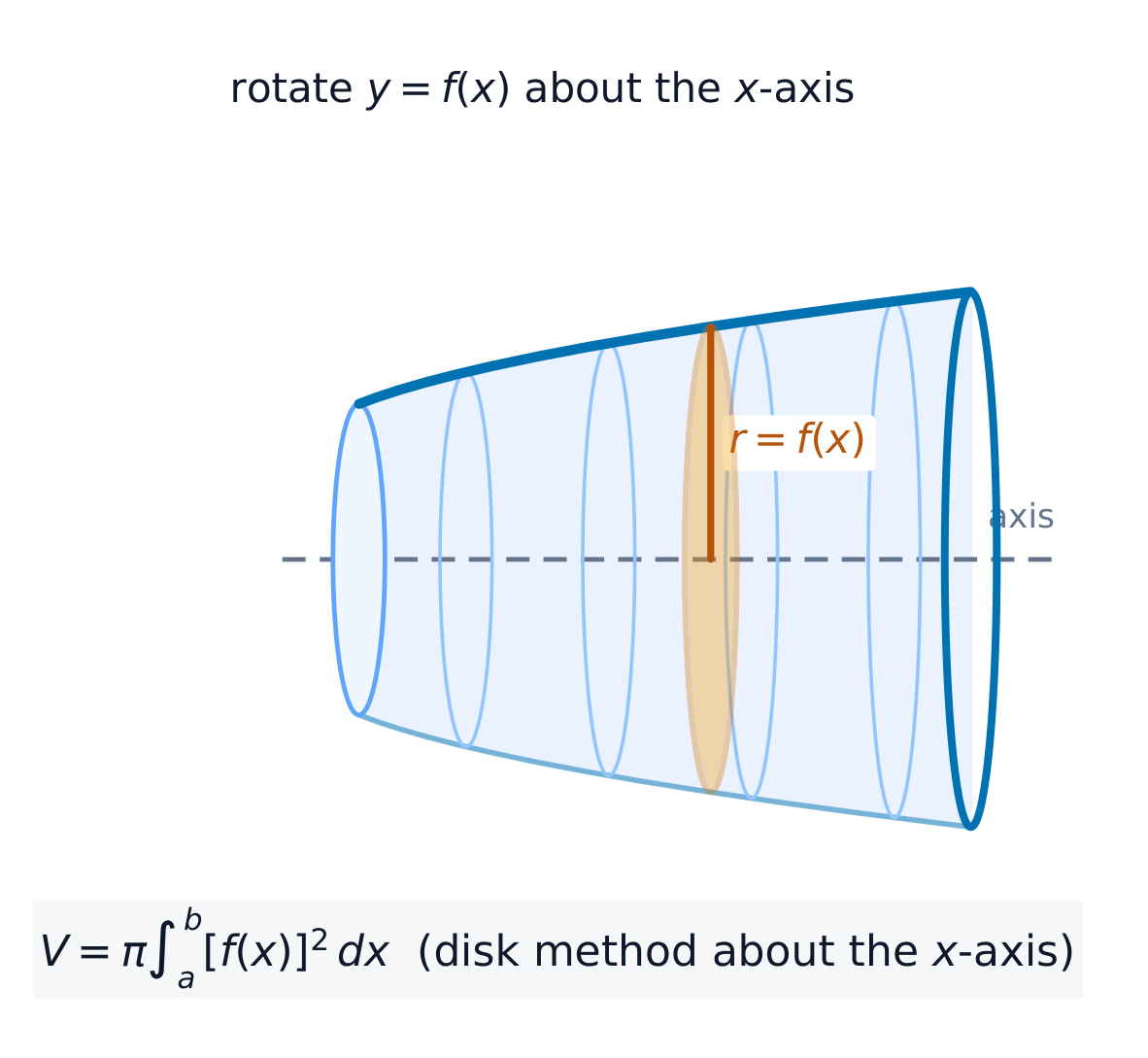
Syllabus
지속적 이해(CHA-5): 정적분은 구간에 따른 면적이나 부피의 누적 변화 관련 문제를 해결할 수 있게 한다.
학습 목표 CHA-5.C: 정적분을 사용하여 회전체의 부피를 계산한다.
- CHA-5.C.1 x축 또는 y축周围的人回전 입체의 부피는 원반법을 사용하여 정적분으로 구할 수 있다. $x$ $y$
출처: College Board AP Course and Exam Description
회전체: 원판법 영역을 축에 대해 회전하면 회전체가 됩니다. 영역이 축에 닿아 있다면, 각 slice는 반지름이 $r$ = 함수 값인 원판이 됩니다:
$$V = \pi\int_a^b [r(x)]^2\,dx.$$$x$축에 대해 회전할 때는 $r=f(x)$를 사용하고 $x$에 대해 적분하며, $y$축에 대해 회전할 때는 $x$를 $y$의 함수로 표현하여 $y$에 대해 적분합니다.원판법: y=f(x)를 축에 대해 회전하면 반지름이 f(x)인 원판이 생깁니다 해설 예제. $y=\sqrt{x}$ 아래 영역을 $x=0$부터 $x=4$까지 $x$축에 대해 회전합니다. 각 원판의 반지름은 $r=\sqrt{x}$이므로,
$$V=\pi\int_0^4 (\sqrt{x})^2\,dx=\pi\int_0^4 x\,dx=\pi\left[\frac{x^2}{2}\right]_0^4=8\pi.$$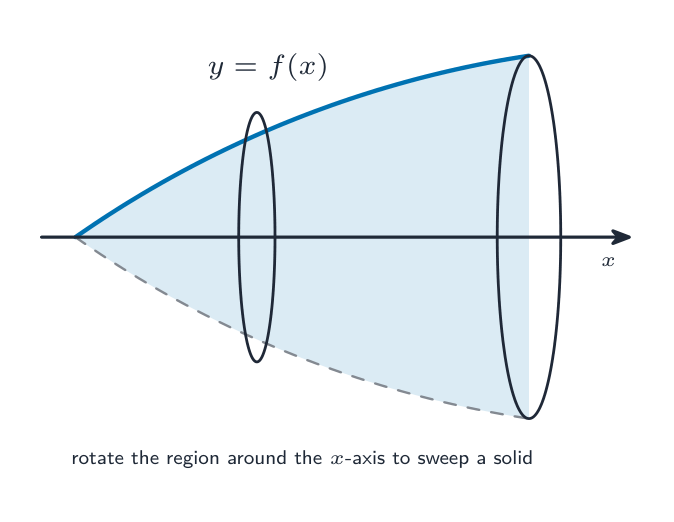
영역을 축에 대해 회전하면 회전체가 생깁니다 어휘 연습하기English 한국어 solid of revolution/ˈsɒlɪd ɒv ˌrevəˈluːʃn/ 회전체 disc/dɪsk/ 원판 8.10
원판법을 이용한 부피 (다른 축 기준)
Syllabus
지속적 이해(CHA-5): 정적분은 구간에 따른 면적이나 부피의 누적 변화 관련 문제를 해결할 수 있게 한다.
학습 목표 CHA-5.C: 정적분을 사용하여 회전체의 부피를 계산한다.
- CHA-5.C.2 평면상의 모든 수평선 또는 수직선을 중심으로 회전하는 회전체의 부피는 원반법과 정적분을 사용하여 구할 수 있다.
출처: College Board AP Course and Exam Description
어떤 수평선 또는 수직선 $y=k$ 또는 $x=k$에 대해 회전할 때, 반지름은 곡선에서 해당 직선까지의 거리입니다. 예를 들어 $r(x)=|f(x)-k|$입니다. 반지름을 주의 깊게 설정한 후, $V=\pi\int r^2$을 적용합니다.
8.11 8.12
와셔법(Washer Method)을 이용한 부피
Syllabus
지속적 이해(CHA-5): 정적분은 구간에 따른 면적이나 부피의 누적 변화 관련 문제를 해결할 수 있게 한다.
학습 목표 CHA-5.C: 정적분을 사용하여 회전체의 부피를 계산한다.
- CHA-5.C.3 $x$축 또는 $y$축을 중심으로 회전하며 단면이 고리 모양인 회전체의 부피는 와셔법과 정적분을 사용하여 구할 수 있다.
지속적 이해(CHA-5): 정적분은 구간에 따른 면적이나 부피의 누적 변화 관련 문제를 해결할 수 있게 한다.
학습 목표 CHA-5.C: 정적분을 사용하여 회전체의 부피를 계산한다.
- CHA-5.C.4 평면상의 모든 수평선 또는 수직선을 중심으로 회전하며 단면이 고리 모양인 회전체의 부피는 와셔법과 정적분을 사용하여 구할 수 있다.
출처: College Board AP Course and Exam Description
와셔법을 이용한 부피 영역이 축에 닿아 있지 않을 때, 각 slice는 외반지름이 $R$이고 내반지름이 $r$인 와셔(링 모양)가 됩니다:
$$V = \pi\int_a^b \Big([R]^2 - [r]^2\Big)\,dx.$$$R$는 축에서 더 멀리 있는 경계까지의 거리이며, $r$는 더 가까운 경계까지의 거리입니다. 축이 아닌 다른 직선에 대해 회전할 때에도 두 반지름은 모두 해당 직선까지의 거리로 측정됩니다. 이는 매우 흔한 고사 변형 문제입니다(예: $y=-2$축에 대해 회전).어휘 연습하기English 한국어 washer/ˈwɒʃə/ 와셔(링 반지름) 8.11 8.12
시험 팁
- 곡선 사이의 면적은 $\int(\text{top}-\text{bottom})\,dx$입니다 — 적분 구간의 경계점(교점)을구하고 상단 minus 하단을 유지하십시오.
- 회전체의 부피를 구하려면 면적이 $\pi r^2$인 원판/와셔 단면을 모두 더하거나(또는 $\pi(R^2-r^2)$), 적분합니다.
- $f$의 $[a,b]$ 구간에서의 평균값은 $\tfrac{1}{b-a}\int_a^b f\,dx$입니다.
- 누적 변화량은 속도의 $\int$입니다: 총량 = 초기 값 $+\int_a^b(\text{rate})\,dt$ + 적분값.
- 적분은 "무한히 작은 조각들을 모두 더하는 것"을 의미합니다 — 피적분식을 하나의 얇은 slice로 설정하십시오.