| Enduring Understanding | Learning Objective | Essential Knowledge |
|---|---|---|
CHA-1 | CHA-1.A |
|
Limits and Continuity
AP Calculus AB · Topic 1
 16:16
16:16
Limits & Continuity
Here is a puzzle. A car's speedometer reads sixty kilometres per hour. But what does speed mean at a single instant? Speed is distance divided by time. Yet at…
English narration · English + 中文 subtitles burned in
1.1
Introducing Calculus: Can Change Occur at an Instant?
Syllabus
Source: College Board AP Course and Exam Description
Calculus is the mathematics of change 变化 and of accumulation 累积. It answers two big questions: how fast is something changing right now, and how much has piled up so far? Unit 1 builds the one tool both questions rest on – the limit 极限.
Start with a puzzle. A car's speedometer reads $60$ km/h. What does that mean at a single instant 瞬间? Speed is distance over time. But at one instant no time passes and no distance is covered, so the fraction looks like $\tfrac{0}{0}$ – undefined.
- The average rate of change 平均变化率 uses a whole interval 区间: the change in one quantity divided by the change in another. It divides by zero, and so is undefined, when the change in the input would be zero.
- The instantaneous rate of change 瞬时变化率 is what we want at a point. It is the value the average rate approaches 趋近 as the interval shrinks toward zero length.
The clever move is not to plug in zero (undefined), but to watch what the average rate approaches as the interval gets smaller and smaller. That approaching value is a limit. So calculus lets us describe change at an instant – as a limit of average rates over ever-shorter intervals. This one idea powers the derivative 导数 (Unit 2) and, run in reverse, the integral 积分 (Unit 6). Everything else in this unit defines limits carefully and computes them reliably.
Explore
Explore rate of change at an instant
y = ax³ + bx² + cx + d
Slide the point along the curve. The tangent line is the limit of ever-shorter average rates — its slope is the instantaneous rate of change $\frac{dy}{dx}$ at that point.
Vocabulary
Train
| English |
|---|
| change/tʃeɪndʒ/ |
| accumulation/əˌkjuːmjʊˈleɪʃn/ |
| limit/ˈlɪmɪt/ |
| at a single instant/ætə ˈsɪŋɡl ˈɪnstənt/ |
| average rate of change/ˈævrɪdʒ reɪt ɒv tʃeɪndʒ/ |
| interval/ˈɪntəvl/ |
| instantaneous rate of change/ˌɪnstənˈteɪnɪəs reɪt ɒv tʃeɪndʒ/ |
| approaches/əˈprəʊtʃɪz/ |
| derivative/dɪˈrɪvətɪv/ |
| integral/ˈɪntɪɡrəl/ |
| hole/həʊl/ |
1.2
Defining Limits and Using Limit Notation

Syllabus
| Enduring Understanding | Learning Objective | Essential Knowledge |
|---|---|---|
LIM-1 | LIM-1.A |
|
LIM-1.B |
|
Source: College Board AP Course and Exam Description
Given a function $f$, the limit of $f(x)$ as $x$ approaches $c$ is a real number $R$ if $f(x)$ can be made arbitrarily 任意地 close to $R$ by taking $x$ sufficiently 足够 close to $c$ – but not equal to $c$. We write
$$\lim_{x \to c} f(x) = R$$
and read it: "the limit of $f(x)$, as $x$ approaches $c$, equals $R$."
The last words are the heart of a limit: it describes the behavior 行为 of $f$ near $c$, not the value at $c$. The function may be undefined at $c$, or defined but equal to something else – the limit does not care.
A limit can be shown in three ways: graphically 用图象, numerically 用数值 (a table), and analytically 用解析式 (algebra). Learning to move between these representations is a core skill.
(Note: the epsilon-delta definition of a limit is not tested on the AP Exam, so this handout does not use it.)
Vocabulary
Train
| English |
|---|
| arbitrarily/ˌɑːbɪˈtrerɪli/ |
| sufficiently/səˈfɪʃəntli/ |
| behavior/bɪˈheɪvjə/ |
| graphically/ˈɡræfɪkli/ |
| numerically/njuːˈmerɪkli/ |
| analytically/ˌænəˈlɪtɪkli/ |
1.3
Estimating Limit Values from Graphs
Syllabus
| Enduring Understanding | Learning Objective | Essential Knowledge |
|---|---|---|
LIM-1 | LIM-1.C |
|
Source: College Board AP Course and Exam Description
A graph is often the fastest way to read a limit. To find $\displaystyle \lim_{x \to c} f(x)$, run your finger along the curve toward $x = c$ from each side and ask: what height is the curve heading for?
- Trace from the left (inputs smaller than $c$): this gives the left-hand limit 左极限, $\displaystyle \lim_{x \to c^-} f(x)$.
- Trace from the right (inputs larger than $c$): this gives the right-hand limit 右极限, $\displaystyle \lim_{x \to c^+} f(x)$.
- These are the one-sided limits 单侧极限. If both head to the same height $R$, then the two-sided limit exists and $\displaystyle \lim_{x \to c} f(x) = R$.
Crucially, ignore the point itself. Graphs mark the difference between the limit and the value:
- An open circle 空心圆 marks a height the curve approaches but does not reach – a "hole" 空洞.
- A closed circle 实心圆 marks the actual value $f(c)$.
A limit does not exist (often written DNE) when the two sides disagree (a jump 跳跃), when the function is unbounded 无界 (grows without limit), or when it oscillates 振荡 forever near $c$. For example:
$$\lim_{x \to 0} \frac{1}{x^2} = \infty, \qquad \lim_{x \to 0} \frac{|x|}{x}\ \text{DNE}, \qquad \lim_{x \to 0} \sin\!\left(\frac{1}{x}\right)\ \text{DNE}.$$
Watch the scale 比例 of a graph: a zoomed-out picture can hide important behavior near a point, so confirm with algebra when you can.
Worked comparison: nearby values and one point
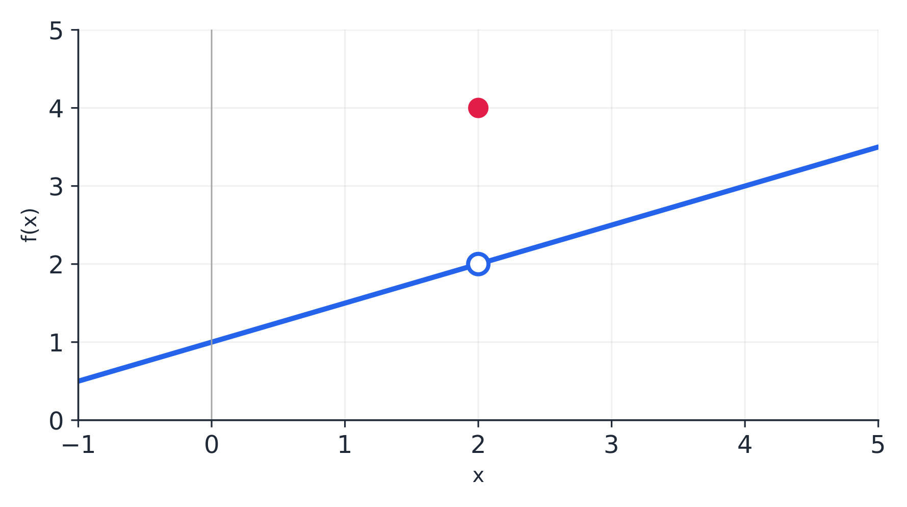
In this teacher-created graph, read the approaching heights before the filled point.
Both one-sided limits at 2 equal 2, so the two-sided limit is 2. The filled point gives $f(2)=4$. This is a removable discontinuity: set $f(2)=2$ to make the function continuous.
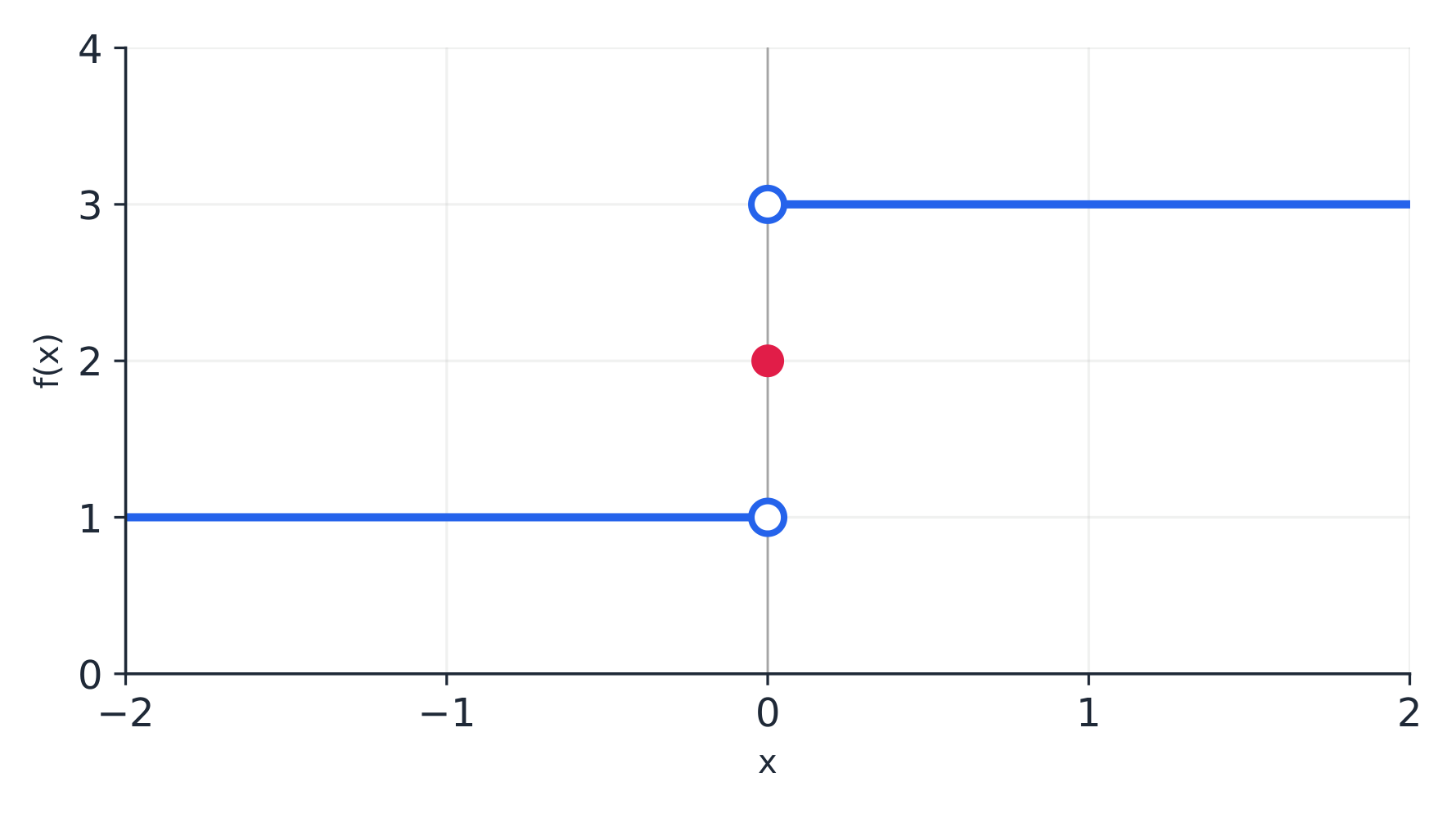
Here the left-hand limit at 0 is 1, the right-hand limit is 3, and $f(0)=2$. The unequal one-sided limits mean the two-sided limit does not exist. No choice of $f(0)$ changes the nearby branches; the jump cannot be removed by changing one point.
Explore
Read a limit off the graph
y = ax² + bx + c
The limit as $x\to c$ is the height the curve heads toward from both sides — it is about where the function is going, not its value at $c$. Follow the curve toward an $x$ and read the $y$ it approaches.
Vocabulary
Train
| English |
|---|
| left-hand limit/left hænd ˈlɪmɪt/ |
| right-hand limit/raɪt hænd ˈlɪmɪt/ |
| one-sided limits/wʌn ˈsaɪdɪd ˈlɪmɪts/ |
| open circle/ˈəʊpən ˈsɜːkl/ |
| closed circle/kləʊzd ˈsɜːkl/ |
| jump/dʒʌmp/ |
| unbounded/ʌnˈbaʊndɪd/ |
| oscillates/ˈɒsɪleɪts/ |
| scale/skeɪl/ |
1.4
Estimating Limit Values from Tables
Syllabus
| Enduring Understanding | Learning Objective | Essential Knowledge |
|---|---|---|
LIM-1 | LIM-1.C |
|
Source: College Board AP Course and Exam Description
When you have data or a formula but no picture, a table 表格 of values estimates a limit numerically. Choose inputs that creep toward $c$ from both sides and watch the outputs.
For example, to estimate $\displaystyle \lim_{x \to 2} \frac{x^2 - 4}{x - 2}$ (which is $\tfrac{0}{0}$ at $x=2$):
| $x$ | $1.9$ | $1.99$ | $1.999$ | $\to 2 \leftarrow$ | $2.001$ | $2.01$ | $2.1$ |
|---|---|---|---|---|---|---|---|
| $f(x)$ | $3.9$ | $3.99$ | $3.999$ | ? | $4.001$ | $4.01$ | $4.1$ |
Both sides march toward $4$, so we estimate the limit is $4$. A table only suggests a value – it is a numerical estimate, not a proof.
Vocabulary
Train
| English |
|---|
| table/ˈteɪbl/ |
1.5
Determining Limits Using Algebraic Properties of Limits
Syllabus
| Enduring Understanding | Learning Objective | Essential Knowledge |
|---|---|---|
LIM-1 | LIM-1.D |
|
Source: College Board AP Course and Exam Description
Most limits are found analytically using limit theorems 极限定理. If $\lim_{x\to c} f(x)$ and $\lim_{x\to c} g(x)$ both exist, the limit of a combination is the same combination of the limits:
- Sum / difference: $\displaystyle \lim_{x\to c}\big[f(x)\pm g(x)\big] = \lim_{x\to c}f(x) \pm \lim_{x\to c}g(x)$
- Product: $\displaystyle \lim_{x\to c}\big[f(x)\,g(x)\big] = \lim_{x\to c}f(x)\cdot\lim_{x\to c}g(x)$
- Quotient: $\displaystyle \lim_{x\to c}\frac{f(x)}{g(x)} = \frac{\lim_{x\to c}f(x)}{\lim_{x\to c}g(x)}$, provided the bottom limit is not $0$.
- Composite 复合函数: if $g$ is continuous at $\lim_{x\to c} f(x)$, then $\displaystyle \lim_{x\to c} g\big(f(x)\big) = g\!\left(\lim_{x\to c} f(x)\right)$.
The practical rule: for a function built from polynomials, roots, and the like, first try direct substitution 直接代入 – put $x = c$ in. If you get a real number, that is the limit. One-sided limits obey the same theorems, read from one direction only.
Vocabulary
Train
| English |
|---|
| limit theorems/ˈlɪmɪt ˈθɪərəmz/ |
| Composite/ˈkɒmpəzɪt/ |
| direct substitution/daɪˈrekt ˌsʌbstɪˈtjuːʃn/ |
1.6
Determining Limits Using Algebraic Manipulation
Syllabus
| Enduring Understanding | Learning Objective | Essential Knowledge |
|---|---|---|
LIM-1 | LIM-1.E |
|
Source: College Board AP Course and Exam Description
Direct substitution sometimes gives the indeterminate form 未定式 $\tfrac{0}{0}$. This does not mean the limit fails – it means you must rewrite the function into an equivalent form 等价形式 that removes the trouble, then substitute. Three standard moves:
- Factor and cancel 因式分解并约分 a rational function 有理函数. Example: $\displaystyle \lim_{x\to 2}\frac{x^2-4}{x-2} = \lim_{x\to 2}\frac{(x-2)(x+2)}{x-2} = \lim_{x\to 2}(x+2) = 4$.
- Multiply by the conjugate 共轭 to simplify a radical 根式. Example: $\displaystyle \lim_{x\to 0}\frac{\sqrt{x+1}-1}{x} = \lim_{x\to 0}\frac{x}{x\big(\sqrt{x+1}+1\big)} = \frac{1}{2}$.
- Use alternate forms of trigonometric functions (identities) to simplify.
The cancelled factor is why the original graph had a hole: the two functions agree everywhere except at $x=c$, so they share the same limit there.
Vocabulary
Train
| English |
|---|
| indeterminate form/ˌɪndɪˈtɜːmɪnət fɔːm/ |
| equivalent form/ɪˈkwɪvələnt fɔːm/ |
| Factor and cancel/ˈfæktə ænd ˈkænsl/ |
| rational function/ˈræʃənl ˈfʌŋkʃn/ |
| conjugate/ˈkɒndʒuːɡeɪt/ |
| radical/ˈrædɪkl/ |
1.7
Selecting Procedures for Determining Limits
Syllabus
This topic is intended to focus on the skill of selecting an appropriate procedure for determining limits. Students should be given opportunities to practice when and how to apply all learning objectives relating to determining limits.
Source: College Board AP Course and Exam Description
This is a skill topic, not new content: choose the right tool for the limit in front of you.
- Try direct substitution first. A real answer means you are done.
- Getting $\tfrac{0}{0}$? Rewrite – factor and cancel, or use the conjugate, or a trig identity – then substitute.
- A non-zero number over $0$ (like $\tfrac{5}{0}$)? The limit is infinite or DNE – check the sign from each side (see vertical asymptotes below).
- As $x\to\pm\infty$? Compare the dominant 主导 terms (see limits at infinity).
- Trapped between two functions? The squeeze theorem may apply.
Vocabulary
Train
| English |
|---|
| dominant/ˈdɒmɪnənt/ |
1.8
Determining Limits Using the Squeeze Theorem

Syllabus
| Enduring Understanding | Learning Objective | Essential Knowledge |
|---|---|---|
LIM-1 | LIM-1.E |
|
Source: College Board AP Course and Exam Description
The squeeze theorem 夹逼定理 (also called the sandwich theorem) finds a limit by trapping the function between two others. If $g(x) \le f(x) \le h(x)$ near $c$, and
$$\lim_{x\to c} g(x) = \lim_{x\to c} h(x) = L,$$
then $f$ is squeezed to the same place: $\displaystyle \lim_{x\to c} f(x) = L$.
The two famous results proved this way, both used throughout calculus, are:
$$\lim_{x\to 0}\frac{\sin x}{x} = 1 \qquad\text{and}\qquad \lim_{x\to 0}\frac{1-\cos x}{x} = 0.$$
Vocabulary
Train
| English |
|---|
| squeeze theorem/skwiːz ˈθɪərəm/ |
1.9
Connecting Multiple Representations of Limits
Syllabus
This topic is intended to focus on connecting representations. Students should be given opportunities to practice when and how to apply all learning objectives relating to limits and translating mathematical information from a single representation or across multiple representations.
Source: College Board AP Course and Exam Description
Another skill topic: the same limit lives in a graph, a table, and an algebraic form, and you should be able to translate between them. A graph shows the shape and any holes or jumps; a table gives numerical evidence; algebra gives an exact value and a reason. Strong answers use one representation to confirm another.
1.10
Exploring Types of Discontinuities
Syllabus
| Enduring Understanding | Learning Objective | Essential Knowledge |
|---|---|---|
LIM-2 | LIM-2.A |
|
Source: College Board AP Course and Exam Description
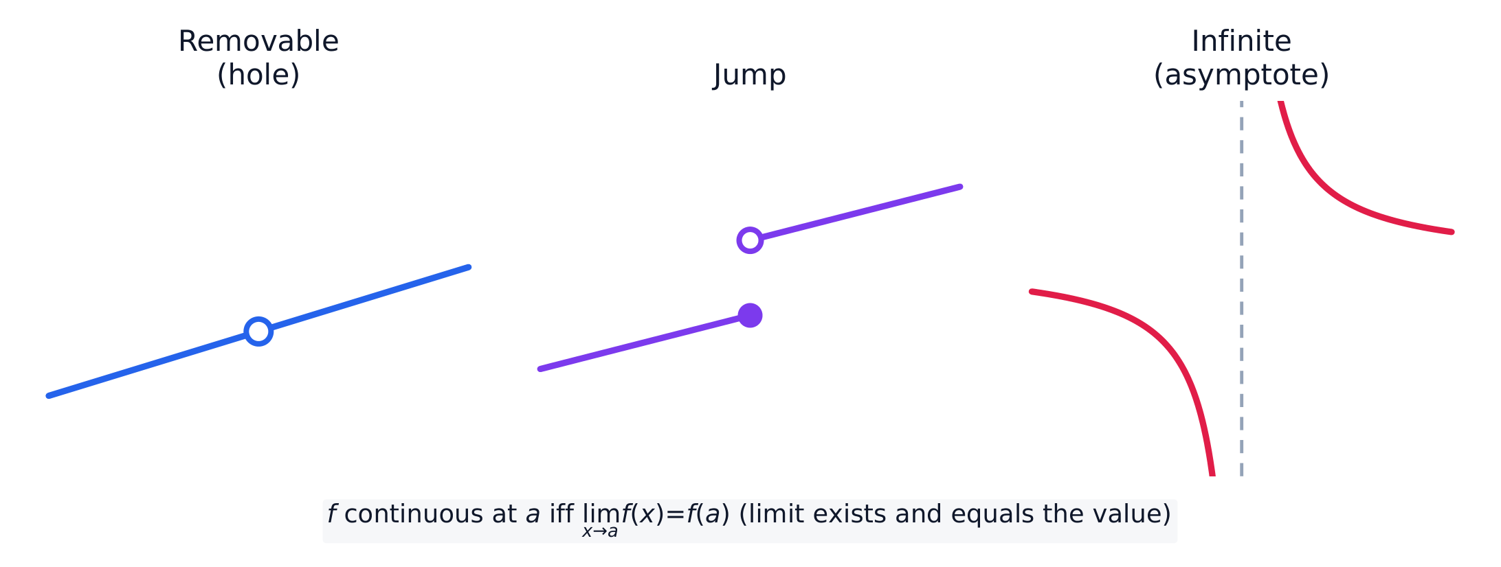
A function is discontinuous 间断 at $c$ when its graph "breaks" there. There are three types:
- Removable discontinuity 可去间断 – a single hole. The two-sided limit exists, but the point is missing or misplaced.
- Jump discontinuity 跳跃间断 – the two one-sided limits exist but disagree, so the curve jumps.
- Infinite discontinuity 无穷间断 – the function blows up to $\pm\infty$ at a vertical asymptote 垂直渐近线.
Worked comparison: classify and justify a repair
At 2, $A(x)=(x^2-4)/(x-2)$ simplifies to $x+2$ for $x\ne 2$. Its limit is 4; define $A(2)=4$ to remove the hole. In contrast, $B(x)=1$ for $x<2$ and 3 for $x\ge 2$ has unequal finite one-sided limits 1 and 3. Changing $B(2)$ cannot remove its jump. For $C(x)=1/(x-2)$, the left side tends to $-\infty$ and the right to $+\infty$: an infinite discontinuity, with no finite limit to use as a repair.
Vocabulary
Train
| English |
|---|
| discontinuous/dɪskənˈtɪnjuːəs/ |
| Removable discontinuity/rɪˈmuːvəbl dɪskɒntɪˈnjuːɪti/ |
| Jump discontinuity/dʒʌmp dɪskɒntɪˈnjuːɪti/ |
| Infinite discontinuity/ˈɪnfɪnət dɪskɒntɪˈnjuːɪti/ |
| vertical asymptote/ˈvɜːtɪkl ˈæsɪmptəʊt/ |
1.11
Defining Continuity at a Point
Syllabus
| Enduring Understanding | Learning Objective | Essential Knowledge |
|---|---|---|
LIM-2 | LIM-2.A |
|
Source: College Board AP Course and Exam Description
Continuity is defined by a three-part test. A function $f$ is continuous 连续 at $x=c$ exactly when all three hold:
$$\boxed{\;f(c)\text{ exists}\quad\text{and}\quad \lim_{x\to c} f(x)\text{ exists}\quad\text{and}\quad \lim_{x\to c} f(x) = f(c)\;}$$
In words: the point is there, the limit is there, and the two agree. If any one fails, $f$ is discontinuous at $c$. This test is the backbone of nearly every continuity question, so learn it as a checklist.
Vocabulary
Train
| English |
|---|
| continuous/kənˈtɪnjuːəs/ |
1.12
Confirming Continuity over an Interval
Syllabus
| Enduring Understanding | Learning Objective | Essential Knowledge |
|---|---|---|
LIM-2 | LIM-2.B |
|
Source: College Board AP Course and Exam Description
A function is continuous on an interval 在区间上连续 if it is continuous at every point of that interval. You rarely check point by point, because whole families are continuous on their domains:
Polynomial, rational, power, exponential 指数, logarithmic 对数, and trigonometric 三角 functions are continuous at every point of their domains.
So a rational function is continuous everywhere except where its denominator is zero; $\ln x$ is continuous for $x>0$; and so on. Knowing this lets you declare continuity quickly and correctly.
Vocabulary
Train
| English |
|---|
| continuous on an interval/kənˈtɪnjuːəs ɒn ən ˈɪntəvl/ |
| exponential/ˌekspəˈnenʃl/ |
| logarithmic/ˌlɒɡəˈrɪθmɪk/ |
| trigonometric/ˌtrɪɡənəʊˈmetrɪk/ |
1.13
Removing Discontinuities
Syllabus
| Enduring Understanding | Learning Objective | Essential Knowledge |
|---|---|---|
LIM-2 | LIM-2.C |
|
Source: College Board AP Course and Exam Description
If the limit exists at a hole, the discontinuity is removable: redefine the function at that one point to equal the limit, and the graph is repaired. Formally, set the missing value to $\displaystyle \lim_{x\to c} f(x)$.
For a piecewise-defined function 分段函数, continuity at a boundary $x=c$ needs the two pieces to meet: the left piece's value, the right piece's value, and $f(c)$ must all be equal. This is a common exam setup – you solve for a parameter 参数 (an unknown constant) that makes the pieces match:
$$\lim_{x\to c^-} f(x) = \lim_{x\to c^+} f(x) = f(c).$$
Vocabulary
Train
| English |
|---|
| piecewise-defined function/ˈpiːswaɪz dɪˈfaɪnd ˈfʌŋkʃn/ |
| parameter/pəˈræmɪtə/ |
1.14
Connecting Infinite Limits and Vertical Asymptotes
Syllabus
| Enduring Understanding | Learning Objective | Essential Knowledge |
|---|---|---|
LIM-2 | LIM-2.D |
|
Source: College Board AP Course and Exam Description
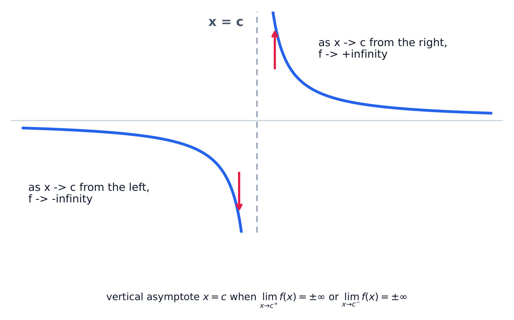
The idea of a limit extends to infinite limits 无穷极限. When a function grows without bound near $x=c$, we write $\lim_{x\to c} f(x) = \pm\infty$. This describes a vertical asymptote at $x=c$: the graph hugs the vertical line $x=c$ and shoots off toward $\pm\infty$.
This happens where a non-zero number is divided by something approaching $0$, such as at a zero of a denominator that does not cancel. Always check each side separately – the two sides can shoot opposite ways (one to $+\infty$, one to $-\infty$).
Explore
Explore infinite limits and vertical asymptotes
y = a/(x − b) + c
With $y=\dfrac{a}{x-b}+c$, watch the curve blow up to $\pm\infty$ near $x=b$. The vertical asymptote is the line $x=b$ where the infinite limit lives — the two sides can shoot opposite ways.
Vocabulary
Train
| English |
|---|
| infinite limits/ˈɪnfɪnət ˈlɪmɪts/ |
1.15
Connecting Limits at Infinity and Horizontal Asymptotes
Syllabus
| Enduring Understanding | Learning Objective | Essential Knowledge |
|---|---|---|
LIM-2 | LIM-2.D |
|
Source: College Board AP Course and Exam Description
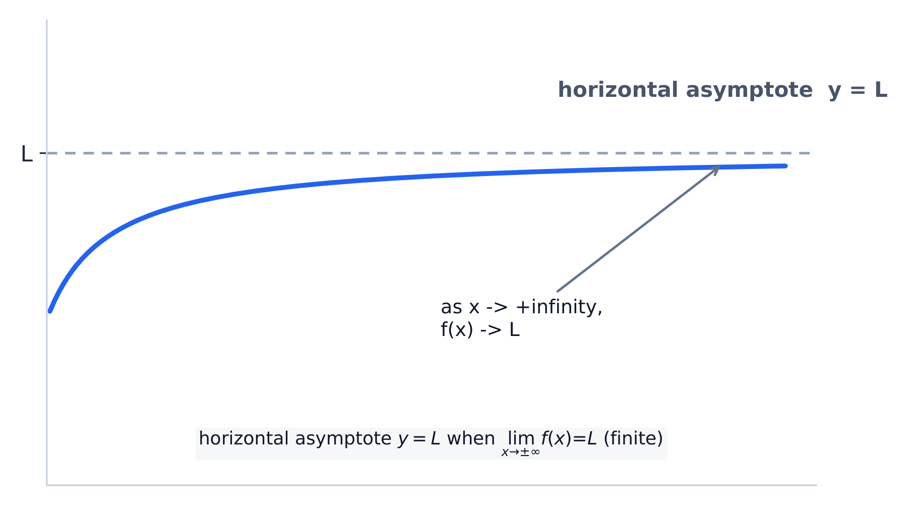
We can also let the input grow: limits at infinity 无穷远处的极限 describe the end behavior 末端行为 of a function as $x\to\pm\infty$. If the outputs settle toward a finite value $L$, then $y=L$ is a horizontal asymptote 水平渐近线.
For a rational function, compare the degrees 次数 of the top and bottom:
- top degree < bottom degree $\Rightarrow$ limit is $0$ (asymptote $y=0$);
- top degree = bottom degree $\Rightarrow$ limit is the ratio of the leading coefficients 首项系数之比;
- top degree > bottom degree $\Rightarrow$ the function is unbounded (no horizontal asymptote).
More generally, we compare the relative magnitudes 相对大小 (relative growth rates) of functions: far out, an exponential beats any polynomial, and a polynomial beats any logarithm. On the exam, "as $t\to\infty$, which quantity is larger/where does the rate settle?" is answered with a limit at infinity.
Explore
Explore limits at infinity and horizontal asymptotes
y = a/(x − b) + c
Follow the curve far out to the right and left. As $x\to\pm\infty$ the outputs settle toward $c$, so $y=c$ is a horizontal asymptote — the finite value of the limit at infinity.
Vocabulary
Train
| English |
|---|
| limits at infinity/ˈlɪmɪts æt ɪnˈfɪnɪti/ |
| end behavior/end bɪˈheɪvjə/ |
| horizontal asymptote/ˌhɒrɪˈzɒntl ˈæsɪmptəʊt/ |
| degrees/dɪˈɡriːz/ |
| ratio of the leading coefficients/ˈreɪʃɪəʊ ɒvðə ˈliːdɪŋ ˌkəʊɪˈfɪʃənts/ |
| relative magnitudes/ˈrelətɪv ˈmæɡnɪtjuːdz/ |
1.16
Working with the Intermediate Value Theorem (IVT)
Syllabus
| Enduring Understanding | Learning Objective | Essential Knowledge |
|---|---|---|
FUN-1 | FUN-1.A |
|
Source: College Board AP Course and Exam Description
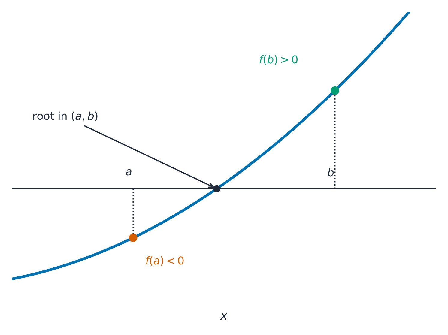
The Intermediate Value Theorem 介值定理 is an existence theorem 存在性定理 – it guarantees a value exists without telling you where:
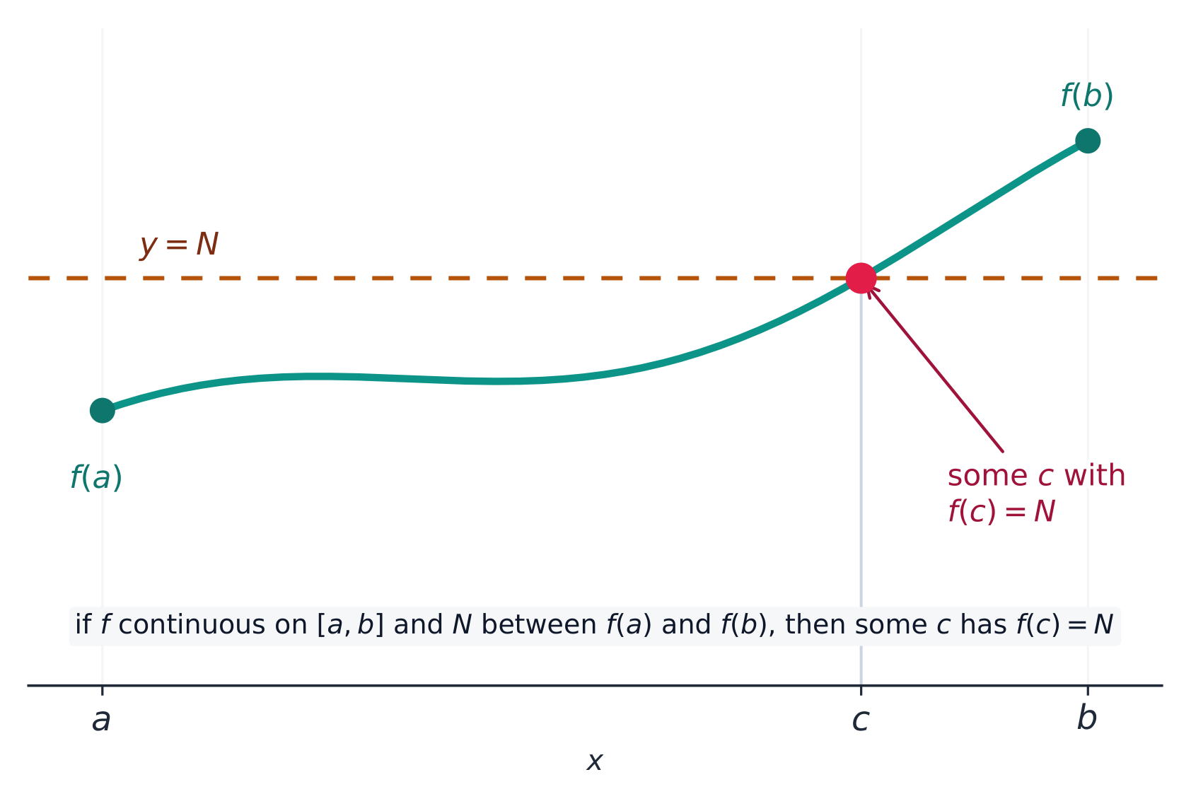
If $f$ is continuous on the closed interval $[a,b]$, and $d$ is any number between $f(a)$ and $f(b)$, then there is at least one number $c$ in $(a,b)$ with $f(c)=d$.
An unbroken curve cannot skip a height between its endpoints – it must pass through every one.
Exam skill – how to justify with the IVT. These questions appear almost every year (for example, "Must there be a value $c$ with $R(c)=155$?" or "Is there a time when $r'(t)=-6$?"). A full-credit justification has three moves:
- State continuity. Say the function is continuous on $[a,b]$ (often because it is differentiable, or given continuous).
- Show $d$ is trapped. Compute the two endpoint values and show the target $d$ lies between them, e.g. $f(a) < d < f(b)$.
- Conclude by name. "By the Intermediate Value Theorem, there is a $c$ in $(a,b)$ with $f(c)=d$."
Skipping the continuity statement, or not showing $d$ is between the endpoints, loses the point – the theorem requires both conditions.
Worked example. Evaluate $\lim_{x\to 3}\dfrac{x^2-9}{x-3}$. Direct substitution gives $\tfrac{0}{0}$ (indeterminate), so factor: $\dfrac{(x-3)(x+3)}{x-3}=x+3$ for $x\ne 3$. Then $\lim_{x\to 3}(x+3)=6$. The graph has a removable discontinuity (a hole) at $x=3$ — the limit exists even though the function is undefined there.
Explore
Why a continuous curve can't skip a value
y = ax³ + bx² + cx + d
The Intermediate Value Theorem: a function continuous on $[a,b]$ takes every $y$ between $f(a)$ and $f(b)$ at some point inside. An unbroken curve cannot leap over a height — it must pass through it.
Vocabulary
Train
| English |
|---|
| Intermediate Value Theorem/ˌɪntəˈmiːdɪət ˈvæljuː ˈθɪərəm/ |
| existence theorem/eɡˈzɪstəns ˈθɪərəm/ |
1.16
Exam tips
- A limit describes what $f(x)$ approaches, which need not equal $f(a)$ — the two-sided limit exists only if both sides agree.
- Try direct substitution first; for a $\tfrac00$ form, factor and cancel or rationalise before substituting.
- A function is continuous at $a$ when the limit exists, $f(a)$ is defined, and they are equal.
- Use the Intermediate Value Theorem to guarantee a root: a continuous function that changes sign on $[a,b]$ takes every value between.
- Read horizontal asymptotes from end behaviour (limits at $\pm\infty$) and vertical asymptotes where the denominator (not the numerator) is zero.
Interactive lessons on this topic
Work through it step by step, with instant-check exercises.
- Introducing Calculus: Can Change Occur at an Instant?
- Defining Limits and Using Limit Notation
- Estimating Limit Values from Graphs
- Estimating Limit Values from Tables
- Determining Limits Using Algebraic Properties of Limits
- Determining Limits Using Algebraic Manipulation
- Selecting Procedures for Determining Limits
- Determining Limits Using the Squeeze Theorem
- Connecting Multiple Representations of Limits
- Exploring Types of Discontinuities
- Defining Continuity at a Point
- Confirming Continuity over an Interval
- Removing Discontinuities
- Connecting Infinite Limits and Vertical Asymptotes
- Connecting Limits at Infinity and Horizontal Asymptotes
- Working with the Intermediate Value Theorem (IVT)