This handout covers Topic 1: Pure Mathematics 纯数学 1. It is the algebra 代数 and calculus 微积分 core of the course. Each ## section is one syllabus subtopic.
팁
A-Level Mathematics (9709) is built from components, not taught as one block: Pure 1, 2 and 3, Mechanics, and Probability & Statistics 1 and 2. Which you sit depends on your school's entry — check that before you plan revision. There is no point grinding Mechanics if you are entered for Statistics.
Pure is the spine. Everything else assumes you can differentiate, integrate and handle algebra without thinking. Weakness there shows up as lost marks in Mechanics and Statistics, not in Pure.
Method marks are generous, and they are awarded for what you wrote down. Showing every line is the highest-return habit in this subject.
-
1
순수 수학 1
수업 보기1.1
Quadratics

Syllabus
Candidates should be able to: Notes and examples carry out the process of completing the square for a quadratic polynomial $ax^2 + bx + c$ and use a completed square form e.g. to locate the vertex of the graph of $y = ax^2 + bx + c$ or to sketch the graph find the discriminant of a quadratic polynomial $ax^2 + bx + c$ and use the discriminant e.g. to determine the number of real roots of the equation $ax^2 + bx + c = 0$. Knowledge of the term ‘repeated root’ is included. solve quadratic equations, and quadratic inequalities, in one unknown By factorising, completing the square and using the formula. solve by substitution a pair of simultaneous equations of which one is linear and one is quadratic e.g. $x + y + 1 = 0$ and $x^2 + y^2 = 25$, $2x + 3y = 7$ and $3x^2 = 4 + 4xy$. recognise and solve equations in $x$ which are quadratic in some function of $x$. e.g. $x^4 - 5x^2 + 4 = 0$, $6x + \sqrt{x} - 1 = 0$, $\tan^2 x = 1 + \tan x$. 출처: Cambridge International syllabus
Completing the square finds the vertex A suspension bridge: the main cable hangs in a parabola. A quadratic 二次式 is an expression of the form $ax^2 + bx + c$, where $a \neq 0$. The letters $a$, $b$, $c$ are the coefficients 系数 (the fixed numbers). Much of this section is about solving the equation $ax^2 + bx + c = 0$.
Completing the square
To complete the square 配方 means to write the quadratic in the form
$$a(x + p)^2 + q.$$This form is useful: it shows the vertex 顶点 (turning point) of the curve at $(-p,\ q)$, and it gives a quick way to solve the equation.Worked example. Write $9x^2 - 36x + 8$ in the form $p(x + q)^2 + r$.
Take the factor $9$ out of the first two terms, then complete the square inside:
$$\begin{aligned} 9x^2 - 36x + 8 &= 9\left(x^2 - 4x\right) + 8 \\ &= 9\left((x - 2)^2 - 4\right) + 8 \\ &= 9(x - 2)^2 - 36 + 8 = 9(x - 2)^2 - 28. \end{aligned}$$So $p = 9$, $q = -2$, $r = -28$.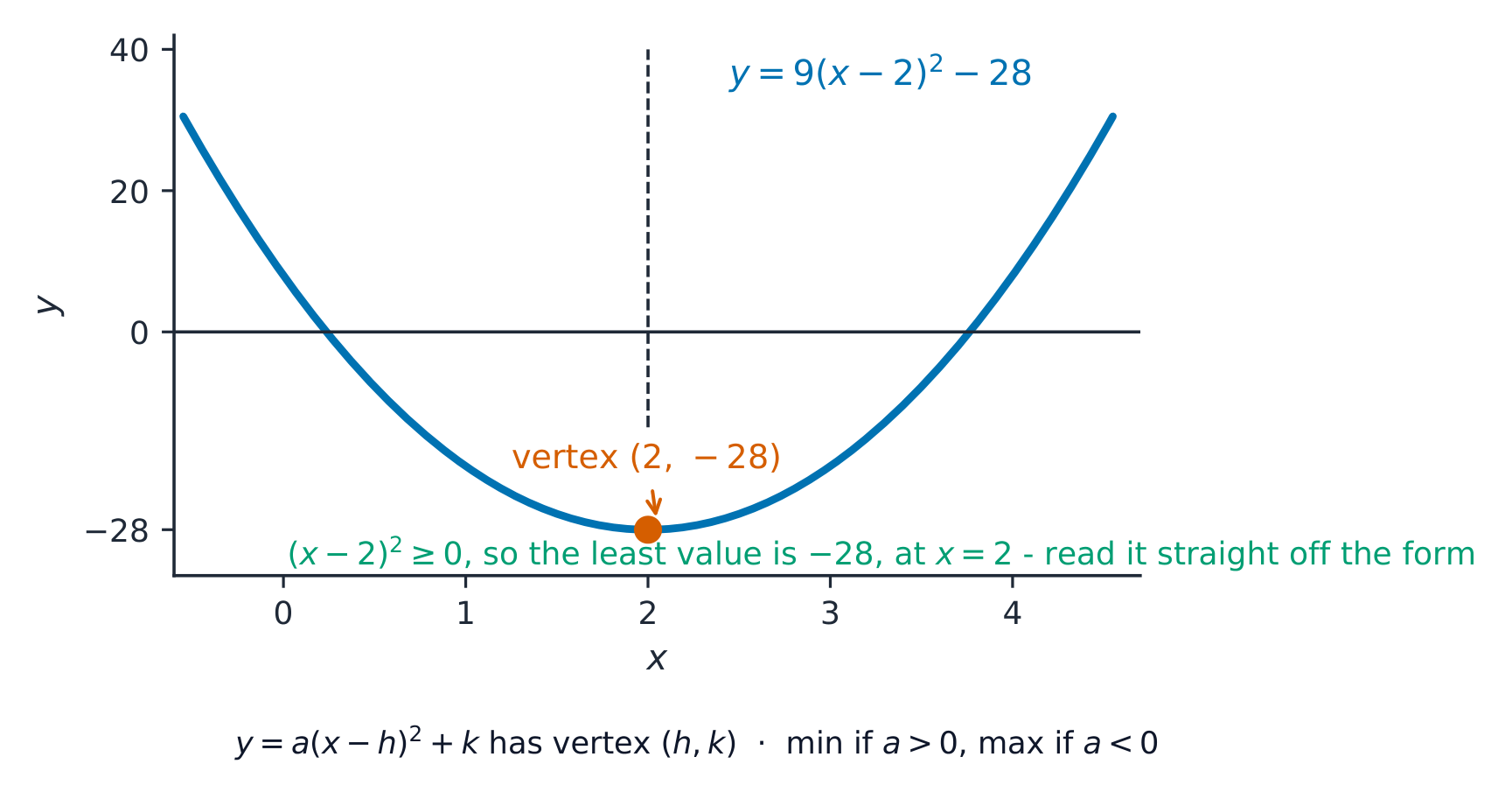
The completed square hands you the vertex: least value -28 at x equals 2 The discriminant
The discriminant 判别式 of $ax^2 + bx + c$ is
$$\Delta = b^2 - 4ac.$$It tells you how many real roots 实根 (real solutions) the equation $ax^2 + bx + c = 0$ has:Discriminant Roots $b^2 - 4ac > 0$ two distinct 相异 real roots $b^2 - 4ac = 0$ one repeated real root $b^2 - 4ac < 0$ no real roots 
The sign of $b^2-4ac$ decides how many times the parabola meets the $x$-axis. Worked example. Find the values of the constant $k$ for which $3kx^2 + (k + 8)x + 3 = 0$ has two distinct real roots.
Here $a = 3k$, $b = k + 8$, $c = 3$. For two distinct real roots you need $b^2 - 4ac > 0$:
$$(k + 8)^2 - 4(3k)(3) > 0 \;\Rightarrow\; k^2 + 16k + 64 - 36k > 0 \;\Rightarrow\; k^2 - 20k + 64 > 0.$$Factorise: $(k - 4)(k - 16) > 0$, so $k < 4$ or $k > 16$. You also need $a \neq 0$, so $k \neq 0$.Quadratic equations and inequalities
To solve a quadratic equation 二次方程, factorise, complete the square, or use the formula
$$x = \frac{-b \pm \sqrt{b^2 - 4ac}}{2a}.$$To solve a quadratic inequality 二次不等式 such as $(k - 4)(k - 16) > 0$, find the two roots, then decide which side of each root makes the statement true. A sketch of the parabola 抛物线 helps: the curve is above the $x$-axis (positive) outside the roots and below it (negative) between them.Simultaneous equations
To solve a pair of simultaneous equations 联立方程 where one is linear and one is quadratic, use substitution 代入: rearrange the linear equation for one letter, then put that into the quadratic. This gives a single quadratic to solve.
Equations that are quadratic in disguise
Some equations are quadratic in some function of $x$. For example $x^4 - 5x^2 + 4 = 0$ is quadratic in $x^2$: let $u = x^2$, solve $u^2 - 5u + 4 = 0$, then go back to $x$. You will use this idea again in trigonometry.
탐색하기이차함수의 형태
y = ax² + bx + c
a, b, c를 드래그하세요. 계수가 변함에 따라 꼭짓점, 대칭축, 그리고 근(root) (x축과 만나는 지점)이 어떻게 이동하는지 확인하세요.
어휘 연습하기English 한국어 Pure Mathematics/pjʊə ˌmæθɪˈmætɪks/ 순수 수학(Pure Mathematics) quadratic/kwɒˈdrætɪk/ 이차 complete the square/kəmˈpliːt ðə skweə/ 제곱완성(complete the square) vertex/ˈvɜːteks/ 정점 discriminant/dɪˈskrɪmɪnənt/ 판별식 real roots/rɪəl ruːts/ 실근(real roots) distinct/dɪˈstɪŋkt/ 서로 다른(distinct) quadratic equation/kwɒˈdrætɪk ɪˈkweɪʒn/ 이차 방정식(quadratic equation) quadratic inequality/kwɒˈdrætɪk ɪniːˈkwɒlɪti/ 이차 부등식(quadratic inequality) simultaneous equations/ˌsɪməlˈteɪnɪəs ɪˈkweɪʒnz/ 연립방정식 substitution/ˌsʌbstɪˈtjuːʃn/ 치환(substitution) coefficient/ˌkəʊɪˈfɪʃənt/ 계수 parabola/pəˈræbələ/ 포물선Unless parabola. 1.2
Functions
Syllabus
지원자는 다음을 할 수 있어야 한다: 참고 사항 및 예시 함수, 정의역, 치역, 일대일 함수, 역함수 및 함수의 합성이라는 용어를 이해한다 주어진 함수의 범위를 식별하고, 두 함수의 합성을 구한다 예: $f : x \mapsto \frac{1}{x}$에 대한 $x \geqslant 1$의 범위 및 $g : x \mapsto x^2 + 1$에 대한 $x \in \mathbb{R}$의 범위. 합성함수 $gf$는 $f$의 범위가 $g$의 정의역에 포함되어야만 구성될 수 있다는 조건 포함. 주어진 함수가 일대일인지 판별하고, 일대일 함수의 역함수를 구한다 (간단한 경우) 예: $h : x \mapsto (2x + 3)^2 - 4$에 대한 $x < -\frac{3}{2}$의 역함수 구하기. 일대일 함수와 그 역함수 사이의 관계를 그래프로 나타낸다 스케치는 반사선 $y = x$를 표시해야 한다. 주어진 $y = f(x)$에 대한 $y = f(x) + a$, $y = f(x + a)$, $y = af(x)$, $y = f(ax)$ 및 이들의 간단한 조합에 의한 그래프의 변환을 이해하고 사용한다 변환을 설명할 때 ‘平移’, ‘반사’, ‘늘림’ 등의 용어를 사용하는 것을 포함한다. questions may involve algebraic or trigonometric functions, or other graphs with given features. 출처: Cambridge International syllabus
Transforming graphs: shift and stretch A function 函数 is a rule that sends each input to exactly one output. Write it as $f(x)$. The composition of functions 复合函数 $fg(x)$ means apply $g$ first, then apply $f$ to the result.
- The domain 定义域 is the set of allowed inputs $x$.
- The range 值域 is the set of outputs the function actually produces.
A function is one-one 一一对应 if different inputs always give different outputs. (No output is repeated.) Only a one-one function has an inverse function 反函数 $f^{-1}$, which reverses the rule.
The composition 复合 of two functions means doing one after the other. $fg(x)$ means "do $g$ first, then $f$": $fg(x) = f(g(x))$. The composite function $fg$ exists only when the range of $g$ lies inside the domain of $f$.
Finding an inverse
To find $f^{-1}$: write $y = f(x)$, make $x$ the subject, then swap letters.
Worked example. The function $f(x) = (x + 3)^2 - 12$ is defined for $x \geqslant 0$. Find $f^{-1}(x)$.
Write $y = (x + 3)^2 - 12$ and solve for $x$:
$$(x + 3)^2 = y + 12 \;\Rightarrow\; x + 3 = \sqrt{y + 12} \;\Rightarrow\; x = \sqrt{y + 12} - 3.$$You take the positive square root because $x \geqslant 0$ means $x + 3 \geqslant 3 > 0$. So$$f^{-1}(x) = \sqrt{x + 12} - 3.$$Graphs of inverses and transformations
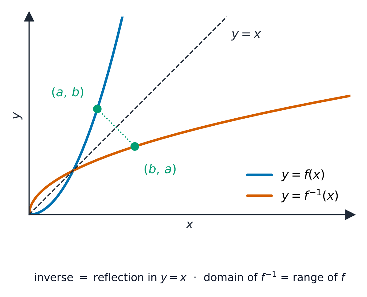
The graph of $y = f^{-1}(x)$ is the reflection 反射 of $y = f(x)$ in the line $y = x$.
Reflecting $y=f(x)$ in the line $y=x$ gives its inverse; a point $(a,b)$ becomes $(b,a)$. You should know these transformations 变换 of $y = f(x)$:
New equation Effect on the graph $y = f(x) + a$ translation 平移 up by $a$ $y = f(x + a)$ translation left by $a$ $y = a\,f(x)$ stretch 伸缩 in the $y$-direction, scale factor $a$ $y = f(ax)$ stretch in the $x$-direction, scale factor $\tfrac{1}{a}$ When two transformations are combined, the order can matter. State each one fully (type, direction, and amount).

Adding to the output or input slides the curve; a multiplier stretches it. 탐색하기함수 탐색하기
y = ax³ + bx² + cx + d
함수는 각 입력을 정확히 하나의 출력로 변환합니다 — 계수를 드래그하여 곡선이 오르내림하는 지점을 관찰하세요.
어휘 연습하기English 한국어 function/ˈfʌŋkʃn/ 함수(function) composition of functions/ˌkɒmpəˈzɪʃn ɒv ˈfʌŋkʃnz/ 함수의 합성(composition of functions) domain/dəˈmeɪn/ 정의역 range/reɪndʒ/ 범위Unless range. one-one/wʌn wʌn/ 일대일 inverse function/ɪnˈvɜːs ˈfʌŋkʃn/ 역함수 composition/ˌkɒmpəˈzɪʃn/ 구도 reflection/rɪˈflekʃn/ 반사각 transformations/trænsfɔːˈmeɪʃnz/ 변환 translation/trænˈsleɪʃn/ 번역 stretch/stretʃ/ 신축Unless stretch in geometry/transformation. 1.3
Coordinate geometry

Syllabus
지원자는 다음을 할 수 있어야 한다: 참고 사항 및 예시 충분한 정보를 주어 직선의 방정식을 구한다 e.g. 두 점 또는 한 점과 기울기를 줄 때. 문제 해결 시 $y = mx + c$, $y - y_1 = m(x - x_1)$, $ax + by + c = 0$ 형태의任何一方를 해석하고 사용한다 거리 계산, 기울기, 중점, 교점 및 평행 및 수직 직선 사이의 기울기 관계 활용을 포함한다. 방정식 $(x - a)^2 + (y - b)^2 = r^2$가 중심 $(a, b)$이고 반지름 $r$인 원임을 이해한다 전개된 형태 $x^2 + y^2 + 2gx + 2fy + c = 0$의 사용을 포함한다. 직선과 원에 관련된 문제를 대수적으로 풀기 원의 기본 기하학적 성질(예: 접선은 반지름에 수직, 반원의 안각, 대칭성) 사용을 포함한다. 암묵적 미분은 포함되지 않는다. 그래프와 그에 대응하는 대수 방정식 간의 관계를 이해하고, 그래프의 교점과 방정식의 해 간의 관계를 사용한다. e.g. 방정식 $k$에 대해 직선 $y = x + k$이 이차 곡선과 교차하거나 접하거나 만나지 않는 값의 범위를 결정할 때. 출처: Cambridge International syllabus
Coordinate geometry 坐标几何 studies lines and circles using their equations.
Straight lines
The gradient 斜率 (steepness) of the line joining $(x_1, y_1)$ and $(x_2, y_2)$ is
$$m = \frac{y_2 - y_1}{x_2 - x_1}.$$You can write the equation of a straight line 直线方程 in any of these forms:$$y = mx + c, \qquad y - y_1 = m(x - x_1), \qquad ax + by + c = 0.$$Two lines are parallel 平行 when their gradients are equal, and perpendicular 垂直 (at right angles) when the product of their gradients is $-1$.Circles
The circle 圆 with centre 圆心 $(a, b)$ and radius 半径 $r$ has equation
$$(x - a)^2 + (y - b)^2 = r^2.$$An expanded form like $x^2 + y^2 - 6x + 10y - 27 = 0$ is the same circle: complete the square in $x$ and in $y$ to find the centre and radius.A tangent 切线 to a circle touches it at one point and is perpendicular to the radius at that point. This right-angle fact solves most circle problems.
A tangent touches the circle once and meets the radius at a right angle. Worked example. The points $P(1, 1)$ and $Q(7, 11)$ are the ends of a diameter 直径 of a circle. Find the equation of the circle.
The centre is the midpoint of $PQ$:
$$\left(\frac{1 + 7}{2},\ \frac{1 + 11}{2}\right) = (4, 6).$$The radius is half the length of $PQ$:$$r = \tfrac12\sqrt{(7 - 1)^2 + (11 - 1)^2} = \tfrac12\sqrt{36 + 100} = \tfrac12\sqrt{136} = \sqrt{34}.$$So the circle is $(x - 4)^2 + (y - 6)^2 = 34$.탐색하기직선
y = ax + b
기울기 a가 선을 기울이고, 절편 b가 선을 위아래로 이동시킵니다.
어휘 연습하기English 한국어 Coordinate geometry/kəʊˈɔːdɪnət dʒiˈɒmətri/ 좌표 기하학 gradient/ˈɡreɪdɪənt/ 기울기 equation of a straight line/ɪˈkweɪʒn əvə streɪt laɪn/ 직선의 방정식(equation of a straight line) parallel/ˈpærəlel/ 평행 perpendicular/ˌpɜːpənˈdɪkjʊlə/ 수직Unless perpendicular lines/planes. circle/ˈsɜːkl/ 원 centre/ˈsentə/ 무게 중심 radius/ˈreɪdɪəs/ 반경 tangent/ˈtændʒənt/ 접선 diameter/daɪˈæmɪtə/ 직경 1.4
Circular measure

Syllabus
지원자는 다음을 할 수 있어야 한다: 참고 사항 및 예시 라디안의 정의를 이해하고 라디안과 도 사이의 관계를 사용한다 원의 호 길이와 부채꼴 면적에 관한 문제 해결 시 $s = r\theta$ 및 $A = \frac{1}{2}r^2\theta$ 공식을 사용한다. 삼각형 내 길이 및 각도 계산, 삼각형 면적 계산을 포함한다. 출처: Cambridge International syllabus
What is a radian? Radians
A radian 弧度 is another way to measure angles. One radian is the angle at the centre of a circle that cuts off an arc 弧 equal in length to the radius. The link between radians and degrees 度 is
$$\pi \text{ radians} = 180^\circ.$$So to change degrees to radians, multiply by $\dfrac{\pi}{180}$; to change radians to degrees, multiply by $\dfrac{180}{\pi}$.One radian: the angle whose arc equals the radius Arc length and sector area
For a sector 扇形 with radius $r$ and angle $\theta$ in radians:
$$\text{arc length} = s = r\theta, \qquad \text{sector area} = A = \tfrac12 r^2 \theta.$$A chord 弦 cuts the sector into a triangle and a segment 弓形. The segment area is the sector minus the triangle:$$\text{segment} = \tfrac12 r^2 \theta - \tfrac12 r^2 \sin\theta = \tfrac12 r^2(\theta - \sin\theta).$$
The shaded segment is the part of the sector between the chord and the arc. Worked example. A sector has centre $O$ and the angle at $O$ is $\tfrac{2}{3}\pi$ radians. Show that the segment cut off by the chord has area about $0.614 r^2$.
$$\text{segment} = \tfrac12 r^2\left(\tfrac{2}{3}\pi - \sin\tfrac{2}{3}\pi\right) = \tfrac12 r^2(2.0944 - 0.8660) = \tfrac12 r^2(1.2284) \approx 0.614 r^2.$$탐색하기라디안, 호(arc)와 부채 sector
각도(라디안 단위)와 반지름을 변경하세요. 호의 길이 $s = r\theta$와 부채의 면적 $\tfrac12 r^2\theta$가 업데이트되는 것을 확인하세요.
어휘 연습하기English 한국어 radian/ˈreɪdɪən/ 라디안 arc/ɑːk/ 호 degrees/dɪˈɡriːz/ 도 sector/ˈsektə/ 세クター chord/kɔːd/ 현 segment/ˈseɡmənt/ 세그먼트(시장 구분) 1.5
Trigonometry

Syllabus
지원자는 다음을 할 수 있어야 한다: 참고 사항 및 예시 사인, 코사인, 탄젠트 함수의 그래프를 스케치하고 활용한다 (임의의 크기의 각도에 대해, 도 또는 라디안을 사용하여) 예: $y = 3 \sin x$, $y = 1 - \cos 2x$, $y = \tan(x + \frac{1}{4}\pi)$ 등. $30^\circ$, $45^\circ$, $60^\circ$ 및 관련 각도의 사인, 코사인, 탄젠트의 정확한 값을 사용한다 예: $\cos 150^\circ = -\frac{1}{2}\sqrt{3}$, $\sin \frac{3}{4}\pi = \frac{1}{\sqrt{2}}$ 등. 역삼각함수 관계의 주값을 나타내는 기호 $\sin^{-1} x$, $\cos^{-1} x$, $\tan^{-1} x$를 사용한다 이 함수들에 대한 전문 지식은 필요하지 않으나, 역함수의 예로서 이해하고 있어야 한다. 항등식 $\frac{\sin \theta}{\cos \theta} \equiv \tan \theta$과 $\sin^2 \theta + \cos^2 \theta \equiv 1$를 사용한다 예: 항등식 증명, 식 정리, 방정식 풀이에 활용. 주어진 구간 내에 있는 간단한 삼각방정식의 모든 해를 구한다 (해의 일반형은 포함되지 않음). 예: $3 \sin 2x + 1 = 0$를 $-\pi < x < \pi$에 대해, $3 \sin^2 \theta - 5 \cos \theta - 1 = 0$를 $0^\circ \leqslant \theta \leqslant 360^\circ$에 대해 푸는 것 등. 출처: Cambridge International syllabus
Amplitude, period and midline of a sine curve The unit circle draws the sine curve A Ferris wheel: a point on the rim rises and falls like a sine curve. Graphs and exact values
You must know the shape of the graphs of the sine 正弦, cosine 余弦 and tangent function 正切 (written $\sin$, $\cos$, $\tan$). The sine and cosine graphs wave between $-1$ and $1$ and repeat every $360^\circ$ ($2\pi$). Learn these exact values:
$\theta$ $30^\circ$ $45^\circ$ $60^\circ$ $\sin\theta$ $\tfrac12$ $\tfrac{1}{\sqrt2}$ $\tfrac{\sqrt3}{2}$ $\cos\theta$ $\tfrac{\sqrt3}{2}$ $\tfrac{1}{\sqrt2}$ $\tfrac12$ $\tan\theta$ $\tfrac{1}{\sqrt3}$ $1$ $\sqrt3$ 
Over one turn $\sin$ and $\cos$ stay between $-1$ and $1$; $\tan$ shoots off at $90^\circ$ and $270^\circ$. The notations $\sin^{-1}x$, $\cos^{-1}x$, $\tan^{-1}x$ mean the inverse angle (the principal value 主值).
Identities
An identity 恒等式 is true for every value of the angle. The two you must know are
$$\tan\theta \equiv \frac{\sin\theta}{\cos\theta}, \qquad \sin^2\theta + \cos^2\theta \equiv 1.$$Use them to rewrite an equation so it contains only one trig function.Solving trigonometric equations
To solve a trigonometric equation 三角方程, first reduce it to one function, then find every solution in the given interval.
Worked example. Solve $6\sin\theta = 1 + \dfrac{2}{\sin\theta}$ for $-180^\circ < \theta < 180^\circ$.
Multiply through by $\sin\theta$ to clear the fraction. This makes a quadratic in $\sin\theta$:
$$6\sin^2\theta - \sin\theta - 2 = 0 \;\Rightarrow\; (3\sin\theta - 2)(2\sin\theta + 1) = 0.$$So $\sin\theta = \tfrac23$ or $\sin\theta = -\tfrac12$.- $\sin\theta = \tfrac23$: $\theta = 41.8^\circ$ or $\theta = 180^\circ - 41.8^\circ = 138.2^\circ$.
- $\sin\theta = -\tfrac12$: $\theta = -30^\circ$ or $\theta = -150^\circ$.
The four solutions are $\theta = -150^\circ,\ -30^\circ,\ 41.8^\circ,\ 138.2^\circ$.
탐색하기사인 & 코사인 그래프
y = a·sin(bx + c) + d의 진폭, 주기 및 변위를 드래그하여 기본 파동 대비 곡선이 어떻게 변하는지 관찰하세요.
탐색하기단위 원 위의 사인과 코사인
각도를 단위 원 주위로 드래그하세요. 높이가 $\sin\theta$, 가로 거리가 $\cos\theta$입니다 — 이것이 그래프의 기원입니다.
어휘 연습하기English 한국어 sine/saɪn/ 사인 cosine/ˈkəʊsaɪn/ 코사인 tangent function/ˈtændʒənt ˈfʌŋkʃn/ 탄젠트 함수(tangent function) principal value/ˈprɪnsɪpl ˈvæljuː/ 주 값(principal value) identity/aɪˈdentɪti/ 정체성 trigonometric equation/ˌtrɪɡənəʊˈmetrɪk ɪˈkweɪʒn/ 삼각 방정식(trigonometric equation) 1.6
Series

Syllabus
지원자는 다음을 할 수 있어야 한다: 참고 사항 및 예시 $(a + b)^n$의 전개식을 사용하여, $n$은 양의 정수이다. $\begin{pmatrix} n \\ r \end{pmatrix}$ 및 $n!$의 표기법을 포함한다. 최대항과 계수의 성질에 대한 지식이 필요하지는 않다. 산술급수와 기하급수를 인식한다 산술급수 또는 기하급수 관련 문제 해결을 위해 $n$항의 공식과 전 $n$항의 합 공식을 사용한다 숫자 $a$, $b$, $c$가 $2b = a + c$(또는 동등 조건)일 때 '산술급수'에 있으며, $b^2 = ac$(또는 동등 조건)일 때 '기하급수'에 있다는 지식을 포함한다.问题是涉及多个级数일 수 있다. 기하급수의 수렴 조건과 수렴하는 기하급수의 무한합 공식을 사용한다. 출처: Cambridge International syllabus
Pascal's triangle gives the coefficients Sum to infinity fills the square The binomial expansion
For a positive integer $n$, the binomial expansion 二项展开式 is
$$(a + b)^n = a^n + \binom{n}{1}a^{n-1}b + \binom{n}{2}a^{n-2}b^2 + \cdots + b^n,$$where $\binom{n}{r} = \dfrac{n!}{r!\,(n - r)!}$ is a binomial coefficient 二项式系数.Worked example. Find the first three terms, in ascending powers of $x$, of $(2 - px)^5$.
$$(2 - px)^5 = 2^5 + \binom{5}{1}2^4(-px) + \binom{5}{2}2^3(-px)^2 + \cdots = 32 - 80px + 80p^2x^2 + \cdots$$Arithmetic and geometric progressions
A progression 数列 (sequence) is a list of terms following a rule.
- An arithmetic progression 等差数列 (AP) adds a fixed common difference 公差 $d$ each step. The $n$th term 项 is $u_n = a + (n - 1)d$, and the sum of the first $n$ terms is $S_n = \tfrac{n}{2}\big(2a + (n - 1)d\big)$.
- A geometric progression 等比数列 (GP) multiplies by a fixed common ratio 公比 $r$ each step. The $n$th term is $u_n = ar^{\,n-1}$, and $S_n = \dfrac{a(1 - r^n)}{1 - r}$.
An AP climbs in equal steps; a GP's steps grow by the same ratio A GP is convergent — it converges 收敛 (settles to a limit) — when $|r| < 1$. Then it has a sum to infinity 无穷和
$$S_\infty = \frac{a}{1 - r}.$$Worked example. The third term of a GP is $18$ and the sum of the first three terms is $26$. The common ratio is negative. Find the sum to infinity.
From $ar^2 = 18$ you get $a = \dfrac{18}{r^2}$. Put this into $a(1 + r + r^2) = 26$:
$$18(1 + r + r^2) = 26r^2 \;\Rightarrow\; 8r^2 - 18r - 18 = 0 \;\Rightarrow\; (4r + 3)(r - 3) = 0.$$The ratio is negative, so $r = -\tfrac34$ and $a = \dfrac{18}{(3/4)^2} = 32$. Then$$S_\infty = \frac{32}{1 - (-\tfrac34)} = \frac{32}{\tfrac74} = \frac{128}{7}.$$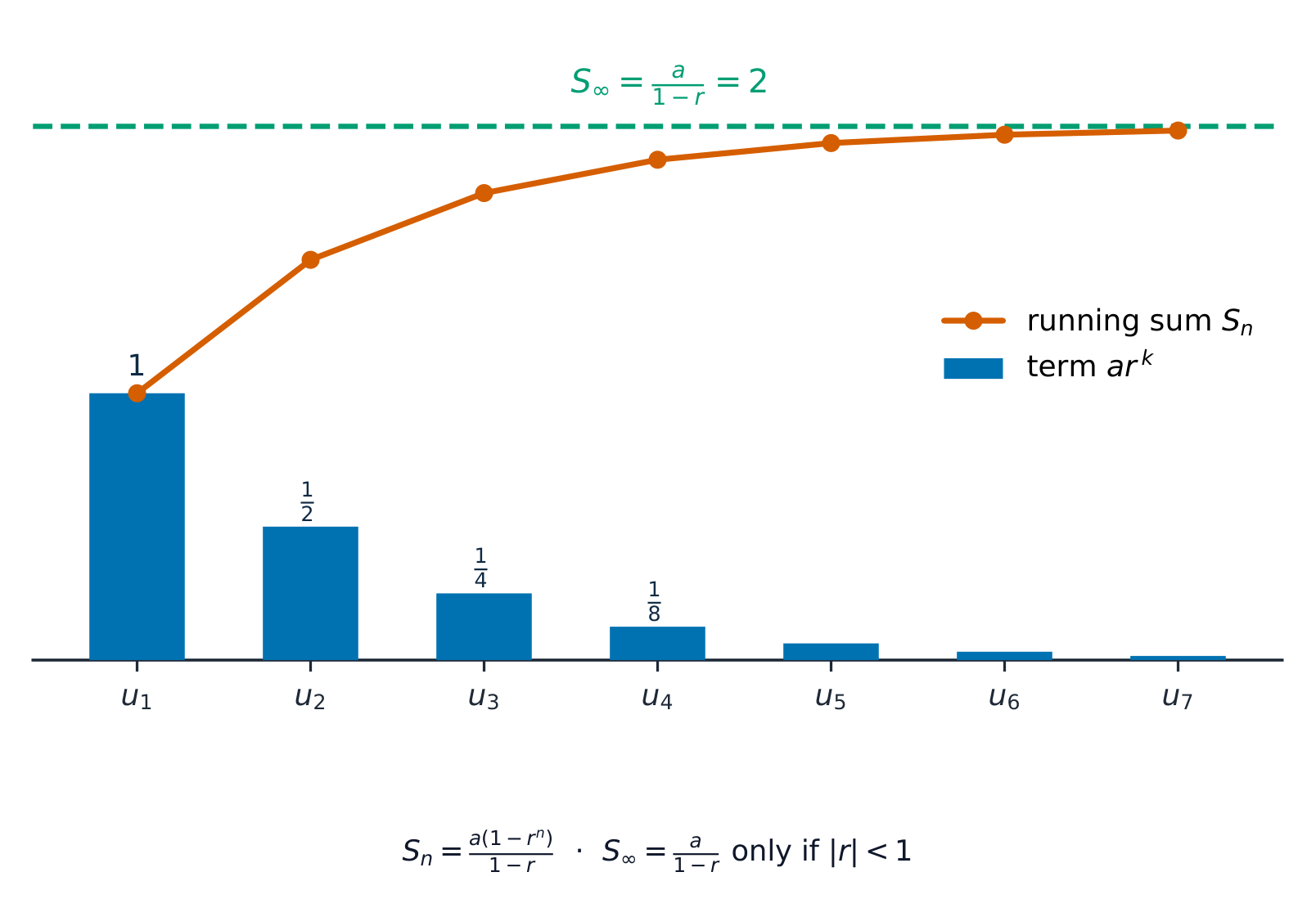
Convergent GP: bars shrink toward zero while the running sum approaches S infinity = a/(1-r) 탐색하기등차수열과 등비수열
등차수열(d를 더함)과 등비수열(r을 곱함)을 전환하며 항들과 합계가 어떻게 쌓이는지 확인하세요.
어휘 연습하기English 한국어 binomial expansion/baɪˈnəʊmɪəl ekˈspænʃn/ 이항 전개 binomial coefficient/baɪˈnəʊmɪəl ˌkəʊɪˈfɪʃənt/ 이항 계수 progression/prəˈɡreʃn/ 수열(progression) arithmetic progression/əˈrɪθmətɪk prəˈɡreʃn/ 등차수열 common difference/ˈkɒmən ˈdɪfrəns/ common difference(등차) term/tɜːm/ 항 geometric progression/ˌdʒiːəʊˈmetrɪk prəˈɡreʃn/ 등비수열 common ratio/ˈkɒmən ˈreɪʃɪəʊ/ common ratio(등비) converges/kənˈvɜːdʒɪz/ 수렴함 sum to infinity/sʌm tʊ ɪnˈfɪnɪti/ 무한 급수의 합 1.7
Differentiation
Syllabus
Candidates should be able to: Notes and examples understand the gradient of a curve at a point as the limit of the gradients of a suitable sequence of chords, and use the notations $f'(x)$, $f''(x)$, $\frac{\text{d}y}{\text{d}x}$, and $\frac{\text{d}^2y}{\text{d}x^2}$ for first and second derivatives Only an informal understanding of the idea of a limit is expected. e.g. includes consideration of the gradient of the chord joining the points with $x$ coordinates $2$ and $(2 + h)$ on the curve $y = x^3$. Formal use of the general method of differentiation from first principles is not required. use the derivative of $x^n$ (for any rational $n$), together with constant multiples, sums and differences of functions, and of composite functions using the chain rule e.g. find $\frac{\text{d}y}{\text{d}x}$, given $y = \sqrt{2x^3 + 5}$. apply differentiation to gradients, tangents and normals, increasing and decreasing functions and rates of change Including connected rates of change, e.g. given the rate of increase of the radius of a circle, find the rate of increase of the area for a specific value of one of the variables. locate stationary points and determine their nature, and use information about stationary points in sketching graphs. Including use of the second derivative for identifying maxima and minima; alternatives may be used in questions where no method is specified. Knowledge of points of inflexion is not included. 출처: Cambridge International syllabus
Differentiation from first principles Differentiation 微分 finds the gradient of a curve 曲线斜率 at each point. The gradient is the limit 极限 of the gradients of shorter and shorter chords, called the derivative 导数.
The rules
Write the derivative as $f'(x)$ or $\dfrac{dy}{dx}$. The basic rule is
$$\frac{d}{dx}\left(x^n\right) = n x^{n-1} \quad \text{for any rational } n.$$Differentiate sums term by term, and use the chain rule 链式法则 for a function inside a function:$$\frac{d}{dx}\,f(g(x)) = f'(g(x)) \cdot g'(x).$$Differentiating again gives the second derivative 二阶导数 $f''(x)$ or $\dfrac{d^2y}{dx^2}$.Using the derivative
- Tangent and normal. The gradient of the curve at a point is the gradient of the tangent there. The normal 法线 is perpendicular to the tangent, so its gradient is $-\dfrac{1}{\text{(tangent gradient)}}$.
- Increasing or decreasing. The function is an increasing function 增函数 where $\dfrac{dy}{dx} > 0$, and a decreasing function 减函数 where $\dfrac{dy}{dx} < 0$.
- Rate of change. A derivative is a rate of change 变化率. Linked rates use the chain rule, e.g. $\dfrac{dy}{dt} = \dfrac{dy}{dx}\cdot\dfrac{dx}{dt}$.
Stationary points
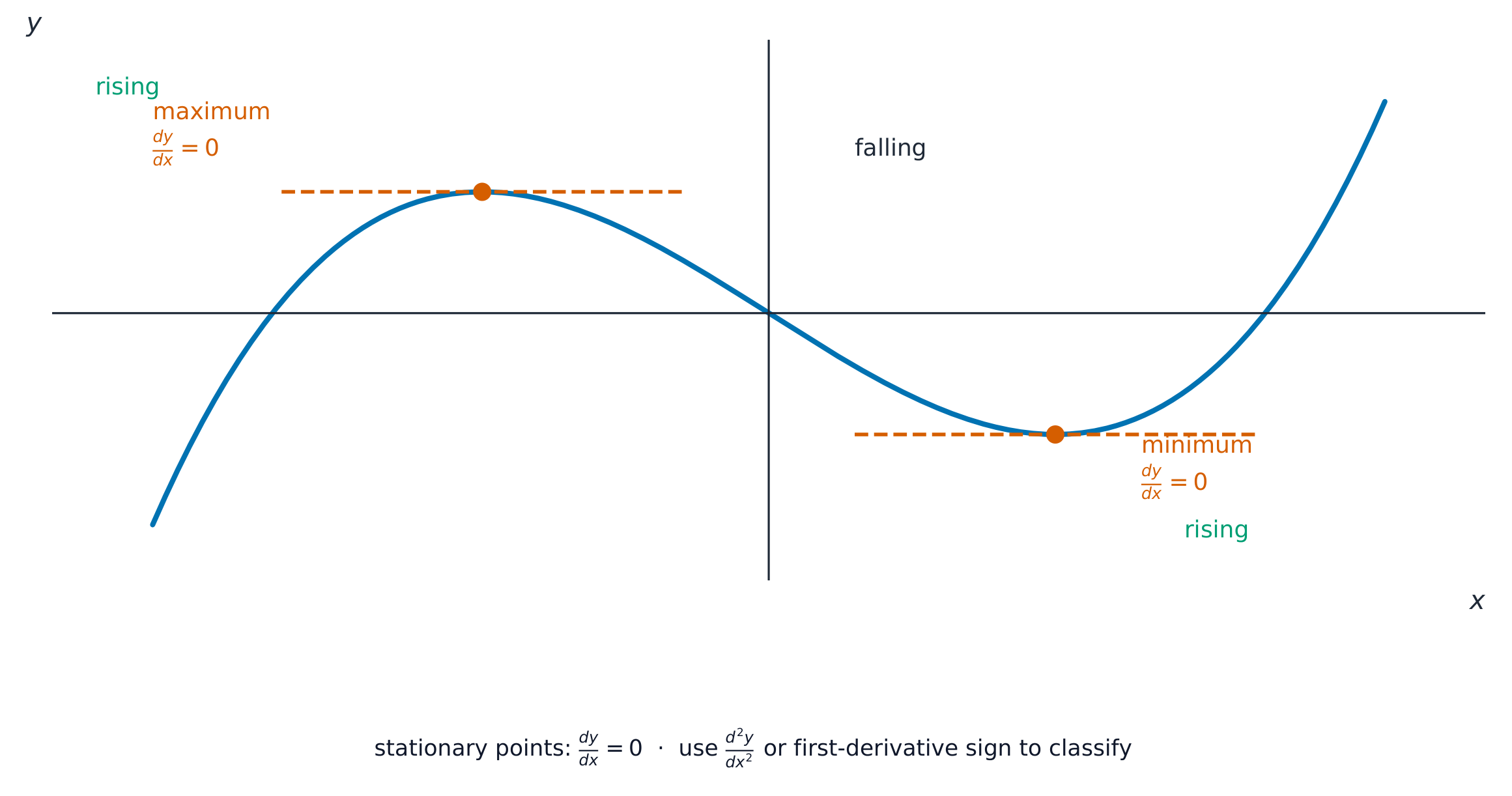
A stationary point 驻点 is where $\dfrac{dy}{dx} = 0$. Test its nature with the second derivative: $f''(x) > 0$ gives a minimum point 极小值点, and $f''(x) < 0$ gives a maximum point 极大值点. When $f''(x) = 0$ the test is inconclusive: the point may be a point of inflexion 拐点, where the curve changes concavity (the way it bends) – check the sign of $\dfrac{dy}{dx}$ just before and after to decide.
At a maximum or a minimum the tangent is flat, so $\frac{dy}{dx}=0$. Worked example. The curve $y = 4x^{1/2} - x$ has a maximum point at $x = a$. Find $a$.
$$\frac{dy}{dx} = 2x^{-1/2} - 1 = 0 \;\Rightarrow\; \frac{2}{\sqrt{x}} = 1 \;\Rightarrow\; \sqrt{x} = 2 \;\Rightarrow\; x = 4.$$So $a = 4$.탐색하기한 점에서의 기울기
y = ax³ + bx² + cx + d
점을 곡선 위에滑动(sliding)하세요. 접선(tangent) 은 해당 지점의 기울기 $\frac{dy}{dx}$를 나타내며, 곡선이 더 굽은 곳에서 더 가파릅니다.
어휘 연습하기English 한국어 Differentiation/ˌdɪfəˌrenʃɪˈeɪʃn/ 미분 gradient of a curve/ˈɡreɪdɪənt əvə kɜːv/ 곡선의 기울기(gradient of a curve) limit/ˈlɪmɪt/ 한계 derivative/dɪˈrɪvətɪv/ 미분Unless derivative. chain rule/tʃeɪn ruːl/ 연쇄 법칙 second derivative/ˈsekənd dɪˈrɪvətɪv/ 이계 도함수Unless second derivative. normal/ˈnɔːml/ 수직선 increasing function/ɪnˈkriːsɪŋ ˈfʌŋkʃn/ 증가 함수(increasing function) decreasing function/ˈdiːkriːsɪŋ ˈfʌŋkʃn/ 감소 함수(decreasing function) rate of change/reɪt ɒv tʃeɪndʒ/ 변화율 stationary point/ˈsteɪʃənəri pɔɪnt/ 정지점 minimum point/ˈmɪnɪməm pɔɪnt/ 최소점(minimum point) maximum point/ˈmæksɪməm pɔɪnt/ 최대점(maximum point) point of inflexion/pɔɪnt ɒv ɪnˈflekʃn/ 변곡점(point of inflexion) 1.8
Integration
Syllabus
지원자는 다음을 할 수 있어야 한다: 참고 사항 및 예시 적분을 미분의 역과정으로 이해하고, $(ax + b)^n$의 적분을 수행한다 (유수 $n$ 중 $-1$ 제외), 상수 배, 합과 차 포함 예: $\int (2x^3 - 5x + 1) \text{d}x$, $\int \frac{1}{(2x + 3)^2} \text{d}x$. 적분 상수 평가가 포함된 문제를 해결한다 예: $(1, -2)$를 지나고 $\frac{\text{d}y}{\text{d}x} = \sqrt{2x + 1}$인 곡선의 방정식을 구하는 것 등. 정적분을 계산한다 '부적분'의 단순한 경우, 예: $\int_{0}^{1} x^{-\frac{1}{2}} \text{d}x$ 및 $\int_{1}^{\infty} x^{-2} \text{d}x$ 등을 포함. 정적분을 사용하여 다음을 구한다: - 곡선과 축에 평행인 선으로 둘러싸인 영역, 혹은 곡선과 직선 사이, 또는 두 곡선 사이의 영역(면적) - 한 축에 대한 회전체 부피. 회전체의 부피는 회전축으로 둘러싸이지 않은 영역을 포함할 수 있다. 예: $y = 9 - x^2$과 $y = 5$ 사이의 영역을 $x$축에 대해 회전시켰을 때. 출처: Cambridge International syllabus
Integration as area: Riemann rectangles Integration 积分 is the reverse of differentiation. Reversing the power rule gives
$$\int (ax + b)^n \, dx = \frac{(ax + b)^{n+1}}{a(n + 1)} + C \quad (n \neq -1).$$The $+\,C$ is the constant of integration 积分常数. If you know one point on the curve, substitute it to find $C$.Definite integrals and area
A definite integral 定积分 has limits and gives a number:
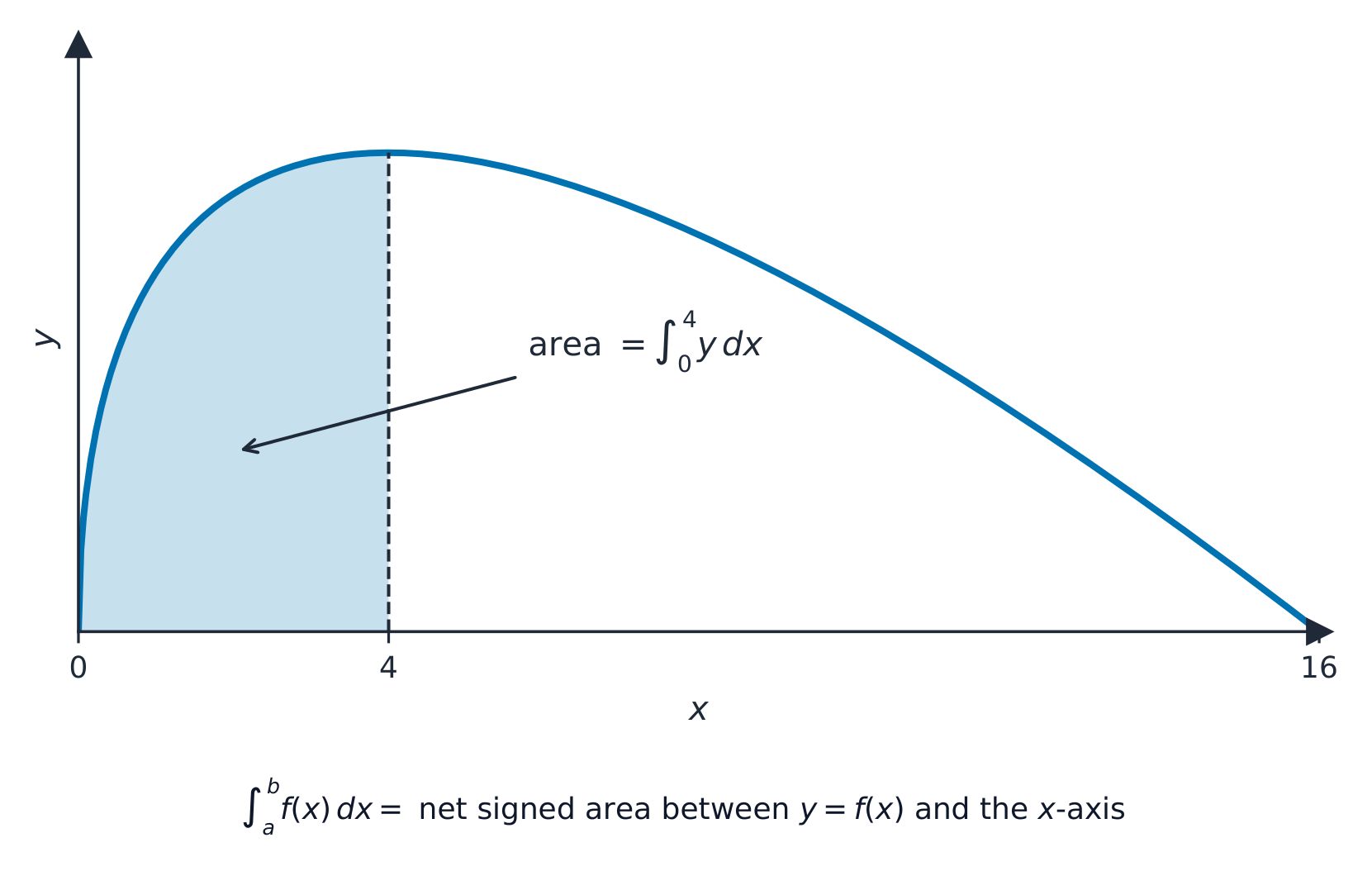
$$\int_p^q f(x)\, dx = \big[F(x)\big]_p^q = F(q) - F(p).$$The area of the region 区域 between a curve and the $x$-axis, from $x = p$ to $x = q$, is $\displaystyle\int_p^q y \, dx$. For the area between two curves, integrate (top curve $-$ bottom curve).The definite integral $\int_0^4 y\,dx$ is the shaded area under the curve. Worked example. The curve $y = 4x^{1/2} - x$ meets the $x$-axis again at $x = 16$. Find the area between the curve and the $x$-axis from $x = 0$ to $x = 4$.
$$\int_0^4 \left(4x^{1/2} - x\right) dx = \left[\frac{8}{3}x^{3/2} - \frac{x^2}{2}\right]_0^4 = \frac{8}{3}(8) - \frac{16}{2} = \frac{64}{3} - 8 = \frac{40}{3}.$$An improper integral 广义积分 has an infinite limit or an endpoint where the integrand is undefined; evaluate it as a limit. For example,
$$\int_1^{\infty}x^{-2}\, dx=\lim_{b\to\infty}\left[-\frac1x\right]_1^{b}=\lim_{b\to\infty}\left(1-\frac1b\right)=1,$$and $\displaystyle\int_0^{1}x^{-1/2}\, dx=\left[2x^{1/2}\right]_0^{1}=2$, which is finite even though the integrand blows up at $x=0$.Volume of revolution
When a region is turned all the way around an axis it sweeps out a solid. The volume of revolution 旋转体体积 about the $x$-axis is
$$V = \pi \int_p^q y^2 \, dx,$$and about the $y$-axis it is $V = \pi \displaystyle\int x^2 \, dy$. For example, the region under $y = \sqrt{x}$ from $x = 0$ to $x = 4$, turned about the $x$-axis, has volume $\pi\displaystyle\int_0^4 x\, dx = \pi\big[\tfrac{x^2}{2}\big]_0^4 = 8\pi$.
Rotating the region under a curve around the $x$-axis sweeps out a solid; each thin slice is a disc of area $\pi y^2$, so $V = \pi\int y^2\,dx$ 탐색하기곡선 아래 면적
y = ax³ + bx² + cx + d
한계를 드래그하세요. 정적분(definite integral) 은 곡선과 x축 사이의 채워진 면적입니다.
어휘 연습하기English 한국어 Integration/ˌɪntɪˈɡreɪʃn/ 적분(integration) constant of integration/ˈkɒnstənt ɒv ˌɪntɪˈɡreɪʃn/ 적분 상수 definite integral/ˈdefɪnət ˈɪntɪɡrəl/ 정적분 region/ˈriːdʒn/ 지역(region) improper integral/ɪmˈprɒpə ˈɪntɪɡrəl/ 부정적분 volume of revolution/ˈvɒljuːm ɒv ˌrevəˈluːʃn/ 회전체적 1.8
Exam tips
- Show every line of algebra — method marks are lost by jumping steps; use the discriminant $b^2 - 4ac$ to decide the number of real roots.
- Work in radians for circular measure (arc $= r\theta$, sector area $= \frac{1}{2}r^2\theta$) and for calculus of trig functions.
- For differentiation, set $\frac{dy}{dx} = 0$ for stationary points and use the second derivative to classify them.
- For integration, add $+ c$ to an indefinite integral and use limits for area; an area below the axis gives a negative integral.
어휘 연습하기English 한국어 algebra/ˈældʒɪbrə/ 대수 calculus/ˈkælkjʊləs/ 미적분 -
2
순수 수학 2
수업 보기이 시트에는 Topic 2: 순수 수학(Pure Mathematics) 2이 다룹니다. 절대값 및 다항대수, 로그함수와 지수함수, 추가 삼각함수, 그리고 미분 및 적분의 새로운 방법을 포함합니다.
2.1
대수학
Syllabus
Candidates should be able to: Notes and examples understand the meaning of $|x|$, sketch the graph of $y = |ax + b|$ and use relations such as $|a| = |b| \iff a^2 = b^2$ and $|x - a| < b \iff a - b < x < a + b$ when solving equations and inequalities Graphs of $y = |f(x)|$ and $y = f(|x|)$ for non-linear functions $f$ are not included. e.g. $|3x - 2| = |2x + 7|$, $2x + 5 < |x + 1|$ divide a polynomial, of degree not exceeding 4, by a linear or quadratic polynomial, and identify the quotient and remainder (which may be zero) use the factor theorem and the remainder theorem. e.g. to find factors and remainders, solve polynomial equations or evaluate unknown coefficients. Including factors of the form $(ax + b)$ in which the coefficient of $x$ is not unity, and including calculation of remainders. 출처: Cambridge International syllabus
절대값
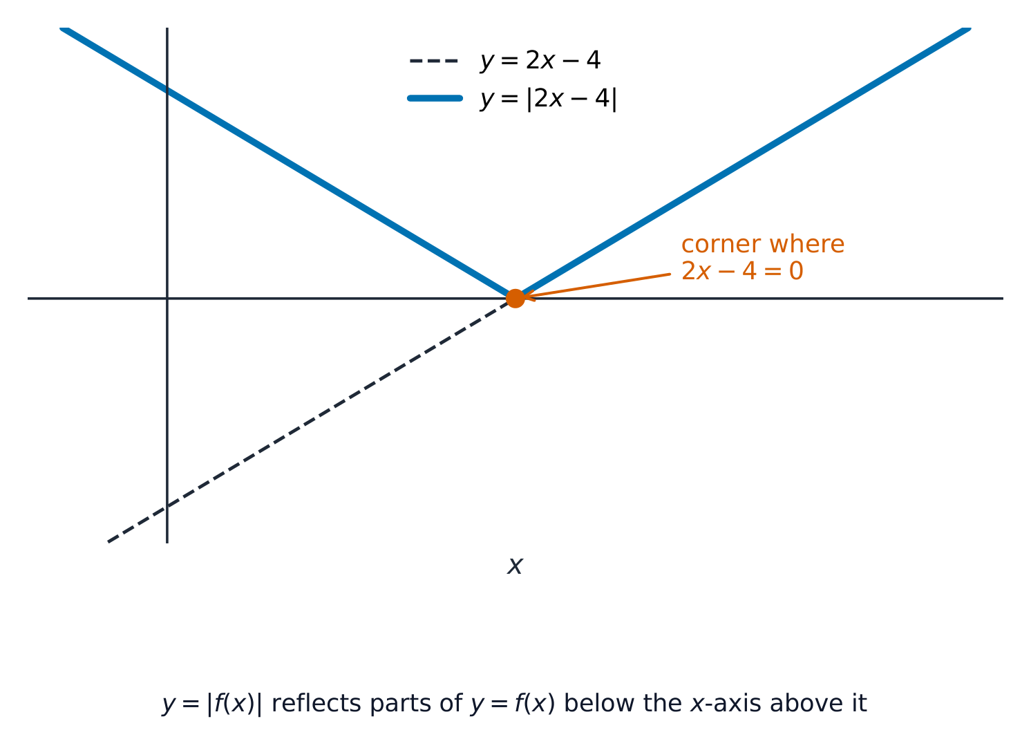
절대값 $|x|$은 부호를 제거한 수의 크기이므로, $|x| \geqslant 0$는 항상 양수입니다. $y = |ax + b|$의 그래프는 $x$-축에서 튀어 오르는 'V'자 형태입니다. 방정식과 부등식을 푸는 데 유용한 두 가지 규칙은 다음과 같습니다.
$$|a| = |b| \;\Leftrightarrow\; a^2 = b^2, \qquad |x - a| < b \;\Leftrightarrow\; a - b < x < a + b.$$절대값을 취하면 축 아래쪽의 선 부분을 위쪽으로 접어 V자를 만듭니다. 풀이 예제. $|3x + 8| < 9$을 풀이하시오.
두 번째 규칙을 inequality를 $-9 < 3x + 8 < 9$로 작성하여 적용합니다:
$$-9 < 3x + 8 < 9 \;\Rightarrow\; -17 < 3x < 1 \;\Rightarrow\; -\tfrac{17}{3} < x < \tfrac13.$$다항식 나눗셈 및 약수 정리와 나머지의 정리
다항식은 $x$의 거듭제곱들의 합으로, 예시로 $2x^4 + 3x^2 - 5$가 있습니다. 차수(degree) 는 가장 높은 거듭제곱입니다. 하나의 다항식을 다른 다항식으로 나누면 비(quotient) 와 나머지(remainder) 를 얻습니다.
- 나머지의 정리: $p(x)$을 $(x - a)$로 나눈 나머지는 $p(a)$입니다.
- 약수 정리: $(x - a)$이 $p(x)$의 약수인 것은 $p(a) = 0$일 때뿐입니다.
작업 예시. 다항식 $p(x) = 2x^4 + kx^3 + kx^2 + 17x + 18$에 약수 $(x + 2)$이 있습니다. $k$를 구하십시오.
약수 정리에 의해 $p(-2) = 0$:
$$2(16) + k(-8) + k(4) + 17(-2) + 18 = 0 \;\Rightarrow\; 16 - 4k = 0 \;\Rightarrow\; k = 4.$$탐색하기절댓값 함수
y = a|x − b| + c
절댓값은 V자 모양을 만든다. 꼭짓점을 b와 c로 이동시키고, 팔의 경사도를 a로 변경한다.
어휘 연습하기English 한국어 Pure Mathematics/pjʊə ˌmæθɪˈmætɪks/ 순수 수학(Pure Mathematics) logarithms/ˈlɒɡərɪθəmz/ 로그(logarithms) exponential function/ˌekspəˈnenʃl ˈfʌŋkʃn/ 지수 함수 modulus/ˈmɒdjʊləs/ 절댓값(모듈러스) polynomial/ˌpɒlɪˈnəʊmɪəl/ 다항함수 degree/dɪˈɡriː/ 차Unless degree (polynomial) or 각도Unless angle. Given mathematical list, likely polynomial degree. quotient/ˈkwəʊʃənt/ 상수항Unless context implies quotient in division. In math context with remainder, it's quotient. remainder/rɪˈmeɪndə/ 나머지 remainder theorem/rɪˈmeɪndə ˈθɪərəm/ 餘定理(나머지 정리) factor theorem/ˈfæktə ˈθɪərəm/ 인수 정리 2.2
로그함수와 지수함수

Syllabus
Candidates should be able to: Notes and examples understand the relationship between logarithms and indices, and use the laws of logarithms (excluding change of base) understand the definition and properties of $e^x$ and $\ln x$, including their relationship as inverse functions and their graphs Including knowledge of the graph of $y = e^{kx}$ for both positive and negative values of $k$. use logarithms to solve equations and inequalities in which the unknown appears in indices e.g. $2^x < 5$, $3 \times 2^{3x-1} < 5$, $3^{x+1} = 4^{2x-1}$ use logarithms to transform a given relationship to linear form, and hence determine unknown constants by considering the gradient and/or intercept. e.g. $y = kx^n$ gives $\ln y = \ln k + n \ln x$ which is linear in $\ln x$ and $\ln y$ $y = k(a^x)$ gives $\ln y = \ln k + x \ln a$ which is linear in $x$ and $\ln y$. 출처: Cambridge International syllabus
지진의 세기는 로그 스케일인 리히터スケール로 측정됩니다. 
자원이 풍부할 때 인구는 지수적으로 증가할 수 있습니다. 로그함수는 "어떤 지수인가?"라는 질문에 답합니다. $a^x = y$이면 $x = \log_a y$입니다. 로그함수와 지수(indices, 거듭제곱) 은 서로 반대되는 개념입니다. 로그의 법칙은 다음과 같습니다.
$$\log(mn) = \log m + \log n, \qquad \log\!\frac{m}{n} = \log m - \log n, \qquad \log(m^k) = k\log m.$$지수함수 $e^x$과 자연로그 $\ln x$는 역함수이므로, $\ln(e^x) = x$이고 $e^{\ln x} = x$입니다. 미지수가 지수에 있는 경우 양변의 로그를 취합니다.
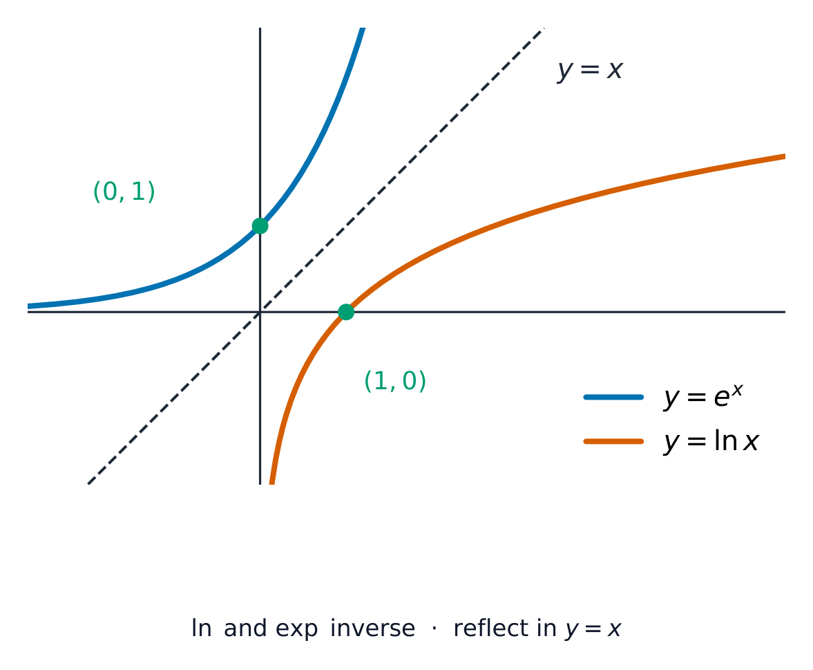
$e^x$과 $\ln x$는 서로 상쇄하므로, 각각 $y=x$에 대해 반사된 것입니다. 풀이 예제. $4^x < 0.05$을 풀이하시오.
$$4^x < 0.05 \;\Rightarrow\; x\ln 4 < \ln 0.05 \;\Rightarrow\; x < \frac{\ln 0.05}{\ln 4} = -2.16 \ (\text{ 유효숫자 3자리}).$$선형 형태: $y = Ax^n$과 같은 관계에서 로그를 취하면 직선이 됩니다: $\ln y = \ln A + n\ln x$. $\ln y$를 $\ln x$에 대해 plot하면 기울기가 $n$이고 절편이 $\ln A$인 직선이 되므로, 미지수 상수를 찾을 수 있습니다.
탐색하기지수 성장
y = a·bˣ
근본 b를 변경하면: b > 1일 때 곡선은 성장하고, 0 < b < 1일 때는 감소하며, 항상 (0, a)를 지나간다.
어휘 연습하기English 한국어 indices/ˈɪndɪsiːz/ 지수 laws of logarithms/lɔːz ɒv ˈlɒɡərɪθəmz/ 로그의 법칙 natural logarithm/ˈnætʃərəl ˈlɒɡərɪθəm/ 자연 로그 linear form/ˈlɪnɪə fɔːm/ 선형 형태 2.3
삼각함수

Syllabus
지원자는 다음을 할 수 있어야 한다: 참고 사항 및 예시 코사인, 코세cant 및 코타젱트 함수가 코사인, 사인, 탄젠트 함수와 어떤 관계가 있는지 이해하고, 임의의 크기의 각에 대한 6가지 삼각함수의 성질과 그래프를 사용한다. 식의 단순화와 정확한 평가를 위해, 그리고 방정식을 풀 때 삼각함수 항등식을 사용하고, 문맥에 적합한 항등식을 선택하며, 특히 다음 사용에 익숙함을 보여준다: – $\sec^2 \theta \equiv 1 + \tan^2 \theta$ 및 $\csc^2 \theta \equiv 1 + \cot^2 \theta$ – $\sin(A \pm B)$, $\cos(A \pm B)$ 및 $\tan(A \pm B)$의 전개식 – $\sin 2A$, $\cos 2A$ 및 $\tan 2A$의 공식 – $a \sin \theta + b \cos \theta$를 $R \sin(\theta \pm \alpha)$ 및 $R \cos(\theta \pm \alpha)$ 형태로 표현함. 예: $\cos(x - 30^\circ) - 3 \sin(x - 60^\circ)$을 단순화함. 예: $\tan \theta + \cot \theta = 4$, $2 \sec^2 \theta - \tan \theta = 5$, $3 \cos \theta + 2 \sin \theta = 1$를 풀이함. 출처: Cambridge International syllabus
더러운 세 개의 함수가 있으며, 모두 아는 함수의 역함수입니다: 세컨트(secant) $\sec\theta = \dfrac{1}{\cos\theta}$, 코세cant(cosecant) $\csc\theta = \dfrac{1}{\sin\theta}$, 그리고 코탄젠트(cotangent) $\cot\theta = \dfrac{1}{\tan\theta}$입니다.
$\sec\theta=1/\cos\theta$은 $\cos\theta=0$일 때마다 극한선으로 상승합니다. 이 삼각함수 항등식들을 기억하고 각 문제에 맞는 것을 선택해야 합니다:
$$\sec^2\theta \equiv 1 + \tan^2\theta, \qquad \csc^2\theta \equiv 1 + \cot^2\theta.$$또한 $\sin(A \pm B)$, $\cos(A \pm B)$, $\tan(A \pm B)$에 대한 합각 공식과 이중각 공식을 사용합니다.$$\sin 2A = 2\sin A\cos A, \quad \cos 2A = 2\cos^2 A - 1, \quad \tan 2A = \frac{2\tan A}{1 - \tan^2 A},$$그리고 R공식 $a\sin\theta + b\cos\theta = R\sin(\theta + \alpha)$, 여기서 $R = \sqrt{a^2 + b^2}$이고 $\tan\alpha = \dfrac{b}{a}$입니다.해설 예제. $2\tan^2\theta + 3\sec\theta = 18$에 대한 $-180^\circ < \theta < 180^\circ$의 해를 구하시오.
$\tan^2\theta$을 $\sec^2\theta - 1$로 치환하여 하나의 함수를 얻습니다:
$$2(\sec^2\theta - 1) + 3\sec\theta = 18 \;\Rightarrow\; 2\sec^2\theta + 3\sec\theta - 20 = 0 \;\Rightarrow\; (2\sec\theta - 5)(\sec\theta + 4) = 0.$$따라서 $\sec\theta = \tfrac52$이거나 $\sec\theta = -4$이므로, $\cos\theta = \tfrac25$이거나 $\cos\theta = -\tfrac14$입니다. 해는 $\theta = \pm 66.4^\circ$과 $\theta = \pm 104.5^\circ$입니다.탐색하기단위원
각도를 드래그하여 $\sin$, $\cos$, $\tan$ 간의 관계를 확인하세요. 이는 삼각방정식을 푸는 데 핵심적인 요소입니다.
어휘 연습하기English 한국어 secant/ˈsiːkənt/ 할선 cosecant/ˈkəʊsekənt/ 코세cant함수 cotangent/ˈkəʊtændʒənt/ 코탄젠트함수 trigonometric identities/ˌtrɪɡənəʊˈmetrɪk aɪˈdentɪtiz/ 삼각 항등식(trigonometric identities) compound angle/ˈkɒmpaʊnd ˈæŋɡl/ 합각(formula for compound angle) double angle/ˈdʌbl ˈæŋɡl/ 이중 각 R-formula/ɑː ˈfɔːmjʊlə/ R-공식 2.4
미분법
Syllabus
지원자는 다음을 할 수 있어야 한다: 참고 사항 및 예시 $e^x$, $\ln x$, $\sin x$, $\cos x$, $\tan x$의 미분을 사용하고, 상수배, 합, 차, 합성함수를 처리한다. 곱함수와商的함수의 미분을 수행한다. 예시: $\frac{2x - 4}{3x + 2}$, $x^2 \ln x$, $x e^{1 - x^2}$. 매개변수 또는 암묵적으로 정의된 함수의 첫 번째 미분식을 구하고 사용한다. 예: $x = t - e^{2t}$, $y = t + e^{2t}$. 예: $x^2 + y^2 = xy + 7$. 접선과 수직선에 관한 문제에서 사용 포함. 출처: Cambridge International syllabus
이 표준 미분식을 암기하십시오:
$$\frac{d}{dx}e^x = e^x, \quad \frac{d}{dx}\ln x = \frac{1}{x}, \quad \frac{d}{dx}\sin x = \cos x, \quad \frac{d}{dx}\cos x = -\sin x, \quad \frac{d}{dx}\tan x = \sec^2 x.$$두 함수의 곱이나 비에 대해서는 다음을 사용하십시오:
- 곱의 미분법(product rule): $(uv)' = u'v + uv'$;
- 비의 미분법(quotient rule): $\left(\dfrac{u}{v}\right)' = \dfrac{u'v - uv'}{v^2}$.
곡선이 매개변수 방정식 $x = x(t)$, $y = y(t)$로 주어졌을 때 기울기는 $\dfrac{dy}{dx} = \dfrac{dy/dt}{dx/dt}$입니다. $y$가 명시되지 않고 암묵적으로 정의되었을 때, $x$에 대해 각 항을 미분하고 $y$항에 대해 연쇄 법칙을 적용한 뒤, $\dfrac{dy}{dx}$에 대해 풀이하십시오.
작업 예시. $y = 6x\cos(x^2 + 1)$이 주어졌을 때, $\dfrac{dy}{dx}$을 구하십시오.
$u = 6x$과 $v = \cos(x^2 + 1)$에 대해 곱의 미분법을 사용하고($v$에 대해서는 체인룰을 사용):
$$\frac{dy}{dx} = 6\cos(x^2 + 1) + 6x\cdot\big(-2x\sin(x^2 + 1)\big) = 6\cos(x^2 + 1) - 12x^2\sin(x^2 + 1).$$탐색하기접선과 기울기
y = ax³ + bx² + cx + d
점을 이동하세요: 접선은 해당 x값에서의 미분값입니다. 곡선이 방향을 바꾸는 곳에서는 기울기가 0입니다.
어휘 연습하기English 한국어 product rule/ˈprɒdʌkt ruːl/ 곱의 법칙 quotient rule/ˈkwəʊʃənt ruːl/ 비율의 법칙 parametric equations/ˌpærəˈmetrɪk ɪˈkweɪʒnz/ 매개변수 방정식 implicitly/ɪmˈplɪsɪtli/ 암묵적으로 2.5
적분법
Syllabus
지원자는 다음을 할 수 있어야 한다: 참고 사항 및 예시 '미분의 역과정'이라는 아이디어를 확장하여 $e^{ax + b}$, $\frac{1}{ax + b}$, $\sin(ax + b)$, $\cos(ax + b)$ 및 $\sec^2(ax + b)$의 적분을 포함시킨다. 대입법에 의한 적분의 일반적인 방식에 대한 지식이 필요하지는 않다. 적분 수행 시 삼각함수 관계를 활용한다. 예시: 이중각 공식을 사용하여 $\sin^2 x$ 또는 $\cos^2(2x)$을 적분하는 경우. 사다리꼴 법칙을 이해하고 활용하여 정적분의 값을 추정한다. 간단한 경우 스키치 그래프를 사용하여 사다리꼴 법칙이 과소평가인지 과대평가인지 판별하는 데 활용한다. 출처: Cambridge International syllabus
적분은 미분의 역연산(reverse differentiation) — 새로운 미분식을 모두 거꾸로 하십시오. 복잡한 적분에는 치환법(integration by substitution) (순수 수학 3에서 다룸)이 필요할 수 있습니다. 내부 함수가 선형 $(ax + b)$인 경우:
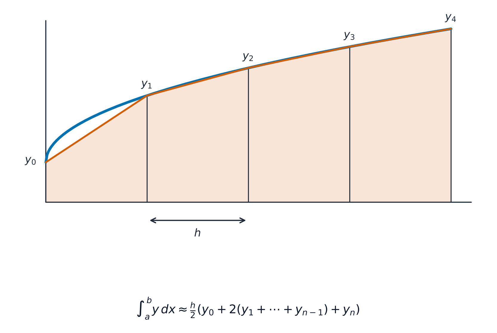
$$\int e^{ax+b}\,dx = \frac{1}{a}e^{ax+b} + C, \qquad \int \frac{1}{ax+b}\,dx = \frac{1}{a}\ln|ax + b| + C,$$$$\int \sin(ax+b)\,dx = -\frac{1}{a}\cos(ax+b) + C, \qquad \int \cos(ax+b)\,dx = \frac{1}{a}\sin(ax+b) + C, \qquad \int \sec^2(ax+b)\,dx = \frac{1}{a}\tan(ax+b) + C.$$$\sin$ 또는 $\cos$의 거듭제곱을 적분하려면, 먼저 항등식을 사용하여 거듭제곱을 제거하십시오. 정확히 적분할 수 없는 경우 사다리꼴 규칙은 정적분의 값을 근사합니다:$$\int_a^b y\,dx \approx \tfrac{h}{2}\big[y_0 + y_n + 2(y_1 + y_2 + \cdots + y_{n-1})\big].$$너비가 $h$인 각 띠는 사다리꼴이며, 이들의 면적을 더하여 적분을 근사합니다. 해설 예제. $\displaystyle\int 6\sin^2 x\,dx$를 구하세요.
$\sin^2 x = \tfrac12(1 - \cos 2x)$를 사용하십시오:
$$\int 6\sin^2 x\,dx = \int (3 - 3\cos 2x)\,dx = 3x - \tfrac32\sin 2x + C.$$탐색하기곡선 아래의 면적
면적 = ∫ f(x) dx
적분은 여전히 면적을 나타냅니다. a와 b를 드래그하여 곡선 아래의 막대 영역을 합산하십시오.
어휘 연습하기English 한국어 trapezium rule/trəˈpiːzɪəm ruːl/ 사다리꼴 규칙 root/ruːt/ 근(루트) integration by substitution/ˌɪntɪˈɡreɪʃn baɪ ˌsʌbstɪˈtjuːʃn/ 대입적분법 2.6
방정식의 수치 해법
Syllabus
지원자는 다음을 할 수 있어야 한다: 참고 사항 및 예시 그래프적 고찰 및/또는 부호 변경 검색을 통해 방정식의 근을 대략적으로 locating한다. 예시: 근이 존재하는 두 연속 정수 쌍을 찾는 경우. 방정식의 근에 수렴하는 근사 수열의 개념을 이해하고, 그 표기법을 사용한다. 주어진 단순 반복 공식 $x_{n + 1} = \text{F}(x_n)$가 해결하려는 방정식과 어떻게 관련되는지 이해하고, 주어진 반복 또는 주어진 방정식의 변형에 기반한 반복을 사용하여 지정된 정확도까지 근을 구할 수 있다. 수렴 조건에 대한 지식은 포함되지 않지만, 반복이 수렴하지 않을 수 있다는 이해는 요구된다. 출처: Cambridge International syllabus
근에 대한 반복: 접선을 타다 많은 방정식은 정확히 풀리지 않습니다. 두 가지 아이디어가 근(해)을 찾는 데 도움이 됩니다.
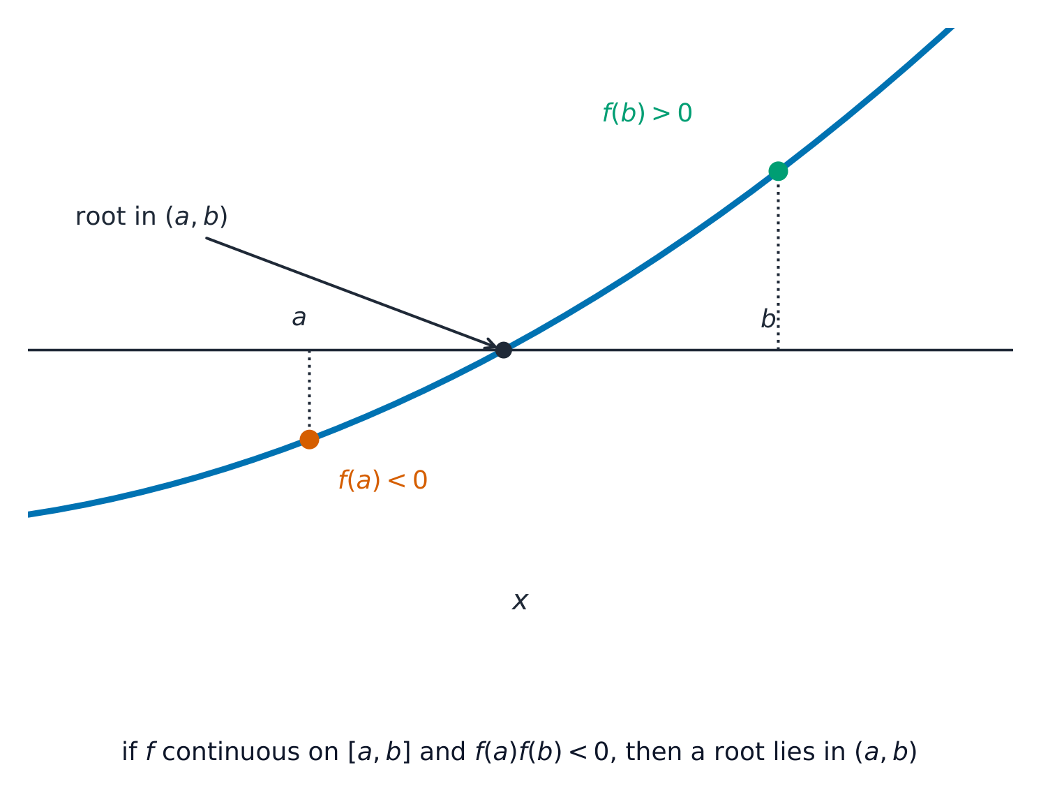
- 부호 변화: $f(a)$와 $f(b)$의 부호가 서로 다르고(그래프 사이에 단절이 없는 경우), 근은 $a$과 $b$ 사이에 존재합니다.
- 반복법: 방정식을 $x = F(x)$ 형태로 변형한 뒤, 반복 공식 $x_{n+1} = F(x_n)$을 사용합니다. 첫 추정치 $x_0$에서 시작하여 반복하십시오. 값들이 수렴하면 안정화되어 근으로 수렴합니다. 요청된 정밀도까지 답이 일정해질 때까지 계속 하십시오.
$f(a)$와 $f(b)$의 부호가 다르므로, 근은 $a$과 $b$ 사이에 존재합니다. 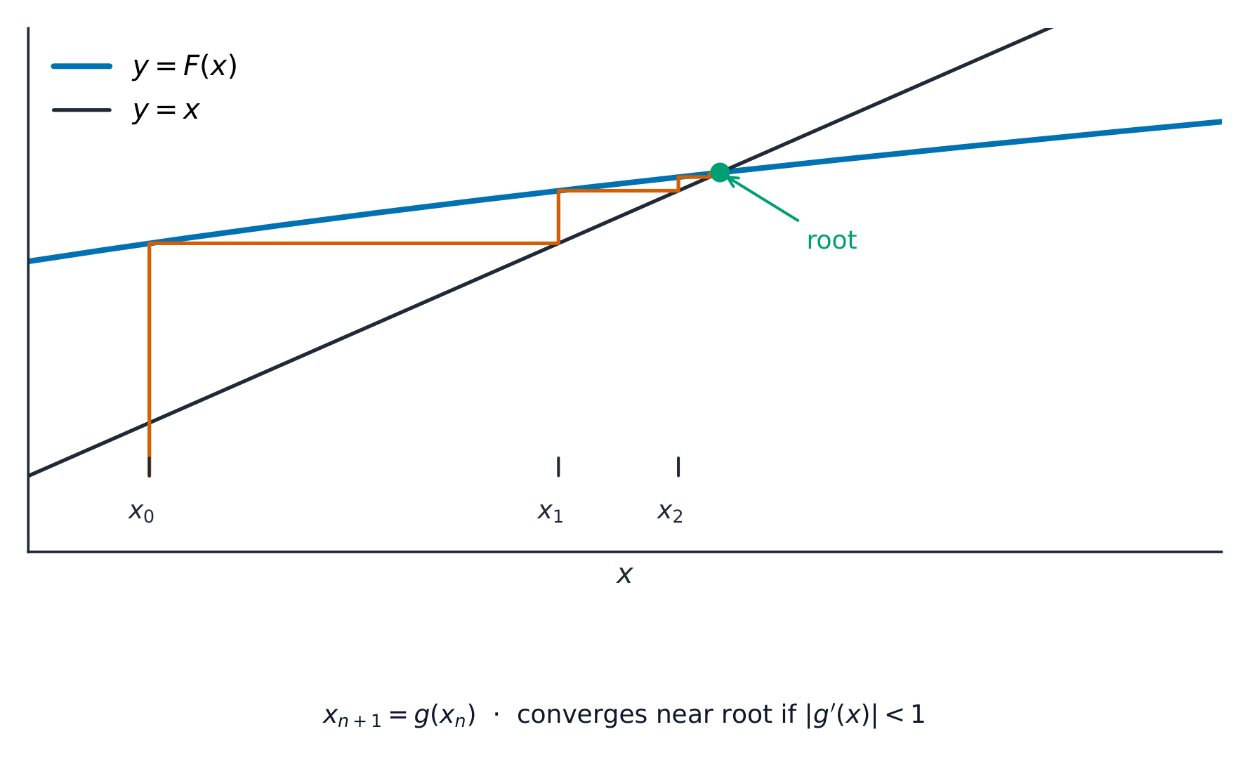
각 단계는 위로 올라가 $y=F(x)$에 도달한 후 가로로 이동하여 $y=x$에 도달합니다; 이 계단은 근에 수렴합니다. 해설 예제. 방정식의 근 $\beta$이 $x = \sqrt[3]{-2x - 4.5}$과 $-1.4 < \beta < -1.0$을 만족한다. 반복 공식 $x_{n+1} = \sqrt[3]{-2x_n - 4.5}$에 $x_0 = -1.2$를 사용하여 구하시오.
$$x_1 = \sqrt[3]{-2(-1.2) - 4.5} = \sqrt[3]{-2.1} = -1.281, \qquad x_2 = \sqrt[3]{-2(-1.281) - 4.5} = -1.247, \quad \ldots$$값들이 $-1.26$ 근처에서 안정화되므로, 답은 (유효숫자 3개) $\beta = -1.26$입니다.탐색하기근(root)은 어디에 있습니까?
y = ax³ + bx² + cx + d
근은 곡선이 0을 가로지르는 지점입니다. f(x)의 **부호 변화(sign change)**는 두 x값 사이에 근이 존재함을 의미합니다.
어휘 연습하기English 한국어 sign change/saɪn tʃeɪndʒ/ 부호 변화 iteration/ˌɪtəˈreɪʃn/ 반복(iteration) iterative formula/ˈɪtərətɪv ˈfɔːmjʊlə/ 반복 공식 converge/kənˈvɜːdʒ/ 수렴 2.6
시험 팁
- 로그의 법칙을 사용하여 방정식을 풀고, $\ln$와 $e^x$이 역함수임을 기억하십시오.
- 수치 방법에서는 근을 찾기 위해 부호 변화를 보여주고, 반복법을 명확히 정리하며, 명시된 정밀도에 따라 답을 제시하십시오.
- 연쇄, 곱 및 나눗의 법칙을 외우고, 함수에 어떤 법칙이 필요한지 식별하십시오.
- 절댓값 방정식 $|f(x)| = g(x)$를 풀 때는 양수 및 음수 경우를 모두 고려하고, 스킷을 그려 확인하십시오.
-
3
순수 수학 3
수업 보기This handout covers Topic 3: Pure Mathematics 纯数学 3. Subtopics 3.1–3.6 build on the algebra, logarithms, trigonometry, differentiation, integration and numerical methods of Pure Mathematics 2, so this handout explains what is new in Pure 3 and then covers the three big new areas: vectors, differential equations and complex numbers.
3.1
Algebra
Syllabus
Candidates should be able to: Notes and examples • understand the meaning of $|x|$, sketch the graph of $y = |ax + b|$ and use relations such as $|a| = |b| \iff a^2 = b^2$ and $|x - a| < b \iff a - b < x < a + b$ when solving equations and inequalities Graphs of $y = |\text{f}(x)|$ and $y = \text{f}(|x|)$ for non-linear functions $\text{f}$ are not included. e.g. $|3x - 2| = |2x + 7|$, $2x + 5 < |x + 1|$. • divide a polynomial, of degree not exceeding 4, by a linear or quadratic polynomial, and identify the quotient and remainder (which may be zero) • use the factor theorem and the remainder theorem e.g. to find factors and remainders, solve polynomial equations or evaluate unknown coefficients. Including factors of the form $(ax + b)$ in which the coefficient of $x$ is not unity, and including calculation of remainders. • recall an appropriate form for expressing rational functions in partial fractions, and carry out the decomposition, in cases where the denominator is no more complicated than – $(ax + b)(cx + d)(ex + f)$ – $(ax + b)(cx + d)^2$ – $(ax + b)(cx^2 + d)$ Excluding cases where the degree of the numerator exceeds that of the denominator • use the expansion of $(1 + x)^n$, where $n$ is a rational number and $|x| < 1$. Finding the general term in an expansion is not included. Adapting the standard series to expand e.g. $(2 - \frac{1}{2}x)^{-1}$ is included, and determining the set of values of $x$ for which the expansion is valid in such cases is also included. 출처: Cambridge International syllabus
Two new tools join the algebra from Pure 2.
Partial fractions
A single fraction with a factorised bottom can be split into a sum of simpler fractions. This is called writing it in partial fractions 部分分式, and it makes a rational function 有理函数 (a fraction of polynomials) easy to integrate or expand. Match the form to the bottom:
First check the top is lower degree than the bottom. If it is not ("top-heavy"), divide the polynomial first: dividing gives a quotient 商 plus a remainder 余数 over the original bottom, and you split only that remaining proper fraction.
One fraction with a factorised bottom splits into a sum of simpler fractions.
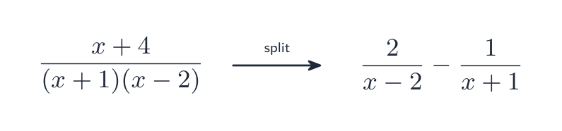
$$\frac{1}{(ax+b)(cx+d)} = \frac{A}{ax+b} + \frac{B}{cx+d}, \qquad \frac{1}{(ax+b)(cx+d)^2} = \frac{A}{ax+b} + \frac{B}{cx+d} + \frac{C}{(cx+d)^2}.$$Worked example. Express $\dfrac{x+4}{(x+1)(x-2)}$ in partial fractions.
Write $\dfrac{x+4}{(x+1)(x-2)} = \dfrac{A}{x+1} + \dfrac{B}{x-2}$, so $x + 4 = A(x-2) + B(x+1)$. Put $x = 2$: $6 = 3B$, so $B = 2$. Put $x = -1$: $3 = -3A$, so $A = -1$. Hence
$$\frac{x+4}{(x+1)(x-2)} = \frac{2}{x-2} - \frac{1}{x+1}.$$The binomial expansion for a rational power
The binomial expansion 二项展开式 also works when the power is a fraction or is negative, as long as $|x| < 1$:
$$(1 + x)^n = 1 + nx + \frac{n(n-1)}{2!}x^2 + \frac{n(n-1)(n-2)}{3!}x^3 + \cdots$$For example $(1 + x)^{1/2} = 1 + \tfrac12 x - \tfrac18 x^2 + \cdots$ for $|x| < 1$.탐색하기역함수 곡선(reciprocal curves)
y = a/(x − b) + c
부분분수 분해(partial fractions)는 어려운 분수를 간단한 역함수 조각으로 나누어, 각각 수직 및 수평 점근선을 가질 수 있게 합니다.
어휘 연습하기English 한국어 Pure Mathematics/pjʊə ˌmæθɪˈmætɪks/ 순수 수학(Pure Mathematics) partial fractions/ˈpɑːʃl ˈfrækʃnz/ 부분분수 분해를 사용 rational function/ˈræʃənl ˈfʌŋkʃn/ 유계 함수 quotient/ˈkwəʊʃənt/ 상수항Unless context implies quotient in division. In math context with remainder, it's quotient. remainder/rɪˈmeɪndə/ 나머지 binomial expansion/baɪˈnəʊmɪəl ekˈspænʃn/ 이항 전개 3.2 3.3 3.6
Logarithms, trigonometry and numerical methods (from Pure 2)
Syllabus
Candidates should be able to: Notes and examples understand the relationship between logarithms and indices, and use the laws of logarithms (excluding change of base) understand the definition and properties of $e^x$ and $\ln x$, including their relationship as inverse functions and their graphs Including knowledge of the graph of $y = e^{kx}$ for both positive and negative values of $k$. use logarithms to solve equations and inequalities in which the unknown appears in indices e.g. $2^x < 5$, $3 \times 2^{3x-1} < 5$, $3^{x+1} = 4^{2x-1}$. use logarithms to transform a given relationship to linear form, and hence determine unknown constants by considering the gradient and/or intercept. e.g. $y = kx^n$ gives $\ln y = \ln k + n \ln x$ which is linear in $\ln x$ and $\ln y$. $y = k(a^x)$ gives $\ln y = \ln k + x \ln a$ which is linear in $x$ and $\ln y$. 지원자는 다음을 할 수 있어야 한다: 참고 사항 및 예시 코사인, 코세cant 및 코타젱트 함수가 코사인, 사인, 탄젠트 함수와 어떤 관계가 있는지 이해하고, 임의의 크기의 각에 대한 6가지 삼각함수의 성질과 그래프를 사용한다. 식의 단순화와 정확한 평가를 위해, 그리고 방정식을 풀 때 삼각함수 항등식을 사용하고, 문맥에 적합한 항등식을 선택하며, 특히 다음 사용에 익숙함을 보여준다: – $\sec^2 \theta \equiv 1 + \tan^2 \theta$ 및 $\cosec^2 \theta \equiv 1 + \cot^2 \theta$ – $\sin(A \pm B)$, $\cos(A \pm B)$ 및 $\tan(A \pm B)$의 전개식 – $\sin 2A$, $\cos 2A$ 및 $\tan 2A$의 공식 – $a \sin \theta + b \cos \theta$를 $R \sin(\theta \pm \alpha)$ 및 $R \cos(\theta \pm \alpha)$ 형태로 표현함. 예: $\cos(x - 30^\circ) - 3 \sin(x - 60^\circ)$을 단순화함. 예: $\tan \theta + \cot \theta = 4$, $2 \sec^2 \theta - \tan \theta = 5$, $3 \cos \theta + 2 \sin \theta = 1$를 풀이함. 지원자는 다음을 할 수 있어야 한다: 참고 사항 및 예시 • 그래프적 고찰 및/또는 부호 변경 탐색을 통해 방정식의 근을 근사적으로 locating한다 예: 근이 존재하는 두 연속 정수를 찾는 것. • 방정식의 근으로 수렴하는 근사값의 순서에 대한 개념을 이해하고, 그 표기법을 사용한다 • 주어진 $x_{n+1} = \text{F}(x_n)$ 형태의 간단한 반복 공식이 해결하려는 방정식과 어떻게 관련되는지 이해하고, 주어진 반복 또는 주어진 방정식의 변형에 기반한 반복을 사용하여 지정된 정확도 수준의 근을 구한다. 수렴에 대한 조건에 대한 지식은 포함되지 않으나, 반복이 수렴하지 않을 수 있다는 점에 대한 이해가 요구된다. 출처: Cambridge International syllabus
Iterating to a root: ride the tangent Subtopics 3.2, 3.3 and 3.6 are the same skills you met in Pure 2: the laws of logarithms with $e^x$ and $\ln x$; the identities $\sec^2\theta \equiv 1 + \tan^2\theta$ and $\csc^2\theta \equiv 1 + \cot^2\theta$, the compound- and double-angle formulae, and the $R$-form of $a\sin\theta + b\cos\theta$; and solving an equation numerically by a sign change 变号 and an iterative formula 迭代公式 $x_{n+1} = F(x_n)$. Use them exactly as before.
The three new trig functions are the reciprocals 倒数 of the familiar ones: the secant 正割 $\sec\theta = \dfrac{1}{\cos\theta}$, the cosecant 余割 $\csc\theta = \dfrac{1}{\sin\theta}$, and the cotangent 余切 $\cot\theta = \dfrac{1}{\tan\theta} = \dfrac{\cos\theta}{\sin\theta}$. (Memory aid: match the third letter — sec goes with cosine.) The two Pythagorean identities above come straight from dividing $\sin^2\theta + \cos^2\theta \equiv 1$ by $\cos^2\theta$ or $\sin^2\theta$. For a numerical method, an iteration $x_{n+1}=F(x_n)$ converges 收敛 to the root when successive values get closer together.
탐색하기단위원
(cos θ, sin θ)
**R공식(R-formula)**은 a sin θ + b cos θ를 하나의 파동으로 변환하며, 모든 과정은 이 원 위에 존재합니다.
어휘 연습하기English 한국어 sign change/saɪn tʃeɪndʒ/ 부호 변화 iterative formula/ˈɪtərətɪv ˈfɔːmjʊlə/ 반복 공식 reciprocals/rɪˈsɪprəklz/ 역수입니다 secant/ˈsiːkənt/ 할선 cosecant/ˈkəʊsekənt/ 코세cant함수 cotangent/ˈkəʊtændʒənt/ 코탄젠트함수 converges/kənˈvɜːdʒɪz/ 수렴함 3.4
Differentiation
Syllabus
지원자는 다음을 할 수 있어야 한다: 참고 사항 및 예시 $e^x$, $\ln x$, $\sin x$, $\cos x$, $\tan x$, $\tan^{-1} x$의 도함수를 상수배, 합, 차이, 합성함수와 함께 사용한다. $\sin^{-1} x$와 $\cos^{-1} x$의 도함수는 불필요하다. 곱함수와 商함수의 미분을 수행한다. 예시: $\frac{2x - 4}{3x + 2}$, $x^2 \ln x$, $x e^{1-x^2}$. 매개변수적 또는 암묵적으로 정의된 함수의 첫 번째 도함수를 구하고 사용한다. 예: $x = t - e^{2t}$, $y = t + e^{2t}$. 예: $x^2 + y^2 = xy + 7$. 접선과 법선에 관련된 문제에서의 사용 포함. 출처: Cambridge International syllabus
The methods are those of Pure 2 (the product, quotient and chain rules, with parametric and implicit curves). One derivative is added — the inverse tangent 反正切:
$$\frac{d}{dx}\tan^{-1} x = \frac{1}{1 + x^2}.$$Worked example. Differentiate $y = \tan^{-1}(3x)$.
Use the chain rule with the result above: $\dfrac{dy}{dx} = \dfrac{1}{1 + (3x)^2} \times 3 = \dfrac{3}{1 + 9x^2}.$
탐색하기한 점에서의 기울기
기울기 = dy/dx
암묵적 미분이든 명시적 미분이든, 미분계수는 여전히 접선의 기울기입니다. 점을 이동하여 확인해 보십시오.
어휘 연습하기English 한국어 inverse tangent/ɪnˈvɜːs ˈtændʒənt/ 역접선 3.5
Integration
Syllabus
Candidates should be able to: Notes and examples extend the idea of 'reverse differentiation' to include the integration of $e^{ax + b}$, $\frac{1}{ax + b}$, $\sin(ax + b)$, $\cos(ax + b)$, $\sec^2(ax + b)$ and $\frac{1}{x^2 + a^2}$ Including examples such as $\frac{1}{2 + 3x^2}$. use trigonometrical relationships in carrying out integration e.g. use of double-angle formulae to integrate $\sin^2 x$ or $\cos^2(2x)$. integrate rational functions by means of decomposition into partial fractions Restricted to types of partial fractions as specified in topic 3.1 above. recognise an integrand of the form $\frac{k f'(x)}{f(x)}$, and integrate such functions e.g. integration of $\frac{x}{x^2 + 1}$, $\tan x$. recognise when an integrand can usefully be regarded as a product, and use integration by parts e.g. integration of $x \sin 2x$, $x^2 e^{-x}$, $\ln x$, $x \tan^{-1} x$. use a given substitution to simplify and evaluate either a definite or an indefinite integral. e.g. to integrate $\sin^2 2x \cos x$ using the substitution $u = \sin x$. 출처: Cambridge International syllabus
Pure 3 adds several powerful methods.
- A new standard integral: $\displaystyle\int \frac{1}{x^2 + a^2}\,dx = \frac{1}{a}\tan^{-1}\frac{x}{a} + C$.
- Partial fractions: split a rational function first, then integrate each piece as a logarithm.
- The pattern $\dfrac{k\,f'(x)}{f(x)}$: this integrates to $k\ln|f(x)| + C$. For example $\displaystyle\int \frac{2x}{x^2 + 1}\,dx = \ln(x^2 + 1) + C$.
- Integration by parts 分部积分, used for a product: $\displaystyle\int u\,\frac{dv}{dx}\,dx = uv - \int v\,\frac{du}{dx}\,dx$.
- Integration by substitution 换元积分: a given change of variable turns a hard integral into an easy one.
Worked example. Find $\displaystyle\int x\cos x\,dx$.
Use integration by parts with $u = x$ and $\dfrac{dv}{dx} = \cos x$, so $\dfrac{du}{dx} = 1$ and $v = \sin x$:
$$\int x\cos x\,dx = x\sin x - \int \sin x\,dx = x\sin x + \cos x + C.$$탐색하기곡선 아래의 면적
면적 = ∫ f(x) dx
모든 적분 방법은 이 면적을 측정하는 것입니다 — 한계를 드래그하여 합산하세요.
어휘 연습하기English 한국어 Integration by parts/ˌɪntɪˈɡreɪʃn baɪ pɑːts/ 부분 적분 Integration by substitution/ˌɪntɪˈɡreɪʃn baɪ ˌsʌbstɪˈtjuːʃn/ 치환적 적분(Integration by substitution) 3.7
Vectors

Syllabus
지원자는 다음을 할 수 있어야 한다: 참고 사항 및 예시 • 표준 벡터 표기법, 즉 $\begin{pmatrix} x \\ y \end{pmatrix}$, $x\mathbf{i} + y\mathbf{j}$, $\begin{pmatrix} x \\ y \\ z \end{pmatrix}$, $x\mathbf{i} + y\mathbf{j} + z\mathbf{k}$, $\overrightarrow{AB}$, $\mathbf{a}$을 사용한다 • 벡터의 덧셈과 뺄셈, 그리고 스칼라에 의한 벡터의 스칼라배를 수행하고, 기하학적 관점에서 이 연산을 해석한다 예: ‘$OABC$는 평행사변형이다’는 $\overrightarrow{OB} = \overrightarrow{OA} + \overrightarrow{OC}$과 동치이다. 비율 정리의 일반형은 포함되지 않으나, $AB$의 중점이 위치 벡터 $\frac{1}{2}(\overrightarrow{OA} + \overrightarrow{OB})$임을 이해하는 것이 요구된다. • 벡터의 **크기(모듈)**를 계산하고, 단위 벡터, 이동 벡터 및 위치 벡터를 사용한다 2차원 또는 3차원에서. • 직선의 방정식이 $\mathbf{r} = \mathbf{a} + t\mathbf{b}$ 형태로 표현될 때 사용되는 모든 기호의 의미를 이해하고, 충분한 정보가 주어졌을 때 직선의 방정식을 구한다 예: 직선 위의 한 점의 위치 벡터와 방향 벡터를 주거나, 직선 위의 두 점의 위치 벡터를 주어 직선의 방정식을 구하는 경우. • 두 직선이 평행인지, 교차하는지, 혹은 **일직선上不共面(异面直线)**인지를 판별하고, 두 직선의 교점을 찾을 수 있을 때 이를 구한다 두 일직선上不共面(异面直线) 사이의 최단 거리 계산은 불필요하다. 두 일직선上不共面(异面直线)에 대한 공통 수직선의 방정식을 구하는 것도 불필요하다. • 두 벡터의 내적을 계산하는 공식을 사용하고, 내적을 직선과 점 관련 문제에서 활용한다. 예: 두 직선 사이의 각도를 구하거나, 한 점에서 직선으로 내린 수선의 발을 구하는 것; 질문에는 사육면체, 사면체(피라미드) 등의 3D 객체가 포함될 수 있다. 외적에 대한 지식은 불필요하다. 출처: Cambridge International syllabus
Forces like wind and water are vectors — they have both size and direction. A vector 向量 has both size and direction. Write it as a column, or as $x\mathbf{i} + y\mathbf{j} + z\mathbf{k}$, or as $\overrightarrow{AB}$.
- The magnitude 模长 (length) of $\mathbf{v} = x\mathbf{i} + y\mathbf{j} + z\mathbf{k}$ is $|\mathbf{v}| = \sqrt{x^2 + y^2 + z^2}$.
- A unit vector 单位向量 has magnitude $1$; divide a vector by its magnitude to make one.
- A position vector 位置向量 gives a point's place from the origin; a displacement vector 位移向量 $\overrightarrow{AB} = \mathbf{b} - \mathbf{a}$ goes from one point to another. Multiplying by a scalar 标量 (a plain number) stretches a vector.
Lines and the scalar product
A straight line through point $\mathbf{a}$ in direction $\mathbf{b}$ has vector equation $\mathbf{r} = \mathbf{a} + t\mathbf{b}$. Two lines may be parallel 平行, may intersect 相交 at a point, or may be skew lines 异面直线 (not parallel and never meeting).

Start at the point $\mathbf{a}$, then add $t$ copies of the direction $\mathbf{b}$ to reach any point on the line. The scalar product 数量积 (dot product) of $\mathbf{a}$ and $\mathbf{b}$ is
$$\mathbf{a}\cdot\mathbf{b} = a_1 b_1 + a_2 b_2 + a_3 b_3 = |\mathbf{a}|\,|\mathbf{b}|\cos\theta,$$where $\theta$ is the angle between them. So $\mathbf{a}\cdot\mathbf{b} = 0$ means the vectors are perpendicular.
The scalar product picks out $|\mathbf{b}|\cos\theta$, how far $\mathbf{b}$ reaches along $\mathbf{a}$. Worked example. Find the angle between $\mathbf{a} = \mathbf{i} + 2\mathbf{j} + 2\mathbf{k}$ and $\mathbf{b} = 2\mathbf{i} + 2\mathbf{j} + \mathbf{k}$.
$$\mathbf{a}\cdot\mathbf{b} = (1)(2) + (2)(2) + (2)(1) = 8, \qquad |\mathbf{a}| = |\mathbf{b}| = 3.$$So $\cos\theta = \dfrac{8}{3\times 3} = \dfrac{8}{9}$, giving $\theta = 27.3^\circ$.탐색하기ベクトル 덧셈과 내적 dot product
두 벡터를 드래그하세요. 합성 벡터(resultant) (끝에서 끝으로)와 내적을 확인하세요. 두 벡터가 서로 수직일 때 내적은 0입니다.
어휘 연습하기English 한국어 vector/ˈvektə/ 벡터 magnitude/ˈmæɡnɪtjuːd/ 크기 unit vector/ˈjuːnɪt ˈvektə/ 단위 벡터 position vector/pəˈzɪʃn ˈvektə/ 위치 벡터 displacement vector/dɪˈspleɪsmənt ˈvektə/ 변위 벡터(displacement vector) scalar/ˈskeɪlə/ 스칼라 parallel/ˈpærəlel/ 평행 intersect/ˌɪntəˈsekt/ 교차하다 skew lines/skjuː laɪnz/ 이 skew 선(skew lines) scalar product/ˈskeɪlə ˈprɒdʌkt/ 스칼라 곱 3.8
Differential equations

Syllabus
Candidates should be able to: Notes and examples formulate a simple statement involving a rate of change as a differential equation The introduction and evaluation of a constant of proportionality, where necessary, is included. find by integration a general form of solution for a first order differential equation in which the variables are separable Including any of the integration techniques from topic 3.5 above. use an initial condition to find a particular solution interpret the solution of a differential equation in the context of a problem being modelled by the equation. Where a differential equation is used to model a 'real-life' situation, no specialised knowledge of the context will be required. 출처: Cambridge International syllabus
A differential equation 微分方程 links a quantity to its rate of change. To solve a first-order equation whose variables are separable 可分离变量, put all the $y$ terms on one side and all the $x$ terms on the other, then integrate both sides. This gives the general solution 通解, which contains a constant. An initial condition 初始条件 (a known value) fixes the constant and gives the particular solution 特解.
Worked example. Solve $\dfrac{dy}{dx} = xy$, given that $y = 1$ when $x = 0$.
Separate the variables and integrate:
$$\int \frac{1}{y}\,dy = \int x\,dx \;\Rightarrow\; \ln y = \tfrac12 x^2 + c \;\Rightarrow\; y = A e^{x^2/2}.$$Using $y = 1$ at $x = 0$ gives $A = 1$, so $y = e^{x^2/2}$.The constant $A$ gives a whole family of curves; the condition $y=1$ at $x=0$ selects $y=e^{x^2/2}$. 탐색하기경향장 slope field
작은 선들이 그 지점에서의 기울기 $\frac{dy}{dx}$를 나타냅니다. 해 곡선(solution curve) 은 화살표를 따라 이동하므로 시작점을 변경하여 다른 해를 볼 수 있습니다.
어휘 연습하기English 한국어 differential equation/ˌdɪfəˈrenʃl ɪˈkweɪʒn/ 미분 방정식 separable/ˈsepərəbl/ 분리 가능하다 general solution/ˈdʒenərəl səˈluːʃn/ 일반 해 initial condition/ɪˈnɪʃl kənˈdɪʃn/ 초기 조건 particular solution/pəˈtɪkjʊlə səˈluːʃn/ 특이해 3.9
Complex numbers

Syllabus
지원자는 다음을 할 수 있어야 한다: 참고 사항 및 예시 복소수의 개념을 이해하고, 실수부, 허수부, 절댓값, 인수(Argument), 복소켤레 등의 용어의 의미를 기억하며, 두 복소수가 실수부와 허수부가 모두 같을 때에만 같다는 사실을 사용한다. 표기법 $\text{Re } z$, $\text{Im } z$, $|z|$, $\arg z$, $z^*$를 알아야 한다. 복소수의 인수는 일반적으로 $\theta$인 각도 $-\pi < \theta \leqslant \pi$를 가리키지만, 어떤 경우에는 구간 $0 \leqslant \theta < 2\pi$가 더 편리할 수 있다. 질문이 명시하지 않는 한 답은 어느 구间을 사용해도 좋다. Cartesian form $x + \text{i}y$로 표시된 두 복소수의 덧셈, 뺄셈, 곱셈, 나눗셈 연산을 수행한다 곱셈이나 나눗셈을 위한 계산 과정의 완전한 세부 내용은 반드시 제시해야 한다. 실수 계수를 가진 다항 방정식에 대해, 비실수 근은 항상 복소켤레 쌍으로 나타난다는 결과를 사용한다 예: one complex root가 주어진 삼차 또는 사차 방정식을 풀 때. Argand diagram을 사용하여 복소수를 기하학적으로 표현한다 polar form $r(\cos \theta + \text{i}\sin \theta) \equiv r\text{e}^{\text{i}\theta}$로 표시된 두 복소수의 곱셈과 나눗셈 연산을 수행한다 결과 $|z_1 z_2| = |z_1||z_2|$과 $\arg(z_1 z_2) = \arg(z_1) + \arg(z_2)$, 그리고 나눗셈에 대한 대응 결과를 포함한다. 복소수의 두 제곱근을 구한다 예: Exact Cartesian form으로 $5 + 12\text{i}$의 제곱근을 구하는 것. 계산 과정의 완전한 세부 내용은 반드시 제시해야 한다. 복소수의 켤레를 취하는 것, 그리고 두 복소수를 더하거나 빼고, 곱하거나 나누는 것의 기하학적 효과를 간략히 이해한다 Argand diagram에서의 **ember(轨迹)**를 사용하여 복소수에 관한 간단한 방정식과 부등식을 시각화한다 예: $|z - a| < k$, $|z - a| = |z - b|$, $\arg(z - a) = \alpha$. 출처: Cambridge International syllabus
Multiplying complex numbers: lengths multiply, angles add Multiplying by i is a rotation Self-similar patterns like Romanesco arise from iterating functions in the complex plane. A complex number 复数 has the form $z = x + iy$, where $i^2 = -1$. Here $x$ is the real part 实部 and $y$ is the imaginary part 虚部. This $x + iy$ is the Cartesian form 直角坐标形式. Two complex numbers are equal only when their real parts match and their imaginary parts match.
- The conjugate 共轭 of $z = x + iy$ is $z^* = x - iy$. For a polynomial with real coefficients, any non-real roots come in conjugate pairs.
- The modulus 模 is $|z| = \sqrt{x^2 + y^2}$ (its distance from the origin) and the argument 辐角 is the angle the point makes, measured from the positive real axis.
- You can plot $z$ as a point on an Argand diagram 阿干图 (the complex plane).
- The polar form 极坐标形式 is $z = r(\cos\theta + i\sin\theta) = re^{i\theta}$, where $r = |z|$ and $\theta$ is the argument. Multiplying multiplies the moduli and adds the arguments.
- The loci of points satisfying a condition on $z$ are drawn on the Argand diagram — e.g. $|z - a| = r$ is a circle, $|z - a| = |z - b|$ a perpendicular bisector, and $\arg(z - a) = \theta$ a half-line. The square roots of a complex number come from solving $w^2 = z$.

On the Argand diagram $|z|$ is the distance from $O$, $\arg z$ the angle, and $z^{*}$ the reflection in the real axis. To divide, multiply top and bottom by the conjugate of the bottom.
Worked example. Write $\dfrac{3 + i}{1 - i}$ in the form $x + iy$.
$$\frac{3 + i}{1 - i} = \frac{(3 + i)(1 + i)}{(1 - i)(1 + i)} = \frac{3 + 3i + i + i^2}{1 + 1} = \frac{2 + 4i}{2} = 1 + 2i.$$An equation or inequality in $z$ describes a locus 轨迹 (a path or region) on the Argand diagram. For example $|z - a| = r$ is a circle of radius $r$ centred at $a$.

$|z-a|=r$ is the set of points a fixed distance $r$ from $a$ — a circle. 탐색하기아르간도 도표
점을 드래그하세요. 복소수 $a + bi$는 평면상의 점이며, 절댓값(modulus) 은 원점으로부터의 거리, 인자(argument) 은 각도입니다.
어휘 연습하기English 한국어 complex number/ˈkɒmpleks ˈnʌmbə/ 복소수 real part/rɪəl pɑːt/ 실수부 imaginary part/ɪˈmædʒɪnəri pɑːt/ 허수부 Cartesian form/kɑːˈtiːzɪən fɔːm/ 카르테esian 형태(Cartesian form) conjugate/ˈkɒndʒuːɡeɪt/ 상쇄 산/염기 modulus/ˈmɒdjʊləs/ 절댓값(모듈러스) argument/ˈɑːɡjuːmənt/ 인자(argument) Argand diagram/ˈɑːɡænd ˈdaɪəɡræm/ 아르당 도표 polar form/ˈpəʊlə fɔːm/ 극좌표 형식 locus/ˈləʊkəs/ ember 3.9
Exam tips
- Split a rational function into partial fractions before integrating or expanding.
- Choose the right integration technique (substitution, by parts, or partial fractions) from the form of the integrand.
- Use the scalar (dot) product for the angle between vectors and to test for perpendicularity; write a line as $\mathbf{r} = \mathbf{a} + t\mathbf{b}$.
- Give complex numbers in the form asked for (Cartesian or modulus-argument) and show them on an Argand diagram.
-
4
역학
수업 보기This handout covers Topic 4: Mechanics 力学. It studies how forces make objects move. Throughout this topic, take the acceleration of free fall as $g = 10\ \text{m s}^{-2}$.
4.1
Forces and equilibrium
Syllabus
Candidates should be able to: Notes and examples identify the forces acting in a given situation e.g. by drawing a force diagram. understand the vector nature of force, and find and use components and resultants Calculations are always required, not approximate solutions by scale drawing. use the principle that, when a particle is in equilibrium, the vector sum of the forces acting is zero, or equivalently, that the sum of the components in any direction is zero Solutions by resolving are usually expected, but equivalent methods (e.g. triangle of forces, Lami's Theorem, where suitable) are also acceptable; these other methods are not required knowledge, and will not be referred to in questions. understand that a contact force between two surfaces can be represented by two components, the normal component and the frictional component use the model of a 'smooth' contact, and understand the limitations of this model understand the concepts of limiting friction and limiting equilibrium, recall the definition of coefficient of friction, and use the relationship $F = \mu R$ or $F \leqslant \mu R$, as appropriate Terminology such as 'about to slip' may be used to mean 'in limiting equilibrium' in questions. use Newton's third law. e.g. the force exerted by a particle on the ground is equal and opposite to the force exerted by the ground on the particle. 출처: Cambridge International syllabus
A force 力 is a push or a pull. It is a vector, so it has size and direction. Because it is a vector, you can split a force into components 分量 (usually horizontal and vertical), and you can add several forces into one resultant 合力.
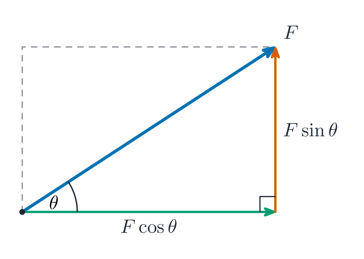
A force at angle $\theta$ has a horizontal part $F\cos\theta$ and a vertical part $F\sin\theta$. A particle is in equilibrium 平衡 when the forces are balanced: the vector sum of the forces is zero. In practice this means the components in any direction add to zero.

Every mechanics problem is a picture like this. Three forces act on the climber — weight straight down, tension along the rope, and a push from the rock — and because they balance, the climber hangs still in equilibrium. Resolving each into horizontal and vertical parts turns the picture into equations Friction
When two surfaces touch, the contact force 接触力 between them has two parts: the normal reaction 法向反作用力 $R$, at right angles to the surface, and the friction 摩擦力 $F$, along the surface, which opposes sliding. A "smooth" surface is a model with no friction.
Friction can only grow up to a maximum. At that maximum the body is in limiting equilibrium 极限平衡, about to slip, and the friction is limiting friction 最大静摩擦力. The maximum is set by the coefficient of friction 摩擦系数 $\mu$:
$$F \leqslant \mu R, \qquad \text{with } F = \mu R \text{ at the point of slipping}.$$
On a rough surface the contact force splits into the normal reaction $R$ and friction $F$ (at most $\mu R$). By Newton's third law 牛顿第三定律, the two surfaces push on each other with equal and opposite forces.
Worked example. A block of weight $20\text{ N}$ rests on a rough horizontal table with coefficient of friction $\mu = 0.4$. Find the largest horizontal force that can be applied before the block slides.
The table's normal reaction balances the weight, so $R = 20\text{ N}$. The block is on the point of slipping when friction reaches its maximum $F = \mu R = 0.4 \times 20 = 8\text{ N}$. In equilibrium the applied force equals the friction, so the largest force it can resist is $8\text{ N}$.
탐색하기힘의 합성
합력 = a + b
힘은 끝머리-시작머리로 합해집니다. 합력이 0이면 평형 상태입니다.
어휘 연습하기English 한국어 Mechanics/mɪˈkænɪks/ Mechanics force/fɔːs/ force components/kəmˈpəʊnənts/ components resultant/rɪˈzʌltənt/ resultant equilibrium/ˌiːkwɪˈlɪbrɪəm/ equilibrium contact force/ˈkɒntækt fɔːs/ contact force normal reaction/ˈnɔːml rɪˈækʃn/ normal reaction friction/ˈfrɪkʃn/ friction limiting friction/ˈlɪmɪtɪŋ ˈfrɪkʃn/ limiting friction coefficient of friction/ˌkəʊɪˈfɪʃənt ɒv ˈfrɪkʃn/ coefficient of friction Newton's third law/ˈnjuːtnz θɜːd lɔː/ Newton's third law limiting equilibrium/ˈlɪmɪtɪŋ ˌiːkwɪˈlɪbrɪəm/ limiting equilibrium 4.2
Kinematics of motion in a straight line

Syllabus
지원자는 다음을 할 수 있어야 한다: 참고 사항 및 예시 거리와 속력이 스칼라량이며, 변위, 속도 및 가속도가 벡터량임을 이해함 1차원 운동에만 제한됨. '감속'이라는 용어가 occasionally 속력의 감소를 나타내는 맥락에서 사용될 수 있음. 변위-시간 그래프와 속도-시간 그래프를 그리며 해석하고, 특히 – 속도-시간 그래프 아래 면적이 변위를 나타냄, – 변위-시간 그래프의 기울기가 속도를 나타냄, – 속도-시간 그래프의 기울기가 가속도를 나타냄 –을 인식함 미분 및 적분을 시간의 함수로 사용하여 변위, 속도 및 가속도와 관련된 간단한 문제를 풀기 필요한 미적분 기법은 Paper 1: 순수 수학 1의 내용에 제한됨. 직선运动中 일정한 가속도를 가진 운동에 대한 적절한 공식 사용. 여러 입자의 운동에 대한 정보를 사용하여 하나의 방정식보다 많은 방정식을 세우는 문제가 포함될 수 있음. 출처: Cambridge International syllabus
Distance 距离 and speed 速率 are scalars (size only). Displacement 位移, velocity 速度 and acceleration 加速度 are vectors (size and direction).
On a velocity-time graph 速度时间图, the area under the graph is the displacement and the gradient is the acceleration (a negative acceleration is a deceleration 减速度). On a displacement-time graph, the gradient is the velocity. More generally, differentiate with respect to time to go from displacement to velocity to acceleration, and integrate to go back.
The shaded area gives the distance travelled; the slope of the line gives the acceleration. For motion with constant acceleration 匀加速, use these formulae (the "suvat" equations):
$$v = u + at, \qquad s = ut + \tfrac12 at^2, \qquad v^2 = u^2 + 2as, \qquad s = \tfrac12(u + v)t.$$Worked example. A car starts from rest and accelerates at $2.5\ \text{m s}^{-2}$ for $4\ \text{s}$. Find its speed and the distance travelled.
$$v = 0 + 2.5\times 4 = 10\ \text{m s}^{-1}, \qquad s = 0 + \tfrac12(2.5)(4^2) = 20\ \text{m}.$$탐색하기속도-시간 그래프
초기 속도와 가속도를 변경하세요. 기울기는 가속도이며, 선 아래의 면적은 변위(displacement)입니다.
어휘 연습하기English 한국어 distance/ˈdɪstəns/ distance speed/spiːd/ speed displacement/dɪˈspleɪsmənt/ displacement velocity/vəˈlɒsɪti/ velocity acceleration/əkˌseləˈreɪʃn/ acceleration velocity-time graph/vəˈlɒsɪti taɪm ɡræf/ velocity-time graph constant acceleration/ˈkɒnstənt əkˌseləˈreɪʃn/ constant acceleration deceleration/dɪˌseləˈreɪʃn/ deceleration 4.3
Momentum

Syllabus
지원자는 다음을 할 수 있어야 한다: 참고 사항 및 예시 선운동량의 정의를 사용하고, 그 벡터적 성질을 보여줌 1차원 운동에만 제한됨. 선운동량의 보존 법칙을 사용하여 두 물체의 정면 충돌로 모델링될 수 있는 문제를 풀기 두 물체가 충돌 시 결합되는 정면 충돌을 포함함. 임펄스와 반발 계수에 대한 지식은 불필요함. 출처: Cambridge International syllabus
A Newton's cradle demonstrates conservation of momentum in collisions. The linear momentum 动量 of a body is $\text{mass} \times \text{velocity}$. It is a vector. In a direct collision of two bodies, the total momentum is unchanged. This is the conservation of linear momentum 动量守恒:
$$m_1 u_1 + m_2 u_2 = m_1 v_1 + m_2 v_2.$$
The total momentum is the same before and after the collision. Worked example. A body of mass $2\ \text{kg}$ moving at $3\ \text{m s}^{-1}$ hits a stationary body of mass $1\ \text{kg}$, and they stick together. Find their common speed afterwards.
$$2(3) + 1(0) = (2 + 1)v \;\Rightarrow\; v = \frac{6}{3} = 2\ \text{m s}^{-1}.$$탐색하기충돌
각 질량과 속도를 설정하고 충돌시킵니다. 충돌 전후로 전체 운동량은 동일하게 유지됩니다.
어휘 연습하기English 한국어 momentum/məʊˈmentəm/ momentum conservation of momentum/ˌkɒnsəˈveɪʃn ɒv məʊˈmentəm/ conservation of momentum 4.4
Newton's laws of motion

Syllabus
Candidates should be able to: Notes and examples • apply Newton’s laws of motion to the linear motion of a particle of constant mass moving under the action of constant forces, which may include friction, tension in an inextensible string and thrust in a connecting rod If any other forces resisting motion are to be considered (e.g. air resistance) this will be indicated in the question. • use the relationship between mass and weight $W = mg$. In this component, questions are mainly numerical, and use of the approximate numerical value $10\text{ (ms}^{-2}\text{)}$ for $g$ is expected. • solve simple problems which may be modelled as the motion of a particle moving vertically or on an inclined plane with constant acceleration Including, for example, motion of a particle on a rough plane where the acceleration while moving up the plane is different from the acceleration while moving down the plane. • solve simple problems which may be modelled as the motion of connected particles. e.g. particles connected by a light inextensible string passing over a smooth pulley, or a car towing a trailer by means of either a light rope or a light rigid tow-bar. 출처: Cambridge International syllabus
Newton's laws of motion 牛顿运动定律 connect force and acceleration. The key one is: resultant force $=$ mass 质量 $\times$ acceleration,
$$F = ma.$$The weight 重力 of a body is the force of gravity on it: $W = mg$. Forces in a problem may include weight, friction, tension 张力 in a string, the thrust 推力 (push) in a rod, and air resistance 空气阻力.For motion on an inclined plane 斜面, split each force into a part along the slope and a part at right angles to it, then apply $F = ma$ along the slope. For connected particles 连接质点 (joined by a string), apply $F = ma$ to each body, or to the whole system.
On a slope, resolve the forces along the slope and at right angles to it. Worked example. A block of mass $12\ \text{kg}$ is pulled up a rough plane by a rope parallel to the slope. The plane is at $20^\circ$ to the horizontal, the coefficient of friction is $0.4$, and the acceleration is $2\ \text{m s}^{-2}$. Find the tension in the rope.
The normal reaction is $R = mg\cos 20^\circ = 120\cos 20^\circ = 112.8\ \text{N}$, so the friction is $F = \mu R = 0.4 \times 112.8 = 45.1\ \text{N}$. Along the slope, $T - mg\sin 20^\circ - F = ma$:
$$T = ma + mg\sin 20^\circ + F = 12(2) + 120\sin 20^\circ + 45.1 = 24 + 41.0 + 45.1 = 110\ \text{N (3 s.f.)}.$$탐색하기합력
F = ma
합력이 가속도를 결정한다. 균형 잡힌 힘 ⇒ 가속도 없음.
어휘 연습하기English 한국어 Newton's laws of motion/ˈnjuːtnz lɔːz ɒv ˈməʊʃn/ Newton's laws of motion mass/mæs/ mass weight/weɪt/ weight tension/ˈtenʃn/ tension inclined plane/ɪnˈklaɪnd pleɪn/ inclined plane connected particles/kəˈnektɪd ˈpɑːtɪklz/ connected particles thrust/θrʌst/ thrust air resistance/eə rɪˈzɪstəns/ air resistance 4.5
Energy, work and power

Syllabus
지원자는 다음을 할 수 있어야 한다: 참고 사항 및 예시 • 힘에 의해 된 일의 개념을 이해하고, 점의 적용점이 힘과 평행하지 않은 변위를 할 때 상수 힘에 의해 된 일을 계산함 $W = Fd \cos \theta$; 스칼라 곱의 사용은 불필요함. • 중력ポテンシャル 에너지와 운동 에너지의 개념을 이해하고 적절한 공식 사용 • 시스템의 에너지 변화와 외부력에 의해 된 일 사이의 관계를 이해하고 사용하며, appropriate한 경우 에너지 보존의 법칙 사용 운동이 선형일 수 없는 경우(예: 매끄러운 곡선 '슬라이드' 위의 아이)를 포함하며, 전체 에너지 변화만 고려하면 됨. • 출력이 힘에 의해 일을 하는 비율임을 정의하고, 운동 방향에 작용하는 힘에 대한 출력, 힘 및 속도 사이의 관계 사용 (평균) 출력 계산 $$\frac{\text{Work done}}{\text{Time taken}}$$$P = Fv$을 포함함.예를 들어, 경사면을 오르는 차가 저항을 이겨서 순간 가속도를 구하는 문제 풀이. 출처: Cambridge International syllabus
A roller coaster trades potential energy for kinetic energy as it rises and falls. The work done 功 by a constant force is the scalar product of force and displacement — the force times the distance moved in the direction of the force: $W = Fd\cos\theta$, where $\theta$ is the angle between the force and the motion. Work is measured in joules (J).
Energy comes in forms you can calculate:
- Kinetic energy 动能 (energy of movement): $\text{KE} = \tfrac12 mv^2$.
- Gravitational potential energy 重力势能 (energy of height): $\text{PE} = mgh$.
The work done by the outside forces equals the change in the total energy. When no friction acts, the total energy stays the same — the conservation of energy 能量守恒.
Power 功率 is the rate of doing work. For a force pulling in the direction of motion, $P = Fv$ (power $=$ force $\times$ velocity). Power is measured in watts (W).
Worked example. A car engine works at $12\ \text{kW}$ while the car moves at $20\ \text{m s}^{-1}$ on a level road. Find the driving force.
$$P = Fv \;\Rightarrow\; F = \frac{P}{v} = \frac{12000}{20} = 600\ \text{N}.$$탐색하기에너지 보존
물체를 떨어뜨리고 에너지가 어떻게 변환되는지 관찰하세요. 마찰이 없는 경우, 중력 위치에너지(GPE) + 운동에너지(KE)가 전체 하강 과정 동안 일정하게 유지됩니다.
어휘 연습하기English 한국어 work done/wɜːk dʌn/ work done kinetic energy/kɪˈnetɪk ˈenədʒi/ kinetic energy gravitational potential energy/ˌɡrævɪˈteɪʃənl pəˈtenʃl ˈenədʒi/ gravitational potential energy conservation of energy/ˌkɒnsəˈveɪʃn ɒv ˈenədʒi/ conservation of energy power/ˈpaʊə/ power 4.5
Exam tips
- Draw a clear force diagram and resolve into perpendicular components; for equilibrium, each direction sums to zero.
- Use SUVAT only for constant acceleration and keep a consistent positive direction.
- Apply $F = ma$ along the direction of motion, including friction ($F = \mu R$) on a rough surface.
- State your assumptions (light inextensible string, smooth pulley, particle) — they are often worth a mark.
-
5
확률 및 통계 1
수업 보기This handout covers Topic 5: Probability & Statistics 概率统计 1. It is about describing data, counting choices, and working out the chance of events.
5.1
Representation of data

Syllabus
지원자는 다음을 할 수 있어야 한다: 참고 사항 및 예시 • 원시 통계 데이터를 제시하는 적절한 방법을 선택하고, 특정 표현 방식의 장점과/또는 단점을 논의함 스テム 앤 리프 다이어그램, 상자 수염 plot, 히스토그램 및 누적 빈도 그래프를 그리며 해석함 백 투 백 스템 앤 리프 다이어그램 포함. 중앙 경향(평균, 중앙값, 최빈값) 및 변동(범위, 사분위 범위, 표준 편차)의 다양한 측정方法来 이해하고 사용함 예를 들어, 데이터셋을 비교 및 대비할 때. • 누적 빈도 그래프를 사용하여 예: 중앙값, 사분위수, 백분위수를 추정하거나, 주어진 값보다 위(또는 아래)에 있는 분포의 비율 또는 두 값 사이의 비율을 구하는 데 활용. • 데이터 자체에서 주어진 합계 $\Sigma x$ 및 $\Sigma x^2$, 또는 부호화된 합계 $\Sigma(x - a)$ 및 $\Sigma(x - a)^2$로부터 평균과 표준편차를 계산하고 사용함(구분된 데이터 포함). 이러한 합계를 이용하여 최대 2개의 데이터 세트를 포함할 수 있는 문제 해결에 적용. 출처: Cambridge International syllabus
Choose a diagram that suits the data. You should be able to draw and read:
- a stem-and-leaf diagram 茎叶图 (keeps the original values and shows the shape); two data sets are compared with a back-to-back 背靠背 version – a shared central stem, one set's leaves increasing to the left and the other's to the right, so you can compare their medians and spreads at a glance;
- a box-and-whisker plot 箱线图 (shows the lowest value, the three quartiles, and the highest value);
- a histogram 直方图 (for grouped data, where the area of each bar shows the frequency);
- a cumulative frequency 累积频数 graph (running totals, used to estimate the median and quartiles).
A cumulative frequency curve is S-shaped; read the median across from half the total frequency, and the quartiles from one and three quarters 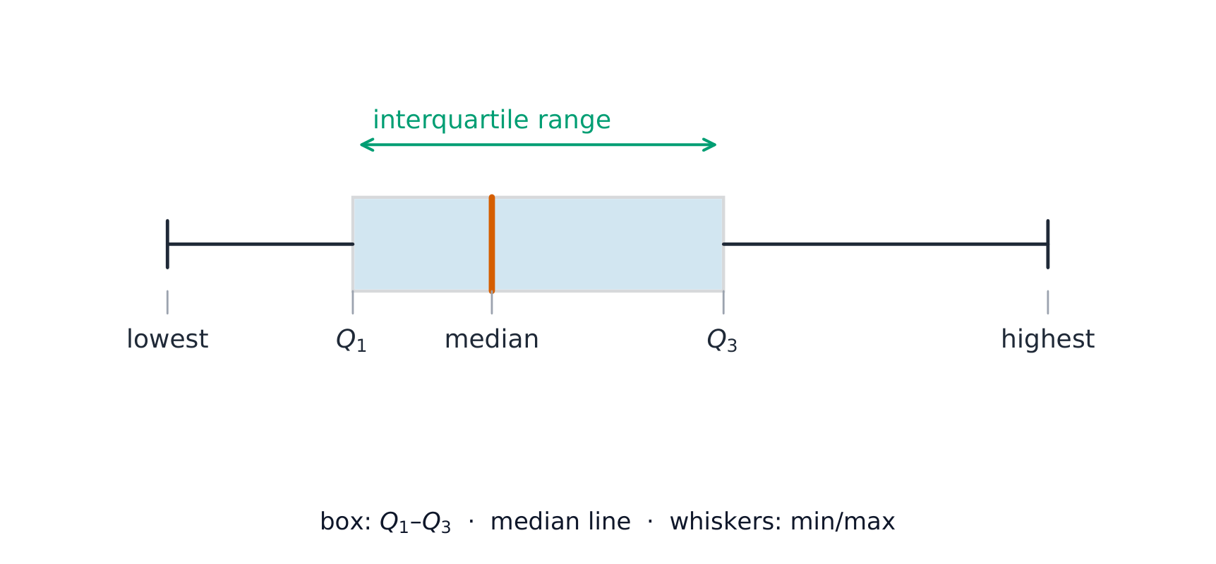
The box spans the quartiles $Q_1$ to $Q_3$; the whiskers reach the lowest and highest values. Averages and spread
A measure of central tendency 集中趋势 is a single "middle" value:
- the mean 平均数 $\bar{x} = \dfrac{\sum x}{n}$ (the average);
- the median 中位数 (the middle value when the data is in order);
- the mode 众数 (the most common value).
A measure of variation 离散程度 shows how spread out the data is:
- the range (of data) 极差 (highest $-$ lowest);
- the interquartile range 四分位距 (upper quartile $-$ lower quartile);
- the standard deviation 标准差 $\sigma = \sqrt{\dfrac{\sum x^2}{n} - \bar{x}^2}$.
You often work from the totals $\sum x$ and $\sum x^2$. The square of the standard deviation is the variance 方差.
Worked example. For $10$ values, $\sum x = 50$ and $\sum x^2 = 300$. Find the mean and standard deviation.
$$\bar{x} = \frac{50}{10} = 5, \qquad \sigma = \sqrt{\frac{300}{10} - 5^2} = \sqrt{30 - 25} = \sqrt{5} = 2.24.$$Coding 编码 makes big numbers easier. Replace each value by $t=x-a$ for a convenient assumed mean 假定平均数 $a$. Then $\bar{x}=a+\bar{t}$, while the standard deviation is unchanged (shifting every value does not spread the data). So from the coded totals $\sum(x-a)$ and $\sum(x-a)^2$ you get $\bar x$ and $\sigma$ directly, and two data sets can be compared through their coded totals.
탐색하기산포와 종 모양
P(−k < Z < k)
산포는 표준편차로 측정된다 — 데이터의 약 68%는 1 sd 이내, 95%는 2 sd 이내에 존재한다.
어휘 연습하기English 한국어 stem-and-leaf diagram/stem ænd liːf ˈdaɪəɡræm/ 줄기와 잎 도표(stem-and-leaf diagram) back-to-back/bæk tə bæk/ 등반 도표(back-to-back) box-and-whisker plot/bɒks ænd ˈwɪskə plɒt/ 상자 수염 그림(box-and-whisker plot) histogram/ˈhɪstəɡræm/ 히스토그램 cumulative frequency/ˈkjuːmjʊlətɪv ˈfriːkwənsi/ 누적 빈도 measure of central tendency/ˈmeʒə ɒv ˈsentrəl ˈtendənsi/ 집중 경향의 측정 mean/miːn/ 평균 median/ˈmiːdiːən/ 중位数Unless median. mode/məʊd/ 최빈값 variation/ˌveərɪˈeɪʃn/ 변화 range (of data)/reɪndʒ/ 범위 (데이터) interquartile range/ˌɪntəˈkwɔːtaɪl reɪndʒ/ 사분위 범위 standard deviation/ˈstændəd ˌdiːvɪˈeɪʃn/ 표준편차 variance/ˈveərɪəns/ 편차 Coding/ˈkəʊdɪŋ/ 코딩 assumed mean/əˈsjuːmd miːn/ 가정 평균 central tendency/ˈsentrəl ˈtendənsi/ 집중 경향 5.2
Permutations and combinations

Syllabus
지원자는 다음을 할 수 있어야 한다: 참고 사항 및 예시 • 순열(permutation) 과 조합(comination) 의 개념을 이해하고, 선택과 관련된 간단한 문제를 해결함 • 줄에 배치되는 물체의 배열에 관한 문제를 해결함. 반복이 포함된 경우(예: ‘NEEDLESS’라는 단어의 문자를 나열하는 방법의 수) 및 제한 조건이 있는 경우(예: 특정 2명이 반드시 옆에 서야 하거나, 옆에 서지 말아야 할 때 여러 사람이 줄을 서는 방법의 수)를 포함. 질문에는 사람들이 두 개(또는 그 이상)의 행에 앉아 있는 경우가 포함될 수 있음. 원형으로 배열되는 물체에 대한 질문은 포함되지 않음. 출처: Cambridge International syllabus
A permutation 排列 is an arrangement where order matters; a combination 组合 is a selection where order does not matter. The numbers are
$${}^nP_r = \frac{n!}{(n-r)!}, \qquad {}^nC_r = \binom{n}{r} = \frac{n!}{r!\,(n-r)!}.$$To arrange objects in a line when some are repeated, divide by the factorial of each repeat count.Order matters for a permutation, but not for a combination Worked example. How many different arrangements are there of the letters of the word NEEDLESS?
There are $8$ letters, with E repeated $3$ times and S repeated $2$ times:
$$\frac{8!}{3!\,2!} = \frac{40320}{6 \times 2} = 3360.$$
nPr = n!/(n−r)!; nCr = nPr/r! 탐색하기순열 또는 조합 실험실
세는 문제에서 순서가 중요한지 선택하십시오.
어휘 연습하기English 한국어 permutation/ˌpɜːmjuːˈteɪʃn/ 배열 combination/ˌkɒmbɪˈneɪʃn/ 조합 5.3
Probability

Syllabus
지원자는 다음을 할 수 있어야 한다: 참고 사항 및 예시 등확률 기본 사건을 열거하거나, 순열 또는 조합을 사용하여 계산함으로써 간단한 경우의 확률을 평가함 예: 공정한 주사위를 두 개 던졌을 때 총점. 예: 서로 다른 색상의 공이 들어있는 주머니에서 무작위로 공을 꺼내는 경우. 적절한 경우에 확률의 덧셈과 곱셈 법칙을 사용함 일반 공식 $\text{P}(A \cup B) = \text{P}(A) + \text{P}(B) - \text{P}(A \cap B)$의 명시적 사용은 필요하지 않음. 상호 배타적(exclusive) 과 독립(independent) 사건의 의미를 이해하며, 사건 $A$와 $B$가 독립인지 여부를 $\text{P}(A \cap B)$과 $\text{P}(A) \times \text{P}(B)$의 값을 비교하여 판단함 간단한 경우의 조건부 확률을 계산하고 사용함. 예: 등확률 기본 사건의 표본 공간이나 나무 도도로 표현 가능한 상황. 간단한 경우 $\text{P}(A|B) = \frac{\text{P}(A \cap B)}{\text{P}(B)}$의 사용이 필요할 수 있음. 출처: Cambridge International syllabus
Dice: a familiar starting point for probability. Find a probability by counting equally likely outcomes, or by using permutations and combinations. Combine probabilities with these rules:
- addition for "or": $P(A \cup B) = P(A) + P(B) - P(A \cap B)$;
- multiplication for "and" when events are independent: $P(A \cap B) = P(A)\,P(B)$.

The overlap of the two circles is $A\cap B$; the addition rule subtracts it once so it is not counted twice. Two events are mutually exclusive events 互斥事件 if they cannot both happen, and independent events 独立事件 if one happening does not change the chance of the other. To test independence, check whether $P(A \cap B) = P(A)\times P(B)$. A conditional probability 条件概率 is the chance of $A$ given that $B$ has happened: $P(A \mid B) = \dfrac{P(A \cap B)}{P(B)}$.
Worked example. Events have $P(A) = 0.5$, $P(B) = 0.4$ and $P(A \cap B) = 0.2$. Are $A$ and $B$ independent?
Test: $P(A)\times P(B) = 0.5 \times 0.4 = 0.2 = P(A \cap B)$. The values are equal, so $A$ and $B$ are independent.
탐색하기조건부 확률
확률값을 변경하여 나무 도표(tree) 를 읽어보세요. P(A and B)와 조건부 확률이 어떻게 결합되는지 보여주는 방법입니다.
어휘 연습하기English 한국어 mutually exclusive events/ˈmjuːtʃuːəli eksˈkluːsɪv ɪˈvents/ 상호 배타적 사건 independent events/ˌɪndɪˈpendənt ɪˈvents/ 독립 사건 conditional probability/kənˈdɪʃənl ˌprɒbəˈbɪlɪti/ 조건부 확률 5.4
Discrete random variables
Syllabus
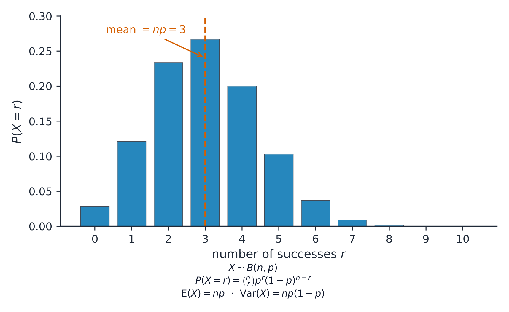
지원자는 다음을 할 수 있어야 한다: 참고 사항 및 예시 이산 확률변수 $X$와 관련된 주어진 상황에 대해 확률 분포 표를 작성하고, $\text{E}(X)$ 및 $\text{Var}(X)$를 계산함 이항 분포와 기하 분포에 대한 확률 공식을 사용하고, 이러한 분포가 적절한 모델로 사용될 수 있는 실제 상황을 식별함 기호 $\text{B}(n, p)$ 및 $\text{Geo}(p)$ 포함. $\text{Geo}(p)$는 $p_r = p(1 - p)^{r-1}$가 $r = 1, 2, 3, \dots$인 분포를 나타냄. 이항 분포의 기대치와 분산 공식 및 기하 분포의 기대치 공식을 사용함. 공식의 증명은 필요하지 않음. 출처: Cambridge International syllabus
A discrete random variable 离散型随机变量 $X$ takes separate values, each with a probability. List them in a probability distribution table 概率分布表; the probabilities must add to $1$. Then the expectation 期望 (mean) and variance are
$$E(X) = \sum x\,P(X = x), \qquad \mathrm{Var}(X) = \sum x^2\,P(X = x) - \big(E(X)\big)^2.$$Two special models:
- the binomial distribution 二项分布 $X \sim B(n, p)$, for the number of successes in $n$ independent trials: $P(X = r) = \binom{n}{r}p^r(1-p)^{n-r}$, with $E(X) = np$ and $\mathrm{Var}(X) = np(1-p)$;
- the geometric distribution 几何分布, for the trial on which the first success happens: $P(X = r) = (1-p)^{r-1}p$, with $E(X) = \dfrac{1}{p}$.
Worked example. $X \sim B(10, 0.3)$. Find $P(X = 2)$ and $E(X)$.
$$P(X = 2) = \binom{10}{2}(0.3)^2(0.7)^8 = 45 \times 0.09 \times 0.05765 = 0.233, \qquad E(X) = 10 \times 0.3 = 3.$$The distribution $B(10,0.3)$: each bar is $P(X=r)$, clustered around the mean $np=3$. 탐색하기이산 분포 discrete distribution
이항 분포(binomial) 의 n과 p를 변경하여 막대를 확인하세요. 각 성공 횟수의 확률입니다.
어휘 연습하기English 한국어 discrete random variable/dɪˈskriːt ˈrændəm ˈveərɪəbl/ 이산 확률 변수 probability distribution table/ˌprɒbəˈbɪlɪti ˌdɪstrɪˈbjuːʃn ˈteɪbl/ 확률 분포표 expectation/ekspɪkˈteɪʃn/ 기대값 binomial distribution/baɪˈnəʊmɪəl ˌdɪstrɪˈbjuːʃn/ 이항분포 geometric distribution/ˌdʒiːəʊˈmetrɪk ˌdɪstrɪˈbjuːʃn/ 기하 분포 5.5
The normal distribution

Syllabus
Candidates should be able to: Notes and examples understand the use of a normal distribution to model a continuous random variable, and use normal distribution tables Sketches of normal curves to illustrate distributions or probabilities may be required. solve problems concerning a variable $X$, where $X \sim N(\mu, \sigma^2)$, including: – finding the value of $P(X > x_1)$, or a related probability, given the values of $x_1$, $\mu$, $\sigma$. – finding a relationship between $x_1$, $\mu$ and $\sigma$ given the value of $P(X > x_1)$ or a related probability For calculations involving standardisation, full details of the working should be shown. e.g. $Z = \frac{(X - \mu)}{\sigma}$ recall conditions under which the normal distribution can be used as an approximation to the binomial distribution, and use this approximation, with a continuity correction, in solving problems. $n$ sufficiently large to ensure that both $np > 5$ and $nq > 5$. 출처: Cambridge International syllabus
The 68-95-99.7 rule A Galton board: balls falling through pins pile up into the bell-shaped normal distribution. The normal distribution 正态分布 models a continuous random variable 连续型随机变量 with a symmetric bell shape. Write $X \sim N(\mu, \sigma^2)$, where $\mu$ is the mean and $\sigma$ is the standard deviation. To use the tables, by standardisation 标准化 convert to the variable $Z \sim N(0, 1)$:
$$Z = \frac{X - \mu}{\sigma}.$$Then $P(X < x) = P\!\left(Z < \dfrac{x - \mu}{\sigma}\right)$, which you read from the normal table $\Phi$.

A normal probability is an area under the bell curve; standardizing rescales it to $Z\sim N(0,1)$. The normal distribution is also a good approximation 近似 to the binomial when $n$ is large. Because you replace a discrete variable by a continuous one, apply a continuity correction 连续性校正 (adjust by $0.5$).
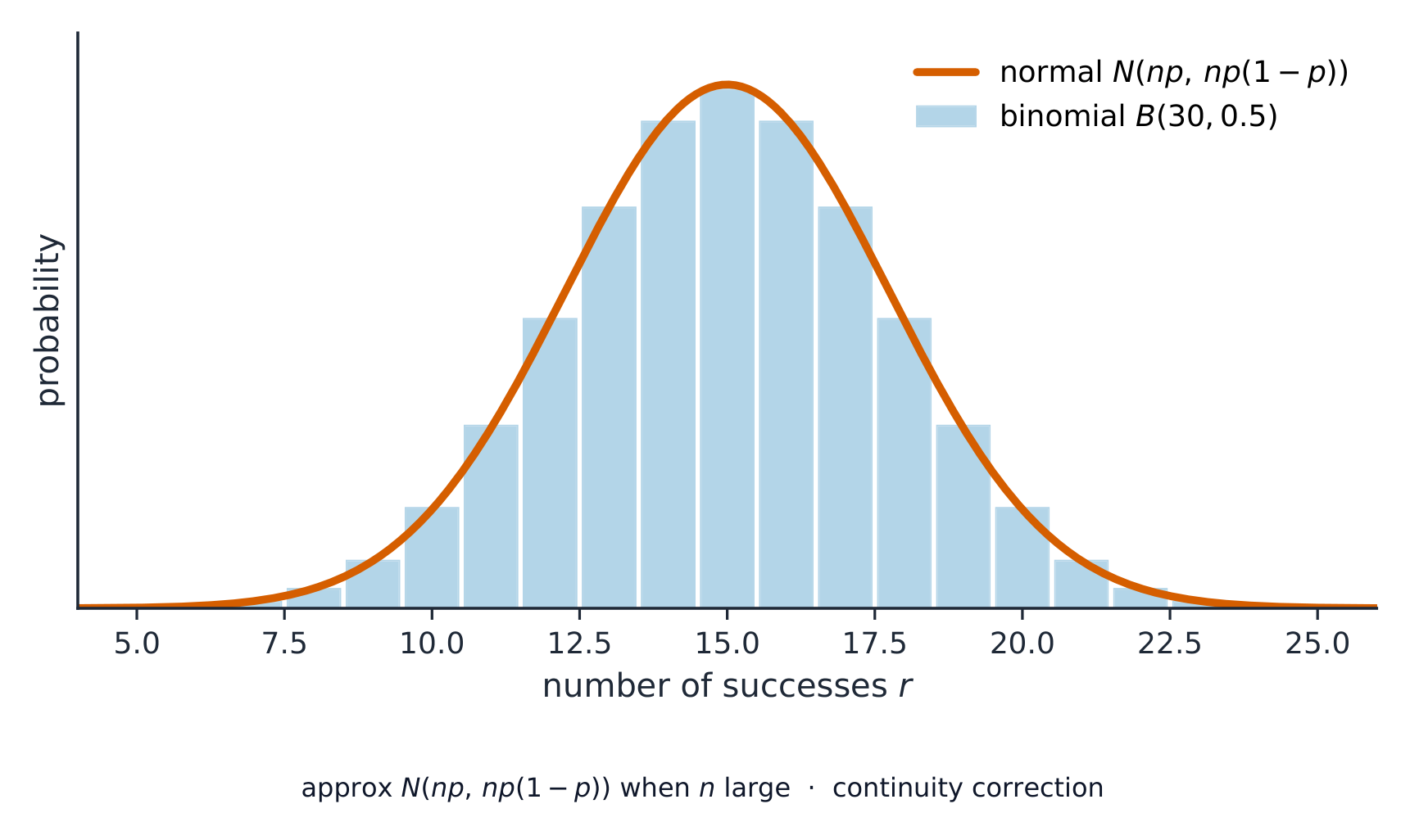
When $n$ is large the binomial bars follow a normal curve of the same mean and variance. Worked example. Bags of rice have mass $X \sim N(\mu, 0.14^2)$. Given that $P(X < 1.48) = 0.22$, find $\mu$.
From the table, $P(Z < z) = 0.22$ gives $z = -0.772$. So
$$\frac{1.48 - \mu}{0.14} = -0.772 \;\Rightarrow\; \mu = 1.48 + 0.772 \times 0.14 = 1.59\ \text{kg (3 s.f.)}.$$탐색하기정규 분포
영역을 채워 확률을 구하세요. z-value(z점수) 는 점이 평균으로부터 표준편차 몇 개만큼 떨어져 있는지를 측정합니다.
어휘 연습하기English 한국어 normal distribution/ˈnɔːml ˌdɪstrɪˈbjuːʃn/ 표준정규분포 continuous random variable/kənˈtɪnjuːəs ˈrændəm ˈveərɪəbl/ 연속 확률 변수 standardisation/ˌstændədaɪˈzeɪʃn/ 표준화 approximation/əˌprɒksɪˈmeɪʃn/ 근사(approximation) continuity correction/kɒntɪˈnjuːɪti kəˈrekʃn/ 연속성 보정 Probability & Statistics/ˌprɒbəˈbɪlɪti ænd stəˈtɪstɪks/ 확률 및 통계 5.5
Exam tips
- Decide whether order matters: permutations ($^nP_r$) when it does, combinations ($^nC_r$) when it does not.
- For a discrete random variable, check the probabilities sum to $1$ and use $E(X) = \sum x\,P(X=x)$.
- For the normal distribution, standardise with $z = (x - \mu)/\sigma$, sketch and shade, then read the table.
- Apply a continuity correction when approximating a discrete variable by the normal.
-
6
확률 및 통계 2
수업 보기This handout covers Topic 6: Probability & Statistics 概率统计 2. It adds the Poisson model, combining random variables, continuous distributions, and the ideas of estimation and testing.
6.1
The Poisson distribution

Syllabus
지원자는 다음을 할 수 있어야 한다: 참고 사항 및 예시 공식을 사용하여 분포 $\text{Po}(\lambda)$에 대한 확률을 계산한다. • $X \sim \text{Po}(\lambda)$일 때 $X$의 평균과 분산이 각각 $\lambda$와 같다는 사실을 사용함 증명은 필요하지 않음. • 포아송 분포가 무작위 사건의 분포와 관련이 있음을 이해하고, 포아송 분포를 모델로 사용함 • 적절한 경우 포아송 분포를 이항 분포의 근사로 사용함 $n$가 크고 $p$이 작아야 한다는 조건을 알고 있어야 함; $n > 50$와 $np < 5$는 대략적으로. • 적절한 경우 포아송 분포의 근사로 연속성 보정을 포함하는 정규 분포를 사용함. $\lambda$가 크어야 한다는 조건을 알고 있어야 함; $\lambda > 15$는 대략적으로. 출처: Cambridge International syllabus
People arriving at random in a queue follow a Poisson distribution. The Poisson distribution 泊松分布 $X \sim \mathrm{Po}(\lambda)$ models the number of random events in a fixed interval, when events happen at a steady average rate $\lambda$:
$$P(X = r) = e^{-\lambda}\frac{\lambda^r}{r!}.$$For a Poisson variable the mean and the variance are both equal to $\lambda$. The Poisson distribution is a good approximation 近似 to the binomial distribution when $n$ is large and $p$ is small. The normal distribution (with continuity correction) approximates the Poisson when $\lambda$ is large.Worked example. $X \sim \mathrm{Po}(3)$. Find $P(X = 2)$.
$$P(X = 2) = e^{-3}\frac{3^2}{2!} = e^{-3}\times 4.5 = 0.224.$$
The Poisson distribution $\mathrm{Po}(3)$: for a Poisson variable the mean and variance both equal $\lambda$. 탐색하기포아송 분포
평균 λ를 변경하세요. 포아송 분포는 고정된 구간 내 무작위 사건(random events) 의 개수를 모델링하며, 드문 사건은 왜곡된 형태를 가집니다.
어휘 연습하기English 한국어 Poisson distribution/ˈpɔɪsn ˌdɪstrɪˈbjuːʃn/ 푸아송 분포 approximation/əˌprɒksɪˈmeɪʃn/ 근사(approximation) 6.2
Linear combinations of random variables
Syllabus
지원자는 다음을 할 수 있어야 한다: 참고 사항 및 예시 • 문제 해결 시 다음 결과를 사용함 – $\text{E}(aX + b) = a\text{E}(X) + b$ 및 $\text{Var}(aX + b) = a^2\text{Var}(X)$ – $\text{E}(aX + bY) = a\text{E}(X) + b\text{E}(Y)$ – $\text{Var}(aX + bY) = a^2\text{Var}(X) + b^2\text{Var}(Y)$는 독립인 $X$ 및 $Y$에 대해 – $X$가 정규 분포를 가지면 $aX + b$도 정규 분포를 가짐 – $X$와 $Y$가 독립적인 정규 분포를 가지면 $aX + bY$가 정규 분포를 가짐 – $X$과 $Y$가 독립적인 포아송 분포를 가지면 $X + Y$이 포아송 분포를 가짐. 이 결과들의 증명은 필요하지 않음. 출처: Cambridge International syllabus
When you change a variable by a linear rule, the expectation 期望 (mean) and variance 方差 follow these rules:
$$E(aX + b) = aE(X) + b, \qquad \mathrm{Var}(aX + b) = a^2\,\mathrm{Var}(X).$$For two independent variables $X$ and $Y$:$$E(aX + bY) = aE(X) + bE(Y), \qquad \mathrm{Var}(aX + bY) = a^2\,\mathrm{Var}(X) + b^2\,\mathrm{Var}(Y).$$Two useful facts: if $X$ has a normal distribution 正态分布 then so does $aX + b$; and the sum of independent Poisson variables is again Poisson.Worked example. $X$ has mean $5$ and variance $4$. Find $E(3X - 1)$ and $\mathrm{Var}(3X - 1)$.
$$E(3X - 1) = 3(5) - 1 = 14, \qquad \mathrm{Var}(3X - 1) = 3^2 \times 4 = 36.$$탐색하기선형 결합 실험실
E(aX + b) = aE(X) + b
스케일링 인자를 변경하여 기대값이 어떻게 변화하는지 확인하시오.
어휘 연습하기English 한국어 expectation/ekspɪkˈteɪʃn/ 기대값 variance/ˈveərɪəns/ 편차 normal distribution/ˈnɔːml ˌdɪstrɪˈbjuːʃn/ 표준정규분포 6.3
Continuous random variables
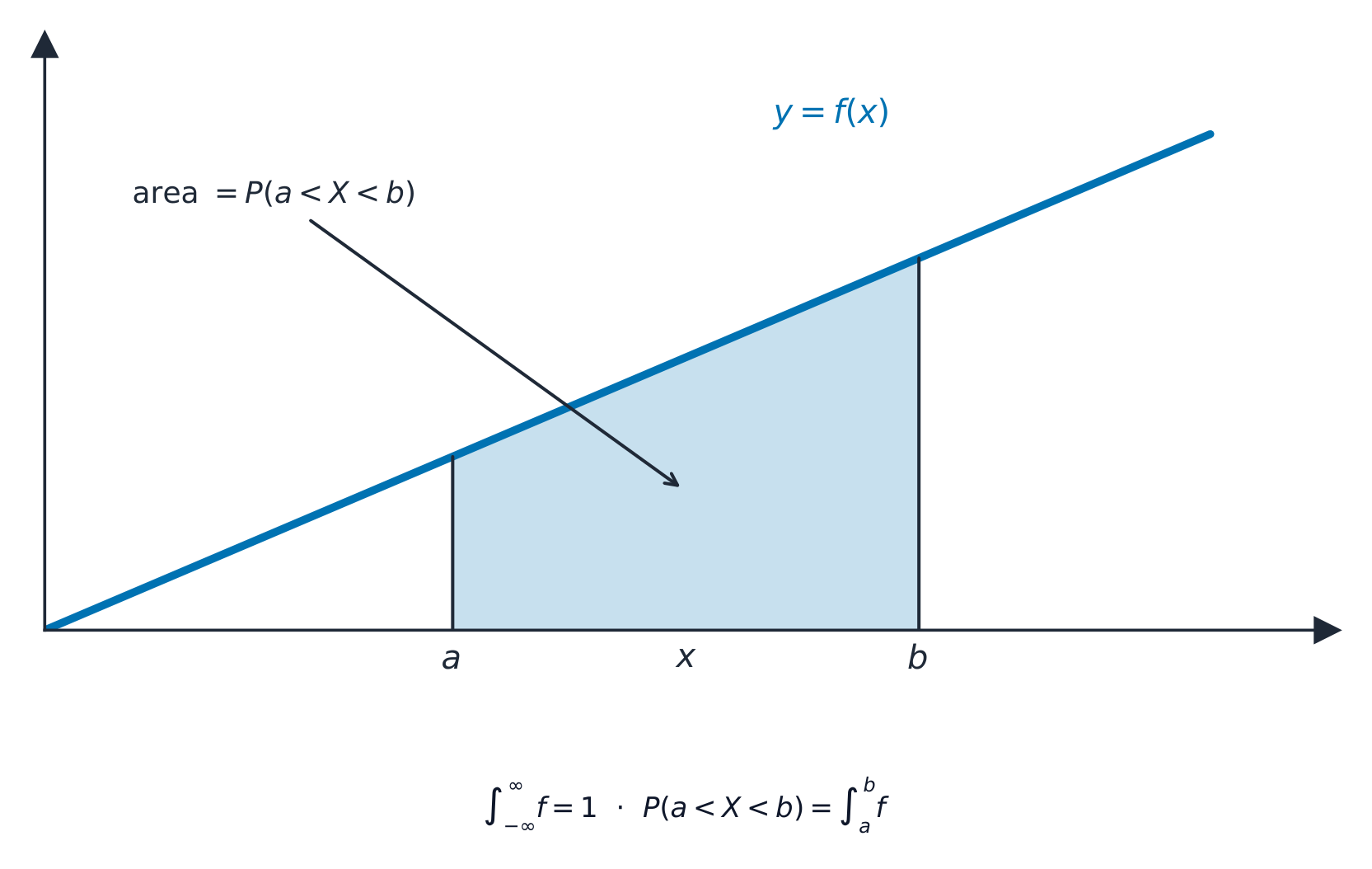
Syllabus
지원자는 다음을 할 수 있어야 한다: 참고 사항 및 예시 • 연속 확률변수의 개념을 이해하고, 확률 밀도 함수의 성질을 기억하고 사용함 단일 구간에서만 정의된 밀도 함수에 대해; 영역은 무한일 수 있음, 예: $\frac{3}{x^4}$ for $x \geqslant 1$. • 확률 밀도 함수를 사용하여 확률 관련 문제를 해결하고, 분포의 평균과 분산을 계산함. 밀도 함수를 사용하여 면적을 직접 고려함으로써 분포의 중앙값 또는 다른 백분위수의 위치를 찾음. 누적 분포 함수에 대한 명시적 지식은 포함되지 않음. 출처: Cambridge International syllabus
A continuous random variable 连续型随机变量 can take any value in a range. Its probabilities come from a probability density function 概率密度函数 $f(x)$, with two key properties:
$$f(x) \geqslant 0, \qquad \int_{-\infty}^{\infty} f(x)\,dx = 1.$$A probability is the area under $f$, and the mean is found by integration:$$P(a < X < b) = \int_a^b f(x)\,dx, \qquad E(X) = \int_{-\infty}^{\infty} x\,f(x)\,dx.$$The cumulative distribution function 累积分布函数 is $F(x) = P(X \leqslant x) = \int_{-\infty}^{x} f(t)\,dt$; the median 中位数 solves $F(m) = 0.5$, and other percentiles 百分位数 solve $F(x) = p$.
For a continuous variable, the probability $P(a Worked example. A continuous variable has $f(x) = \tfrac12 x$ for $0 \leqslant x \leqslant 2$ (and $0$ elsewhere). Find $E(X)$.
$$E(X) = \int_0^2 x\cdot\tfrac12 x\,dx = \int_0^2 \tfrac12 x^2\,dx = \left[\tfrac{x^3}{6}\right]_0^2 = \frac{8}{6} = \frac{4}{3}.$$The variance uses the same idea, $\mathrm{Var}(X)=\displaystyle\int_{-\infty}^{\infty}x^2 f(x)\,dx-\big(E(X)\big)^2$. For the same $f(x)=\tfrac12 x$ on $[0,2]$: $\displaystyle\int_0^2 x^2\cdot\tfrac12 x\,dx=\left[\tfrac{x^4}{8}\right]_0^2=2$, so $\mathrm{Var}(X)=2-\left(\tfrac43\right)^2=2-\tfrac{16}{9}=\tfrac{2}{9}$.
탐색하기면적 = 확률
P(a < X < b) = ∫ f(x) dx
연속 변수의 경우 확률은 밀도 곡선 아래 두 값 사이의 면적이다.
어휘 연습하기English 한국어 continuous random variable/kənˈtɪnjuːəs ˈrændəm ˈveərɪəbl/ 연속 확률 변수 probability density function/ˌprɒbəˈbɪlɪti ˈdensɪti ˈfʌŋkʃn/ 확률 밀도 함수 cumulative distribution function/ˈkjuːmjʊlətɪv ˌdɪstrɪˈbjuːʃn ˈfʌŋkʃn/ 누적 분포 함수 median/ˈmiːdiːən/ 중位数Unless median. percentiles/pəˈsentaɪlz/ 백분위수 6.4
Sampling and estimation

Syllabus
지원자는 다음을 할 수 있어야 한다: 참고 사항 및 예시 • 표본과 모집단의 차이를 이해하고, 표본 선택 시 무작위성이 필요한 이유를 파악함 • 특정 표본 추출 방법이 불충분할 수 있는 이유를 간결하게 설명함 무작위 표본 생성에 무작위수를 사용하는 기초적인 이해 포함. quota 또는 stratified sampling과 같은 특정 표본 추출 방법에 대한 지식은 필요하지 않음. • 표본 평균을 무작변량으로 간주할 수 있음을 인지하고 $\text{E}(\overline{X}) = \mu$ 및 $\text{Var}(\overline{X}) = \frac{\sigma^2}{n}$인 사실을 활용함 • $\overline{X}$가 ** 정규 분포**를 가지며, $X$도 정규 분포를 가진다는 사실 사용 • 적절한 경우 중심극한정리를 활용함 중심극한정리(CLT)에 대한 비형식적 이해만 필요하며, 표본 크기가 클 때 표본 평균의 분포는 근사적으로 정규분포를 따른다. • 원시 데이터 또는 요약된 데이터를 사용하여 모집단의 평균 및 분산에 대한 편향되지 않은 추정치를 계산함 '편향되지 않다'는 용어의 단순한 이해만 필요하며, 예를 들어 개별 추정치는 변할 수 있으나 이 과정은 '평균적으로' 정확한 결과를 제공함을 의미함. • 모집단이 분산을 알 수 있는 정규분포를 따르거나 큰 표본을 사용할 경우, 모집단 평균에 대한 신뢰구간을 산출하고 해석함 • 큰 표본에서 모집단 비율에 대한 근사 신뢰구간을 산출함. 출처: Cambridge International syllabus
Statistics studies a sample to learn about a whole population. A sample 样本 is a small group chosen from the whole population 总体. A random sample needs randomness 随机性, so that every member has a fair chance of being chosen.
Some methods are unsatisfactory because they are biased 有偏: sampling only volunteers, or the first 20 people to arrive, over-represents certain kinds of people. A genuinely random sample uses random numbers – number every member of the population, then draw numbers (from a table or a generator) to decide who is in the sample.
The sample mean $\bar{X}$ is itself a random variable, with
$$E(\bar{X}) = \mu, \qquad \mathrm{Var}(\bar{X}) = \frac{\sigma^2}{n}.$$By the Central Limit Theorem 中心极限定理, for a large sample $\bar{X}$ is approximately normal, whatever the shape of the population.
Whatever the population's shape, the sample mean $\bar{X}$ has a narrow, near-normal distribution centred on $\mu$. From a sample you can find unbiased estimates 无偏估计 of the population mean and variance. A confidence interval 置信区间 gives a range that probably contains the true mean. When the population is normal with known $\sigma$ (or the sample is large), a $95\%$ interval is
$$\bar{x} \pm 1.96\,\frac{\sigma}{\sqrt{n}}.$$
A $95\%$ confidence interval stretches $1.96$ standard errors each side of the sample mean. You can also find a confidence interval for a population proportion 总体比例 from a large sample.
Worked example. A sample of $n = 64$ has mean $\bar{x} = 50$, from a population with $\sigma = 8$. Find a $95\%$ confidence interval for the population mean.
$$50 \pm 1.96\times\frac{8}{\sqrt{64}} = 50 \pm 1.96 \;\Rightarrow\; (48.0,\ 52.0).$$탐색하기표본 분포
X̄ ~ N(μ, σ²/n)
중심 극한 정리에 의해 표본 평균은 정규 곡선을 따르며, 표본 크기가 클수록 좁아진다.
어휘 연습하기English 한국어 sample/ˈsæmpl/ 표본 population/ˌpɒpjʊˈleɪʃn/ 인구 randomness/ˈrændəmnəs/ 무작위성(randomness) biased/ˈbaɪəst/ 편향된 Central Limit Theorem/ˈsentrəl ˈlɪmɪt ˈθɪərəm/ 중심 극한 정리 unbiased estimates/ʌnˈbaɪəst ˈestɪməts/ 편향되지 않은 추정치 confidence interval/ˈkɒnfɪdəns ˈɪntəvl/ 신뢰 구간 population proportion/ˌpɒpjʊˈleɪʃn prəˈpɔːʃn/ 모집단 비율 6.5
Hypothesis tests

Syllabus
지원자는 다음을 할 수 있어야 한다: 참고 사항 및 예시 • 가설검정의 성질, 일측 검정과 양측 검정의 차이, 귀무가설, 대안가설, 유의수준, 반박영역(또는 임계영역), 수용영역 및 검정통계량 등의 용어를 이해함 가설검정의 결과는 문제 설정 맥락에 따라 해석됨. • 이항분포 또는 포아송분포를 따르는 모집단에서 단일 관측값에 대해 가설을 수립하고 가설검정을 수행함 – 확률의 직접 평가 – 적절할 경우 이항분포 또는 포아송분포에 대한 정규근사를 사용함 • 모집단이 분산을 알 수 있는 정규분포를 따르거나 큰 표본을 사용할 경우, 모집단 평균에 대한 가설을 수립하고 가설검정을 수행함 가설검정에 관한 Type I 오류와 Type II 오류의 용어를 이해한다. 정규분포에 기반한 검정이나 이항/푸아송 확률의 직접 평가가 포함된 특정 상황에서 Type I 및 Type II 오류를 발생시킬 확률을 계산한다. 출처: Cambridge International syllabus
A hypothesis test 假设检验 uses sample data to judge a claim. You set up two statements: the null hypothesis 原假设 $H_0$ (the claim being tested, usually "no change") and the alternative hypothesis 备择假设 $H_1$ (what you suspect instead). The test is one-tailed 单尾 if $H_1$ points one way (e.g. $\mu > 50$) and two-tailed 双尾 if it allows both ways ($\mu \neq 50$).
You fix a significance level 显著性水平 (often $5\%$), work out a test statistic 检验统计量 from the data, and see whether it lands in the rejection region 拒绝域 (also called the critical region); if it does you reject $H_0$, otherwise the statistic is in the acceptance region.
A two-tailed test at $5\%$ rejects $H_0$ only if the test statistic falls in a shaded tail beyond $\pm1.96$. Two mistakes are possible: a Type I error 第一类错误 is rejecting $H_0$ when it is actually true; a Type II error 第二类错误 is accepting $H_0$ when it is actually false. You can find their probabilities from the rejection region: $P(\text{Type I})=P(\text{statistic in the rejection region}\mid H_0)$ – this equals the significance level – and $P(\text{Type II})=P(\text{statistic in the acceptance region}\mid H_1$ true for a stated value$)$, computed from the binomial, Poisson, or normal distribution.
Worked example. A population is claimed to have mean $50$, with $\sigma = 8$. A sample of $n = 64$ gives $\bar{x} = 52$. Test at the $5\%$ level whether the mean has changed.
$H_0\!: \mu = 50$ and $H_1\!: \mu \neq 50$ (two-tailed). The test statistic is
$$z = \frac{\bar{x} - \mu}{\sigma/\sqrt{n}} = \frac{52 - 50}{8/8} = 2.$$The critical value at $5\%$ (two-tailed) is $1.96$. Since $2 > 1.96$, you reject $H_0$: there is evidence the mean has changed.Worked example (a binomial test). A coin is claimed fair but suspected of landing heads too rarely: $H_0\!:p=0.5$, $H_1\!:p<0.5$. In $n=30$ tosses you see $X=9$ heads. Under $H_0$, $X\sim B(30,0.5)$, so the one-tailed tail probability is
$$P(X\leqslant 9)=\sum_{k=0}^{9}\binom{30}{k}(0.5)^{30}\approx 0.021.$$Since $0.021<0.05$, reject $H_0$: the coin does seem biased against heads. (For large $n$ the binomial is approximated by a normal; a Poisson test works the same way for rare events. And here, if the rule is "reject when $X\leqslant 9$", then $P(\text{Type I})=P(X\leqslant 9\mid p=0.5)\approx0.021$.)탐색하기반박 영역
z < −z*이면 H₀를 반박
그림자 친 꼬리가 반박 영역이다 — 검정 통계량이 여기에 놓이면 H₀를 반박한다.
어휘 연습하기English 한국어 hypothesis test/haɪˈpɒθəsɪs test/ 가설 검정 null hypothesis/nʌl haɪˈpɒθəsɪs/ 귀무가설 alternative hypothesis/ɔːlˈtɜːnətɪv haɪˈpɒθəsɪs/ 대립 가설 one-tailed/wʌn teɪld/ 단측 검정 two-tailed/tuː teɪld/ 양측 검정 significance level/sɪɡˈnɪfɪkəns ˈlevl/ 유의 수준 test statistic/test stəˈtɪstɪk/ 검정 통계량 rejection region/rɪˈdʒekʃn ˈriːdʒn/ 반박 영역 Type I error/taɪp aɪ ˈerə/ I형 오류 Type II error/taɪp ˈtuː ˈerə/ II형 오류 Probability & Statistics/ˌprɒbəˈbɪlɪti ænd stəˈtɪstɪks/ 확률 및 통계 6.5
Exam tips
- Use the Poisson distribution for rare, random, independent events; its mean equals its variance ($= \lambda$).
- When combining independent random variables, variances add (they never subtract).
- For a hypothesis test, state $H_0$ and $H_1$, the significance level, the test statistic, and a conclusion in context.
- For a confidence interval, use the correct $z$ (or $t$) value and interpret it in words.