Skip to content · ⁨コンテンツへスキップ⁩
Subjects · ⁨科目⁩

AP Statistics

Tips · ⁨ヒント⁩

AP統計学は、データの探索、サンプリングおよび実験デザイン、確率と確率変数、サンプル分布、そして推論(信頼区間と有意性検定)を扱う。代数計算はほとんど必要なく、難易度は不確実性について正しい术语を用いて述べる能力にある。

すべての推論問題には4つの部分がある:手法の名前を述べる、条件を確認する、計算を行う、そして帰無仮説との関連を含めて文脈に基づいて結論を出す。ルーブリックはこれら4つすべてを評価するため、p値だけが正しくても点数は低くなる。

言語表現も採点対象である。「H₀を棄却する」ことは「H₁を証明する」ことではない。また、信頼区間は「特定の区間にパラメータが含まれる確率」ではなく、その手法の長期的な振る舞いに関するものである。これらの違いが点数を分ける。

以下のノートは、各推論手法を段階的に解説しながら9単元全てを取り上げている。過去問FRQはライブラリに掲載されている。統計学では条件を述べ、文脈に基づいて解釈することに点が与えられるため、すべての解例では検定を実行する前に必ず条件名を明記している。

  • 1

    Exploring One-Variable Data · ⁨単変量データの探索⁩

    Watch lesson · ⁨レッスンを視聴⁩
    1.1

    Introducing Statistics: What Can We Learn from Data? · ⁨統計学入門:データから何が学べるか?⁩

    Syllabus · ⁨シラバス⁩
    English

    Enduring Understanding (VAR-1): Given that variation may be random or not, conclusions are uncertain.

    Learning Objective VAR-1.A: Identify questions to be answered, based on variation in one-variable data. [Skill 1.A]

    • VAR-1.A.1 Numbers may convey meaningful information, when placed in context.
    日本語

    長期的理解(VAR-1): ばらつきがランダムである場合でもそうでない場合でも、結論には不確実性が伴う。

    学習目標 VAR-1.A: 単一変数データのばらつきに基づいて、答えたい問いを特定せよ。[スキル 1.A]

    • VAR-1.A.1 数値は、文脈に置かれることで意味のある情報を伝えることができる。
    Source: College Board AP Course and Exam Description · ⁨出典: College Board AP コースおよび試験説明書⁩

    English

    Statistics 统计学 is the science of learning from data 数据 – numbers or labels collected from the real world. Data vary, so we describe patterns and account for the variation 变异 rather than expecting every value to match. A statistical question anticipates an answer based on data that vary.

    Two distinctions run through the whole course. A parameter 参数 is a numerical summary of a whole population; a statistic 统计量 is a numerical summary of a sample - we use the statistic to estimate the parameter we cannot measure directly. And descriptive statistics 描述统计 only summarise the data set in hand, while inferential statistics 推断统计 use a sample to make and test claims about the larger population.

    日本語

    統計学とは、現実世界から収集された数値やラベルであるデータから学ぶ科学である。データは変動するため、すべての値が一致することを期待するのではなく、パターンを記述し、変動を説明する必要がある。統計学の問題は、変動するデータに基づく回答を前提としている。

    コース全体を通じて2つの区別が存在する。パラメータとは全体の母集団の数値要約であり、統計量とは標本の数値要約である。直接測定できないパラメータを推定するために、統計量を使用する。また、記述統計は手持ちのデータセットを要約するのみであるのに対し、推論統計は標本を用いてより大きな母集団に関する主張を行ない、検証する。

    1.2

    The Language of Variation: Variables · ⁨変動の言語:変数⁩

    Syllabus · ⁨シラバス⁩
    English

    Enduring Understanding (VAR-1): Given that variation may be random or not, conclusions are uncertain.

    Learning Objective VAR-1.B: Identify variables in a set of data. [Skill 2.A]

    • VAR-1.B.1 A variable is a characteristic that changes from one individual to another.

    Learning Objective VAR-1.C: Classify types of variables. [Skill 2.A]

    • VAR-1.C.1 A categorical variable takes on values that are category names or group labels.
    • VAR-1.C.2 A quantitative variable is one that takes on numerical values for a measured or counted quantity.
      • Illustrative examples for VAR-1.C:
        • Categorical variables:
          • Dominant hand
          • Age group (young or old)
          • Highest degree earned
        • Quantitative variables:
          • Age of a structure
          • Height of a child
          • Concentration of a sample
    日本語

    長期的理解(VAR-1): ばらつきがランダムである場合でもそうでない場合でも、結論には不確実性が伴う。

    学習目標 VAR-1.B: データセットの変数を特定せよ。[スキル 2.A]

    • VAR-1.B.1 変数とは、一人から別の一人へと変化 characteristic である。

    学習目標 VAR-1.C: 変数の種類を分類せよ。[スキル 2.A]

    • VAR-1.C.1 質的変数は、カテゴリ名やグループラベルとなる値をとる。
    • VAR-1.C.2 量的変数は、測定またはカウントされた数量に対して数値的な値をとる変数である。
      • *VAR-1.Cの例示:
        • 質的変数:
          • 利き手
          • 年齢層(若年者または高齢者)
          • 取得した最高学位
        • 定量的変数:
          • 構造物の年齢
          • 子供の身長
          • サンプルの濃度

    Source: College Board AP Course and Exam Description · ⁨出典: College Board AP コースおよび試験説明書⁩

    English

    A variable 变量 is a characteristic that can differ between individuals. Two kinds:

    • Categorical 分类 (qualitative): values are labels/groups (eye colour, brand).
    • Quantitative 定量: values are numbers you can do arithmetic on (height, age). Quantitative variables are discrete (countable) or continuous (measured).

    Choosing the right graph and summary depends on which kind you have.

    日本語

    変数とは、個人間で異なる特性のこと。2つの種類がある:

    • カテゴリカル(質的):値はラベルやグループ(目の色、ブランド)。
    • 定量:値は計算可能な数値(身長、年齢)。定量変数は離散(数えられる)または連続(測定される)である。

    適切なグラフと要选择合适的取决于你拥有哪种类型。

    Explore · ⁨探索⁩

    Categorical or quantitative? · ⁨カテゴリー型か定量的か?⁩

    Every variable is either categorical (it labels each unit with a group) or quantitative (a measured number you can average). Which kind it is decides the graphs and summaries you are allowed to use. · ⁨変数は質的変数(単位をグループで識別するもの)か量的変数(平均を取れる測定値)のいずれかです。この種類によって、使用可能なグラフや要約方法が決まります。⁩

    1.3

    Representing a Categorical Variable with Tables · ⁨テーブルによるカテゴリカル変数の表現⁩

    Syllabus · ⁨シラバス⁩
    English

    Enduring Understanding (UNC-1): Graphical representations and statistics allow us to identify and represent key features of data.

    Learning Objective UNC-1.A: Represent categorical data using frequency or relative frequency tables. [Skill 2.B]

    • UNC-1.A.1 A frequency table gives the number of cases falling into each category. A relative frequency table gives the proportion of cases falling into each category.

    Learning Objective UNC-1.B: Describe categorical data represented in frequency or relative tables. [Skill 2.A]

    • UNC-1.B.1 Percentages, relative frequencies, and rates all provide the same information as proportions.
    • UNC-1.B.2 Counts and relative frequencies of categorical data reveal information that can be used to justify claims about the data in context.
    日本語

    永続的理解 (UNC-1): グラフや統計は、データの主要な特徴を特定・表現するために用いられる。

    学習目標 UNC-1.A: 頻度表または相対頻度表を用いてカテゴリカルデータを表現する。[スキル 2.B]

    • UNC-1.A.1 頻度表は、各カテゴリに分類される事象の数を示す。相対頻度表は、各カテゴリに分類される事象の割合を示す。

    学習目標 UNC-1.B: 頻度表または相対頻度表で表現されたカテゴリカルデータを説明する。[スキル 2.A]

    • UNC-1.B.1 パーセンテージ、相対頻度、率はいずれも、割合と同じ情報を提供する。
    • UNC-1.B.2 カテゴリカルデータの個数と相対頻度は、文脈におけるデータに関する主張を正当化するために使用できる情報を明らかにする。

    Source: College Board AP Course and Exam Description · ⁨出典: College Board AP コースおよび試験説明書⁩

    English

    A frequency table 频数表 lists each category's count (frequency); a relative frequency 相对频率 table lists each category's proportion 比例 (count ÷ total). Relative frequencies let you compare groups of different sizes fairly.

    日本語

    頻度表は各カテゴリの個数(頻度)をリストアップし、相対頻度表は各カテゴリの割合(個数 ÷ 総数)をリストアップする。相対頻度を用いることで、異なるサイズのグループ間を公平に比較できる。

    1.4

    Representing a Categorical Variable with Graphs · ⁨グラフによるカテゴリカル変数の表現⁩

    Syllabus · ⁨シラバス⁩
    English

    Enduring Understanding (UNC-1): Graphical representations and statistics allow us to identify and represent key features of data.

    Learning Objective UNC-1.C: Represent categorical data graphically. [Skill 2.B]

    • UNC-1.C.1 Bar charts (or bar graphs) are used to display frequencies (counts) or relative frequencies (proportions) for categorical data.
    • UNC-1.C.2 The height or length of each bar in a bar graph corresponds to either the number or proportion of observations falling within each category.
    • UNC-1.C.3 There are many additional ways to represent frequencies (counts) or relative frequencies (proportions) for categorical data.

    Learning Objective UNC-1.D: Describe categorical data represented graphically. [Skill 2.A]

    • UNC-1.D.1 Graphical representations of a categorical variable reveal information that can be used to justify claims about the data in context.

    Learning Objective UNC-1.E: Compare multiple sets of categorical data. [Skill 2.D]

    • UNC-1.E.1 Frequency tables, bar graphs, or other representations can be used to compare two or more data sets in terms of the same categorical variable.
    日本語

    永続的理解 (UNC-1): グラフや統計は、データの主要な特徴を特定・表現するために用いられる。

    学習目標 UNC-1.C: グラフを用いてカテゴリカルデータを表現する。[スキル 2.B]

    • UNC-1.C.1 棒グラフ(またはバーチャート)は、カテゴリカルデータの頻度(個数)または相対頻度(割合)を表示するために用いられる。
    • UNC-1.C.2 棒グラフの各棒の高さまたは長さは、各カテゴリに含まれる観察値の数または割合に対応する。
    • UNC-1.C.3 カテゴリカルデータの頻度(個数)または相対頻度(割合)を表現する方法には、他に多数存在する。

    学習目標 UNC-1.D: グラフで表現されたカテゴリカルデータを説明する。[スキル 2.A]

    • UNC-1.D.1 カテゴリカル変数のグラフ表現は、文脈におけるデータに関する主張を正当化するために使用できる情報を明らかにする。

    学習目標 UNC-1.E: 複数のカテゴリカルデータのセットを比較する。[スキル 2.D]

    • UNC-1.E.1 頻度表、棒グラフ、または他の表現方法を用いて、同じカテゴリカル変数について2つ以上のデータセットを比較することができる。
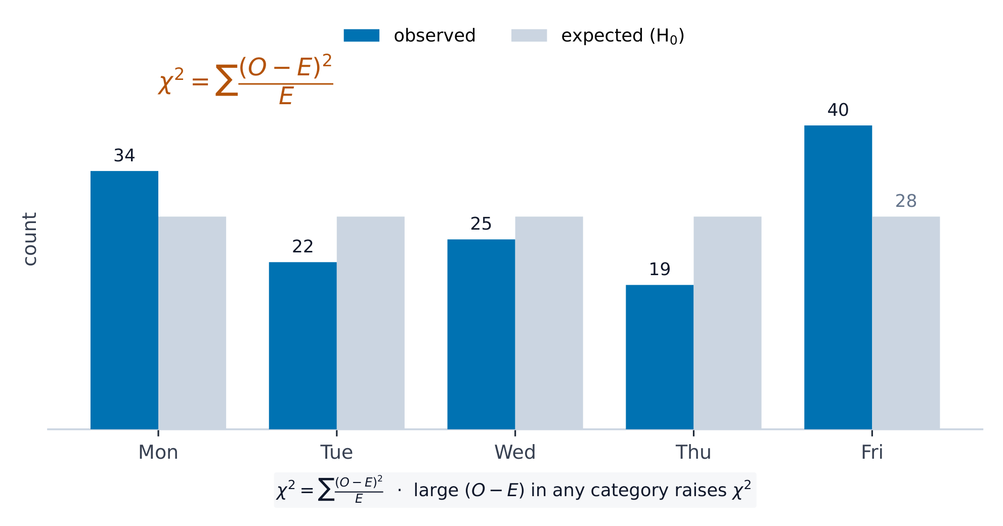
    Source: College Board AP Course and Exam Description · ⁨出典: College Board AP コースおよび試験説明書⁩

    English

    Bar charts 条形图 show the count or proportion of each category as separated bars; a pie chart shows each category's share of the whole. The bar heights (or slices) let you compare categories at a glance. Bars may be ordered by size or by a natural category order.

    日本語

    棒グラフは各カテゴリの個数や割合を独立した棒で示し、円グラフは各カテゴリの全体に対する割合を示す。棒の高さ(または扇形の角度)により、カテゴリを一目で比較できる。棒はサイズ順や自然なカテゴリ順序で並べられることもある。

    Explore · ⁨探索⁩

    Show a categorical variable as a pie chart · ⁨質的変数を円グラフで表示する⁩

    A pie chart turns each category's share of the whole into a slice: a bigger share is a bigger slice, and every slice together makes 100%. It is a picture of a relative-frequency table. · ⁨円グラフは全体のうち各カテゴリーの割合をスライスに変換します。割合が大きいほどスライスの大きさも大きくなり、すべてのスライスを合わせると100%になります。これは相対頻度表の視覚的な表現です。⁩

    1.5

    Representing a Quantitative Variable with Graphs · ⁨グラフによる定量変数の表現⁩

    Syllabus · ⁨シラバス⁩
    English

    Enduring Understanding (UNC-1): Graphical representations and statistics allow us to identify and represent key features of data.

    Learning Objective UNC-1.F: Classify types of quantitative variables. [Skill 2.A]

    • UNC-1.F.1 A discrete variable can take on a countable number of values. The number of values may be finite or countably infinite, as with the counting numbers.
    • UNC-1.F.2 A continuous variable can take on infinitely many values, but those values cannot be counted. No matter how small the interval between two values of a continuous variable, it is always possible to determine another value between them.
      • Illustrative examples for UNC-1.F:
        • A discrete variable:
          • Number of students in a class
        • A continuous variable:
          • Height of a child

    Learning Objective UNC-1.G: Represent quantitative data graphically. [Skill 2.B]

    • UNC-1.G.1 In a histogram, the height of each bar shows the number or proportion of observations that fall within the interval corresponding to that bar. Altering the interval widths can change the appearance of the histogram.
    • UNC-1.G.2 In a stem and leaf plot, each data value is split into a "stem" (the first digit or digits) and a "leaf" (usually the last digit).
    • UNC-1.G.3 A dotplot represents each observation by a dot, with the position on the horizontal axis corresponding to the data value of that observation, with nearly identical values stacked on top of each other.
    • UNC-1.G.4 A cumulative graph represents the number or proportion of a data set less than or equal to a given number.
    • UNC-1.G.5 There are many additional ways to graphically represent distributions of quantitative data.
    日本語

    永続的理解 (UNC-1): グラフや統計は、データの主要な特徴を特定・表現するために用いられる。

    学習目標 UNC-1.F: 定量的変数の種類を分類する。[スキル 2.A]

    • UNC-1.F.1 離散変数は、数えられる数の値をとることができる。その値の数は有限である場合や、自然数のように数え无穷大である場合がある。
    • UNC-1.F.2 連続変数は無限多くの値をとるが、それらの値は数えることができない。連続変数の2つの値間の間隔がいかに小さくても、その間に別の値を特定することは常に可能である。
      • UNC-1.F の例示:
        • 離散変数:
          • クラス内の生徒数
        • 連続変数:
          • 子供の身長

    学習目標 UNC-1.G: グラフを用いて定量的データを表現する。[スキル 2.B]

    • UNC-1.G.1 ヒストグラムにおいて、各棒の高さは、その棒に対応する区間に含まれる観察値の数または割合を示す。区間の幅を変えるとヒストグラムの外見が変わることがある。
    • UNC-1.G.2 ステム&リーフプロットでは、各データ値は「stem」(最初の桁または桁の組み合わせ)と「leaf」(通常は最後の桁)に分割される。
    • UNC-1.G.3 ドットプロットでは、各観察値を点で表し、水平軸上の位置はその観察値のデータ値に対応させ、ほぼ同じ値は積み重ねて表示する。
    • UNC-1.G.4 累積グラフは、与えられた数以下にあるデータセットの数または割合を表す。
    • UNC-1.G.5 定量的データの分布をグラフで表現する方法には、他に多数存在する。

    Source: College Board AP Course and Exam Description · ⁨出典: College Board AP コースおよび試験説明書⁩

    English

    For numbers, use a dotplot 点图, stem-and-leaf plot 茎叶图, or histogram 直方图 (bars over value intervals called bins). These show the distribution 分布 – how the values spread out. A histogram's bin width changes the picture, so choose it to reveal the shape.

    日本語

    数値に対しては、ドットプロット、茎葉図、またはヒストグラム(値区間であるビンの上に置かれた棒)を使用する。これらは分布、つまり値がどのように広がっているかを示す。ヒストグラムのビンの幅は視覚的に変化させるため、形状を明確にするために適切に選択する。

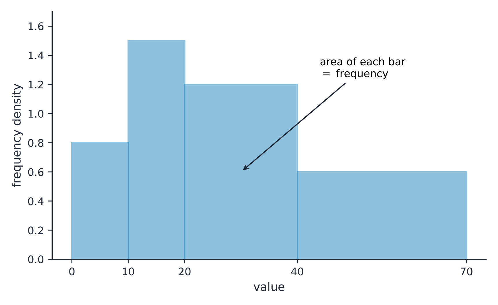
    不均等なクラス幅を持つヒストグラムでは、棒の面積が頻度である
    不均等なクラス幅を持つヒストグラムでは、棒の面積が頻度である
    Explore · ⁨探索⁩

    Explore how bin width shapes a histogram · ⁨ビン幅がヒストグラムの形状に与える影響を調べる⁩

    A histogram groups data into equal-width bins and draws a bar over each. Change the bins and notice how the same data can look jagged (too narrow) or smooth (too wide) — the shape is a choice. · ⁨ヒストグラムはデータを等幅のビンに分類し、各ビンの上に棒を描きます。ビンを変更すると、同じデータでもギザギザ(ビンが狭すぎる場合)や滑らか(ビンが広すぎる場合)に見え方が変わり、形状は選択によるものです。⁩

    Vocabulary · ⁨語彙⁩ Train · ⁨練習する⁩
    English 日本語
    Statistics/stəˈtɪstɪks/ 統計学
    data/ˈdeɪtə/ データ
    variation/ˌveərɪˈeɪʃn/ 変異
    parameter/pəˈræmɪtə/ パラメータ
    statistic/stəˈtɪstɪk/ 統計量
    descriptive statistics/dɪˈskrɪptɪv stəˈtɪstɪks/ 記述統計
    inferential statistics/ɪnfəˈrenʃl stəˈtɪstɪks/ 推定統計学
    variable/ˈveərɪəbl/ 変数
    Categorical/ˌkætɪˈɡɒrɪkl/ 範疇的
    Quantitative/ˈkwɒntɪteɪtɪv/ 定量的
    frequency table/ˈfriːkwənsi ˈteɪbl/ 頻度表
    relative frequency/ˈrelətɪv ˈfriːkwənsi/ 相対周波数
    proportion/prəˈpɔːʃn/ 比例
    Bar charts/bɑː tʃɑːts/ 棒グラフ
    dotplot/ˈdɒtplɒt/ ドットプロット
    stem-and-leaf plot/stem ænd liːf plɒt/ 茎葉図
    histogram/ˈhɪstəɡræm/ ヒストグラム
    1.6

    Describing the Distribution of a Quantitative Variable · ⁨定量変数の分布の記述⁩

    Syllabus · ⁨シラバス⁩
    English

    Enduring Understanding (UNC-1): Graphical representations and statistics allow us to identify and represent key features of data.

    Learning Objective UNC-1.H: Describe the characteristics of quantitative data distributions. [Skill 2.A]

    • UNC-1.H.1 Descriptions of the distribution of quantitative data include shape, center, and variability (spread), as well as any unusual features such as outliers, gaps, clusters, or multiple peaks.
    • UNC-1.H.2 Outliers for one-variable data are data points that are unusually small or large relative to the rest of the data.
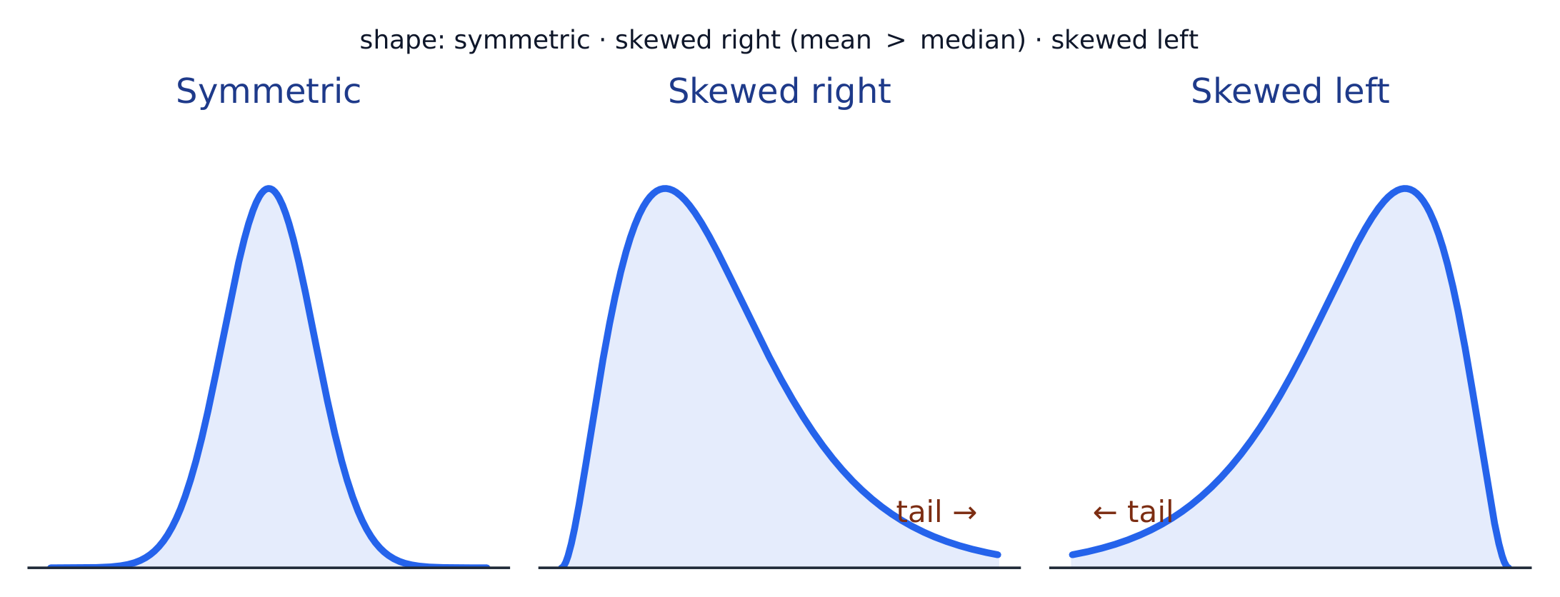
    • UNC-1.H.3 A distribution is skewed to the right (positive skew) if the right tail is longer than the left. A distribution is skewed to the left (negative skew) if the left tail is longer than the right. A distribution is symmetric if the left half is the mirror image of the right half.
    • UNC-1.H.4 Univariate graphs with one main peak are known as unimodal. Graphs with two prominent peaks are bimodal. A graph where each bar height is approximately the same (no prominent peaks) is approximately uniform.
    • UNC-1.H.5 A gap is a region of a distribution between two data values where there are no observed data.
    • UNC-1.H.6 Clusters are concentrations of data usually separated by gaps.
    • UNC-1.H.7 Descriptive statistics does not attribute properties of a data set to a larger population, but may provide the basis for conjectures for subsequent testing.
    日本語

    永続的理解 (UNC-1): グラフや統計は、データの主要な特徴を特定・表現するために用いられる。

    学習目標 UNC-1.H: 定量的データの分布の特徴を説明する。[スキル 2.A]

    • UNC-1.H.1 定量的データの分布の説明には、形状、中心、ばらつき(spread)、および外れ値、ギャップ、クラスター、または複数の山などの異常な特徴が含まれる。
    • UNC-1.H.2 単一変数データの外れ値とは、他のデータに対して異常に小さいまたは大きいデータポイントである。
    • UNC-1.H.3 分布の右側尾が左側尾より長い場合、分布は右に歪んでいる(正の歪み)。左側尾が右側尾より長い場合、分布は左に歪んでいる(負の歪み)。左半分が右半分の鏡像である場合、分布は対称である。
    • UNC-1.H.4 単一の主要な山を持つ単一変数グラフは moda(一峰性)と呼ばれる。2つの目立つ山を持つグラフは bimodal(二峰性)である。各棒の高さがほぼ同じであり(目立つ山がない)、グラフがほぼ均等である場合は uniform(一様分布)である。
    • UNC-1.H.5 ギャップとは、2つのデータ値の間で観測されたデータが存在しない分布の領域である。
    • UNC-1.H.6 クラスターとは、通常ギャップによって分離されているデータの集中部である。
    • UNC-1.H.7 記述統計は、データセットの特性をより大きな母集団に帰属させるものではないが、後続の検定のための推論の基礎を提供することがある。

    Source: College Board AP Course and Exam Description · ⁨出典: College Board AP コースおよび試験説明書⁩

    English

    Describe four things (remember SOCS):

    • Shape 形状: symmetric, or skewed 偏斜 left/right (a long tail on that side), and how many peaks - one main peak is unimodal 单峰, two prominent peaks bimodal 双峰, and roughly equal bars uniform 均匀.
    • Outliers 离群值: unusual values far from the rest.
    • Center: a typical value (mean or median).
    • Spread: how much the values vary (range, IQR, standard deviation).

    Always describe shape/center/spread in context, with units.

    日本語

    4つの要素を記述する(SOCSを思い出す):

    • 形状:対称、または左/右に歪み(その側に長い尾がある)があること、ピークの数がいくつあるか。1つの主要なピークは単峰型、2つの目立つピークは二峰型、ほぼ等しい棒は一様分布である。
    • 外れ値:他の値から大きく離れた異常値。
    • 中心:典型的な値(平均値または中央値)。
    • ばらつき: 値のばらつきの程度(範囲、IQR、標準偏差)。

    常に、単位を添えて、文脈の中で形状・中心・ばらつきを記述すること。

    分布の形状:対称型、右に歪む(右側の長い尾)、または左に歪む
    分布の形状:対称型、右に歪む(右側の長い尾)、または左に歪む
    Vocabulary · ⁨語彙⁩ Train · ⁨練習する⁩
    English 日本語
    distribution/ˌdɪstrɪˈbjuːʃn/ 分配
    Shape/ʃeɪp/ 形状(Shape)
    skewed/skjuːd/ 歪んでいる
    unimodal/ˌʌnɪˈmɒdl/ 単一ピーク分布
    bimodal/baɪˈmɒdl/ 二峰分布
    uniform/ˈjuːnɪfɔːm/ 均一
    Outliers/ˈaʊtlaɪəz/ 外れ値
    mean/miːn/ 平均
    median/ˈmiːdiːən/ 中央値
    interquartile range/ˌɪntəˈkwɔːtaɪl reɪndʒ/ 四分位範囲
    1.7

    Summary Statistics for a Quantitative Variable · ⁨数量変数の要約統計量⁩

    Syllabus · ⁨シラバス⁩
    Enduring UnderstandingLearning ObjectiveEssential Knowledge

    UNC-1
    Graphical representations and statistics allow us to identify and represent key features of data.

    UNC-1.I
    Calculate measures of center and position for quantitative data. [Skill 2.C]

    • UNC-1.I.1 A statistic is a numerical summary of sample data.
    • UNC-1.I.2 The mean is the sum of all the data values divided by the number of values. For a sample, the mean is denoted by $x$-bar: $\bar{x} = \dfrac{1}{n}\sum_{i=1}^{n} x_i$, where $x_i$ represents the $i^{\text{th}}$ data point in the sample and $n$ represents the number of data values in the sample.
    • UNC-1.I.3 The median of a data set is the middle value when data are ordered. When the number of data points is even, the median can take on any value between the two middle values. In AP Statistics, the most commonly used value for the median of a data set with an even number of values is the average of the two middle values.
    • UNC-1.I.4 The first quartile, Q1, is the median of the half of the ordered data set from the minimum to the position of the median. The third quartile, Q3, is the median of the half of the ordered data set from the position of the median to the maximum. Q1 and Q3 form the boundaries for the middle 50% of values in an ordered data set.
    • UNC-1.I.5 The $p^{\text{th}}$ percentile is interpreted as the value that has $p\%$ of the data less than or equal to it.

    UNC-1.J
    Calculate measures of variability for quantitative data. [Skill 2.C]

    • UNC-1.J.1 Three commonly used measures of variability (or spread) in a distribution are the range, interquartile range, and standard deviation.
    • UNC-1.J.2 The range is defined as the difference between the maximum data value and the minimum data value. The interquartile range (IQR) is defined as the difference between the third and first quartiles: $Q3 - Q1$. Both the range and the interquartile range are possible ways of measuring variability of the distribution of a quantitative variable.
    • UNC-1.J.3 Standard deviation is a way to measure variability of the distribution of a quantitative variable. For a sample, the standard deviation is denoted by $s$: $s_x = \sqrt{\dfrac{1}{n-1}\sum(x_i - \bar{x})^2}$. The square of the sample standard deviation, $s^2$, is called the sample variance.
    • UNC-1.J.4 Changing units of measurement affects the values of the calculated statistics.

    UNC-1.K
    Explain the selection of a particular measure of center and/or variability for describing a set of quantitative data. [Skill 4.B]

    • UNC-1.K.1 There are many methods for determining outliers. Two methods frequently used in this course are:
      • UNC-1.K.1.i An outlier is a value greater than $1.5 \times \text{IQR}$ above the third quartile or more than $1.5 \times \text{IQR}$ below the first quartile.
      • UNC-1.K.1.ii An outlier is a value located 2 or more standard deviations above, or below, the mean.
    • UNC-1.K.2 The mean, standard deviation, and range are considered nonresistant (or non-robust) because they are influenced by outliers. The median and IQR are considered resistant (or robust), because outliers do not greatly (if at all) affect their value.

    Source: College Board AP Course and Exam Description · ⁨出典: College Board AP コースおよび試験説明書⁩

    English
    Standard deviation: spread about the mean
    • Center: the mean 均值 $\bar{x}=\dfrac{\sum x_i}{n}$ (average) and the median 中位数 (middle value). The median resists outliers; the mean is pulled toward a skew.
    • Spread: the range, the interquartile range 四分位距 $\text{IQR}=Q_3-Q_1$ (middle 50%), and the standard deviation 标准差 $s_x=\sqrt{\dfrac{\sum(x_i-\bar{x})^2}{n-1}}$ (typical distance from the mean; its square is the variance 方差).
    • The five-number summary 五数概括: min, $Q_1$, median, $Q_3$, max.

    Use resistant measures (median, IQR) for skewed data; mean and standard deviation for roughly symmetric data.

    The percentile 百分位数 of a value is the percent of the data at or below it – so the median is the 50th percentile and $Q_1$ the 25th. A cumulative relative frequency graph 累积相对频率图 makes percentiles easy to read: for each value it plots the proportion of the data at or below it, rising from 0 to 1. Go up from a value to the curve and across to its percentile, or reverse the steps to find the value at a given percentile (the same reading works from a cumulative-frequency table).

    Worked example. For the data $4, 8, 6, 10, 7$: the mean is $\bar{x}=\dfrac{4+8+6+10+7}{5}=\dfrac{35}{5}=7$. Sorting to $4,6,7,8,10$, the median is the middle value, $7$. The mean and median agree here because the data are roughly symmetric.

    日本語
    標準偏差:平均まわりのばらつき
    • 中心: 平均 $\bar{x}=\dfrac{\sum x_i}{n}$(算術平均)と 中央値(真ん中の値)。中央値は外れ値の影響を受けにくく、平均は歪み方向へ引き寄せられる。
    • ばらつき: 範囲、四分位幅 $\text{IQR}=Q_3-Q_1$(中央の50%)、および 標準偏差 $s_x=\sqrt{\dfrac{\sum(x_i-\bar{x})^2}{n-1}}$(平均からの典型的な距離;その二乗が 分散)。
    • 5数要約:最小値、$Q_1$、中央値、$Q_3$、最大値。

    歪んだデータには 抵抗性のある指標(中央値、IQR)を使用し、ほぼ対称的なデータには平均と標準偏差を使用する。

    ある値の 百分位数 は、その値以下にあるデータの割合である。したがって、中央値は第50百分位数であり、$Q_1$は第25百分位数である。累積相対頻度グラフ を用いると百分位数を読み取りやすい。このグラフでは、各値に対してそれ以下のデータの比率をプロットし、0から1まで上昇する曲線を描く。値から垂直に上に進んで曲線に当たり、そこから水平に進んで対応する百分位数を見つけるか、逆に百分位数から値を求めることもできる(累積頻度表でも同様の読み取りが可能)。

    ** worked example.** データ $4, 8, 6, 10, 7$ において、平均は $\bar{x}=\dfrac{4+8+6+10+7}{5}=\dfrac{35}{5}=7$ である。昇順に並べた $4,6,7,8,10$ の中央の値が中央値 $7$ となる。ここではデータがほぼ対称的であるため、平均と中央値は一致している。

    Vocabulary · ⁨語彙⁩ Train · ⁨練習する⁩
    English 日本語
    standard deviation/ˈstændəd ˌdiːvɪˈeɪʃn/ 標準偏差
    variance/ˈveərɪəns/ 分散
    five-number summary/faɪv ˈnʌmbə ˈsʌməri/ 5数要約
    percentile/pəˈsentaɪl/ パーセンタイル
    cumulative relative frequency graph/ˈkjuːmjʊlətɪv ˈrelətɪv ˈfriːkwənsi ɡræf/ 累積相対頻度グラフ
    1.8

    Graphical Representations of Summary Statistics · ⁨要約統計量の視覚的表現⁩

    Syllabus · ⁨シラバス⁩
    Enduring UnderstandingLearning ObjectiveEssential Knowledge

    UNC-1
    Graphical representations and statistics allow us to identify and represent key features of data.

    UNC-1.L
    Represent summary statistics for quantitative data graphically. [Skill 2.B]

    • UNC-1.L.1 Taken together, the minimum data value, the first quartile (Q1), the median, the third quartile (Q3), and the maximum data value make up the five-number summary.
    • UNC-1.L.2 A boxplot is a graphical representation of the five-number summary (minimum, first quartile, median, third quartile, maximum). The box represents the middle 50% of data, with a line at the median and the ends of the box corresponding to the quartiles. Lines ("whiskers") extend from the quartiles to the most extreme point that is not an outlier, and outliers are indicated by their own symbol beyond this.

    UNC-1.M
    Describe summary statistics of quantitative data represented graphically. [Skill 2.A]

    • UNC-1.M.1 Summary statistics of quantitative data, or of sets of quantitative data, can be used to justify claims about the data in context.
    • UNC-1.M.2 If a distribution is relatively symmetric, then the mean and median are relatively close to one another. If a distribution is skewed right, then the mean is usually to the right of the median. If the distribution is skewed left, then the mean is usually to the left of the median.

    Source: College Board AP Course and Exam Description · ⁨出典: College Board AP コースおよび試験説明書⁩

    English

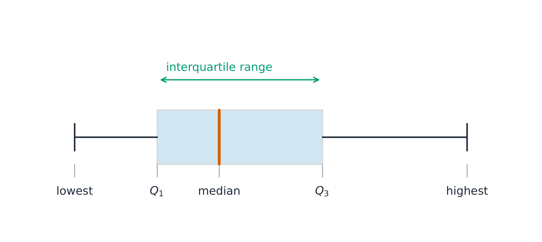
    A boxplot 箱线图 draws the five-number summary: a box from $Q_1$ to $Q_3$ with the median inside, and whiskers to the most extreme non-outlier values. A point is an outlier if it lies more than $1.5\times\text{IQR}$ beyond a quartile – a rule you may be asked to apply. Boxplots are ideal for comparing several groups side by side.

    Worked example. A dataset has $Q_1=20$ and $Q_3=32$, so $\text{IQR}=12$. The outlier fences are $Q_1-1.5(12)=2$ and $Q_3+1.5(12)=50$. Any value below $2$ or above $50$ is flagged as an outlier.

    日本語

    箱ひげ図 は5数要約を描く。$Q_1$ から $Q_3$ までの箱に中央値を含め、最も極端な外れ値ではない値までひげを伸ばす。ある点は四分位数から $1.5\times\text{IQR}$ 以上離れている場合、それは 外れ値 であり、このルールを適用するよう指示されることもある。箱ひげ図は複数のグループを横並びで比較するのに最適である。

    ** worked example.** データセットに $Q_1=20$ と $Q_3=32$ が含まれるため、$\text{IQR}=12$ となる。外れ値の境界値は $Q_1-1.5(12)=2$ と $Q_3+1.5(12)=50$ である。$2$ より小さい値や $50$ より大きい値はすべて外れ値としてフラグ付けされる。

    箱ひげ図は四分位範囲と範囲を示す
    箱ひげ図は四分位範囲と範囲を示す
    箱ひげ図は5数要約を描き、箱はIQRにまたがる
    箱ひげ図は5数要約を描き、箱はIQRにまたがる
    Explore · ⁨探索⁩

    Explore the five-number summary as a boxplot · ⁨5数要約を箱ひげ図として調べる⁩

    Drag $Q_1$, the median, and $Q_3$ to see the box (its length is the IQR) and how the median's position inside the box reveals skew — a median close to $Q_1$ signals a right-skewed distribution. · ⁨$Q_1$、中央値、および$Q_3$をドラッグして、箱(その長さはIQR)を確認します。また、箱内の中央値の位置から歪みを見取ることができます。中央値が$Q_1$に近い場合、右に歪んだ分布を示しています。⁩

    Vocabulary · ⁨語彙⁩ Train · ⁨練習する⁩
    English 日本語
    boxplot/ˈbɒksplɒt/ 箱ひげ図
    normal distribution/ˈnɔːml ˌdɪstrɪˈbjuːʃn/ 正規分布
    1.9

    Comparing Distributions of a Quantitative Variable · ⁨数量変数の分布の比較⁩

    Syllabus · ⁨シラバス⁩
    English

    Enduring Understanding (UNC-1): Graphical representations and statistics allow us to identify and represent key features of data.

    Learning Objective UNC-1.N: Compare graphical representations for multiple sets of quantitative data. [Skill 2.D]

    • UNC-1.N.1 Any of the graphical representations, e.g., histograms, side-by-side boxplots, etc., can be used to compare two or more independent samples on center, variability, clusters, gaps, outliers, and other features.

    Learning Objective UNC-1.O: Compare summary statistics for multiple sets of quantitative data. [Skill 2.D]

    • UNC-1.O.1 Any of the numerical summaries (e.g., mean, standard deviation, relative frequency, etc.) can be used to compare two or more independent samples.
    日本語

    永続的理解 (UNC-1): グラフや統計は、データの主要な特徴を特定・表現するために用いられる。

    学習目標 UNC-1.N: 複数の定量データセットに対して、グラフによる表現を比較する。[スキル 2.D]

    • UNC-1.N.1 ヒストグラム、横並びボックスプロットなど、どのグラフ表現でも、中心、ばらつき、クラスター、ギャップ、外れ値、その他の特徴について、2つ以上の独立したサンプルを比較することができる。
    学習目標 UNC-1.O: 複数の定量データセットの要約統計量を比較する。[スキル 2.D]

    • UNC-1.O.1 平均値、標準偏差、相対頻度などのいずれかの数値要約を用いて、2つ以上の独立したサンプルを比較することができる。
    Source: College Board AP Course and Exam Description · ⁨出典: College Board AP コースおよび試験説明書⁩

    English

    To compare two or more groups, compare shape, center, and spread, and mention outliers – always with comparative words ("Group A has a higher median than Group B") and in context. Do not just describe each group separately; make the comparison explicit.

    日本語

    2つ以上のグループを比較するには、形状、中心、ばらつき を比較し、外れ値にも言及する。常に比較表現(「グループAの中央値はグループBよりも 高い」など)を用いて文脈の中で記述すること。各グループを個別に説明するだけでなく、明確に比較を行うこと。

    Explore · ⁨探索⁩

    Compare distributions with box plots · ⁨箱ひげ図による分布の比較⁩

    A box plot draws the five-number summary. Placing two box plots on the same scale compares their centre (median), spread (IQR = box width) and skew at a glance — the fair way to compare groups. · ⁨箱ひげ図は5数要約を視覚化します。同じスケール上に2つの箱ひげ図を配置することで、中心(中央値)、ばらつき(IQR=箱の幅)、歪みを一目で比較でき、グループ間の公平な比較が可能になります。⁩

    1.10

    The Normal Distribution · ⁨正規分布⁩

    Syllabus · ⁨シラバス⁩
    English

    Enduring Understanding (VAR-2): The normal distribution can be used to represent some population distributions.

    Learning Objective VAR-2.A: Compare a data distribution to the normal distribution model. [Skill 2.D]

    • VAR-2.A.1 A parameter is a numerical summary of a population.
    • VAR-2.A.2 Some sets of data may be described as approximately normally distributed. A normal curve is mound-shaped and symmetric. The parameters of a normal distribution are the population mean, $\mu$, and the population standard deviation, $\sigma$.
    • VAR-2.A.3 For a normal distribution, approximately 68% of the observations are within 1 standard deviation of the mean, approximately 95% of observations are within 2 standard deviations of the mean, and approximately 99.7% of observations are within 3 standard deviations of the mean. This is called the empirical rule.
    • VAR-2.A.4 Many variables can be modeled by a normal distribution.
      • Illustrative examples for VAR-2.A:
        • Variables that can be modeled by a normal distribution:
          • Body temperature
          • Weight of a loaf of bread

    Learning Objective VAR-2.B: Determine proportions and percentiles from a normal distribution. [Skill 3.A]

    • VAR-2.B.1 A standardized score for a particular data value is calculated as (data value − mean)/(standard deviation), and measures the number of standard deviations a data value falls above or below the mean.
    • VAR-2.B.2 One example of a standardized score is a $z$-score, which is calculated as $z\text{-score} = \left(\dfrac{x_i - \mu}{\sigma}\right)$. A $z$-score measures how many standard deviations a data value is from the mean.
    • VAR-2.B.3 Technology, such as a calculator, a standard normal table, or computer-generated output, can be used to find the proportion of data values located on a given interval of a normally distributed random variable.
    • VAR-2.B.4 Given the area of a region under the graph of the normal distribution curve, it is possible to use technology, such as a calculator, a standard normal table, or computer-generated output, to estimate parameters for some populations.

    Learning Objective VAR-2.C: Compare measures of relative position in data sets. [Skill 2.D]

    • VAR-2.C.1 Percentiles and $z$-scores may be used to compare relative positions of points within a data set or between data sets.
    日本語

    長期的理解(VAR-2): 正規分布は、ある集団の分布を表すために使用できる。

    学習目標 VAR-2.A: データの分布を正規分布モデルと比較せよ。[スキル 2.D]

    • VAR-2.A.1 パラメータとは、集団の数的要約のことである。
    • VAR-2.A.2 一部のデータセットは、おおよそ正規分布すると描写されることがある。正規曲線は山型であり対称的である。正規分布のパラメータは、集団平均 $\mu$ および集団標準偏差 $\sigma$ である。
    • VAR-2.A.3 正規分布において、観測値のおよそ68%は平均から標準偏差1個分以内、およそ95%は平均から標準偏差2個分以内、およそ99.7%は平均から標準偏差3個分以内に位置する。これを経験則という。
    • VAR-2.A.4 多くの変数は正規分布によってモデル化できる。
      • *VAR-2.Aの例示:
        • 正規分布でモデル化できる変数:
          • 体温
          • パンの塊の重量

    学習目標 VAR-2.B: 正規分布から割合とパーセンタイルを決定せよ。[スキル 3.A]

    • VAR-2.B.1 特定のデータ値の標準化スコアは、(データ値 − 平均) / (標準偏差) で計算され、そのデータ値が平均から標準偏差いくつ離れているかを示す。
    • VAR-2.B.2 標準化された点数の一例として、$z$-点がある。これは $z\text{-score} = \left(\dfrac{x_i - \mu}{\sigma}\right)$ によって計算される。$z$-点は、データ値が平均からどれだけ標準偏差離れているかを示す。
    • VAR-2.B.3 電卓、標準正規分布表、またはコンピュータ出力のような技術手段を用いて、正規分布する確率変数の与えられた区間に位置するデータ値の割合を求めることができる。
    • VAR-2.B.4 正規分布曲線の下の領域の面積が与えられた場合、電卓、標準正規分布表、またはコンピュータ出力のような技術手段を用いて、いくつかの集団のパラメータを推定することができる。

    学習目標 VAR-2.C: データセット内の相対位置の尺度を比較せよ。[スキル 2.D]

    • VAR-2.C.1 パーセンタイルと$z$-スコアを用いて、データセット内またはデータセット間のポイントの相対位置を比較できる。
    Source: College Board AP Course and Exam Description · ⁨出典: College Board AP コースおよび試験説明書⁩

    English

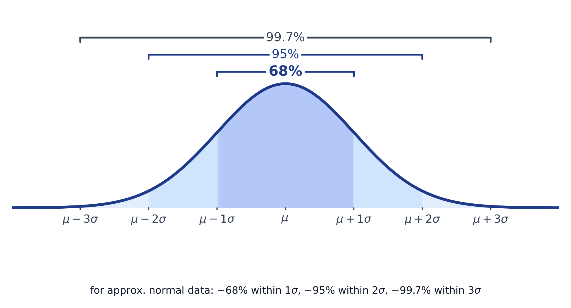
    A normal distribution 正态分布 is a symmetric, bell-shaped model described by its mean $\mu$ and standard deviation $\sigma$. The empirical rule 经验法则 (68–95–99.7): about 68% of values lie within $1\sigma$ of the mean, 95% within $2\sigma$, and 99.7% within $3\sigma$.

    A $z$-score 标准分数 measures how many standard deviations a value is from the mean:

    $$z=\frac{x-\mu}{\sigma}.$$
    Convert to a $z$-score, then use the normal table or technology to find the proportion (area) below, above, or between values – and reverse the process to find a value from a given percentile.

    Worked example. Test scores are normal with $\mu=500$ and $\sigma=100$. A score of $700$ has $z=\dfrac{700-500}{100}=2$. By the empirical rule, $95\%$ of scores lie within $2\sigma$, so $2.5\%$ lie above $700$ – meaning a $700$ is at about the $97.5$th percentile.

    日本語

    正規分布 は対称的で釣鐘型のモデルであり、平均 $\mu$ と標準偏差 $\sigma$ で記述される。経験則(68–95–99.7)によれば、値の約68%が $1\sigma$ 以内に、95%が $2\sigma$ 以内に、99.7%が $3\sigma$ 内にある。

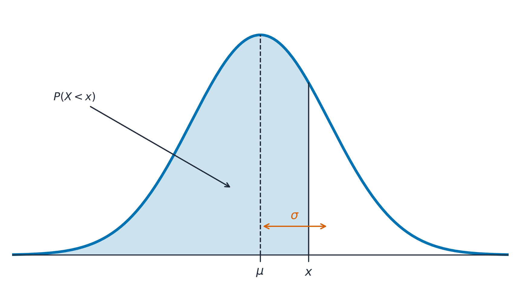
    正規曲線:確率は曲線下の面積であり、平均を中心に配置される
    正規曲線:確率は曲線下の面積であり、平均を中心に配置される

    ある $z$-点 は、ある値が平均から何標準偏差離れているかを測る:

    $$z=\frac{x-\mu}{\sigma}.$$
    $z$-点に変換してから、正規分布表や技術的ツールを使って、値より下、上、または間の 割合(面積)を見つけ、逆の操作を行って特定の百分位数に対応する値を求める。

    ** worked example.** テスト点数は平均 $\mu=500$、標準偏差 $\sigma=100$ の正規分布に従います。得点 $700$ は $z=\dfrac{700-500}{100}=2$ に相当します。経験則により、得分の $95\%$ は $2\sigma$ の範囲内にあり、したがって $2.5\%$ は $700$ より上にあります。つまり、$700$ はおおよそ $97.5$ パーセンタイルに位置しています。

    正規曲線と68-95-99.7の経験則
    正規曲線と68-95-99.7の経験則
    Explore · ⁨探索⁩

    Explore area under the normal curve · ⁨正規曲線下の面積を調べる⁩

    The proportion of data below a value equals the area under the curve to its left. Shade a tail or a central band to see the 68–95–99.7 empirical rule and read a $z$-score as an area. · ⁨ある値以下のデータの割合は、その左側の曲線下の面積に等しいため、尾部分または中央部を着色して68–95–99.7経験則を確認したり、$z$-点数を面積として読み取ったりできます。⁩

    Vocabulary · ⁨語彙⁩ Train · ⁨練習する⁩
    English 日本語
    empirical rule/emˈpɪrɪkl ruːl/ 経験則
    $z$-score/ˈzed skɔː/ $z$-スコア
    1.10

    Exam tips · ⁨試験対策⁩

    English
    • Describe a distribution by shape, center, spread, and outliers (SOCS) — always in context.
    • The mean is pulled by outliers; the median resists them, so prefer the median for skewed data.
    • For a normal distribution use the 68–95–99.7 rule and z-scores $z=\tfrac{x-\mu}{\sigma}$.
    • Compare distributions with side-by-side boxplots and comment on center, spread, and shape.
    • Standard deviation measures a typical distance from the mean; the IQR pairs with the median.
    日本語
    • 分布を 形状、中心、ばらつき、外れ値(SOCS)で記述する — 常に文脈の中で。
    • 平均は外れ値に引き寄せられ、中央値はそれらに抵抗するため、歪んだデータには中央値を好む。
    • 正規分布に対しては、68–95–99.7のルールと z-点 $z=\tfrac{x-\mu}{\sigma}$ を使用する。
    • 横並びの箱ひげ図を用いて分布を比較し、中心、ばらつき、形状についてコメントする。
    • 標準偏差は平均からの典型的な距離を測定し、IQRは中央値と組み合わせて使う。
  • 2

    Exploring Two-Variable Data · ⁨二変量データの探索⁩

    Watch lesson · ⁨レッスンを視聴⁩
    2.1

    Are Two Variables Related?

    Syllabus · ⁨シラバス⁩
    English

    Enduring Understanding (VAR-1): Given that variation may be random or not, conclusions are uncertain.

    Learning Objective VAR-1.D: Identify questions to be answered about possible relationships in data. [Skill 1.A]

    • VAR-1.D.1 Apparent patterns and associations in data may be random or not.
    日本語

    長期的理解(VAR-1): ばらつきがランダムである場合でもそうでない場合でも、結論には不確実性が伴う。

    学習目標 VAR-1.D: データにおける可能性のある関係について答えるべき質問を特定する。[スキル 1.A]

    • VAR-1.D.1 データに見られる明らかなパターンや相関は、偶然のものかもしれないし、そうでないかもしれない。

    Source: College Board AP Course and Exam Description · ⁨出典: College Board AP コースおよび試験説明書⁩

    English

    Two-variable data let us ask whether two characteristics are associated 关联 – whether knowing one tells you something about the other. An explanatory variable 解释变量 (the "input") may help predict a response variable 响应变量 (the "output"). Association is not the same as causation.

    日本語

    Two-variable data let us ask whether two characteristics are associated 关联 – whether knowing one tells you something about the other. An explanatory variable 解释变量 (the "input") may help predict a response variable 响应变量 (the "output"). Association is not the same as causation.

    Vocabulary · ⁨語彙⁩ Train · ⁨練習する⁩
    English 日本語
    associated/əˈsəʊsɪeɪtɪd/ 相関している
    explanatory variable/ekˈsplænətəri ˈveərɪəbl/ 説明変数
    response variable/rɪˈspɒns ˈveərɪəbl/ 応答変数
    2.2

    Two Categorical Variables

    Syllabus · ⁨シラバス⁩
    English

    Enduring Understanding (UNC-1): Graphical representations and statistics allow us to identify and represent key features of data.

    Learning Objective UNC-1.P: Compare numerical and graphical representations for two categorical variables. [Skill 2.D]

    • UNC-1.P.1 Side-by-side bar graphs, segmented bar graphs, and mosaic plots are examples of bar graphs for one categorical variable, broken down by categories of another categorical variable.
    • UNC-1.P.2 Graphical representations of two categorical variables can be used to compare distributions and/or determine if variables are associated.
    • UNC-1.P.3 A two-way table, also called a contingency table, is used to summarize two categorical variables. The entries in the cells can be frequency counts or relative frequencies.
    • UNC-1.P.4 A joint relative frequency is a cell frequency divided by the total for the entire table.
    日本語

    永続的理解 (UNC-1): グラフや統計は、データの主要な特徴を特定・表現するために用いられる。

    学習目標 UNC-1.P: 2つのカテゴリー変数に対する数値的およびグラフによる表現を比較する。[スキル 2.D]

    • UNC-1.P.1 横並び棒グラフ、セグメント棒グラフ、モザイクプロットは、別のカテゴリー変数のカテゴリごとに分解された、1つのカテゴリー変数に対する棒グラフの例である。
    • UNC-1.P.2 2つのカテゴリー変数のグラフによる表現は、分布を比較したり、変数が関連しているかどうかを判定したりするために使用できる。
    • UNC-1.P.3 2変数表(交差表)は、2つのカテゴリ変数を要約するために用いられる。セルの値は頻度または相対頻度であることができる。
    • UNC-1.P.4 連立相対頻度は、あるセルの頻度を全表の総計で割ったものである。

    Source: College Board AP Course and Exam Description · ⁨出典: College Board AP コースおよび試験説明書⁩

    English

    A two-way table 双向表 (contingency table) counts individuals by two categorical variables at once. A marginal distribution 边缘分布 is a row or column total written as a fraction of the grand total (the totals themselves are just counts). Comparing the inside cells shows whether the variables are related.

    日本語

    A two-way table 双向表 (contingency table) counts individuals by two categorical variables at once. A marginal distribution 边缘分布 is a row or column total written as a fraction of the grand total (the totals themselves are just counts). Comparing the inside cells shows whether the variables are related.

    Vocabulary · ⁨語彙⁩ Train · ⁨練習する⁩
    English 日本語
    two-way table/tuː weɪ ˈteɪbl/ 二重表
    marginal distributions/ˈmɑːdʒɪnl ˌdɪstrɪˈbjuːʃnz/ 周辺分布
    2.3

    Comparing Groups with Conditional Distributions

    Syllabus · ⁨シラバス⁩
    English

    Enduring Understanding (UNC-1): Graphical representations and statistics allow us to identify and represent key features of data.

    Learning Objective UNC-1.Q: Calculate statistics for two categorical variables. [Skill 2.C]

    • UNC-1.Q.1 The marginal relative frequencies are the row and column totals in a two-way table divided by the total for the entire table.
    • UNC-1.Q.2 A conditional relative frequency is a relative frequency for a specific part of the contingency table (e.g., cell frequencies in a row divided by the total for that row).

    Learning Objective UNC-1.R: Compare statistics for two categorical variables. [Skill 2.D]

    • UNC-1.R.1 Summary statistics for two categorical variables can be used to compare distributions and/or determine if variables are associated.
    日本語

    永続的理解 (UNC-1): グラフや統計は、データの主要な特徴を特定・表現するために用いられる。

    学習目標 UNC-1.Q: 2つのカテゴリ変数の統計を計算する。[スキル 2.C]

    • UNC-1.Q.1 周辺相対頻度は、2変数表における行と列の合計を全表の総計で割ったものである。
    • UNC-1.Q.2 条件付き相対頻度は、交差表の特定の部分に対する相対頻度である(例:ある行内のセルの頻度をその行の総計で割る)。

    学習目標 UNC-1.R: 2つのカテゴリ変数の統計を比較する。[スキル 2.D]

    • UNC-1.R.1 2つのカテゴリ変数の要約統計は、分布を比較したり、変数間に関連があるかどうかを確認したりするために使用できる。

    Source: College Board AP Course and Exam Description · ⁨出典: College Board AP コースおよび試験説明書⁩

    English

    A conditional distribution 条件分布 is the distribution of one variable within a fixed category of the other (found by dividing each cell by its row or column total). If the conditional distributions differ across groups, the two variables are associated; if they are the same, there is no association. Segmented bar charts 分段条形图 or mosaic plots display them.

    日本語

    A conditional distribution 条件分布 is the distribution of one variable within a fixed category of the other (found by dividing each cell by its row or column total). If the conditional distributions differ across groups, the two variables are associated; if they are the same, there is no association. Segmented bar charts 分段条形图 or mosaic plots display them.

    Vocabulary · ⁨語彙⁩ Train · ⁨練習する⁩
    English 日本語
    conditional distribution/kənˈdɪʃənl ˌdɪstrɪˈbjuːʃn/ 条件付き分布
    Segmented bar charts/seɡˈmentɪd bɑː tʃɑːts/ 区分棒グラフ
    2.4

    Scatterplots for Two Quantitative Variables

    Syllabus · ⁨シラバス⁩
    English

    Enduring Understanding (UNC-1): Graphical representations and statistics allow us to identify and represent key features of data.

    Learning Objective UNC-1.S: Represent bivariate quantitative data using scatterplots. [Skill 2.B]

    • UNC-1.S.1 A bivariate quantitative data set consists of observations of two different quantitative variables made on individuals in a sample or population.
    • UNC-1.S.2 A scatterplot shows two numeric values for each observation, one corresponding to the value on the $x$-axis and one corresponding to the value on the $y$-axis.
    • UNC-1.S.3 An explanatory variable is a variable whose values are used to explain or predict corresponding values for the response variable.

    Enduring Understanding (DAT-1): Regression models may allow us to predict responses to changes in an explanatory variable.

    Learning Objective DAT-1.A: Describe the characteristics of a scatter plot. [Skill 2.A]

    • DAT-1.A.1 A description of a scatter plot includes form, direction, strength, and unusual features.
    • DAT-1.A.2 The direction of the association shown in a scatterplot, if any, can be described as positive or negative.
    • DAT-1.A.3 A positive association means that as values of one variable increase, the values of the other variable tend to increase. A negative association means that as values of one variable increase, values of the other variable tend to decrease.
    • DAT-1.A.4 The form of the association shown in a scatterplot, if any, can be described as linear or non-linear to varying degrees.
    • DAT-1.A.5 The strength of the association is how closely the individual points follow a specific pattern, e.g., linear, and can be shown in a scatterplot. Strength can be described as strong, moderate, or weak.
    • DAT-1.A.6 Unusual features of a scatter plot include clusters of points or points with relatively large discrepancies between the value of the response variable and a predicted value for the response variable.
    日本語

    永続的理解 (UNC-1): グラフや統計は、データの主要な特徴を特定・表現するために用いられる。

    学習目標 UNC-1.S: 散布図を用いて双変量定量データを表現する。[スキル 2.B]

    • UNC-1.S.1 双変量定量データセットは、サンプルや母集団内の個体に対して2つの異なる定量変数を観測したものである。
    • UNC-1.S.2 散布図は、各観測値について2つの数値を示し、それぞれ$x$軸および$y$軸の値に対応している。
    • UNC-1.S.3 説明変数は、応答変数の対応する値を説明または予測するために用いられる変数である。

    持続的理解 (DAT-1): 回帰モデルにより、説明変数の変化に対する応答を予測することが可能となる場合がある。

    学習目標 DAT-1.A: 散布図の特徴を記述する。[スキル 2.A]

    • DAT-1.A.1 散布図の記述には、形、方向、強さ、および異常な特徴が含まれる。
    • DAT-1.A.2 散布図に示される関連の方向(もしあれば)は、正または負として記述できる。
    • DAT-1.A.3 正の関連とは、ある変数の値が増加すると、もう一方の変数の値も増加する傾向にあることを意味する。負の関連とは、ある変数の値が増加すると、もう一方の変数の値が減少する傾向にあることを意味する。
    • DAT-1.A.4 散布図に示される関連の形(もしあれば)は、線形または非線形として、ある程度まで記述できる。
    • DAT-1.A.5 関連の強さは、個々の点が特定のパターン(例:線形)にどれだけ密接に従っているかを示すものであり、散布図で確認できる。強さは「強い」「中程度」「弱い」として記述できる。
    • DAT-1.A.6 散布図の異常な特徴には、点のクラスターや、応答変数の値と予測値との間に大きな乖離がある点が含まれる。

    Source: College Board AP Course and Exam Description · ⁨出典: College Board AP コースおよび試験説明書⁩

    English

    A scatterplot 散点图 plots each individual as a point, explanatory variable on the $x$-axis and response on the $y$-axis. Describe it with DUFS: Direction (positive/negative), Unusual features (outliers, clusters), Form (linear or curved), and Strength (how tightly the points follow the pattern) – always in context.

    日本語

    A scatterplot 散点图 plots each individual as a point, explanatory variable on the $x$-axis and response on the $y$-axis. Describe it with DUFS: Direction (positive/negative), Unusual features (outliers, clusters), Form (linear or curved), and Strength (how tightly the points follow the pattern) – always in context.

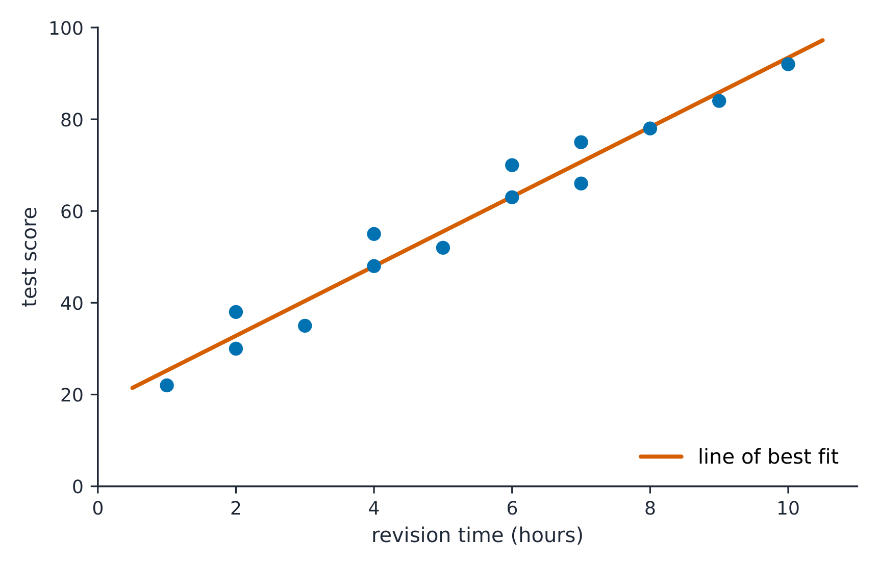
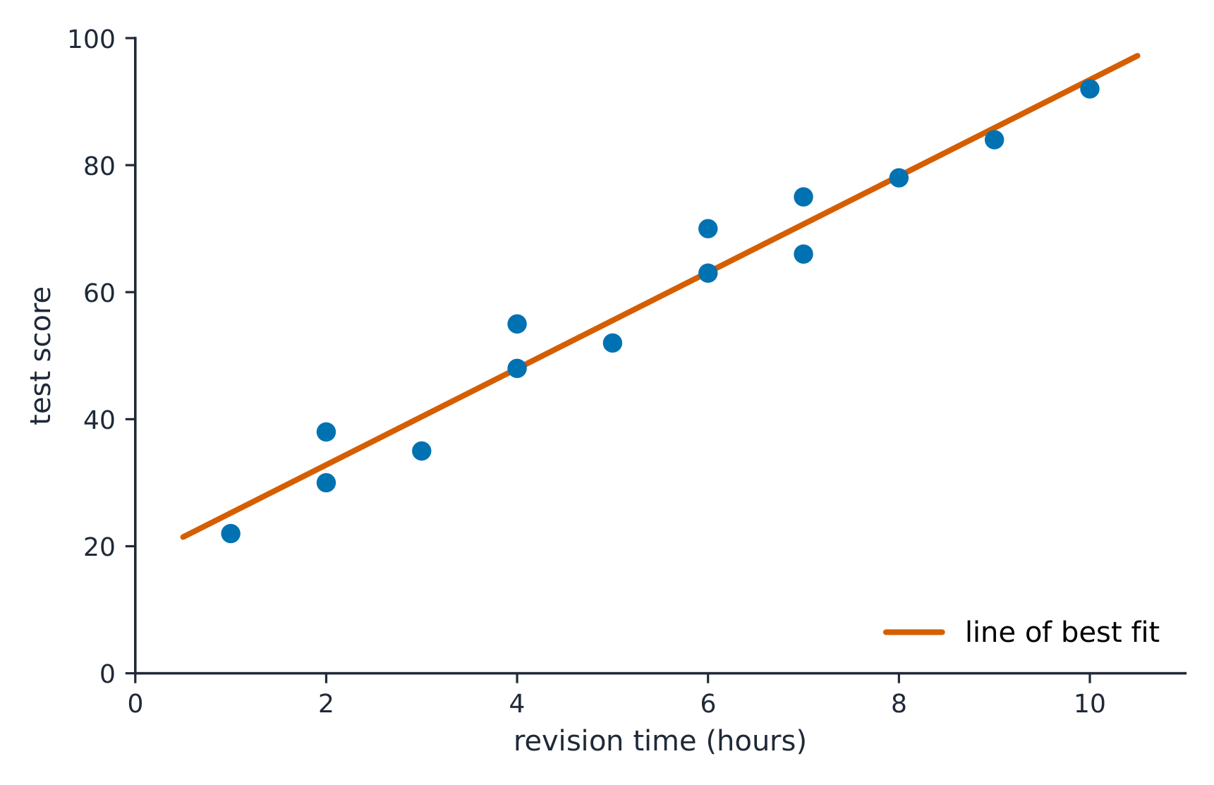
    A line of best fit runs through the middle of the scattered points
    A line of best fit runs through the middle of the scattered points
    Vocabulary · ⁨語彙⁩ Train · ⁨練習する⁩
    English 日本語
    scatterplot/ˈskætəplɒt/ 散布図
    2.5

    Correlation

    Syllabus · ⁨シラバス⁩
    English

    Enduring Understanding (DAT-1): Regression models may allow us to predict responses to changes in an explanatory variable.

    Learning Objective DAT-1.B: Determine the correlation for a linear relationship. [Skill 2.C]

    • DAT-1.B.1 The correlation, $r$, gives the direction and quantifies the strength of the linear association between two quantitative variables.
    • DAT-1.B.2 The correlation coefficient can be calculated by: $r = \dfrac{1}{n-1} \sum \left( \dfrac{x_i - \bar{x}}{s_x} \right) \left( \dfrac{y_i - \bar{y}}{s_y} \right)$. However, the most common way to determine $r$ is by using technology.
    • DAT-1.B.3 A correlation coefficient close to 1 or $-1$ does not necessarily mean that a linear model is appropriate.

    Learning Objective DAT-1.C: Interpret the correlation for a linear relationship. [Skill 4.B]

    • DAT-1.C.1 The correlation, $r$, is unit-free, and always between $-1$ and 1, inclusive. A value of $r = 0$ indicates that there is no linear association. A value of $r = 1$ or $r = -1$ indicates that there is a perfect linear association.
    • DAT-1.C.2 A perceived or real relationship between two variables does not mean that changes in one variable cause changes in the other. That is, correlation does not necessarily imply causation.
    日本語

    持続的理解 (DAT-1): 回帰モデルにより、説明変数の変化に対する応答を予測することが可能となる場合がある。

    学習目標 DAT-1.B: 線形関係の相関を求める。[スキル 2.C]

    • DAT-1.B.1 相関$r$は、2つの定量変数の間の線形関連の方向を示し、その強さを定量化する。
    • DAT-1.B.2 相関係数は $r = \dfrac{1}{n-1} \sum \left( \dfrac{x_i - \bar{x}}{s_x} \right) \left( \dfrac{y_i - \bar{y}}{s_y} \right)$ を用いて計算できる。しかし、$r$ を決定する最も一般的な方法は技術的な手段を用いることである。
    • DAT-1.B.3 相関係数が1または$-1$ に近いからといって、必ずしも線形モデルが適切であることを意味するわけではない。

    学習目標 DAT-1.C: 線形関係の相関を解釈する。[スキル 4.B]

    • DAT-1.C.1 相関$r$是无単位であり、常に$-1$ と1の間(両端を含む)にある。$r = 0$ という値は線形関連がないことを示す。$r = 1$ または$r = -1$ という値は完全な線形関連があることを示す。
    • DAT-1.C.2 2つの変数間に perceived(知覚的・推定的)または real(実在的)な関係があるからといって、ある変数の変化が他方の変数の変化を引き起こすとは限らない。つまり、相関は必ずしも因果関係を意味しない。

    Source: College Board AP Course and Exam Description · ⁨出典: College Board AP コースおよび試験説明書⁩

    English
    What r actually measures

    The correlation coefficient 相关系数 $r$ measures the strength and direction of a linear relationship. It runs from $-1$ to $1$: near $\pm 1$ is strong linear, near $0$ is weak linear. $r$ has no units and does not change if you swap the variables. Warnings: $r$ only measures linear strength, it is not resistant to outliers, and a strong $r$ does not prove causation.

    日本語
    What r actually measures

    The correlation coefficient 相关系数 $r$ measures the strength and direction of a linear relationship. It runs from $-1$ to $1$: near $\pm 1$ is strong linear, near $0$ is weak linear. $r$ has no units and does not change if you swap the variables. Warnings: $r$ only measures linear strength, it is not resistant to outliers, and a strong $r$ does not prove causation.

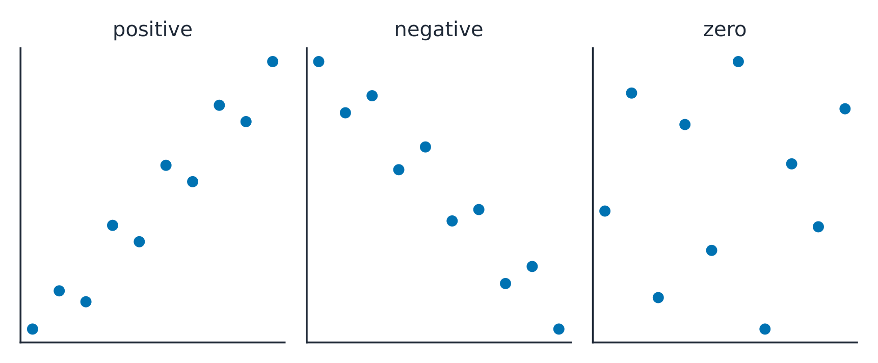
    Positive correlation rises together; negative correlation moves in opposite directions
    Positive correlation rises together; negative correlation moves in opposite directions
    Explore · ⁨探索⁩

    Strength of a linear relationship

    Correlation $r$ runs from $-1$ to $1$: near $\pm1$ the points hug a line, near 0 they scatter. Change it and watch the cloud tighten or spread.

    Vocabulary · ⁨語彙⁩ Train · ⁨練習する⁩
    English 日本語
    correlation coefficient/ˌkɒrɪˈleɪʃn ˌkəʊɪˈfɪʃənt/ 相関係数
    2.6

    Linear Regression Models

    Syllabus · ⁨シラバス⁩
    English

    Enduring Understanding (DAT-1): Regression models may allow us to predict responses to changes in an explanatory variable.

    Learning Objective DAT-1.D: Calculate a predicted response value using a linear regression model. [Skill 2.C]

    • DAT-1.D.1 A simple linear regression model is an equation that uses an explanatory variable, $x$, to predict the response variable, $y$.
    • DAT-1.D.2 The predicted response value, denoted by $\hat{y}$, is calculated as $\hat{y} = a + bx$, where $a$ is the $y$-intercept and $b$ is the slope of the regression line, and $x$ is the value of the explanatory variable.
    • DAT-1.D.3 Extrapolation is predicting a response value using a value for the explanatory variable that is beyond the interval of $x$-values used to determine the regression line. The predicted value is less reliable as an estimate the further we extrapolate.
    日本語

    持続的理解 (DAT-1): 回帰モデルにより、説明変数の変化に対する応答を予測することが可能となる場合がある。

    学習目標 DAT-1.D: 線形回帰モデルを用いて予測応答値を計算する。[スキル 2.C]

    • DAT-1.D.1 単純線形回帰モデルとは、説明変数$x$ を用いて応答変数$y$ を予測するための式である。
    • DAT-1.D.2 予測応答値 $\hat{y}$ は、$\hat{y} = a + bx$ として計算され、ここで $a$ は$y$切片、$b$ は回帰直線の傾き、$x$ は説明変数の値である。
    • DAT-1.D.3 外挿とは、回帰直線を決定するために用いた$x$値の範囲を超えた説明変数の値を用いて応答値を予測することである。外挿の範囲が広くなるほど、予測値は推定値としての信頼性が低下する。

    Source: College Board AP Course and Exam Description · ⁨出典: College Board AP コースおよび試験説明書⁩

    English

    The least-squares regression line 最小二乘回归线 predicts the response: $\hat{y}=a+bx$, where $\hat{y}$ is the predicted response. The slope 斜率 $b$ is the predicted change in $y$ per one-unit increase in $x$; the $y$-intercept 截距 $a$ is the predicted $y$ when $x=0$. Interpret both in context and with units – a graded skill. Avoid extrapolation 外推 (predicting far outside the data).

    Worked example. A study of hours studied ($x$) and test score ($y$) gives $\hat{y}=20+3x$. The slope means each extra hour of study is associated with a predicted $3$-point increase. A student who studies $5$ hours is predicted to score $\hat{y}=20+3(5)=35$.

    日本語

    The least-squares regression line 最小二乘回归线 predicts the response: $\hat{y}=a+bx$, where $\hat{y}$ is the predicted response. The slope 斜率 $b$ is the predicted change in $y$ per one-unit increase in $x$; the $y$-intercept 截距 $a$ is the predicted $y$ when $x=0$. Interpret both in context and with units – a graded skill. Avoid extrapolation 外推 (predicting far outside the data).

    Worked example. A study of hours studied ($x$) and test score ($y$) gives $\hat{y}=20+3x$. The slope means each extra hour of study is associated with a predicted $3$-point increase. A student who studies $5$ hours is predicted to score $\hat{y}=20+3(5)=35$.

    Explore · ⁨探索⁩

    Fit a least-squares line

    A regression line is the best straight-line fit, minimising the squared vertical distances. Its slope predicts how $y$ changes per unit of $x$.

    Vocabulary · ⁨語彙⁩ Train · ⁨練習する⁩
    English 日本語
    least-squares regression line/liːst skweəz rɪˈɡreʃn laɪn/ 最小二乗回帰直線
    slope/sləʊp/ 傾き
    y-intercept/waɪ ˌɪntəˈsept/ y切片
    extrapolation/ekˈstræpəleɪʃn/ 外挿
    2.7

    Residuals

    Syllabus · ⁨シラバス⁩
    English

    Enduring Understanding (DAT-1): Regression models may allow us to predict responses to changes in an explanatory variable.

    Learning Objective DAT-1.E: Represent differences between measured and predicted responses using residual plots. [Skill 2.B]

    • DAT-1.E.1 The residual is the difference between the actual value and the predicted value: $\text{residual} = y - \hat{y}$.
    • DAT-1.E.2 A residual plot is a plot of residuals versus explanatory variable values or predicted response values.

    Learning Objective DAT-1.F: Describe the form of association of bivariate data using residual plots. [Skill 2.A]

    • DAT-1.F.1 Apparent randomness in a residual plot for a linear model is evidence of a linear form to the association between the variables.
    • DAT-1.F.2 Residual plots can be used to investigate the appropriateness of a selected model.
    日本語

    持続的理解 (DAT-1): 回帰モデルにより、説明変数の変化に対する応答を予測することが可能となる場合がある。

    学習目標 DAT-1.E: 残差プロットを用いて、測定値と予測値の間の違いを表現する。[スキル 2.B]

    • DAT-1.E.1 残差は、実際の値と予測値の差である:$\text{residual} = y - \hat{y}$。
    • DAT-1.E.2 残差プロットとは、残差を説明変数の値または予測応答値に対してプロットしたものである。

    学習目標 DAT-1.F: 残差プロットを用いて双変量データの相関の形を説明する。[スキル 2.A]

    • DAT-1.F.1 線形モデルの残差プロットに見られる明らかなランダム性は、変数間の関連が線形であることを裏付ける証拠となる。
    • DAT-1.F.2 残差プロットを用いて、選択されたモデルが適切かどうかを検証することができる。

    Source: College Board AP Course and Exam Description · ⁨出典: College Board AP コースおよび試験説明書⁩

    English
    Least-squares regression

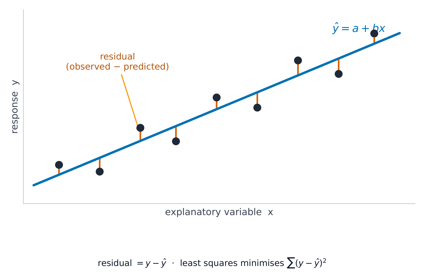
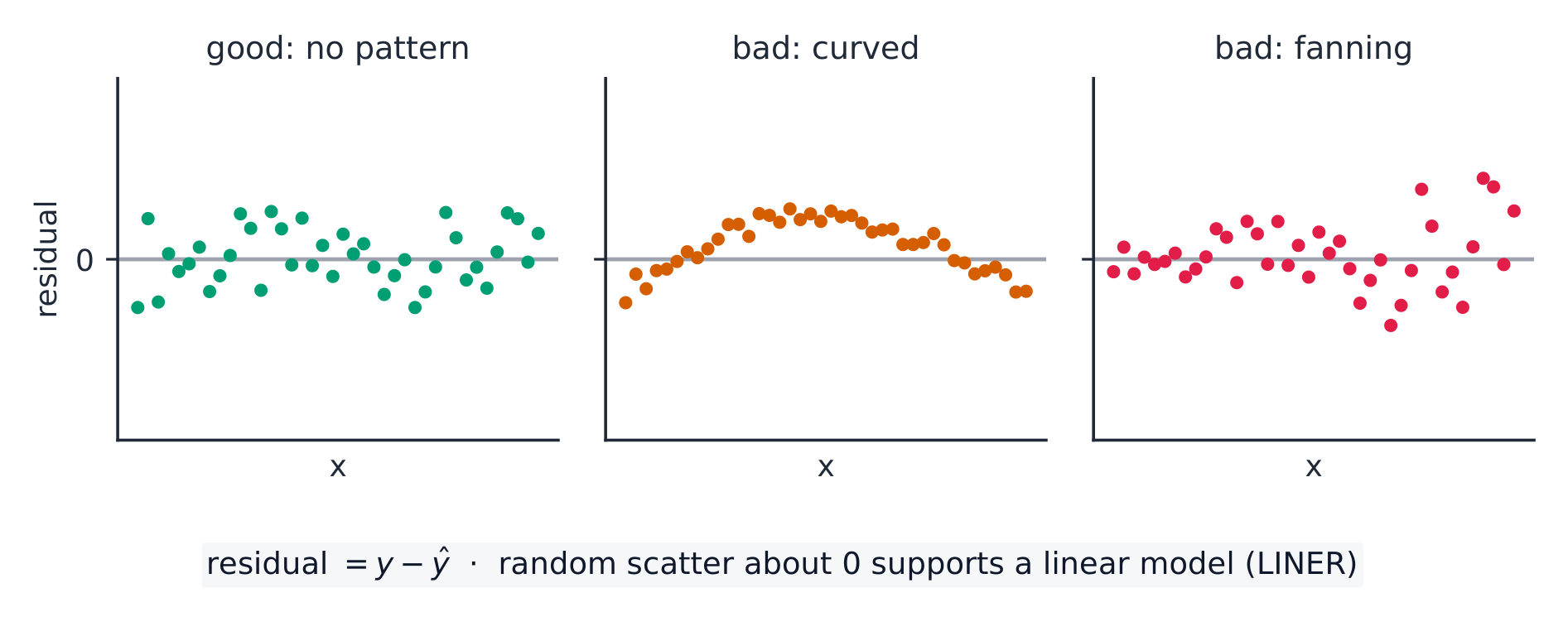
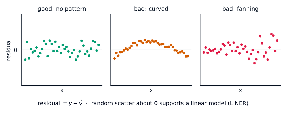
    A residual 残差 is actual minus predicted, $y-\hat{y}$: how far a point sits above (+) or below (−) the line. A residual plot 残差图 graphs residuals against $x$. If it shows no pattern (random scatter), a linear model is appropriate; a curved or fanning pattern means the linear model is a poor fit.

    Worked example. Continuing the study above, a student who studied $5$ hours actually scored $40$. The residual is $y-\hat{y}=40-35=+5$: the line under-predicted by $5$ points, so this point sits above the line.

    日本語
    Least-squares regression

    A residual 残差 is actual minus predicted, $y-\hat{y}$: how far a point sits above (+) or below (−) the line. A residual plot 残差图 graphs residuals against $x$. If it shows no pattern (random scatter), a linear model is appropriate; a curved or fanning pattern means the linear model is a poor fit.

    Worked example. Continuing the study above, a student who studied $5$ hours actually scored $40$. The residual is $y-\hat{y}=40-35=+5$: the line under-predicted by $5$ points, so this point sits above the line.

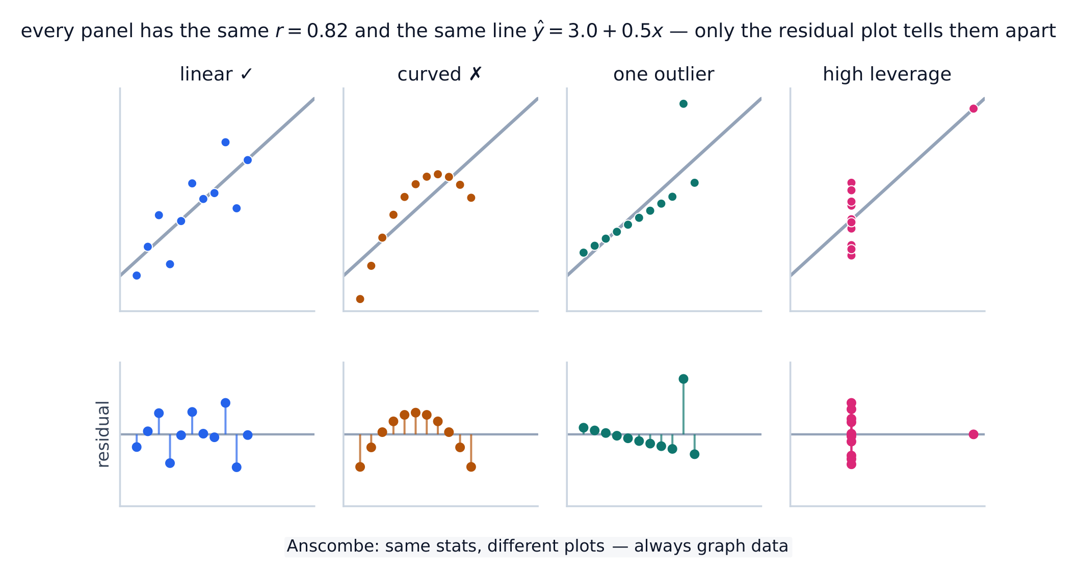
    Four datasets with identical r and regression line but four different shapes
    A caution about $r$ and the line: all four datasets have the same $r=0.82$ and the same $\hat{y}=3.0+0.5x$, yet only the first is genuinely linear. The scatterplots barely differ — the residual plot below each is what exposes the curve, the outlier, and the high-leverage point.
    Vocabulary · ⁨語彙⁩ Train · ⁨練習する⁩
    English 日本語
    residual/rɪˈsɪdʒuːəl/ 残差
    residual plot/rɪˈsɪdʒuːəl plɒt/ 残差プロット
    2.8

    Least-Squares Regression and Its Fit

    Syllabus · ⁨シラバス⁩
    Enduring UnderstandingLearning ObjectiveEssential Knowledge

    DAT-1
    Regression models may allow us to predict responses to changes in an explanatory variable.

    DAT-1.G
    Estimate parameters for the least-squares regression line model. [Skill 2.C]

    • DAT-1.G.1 The least-squares regression model minimizes the sum of the squares of the residuals and contains the point $(\bar{x}, \bar{y})$.
    • DAT-1.G.2 The slope, $b$, of the regression line can be calculated as $b = r \left( \dfrac{s_y}{s_x} \right)$ where $r$ is the correlation between $x$ and $y$, $s_y$ is the sample standard deviation of the response variable, $y$, and $s_x$ is the sample standard deviation of the explanatory variable, $x$.
    • DAT-1.G.3 Sometimes, the $y$-intercept of the line does not have a logical interpretation in context.
    • DAT-1.G.4 In simple linear regression, $r^2$ is the square of the correlation, $r$. It is also called the coefficient of determination. $r^2$ is the proportion of variation in the response variable that is explained by the explanatory variable in the model.

    DAT-1.H
    Interpret coefficients for the least-squares regression line model. [Skill 4.B]

    • DAT-1.H.1 The coefficients of the least-squares regression model are the estimated slope and $y$-intercept.
    • DAT-1.H.2 The slope is the amount that the predicted $y$-value changes for every unit increase in $x$.
    • DAT-1.H.3 The $y$-intercept value is the predicted value of the response variable when the explanatory variable is equal to $0$. The formula for the $y$-intercept, $a$, is $a = \bar{y} - b\bar{x}$.

    Source: College Board AP Course and Exam Description · ⁨出典: College Board AP コースおよび試験説明書⁩

    English

    The line minimizes the sum of squared residuals. Its fit is measured by:

    • $s$, the standard deviation of the residuals – the typical prediction error, in the response's units.
    • $r^2$, the coefficient of determination 决定系数 – the proportion of the variation in $y$ that the linear model explains (a value between $0$ and $1$; multiply by $100$ to state it as a percent). Report it in context: "$r^2 = 0.81$ means 81% of the variation in $y$ is explained by the linear relationship with $x$."
    日本語
    The least-squares line minimizes the sum of squared residuals
    The least-squares line minimizes the sum of squared residuals

    The line minimizes the sum of squared residuals. Its fit is measured by:

    • $s$, the standard deviation of the residuals – the typical prediction error, in the response's units.
    • $r^2$, the coefficient of determination 决定系数 – the proportion of the variation in $y$ that the linear model explains (a value between $0$ and $1$; multiply by $100$ to state it as a percent). Report it in context: "$r^2 = 0.81$ means 81% of the variation in $y$ is explained by the linear relationship with $x$."
    Vocabulary · ⁨語彙⁩ Train · ⁨練習する⁩
    English 日本語
    coefficient of determination/ˌkəʊɪˈfɪʃənt ɒv dɪˌtɜːmɪˈneɪʃn/ 決定係数
    2.9

    Departures from Linearity

    Syllabus · ⁨シラバス⁩
    English

    Enduring Understanding (DAT-1): Regression models may allow us to predict responses to changes in an explanatory variable.

    Learning Objective DAT-1.I: Identify influential points in regression. [Skill 2.A]

    • DAT-1.I.1 An outlier in regression is a point that does not follow the general trend shown in the rest of the data and has a large residual when the Least Squares Regression Line (LSRL) is calculated.
    • DAT-1.I.2 A high-leverage point in regression has a substantially larger or smaller $x$-value than the other observations have.
    • DAT-1.I.3 An influential point in regression is any point that, if removed, changes the relationship substantially. Examples include much different slope, $y$-intercept, and/or correlation. Outliers and high leverage points are often influential.

    Learning Objective DAT-1.J: Calculate a predicted response using a least-squares regression line for a transformed data set. [Skill 2.C]

    • DAT-1.J.1 Transformations of variables, such as evaluating the natural logarithm of each value of the response variable or squaring each value of the explanatory variable, can be used to create transformed data sets, which may be more linear in form than the untransformed data.
    • DAT-1.J.2 Increased randomness in residual plots after transformation of data and/or movement of $r^2$ to a value closer to 1 offers evidence that the least-squares regression line for the transformed data is a more appropriate model to use to predict responses to the explanatory variable than the regression line for the untransformed data.
    日本語

    持続的理解 (DAT-1): 回帰モデルにより、説明変数の変化に対する応答を予測することが可能となる場合がある。

    学習目標 DAT-1.I: 回帰における影響のある点を同定する。[スキル 2.A]

    • DAT-1.I.1 回帰における外れ値とは、データ全体の一般的な傾向に従わず、最小二乗回帰直線(LSRL)を計算した際に大きな残差を持つ点である。
    • DAT-1.I.2 回帰における高レバージポイントは、他の観測値よりも著しく大きいか小さい $x$ 値を持つ。
    • DAT-1.I.3 回帰における影響のある点は、除外すると関係性が大きく変わる点である。例として、著しく異なる傾き、$y$切片、および/または相関が挙げられる。外れ値や高レバレッジポイントはしばしば影響がある。

    学習目標 DAT-1.J: 変換されたデータセットに対して、最小二乗回帰直線を用いて予測応答を計算する。[スキル 2.C]

    • DAT-1.J.1 変数の変換(例:応答変数の各値の自然対数を評価する、または説明変数の各値を二乗する)により、変換されたデータセットを作成できる。これらは未変換のデータよりも線形に近い形になる可能性がある。
    • DAT-1.J.2 データ変換後、残差プロットにおける不規則性の増加や、$r^2$ の値が1に近づくことの変化は、変換されたデータの最小二乗回帰直線が、未変換データの回帰直線よりも説明変数に対する応答を予測するより適切なモデルであることを示す証拠となる。

    Source: College Board AP Course and Exam Description · ⁨出典: College Board AP コースおよび試験説明書⁩

    English

    Some points strongly affect the line. A high-leverage 高杠杆 point has an extreme $x$-value; an influential 有影响的 point noticeably changes the slope or $r$ when removed; an outlier here is a point with a large residual. When the pattern is curved, transform a variable (e.g. take a log) to straighten it, then fit a line to the transformed data.

    日本語

    Some points strongly affect the line. A high-leverage 高杠杆 point has an extreme $x$-value; an influential 有影响的 point noticeably changes the slope or $r$ when removed; an outlier here is a point with a large residual. When the pattern is curved, transform a variable (e.g. take a log) to straighten it, then fit a line to the transformed data.

    Vocabulary · ⁨語彙⁩ Train · ⁨練習する⁩
    English 日本語
    high-leverage/haɪ ˈliːvərɪdʒ/ 高レバレッジ
    influential/ˌɪnfluːˈenʃl/ 影響のある
    2.9

    Exam tips

    • On a scatterplot describe direction, form, strength, and outliers; $r$ ranges $-1$ to $1$.
    • Correlation is not causation — a lurking variable can drive both.
    • Interpret the slope of the least-squares line in context ("per one unit of $x$, predicted $y$ changes by $b$").
    • Check a residual plot: no pattern means a line fits; a curve means it does not. Avoid extrapolation.
    • $r^2$ is the fraction of variation in $y$ explained by the model.
  • 3

    Collecting Data · ⁨データ収集⁩

    Watch lesson · ⁨レッスンを視聴⁩
    3.1

    Can We Trust the Data We Collected? · ⁨収集したデータを信頼できるか?⁩

    Syllabus · ⁨シラバス⁩
    English

    Enduring Understanding (VAR-1): Given that variation may be random or not, conclusions are uncertain.

    Learning Objective VAR-1.E: Identify questions to be answered about data collection methods. [Skill 1.A]

    • VAR-1.E.1 Methods for data collection that do not rely on chance result in untrustworthy conclusions.
    日本語

    長期的理解(VAR-1): ばらつきがランダムである場合でもそうでない場合でも、結論には不確実性が伴う。

    学習目標 VAR-1.E: データ収集方法に関する解答すべき質問を同定する。[スキル 1.A]

    • VAR-1.E.1 偶然性に依存しないデータ収集方法では、信頼できない結論が導かれる。

    Source: College Board AP Course and Exam Description · ⁨出典: College Board AP コースおよび試験説明書⁩

    English

    A conclusion is only as good as the data behind it. How data are collected decides what you may conclude – whether you can generalize to a population 总体, and whether you can claim cause and effect. Poorly collected data can be worse than none.

    日本語

    結論は、それを裏付けるデータの品質と同じくらいです。データ収集方法が何 conclusiónを導き出せるかを決定します——母集団への一般化が可能かどうか、そして因果関係を主張できるかどうかです。不善なデータ収集は、データなしであることよりも悪い結果をもたらすことがあります。

    3.2

    Observational Studies and Experiments · ⁨観察研究と実験⁩

    Syllabus · ⁨シラバス⁩
    English

    Enduring Understanding (DAT-2): The way we collect data influences what we can and cannot say about a population.

    Learning Objective DAT-2.A: Identify the type of a study. [Skill 1.C]

    • DAT-2.A.1 A population consists of all items or subjects of interest.
    • DAT-2.A.2 A sample selected for study is a subset of the population.
    • DAT-2.A.3 In an observational study, treatments are not imposed. Investigators examine data for a sample of individuals (retrospective) or follow a sample of individuals into the future collecting data (prospective) in order to investigate a topic of interest about the population. A sample survey is a type of observational study that collects data from a sample in an attempt to learn about the population from which the sample was taken.
    • DAT-2.A.4 In an experiment, different conditions (treatments) are assigned to experimental units (participants or subjects).

    Learning Objective DAT-2.B: Identify appropriate generalizations and determinations based on observational studies. [Skill 4.A]

    • DAT-2.B.1 It is only appropriate to make generalizations about a population based on samples that are randomly selected or otherwise representative of that population.
    • DAT-2.B.2 A sample is only generalizable to the population from which the sample was selected.
    • DAT-2.B.3 It is not possible to determine causal relationships between variables using data collected in an observational study.
    日本語

    持続的理解 (DAT-2): データの収集方法は、集団について何が言え、何が言えないかに影響を与える。

    学習目標 DAT-2.A: 研究のタイプを同定する。[スキル 1.C]

    • DAT-2.A.1 集団は、関心のあるすべての項目や対象者で構成される。
    • DAT-2.A.2 研究のために選択されたサンプルは、集団の部分集合である。
    • DAT-2.A.3 観察研究では、処置が加えられない。研究者は、集団に関する関心事を調査するために、個人サンプルのデータを retrospectively に検討するか、prospective に個人サンプルを追跡してデータを収集する。サンプル調査とは、サンプルから得られた集団について学ぶことを目的として、サンプルからデータを収集する観察研究の一種である。
    • DAT-2.A.4 実験では、異なる条件(処置)が実験単体(参加者や被験者)に割り当てられる。

    学習目標 DAT-2.B: 観察研究に基づいた適切な一般化と判定を同定する。[スキル 4.A]

    • DAT-2.B.1 集団に対する一般化を行うのは、無作為に選択されたサンプル、またはその集団を代表する他のサンプルの場合のみ適切である。
    • DAT-2.B.2 サンプルは、サンプルが選択された集団にのみ一般化可能である。
    • DAT-2.B.3 観察研究で収集されたデータを用いて、変数間の因果関係を判定することは不可能である。

    Source: College Board AP Course and Exam Description · ⁨出典: College Board AP コースおよび試験説明書⁩

    English
    • In an observational study 观察性研究 you measure individuals without trying to influence them. It can show association, but not causation, because lurking variables may explain the link.
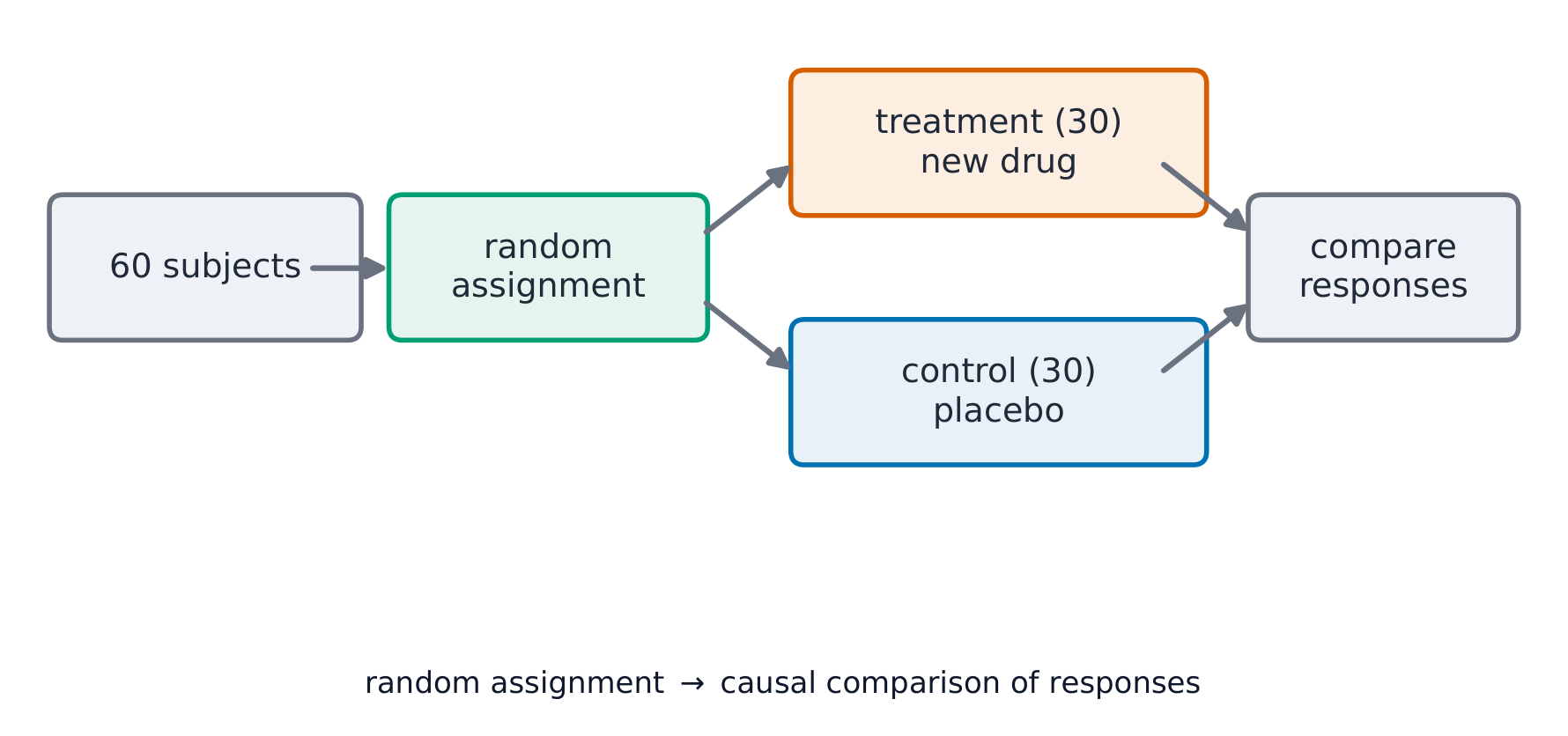
    • In an experiment 实验 you deliberately impose a treatment 处理 and compare responses. A well-designed experiment can establish cause and effect.
    日本語
    • 観察研究では、対象に影響を与えずに測定します。関連性を示すことはできますが、隠れた変数が関係を説明する可能性があるため、因果関係までは示せません。
    • 実験では、意図的に処置を加え、応答を比較します。設計の優れた実験は因果関係を確立できる可能性があります。
    Explore · ⁨探索⁩

    Observational study or experiment? · ⁨観察研究と実験の違い⁩

    In an experiment the researcher imposes a treatment (and can show cause); an observational study only records what already happens (and can show association, not cause). · ⁨実験では研究者が処置を与え(因果関係を示せる)、観察研究では既に起こっている事象を記録するのみであり(関連性は示せるが因果関係は示せない)です。⁩

    3.3

    Random Sampling · ⁨無作為抽出⁩

    Syllabus · ⁨シラバス⁩
    English

    Enduring Understanding (DAT-2): The way we collect data influences what we can and cannot say about a population.

    Learning Objective DAT-2.C: Identify a sampling method, given a description of a study. [Skill 1.C]

    • DAT-2.C.1 When an item from a population can be selected only once, this is called sampling without replacement. When an item from the population can be selected more than once, this is called sampling with replacement.
    • DAT-2.C.2 A simple random sample (SRS) is a sample in which every group of a given size has an equal chance of being chosen. This method is the basis for many types of sampling mechanisms. A few examples of mechanisms used to obtain SRSs include numbering individuals and using a random number generator to select which ones to include in the sample, ignoring repeats, using a table of random numbers, or drawing a card from a deck without replacement.
    • DAT-2.C.3 A stratified random sample involves the division of a population into separate groups, called strata, based on shared attributes or characteristics (homogeneous grouping). Within each stratum a simple random sample is selected, and the selected units are combined to form the sample.
    • DAT-2.C.4 A cluster sample involves the division of a population into smaller groups, called clusters. Ideally, there is heterogeneity within each cluster, and clusters are similar to one another in their composition. A simple random sample of clusters is selected from the population to form the sample of clusters. Data are collected from all observations in the selected clusters.
    • DAT-2.C.5 A systematic random sample is a method in which sample members from a population are selected according to a random starting point and a fixed, periodic interval.
    • DAT-2.C.6 A census selects all items/subjects in a population.

    Learning Objective DAT-2.D: Explain why a particular sampling method is or is not appropriate for a given situation. [Skill 1.C]

    • DAT-2.D.1 There are advantages and disadvantages for each sampling method depending upon the question that is to be answered and the population from which the sample will be drawn.
    日本語

    持続的理解 (DAT-2): データの収集方法は、集団について何が言え、何が言えないかに影響を与える。

    学習目標 DAT-2.C: 研究の説明に基づいてサンプリング方法を同定する。[スキル 1.C]

    • DAT-2.C.1 母集団からの要素が一度しか選択できない場合、これを復元なし抽出という。母集団からの要素が複数回選択できる場合、これを復元あり抽出という。
    • DAT-2.C.2 単純無作為サンプル(SRS)とは、特定のサイズを持つグループすべてが選ばれる確率が等しいサンプルである。この手法は多くのサンプリングメカニズムの基礎となっている。SRSを取得するためのメカニズムの例には、個人に番号を振って無作為数生成器を使用してサンプルに含めるものを選び、重複を無視する、無作為数表を使用する、あるいは無放回でデッキからカードを引き出すなどが挙げられる。
    • DAT-2.C.3 層化無作為抽出は、共通する属性や特徴(均質なグループ分け)に基づいて母集団を別々のグループである「層」に分割する方法です。各層内では単純無作為抽出が行われ、選ばれた単位が組み合わさってサンプルとなります。
    • DAT-2.C.4 クラスター抽出は、母集団をより小さなグループである「クラスター」に分割する方法です。理想的には、各クラスター内に多様性があり、クラスター同士の構成が類似している必要があります。母集団からクラスターの単純無作為サンプルが選抜され、これがクラスターのサンプルとなります。選ばれたクラスター内のすべての観察値からデータ収集が行われます。
    • DAT-2.C.5 系統抽出とは、母集団からのサンプル成员を、ランダムな開始点と一定の周期間隔に従って選抜する方法です。
    • DAT-2.C.6 全数調査は、母集団内のすべての項目・対象者を選抜します。

    学習目標 DAT-2.D: 特定の状況に対してどのサンプリング方法が適切か、または不適切かを説明する。[スキル 1.C]

    • DAT-2.D.1 各サンプリング方法には長所と短所があり、それらは解答すべき質問やサンプルの出所となる母集団によって異なります。

    Source: College Board AP Course and Exam Description · ⁨出典: College Board AP コースおよび試験説明書⁩

    English

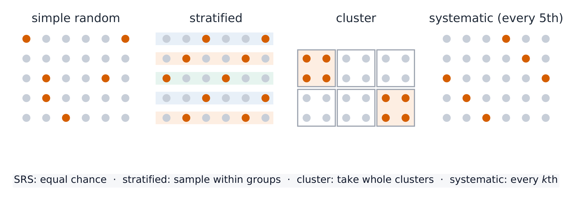
    To learn about a population you take a sample 样本. Random sampling 随机抽样 protects against selection bias 偏差 and lets you generalize (it cannot fix undercoverage, nonresponse, or response bias — see below). Common designs:

    • Simple random sample (SRS) 简单随机样本: every group of the chosen size is equally likely.
    • Stratified 分层: split the population into similar strata, then sample within each.
    • Cluster 整群: split into clusters, randomly choose whole clusters.
    • Systematic 系统: pick every $k$th individual from a random start.

    A convenience sample 方便样本 or voluntary response sample is not random and is biased.

    Worked example. To survey a school, an administrator lists all students by grade and randomly selects $20$ from each grade. This is a stratified sample – the grades are the strata – which guarantees every grade is represented, unlike an SRS that might by chance draw few from one grade.

    日本語

    母集団について学ぶためにはサンプルを採取します。無作為抽出は選択バイアスを防ぎ、一般化を可能にしますが(過小カバー、非回答、回答バイアスは修正できません——後述)、一般的なデザインとして以下のものが用いられます:

    • 単純無作為サンプリング (SRS):指定されたサイズのすべてのグループが等しい確率で選ばれます。
    • 層別: 母集団を類似した層に分け、各層内でサンプリングします。
    • クラスター: クラスターに分け、無作為に全体クラスターを選びます。
    • 系統: 無作為な開始点后に、$k$番目の個人を順に選びます。
    4つの無作為抽出デザイン:誰が選ばれ、どのように選ばれるか
    4つの無作為抽出デザイン:誰が選ばれ、どのように選ばれるか

    利便標本または自発的応答標本は無作為ではなく、バイアスを含みます。

    ** worked example.** 学校を調査するために、管理者は学年ごとに全生徒をリストアップし、各学年から $20$ を無作為に抽出します。これは 層化標本 です——学年は層であり、SRS(単純無作為抽出)のように偶然ある学年からの抽出数が少なくなることを防ぎます。

    無作為な結果:公平な条件下ではサイコロの各面が出る確率が等しい
    無作為な結果:公平な条件下ではサイコロの各面が出る確率が等しい
    3.4

    When Sampling Goes Wrong · ⁨抽出が失敗するケース⁩

    Syllabus · ⁨シラバス⁩
    English

    Enduring Understanding (DAT-2): The way we collect data influences what we can and cannot say about a population.

    Learning Objective DAT-2.E: Identify potential sources of bias in sampling methods. [Skill 1.C]

    • DAT-2.E.1 Bias occurs when certain responses are systematically favored over others.
    • DAT-2.E.2 When a sample is comprised entirely of volunteers or people who choose to participate, the sample will typically not be representative of the population (voluntary response bias).
    • DAT-2.E.3 When part of the population has a reduced chance of being included in the sample, the sample will typically not be representative of the population (undercoverage bias).
    • DAT-2.E.4 Individuals chosen for the sample for whom data cannot be obtained (or who refuse to respond) may differ from those for whom data can be obtained (nonresponse bias).
    • DAT-2.E.5 Problems in the data gathering instrument or process result in response bias. Examples include questions that are confusing or leading (question wording bias) and self-reported responses.
    • DAT-2.E.6 Non-random sampling methods (for example, samples chosen by convenience or voluntary response) introduce potential for bias because they do not use chance to select the individuals.
    日本語

    持続的理解 (DAT-2): データの収集方法は、集団について何が言え、何が言えないかに影響を与える。

    学習目標 DAT-2.E: サンプリング方法におけるバイアスの潜在的要因を特定する。[スキル 1.C]

    • DAT-2.E.1 バイアスとは、特定の回答が他よりも体系的に好まれる場合に発生します。
    • DAT-2.E.2 サンプルがボランティアや参加を自発的に選ぶ人々だけで構成されている場合、それは通常、母集団を代表していません(自己選択バイアス)。
    • DAT-2.E.3 母集団の一部がサンプルに含まれる機会が減少している場合、それは通常、母集団を代表していません(未被覆バイアス)。
    • DAT-2.E.4 データ取得できない(または回答を拒否する)サンプルとして選ばれた個人は、データ取得可能な個人と異なる可能性があります(非応答バイアス)。
    • DAT-2.E.5 データ収集器具やプロセス上の問題は、応答バイアスを引き起こします。例として、混乱させたり誘導したりする質問(質問の wording バイアス)や自己報告式回答があります。
    • DAT-2.E.6 非無作為サンプリング方法(例えば、利便性による選抜や自己選択による選抜など)は、個人を選抜するために偶然を用いないため、バイアスの可能性を生じます。

    Source: College Board AP Course and Exam Description · ⁨出典: College Board AP コースおよび試験説明書⁩

    English

    Bias makes estimates systematically miss the truth:

    • Undercoverage 覆盖不足: some groups are left out of the sampling frame.
    • Nonresponse 无回应: selected people do not answer.
    • Response bias 回应偏差: people answer inaccurately (bad wording, sensitive topics).

    Bias is about a consistent error in one direction – increasing the sample size does not fix it.

    日本語

    バイアスは推定値を真実から系統的にずらします:

    • 未被覆: 一部の集団が抽出フレームに含まれていない。
    • 非応答: 選ばれた人が回答しない。
    • 応答バイアス: 人々が不正確に回答する(悪い質問文、敏感なトピックなど)。

    バイアスは一方向への一貫した誤差です——サンプルサイズを増やしても修正されません。

    利便標本は母集団を逃す:選択が無Randomではないとバイアスが入り込む
    利便標本は母集団を逃す:選択が無Randomではないとバイアスが入り込む
    Vocabulary · ⁨語彙⁩ Train · ⁨練習する⁩
    English 日本語
    bias/ˈbaɪəs/ バイアス
    Simple random sample (SRS)/ˈsɪmpl ˈrændəm ˈsæmpl/ 単純無作為標本(SRS)
    Stratified/ˈstrætɪfaɪd/ 階層化された
    Cluster/ˈklʌstə/ クラスター
    Systematic/ˌsɪstəˈmætɪk/ 系統的
    convenience sample/kənˈviːnɪəns ˈsæmpl/ 利便性サンプリング
    Undercoverage/ˌʌndəˈkʌvərɪdʒ/ 未網羅
    Nonresponse/ˌnɒnrɪˈspɒns/ 非応答
    Response bias/rɪˈspɒns ˈbaɪəs/ 回答バイアス
    control group/kənˈtrəʊl ɡruːp/ 対照群
    placebo/pləˈsiːbəʊ/ プラセボ
    Random assignment/ˈrændəm əˈsaɪnmənt/ 無作為割り当て
    Replication/ˌreplɪˈkeɪʃn/ 反復
    Confounding/kənˈfaʊndɪŋ/ 混在変数
    Blinding/ˈblaɪndɪŋ/ 盲検法
    single-blind/ˈsɪŋɡl blaɪnd/ シングルブラインド
    double-blind/ˈdʌbl blaɪnd/ ダブルブラインド
    Blocking/ˈblɒkɪŋ/ ブロック化
    3.5

    Designing an Experiment · ⁨実験の設計⁩

    Syllabus · ⁨シラバス⁩
    English

    Enduring Understanding (VAR-3): Well-designed experiments can establish evidence of causal relationships.

    Learning Objective VAR-3.A: Identify the components of an experiment. [Skill 1.C]

    • VAR-3.A.1 The experimental units are the individuals (which may be people or other objects of study) that are assigned treatments. When experimental units consist of people, they are sometimes referred to as participants or subjects.
    • VAR-3.A.2 An explanatory variable (or factor) in an experiment is a variable whose levels are manipulated intentionally. The levels or combination of levels of the explanatory variable(s) are called treatments.
    • VAR-3.A.3 A response variable in an experiment is an outcome from the experimental units that is measured after the treatments have been administered.
    • VAR-3.A.4 A confounding variable in an experiment is a variable that is related to the explanatory variable and influences the response variable and may create a false perception of association between the two.

    Learning Objective VAR-3.B: Describe elements of a well-designed experiment. [Skill 1.B]

    • VAR-3.B.1 A well-designed experiment should include the following:
      • a. Comparisons of at least two treatment groups, one of which could be a control group.
      • b. Random assignment/allocation of treatments to experimental units.
      • c. Replication (more than one experimental unit in each treatment group).
      • d. Control of potential confounding variables where appropriate.

    Learning Objective VAR-3.C: Compare experimental designs and methods. [Skill 1.C]

    • VAR-3.C.1 In a completely randomized design, treatments are assigned to experimental units completely at random. Random assignment tends to balance the effects of uncontrolled (confounding) variables so that differences in responses can be attributed to the treatments.
    • VAR-3.C.2 Methods for randomly assigning treatments to experimental units in a completely randomized design include using a random number generator, a table of random values, drawing chips without replacement, etc.
    • VAR-3.C.3 In a single-blind experiment, subjects do not know which treatment they are receiving, but members of the research team do, or vice versa.
    • VAR-3.C.4 In a double-blind experiment neither the subjects nor the members of the research team who interact with them know which treatment a subject is receiving.
    • VAR-3.C.5 A control group is a collection of experimental units either not given a treatment of interest or given a treatment with an inactive substance (placebo) in order to determine if the treatment of interest has an effect.
    • VAR-3.C.6 The placebo effect occurs when experimental units have a response to a placebo.
    • VAR-3.C.7 For randomized complete block designs, treatments are assigned completely at random within each block.
    • VAR-3.C.8 Blocking ensures that at the beginning of the experiment the units within each block are similar to each other with respect to at least one blocking variable. A randomized block design helps to separate natural variability from differences due to the blocking variable.
    • VAR-3.C.9 A matched pairs design is a special case of a randomized block design. Using a blocking variable, subjects (whether they are people or not) are arranged in pairs matched on relevant factors. Matched pairs may be formed naturally or by the experimenter. Every pair receives both treatments by randomly assigning one treatment to one member of the pair and subsequently assigning the remaining treatment to the second member of the pair. Alternately, each subject may get both treatments.
    日本語

    持続的理解 (VAR-3): 適切に設計された実験は、因果関係の証拠を確立できます。

    学習目標 VAR-3.A: 実験の構成要素を特定する。[スキル 1.C]

    • VAR-3.A.1 実験単位とは、処理が割り当てられる個人(人間或其他研究对象)のことです。実験単位が人間である場合、これらを「参加者」または「被験者」と呼ぶこともあります。
    • VAR-3.A.2 実験における説明変数(要因)とは、そのレベルが意図的に操作される変数のことです。説明変数のレベルやレベルの組み合わせは「処理」と呼ばれます。
    • VAR-3.A.3 実験における応答変数とは、処理施行後に実験単位から測定される結果のことです。
    • VAR-3.A.4 実験における混在変数とは、説明変数に関連し、応答変数に影響を与え、両者の間に誤った関連性を生じさせる可能性がある変数のことです。

    学習目標 VAR-3.B: 適切に設計された実験の要素を記述する。[スキル 1.B]

    • VAR-3.B.1 適切に設計された実験には以下の要素を含めるべきです:
      • a. 最低2つの処理群の比較(その一つは対照群也可以是)。
      • b. 実験単位への処理の無作為割り当て/配分。
      • c. 反復(各処理群に1つ以上の実験単位)。
      • d. 適切な场合での潜在的な混在変数の管理。

    学習目標 VAR-3.C: 実験計画と方法を比較する。[スキル 1.C]

    • VAR-3.C.1 完全無作為設計では、処理が実験単位に完全に無作為に割り当てられます。無作為割り当ては、制御されていない(混在)変数の影響を均衡させる傾向があり、応答の違いが処理によるものと帰属できるようにします。
    • VAR-3.C.2 完全無作為設計において処理を無作為に割り当てる方法には、乱数生成器の使用、乱数表、くじを交換なしで引くなどが含まれます。
    • VAR-3.C.3 単盲検実験では、被験者は自分がどの処理を受けているかわかりませんが、研究チームメンバーは知っています、またはその逆の場合もあります。
    • VAR-3.C.4 二重盲検実験では、被験者も彼らと対話する研究チームメンバーも、被験者がどの処理を受けているかわかりません。
    • VAR-3.C.5 対照群とは、興味のある処理を与えない、または有効成分を含まない物質(プラセボ)を与えることで、興味のある処理に効果があるかどうかを判定するための実験単位の集合体的ことです。
    • VAR-3.C.6 プラセボ効果とは、実験単位がプラセボに対して反応を示す場合に発生します。
    • VAR-3.C.7 無作為完全区画設計では、各区画内で処理が完全に無作為に割り当てられます。
    • VAR-3.C.8 区画化により、実験開始時に各区画内の単位が少なくとも1つの区画変数に関して互いに類似することが保証されます。無作為区画設計は、自然な変動と区画変数による違いを分離するのに役立ちます。
    • VAR-3.C.9 一致対照設計(マッチドペアデザイン)は、ランダム化ブロック設計の特殊なケースである。ブロック変数を用いて、被験者(人間に限らない)を関連する要因に基づいてペアに割り当てる。一致対照は自然に形成されるか、実験者が意図的に形成する。各ペアには両方の処置が適用され、ペア内の1人の被験者にランダムで1つの処置を割り当て、残りの被験者に残りの処置を割り当てる。あるいは、各被験者が両方の処置を受けることもある。

    Source: College Board AP Course and Exam Description · ⁨出典: College Board AP コースおよび試験説明書⁩

    English

    Good experiments follow three principles:

    • Comparison with a control group 对照组 (often a placebo 安慰剂).
    • Random assignment 随机分配 of subjects to treatments, to balance out other variables.
    • Replication 重复: enough subjects per treatment to see a real effect.

    Confounding 混杂 occurs when another variable is tied to the treatment so their effects cannot be separated; random assignment guards against it. Blinding 盲法 hides who is getting which treatment to prevent expectation effects: in a single-blind 单盲 study only one side is kept unaware (usually the subjects, or only the people assessing the result), while in a double-blind 双盲 study neither the subjects nor the researchers who interact with them know, blocking both the placebo effect and biased assessment. Blocking 区组 groups similar subjects and randomizes within each block to reduce variability.

    日本語

    良好な実験は3つの原則に従います:

    • 比較対象となる 対照群(しばしば 偽薬)との比較。
    • 被験者を treatment に無作為割り付けし、他の変数を均等に平衡させる。
    • 反復: 各 treatment で十分な数の被験者を用い、実際の効果を確認する。
    完全に無作為化された実験は treatment 群と対照群を比較する
    完全に無作為化された実験は treatment 群と対照群を比較する

    混在とは、別の変数が treatment に関連しており、その影響を分離できない状態を指します;無作為割り付けでこれを防げます。ブラインド法は、どの treatment が与えられているかを隠して期待効果を防ぐものです:単盲検では片方のみが不知情(通常は被験者、あるいは結果を評価する人のみ)ですが、二重盲検では両方、つまり被験者と彼らに関わる研究者のどちらも不知情であり、偽薬効果とバイアスのある評価の両方をブロックします。ブロッキングは類似した被験者をグループ分けし、各ブロック内で無作為化してばらつきを減らす手法です。

    臨床試験:無作為割り付けが treatment と対照を分離する
    臨床試験:無作為割り付けが treatment と対照を分離する
    Vocabulary · ⁨語彙⁩ Train · ⁨練習する⁩
    English 日本語
    population/ˌpɒpjʊˈleɪʃn/ 人口
    observational study/ɒbzəˈveɪʃənl ˈstʌdi/ 観察研究
    experiment/ekˈsperɪmənt/ 実験
    treatment/ˈtriːtmənt/ 処置
    sample/ˈsæmpl/ サンプル
    Random sampling/ˈrændəm ˈsæmplɪŋ/ 無作為抽出
    3.6

    Choosing the Right Design · ⁨適切なデザインの選択⁩

    Syllabus · ⁨シラバス⁩
    English

    Enduring Understanding (VAR-3): Well-designed experiments can establish evidence of causal relationships.

    Learning Objective VAR-3.D: Explain why a particular experimental design is appropriate. [Skill 1.C]

    • VAR-3.D.1 There are advantages and disadvantages for each experimental design depending on the question of interest, the resources available, and the nature of the experimental units.
    日本語

    持続的理解 (VAR-3): 適切に設計された実験は、因果関係の証拠を確立できます。

    学習目標 VAR-3.D: 特定の experimental design が適切な理由を説明する。[スキル 1.C]

    • VAR-3.D.1 各実験設計には利点と欠点があり、それらは関心のある質問、利用可能なリソース、および実験単位の性質によって異なる。

    Source: College Board AP Course and Exam Description · ⁨出典: College Board AP コースおよび試験説明書⁩

    English

    Match the design to the goal: use a completely randomized design for uniform subjects; a randomized block design when a known variable (sex, age) affects the response; a matched-pairs design when each subject can serve as its own control. State how you would carry out the randomization.

    日本語

    目的に合わせてデザインを選択します:均質な被験者には完全に無作為化デザインを使用し、既知の変数(性別、年齢など)が応答に影響する場合やランダムブロッキングデザインを使用し、各被験者が自身の対照となりうる場合はペアマッチングデザインを使用します。無作為化の実施方法を明記してください。

    3.7

    What an Experiment Lets You Conclude · ⁨実験から導き出せる結論⁩

    Syllabus · ⁨シラバス⁩
    English

    Enduring Understanding (VAR-3): Well-designed experiments can establish evidence of causal relationships.

    Learning Objective VAR-3.E: Interpret the results of a well-designed experiment. [Skill 4.B]

    • VAR-3.E.1 Statistical inference attributes conclusions based on data to the distribution from which the data were collected.
    • VAR-3.E.2 Random assignment of treatments to experimental units allows researchers to conclude that some observed changes are so large as to be unlikely to have occurred by chance. Such changes are said to be statistically significant.
    • VAR-3.E.3 Statistically significant differences between or among experimental treatment groups are evidence that the treatments caused the effect.
    • VAR-3.E.4 If the experimental units used in an experiment are representative of some larger group of units, the results of an experiment can be generalized to the larger group. Random selection of experimental units gives a better chance that the units will be representative.
    日本語

    持続的理解 (VAR-3): 適切に設計された実験は、因果関係の証拠を確立できます。

    学習目標 VAR-3.E: 適切に設計された実験の結果を解釈する。[スキル 4.B]

    • VAR-3.E.1 統計的推論では、データから得られた結論が、そのデータが収集された分布に基づいていると見なす。
    • VAR-3.E.2 処置を実験単位にランダムに割り当てることで、研究者は観測された変化が偶然によって生じる可能性が極めて低いほど大きいと結論づけられる。このような変化は「統計的に有意」と呼ばれる。
    • VAR-3.E.3 実験処理群間で統計的に有意な差が見られることは、処置がその効果を引き起こした証拠となる。
    • VAR-3.E.4 実験で使用された単位がより大きな集団を代表している場合、実験の結果はその larger group への一般化が可能である。実験単位の無作為抽出は、単位が代表性を持つ可能性を高める。

    Source: College Board AP Course and Exam Description · ⁨出典: College Board AP コースおよび試験説明書⁩

    English

    Two questions decide the scope of a conclusion:

    • Random assignment used? Then a significant difference can be attributed to the treatment (causation) – for these subjects.
    • Random sampling from a population? Then results generalize to that population.

    Only an experiment with random assignment supports a cause-and-effect claim; only random sampling supports generalization. Say exactly which you have.

    Worked example. Researchers randomly assign $100$ volunteers to a new drug or a placebo, and the drug group improves significantly more. Because of the random assignment, the improvement can be attributed to the drug (causation) – but because the subjects were not randomly sampled, the conclusion applies only to these volunteers and does not automatically generalize to everyone.

    日本語

    結論の範囲を決定する2つの質問があります:

    • 無作為割り付けを行ったか? そうであれば、有意な差は treatment によるもの(因果関係)として説明できる——この被験者について。
    • 母集団から無作為抽出を行ったか? そうであれば、結果はその母集団に一般化できる。

    因果関係を支持するのは無作為割り付けを行った実験のみであり、一般化を支持するのは無作為抽出のみである。具体的にどちらを行っているかを述べる。

    ** worked example.** 研究者は $100$ のボランティアを新しい薬または偽薬に無作為割り付けし、薬群の方が有意に改善した。 無作為割り付けにより、改善は薬によるもの(因果関係)として説明できる——しかし、被験者が無作為抽出されていないため、結論はこのボランティアに限定され、すべての人に自動的に一般化されるわけではない。

    3.7

    Exam tips · ⁨試験対策⁩

    English
    • Distinguish an observational study (finds association) from an experiment (can show causation).
    • Good sampling is random (SRS, stratified, cluster) — beware bias (voluntary response, undercoverage, nonresponse).
    • Good experiments use control, randomization, and replication; blocking handles a known nuisance variable.
    • Only a randomized experiment supports a cause-and-effect conclusion.
    • Name the population, sample, and any confounding clearly.
    日本語
    • 観察研究(相関を見つける)と実験(因果関係を示せる)を区別する。
    • 良好な抽出は無Random(SRS、層化、クラスター抽出)である——バイアス(自発的応答、未被覆、非応答)に注意する。
    • 良好な実験は対照、無作為化、反復を用い、ブロッキングは既知の邪魔変数を扱う。
    • 因果関係を支持するのは無作為化された実験のみである。
    • 母集団、標本、および混在を明確に名称する。
  • 4

    Probability, Random Variables, and Probability Distributions · ⁨確率、確率変数、および確率分布⁩

    Watch lesson · ⁨レッスンを視聴⁩
    4.1

    Random and Non-Random Patterns

    Syllabus · ⁨シラバス⁩
    English

    Enduring Understanding (VAR-1): Given that variation may be random or not, conclusions are uncertain.

    Learning Objective VAR-1.F: Identify questions suggested by patterns in data. [Skill 1.A]

    • VAR-1.F.1 Patterns in data do not necessarily mean that variation is not random.
    日本語

    長期的理解(VAR-1): ばらつきがランダムである場合でもそうでない場合でも、結論には不確実性が伴う。

    学習目標 VAR-1.F: データのパターンによって示唆される質問を特定する。[スキル 1.A]

    • VAR-1.F.1 データにパターンが見られるからといって、変動がランダムではないとは限らない。

    Source: College Board AP Course and Exam Description · ⁨出典: College Board AP コースおよび試験説明書⁩

    English

    Something is random 随机 if individual outcomes are uncertain but a regular pattern emerges over many repetitions. Short-run results look erratic; long-run relative frequencies settle down. This long-run stability is what makes probability useful.

    日本語

    Something is random 随机 if individual outcomes are uncertain but a regular pattern emerges over many repetitions. Short-run results look erratic; long-run relative frequencies settle down. This long-run stability is what makes probability useful.

    Vocabulary · ⁨語彙⁩ Train · ⁨練習する⁩
    English 日本語
    random/ˈrændəm/ ランダム
    4.2

    Estimating Probabilities Using Simulation

    Syllabus · ⁨シラバス⁩
    Enduring UnderstandingLearning ObjectiveEssential Knowledge

    UNC-2
    Simulation allows us to anticipate patterns in data.

    UNC-2.A
    Estimate probabilities using simulation. [Skill 3.A]

    • UNC-2.A.1 A random process generates results that are determined by chance.
    • UNC-2.A.2 An outcome is the result of a trial of a random process.
    • UNC-2.A.3 An event is a collection of outcomes.
    • UNC-2.A.4 Simulation is a way to model random events, such that simulated outcomes closely match real-world outcomes. All possible outcomes are associated with a value to be determined by chance. Record the counts of simulated outcomes and the count total.
    • UNC-2.A.5 The relative frequency of an outcome or event in simulated or empirical data can be used to estimate the probability of that outcome or event.
    • UNC-2.A.6 The law of large numbers states that simulated (empirical) probabilities tend to get closer to the true probability as the number of trials increases.
      • Illustrative examples for UNC-2.A:
        • An outcome: Rolling a particular value on a six-sided number cube is one of six possible outcomes.
        • An event: When rolling two six-sided number cubes, an event would be a sum of seven. The corresponding collection of outcomes would be $(1, 6)$, $(2, 5)$, $(3, 4)$, $(4, 3)$, $(5, 2)$, and $(6, 1)$, where the ordered pairs indicate (face value on one cube, face value on the other cube).

    Source: College Board AP Course and Exam Description · ⁨出典: College Board AP コースおよび試験説明書⁩

    English

    A simulation 模拟 imitates a chance process using random digits or technology. Steps: state the model, assign digits to outcomes, run many trials, and record the proportion of trials meeting the condition. The resulting proportion estimates the probability – more trials give a better estimate.

    日本語

    A simulation 模拟 imitates a chance process using random digits or technology. Steps: state the model, assign digits to outcomes, run many trials, and record the proportion of trials meeting the condition. The resulting proportion estimates the probability – more trials give a better estimate.

    Vocabulary · ⁨語彙⁩ Train · ⁨練習する⁩
    English 日本語
    simulation/ˌsɪmjʊˈleɪʃn/ シミュレーション
    4.3

    Introduction to Probability

    Syllabus · ⁨シラバス⁩
    English

    Enduring Understanding (VAR-4): The likelihood of a random event can be quantified.

    Learning Objective VAR-4.A: Calculate probabilities for events and their complements. [Skill 3.A]

    • VAR-4.A.1 The sample space of a random process is the set of all possible non-overlapping outcomes.
    • VAR-4.A.2 If all outcomes in the sample space are equally likely, then the probability an event E will occur is defined as the fraction: $\dfrac{\text{number of outcomes in event E}}{\text{total number of outcomes in sample space}}$
    • VAR-4.A.3 The probability of an event is a number between 0 and 1, inclusive.
    • VAR-4.A.4 The probability of the complement of an event E, $E'$ or $E^{C}$, (i.e., not E) is equal to $1 - P(E)$.

    Learning Objective VAR-4.B: Interpret probabilities for events. [Skill 4.B]

    • VAR-4.B.1 Probabilities of events in repeatable situations can be interpreted as the relative frequency with which the event will occur in the long run.
    日本語

    持続的理解 (VAR-4): 偶然の事象の発生可能性は定量化できる。

    学習目標 VAR-4.A: 事象およびその補事象の確率を計算する。[スキル 3.A]

    • VAR-4.A.1 偶然の過程の標本空間は、すべての可能な重複のない結果の集合である。
    • VAR-4.A.2 標本空間内のすべての結果が同様に起こり得る場合、事象Eが起こる確率は次の分数として定義される: $\dfrac{\text{number of outcomes in event E}}{\text{total number of outcomes in sample space}}$
    • VAR-4.A.3 事象の確率は、0以上1以下の数である。
    • VAR-4.A.4 事象Eの補事象 $E'$ または $E^{C}$ (すなわち、Eではない)の確率は $1 - P(E)$ に等しい。

    学習目標 VAR-4.B: 事象の確率を解釈する。[スキル 4.B]

    • VAR-4.B.1 繰り返しの状況における事象の確率は、長期的に見てその事象が発生する相対頻度として解釈できる。

    Source: College Board AP Course and Exam Description · ⁨出典: College Board AP コースおよび試験説明書⁩

    English

    The probability 概率 of an event is a number from $0$ to $1$ giving its long-run relative frequency. The sample space 样本空间 is the set of all outcomes. For an event $A$, the complement 补 rule: $P(A^c)=1-P(A)$. Probabilities of all outcomes sum to $1$.

    日本語

    The probability 概率 of an event is a number from $0$ to $1$ giving its long-run relative frequency. The sample space 样本空间 is the set of all outcomes. For an event $A$, the complement 补 rule: $P(A^c)=1-P(A)$. Probabilities of all outcomes sum to $1$.

    Probability runs from 0 (impossible) to 1 (certain)
    Probability runs from 0 (impossible) to 1 (certain)
    The four aces from a deck of playing cards
    A deck of cards is a classic source of probability: 52 equally likely outcomes make the chances easy to count
    Explore · ⁨探索⁩

    Explore probability with dice

    Probability is the long-run fraction of times an outcome happens. Roll the dice many times and watch the experimental proportions settle toward the theoretical values.

    Vocabulary · ⁨語彙⁩ Train · ⁨練習する⁩
    English 日本語
    probability/ˌprɒbəˈbɪlɪti/ 確率
    sample space/ˈsæmpl speɪs/ 事象空間
    complement/ˈkɒmplɪmənt/ 補完
    4.4

    Mutually Exclusive Events

    Syllabus · ⁨シラバス⁩
    English

    Enduring Understanding (VAR-4): The likelihood of a random event can be quantified.

    Learning Objective VAR-4.C: Explain why two events are (or are not) mutually exclusive. [Skill 4.B]

    • VAR-4.C.1 The probability that events $A$ and $B$ both will occur, sometimes called the joint probability, is the probability of the intersection of $A$ and $B$, denoted $P(A \cap B)$.
    • VAR-4.C.2 Two events are mutually exclusive or disjoint if they cannot occur at the same time. So $P(A \cap B) = 0$.
    日本語

    持続的理解 (VAR-4): 偶然の事象の発生可能性は定量化できる。

    学習目標 VAR-4.C: 二つの事象が(あるいはしない)排反である理由を説明する。[スキル 4.B]

    • VAR-4.C.1 事象 $A$ と $B$ の両方が起こる確率(連合確率とも呼ばれる)は、$A$ と $B$ の交差の確率であり、$P(A \cap B)$ で表される。
    • VAR-4.C.2 二つの事象が同時に起こることができない場合、それらは排反(離散的)である。したがって $P(A \cap B) = 0$ 。

    Source: College Board AP Course and Exam Description · ⁨出典: College Board AP コースおよび試験説明書⁩

    English

    Two events are mutually exclusive 互斥 (disjoint) if they cannot both happen. Then the addition rule simplifies:

    $$P(A\text{ or }B)=P(A)+P(B)\quad(\text{if mutually exclusive}).$$
    In general, $P(A\text{ or }B)=P(A)+P(B)-P(A\text{ and }B)$ – subtract the overlap so it is not counted twice.

    日本語

    Two events are mutually exclusive 互斥 (disjoint) if they cannot both happen. Then the addition rule simplifies:

    $$P(A\text{ or }B)=P(A)+P(B)\quad(\text{if mutually exclusive}).$$
    In general, $P(A\text{ or }B)=P(A)+P(B)-P(A\text{ and }B)$ – subtract the overlap so it is not counted twice.

    A Venn diagram: the overlap is the intersection of two events
    A Venn diagram: the overlap is the intersection of two events
    Vocabulary · ⁨語彙⁩ Train · ⁨練習する⁩
    English 日本語
    mutually exclusive/ˈmjuːtʃuːəli eksˈkluːsɪv/ 排反な(互いに重複しない)場合です。
    4.5

    Conditional Probability

    Syllabus · ⁨シラバス⁩
    Enduring UnderstandingLearning ObjectiveEssential Knowledge

    VAR-4
    The likelihood of a random event can be quantified.

    VAR-4.D
    Calculate conditional probabilities. [Skill 3.A]

    • VAR-4.D.1 The probability that event $A$ will occur given that event $B$ has occurred is called a conditional probability and denoted $P(A \mid B) = \dfrac{P(A \cap B)}{P(B)}$.
    • VAR-4.D.2 The multiplication rule states that the probability that events $A$ and $B$ both will occur is equal to the probability that event $A$ will occur multiplied by the probability that event $B$ will occur, given that $A$ has occurred. This is denoted $P(A \cap B) = P(A) \cdot P(B \mid A)$.

    Source: College Board AP Course and Exam Description · ⁨出典: College Board AP コースおよび試験説明書⁩

    English
    Conditional probability

    The conditional probability 条件概率 of $A$ given $B$ is

    $$P(A\mid B)=\frac{P(A\text{ and }B)}{P(B)}.$$
    It is the chance of $A$ once you know $B$ happened. Two-way tables make these easy: restrict to the row/column for $B$, then find $A$'s share.

    日本語
    Conditional probability

    The conditional probability 条件概率 of $A$ given $B$ is

    $$P(A\mid B)=\frac{P(A\text{ and }B)}{P(B)}.$$
    It is the chance of $A$ once you know $B$ happened. Two-way tables make these easy: restrict to the row/column for $B$, then find $A$'s share.

    On a tree diagram, multiply the probabilities along the branches
    On a tree diagram, multiply the probabilities along the branches
    Explore · ⁨探索⁩

    Update a probability on new information

    Conditional probability $P(B\mid A)$ is the chance of $B$ once you know $A$ happened. Change the branch probabilities and watch how conditioning reshapes the outcome.

    Vocabulary · ⁨語彙⁩ Train · ⁨練習する⁩
    English 日本語
    conditional probability/kənˈdɪʃənl ˌprɒbəˈbɪlɪti/ 条件付き確率
    4.6

    Independent Events and Unions of Events

    Syllabus · ⁨シラバス⁩
    English

    Enduring Understanding (VAR-4): The likelihood of a random event can be quantified.

    Learning Objective VAR-4.E: Calculate probabilities for independent events and for the union of two events. [Skill 3.A]

    • VAR-4.E.1 Events $A$ and $B$ are independent if, and only if, knowing whether event $A$ has occurred (or will occur) does not change the probability that event $B$ will occur.
    • VAR-4.E.2 If, and only if, events $A$ and $B$ are independent, then $P(A \mid B) = P(A)$, $P(B \mid A) = P(B)$, and $P(A \cap B) = P(A) \cdot P(B)$.
    • VAR-4.E.3 The probability that event $A$ or event $B$ (or both) will occur is the probability of the union of $A$ and $B$, denoted $P(A \cup B)$.
    • VAR-4.E.4 The addition rule states that the probability that event $A$ or event $B$ or both will occur is equal to the probability that event $A$ will occur plus the probability that event $B$ will occur minus the probability that both events $A$ and $B$ will occur. This is denoted $P(A \cup B) = P(A) + P(B) - P(A \cap B)$.
    日本語

    持続的理解 (VAR-4): 偶然の事象の発生可能性は定量化できる。

    学習目標 VAR-4.E: 独立事象および二つの事象の和に関する確率を計算する。[スキル 3.A]

    • VAR-4.E.1 事象 $A$ と $B$ は、事象 $A$ が起きている(または起きる)かどうかを知っても、事象 $B$ が起こる確率が変わらない場合に限り、独立である。
    • VAR-4.E.2 事象 $A$ と $B$ が独立である場合、かつその場合に限って、$P(A \mid B) = P(A)$ , $P(B \mid A) = P(B)$ , $P(A \cap B) = P(A) \cdot P(B)$ 。
    • VAR-4.E.3 事象 $A$ または事象 $B$ (またはその両方)が起こる確率は、$A$ と $B$ の和の確率であり、$P(A \cup B)$ で表される。
    • VAR-4.E.4 加法定理とは、事象 $A$ または事象 $B$ 、またはその両方が起こる確率は、事象 $A$ が起こる確率加上事象 $B$ が起こる確率から、事象 $A$ と $B$ の両方が起こる確率を引いたもの равно等于する。これは $P(A \cup B) = P(A) + P(B) - P(A \cap B)$ で表される。

    Source: College Board AP Course and Exam Description · ⁨出典: College Board AP コースおよび試験説明書⁩

    English

    Events are independent 独立 if knowing one does not change the other's probability: $P(A\mid B)=P(A)$. Then the multiplication rule simplifies:

    $$P(A\text{ and }B)=P(A)\,P(B)\quad(\text{if independent}).$$
    Independent is not the same as mutually exclusive – mutually exclusive events with nonzero probability are actually dependent (if one happens, the other cannot).

    日本語

    Events are independent 独立 if knowing one does not change the other's probability: $P(A\mid B)=P(A)$. Then the multiplication rule simplifies:

    $$P(A\text{ and }B)=P(A)\,P(B)\quad(\text{if independent}).$$
    Independent is not the same as mutually exclusive – mutually exclusive events with nonzero probability are actually dependent (if one happens, the other cannot).

    A sample space diagram lists every equally likely outcome
    A sample space diagram lists every equally likely outcome
    Explore · ⁨探索⁩

    Combine events with a Venn diagram

    For a union $P(A\cup B)=P(A)+P(B)-P(A\cap B)$ — you subtract the overlap so it isn't counted twice. Switch the operation to see each region light up.

    Vocabulary · ⁨語彙⁩ Train · ⁨練習する⁩
    English 日本語
    independent/ˌɪndɪˈpendənt/ 独立である
    4.7

    Random Variables and Probability Distributions

    Syllabus · ⁨シラバス⁩
    English

    Enduring Understanding (VAR-5): Probability distributions may be used to model variation in populations.

    Learning Objective VAR-5.A: Represent the probability distribution for a discrete random variable. [Skill 2.B]

    • VAR-5.A.1 The values of a random variable are the numerical outcomes of random behavior.
    • VAR-5.A.2 A discrete random variable is a variable that can only take a countable number of values. Each value has a probability associated with it. The sum of the probabilities over all of the possible values must be 1.
    • VAR-5.A.3 A probability distribution can be represented as a graph, table, or function showing the probabilities associated with values of a random variable.
    • VAR-5.A.4 A cumulative probability distribution can be represented as a table or function showing the probability of being less than or equal to each value of the random variable.
      • Illustrative examples for VAR-5.A: Outcomes of trials of a random process:
        • The sum of the outcomes for rolling two dice
        • The number of puppies in a randomly selected litter for a certain breed of dog

    Learning Objective VAR-5.B: Interpret a probability distribution. [Skill 4.B]

    • VAR-5.B.1 An interpretation of a probability distribution provides information about the shape, center, and spread of a population and allows one to make conclusions about the population of interest.
    日本語

    持続的理解 (VAR-5): 確率分布は、集団の変動をモデル化するために使用できる。

    学習目標 VAR-5.A: 離散型確率変数の確率分布を表す。[スキル 2.B]

    • VAR-5.A.1 確率変数の値は、偶然の行動による数値的な結果である。
    • VAR-5.A.2 離散型確率変数は、有限または可算無限個の値しか取れない変数である。各値には対応する確率が割り当てられる。すべての可能な値に対する確率の総和は1でなければならない。
    • VAR-5.A.3 確率分布は、確率変数の値に対応する確率を示すグラフ、表、または関数として表現できる。
    • VAR-5.A.4 累積確率分布は、確率変数の各値以下である確率を示す表や関数として表現できる。
      • VAR-5.Aのための例:偶然の過程の試行の結果:
        • 2つのサイコロを振った結果の合計
        • 特定の犬種からランダムに選ばれた一匹の仔猫の数

    学習目標 VAR-5.B: 確率分布を解釈する。[スキル 4.B]

    • VAR-5.B.1 確率分布の解釈は、集団の形状、中心、ばらつきの情報を提供し、対象とする集団についての結論を下すことを可能にする。

    Source: College Board AP Course and Exam Description · ⁨出典: College Board AP コースおよび試験説明書⁩

    English

    A random variable 随机变量 assigns a number to each outcome of a chance process. A probability distribution 概率分布 lists each possible value with its probability (they sum to $1$). A distribution can be discrete (a table of values) or continuous (an area-under-a-curve model like the normal).

    日本語

    A random variable 随机变量 assigns a number to each outcome of a chance process. A probability distribution 概率分布 lists each possible value with its probability (they sum to $1$). A distribution can be discrete (a table of values) or continuous (an area-under-a-curve model like the normal).

    Vocabulary · ⁨語彙⁩ Train · ⁨練習する⁩
    English 日本語
    random variable/ˈrændəm ˈveərɪəbl/ 確率変数
    probability distribution/ˌprɒbəˈbɪlɪti ˌdɪstrɪˈbjuːʃn/ 確率分布
    4.8

    Mean and Standard Deviation of Random Variables

    Syllabus · ⁨シラバス⁩
    English

    Enduring Understanding (VAR-5): Probability distributions may be used to model variation in populations.

    Learning Objective VAR-5.C: Calculate parameters for a discrete random variable. [Skill 3.B]

    • VAR-5.C.1 A numerical value measuring a characteristic of a population or the distribution of a random variable is known as a parameter, which is a single, fixed value.
    • VAR-5.C.2 The mean, or expected value, for a discrete random variable $X$ is $\mu_X = \sum x_i \cdot P(x_i)$.
    • VAR-5.C.3 The standard deviation for a discrete random variable $X$ is $\sigma_X = \sqrt{\sum (x_i - \mu_x)^2 \cdot P(x_i)}$.

    Learning Objective VAR-5.D: Interpret parameters for a discrete random variable. [Skill 4.B]

    • VAR-5.D.1 Parameters for a discrete random variable should be interpreted using appropriate units and within the context of a specific population.
    日本語

    持続的理解 (VAR-5): 確率分布は、集団の変動をモデル化するために使用できる。

    学習目標 VAR-5.C: 離散型確率変数のパラメータを計算する。[スキル 3.B]

    • VAR-5.C.1 集団または確率変数の分布の特性を測定する数値値はパラメータと呼ばれ、一定の単一の値である。
    • VAR-5.C.2 離散型確率変数 $X$ の平均、すなわち期待値は $\mu_X = \sum x_i \cdot P(x_i)$ である。
    • VAR-5.C.3 離散型確率変数 $X$ の標準偏差は $\sigma_X = \sqrt{\sum (x_i - \mu_x)^2 \cdot P(x_i)}$ です。

    学習目標 VAR-5.D: 離散型確率変数のパラメータを解釈する。[スキル 4.B]

    • VAR-5.D.1 離散型確率変数のパラメータは、適切な単位を用い、特定の集団の文脈の中で解釈すべきです。

    Source: College Board AP Course and Exam Description · ⁨出典: College Board AP コースおよび試験説明書⁩

    English

    The mean (expected value) 期望值 of a discrete random variable is the probability-weighted average:

    $$\mu_X=E(X)=\sum x_i\,P(x_i).$$
    The standard deviation $\sigma_X=\sqrt{\sum (x_i-\mu_X)^2\,P(x_i)}$ measures typical spread from the mean. The expected value is the long-run average outcome, not a value you expect on any single trial.

    Worked example. A game pays $\$5$ with probability $0.2$ and costs you $\$1$ (a $-1$ outcome) with probability $0.8$. The expected value is

    $$E(X)=5(0.2)+(-1)(0.8)=1-0.8=\$0.20,$$
    so over many plays you gain about $20$ cents per play on average, even though no single play gives exactly that.

    日本語

    The mean (expected value) 期望值 of a discrete random variable is the probability-weighted average:

    $$\mu_X=E(X)=\sum x_i\,P(x_i).$$
    The standard deviation $\sigma_X=\sqrt{\sum (x_i-\mu_X)^2\,P(x_i)}$ measures typical spread from the mean. The expected value is the long-run average outcome, not a value you expect on any single trial.

    Worked example. A game pays $\$5$ with probability $0.2$ and costs you $\$1$ (a $-1$ outcome) with probability $0.8$. The expected value is

    $$E(X)=5(0.2)+(-1)(0.8)=1-0.8=\$0.20,$$
    so over many plays you gain about $20$ cents per play on average, even though no single play gives exactly that.

    Vocabulary · ⁨語彙⁩ Train · ⁨練習する⁩
    English 日本語
    mean (expected value)/miːn/ 平均値(期待値)
    4.9

    Combining Random Variables

    Syllabus · ⁨シラバス⁩
    English

    Enduring Understanding (VAR-5): Probability distributions may be used to model variation in populations.

    Learning Objective VAR-5.E: Calculate parameters for linear combinations of random variables. [Skill 3.B]

    • VAR-5.E.1 For random variables $X$ and $Y$ and real numbers $a$ and $b$, the mean of $aX + bY$ is $a\mu_x + b\mu_y$.
    • VAR-5.E.2 Two random variables are independent if knowing information about one of them does not change the probability distribution of the other.
    • VAR-5.E.3 For independent random variables $X$ and $Y$ and real numbers $a$ and $b$, the mean of $aX + bY$ is $a\mu_x + b\mu_y$, and the variance of $aX + bY$ is $a^2\sigma^2_x + b^2\sigma^2_y$.

    Learning Objective VAR-5.F: Describe the effects of linear transformations of parameters of random variables. [Skill 3.C]

    • VAR-5.F.1 For $Y = a + bX$, the probability distribution of the transformed random variable, $Y$, has the same shape as the probability distribution for $X$, so long as $a > 0$ and $b > 0$. The mean of $Y$ is $\mu_y = a + b\mu_x$. The standard deviation of $Y$ is $\sigma_y = |b|\sigma_x$.
    日本語

    持続的理解 (VAR-5): 確率分布は、集団の変動をモデル化するために使用できる。

    学習目標 VAR-5.E: 確率変数の線形結合のパラメータを計算する。[スキル 3.B]

    • VAR-5.E.1 確率変数 $X$ と $Y$ および実数 $a$ と $b$ について、$aX + bY$ の平均値は $a\mu_x + b\mu_y$ です。
    • VAR-5.E.2 2つの確率変数が独立しているとは、片方に関する情報を知ることで他方の確率分布が変わらないことを意味します。
    • VAR-5.E.3 独立な確率変数 $X$ と $Y$ および実数 $a$ と $b$ について、$aX + bY$ の平均は $a\mu_x + b\mu_y$ であり、$aX + bY$ の分散は $a^2\sigma^2_x + b^2\sigma^2_y$ である。

    学習目標 VAR-5.F: 確率変数のパラメータに対する線形変換の影響を説明する。[スキル 3.C]

    • VAR-5.F.1 $Y = a + bX$ に対して、変換された確率変数 $Y$ の確率分布は、$X$ の確率分布と同じ形状を持ちます(ただし $a > 0$ かつ $b > 0$ の場合)。$Y$ の平均値は $\mu_y = a + b\mu_x$ です。$Y$ の標準偏差は $\sigma_y = |b|\sigma_x$ です。

    Source: College Board AP Course and Exam Description · ⁨出典: College Board AP コースおよび試験説明書⁩

    When you add or subtract random variables, means add: $\mu_{X\pm Y}=\mu_X\pm\mu_Y$. If $X$ and $Y$ are independent, variances add (even when subtracting):

    $$\sigma^2_{X\pm Y}=\sigma^2_X+\sigma^2_Y.$$
    Take the square root for the standard deviation. Also, scaling: $\mu_{aX+b}=a\mu_X+b$ and $\sigma_{aX+b}=|a|\sigma_X$.

    4.10

    Introduction to the Binomial Distribution

    Syllabus · ⁨シラバス⁩
    Enduring UnderstandingLearning ObjectiveEssential Knowledge

    UNC-3
    Probabilistic reasoning allows us to anticipate patterns in data.

    UNC-3.A
    Estimate probabilities of binomial random variables using data from a simulation. [Skill 3.A]

    • UNC-3.A.1 A probability distribution can be constructed using the rules of probability or estimated with a simulation using random number generators.
    • UNC-3.A.2 A binomial random variable, $X$, counts the number of successes in $n$ repeated independent trials, each trial having two possible outcomes (success or failure), with the probability of success $p$ and the probability of failure $1 - p$.

    UNC-3.B
    Calculate probabilities for a binomial distribution. [Skill 3.A]

    • UNC-3.B.1 The probability that a binomial random variable, $X$, has exactly $x$ successes for $n$ independent trials, when the probability of success is $p$, is calculated as $P(X = x) = \binom{n}{x} p^x (1 - p)^{n-x}, x = 0, 1, 2, \ldots, n$. This is the binomial probability function.

    Source: College Board AP Course and Exam Description · ⁨出典: College Board AP コースおよび試験説明書⁩

    English
    The binomial distribution

    A binomial 二项 setting (BINS): a fixed number $n$ of Independent trials, each with two outcomes (success/failure) and the same success probability $p$. The random variable $X=$ number of successes. Its probability:

    $$P(X=k)=\binom{n}{k}p^k(1-p)^{n-k}.$$

    日本語
    The binomial distribution

    A binomial 二项 setting (BINS): a fixed number $n$ of Independent trials, each with two outcomes (success/failure) and the same success probability $p$. The random variable $X=$ number of successes. Its probability:

    $$P(X=k)=\binom{n}{k}p^k(1-p)^{n-k}.$$

    The binomial distribution, with mean n times p
    The binomial distribution, with mean n times p
    Explore · ⁨探索⁩

    Shape a binomial distribution

    A binomial distribution counts successes in $n$ independent trials each with probability $p$. Change $n$ and $p$ and watch the bars shift and spread.

    Vocabulary · ⁨語彙⁩ Train · ⁨練習する⁩
    English 日本語
    binomial/baɪˈnəʊmɪəl/ 二項分布
    4.11

    Parameters for a Binomial Distribution

    Syllabus · ⁨シラバス⁩
    English

    Enduring Understanding (UNC-3): Probabilistic reasoning allows us to anticipate patterns in data.

    Learning Objective UNC-3.C: Calculate parameters for a binomial distribution. [Skill 3.B]

    • UNC-3.C.1 If a random variable is binomial, its mean, $\mu_x$, is $np$ and its standard deviation, $\sigma_x$, is $\sqrt{np(1 - p)}$.

    Learning Objective UNC-3.D: Interpret probabilities and parameters for a binomial distribution. [Skill 4.B]

    • UNC-3.D.1 Probabilities and parameters for a binomial distribution should be interpreted using appropriate units and within the context of a specific population or situation.
    日本語

    永続的理解 (UNC-3): 確率的推論により、データのパターンを予測できる。

    学習目標 UNC-3.C: 二項分布のパラメータを計算する。[スキル 3.B]

    • UNC-3.C.1 乱数変数が二項分布に従う場合、その平均 $\mu_x$ は $np$ 、標準偏差 $\sigma_x$ は $\sqrt{np(1 - p)}$ である。

    学習目標 UNC-3.D: 二項分布の確率とパラメータを解釈する。[スキル 4.B]

    • UNC-3.D.1 二項分布の確率とパラメータは、適切な単位を用い、特定の集団や状況の文脈内で解釈すべきである。

    Source: College Board AP Course and Exam Description · ⁨出典: College Board AP コースおよび試験説明書⁩

    For a binomial $X$ with $n$ trials and success probability $p$:

    $$\mu_X=np,\qquad \sigma_X=\sqrt{np(1-p)}.$$
    Use these for "how many successes do we expect, and how much do they vary" questions.

    Worked example. A player makes $70\%$ of free throws. In $n=10$ shots, the probability of exactly $8$ makes is

    $$P(X=8)=\binom{10}{8}(0.7)^8(0.3)^2=45\times0.0576\times0.09\approx0.23,$$
    and the expected number of makes is $\mu=np=10(0.7)=7$, with $\sigma=\sqrt{10(0.7)(0.3)}\approx1.45$.

    4.12

    The Geometric Distribution

    Syllabus · ⁨シラバス⁩
    English

    Enduring Understanding (UNC-3): Probabilistic reasoning allows us to anticipate patterns in data.

    Learning Objective UNC-3.E: Calculate probabilities for geometric random variables. [Skill 3.A]

    • UNC-3.E.1 For a sequence of independent trials, a geometric random variable, $X$, gives the number of the trial on which the first success occurs. Each trial has two possible outcomes (success or failure) with the probability of success $p$ and the probability of failure $1 - p$.
    • UNC-3.E.2 The probability that the first success for repeated independent trials with probability of success $p$ occurs on trial $x$ is calculated as $P(X = x) = (1 - p)^{x-1} p, x = 1, 2, 3, \ldots$. This is the geometric probability function.

    Learning Objective UNC-3.F: Calculate parameters of a geometric distribution. [Skill 3.B]

    • UNC-3.F.1 If a random variable is geometric, its mean, $\mu_x$, is $\dfrac{1}{p}$ and its standard deviation, $\sigma_x$, is $\dfrac{\sqrt{(1 - p)}}{p}$.

    Learning Objective UNC-3.G: Interpret probabilities and parameters for a geometric distribution. [Skill 4.B]

    • UNC-3.G.1 Probabilities and parameters for a geometric distribution should be interpreted using appropriate units and within the context of a specific population or situation.
    日本語

    永続的理解 (UNC-3): 確率的推論により、データのパターンを予測できる。

    学習目標 UNC-3.E: 幾何乱数変数の確率を計算する。[スキル 3.A]

    • UNC-3.E.1 独立試行の系列において、幾何乱数変数 $X$ は最初の成功が生じる試行番号を示す。各試行には2つの結果(成功または失敗)があり、成功率は $p$ 、失敗率は $1 - p$ である。
    • UNC-3.E.2 成功率が $p$ の反復独立試行において、最初の成功が $x$ 回目の試行で生じる確率は、$P(X = x) = (1 - p)^{x-1} p, x = 1, 2, 3, \ldots$ で計算される。これが幾何確率関数である。

    学習目標 UNC-3.F: 幾何分布のパラメータを計算する。[スキル 3.B]

    • UNC-3.F.1 随机変数が幾何分布に従う場合、その平均 $\mu_x$ は $\dfrac{1}{p}$ 、標準偏差 $\sigma_x$ は $\dfrac{\sqrt{(1 - p)}}{p}$ である。

    学習目標 UNC-3.G: 幾何分布の確率とパラメータを解釈する。[スキル 4.B]

    • UNC-3.G.1 幾何分布の確率とパラメータは、適切な単位を用い、特定の集団や状況の文脈内で解釈すべきである。

    Source: College Board AP Course and Exam Description · ⁨出典: College Board AP コースおよび試験説明書⁩

    English

    A geometric 几何 setting is the same as binomial but with no fixed $n$: you keep trying until the first success. The random variable $Y=$ the trial of the first success:

    $$P(Y=k)=(1-p)^{k-1}\,p,\qquad \mu_Y=\frac{1}{p}.$$
    So the expected number of trials until the first success is $1/p$.

    日本語

    A geometric 几何 setting is the same as binomial but with no fixed $n$: you keep trying until the first success. The random variable $Y=$ the trial of the first success:

    $$P(Y=k)=(1-p)^{k-1}\,p,\qquad \mu_Y=\frac{1}{p}.$$
    So the expected number of trials until the first success is $1/p$.

    Vocabulary · ⁨語彙⁩ Train · ⁨練習する⁩
    English 日本語
    geometric/ˌdʒiːəʊˈmetrɪk/ 幾何級数
    4.12

    Exam tips

    • A probability lies in $[0,1]$; use the complement ($1-P$) and add mutually exclusive events.
    • For independent events multiply; for "and/or" use the general addition and conditional rules.
    • Expected value = $\sum(\text{value}\times\text{probability})$.
    • Recognise binomial (fixed $n$, two outcomes, constant $p$) and geometric settings.
    • Draw a tree or table for multi-stage problems and multiply along branches.
  • 5

    Sampling Distributions · ⁨標本分布⁩

    Watch lesson · ⁨レッスンを視聴⁩
    5.1

    Why Two Samples Never Match: Sampling Variability

    Syllabus · ⁨シラバス⁩
    English

    Enduring Understanding (VAR-1): Given that variation may be random or not, conclusions are uncertain.

    Learning Objective VAR-1.G: Identify questions suggested by variation in statistics for samples collected from the same population. [Skill 1.A]

    • VAR-1.G.1 Variation in statistics for samples taken from the same population may be random or not.
    日本語

    長期的理解(VAR-1): ばらつきがランダムである場合でもそうでない場合でも、結論には不確実性が伴う。

    学習目標 VAR-1.G: 同じ集団から収集されたサンプルにおける統計量のばらつきによって生じる質問を特定する。[スキル 1.A]

    • VAR-1.G.1 同一集団から抽出されたサンプルの統計量のばらつきは、ランダムである場合もあれば、そうでない場合もあります。

    Source: College Board AP Course and Exam Description · ⁨出典: College Board AP コースおよび試験説明書⁩

    English

    A statistic 统计量 (like a sample mean $\bar{x}$ or sample proportion $\hat{p}$) is computed from a sample and varies from sample to sample – this is sampling variability 抽样变异. A parameter 参数 ($\mu$ or $p$) is the fixed truth about the population. The sampling distribution 抽样分布 is the distribution of a statistic over all possible samples of a given size – it is the bridge from one sample to inference.

    日本語

    A statistic 统计量 (like a sample mean $\bar{x}$ or sample proportion $\hat{p}$) is computed from a sample and varies from sample to sample – this is sampling variability 抽样变异. A parameter 参数 ($\mu$ or $p$) is the fixed truth about the population. The sampling distribution 抽样分布 is the distribution of a statistic over all possible samples of a given size – it is the bridge from one sample to inference.

    Vocabulary · ⁨語彙⁩ Train · ⁨練習する⁩
    English 日本語
    statistic/stəˈtɪstɪk/ 統計量
    sampling variability/ˈsæmplɪŋ ˌveərɪəˈbɪlɪti/ 標本のばらつき
    parameter/pəˈræmɪtə/ パラメータ
    sampling distribution/ˈsæmplɪŋ ˌdɪstrɪˈbjuːʃn/ 標本分布
    5.2

    The Normal Curve as a Model for a Statistic

    Syllabus · ⁨シラバス⁩
    Enduring UnderstandingLearning ObjectiveEssential Knowledge

    VAR-6
    The normal distribution may be used to model variation.

    VAR-6.A
    Calculate the probability that a particular value lies in a given interval of a normal distribution. [Skill 3.A]

    • VAR-6.A.1 A continuous random variable is a variable that can take on any value within a specified domain. Every interval within the domain has a probability associated with it.
    • VAR-6.A.2 A continuous random variable with a normal distribution is commonly used to describe populations. The distribution of a normal random variable can be described by a normal, or "bell-shaped," curve.
    • VAR-6.A.3 The area under a normal curve over a given interval represents the probability that a particular value lies in that interval.
      • Illustrative examples for VAR-6.A: Continuous random variable: If one looks at a clock at a random time, the probability that the minute hand is between the 3 and the 6 is one fourth.

    VAR-6.B
    Determine the interval associated with a given area in a normal distribution. [Skill 3.A]

    • VAR-6.B.1 The boundaries of an interval associated with a given area in a normal distribution can be determined using $z$-scores or technology, such as a calculator, a standard normal table, or computer-generated output.
    • VAR-6.B.2 Intervals associated with a given area in a normal distribution can be determined by assigning appropriate inequalities to the boundaries of the intervals:
      • a. $P(X < x_a) = \dfrac{p}{100}$ means that the lowest $p\%$ of values lie to the left of $x_a$.
      • b. $P(x_a < X < x_b) = \dfrac{p}{100}$ means that $p\%$ of values lie between $x_a$ and $x_b$.
      • c. $P(X > x_b) = \dfrac{p}{100}$ means that the highest $p\%$ of values lie to the right of $x_b$.
      • d. To determine the most extreme $p\%$ of values requires dividing the area associated with $p\%$ into two equal areas on either extreme of the distribution: $P(X < x_a) = \dfrac{1}{2}\dfrac{p}{100}$ and $P(X > x_b) = \dfrac{1}{2}\dfrac{p}{100}$ means that half of the $p\%$ most extreme values lie to the left of $x_a$ and half of the $p\%$ most extreme values lie to the right of $x_b$.

    VAR-6.C
    Determine the appropriateness of using the normal distribution to approximate probabilities for unknown distributions. [Skill 3.C]

    • VAR-6.C.1 Normal distributions are symmetrical and "bell-shaped." As a result, normal distributions can be used to approximate distributions with similar characteristics.

    Source: College Board AP Course and Exam Description · ⁨出典: College Board AP コースおよび試験説明書⁩

    English
    The normal distribution

    For large enough samples, many sampling distributions are approximately normal. That lets us describe a statistic by a center (its mean), a spread (its standard error 标准误), and a normal shape – and then compute how likely a given sample result is.

    日本語
    The normal distribution

    For large enough samples, many sampling distributions are approximately normal. That lets us describe a statistic by a center (its mean), a spread (its standard error 标准误), and a normal shape – and then compute how likely a given sample result is.

    Explore · ⁨探索⁩

    Use the normal curve to find a proportion · ⁨正規曲線を用いて割合を求める⁩

    A normal model turns a range of values into an area = a proportion. Shade a band to read off the fraction of samples falling within it (the 68-95-99.7 rule). · ⁨標準モデルは値の範囲を面積=比率に変換します。 shade(塗りつぶし)で帯を描き、その中に含まれるサンプルの割合を読み取ります(68-95-99.7則)。⁩

    Vocabulary · ⁨語彙⁩ Train · ⁨練習する⁩
    English 日本語
    standard error/ˈstændəd ˈerə/ 標準誤差
    5.3

    The Central Limit Theorem

    Syllabus · ⁨シラバス⁩
    English

    Enduring Understanding (UNC-3): Probabilistic reasoning allows us to anticipate patterns in data.

    Learning Objective UNC-3.H: Estimate sampling distributions using simulation. [Skill 3.C]

    • UNC-3.H.1 A sampling distribution of a statistic is the distribution of values for the statistic for all possible samples of a given size from a given population.
    • UNC-3.H.2 The central limit theorem (CLT) states that when the sample size is sufficiently large, a sampling distribution of the mean of a random variable will be approximately normally distributed.
    • UNC-3.H.3 The central limit theorem requires that the sample values are independent of each other and that $n$ is sufficiently large.
    • UNC-3.H.4 A randomization distribution is a collection of statistics generated by simulation assuming known values for the parameters. For a randomized experiment, this means repeatedly randomly reallocating/reassigning the response values to treatment groups.
    • UNC-3.H.5 The sampling distribution of a statistic can be simulated by generating repeated random samples from a population.
    日本語

    永続的理解 (UNC-3): 確率的推論により、データのパターンを予測できる。

    学習目標 UNC-3.H: シミュレーションを用いて標本分布を推定する。[スキル 3.C]

    • UNC-3.H.1 統計量の標本分布とは、ある集団から得られるある大きさの標本のすべてにおいて、その統計量の値の分布のことです。
    • UNC-3.H.2 中心極限定理(CLT)によれば、標本サイズが十分に大きい場合、ある確率変数の平均値の標本分布は概ね正規分布に従います。
    • UNC-3.H.3 中心極限定理では、標本値同士が互いに独立であることと、$n$ が十分に大きいことが必要です。
    • UNC-3.H.4 ランダム化分布とは、パラメータの既知の値を仮定してシミュレーションによって生成された統計量の集合です。ランダム化実験の場合、これは応答値を treatments グループに反復してランダムに割り当てることを意味します。
    • UNC-3.H.5 統計量の標本分布は、集団から反復的にランダムに標本を生成することでシミュレートできます。

    Source: College Board AP Course and Exam Description · ⁨出典: College Board AP コースおよび試験説明書⁩

    English
    The Central Limit Theorem

    The Central Limit Theorem 中心极限定理 (CLT): for a sample mean, if the sample size $n$ is large enough (a common rule is $n\ge 30$), the sampling distribution of $\bar{x}$ is approximately normal, regardless of the population's shape. The larger $n$, the more normal and the tighter the distribution.

    日本語
    The Central Limit Theorem

    The Central Limit Theorem 中心极限定理 (CLT): for a sample mean, if the sample size $n$ is large enough (a common rule is $n\ge 30$), the sampling distribution of $\bar{x}$ is approximately normal, regardless of the population's shape. The larger $n$, the more normal and the tighter the distribution.

    The sample mean is nearly normal whatever the shape of the population
    The sample mean is nearly normal whatever the shape of the population
    Explore · ⁨探索⁩

    Watch a sampling distribution turn normal · ⁨標本分布が正規分布に変化する様子を見る⁩

    The Central Limit Theorem: for a large enough sample, the distribution of the sample mean is approximately normal — whatever the shape of the population. · ⁨中心極限定理: サンプルサイズが十分に大きい場合、母集団の形状にかかわらず、標本平均の分布は概ね正規分布に従う。⁩

    Vocabulary · ⁨語彙⁩ Train · ⁨練習する⁩
    English 日本語
    Central Limit Theorem/ˈsentrəl ˈlɪmɪt ˈθɪərəm/ 中心極限定理
    5.4

    Good Guesses and Bad Guesses: Bias

    Syllabus · ⁨シラバス⁩
    English

    Enduring Understanding (UNC-3): Probabilistic reasoning allows us to anticipate patterns in data.

    Learning Objective UNC-3.I: Explain why an estimator is or is not unbiased. [Skill 4.B]

    • UNC-3.I.1 When estimating a population parameter, an estimator is unbiased if, on average, the value of the estimator is equal to the population parameter.

    Learning Objective UNC-3.J: Calculate estimates for a population parameter. [Skill 3.B]

    • UNC-3.J.1 When estimating a population parameter, an estimator exhibits variability that can be modeled using probability.
    • UNC-3.J.2 A sample statistic is a point estimator of the corresponding population parameter.
    日本語

    永続的理解 (UNC-3): 確率的推論により、データのパターンを予測できる。

    学習目標 UNC-3.I: 推定量がバイアス付きかバイアスなしかを説明する。[スキル 4.B]

    • UNC-3.I.1 集団パラメータを推定する場合、推定量は平均的に見てその値が集団パラメータと等しければ、バイアスなしと呼ばれます。

    学習目標 UNC-3.J: 集団パラメータの推定量を計算する。[スキル 3.B]

    • UNC-3.J.1 母集団パラメータを推定する際、推定量は確率によってモデル化可能な変動を示す。
    • UNC-3.J.2 標本統計量は、対応する母集団パラメータの点推定量である。

    Source: College Board AP Course and Exam Description · ⁨出典: College Board AP コースおよび試験説明書⁩

    English

    A statistic is unbiased 无偏 if the mean of its sampling distribution equals the parameter – it is correct on average. Bias is about the center being off; variability is about the spread. A good estimator is both unbiased (centered right) and low-variability (precise); larger samples reduce variability but do not fix bias from bad sampling.

    日本語

    A statistic is unbiased 无偏 if the mean of its sampling distribution equals the parameter – it is correct on average. Bias is about the center being off; variability is about the spread. A good estimator is both unbiased (centered right) and low-variability (precise); larger samples reduce variability but do not fix bias from bad sampling.

    Four sampling distributions crossing bias with variability, against the true parameter
    Bias and variability are separate faults. Only the top-left estimator is both centered on $\theta$ and tight; the bottom-left one is precise but consistently wrong, which no amount of extra data will fix.
    Vocabulary · ⁨語彙⁩ Train · ⁨練習する⁩
    English 日本語
    unbiased/ʌnˈbaɪəst/ 偏りのない
    5.5

    The Sampling Distribution of a Sample Proportion

    Syllabus · ⁨シラバス⁩
    English

    Enduring Understanding (UNC-3): Probabilistic reasoning allows us to anticipate patterns in data.

    Learning Objective UNC-3.K: Determine parameters of a sampling distribution for sample proportions. [Skill 3.B]

    • UNC-3.K.1 For independent samples (sampling with replacement) of a categorical variable from a population with population proportion, $p$, the sampling distribution of the sample proportion, $\hat{p}$, has a mean, $\mu_{\hat{p}} = p$ and a standard deviation, $\sigma_{\hat{p}} = \sqrt{\dfrac{p(1-p)}{n}}$.
    • UNC-3.K.2 If sampling without replacement, the standard deviation of the sample proportion is smaller than what is given by the formula above. If the sample size is less than 10% of the population size, the difference is negligible.

    Learning Objective UNC-3.L: Determine whether a sampling distribution for a sample proportion can be described as approximately normal. [Skill 3.C]

    • UNC-3.L.1 For a categorical variable, the sampling distribution of the sample proportion, $\hat{p}$, will have an approximate normal distribution, provided the sample size is large enough: $np \geq 10$ and $n(1-p) \geq 10$

    Learning Objective UNC-3.M: Interpret probabilities and parameters for a sampling distribution for a sample proportion. [Skill 4.B]

    • UNC-3.M.1 Probabilities and parameters for a sampling distribution for a sample proportion should be interpreted using appropriate units and within the context of a specific population.
    日本語

    永続的理解 (UNC-3): 確率的推論により、データのパターンを予測できる。

    学習目標 UNC-3.K: 標本比率の標本分布のパラメータを求める。[スキル 3.B]

    • UNC-3.K.1 母集団比率が $p$ の母集団からカテゴリー変数を独立標本(代替抽出)で抽出する場合、標本比率 $\hat{p}$ の標本分布は、平均 $\mu_{\hat{p}} = p$ と標準偏差 $\sigma_{\hat{p}} = \sqrt{\dfrac{p(1-p)}{n}}$ を持つ。
    • UNC-3.K.2 非代替抽出を行う場合、標本比率の標準偏差は上記の式で与えられる値より小さくなる。ただし、標本サイズが母集団サイズの10%未満であれば、その差は無視できるほど小さい。

    学習目標 UNC-3.L: 標本比率の標本分布が近似正規分布として記述可能かどうかを判定する。[スキル 3.C]

    • UNC-3.L.1 カテゴリー変数について、標本比率 $\hat{p}$ の標本分布は、標本サイズが十分に大きい場合、近似正規分布となる: $np \geq 10$ および $n(1-p) \geq 10$

    学習目標 UNC-3.M: 標本比率の標本分布に関する確率とパラメータを解釈する。[スキル 4.B]

    • UNC-3.M.1 標本比率の標本分布に関する確率とパラメータは、適切な単位を用いて、特定の母集団の文脈の中で解釈すべきである。

    Source: College Board AP Course and Exam Description · ⁨出典: College Board AP コースおよび試験説明書⁩

    For a sample proportion $\hat{p}$ from an SRS: the mean is $p$ (unbiased), and the standard deviation is

    $$\sigma_{\hat p}=\sqrt{\frac{p(1-p)}{n}}.$$
    This spread has two names: it is the standard deviation of the sampling distribution, and it is called the standard error once you must estimate it from the sample (replacing $p$ by $\hat p$) — which is exactly what the later inference units do. It is approximately normal when $np\ge 10$ and $n(1-p)\ge 10$ (the Large Counts condition), and the $10\%$ condition ($n\le 0.10N$) keeps the observations near-independent.

    Worked example. Suppose $40\%$ of voters favor a measure ($p=0.4$) and you sample $n=100$. The standard error is $\sigma_{\hat p}=\sqrt{\dfrac{0.4(0.6)}{100}}=0.049$. The chance a sample gives $\hat{p}>0.5$ is $z=\dfrac{0.5-0.4}{0.049}=2.04$, so $P(\hat p>0.5)\approx0.02$ – a majority in the sample would be surprising.

    5.6

    Comparing Two Groups: Difference of Sample Proportions

    Syllabus · ⁨シラバス⁩
    English

    Enduring Understanding (UNC-3): Probabilistic reasoning allows us to anticipate patterns in data.

    Learning Objective UNC-3.N: Determine parameters of a sampling distribution for a difference in sample proportions. [Skill 3.B]

    • UNC-3.N.1 For a categorical variable, when randomly sampling with replacement from two independent populations with population proportions $p_1$ and $p_2$, the sampling distribution of the difference in sample proportions $\hat{p}_1 - \hat{p}_2$ has mean, $\mu_{\hat{p}_1 - \hat{p}_2} = p_1 - p_2$ and standard deviation, $\sigma_{\hat{p}_1 - \hat{p}_2} = \sqrt{\dfrac{p_1(1-p_1)}{n_1} + \dfrac{p_2(1-p_2)}{n_2}}$.
    • UNC-3.N.2 If sampling without replacement, the standard deviation of the difference in sample proportions is smaller than what is given by the formula above. If the sample sizes are less than 10% of the population sizes, the difference is negligible.

    Learning Objective UNC-3.O: Determine whether a sampling distribution for a difference of sample proportions can be described as approximately normal. [Skill 3.C]

    • UNC-3.O.1 The sampling distribution of the difference in sample proportions $\hat{p}_1 - \hat{p}_2$ will have an approximate normal distribution provided the sample sizes are large enough: $n_1 p_1 \geq 10, n_1(1-p_1) \geq 10, n_2 p_2 \geq 10, n_2(1-p_2) \geq 10$.

    Learning Objective UNC-3.P: Interpret probabilities and parameters for a sampling distribution for a difference in proportions. [Skill 4.B]

    • UNC-3.P.1 Parameters for a sampling distribution for a difference of proportions should be interpreted using appropriate units and within the context of a specific populations.
    日本語

    永続的理解 (UNC-3): 確率的推論により、データのパターンを予測できる。

    学習目標 UNC-3.N: 標本比率の差の標本分布のパラメータを求める。[スキル 3.B]

    • UNC-3.N.1 カテゴリー変数について、母集団比率が $p_1$ と $p_2$ の2つの独立した母集団から代替抽出でランダムに抽出する場合、標本比率の差 $\hat{p}_1 - \hat{p}_2$ の標本分布は、平均 $\mu_{\hat{p}_1 - \hat{p}_2} = p_1 - p_2$ と標準偏差 $\sigma_{\hat{p}_1 - \hat{p}_2} = \sqrt{\dfrac{p_1(1-p_1)}{n_1} + \dfrac{p_2(1-p_2)}{n_2}}$ を持つ。
    • UNC-3.N.2 非代替抽出を行う場合、標本比率の差の標準偏差は上記の式で与えられる値より小さくなる。ただし、各標本サイズが対応する母集団サイズの10%未満であれば、その差は無視できるほど小さい。

    学習目標 UNC-3.O: 標本比率の差の標本分布が近似正規分布として記述可能かどうかを判定する。[スキル 3.C]

    • UNC-3.O.1 標本比率の差 $\hat{p}_1 - \hat{p}_2$ の標本分布は、両方の標本サイズが sufficiently large 場合、近似正規分布となる: $n_1 p_1 \geq 10, n_1(1-p_1) \geq 10, n_2 p_2 \geq 10, n_2(1-p_2) \geq 10$。

    学習目標 UNC-3.P: 比率の差の標本分布に関する確率とパラメータを解釈する。[スキル 4.B]

    • UNC-3.P.1 比率の差の標本分布に関するパラメータは、適切な単位を用いて、特定の母集団の文脈の中で解釈すべきである。

    Source: College Board AP Course and Exam Description · ⁨出典: College Board AP コースおよび試験説明書⁩

    For $\hat{p}_1-\hat{p}_2$ from two independent samples: the mean is $p_1-p_2$, and because the samples are independent the variances add:

    $$\sigma_{\hat p_1-\hat p_2}=\sqrt{\frac{p_1(1-p_1)}{n_1}+\frac{p_2(1-p_2)}{n_2}}.$$
    It is approximately normal when the Large Counts condition holds in both samples.

    5.7

    The Sampling Distribution of a Sample Mean

    Syllabus · ⁨シラバス⁩
    English

    Enduring Understanding (UNC-3): Probabilistic reasoning allows us to anticipate patterns in data.

    Learning Objective UNC-3.Q: Determine parameters for a sampling distribution for sample means. [Skill 3.B]

    • UNC-3.Q.1 For a numerical variable, when random sampling with replacement from a population with mean $\mu$ and standard deviation, $\sigma$, the sampling distribution of the sample mean has mean $\mu_{\bar{x}} = \mu$ and standard deviation $\sigma_{\bar{x}} = \dfrac{\sigma}{\sqrt{n}}$.
    • UNC-3.Q.2 If sampling without replacement, the standard deviation of the sample mean is smaller than what is given by the formula above. If the sample size is less than 10% of the population size, the difference is negligible.

    Learning Objective UNC-3.R: Determine whether a sampling distribution of a sample mean can be described as approximately normal. [Skill 3.C]

    • UNC-3.R.1 For a numerical variable, if the population distribution can be modeled with a normal distribution, the sampling distribution of the sample mean, $\bar{x}$, can be modeled with a normal distribution.
    • UNC-3.R.2 For a numerical variable, if the population distribution cannot be modeled with a normal distribution, the sampling distribution of the sample mean, $\bar{x}$, can be modeled approximately by a normal distribution, provided the sample size is large enough, e.g., greater than or equal to 30.

    Learning Objective UNC-3.S: Interpret probabilities and parameters for a sampling distribution for a sample mean. [Skill 4.B]

    • UNC-3.S.1 Probabilities and parameters for a sampling distribution for a sample mean should be interpreted using appropriate units and within the context of a specific population.
    日本語

    永続的理解 (UNC-3): 確率的推論により、データのパターンを予測できる。

    学習目標 UNC-3.Q: 標本平均の標本分布のパラメータを求める。[スキル 3.B]

    • UNC-3.Q.1 数値変数について、母集団の平均が $\mu$ で標準偏差が $\sigma$ の母集団から代替抽出でランダムに抽出する場合、標本平均の標本分布は、平均 $\mu_{\bar{x}} = \mu$ と標準偏差 $\sigma_{\bar{x}} = \dfrac{\sigma}{\sqrt{n}}$ を持つ。
    • UNC-3.Q.2 非代替抽出を行う場合、標本平均の標準偏差は上記の式で与えられる値より小さくなる。ただし、標本サイズが母集団サイズの10%未満であれば、その差は無視できるほど小さい。

    学習目標 UNC-3.R: 標本平均の標本分布が近似正規分布として記述可能かどうかを判定する。[スキル 3.C]

    • UNC-3.R.1 数値変数について、母集団分布が正規分布でモデル化できる場合、標本平均 $\bar{x}$ の標本分布も正規分布でモデル化できる。
    • UNC-3.R.2 数値変数について、母集団分布が正規分布でモデル化できない場合、標本平均 $\bar{x}$ の標本分布は、標本サイズが十分に大きい(例えば30以上)場合、近似正規分布でモデル化できる。

    学習目標 UNC-3.S: 標本平均の標本分布に関する確率とパラメータを解釈する。[スキル 4.B]

    • UNC-3.S.1 標本平均の標本分布に関する確率とパラメータは、適切な単位を用いて、特定の母集団の文脈の中で解釈すべきである。

    Source: College Board AP Course and Exam Description · ⁨出典: College Board AP コースおよび試験説明書⁩

    For a sample mean $\bar{x}$ from an SRS: the mean is $\mu$ (unbiased), and the standard deviation is

    $$\sigma_{\bar x}=\frac{\sigma}{\sqrt{n}}.$$
    Its shape is normal if the population is normal, or approximately normal for large $n$ by the CLT. Note the spread shrinks like $\sqrt{n}$ – quadrupling the sample halves the standard error.

    Worked example. A population has $\mu=70$ and $\sigma=12$. For samples of $n=36$, the sampling distribution of $\bar{x}$ is centered at $70$ with standard error $\dfrac{12}{\sqrt{36}}=2$. The chance a sample mean exceeds $73$ is $z=\dfrac{73-70}{2}=1.5$, so $P(\bar x>73)\approx0.067$.

    The sampling distribution of the mean narrows and becomes more normal as n grows
    The population on the left is strongly skewed, yet every sampling distribution of $\bar{x}$ is centered at $\mu$. A larger $n$ shrinks the standard error $\sigma/\sqrt{n}$, so the curve gets taller and narrower – and it also straightens: still clearly skewed at $n=2$, almost exactly normal (dashed) by $n=30$.
    5.8

    Comparing Two Groups: Difference of Sample Means

    Syllabus · ⁨シラバス⁩
    English

    Enduring Understanding (UNC-3): Probabilistic reasoning allows us to anticipate patterns in data.

    Learning Objective UNC-3.T: Determine parameters of a sampling distribution for a difference in sample means. [Skill 3.B]

    • UNC-3.T.1 For a numerical variable, when randomly sampling with replacement from two independent populations with population means $\mu_1$ and $\mu_2$ and population standard deviations $\sigma_1$ and $\sigma_2$, the sampling distribution of the difference in sample means $\bar{x}_1 - \bar{x}_2$ has mean $\mu_{(\bar{x}_1 - \bar{x}_2)} = \mu_1 - \mu_2$ and standard deviation, $\sigma_{(\bar{x}_1 - \bar{x}_2)} = \sqrt{\dfrac{\sigma_1^2}{n_1} + \dfrac{\sigma_2^2}{n_2}}$.
    • UNC-3.T.2 If sampling without replacement, the standard deviation of the difference in sample means is smaller than what is given by the formula above. If the sample sizes are less than 10% of the population sizes, the difference is negligible.

    Learning Objective UNC-3.U: Determine whether a sampling distribution of a difference in sample means can be described as approximately normal. [Skill 3.C]

    • UNC-3.U.1 The sampling distribution of the difference in sample means $\bar{x}_1 - \bar{x}_2$ can be modeled with a normal distribution if the two population distributions can be modeled with a normal distribution.
    • UNC-3.U.2 The sampling distribution of the difference in sample means $\bar{x}_1 - \bar{x}_2$ can be modeled approximately by a normal distribution if the two population distributions cannot be modeled with a normal distribution but both sample sizes are greater than or equal to 30.

    Learning Objective UNC-3.V: Interpret probabilities and parameters for a sampling distribution for a difference in sample means. [Skill 4.B]

    • UNC-3.V.1 Probabilities and parameters for a sampling distribution for a difference of sample means should be interpreted using appropriate units and within the context of a specific populations.
    日本語

    永続的理解 (UNC-3): 確率的推論により、データのパターンを予測できる。

    学習目標 UNC-3.T: 標本平均の差の標本分布のパラメータを求める。[スキル 3.B]

    • UNC-3.T.1 数値変数について、母集団の平均が $\mu_1$ と $\mu_2$ で、標準偏差が $\sigma_1$ と $\sigma_2$ の2つの独立した母集団から代替抽出でランダムに抽出する場合、標本平均の差 $\bar{x}_1 - \bar{x}_2$ の標本分布は、平均 $\mu_{(\bar{x}_1 - \bar{x}_2)} = \mu_1 - \mu_2$ と標準偏差 $\sigma_{(\bar{x}_1 - \bar{x}_2)} = \sqrt{\dfrac{\sigma_1^2}{n_1} + \dfrac{\sigma_2^2}{n_2}}$ を持つ。
    • UNC-3.T.2 非代替抽出を行う場合、標本平均の差の標準偏差は上記の式で与えられる値より小さくなる。ただし、各標本サイズが対応する母集団サイズの10%未満であれば、その差は無視できるほど小さい。

    学習目標 UNC-3.U: 標本平均の差の標本分布が近似正規分布として記述可能かどうかを判定する。[スキル 3.C]

    • UNC-3.U.1 2つの母集団の分布が正規分布でモデル化できる場合、標本平均の差 $\bar{x}_1 - \bar{x}_2$ の標本分布も正規分布でモデル化できます。
    • UNC-3.U.2 2つの母集団の分布が正規分布でモデル化できない場合でも、両方の標本サイズが30以上であれば、標本平均の差 $\bar{x}_1 - \bar{x}_2$ の標本分布は概ね正規分布でモデル化できます。

    学習目標 UNC-3.V: 標本平均の差に対する標本分布の確率とパラメータを解釈する。[スキル 4.B]

    • UNC-3.V.1 標本平均の差に対する標本分布の確率とパラメータは、適切な単位を用いて特定の母集団の文脈の中で解釈されるべきです。

    Source: College Board AP Course and Exam Description · ⁨出典: College Board AP コースおよび試験説明書⁩

    For $\bar{x}_1-\bar{x}_2$ from two independent samples: the mean is $\mu_1-\mu_2$, and (independent, so variances add)

    $$\sigma_{\bar x_1-\bar x_2}=\sqrt{\frac{\sigma_1^2}{n_1}+\frac{\sigma_2^2}{n_2}}.$$
    This is the foundation for two-sample inference in the next units.

    5.8

    Exam tips

    • A sampling distribution is the distribution of a statistic over many samples, centered on the true parameter.
    • The Central Limit Theorem: for a large enough sample the sample mean is approximately normal, even if the population is not.
    • Larger samples give less variability (a smaller standard error).
    • Check the conditions (random, independent/10%, large enough) before using a normal model.
    • Keep straight what varies — the statistic — versus the fixed parameter.
  • 6

    Inference for Categorical Data: Proportions · ⁨カテゴリーデータのための推論:比率⁩

    Watch lesson · ⁨レッスンを視聴⁩
    6.1

    Why Be Normal?

    Syllabus · ⁨シラバス⁩
    English

    Enduring Understanding (VAR-1): Given that variation may be random or not, conclusions are uncertain.

    Learning Objective VAR-1.H: Identify questions suggested by variation in the shapes of distributions of samples taken from the same population. [Skill 1.A]

    • VAR-1.H.1 Variation in shapes of data distributions may be random or not.
    日本語

    長期的理解(VAR-1): ばらつきがランダムである場合でもそうでない場合でも、結論には不確実性が伴う。

    学習目標 VAR-1.H: 同一の母集団から抽出されたサンプルの分布形状の変動から導かれる質問を特定する。[スキル 1.A]

    • VAR-1.H.1 データ分布の形状の変動はランダムである場合もあれば、そうではない場合もあります。

    Source: College Board AP Course and Exam Description · ⁨出典: College Board AP コースおよび試験説明書⁩

    English

    Because a sample proportion $\hat{p}$ is approximately normally distributed (when the conditions hold), we can measure how far a sample result is from a claimed value in standard errors, and turn that into a probability. This is what makes inference 推断 – drawing conclusions about a population from a sample – possible.

    日本語

    Because a sample proportion $\hat{p}$ is approximately normally distributed (when the conditions hold), we can measure how far a sample result is from a claimed value in standard errors, and turn that into a probability. This is what makes inference 推断 – drawing conclusions about a population from a sample – possible.

    Vocabulary · ⁨語彙⁩ Train · ⁨練習する⁩
    English 日本語
    inference/ˈɪnfərəns/ 推論
    6.2

    Confidence Interval for a Proportion

    Syllabus · ⁨シラバス⁩
    English

    Enduring Understanding (UNC-4): An interval of values should be used to estimate parameters, in order to account for uncertainty.

    Learning Objective UNC-4.A: Identify an appropriate confidence interval procedure for a population proportion. [Skill 1.D]

    • UNC-4.A.1 The appropriate confidence interval procedure for a one-sample proportion for one categorical variable is a one sample $z$-interval for a proportion.

    Learning Objective UNC-4.B: Verify the conditions for calculating confidence intervals for a population proportion. [Skill 4.C]

    • UNC-4.B.1 In order to make assumptions necessary for inference on population proportions, means, and slopes, we must check for independence in data collection methods and for selection of the appropriate sampling distribution.
    • UNC-4.B.2 In order to calculate a confidence interval to estimate a population proportion, $p$, we must check for independence and that the sampling distribution is approximately normal.
      • a. To check for independence:
        • i. Data should be collected using a random sample or a randomized experiment.
        • ii. When sampling without replacement, check that $n \leq 10\%N$, where $N$ is the size of the population.
      • b. To check that the sampling distribution of $\hat{p}$ is approximately normal (shape):
        • i. For categorical variables, check that both the number of successes, $n\hat{p}$, and the number of failures, $n(1-\hat{p})$ are at least 10 so that the sample size is large enough to support an assumption of normality.

    Learning Objective UNC-4.C: Determine the margin of error for a given sample size and an estimate for the sample size that will result in a given margin of error for a population proportion. [Skill 3.D]

    • UNC-4.C.1 Based on sample data, the standard error of a statistic is an estimate for the standard deviation for the statistic. The standard error of $\hat{p}$ is $SE_{\hat{p}} = \sqrt{\dfrac{\hat{p}(1-\hat{p})}{n}}$.
    • UNC-4.C.2 A margin of error gives how much a value of a sample statistic is likely to vary from the value of the corresponding population parameter.
    • UNC-4.C.3 For categorical variables, the margin of error is the critical value ($z^*$) times the standard error (SE) of the relevant statistic, which equals $z^* \sqrt{\dfrac{\hat{p}(1-\hat{p})}{n}}$ for a one sample proportion.
    • UNC-4.C.4 The formula for margin of error can be rearranged to solve for $n$, the minimum sample size needed to achieve a given margin of error. For this purpose, use a guess for $\hat{p}$ or use $\hat{p} = 0.5$ in order to find an upper bound for the sample size that will result in a given margin of error.

    Learning Objective UNC-4.D: Calculate an appropriate confidence interval for a population proportion. [Skill 3.D]

    • UNC-4.D.1 In general, an interval estimate can be constructed as point estimate ± (margin of error). For a one-sample proportion, the interval estimate is $\hat{p} \pm z^* \sqrt{\dfrac{\hat{p}(1-\hat{p})}{n}}$.
      • Clarifying statement: Formulas for interval estimates do not appear explicitly on the AP Statistics Formula Sheet provided with the AP Statistics Exam. However, these formulas do not need to be memorized, as they can be constructed based on the general test statistic formula and the relevant standard error formulas that are provided on the formula sheet.
    • UNC-4.D.2 Critical values represent the boundaries encompassing the middle C% of the standard normal distribution, where C% is an approximate confidence level for a proportion.

    Learning Objective UNC-4.E: Calculate an interval estimate based on a confidence interval for a population proportion. [Skill 3.D]

    • UNC-4.E.1 Confidence intervals for population proportions can be used to calculate interval estimates with specified units.
    日本語

    持続的理解 (UNC-4): 不確実性を考慮するため、パラメータを推定するには値の範囲を使用すべきです。

    学習目標 UNC-4.A: 母集団比率に対して適切な信頼区間の手続きを特定する。[スキル 1.D]

    • UNC-4.A.1 単一のカテゴリ変数に対する1標本比率のための適切な信頼区間手続きは、比率に対する1標本 $z$ -区間です。

    学習目標 UNC-4.B: 母集団比率に対する信頼区間の計算に必要な条件を確認する。[スキル 4.C]

    • UNC-4.B.1 母集団の比率、平均値、および傾きに対する推論に必要な仮定を立てるためには、データ収集方法における独立性と適切なサンプリング分布の選択を確認する必要があります。
    • UNC-4.B.2 母集団の比率 $p$を推定する信頼区間を計算するためには、独立性とサンプリング分布がほぼ正規分布に従うことを確認する必要があります。
      • a. 独立性を確認するために:
        • i. データは無作為標本または無作為化実験を用いて収集されるべきです。
        • ii. 無放回抽出を行う場合、$n \leq 10\%N$(ただし $N$ は母集団のサイズ)であることを確認します。
      • b. $\hat{p}$ の標本分布が概ね正規分布であることを確認するために(形状):
        • i. 分類変数の場合、成功の数 ⟨$n\hat{p}$⟩ と失敗の数 ⟨$n(1-\hat{p})$⟩ がともに少なくとも10以上であることを確認し、サンプルサイズが正規性の仮定を支えるのに十分であることを確認します。

    学習目標 UNC-4.C: 与えられたサンプルサイズに対する誤差の範囲(margin of error)を求めること、または与えられた誤差の範囲になるためのサンプルサイズの推定値を求めること。[スキル 3.D]

    • UNC-4.C.1 サンプルデータに基づき、統計量の標準誤差とは、その統計量の標準偏差の推定値のことです。比率 $\hat{p}$ の標準誤差は $SE_{\hat{p}} = \sqrt{\dfrac{\hat{p}(1-\hat{p})}{n}}$ です。
    • UNC-4.C.2 誤差の範囲(margin of error)は、サンプル統計量の値が対応する母集団パラメータの値からどれだけ変動する可能性があるかを示すものです。
    • UNC-4.C.3 分類変数の場合、誤差の範囲は臨界値($z^*$)に関連する統計量の標準誤差(SE)を掛けたものであり、単一サンプル比率では $z^* \sqrt{\dfrac{\hat{p}(1-\hat{p})}{n}}$ に等しくなります。
    • UNC-4.C.4 誤差の範囲の式を変形して、所定の誤差の範囲を達成するために必要な最小サンプルサイズ$n$を求めることができる。この目的には、$\hat{p}$の推測値を使用するか、$\hat{p} = 0.5$を使用して、所定の誤差の範囲となるサンプルサイズの上限を求める。

    学習目標 UNC-4.D: 母集団の比率に対する適切な信頼区間を計算すること。[スキル 3.D]

    • UNC-4.D.1 一般的に、区間推定は「点推定量 ± (誤差の範囲)」として構築できます。単一サンプル比率の場合、区間推定は $\hat{p} \pm z^* \sqrt{\dfrac{\hat{p}(1-\hat{p})}{n}}$ です。
      • 補足説明: 区間推定の公式はAP Statistics試験で提供されるAP Statistics Formula Sheet上に明示的に記載されていません。しかし、これらの公式を暗記する必要はありません。なぜなら、Formula Sheetに記載されている一般的な検定-statisticの式および関連する標準誤差の式に基づいて構築できるからです。
    • UNC-4.D.2 臨界値は、標準正規分布の中央C%を囲む境界を表しており、ここでC%は比率に対する近似された信頼水準です。

    学習目標 UNC-4.E: 母集団の比率に対する信頼区間に基づいて区間推定を計算すること。[スキル 3.D]

    • UNC-4.E.1 母集団の比率に対する信頼区間は、指定された単位での区間推定を計算するために使用できます。

    Source: College Board AP Course and Exam Description · ⁨出典: College Board AP コースおよび試験説明書⁩

    English
    What a confidence interval means

    A confidence interval 置信区间 estimates the parameter as a range: statistic $\pm$ margin of error 误差幅度.

    $$\hat{p}\pm z^{*}\sqrt{\frac{\hat{p}(1-\hat{p})}{n}}.$$
    $z^{*}$ is the critical value for the confidence level 置信水平 (e.g. $1.96$ for 95%). Conditions: random sample, Large Counts ($n\hat p\ge 10$ and $n(1-\hat p)\ge 10$), and the 10% condition. Interpret it: "We are 95% confident the true proportion of... is between... and...". Interpret the level: "In 95% of samples, this method produces an interval that captures the true proportion."

    Worked example. In a random sample of $200$ people, $120$ support a policy, so $\hat{p}=0.60$. A $95\%$ interval uses $z^*=1.96$:

    $$0.60\pm1.96\sqrt{\frac{0.60(0.40)}{200}}=0.60\pm0.068=(0.532,\ 0.668).$$
    We are $95\%$ confident the true proportion of supporters is between $53.2\%$ and $66.8\%$.

    Choosing the sample size. To keep the margin of error no larger than a target $m$, set $z^{*}\sqrt{\dfrac{\hat p(1-\hat p)}{n}}\le m$ and solve for $n$. When you have no estimate of $\hat p$, use $\hat p=0.5$: it makes $\hat p(1-\hat p)$ as large as possible, giving the safe (largest) required sample size. Always round the result up to the next whole person.

    Worked example. How many people must you survey for a $95\%$ interval with margin of error at most $0.03$? Using $\hat p=0.5$ and $z^*=1.96$:

    $$n=\frac{(z^*)^2\,\hat p(1-\hat p)}{m^2}=\frac{1.96^2(0.5)(0.5)}{0.03^2}=\frac{0.9604}{0.0009}\approx1067.1,$$
    so you survey $1068$ people (always round up, since $1067$ would leave the margin a shade too big).

    日本語
    What a confidence interval means

    A confidence interval 置信区间 estimates the parameter as a range: statistic $\pm$ margin of error 误差幅度.

    $$\hat{p}\pm z^{*}\sqrt{\frac{\hat{p}(1-\hat{p})}{n}}.$$
    $z^{*}$ is the critical value for the confidence level 置信水平 (e.g. $1.96$ for 95%). Conditions: random sample, Large Counts ($n\hat p\ge 10$ and $n(1-\hat p)\ge 10$), and the 10% condition. Interpret it: "We are 95% confident the true proportion of... is between... and...". Interpret the level: "In 95% of samples, this method produces an interval that captures the true proportion."

    Over many samples, about 95% of 95% confidence intervals capture the true proportion
    Over many samples, about 95% of 95% confidence intervals capture the true proportion

    Worked example. In a random sample of $200$ people, $120$ support a policy, so $\hat{p}=0.60$. A $95\%$ interval uses $z^*=1.96$:

    $$0.60\pm1.96\sqrt{\frac{0.60(0.40)}{200}}=0.60\pm0.068=(0.532,\ 0.668).$$
    We are $95\%$ confident the true proportion of supporters is between $53.2\%$ and $66.8\%$.

    A 95% confidence interval reaches 1.96 standard errors each side of the estimate
    A 95% confidence interval reaches 1.96 standard errors each side of the estimate

    Choosing the sample size. To keep the margin of error no larger than a target $m$, set $z^{*}\sqrt{\dfrac{\hat p(1-\hat p)}{n}}\le m$ and solve for $n$. When you have no estimate of $\hat p$, use $\hat p=0.5$: it makes $\hat p(1-\hat p)$ as large as possible, giving the safe (largest) required sample size. Always round the result up to the next whole person.

    Worked example. How many people must you survey for a $95\%$ interval with margin of error at most $0.03$? Using $\hat p=0.5$ and $z^*=1.96$:

    $$n=\frac{(z^*)^2\,\hat p(1-\hat p)}{m^2}=\frac{1.96^2(0.5)(0.5)}{0.03^2}=\frac{0.9604}{0.0009}\approx1067.1,$$
    so you survey $1068$ people (always round up, since $1067$ would leave the margin a shade too big).

    Vocabulary · ⁨語彙⁩ Train · ⁨練習する⁩
    English 日本語
    confidence interval/ˈkɒnfɪdəns ˈɪntəvl/ 信頼区間
    margin of error/ˈmɑːdʒɪn ɒv ˈerə/ 誤差の範囲
    confidence level/ˈkɒnfɪdəns ˈlevl/ 信頼水準
    6.3

    Justifying a Claim from an Interval

    Syllabus · ⁨シラバス⁩
    Enduring UnderstandingLearning ObjectiveEssential Knowledge

    UNC-4
    An interval of values should be used to estimate parameters, in order to account for uncertainty.

    UNC-4.F
    Interpret a confidence interval for a population proportion. [Skill 4.B]

    • UNC-4.F.1 A confidence interval for a population proportion either contains the population proportion or it does not, because each interval is based on random sample data, which varies from sample to sample.
    • UNC-4.F.2 We are C% confident that the confidence interval for a population proportion captures the population proportion.
    • UNC-4.F.3 In repeated random sampling with the same sample size, approximately C% of confidence intervals created will capture the population proportion.
    • UNC-4.F.4 Interpreting a confidence interval for a one-sample proportion should include a reference to the sample taken and details about the population it represents.
      • Illustrative examples for UNC-4.F.4: For interpreting a 99% confidence interval of (0.268, 0.292), based on the proportion of a nationally representative sample of twelfth-grade students who answered a particular multiple choice question correctly: "We are 99 percent confident that the interval from 0.268 to 0.292 contains the population proportion of all United States twelfth-grade students who would answer this question correctly" (2011 FRQ 6(a)).

    UNC-4.G
    Justify a claim based on a confidence interval for a population proportion. [Skill 4.D]

    • UNC-4.G.1 A confidence interval for a population proportion provides an interval of values that may provide sufficient evidence to support a particular claim in context.

    UNC-4.H
    Identify the relationships between sample size, width of a confidence interval, confidence level, and margin of error for a population proportion. [Skill 4.A]

    • UNC-4.H.1 When all other things remain the same, the width of the confidence interval for a population proportion tends to decrease as the sample size increases. For a population proportion, the width of the interval is proportional to $\dfrac{1}{\sqrt{n}}$.
    • UNC-4.H.2 For a given sample, the width of the confidence interval for a population proportion increases as the confidence level increases.
    • UNC-4.H.3 The width of a confidence interval for a population proportion is exactly twice the margin of error.

    Source: College Board AP Course and Exam Description · ⁨出典: College Board AP コースおよび試験説明書⁩

    To judge a claimed value: if it lies inside the interval, the data are consistent with it; if it lies outside, the data give evidence against it. Base the conclusion on whether the plausible values include the claim, in context.

    6.4

    Setting Up a Test for a Proportion

    Syllabus · ⁨シラバス⁩
    English

    Enduring Understanding (VAR-6): The normal distribution may be used to model variation.

    Learning Objective VAR-6.D: Identify the null and alternative hypotheses for a population proportion. [Skill 1.F]

    • VAR-6.D.1 The null hypothesis is the situation that is assumed to be correct unless evidence suggests otherwise, and the alternative hypothesis is the situation for which evidence is being collected.
    • VAR-6.D.2 For hypotheses about parameters, the null hypothesis contains an equality reference (=, ≥, or ≤), while the alternative hypothesis contains a strict inequality (<, >, or ≠). The type of inequality in the alternative hypothesis is based on the question of interest. Alternative hypotheses with < or > are called one-sided, and alternative hypotheses with ≠ are called two-sided. Although the null hypothesis for a one-sided test may include an inequality symbol, it is still tested at the boundary of equality.
    • VAR-6.D.3 The null hypothesis for a population proportion is: $H_0 : p = p_0$, where $p_0$ is the null hypothesized value for the population proportion.
    • VAR-6.D.4 A one-sided alternative hypothesis for a proportion is either $H_a : p < p_0$ or $H_a : p > p_0$. A two-sided alternate hypothesis is $H_a : p_1 \neq p_2$.
    • VAR-6.D.5 For a one-sample $z$-test for a population proportion, the null hypothesis specifies a value for the population proportion, usually one indicating no difference or effect.

    Learning Objective VAR-6.E: Identify an appropriate testing method for a population proportion. [Skill 1.E]

    • VAR-6.E.1 For a single categorical variable, the appropriate testing method for a population proportion is a one-sample $z$-test for a population proportion.

    Learning Objective VAR-6.F: Verify the conditions for making statistical inferences when testing a population proportion. [Skill 4.C]

    • VAR-6.F.1 In order to make statistical inferences when testing a population proportion, we must check for independence and that the sampling distribution is approximately normal:
      • a. To check for independence:
        • i. Data should be collected using a random sample or a randomized experiment.
        • ii. When sampling without replacement, check that $n \leq 10\%N$.
      • b. To check that the sampling distribution of $\hat{p}$ is approximately normal (shape):
        • i. Assuming that $H_0$ is true $(p = p_0)$, verify that both the number of successes, $np_0$, and the number of failures, $n(1-p_0)$ are at least 10 so that that the sample size is large enough to support an assumption of normality.
    日本語

    持続的理解 (VAR-6): 正規分布はばらつきのモデル化に使用できます。

    学習目標 VAR-6.D: 母集団の比率に対する帰無仮説と対立仮説を特定すること。[スキル 1.F]

    • VAR-6.D.1 帰無仮説は、証拠が逆であることを示さ除非常に正しいと仮定される状況であり、対立仮説は証拠を収集するための状況です。
    • VAR-6.D.2 パラメータに関する帰無仮説では、等号の参照(=, ≥, ≤)が含まれますが、対立仮説には厳密な不等号(<, >, または ≠)が含まれます。対立仮説における不等号の種類は、関心のある質問に基づいています。< or >を持つ対立仮説は一方向性、を持つ対立仮説は両方向性と呼ばれます。一方向性検定における帰無仮説に不等号が含まれる場合でも、等号の境界で検定されます。
    • VAR-6.D.3 母比率に対する帰無仮説は:$H_0 : p = p_0$ であり、ここで$p_0$は母比率に対する帰無仮説値である。
    • VAR-6.D.4 比率の一方向性対立仮説は、$H_a : p < p_0$ または $H_a : p > p_0$ のいずれかです。両方向性対立仮説は $H_a : p_1 \neq p_2$ です。
    • VAR-6.D.5 単一標本の母比率に対する$z$検定において、帰無仮説は母比率の値を指定する。通常、これは差や効果がないことを示す値である。

    学習目標 VAR-6.E: 母比率に対して適切な検定方法を選択する。[スキル 1.E]

    • VAR-6.E.1 単一のカテゴリ変数に対して、母比率の適切な検定方法は、母比率に対する単一標本$z$-検定です。

    学習目標 VAR-6.F: 母比率を検定する際の統計的推論を行うための条件を確認する。[スキル 4.C]

    • VAR-6.F.1 母比率を検定する際に統計的推論を行うためには、独立性と標本分布がほぼ正規分布であることを確認する必要があります:
      • a. 独立性を確認するために:
        • i. データは無作為標本または無作為化実験を用いて収集されるべきです。
        • ii. 非復元抽出を行う場合は、$n \leq 10\%N$ を確認する。
      • b. $\hat{p}$ の標本分布が概ね正規分布であることを確認するために(形状):
        • i. $H_0$ が真であると仮定し、$(p = p_0)$、成功の回数$np_0$および失敗の回数$n(1-p_0)$がどちらも少なくとも10以上であることを確認し、サンプルサイズが正規性を仮定するのに十分であることを確認する。

    Source: College Board AP Course and Exam Description · ⁨出典: College Board AP コースおよび試験説明書⁩

    English

    A significance test 显著性检验 weighs evidence against a claim. State a null hypothesis 原假设 $H_0$ and an alternative hypothesis 备择假设 $H_a$ about the parameter $p$:

    $$H_0: p=p_0 \qquad H_a: p\neq p_0 \ (\text{or } <,\, >).$$
    Check the same conditions (random, Large Counts using $p_0$, 10%). The test statistic 检验统计量 counts standard errors from $p_0$:
    $$z=\frac{\hat p-p_0}{\sqrt{p_0(1-p_0)/n}}.$$

    Worked example. A company claims $90\%$ satisfaction ($p_0=0.90$); a sample of $100$ finds $84$ satisfied ($\hat{p}=0.84$). Test $H_0:p=0.90$ vs $H_a:p\neq0.90$ at $\alpha=0.05$:

    $$z=\frac{0.84-0.90}{\sqrt{0.90(0.10)/100}}=\frac{-0.06}{0.03}=-2.0,$$
    giving a two-tailed $p$-value of about $2(0.023)=0.046$. Since $0.046<0.05$, reject $H_0$ – there is evidence the true satisfaction rate differs from (is below) $90\%$.

    日本語

    A significance test 显著性检验 weighs evidence against a claim. State a null hypothesis 原假设 $H_0$ and an alternative hypothesis 备择假设 $H_a$ about the parameter $p$:

    $$H_0: p=p_0 \qquad H_a: p\neq p_0 \ (\text{or } <,\, >).$$
    Check the same conditions (random, Large Counts using $p_0$, 10%). The test statistic 检验统计量 counts standard errors from $p_0$:
    $$z=\frac{\hat p-p_0}{\sqrt{p_0(1-p_0)/n}}.$$

    Worked example. A company claims $90\%$ satisfaction ($p_0=0.90$); a sample of $100$ finds $84$ satisfied ($\hat{p}=0.84$). Test $H_0:p=0.90$ vs $H_a:p\neq0.90$ at $\alpha=0.05$:

    $$z=\frac{0.84-0.90}{\sqrt{0.90(0.10)/100}}=\frac{-0.06}{0.03}=-2.0,$$
    giving a two-tailed $p$-value of about $2(0.023)=0.046$. Since $0.046<0.05$, reject $H_0$ – there is evidence the true satisfaction rate differs from (is below) $90\%$.

    A two-tailed 5% test rejects the null hypothesis in the shaded tails
    A two-tailed 5% test rejects the null hypothesis in the shaded tails
    Vocabulary · ⁨語彙⁩ Train · ⁨練習する⁩
    English 日本語
    significance test/sɪɡˈnɪfɪkəns test/ 有意性検定
    null hypothesis/nʌl haɪˈpɒθəsɪs/ 帰無仮説
    alternative hypothesis/ɔːlˈtɜːnətɪv haɪˈpɒθəsɪs/ 対立仮説
    test statistic/test stəˈtɪstɪk/ 検定統計量
    6.5

    Interpreting p-Values

    Syllabus · ⁨シラバス⁩
    English

    Enduring Understanding (VAR-6): The normal distribution may be used to model variation.

    Learning Objective VAR-6.G: Calculate an appropriate test statistic and $p$-value for a population proportion. [Skill 3.E]

    • VAR-6.G.1 The distribution of the test statistic assuming the null hypothesis is true (null distribution) can be either a randomization distribution or when a probability model is assumed to be true, a theoretical distribution ($z$).
    • VAR-6.G.2 When using a $z$-test, the standardized test statistic can be written: $\text{test statistic} = \dfrac{\text{sample statistic} - \text{null value of the parameter}}{\text{standard deviation of the statistic}}$. This is called a $z$-statistic for proportions.
    • VAR-6.G.3 The test statistic for a population proportion is: $z = \dfrac{\hat{p} - p_0}{\sqrt{\dfrac{p_0(1-p_0)}{n}}}$.
      • Clarifying statement: The formulas for test statistics do not appear explicitly on the AP Statistics Formula Sheet provided with the AP Statistics Exam. However, these formulas do not need to be memorized, as they can be constructed based on the general test statistic formula and the relevant standard error formulas that are provided on the formula sheet.
    • VAR-6.G.4 A $p$-value is the probability of obtaining a test statistic as extreme or more extreme than the observed test statistic when the null hypothesis and probability model are assumed to be true. The significance level may be given or determined by the researcher.

    Enduring Understanding (DAT-3): Significance testing allows us to make decisions about hypotheses within a particular context.

    Learning Objective DAT-3.A: Interpret the $p$-value of a significance test for a population proportion. [Skill 4.B]

    • DAT-3.A.1 The $p$-value is the proportion of values for the null distribution that are as extreme or more extreme than the observed value of the test statistic. This is:
      • a. The proportion at or above the observed value of the test statistic, if the alternative is >.
      • b. The proportion at or below the observed value of the test statistic, if the alternative is <.
      • c. The proportion less than or equal to the negative of the absolute value of the test statistic plus the proportion greater than or equal to the absolute value of the test statistic, if the alternative is ≠.
    • DAT-3.A.2 An interpretation of the $p$-value of a significance test for a one-sample proportion should recognize that the $p$-value is computed by assuming that the probability model and null hypothesis are true, i.e., by assuming that the true population proportion is equal to the particular value stated in the null hypothesis.
    日本語

    持続的理解 (VAR-6): 正規分布はばらつきのモデル化に使用できます。

    学習目標 VAR-6.G: 母比率に対して適切な検定量と$p$-値を計算する。[スキル 3.E]

    • VAR-6.G.1 帰無仮説が真であるという前提での検定量の分布(帰無分布)は、ランダム化分布であるか、確率モデルが真であると仮定される場合は理論分布($z$)のいずれかです。
    • VAR-6.G.2 $z$-検定を使用する場合、標準化された検定量は以下のように表せます:$\text{test statistic} = \dfrac{\text{sample statistic} - \text{null value of the parameter}}{\text{standard deviation of the statistic}}$。これを比率に対する$z$-量と呼びます。
    • VAR-6.G.3 母比率の検定量は:$z = \dfrac{\hat{p} - p_0}{\sqrt{\dfrac{p_0(1-p_0)}{n}}}$ です。
      • 補足説明: 検定量の公式はAP Statistics試験で提供されるAP Statistics公式シートには明示的に記載されていません。しかし、これらの公式を暗記する必要はありません。公式シートに記載されている一般的な検定量の公式および関連する標準誤差の公式に基づいて導出できるためです。
    • VAR-6.G.4 ⟨$p$-値⟩ は、帰無仮説と確率モデルが真であると仮定したときに、観測された検定量と同程度またはそれより極端な値の検定量を得る確率です。有意水準は与えられたり、研究者によって決定されたりすることがあります。

    持続的理解 (DAT-3): 有意性検定により、特定の文脈内で仮説に関する判断を下すことができます。

    学習目標 DAT-3.A: 母比率の有意検定の$p$-値を解釈する。[スキル 4.B]

    • DAT-3.A.1 ⟨$p$-値⟩ は、帰無分布の値の中で、検定量の観測値と同程度またはそれより極端な値の割合です。これは以下の通りです:
      • a. 対立仮説が > の場合、検定量の観測値以上の割合。
      • b. 対立仮説が < の場合、検定量の観測値以下の割合。
      • c. 対立仮説が ≠ の場合、検定量の絶対値の負の値未満の割合に、検定量の絶対値以上の割合を加えたもの。
    • DAT-3.A.2 単一標本比率の有意検定の$p$-値の解釈においては、$p$-値が確率モデルと帰無仮説が真であると仮定して計算されること、つまり、真の母比率が帰無仮説で指定された特定の値に等しいと仮定して計算されることに注意が必要です。

    Source: College Board AP Course and Exam Description · ⁨出典: College Board AP コースおよび試験説明書⁩

    English
    What a p-value means

    The $p$-value P值 is the probability of getting a sample result as extreme or more extreme than the observed one, assuming $H_0$ is true. A small $p$-value means the data would be surprising if $H_0$ held – evidence against $H_0$. It is not the probability that $H_0$ is true.

    日本語
    What a p-value means

    The $p$-value P值 is the probability of getting a sample result as extreme or more extreme than the observed one, assuming $H_0$ is true. A small $p$-value means the data would be surprising if $H_0$ held – evidence against $H_0$. It is not the probability that $H_0$ is true.

    Explore · ⁨探索⁩

    A p-value as a tail area · ⁨p値を尾の面積として⁩

    A p-value is the probability, if the null hypothesis were true, of a result at least this extreme — the shaded tail area. Small p-values cast doubt on the null. · ⁨p値とは、帰無仮説が真である場合、この程度以上極端な結果となる確率であり、それは塗りつぶされた尾の面積です。小さいp値は帰無仮説に疑いを投げかけます。⁩

    Vocabulary · ⁨語彙⁩ Train · ⁨練習する⁩
    English 日本語
    p-value/piː ˈvæljuː/ p値を見つける
    6.6

    Concluding a Test

    Syllabus · ⁨シラバス⁩
    English

    Enduring Understanding (DAT-3): Significance testing allows us to make decisions about hypotheses within a particular context.

    Learning Objective DAT-3.B: Justify a claim about the population based on the results of a significance test for a population proportion. [Skill 4.E]

    • DAT-3.B.1 The significance level, $\alpha$, is the predetermined probability of rejecting the null hypothesis given that it is true.
    • DAT-3.B.2 A formal decision explicitly compares the $p$-value to the significance level, $\alpha$. If the $p$-value $\leq \alpha$, reject the null hypothesis. If the $p$-value $> \alpha$, fail to reject the null hypothesis.
    • DAT-3.B.3 Rejecting the null hypothesis means there is sufficient statistical evidence to support the alternative hypothesis. Failing to reject the null means there is insufficient statistical evidence to support the alternative hypothesis.
    • DAT-3.B.4 The conclusion about the alternative hypothesis must be stated in context.
    • DAT-3.B.5 A significance test can lead to rejecting or not rejecting the null hypothesis, but can never lead to concluding or proving that the null hypothesis is true. Lack of statistical evidence for the alternative hypothesis is not the same as evidence for the null hypothesis.
    • DAT-3.B.6 Small $p$-values indicate that the observed value of the test statistic would be unusual if the null hypothesis and probability model were true, and so provide evidence for the alternative. The lower the $p$-value, the more convincing the statistical evidence for the alternative hypothesis.
    • DAT-3.B.7 $p$-values that are not small indicate that the observed value of the test statistic would not be unusual if the null hypothesis and probability model were true, so do not provide convincing statistical evidence for the alternative hypothesis nor do they provide evidence that the null hypothesis is true.
    • DAT-3.B.8 A formal decision explicitly compares the $p$-value to the significance $\alpha$. If the $p$-value $\leq \alpha$, then reject the null hypothesis, $H_0 : p = p_0$. If the $p$-value $> \alpha$, then fail to reject the null hypothesis.
    • DAT-3.B.9 The results of a significance test for a population proportion can serve as the statistical reasoning to support the answer to a research question about the population that was sampled.
    日本語

    持続的理解 (DAT-3): 有意性検定により、特定の文脈内で仮説に関する判断を下すことができます。

    学習目標 DAT-3.B: 母比率の有意検定の結果に基づき、母に関する主張を正当化する。[スキル 4.E]

    • DAT-3.B.1 有意水準 ⟨$\alpha$⟩ は、帰無仮説が真である場合にそれを棄却する事前の確率です。
    • DAT-3.B.2 公式な決定では、$p$値と有意水準$\alpha$を明示的に比較する。$p$値が$\leq \alpha$場合、帰無仮説を棄却する。$p$値が$> \alpha$場合、帰無仮説を棄却できない(受け入れる)。
    • DAT-3.B.3 帰無仮説を棄却することは、対立仮説を支持するための十分な統計的証拠があることを意味します。帰無仮説を棄却しないことは、対立仮説を支持するための統計的証拠が不十分であることを意味します。
    • DAT-3.B.4 対立仮説に関する結論は、文脈中包含して述べる必要があります。
    • DAT-3.B.5 有意検定では帰無仮説を棄却するか否かの結論に至りますが、帰無仮説が真であると結論付けたり証明したりすることは決してできません。対立仮説に対する統計的証拠がないことは、帰無仮説に対する証拠とは異なります。
    • DAT-3.B.6 $p$値が小さいことは、帰無仮説と確率モデルが正しい場合でも、観測された検定統計量の値は稀であることを示しており、したがって対立仮説に対する証拠となる。$p$値が低いほど、対立仮説に対する統計的証拠は説得力を持つ。
    • DAT-3.B.7 小さい$p$値ではないことは、帰無仮説と確率モデルが正しい場合でも、観測された検定統計量の値は稀ではないことを示しており、対立仮説に対する説得力のある統計的証拠を提供しないし、帰無仮説が正しいという証拠も提供しない。
    • DAT-3.B.8 形式的な判断では、$p$値を有意水準$\alpha$と比較する。$p$値が$\leq \alpha$場合、帰無仮説を棄却し、$H_0 : p = p_0$とする。$p$値が$> \alpha$場合、帰無仮説を棄却できない(棄却しない)。
    • DAT-3.B.9 母集団の比率に対する有意性検定の結果は、サンプル化された母集団に関する研究質問への回答を裏付けるための統計的推論として機能できる。

    Source: College Board AP Course and Exam Description · ⁨出典: College Board AP コースおよび試験説明書⁩

    English

    Compare the $p$-value to the significance level 显著性水平 $\alpha$ (often $0.05$):

    • $p\le\alpha$: reject $H_0$ – there is convincing evidence for $H_a$.
    • $p>\alpha$: fail to reject $H_0$ – not enough evidence for $H_a$ (never "accept $H_0$").

    Always write the conclusion in context, linking back to the claim.

    日本語

    Compare the $p$-value to the significance level 显著性水平 $\alpha$ (often $0.05$):

    • $p\le\alpha$: reject $H_0$ – there is convincing evidence for $H_a$.
    • $p>\alpha$: fail to reject $H_0$ – not enough evidence for $H_a$ (never "accept $H_0$").

    Always write the conclusion in context, linking back to the claim.

    Vocabulary · ⁨語彙⁩ Train · ⁨練習する⁩
    English 日本語
    significance level/sɪɡˈnɪfɪkəns ˈlevl/ 有意水準
    6.7

    Type I and Type II Errors

    Syllabus · ⁨シラバス⁩
    English

    Enduring Understanding (UNC-5): Probabilities of Type I and Type II errors influence inference.

    Learning Objective UNC-5.A: Identify Type I and Type II errors. [Skill 1.B]

    • UNC-5.A.1 A Type I error occurs when the null hypothesis is true and is rejected (false positive).
    • UNC-5.A.2 A Type II error occurs when the null hypothesis is false and is not rejected (false negative).
      • Table of Errors: With Actual Population Value across the top ($H_0$ true; $H_a$ true) and Decision down the side (Reject $H_0$; Fail to Reject $H_0$): Reject $H_0$ when $H_0$ true = Type I Error; Reject $H_0$ when $H_a$ true = Correct Decision; Fail to Reject $H_0$ when $H_0$ true = Correct Decision; Fail to Reject $H_0$ when $H_a$ true = Type II Error.

    Learning Objective UNC-5.B: Calculate the probability of a Type I and Type II errors. [Skill 3.A]

    • UNC-5.B.1 The significance level, $\alpha$, is the probability of making a Type I error, if the null hypothesis is true.
    • UNC-5.B.2 The power of a test is the probability that a test will correctly reject a false null hypothesis.
    • UNC-5.B.3 The probability of making a Type II error $= 1 - power$.

    Learning Objective UNC-5.C: Identify factors that affect the probability of errors in significance testing. [Skill 4.A]

    • UNC-5.C.1 The probability of a Type II error decreases when any of the following occurs, provided the others do not change:
      • i. Sample size(s) increases.
      • ii. Significance level ($\alpha$) of a test increases.
      • iii. Standard error decreases.
      • iv. True parameter value is farther from the null.

    Learning Objective UNC-5.D: Interpret Type I and Type II errors. [Skill 4.B]

    • UNC-5.D.1 Whether a Type I or a Type II error is more consequential depends upon the situation.
    • UNC-5.D.2 Since the significance level, $\alpha$, is the probability of a Type I error, the consequences of a Type I error influence decisions about a significance level.
    日本語

    持続的理解 (UNC-5): Type IおよびType II誤りの確率は、推論に影響を与える。

    学習目標 UNC-5.A: Type IおよびType II誤りを特定する。[スキル 1.B]

    • UNC-5.A.1 Type I誤りは、帰無仮説が正しいにもかかわらずそれを棄却する場合に生じる(偽陽性)。
    • UNC-5.A.2 Type II誤りは、帰無仮説が正しくないにもかかわらずそれを棄却しない場合に生じる(偽陰性)。
      • 誤りの表: 上段に実際の母の値($H_0$真;$H_a$偽)、左段に判断($H_0$を棄却;$H_0$を棄却できない)を配置する。$H_0$が真の場合に$H_0$を棄却すること=第I類誤差;$H_0$が真の場合に$H_a$を棄却すること=正しい判断;$H_0$が真の場合に$H_0$を棄却できないこと=正しい判断;$H_0$が真の場合に$H_a$を棄却できないこと=第II類誤差。

    学習目標 UNC-5.B: Type IおよびType II誤りの確率を計算する。[スキル 3.A]

    • UNC-5.B.1 有意水準$\alpha$は、帰無仮説が正しい場合にType I誤りを犯す確率である。
    • UNC-5.B.2 検定の有効性とは、誤った帰無仮説を正しく棄却する確率のことである。
    • UNC-5.B.3 Type II誤りを犯す確率は$= 1 - power$である。

    学習目標 UNC-5.C: 有意性検定における誤りの確率に影響を与える要因を特定する。[スキル 4.A]

    • UNC-5.C.1 Type II誤りの確率が減少するのは、以下のようなことが起こる場合であり、他の条件は変わらない前提で:
      • i. サンプルサイズが増加する。
      • ii. 検定の有意水準($\alpha$)が増加する。
      • iii. 標準誤りが減少する。
      • iv. 真のパラメータの値が帰無仮説から離れる。

    学習目標 UNC-5.D: Type IおよびType II誤りを解釈する。[スキル 4.B]

    • UNC-5.D.1 Type I誤りとType II誤りのどちらがより重大かは、状況による。
    • UNC-5.D.2 有意水準$\alpha$はType I誤りの確率であるため、Type I誤りの影響は有意水準に関する判断に影響を与える。

    Source: College Board AP Course and Exam Description · ⁨出典: College Board AP コースおよび試験説明書⁩

    English
    Type I and Type II errors
    • A Type I error 第一类错误: rejecting a true $H_0$ (a false alarm). Its probability is $\alpha$.
    • A Type II error 第二类错误: failing to reject a false $H_0$ (a missed detection). Its probability is $\beta$.
    • The power 检验效能 $=1-\beta$ is the chance of correctly detecting a real effect. Power rises with a larger sample, a larger effect, or a larger $\alpha$.

    Describe each error and its consequence in the problem's context.

    日本語
    Type I and Type II errors
    • A Type I error 第一类错误: rejecting a true $H_0$ (a false alarm). Its probability is $\alpha$.
    • A Type II error 第二类错误: failing to reject a false $H_0$ (a missed detection). Its probability is $\beta$.
    • The power 检验效能 $=1-\beta$ is the chance of correctly detecting a real effect. Power rises with a larger sample, a larger effect, or a larger $\alpha$.

    Describe each error and its consequence in the problem's context.

    Explore · ⁨探索⁩

    Two ways a test can be wrong · ⁨検定が誤りとなる2つの方法⁩

    A Type I error rejects a true null (false alarm); a Type II error keeps a false null (a miss). Lowering one usually raises the other. · ⁨第一種誤謬は真の帰無仮説を却下すること(誤警報)であり、第二種誤謬は偽の帰無仮説を維持すること(見落とし)です。一方を下げる通常他方は上がります。⁩

    Vocabulary · ⁨語彙⁩ Train · ⁨練習する⁩
    English 日本語
    Type I error/taɪp aɪ ˈerə/ 第I類誤謬
    Type II error/taɪp ˈtuː ˈerə/ 第II類誤謬
    power/ˈpaʊə/ 電力
    6.8

    Confidence Interval for a Difference of Proportions

    Syllabus · ⁨シラバス⁩
    English

    Enduring Understanding (UNC-4): An interval of values should be used to estimate parameters, in order to account for uncertainty.

    Learning Objective UNC-4.I: Identify an appropriate confidence interval procedure for a comparison of population proportions. [Skill 1.D]

    • UNC-4.I.1 The appropriate confidence interval procedure for a two-sample comparison of proportions for one categorical variable is a two-sample $z$-interval for a difference between population proportions.

    Learning Objective UNC-4.J: Verify the conditions for calculating confidence intervals for a difference between population proportions. [Skill 4.C]

    • UNC-4.J.1 In order to calculate confidence intervals to estimate a difference between proportions, we must check for independence and that the sampling distribution is approximately normal:
      • a. To check for independence:
        • i. Data should be collected using two independent, random samples or a randomized experiment.
        • ii. When sampling without replacement, check that $n_1 \leq 10\%N_1$ and $n_2 \leq 10\%N_2$.
      • b. To check that sampling distribution of $\hat{p}_1 - \hat{p}_2$ is approximately normal (shape).
        • i. For categorical variables, check that $n_1\hat{p}_1$, $n_1(1-\hat{p}_1)$, $n_2\hat{p}_2$, and $n_2\left(1-\hat{p}_2\right)$ are all greater than or equal to some predetermined value, typically either 5 or 10.

    Learning Objective UNC-4.K: Calculate an appropriate confidence interval for a comparison of population proportions. [Skill 3.D]

    • UNC-4.K.1 For a comparison of proportions, the interval estimate is $(\hat{p}_1 - \hat{p}_2) \pm z^* \sqrt{\dfrac{\hat{p}_1(1-\hat{p}_1)}{n_1} + \dfrac{\hat{p}_2(1-\hat{p}_2)}{n_2}}$.
      • Clarifying statement: Formulas for interval estimates do not appear explicitly on the AP Statistics Formula Sheet provided with the AP Statistics Exam. However, these formulas do not need to be memorized, as they can be constructed based on the general test statistic formula and the relevant standard error formulas that are provided on the formula sheet.

    Learning Objective UNC-4.L: Calculate an interval estimate based on a confidence interval for a difference of proportions. [Skill 3.D]

    • UNC-4.L.1 Confidence intervals for a difference in proportions can be used to calculate interval estimates with specified units.
    日本語

    持続的理解 (UNC-4): 不確実性を考慮するため、パラメータを推定するには値の範囲を使用すべきです。

    学習目標 UNC-4.I: 母集団の比率の比較に適した信頼区間の手続を特定する。[スキル 1.D]

    • UNC-4.I.1 1つのカテゴリ変数に対する2標本の比率比較に適した信頼区間の手続は、母集団の比率の差に対する2標本$z$信頼区間である。

    学習目標 UNC-4.J: 母集団の比率の差に対する信頼区間の計算のための条件を確認する。[スキル 4.C]

    • UNC-4.J.1 比率の差を推定するための信頼区間を計算するには、独立性を確認し、標本分布がほぼ正規分布であることを確認する必要がある:
      • a. 独立性を確認するために:
        • i. 2つの独立した無作為標本または無作為割当て実験を用いてデータを収集すべきです。
        • ii. 無代替抽行を行う場合は、 $n_1 \leq 10\%N_1$ および $n_2 \leq 10\%N_2$ を確認してください。
      • b. $\hat{p}_1 - \hat{p}_2$の標本分布がほぼ正規分布であることを確認するために。
        • i. カテゴリ変数の場合、$n_1\hat{p}_1$、$n_1(1-\hat{p}_1)$、$n_2\hat{p}_2$、$n_2\left(1-\hat{p}_2\right)$がすべて所定の値(通常は5または10)以上であることを確認する。

    学習目標 UNC-4.K: 母集団の比率の比較に適した信頼区間を計算する。[スキル 3.D]

    • UNC-4.K.1 比率の比較において、区間推定は$(\hat{p}_1 - \hat{p}_2) \pm z^* \sqrt{\dfrac{\hat{p}_1(1-\hat{p}_1)}{n_1} + \dfrac{\hat{p}_2(1-\hat{p}_2)}{n_2}}$である。
      • 補足説明: 区間推定の公式はAP Statistics試験で提供されるAP Statistics Formula Sheet上に明示的に記載されていません。しかし、これらの公式を暗記する必要はありません。なぜなら、Formula Sheetに記載されている一般的な検定-statisticの式および関連する標準誤差の式に基づいて構築できるからです。

    学習目標 UNC-4.L: 比率の差に対する信頼区間に基づいて区間推定を計算する。[スキル 3.D]

    • UNC-4.L.1 比率の差に対する信頼区間は、指定された単位での区間推定を計算するために使用できる。

    Source: College Board AP Course and Exam Description · ⁨出典: College Board AP コースおよび試験説明書⁩

    To compare two proportions, estimate $p_1-p_2$:

    $$(\hat p_1-\hat p_2)\pm z^{*}\sqrt{\frac{\hat p_1(1-\hat p_1)}{n_1}+\frac{\hat p_2(1-\hat p_2)}{n_2}}.$$
    Conditions must hold in both samples, and the samples must be independent.

    6.9

    Justifying a Claim About Two Proportions

    Syllabus · ⁨シラバス⁩
    English

    Enduring Understanding (UNC-4): An interval of values should be used to estimate parameters, in order to account for uncertainty.

    Learning Objective UNC-4.M: Interpret a confidence interval for a difference of proportions. [Skill 4.B]

    • UNC-4.M.1 In repeated random sampling with the same sample size, approximately C% of confidence intervals created will capture the difference in population proportions.
    • UNC-4.M.2 Interpreting a confidence interval for difference between population proportions should include a reference to the sample taken and details about the population it represents.

    Learning Objective UNC-4.N: Justify a claim based on a confidence interval for a difference of proportions. [Skill 4.D]

    • UNC-4.N.1 A confidence interval for difference in population proportions provides an interval of values that may provide sufficient evidence to support a particular claim in context.
    日本語

    持続的理解 (UNC-4): 不確実性を考慮するため、パラメータを推定するには値の範囲を使用すべきです。

    学習目標 UNC-4.M: 比率の差に対する信頼区間を解釈する。[スキル 4.B]

    • UNC-4.M.1 同じサンプルサイズの繰り返しランダムサンプリングにおいて、作成される信頼区間の約C%が母集団の比率の差を捉える。
    • UNC-4.M.2 母集団の比率の差に対する信頼区間の解釈には、取得したサンプルおよびそれが代表する母集団に関する詳細への言及が含まれるべきである。

    学習目標 UNC-4.N: 比率の差に対する信頼区間に基づく主張を正当化する。[スキル 4.D]

    • UNC-4.N.1 母集団の比率の差に対する信頼区間は、文脈に応じた特定の主張を支持するための十分な証拠となり得る値の範囲を提供する。

    Source: College Board AP Course and Exam Description · ⁨出典: College Board AP コースおよび試験説明書⁩

    If the interval for $p_1-p_2$ contains $0$, the data are consistent with no difference; if it lies entirely above or below $0$, there is evidence of a difference (in that direction). State the direction and context.

    6.10

    Setting Up a Test for a Difference

    Syllabus · ⁨シラバス⁩
    English

    Enduring Understanding (VAR-6): The normal distribution may be used to model variation.

    Learning Objective VAR-6.H: Identify the null and alternative hypotheses for a difference of two population proportions. [Skill 1.F]

    • VAR-6.H.1 For a two-sample test for a difference of two proportions, the null hypothesis specifies a value of $0$ for the difference in population proportions, indicating no difference or effect.
    • VAR-6.H.2 The null hypothesis for a difference in proportions is: $H_0 : p_1 = p_2$, or $H_0 : p_1 - p_2 = 0$.
    • VAR-6.H.3 A one-sided alternative hypothesis for a difference in proportions is $H_a : p_1 < p_2$, or, $H_a : p_1 > p_2$. A two-sided alternative hypothesis for a difference of proportions is $H_a : p_1 \neq p_2$.

    Learning Objective VAR-6.I: Identify an appropriate testing method for the difference of two population proportions. [Skill 1.E]

    • VAR-6.I.1 For a single categorical variable, the appropriate testing method for the difference of two population proportions is a two-sample $z$-test for a difference between two population proportions.

    Learning Objective VAR-6.J: Verify the conditions for making statistical inferences when testing a difference of two population proportions. [Skill 4.C]

    • VAR-6.J.1 In order to make statistical inferences when testing a difference between population proportions, we must check for independence and that the sampling distribution is approximately normal:
      • a. To check for independence:
        • i. Data should be collected using two independent, random samples or a randomized experiment.
        • ii. When sampling without replacement, check that $n_1 \leq 10\%N_1$ and $n_2 \leq 10\%N_2$.
      • b. To check that the sampling distribution of $\hat{p}_1 - \hat{p}_2$ is approximately normal (shape):
        • i. For the combined sample, define the combined (or pooled) proportion, $\hat{p}_c = \dfrac{n_1\hat{p}_1 + n_2\hat{p}_2}{n_1 + n_2}$. Assuming that $H_0$ is true $(p_1 - p_2 = 0$ or $p_1 = p_2)$, check that $n_1\hat{p}_c$, $n_1\left(1-\hat{p}_c\right)$, $n_2\hat{p}_c$, and $n_2\left(1-\hat{p}_c\right)$ are all greater than or equal to some predetermined value, typically either 5 or 10.
    日本語

    持続的理解 (VAR-6): 正規分布はばらつきのモデル化に使用できます。

    学習目標 VAR-6.H: 2つの母集団比率の差に対する帰無仮説と対立仮説を特定する。[スキル 1.F]

    • VAR-6.H.1 2つの比率の差に対する2標本検定において、帰無仮説は母集団比率の差に $0$ という値を指定し、差や効果がないことを示します。
    • VAR-6.H.2 比率の差に対する帰無仮説は: $H_0 : p_1 = p_2$ または $H_0 : p_1 - p_2 = 0$ です。
    • VAR-6.H.3 比率の差に対する片側対立仮説は $H_a : p_1 < p_2$ または $H_a : p_1 > p_2$ です。比率の差に対する両側対立仮説は $H_a : p_1 \neq p_2$ です。

    学習目標 VAR-6.I: 2つの母集団比率の差に対して適切な検定方法を特定する。[スキル 1.E]

    • VAR-6.I.1 単一のカテゴリ変数に対して、2つの母集団比率の差を検定するための適切な検定方法は、2つの母集団比率の差に対する2標本 $z$ -検定です。

    学習目標 VAR-6.J: 2つの母集団比率の差を検定する際の統計的推論を行うための条件を確認する。[スキル 4.C]

    • VAR-6.J.1 母集団比率の差を検定する際に統計的推論を行うためには、独立性を確認し、かつ標本分布が概ね正規分布であることを確認する必要があります:
      • a. 独立性を確認するために:
        • i. 2つの独立した無作為標本または無作為割当て実験を用いてデータを収集すべきです。
        • ii. 無代替抽行を行う場合は、 $n_1 \leq 10\%N_1$ および $n_2 \leq 10\%N_2$ を確認してください。
      • b. $\hat{p}_1 - \hat{p}_2$ の標本分布が概ね正規分布であることを確認するために(形状):
        • i. 統合標本について、統合(プーリング)比率 $\hat{p}_c = \dfrac{n_1\hat{p}_1 + n_2\hat{p}_2}{n_1 + n_2}$ を定義します。 $H_0$ が真であると仮定して $(p_1 - p_2 = 0$ または $p_1 = p_2)$ 、 $n_1\hat{p}_c$ 、 $n_1\left(1-\hat{p}_c\right)$ 、 $n_2\hat{p}_c$ 、 $n_2\left(1-\hat{p}_c\right)$ がすべてあらかじめ定められた値(通常は5または10)以上であることを確認します。

    Source: College Board AP Course and Exam Description · ⁨出典: College Board AP コースおよび試験説明書⁩

    English

    Hypotheses compare the two proportions: $H_0: p_1=p_2$ versus $H_a: p_1\neq p_2$ (or $<,>$). Because $H_0$ says the proportions are equal, use a combined (pooled) 合并 sample proportion $\hat p_c=\dfrac{\text{total successes}}{\text{total sample size}}$ to estimate the common $p$.

    日本語

    Hypotheses compare the two proportions: $H_0: p_1=p_2$ versus $H_a: p_1\neq p_2$ (or $<,>$). Because $H_0$ says the proportions are equal, use a combined (pooled) 合并 sample proportion $\hat p_c=\dfrac{\text{total successes}}{\text{total sample size}}$ to estimate the common $p$.

    Vocabulary · ⁨語彙⁩ Train · ⁨練習する⁩
    English 日本語
    combined (pooled)/kəmˈbaɪnd/ 統合(プール)
    6.11

    Carrying Out a Test for a Difference

    Syllabus · ⁨シラバス⁩
    Enduring UnderstandingLearning ObjectiveEssential Knowledge

    VAR-6
    The normal distribution may be used to model variation.

    VAR-6.K
    Calculate an appropriate test statistic for the difference of two population proportions. [Skill 3.E]

    • VAR-6.K.1 The test statistic for a difference in proportions is: $z = \dfrac{(\hat{p}_1 - \hat{p}_2) - 0}{\sqrt{\hat{p}_c(1-\hat{p}_c)}\sqrt{\dfrac{1}{n_1} + \dfrac{1}{n_2}}}$, where $\hat{p}_c = \dfrac{n_1\hat{p}_1 + n_2\hat{p}_2}{n_1 + n_2}$.
      • Clarifying statement: The formulas for test statistics do not appear explicitly on the AP Statistics Formula Sheet provided with the AP Statistics Exam. However, these formulas do not need to be memorized, as they can be constructed based on the general test statistic formula and the standard error formulas for each of the relevant test statistics that are provided on the formula sheet.

    DAT-3
    Significance testing allows us to make decisions about hypotheses within a particular context.

    DAT-3.C
    Interpret the $p$-value of a significance test for a difference of population proportions. [Skill 4.B]

    • DAT-3.C.1 An interpretation of the $p$-value of a significance test for a difference of two population proportions should recognize that the $p$-value is computed by assuming that the null hypothesis is true, i.e., by assuming that the true population proportions are equal to each other.

    DAT-3.D
    Justify a claim about the population based on the results of a significance test for a difference of population proportions. [Skill 4.E]

    • DAT-3.D.1 A formal decision explicitly compares the $p$-value to the significance $\alpha$. If the $p\text{-value} \leq \alpha$, then reject the null hypothesis, $H_0 : p_1 = p_2$, or $H_0 : p_1 - p_2 = 0$. If the $p$-value $> \alpha$, then fail to reject the null hypothesis.
    • DAT-3.D.2 The results of a significance test for a difference of two population proportions can serve as the statistical reasoning to support the answer to a research question about the two populations that were sampled.

    Source: College Board AP Course and Exam Description · ⁨出典: College Board AP コースおよび試験説明書⁩

    The pooled two-proportion $z$ statistic:

    $$z=\frac{\hat p_1-\hat p_2}{\sqrt{\hat p_c(1-\hat p_c)\left(\frac{1}{n_1}+\frac{1}{n_2}\right)}}.$$
    Find the $p$-value from the normal model, compare to $\alpha$, and conclude in context – the same four-step logic as the one-proportion test.

    6.11

    Exam tips

    • State the conditions (random, 10%, large counts $np,\,nq\ge10$) before any proportion inference.
    • A confidence interval = estimate $\pm$ margin of error; "95% confident" refers to the method's long-run capture rate.
    • For a test, write $H_0$ and $H_a$, compute the test statistic, find the p-value, and compare to $\alpha$.
    • A small p-value is evidence against $H_0$; failing to reject does not prove $H_0$.
    • Larger samples shrink the margin of error; a higher confidence level widens it.
  • 7

    Inference for Quantitative Data: Means · ⁨定量データのための推論:平均値⁩

    Watch lesson · ⁨レッスンを視聴⁩
    7.1

    Should I Worry About Error?

    Syllabus · ⁨シラバス⁩
    English

    Enduring Understanding (VAR-1): Given that variation may be random or not, conclusions are uncertain.

    Learning Objective VAR-1.I: Identify questions suggested by probabilities of errors in statistical inference. [Skill 1.A]

    • VAR-1.I.1 Random variation may result in errors in statistical inference.
    日本語

    長期的理解(VAR-1): ばらつきがランダムである場合でもそうでない場合でも、結論には不確実性が伴う。

    学習目標 VAR-1.I: 統計的推論における誤りの確率によって生じる疑問点を見極める。[スキル 1.A]

    • VAR-1.I.1 偶然の変動は、統計的推論における誤りを引き起こすことがある。

    Source: College Board AP Course and Exam Description · ⁨出典: College Board AP コースおよび試験説明書⁩

    English
    Type I and Type II errors

    Inference for a mean works like inference for a proportion, with one change: we rarely know the population standard deviation $\sigma$, so we estimate it with the sample $s$. That extra uncertainty means we use the $t$-distribution instead of the normal – a distribution 分布 that is bell-shaped but with heavier tails, and it depends on the degrees of freedom 自由度 $df=n-1$; as $n$ grows it approaches the normal.

    日本語
    Type I and Type II errors

    Inference for a mean works like inference for a proportion, with one change: we rarely know the population standard deviation $\sigma$, so we estimate it with the sample $s$. That extra uncertainty means we use the $t$-distribution instead of the normal – a distribution 分布 that is bell-shaped but with heavier tails, and it depends on the degrees of freedom 自由度 $df=n-1$; as $n$ grows it approaches the normal.

    Vocabulary · ⁨語彙⁩ Train · ⁨練習する⁩
    English 日本語
    distribution/ˌdɪstrɪˈbjuːʃn/ 分配
    degrees of freedom/dɪˈɡriːz ɒv ˈfriːdəm/ 自由度
    7.2

    Confidence Interval for a Mean

    Syllabus · ⁨シラバス⁩
    Enduring UnderstandingLearning ObjectiveEssential Knowledge

    VAR-7
    The $t$-distribution may be used to model variation.

    VAR-7.A
    Describe $t$-distributions. [Skill 3.C]

    • VAR-7.A.1 When $s$ is used instead of $\sigma$ to calculate a test statistic, the corresponding distribution, known as the $t$-distribution, varies from the normal distribution in shape, in that more of the area is allocated to the tails of the density curve than in a normal distribution.
    • VAR-7.A.2 As the degrees of freedom increase, the area in the tails of a $t$-distribution decreases.

    UNC-4
    An interval of values should be used to estimate parameters, in order to account for uncertainty.

    UNC-4.O
    Identify an appropriate confidence interval procedure for a population mean, including the mean difference between values in matched pairs. [Skill 1.D]

    • UNC-4.O.1 Because $\sigma$ is typically not known for distributions of quantitative variables, the appropriate confidence interval procedure for estimating the population mean of one quantitative variable for one sample is a one-sample $t$-interval for a mean.
    • UNC-4.O.2 For one quantitative variable, $X$, that is normally distributed, the distribution of $t = \dfrac{(\overline{x} - \mu)}{\frac{s}{\sqrt{n}}}$ is a $t$-distribution with $n-1$ degrees of freedom.
    • UNC-4.O.3 Matched pairs can be thought of as one sample of pairs. Once differences between pairs of values are found, inference for confidence intervals proceeds as for a population mean.

    UNC-4.P
    Verify the conditions for calculating confidence intervals for a population mean, including the mean difference between values in matched pairs. [Skill 4.C]

    • UNC-4.P.1 In order to calculate confidence intervals to estimate a population mean, we must check for independence and that the sampling distribution is approximately normal:
      • a. To check for independence:
        • i. Data should be collected using a random sample or a randomized experiment.
        • ii. When sampling without replacement, check that $n \leq 10\%N$, where $N$ is the size of the population.
      • b. To check that the sampling distribution of $\overline{x}$ is approximately normal (shape):
        • i. If the observed distribution is skewed, $n$ should be greater than 30.
        • ii. If the sample size is less than 30, the distribution of the sample data should be free from strong skewness and outliers.

    UNC-4.Q
    Determine the margin of error for a given sample size for a one-sample $t$-interval. [Skill 3.D]

    • UNC-4.Q.1 The critical value $t^*$ with $n-1$ degrees of freedom can be found using a table or computer-generated output.
    • UNC-4.Q.2 The standard error for a sample mean is given by $SE = \dfrac{s}{\sqrt{n}}$, where $s$ is the sample standard deviation.
    • UNC-4.Q.3 For a one-sample $t$-interval for a mean, the margin of error is the critical value ($t^*$) times the standard error ($SE$), which equals $t^*\left(\dfrac{s}{\sqrt{n}}\right)$.

    UNC-4.R
    Calculate an appropriate confidence interval for a population mean, including the mean difference between values in matched pairs. [Skill 3.D]

    • UNC-4.R.1 The point estimate for a population mean is the sample mean, $\overline{x}$.
    • UNC-4.R.2 For the population mean for one sample with unknown population standard deviation, the confidence interval is $\overline{x} \pm t^* \dfrac{s}{\sqrt{n}}$.

    Boundary statement: Formulas for interval estimates do not appear explicitly on the AP Statistics Formula Sheet provided with the AP Statistics Exam. However, these formulas do not need to be memorized, as they can be constructed based on the general test statistic formula and the relevant standard error formulas that are provided on the formula sheet.

    Source: College Board AP Course and Exam Description · ⁨出典: College Board AP コースおよび試験説明書⁩

    What a confidence interval means

    A one-sample $t$ interval for $\mu$:

    $$\bar{x}\pm t^{*}\frac{s}{\sqrt{n}}.$$
    $t^{*}$ is the critical value with $df=n-1$. Conditions: random sample, Normal/Large Sample (population normal, or $n\ge 30$ by the CLT, or a roughly symmetric sample with no outliers), and the 10% condition. Interpret the interval and the confidence level in context.

    Worked example. A random sample of $n=25$ has $\bar{x}=50$ and $s=8$. For a $95\%$ interval, $df=24$ gives $t^*=2.064$:

    $$50\pm2.064\cdot\frac{8}{\sqrt{25}}=50\pm2.064(1.6)=50\pm3.3=(46.7,\ 53.3).$$

    The t-distribution has a lower peak and heavier tails than the normal
    The t-distribution has a lower peak and heavier tails than the normal
    Repeated 95% confidence intervals: about 95% capture the true parameter
    "95% confident" describes the method, not one interval: over many samples about 95% of the intervals contain $\mu$ and about 5% miss it.
    Explore · ⁨探索⁩

    Why a t interval is wider than a z interval

    A mean interval uses $t^*$, not $1.96$, because $\sigma$ is estimated by $s$. Drag df down and watch $t^*$ grow — at $df=10$ it is $2.228$, and the interval is wider for it. Drag df up and $t^*$ falls back toward $1.96$, which is why large samples may use $z$.

    7.3

    Justifying a Claim About a Mean

    Syllabus · ⁨シラバス⁩
    English

    Enduring Understanding (UNC-4): An interval of values should be used to estimate parameters, in order to account for uncertainty.

    Learning Objective UNC-4.S: Interpret a confidence interval for a population mean, including the mean difference between values in matched pairs. [Skill 4.B]

    • UNC-4.S.1 A confidence interval for a population mean either contains the population mean or it does not, because each interval is based on data from a random sample, which varies from sample to sample.
    • UNC-4.S.2 We are C% confident that the confidence interval for a population mean captures the population mean.
    • UNC-4.S.3 An interpretation of a confidence interval for a population mean includes a reference to the sample taken and details about the population it represents.
      • Illustrative examples for UNC-4.S.3: For interpreting a 96% confidence interval for mean foot length for all footprints found in a cave based on a particular randomly selected sample of footprints in the cave: "We are 96% confident that the mean foot length for all footprints found in the cave falls within the confidence interval" (based on 2000 FRQ 2).

    Learning Objective UNC-4.T: Justify a claim based on a confidence interval for a population mean, including the mean difference between values in matched pairs. [Skill 4.D]

    • UNC-4.T.1 A confidence interval for a population mean provides an interval of values that may provide sufficient evidence to support a particular claim in context.

    Learning Objective UNC-4.U: Identify the relationships between sample size, width of a confidence interval, confidence level, and margin of error for a population mean. [Skill 4.A]

    • UNC-4.U.1 When all other things remain the same, the width of a confidence interval for a population mean tends to decrease as the sample size increases.
    • UNC-4.U.2 For a single mean, the width of the interval is proportional to $\dfrac{1}{\sqrt{n}}$.
    • UNC-4.U.3 For a given sample, the width of the confidence interval for a population mean increases as the confidence level increases.
    日本語

    持続的理解 (UNC-4): 不確実性を考慮するため、パラメータを推定するには値の範囲を使用すべきです。

    学習目標 UNC-4.S: 母平均に対する信頼区間を解釈する(一致対の値間の平均差を含む)。[スキル 4.B]

    • UNC-4.S.1 母集団の平均に対する信頼区間は、各区间がランダムサンプルに基づいており、サンプルごとに値が異なるため、母集団の平均を含んでいるか含まないかのいずれかである。
    • UNC-4.S.2 私たちはC%の確信を持って、母集団の平均に対する信頼区間が母集団の平均を捉えていると考える。
    • UNC-4.S.3 母集団の平均に対する信頼区間の解釈には、得られたサンプルへの言及や、それが代表する母集団に関する詳細が含まれる。
      • UNC-4.S.3のための具体例: 洞窟内の特定のランダムに選ばれたサンプルに基づく、洞窟内で見つかったすべての足跡の平均足の長さに対する96%信頼区間の解釈: "私たちは96%の確信を持って、洞窟内で見つかったすべての足跡の平均足の長さが信頼区間内にあると考える"(2000 FRQ 2による)。

    学習目標 UNC-4.T: 母集団の平均に対する信頼区間に基づいて主張を正当化し、マッチドペアにおける値の差の平均を含む。[スキル 4.D]

    • UNC-4.T.1 母平均に対する信頼区間は、特定の文脈における特定の主張を支持するための十分証拠を提供しうる値の範囲を示す。

    学習目標 UNC-4.U: 母集団の平均に対するサンプルサイズ、信頼区間の幅、信頼水準、および誤差範囲の関係性を特定する。[スキル 4.A]

    • UNC-4.U.1 他の条件が一定である場合、母集団の平均に対する信頼区間の幅は、標本サイズが増加するにつれて減少する傾向がある。
    • UNC-4.U.2 単一平均の場合、区間の幅は $\dfrac{1}{\sqrt{n}}$ に比例する。
    • UNC-4.U.3 与えられた標本において、母集団の平均に対する信頼区間の幅は、信頼水準が高くなるほど増加する。

    Source: College Board AP Course and Exam Description · ⁨出典: College Board AP コースおよび試験説明書⁩

    As with proportions: a claimed mean inside the interval is plausible; outside the interval, the data give evidence against it. Answer in context using the plausible range.

    7.4

    Setting Up a Test for a Mean

    Syllabus · ⁨シラバス⁩
    English

    Enduring Understanding (VAR-7): The $t$-distribution may be used to model variation.

    Learning Objective VAR-7.B: Identify an appropriate testing method for a population mean with unknown $\sigma$, including the mean difference between values in matched pairs. [Skill 1.E]

    • VAR-7.B.1 The appropriate test for a population mean with unknown $\sigma$ is a one-sample $t$-test for a population mean.
    • VAR-7.B.2 Matched pairs can be thought of as one sample of pairs. Once differences between pairs of values are found, inference for significance testing proceeds as for a population mean.

    Learning Objective VAR-7.C: Identify the null and alternative hypotheses for a population mean with unknown $\sigma$, including the mean difference between values in matched pairs. [Skill 1.F]

    • VAR-7.C.1 The null hypothesis for a one-sample $t$-test for a population mean is $H_0 : \mu = \mu_0$, where $\mu_0$ is the hypothesized value. Depending upon the situation, the alternative hypothesis is $H_a : \mu < \mu_0$, or $H_a : \mu > \mu_0$, or $H_a : \mu \neq \mu_0$.
    • VAR-7.C.2 When finding the mean difference, $\mu_d$, between values in a matched pair, it is important to define the order of subtraction.

    Learning Objective VAR-7.D: Verify the conditions for the test for a population mean, including the mean difference between values in matched pairs. [Skill 4.C]

    • VAR-7.D.1 In order to make statistical inferences when testing a population mean, we must check for independence and that the sampling distribution is approximately normal:
      • a. To check for independence:
        • i. Data should be collected using a random sample or a randomized experiment.
        • ii. When sampling without replacement, check that $n \leq 10\%N$.
      • b. To check that the sampling distribution of $\overline{x}$ is approximately normal (shape):
        • i. If the observed distribution is skewed, $n$ should be greater than 30.
        • ii. If the sample size is less than 30, the distribution of the sample data should be free from strong skewness and outliers.
    日本語

    持続的理解 (VAR-7): $t$分布は変動をモデル化するために使用されることがある。

    学習目標 VAR-7.B: 未知の $\sigma$ を持つ母集団の平均、およびマッチドペアにおける値の差の平均に対する適切な検定手法を特定する。[スキル 1.E]

    • VAR-7.B.1 未知の $\sigma$ を持つ母集団の平均に対する適切な検定は、単一標本 $t$-検定である。
    • VAR-7.B.2 マッチドペアは、ペアの単一の標本と見なすことができる。ペア間の値の差が見つかれば、有意性検定のための推論は母集団の平均と同じように進められる。

    学習目標 VAR-7.C: 未知の $\sigma$ を持つ母集団の平均、およびマッチドペアにおける値の差の平均に対する帰無仮説と対立仮説を特定する。[スキル 1.F]

    • VAR-7.C.1 母集団の平均に対する単一標本 $t$-検定の帰無仮説は $H_0 : \mu = \mu_0$ であり、ここで $\mu_0$ は仮定される値である。状況に応じて、対立仮説は $H_a : \mu < \mu_0$、$H_a : \mu > \mu_0$、または $H_a : \mu \neq \mu_0$ となる。
    • VAR-7.C.2 マッチドペアにおける値の差 $\mu_d$ を求める際、減算の順序を定義することが重要である。

    学習目標 VAR-7.D: 母集団の平均に対する検定、およびマッチドペアにおける値の差の平均に対する条件を確認する。[スキル 4.C]

    • VAR-7.D.1 母集団の平均を検定して統計的推論を行うには、独立性と標本分布がほぼ正規分布であることを確認しなければならない:
      • a. 独立性を確認するために:
        • i. データは無作為標本または無作為化実験を用いて収集されるべきです。
        • ii. 非復元抽出を行う場合は、$n \leq 10\%N$ を確認する。
      • b. $\overline{x}$ の標本分布が概ね正規分布であることを確認するために(形状):
        • i. 観測された分布に歪みがある場合、$n$は30より大きくなければなりません。
        • ii. 標本サイズが30未満の場合、標本データの分布には強い歪みや外れ値がない必要があります。

    Source: College Board AP Course and Exam Description · ⁨出典: College Board AP コースおよび試験説明書⁩

    What a p-value means

    State hypotheses about $\mu$: $H_0:\mu=\mu_0$ versus $H_a:\mu\neq\mu_0$ (or $<,>$). Check the same conditions. The one-sample $t$ statistic:

    $$t=\frac{\bar{x}-\mu_0}{s/\sqrt{n}},\qquad df=n-1.$$

    Worked example. Test $H_0:\mu=45$ against $H_a:\mu\neq45$ for the sample above ($\bar{x}=50$, $s=8$, $n=25$):

    $$t=\frac{50-45}{8/\sqrt{25}}=\frac{5}{1.6}=3.13,\qquad df=24.$$
    This $t$ is far out in the tail (two-tailed $p<0.01$), so reject $H_0$ – strong evidence the mean is not $45$. Notice $45$ also falls outside the $95\%$ interval $(46.7,53.3)$, the same conclusion by two routes.

    7.5

    Carrying Out a Test for a Mean

    Syllabus · ⁨シラバス⁩
    Enduring UnderstandingLearning ObjectiveEssential Knowledge

    VAR-7
    The $t$-distribution may be used to model variation.

    VAR-7.E
    Calculate an appropriate test statistic for a population mean, including the mean difference between values in matched pairs. [Skill 3.E]

    • VAR-7.E.1 For a single quantitative variable when random sampling with replacement from a population that can be modeled with a normal distribution with mean $\mu$ and standard deviation $\sigma$, the sampling distribution of $t = \dfrac{\overline{x} - \mu}{\frac{s}{\sqrt{n}}}$ has a $t$-distribution with $n - 1$ degrees of freedom.

    Boundary statement: The formulas for test statistics do not appear explicitly on the AP Statistics Formula Sheet provided with the AP Statistics Exam. However, these formulas do not need to be memorized, as they can be constructed based on the general test statistic formula and the relevant standard error formulas that are provided on the formula sheet.

    DAT-3
    Significance testing allows us to make decisions about hypotheses within a particular context.

    DAT-3.E
    Interpret the $p$-value of a significance test for a population mean, including the mean difference between values in matched pairs. [Skill 4.B]

    • DAT-3.E.1 An interpretation of the $p$-value of a significance test for a population mean should recognize that the $p$-value is computed by assuming that the null hypothesis is true, i.e., by assuming that the true population mean is equal to the particular value stated in the null hypothesis.

    DAT-3.F
    Justify a claim about the population based on the results of a significance test for a population mean. [Skill 4.E]

    • DAT-3.F.1 A formal decision explicitly compares the $p$-value to the significance $\alpha$. If the $p$-value $\leq \alpha$, then reject the null hypothesis, $H_0 : \mu = \mu_0$. If the $p$-value $> \alpha$, then fail to reject the null hypothesis.
    • DAT-3.F.2 The results of a significance test for a population mean can serve as the statistical reasoning to support the answer to a research question about the population that was sampled.

    Source: College Board AP Course and Exam Description · ⁨出典: College Board AP コースおよび試験説明書⁩

    Find the $p$-value from the $t$-distribution with $df=n-1$, compare to $\alpha$, and conclude in context – reject or fail to reject $H_0$, then state what that means for the claim. Show the test name, statistic, $df$, and $p$-value.

    Explore · ⁨探索⁩

    Read a p-value off the t curve

    The p-value is the shaded tail area beyond your $t$ statistic — both tails for a two-tailed $H_a$. The dashed normal curve behind $t$ shows what you would have got by wrongly using $z$: at small df the $t$ tail is visibly fatter, so the true p-value is larger than the normal would suggest.

    7.6

    Confidence Interval for a Difference of Two Means

    Syllabus · ⁨シラバス⁩
    English

    Enduring Understanding (UNC-4): An interval of values should be used to estimate parameters, in order to account for uncertainty.

    Learning Objective UNC-4.V: Identify an appropriate confidence interval procedure for a difference of two population means. [Skill 1.D]

    • UNC-4.V.1 Consider a simple random sample from population 1 of size $n_1$, mean $\mu_1$, and standard deviation $\sigma_1$ and a second simple random sample from population 2 of size $n_2$, mean $\mu_2$, and standard deviation $\sigma_2$. If the distributions of populations 1 and 2 are normal or if both $n_1$ and $n_2$ are greater than 30, then the sampling distribution of the difference of means, $\overline{x}_1 - \overline{x}_2$ is also normal. The mean for the sampling distribution of $\overline{x}_1 - \overline{x}_2$ is $\mu_1 - \mu_2$. The standard deviation of $\overline{x}_1 - \overline{x}_2$ is $\sqrt{\dfrac{(\sigma_1)^2}{n_1} + \dfrac{(\sigma_2)^2}{n_2}}$.
    • UNC-4.V.2 The appropriate confidence interval procedure for one quantitative variable for two independent samples is a two-sample $t$-interval for a difference between population means.

    Learning Objective UNC-4.W: Verify the conditions to calculate confidence intervals for the difference of two population means. [Skill 4.C]

    • UNC-4.W.1 In order to calculate confidence intervals to estimate a difference of population means, we must check for independence and that the sampling distribution is approximately normal:
      • a. To check for independence:
        • i. Data should be collected using two independent, random samples or a randomized experiment.
        • ii. When sampling without replacement, check that $n_1 \leq 10\%N_1$ and $n_2 \leq 10\%N_2$.
      • b. To check that the sampling distribution of $(\overline{x}_1 - \overline{x}_2)$ should be approximately normal (shape):
        • i. If the observed distributions are skewed, both $n_1$ and $n_2$ should be greater than 30.

    Learning Objective UNC-4.X: Determine the margin of error for the difference of two population means. [Skill 3.D]

    • UNC-4.X.1 For the difference of two sample means, the margin of error is the critical value ($t^*$) times the standard error ($SE$) of the difference of two means.
    • UNC-4.X.2 The standard error for the difference in two sample means with sample standard deviations, $s_1$ and $s_2$, is $\sqrt{\dfrac{(s_1)^2}{n_1} + \dfrac{(s_2)^2}{n_2}}$.

    Learning Objective UNC-4.Y: Calculate an appropriate confidence interval for a difference of two population means. [Skill 3.D]

    • UNC-4.Y.1 The point estimate for the difference of two population means is the difference in sample means, $\overline{x}_1 - \overline{x}_2$.
    • UNC-4.Y.2 For a difference of two population means where the population standard deviations are not known, the confidence interval is $(\overline{x}_1 - \overline{x}_2) \pm t^* \sqrt{\dfrac{s_1^2}{n_1} + \dfrac{s_2^2}{n_2}}$ where $\pm t^*$ are the critical values for the central C% of a $t$-distribution with appropriate degrees of freedom that can be found using technology.

    Boundary statement: Formulas for interval estimates do not appear explicitly on the AP Statistics Formula Sheet provided with the AP Statistics Exam. However, these formulas do not need to be memorized, as they can be constructed based on the general test statistic formula and the relevant standard error formulas that are provided on the formula sheet.

    日本語

    持続的理解 (UNC-4): 不確実性を考慮するため、パラメータを推定するには値の範囲を使用すべきです。

    学習目標 UNC-4.V: 2つの母集団の平均の差に対する適切な信頼区間の手続を特定する。[スキル 1.D]

    • UNC-4.V.1 母集団1からのサンプルサイズ$n_1$、平均$\mu_1$、標準偏差$\sigma_1$の単純無作為サンプルと、母集団2からのサンプルサイズ$n_2$、平均$\mu_2$、標準偏差$\sigma_2$の第二の単純無作為サンプルを考える。母集団1と2の分布が正規である、または両方の$n_1$と$n_2$が30より大きい場合、平均の差の標本分布$\overline{x}_1 - \overline{x}_2$も正規分布となる。$\overline{x}_1 - \overline{x}_2$の標本分布の平均は$\mu_1 - \mu_2$である。$\overline{x}_1 - \overline{x}_2$の標準偏差は$\sqrt{\dfrac{(\sigma_1)^2}{n_1} + \dfrac{(\sigma_2)^2}{n_2}}$である。
    • UNC-4.V.2 2つの独立したサンプルに対する1つの定量的変数の適切な信頼区間の手続は、母集団の平均の差に対する2標本 $t$-信頼区間である。

    学習目標 UNC-4.W: 2つの母集団の平均の差に対する信頼区間の計算条件を確認する。[スキル 4.C]

    • UNC-4.W.1 母集団の平均の差を推定するための信頼区間を計算するには、独立性と標本分布がほぼ正規分布であることを確認しなければならない:
      • a. 独立性を確認するために:
        • i. 2つの独立した無作為標本または無作為割当て実験を用いてデータを収集すべきです。
        • ii. 無代替抽行を行う場合は、 $n_1 \leq 10\%N_1$ および $n_2 \leq 10\%N_2$ を確認してください。
      • b. ⟨$(\overline{x}_1 - \overline{x}_2)$⟩ の標本分布がほぼ正規分布(形状)であることを確認するために:
        • i. 観測された分布が歪んでいる場合、$n_1$ と $n_2$ の両方が30より大きくななければならない。

    学習目標 UNC-4.X: 2つの母集団の平均の差に対する許容誤差を決定する。[スキル 3.D]

    • UNC-4.X.1 2つの標本平均の差に対して、許容誤差は、2つの平均の差の臨界値 ($t^*$) に標準誤差 ($SE$) を乗じたものである。
    • UNC-4.X.2 2つの標本平均の差における標準誤差は、標本標準偏差 $s_1$ および $s_2$ を用いて $\sqrt{\dfrac{(s_1)^2}{n_1} + \dfrac{(s_2)^2}{n_2}}$ で表される。

    学習目標 UNC-4.Y: 2つの母平均の差に対する適切な信頼区間を計算する。[スキル 3.D]

    • UNC-4.Y.1 2つの母平均の差の点推定値は、標本平均の差 $\overline{x}_1 - \overline{x}_2$ である。
    • UNC-4.Y.2 2つの母の平均の差において、母の標準偏差が未知の場合、信頼区間は$(\overline{x}_1 - \overline{x}_2) \pm t^* \sqrt{\dfrac{s_1^2}{n_1} + \dfrac{s_2^2}{n_2}}$である。ここで$\pm t^*$は、適切な自由度を持つ$t$分布の中央C%に対応する臨界値であり、技術を用いて求めることができる。

    境界声明: AP Statistics試験で提供されるAP Statistics数式シートには、区間推定の数式は明記されていません。しかし、これらは数式シートに記載されている一般的な検定統計数の数式および関連する標準誤差の数式に基づいて導出できるため、暗記する必要はありません。

    Source: College Board AP Course and Exam Description · ⁨出典: College Board AP コースおよび試験説明書⁩

    For independent samples, estimate $\mu_1-\mu_2$:

    $$(\bar{x}_1-\bar{x}_2)\pm t^{*}\sqrt{\frac{s_1^2}{n_1}+\frac{s_2^2}{n_2}}.$$
    Conditions must hold in both samples. (Use technology for the $df$; do not pool the variances on the AP exam.)

    Randomisation underpins fair comparison of two groups in a mean difference test
    Randomisation underpins fair comparison of two groups in a mean difference test
    7.7

    Justifying a Claim About Two Means

    Syllabus · ⁨シラバス⁩
    Enduring UnderstandingLearning ObjectiveEssential Knowledge

    UNC-4
    An interval of values should be used to estimate parameters, in order to account for uncertainty.

    UNC-4.Z
    Interpret a confidence interval for a difference of population means. [Skill 4.B]

    • UNC-4.Z.1 In repeated random sampling with the same sample size, approximately C% of confidence intervals created will capture the difference of population means.
    • UNC-4.Z.2 An interpretation for a confidence interval for the difference of two population means should include a reference to the samples taken and details about the populations they represent.
      • Illustrative examples for UNC-4.Z.2: For interpreting a confidence interval for a difference between mean response times for two fire stations (northern - southern): "Based on these samples, one can be 95 percent confident that the difference in the population mean response times (northern - southern) is between -2.37 minutes and 0.37 minutes" (2009 FRQ 4).

    UNC-4.AA
    Justify a claim based on a confidence interval for a difference of population means. [Skill 4.D]

    • UNC-4.AA.1 A confidence interval for a difference of population means provides an interval of values that may provide sufficient evidence to support a particular claim in context.

    UNC-4.AB
    Identify the effects of sample size on the width of a confidence interval for the difference of two means. [Skill 4.A]

    • UNC-4.AB.1 When all other things remain the same, the width of the confidence interval for the difference of two means tends to decrease as the sample sizes increase.

    Source: College Board AP Course and Exam Description · ⁨出典: College Board AP コースおよび試験説明書⁩

    If the interval for $\mu_1-\mu_2$ contains $0$, the data are consistent with equal means; if it excludes $0$, there is evidence of a difference in that direction. Interpret in context.

    7.8

    Setting Up a Test for a Difference of Means

    Syllabus · ⁨シラバス⁩
    English

    Enduring Understanding (VAR-7): The $t$-distribution may be used to model variation.

    Learning Objective VAR-7.F: Identify an appropriate selection of a testing method for a difference of two population means. [Skill 1.E]

    • VAR-7.F.1 For a quantitative variable, the appropriate test for a difference of two population means is a two-sample $t$-test for a difference of two population means.

    Learning Objective VAR-7.G: Identify the null and alternative hypotheses for a difference of two population means. [Skill 1.F]

    • VAR-7.G.1 The null hypothesis for a two-sample $t$-test for a difference of two population means, $\mu_1$ and $\mu_2$, is: $H_0 : \mu_1 - \mu_2 = 0$, or $H_0 : \mu_1 = \mu_2$. The alternative hypothesis is $H_a : \mu_1 - \mu_2 < 0$, or $H_a : \mu_1 - \mu_2 > 0$, or $H_a : \mu_1 - \mu_2 \neq 0$, or $H_a : \mu_1 > \mu_2$, or $H_a : \mu_1 < \mu_2$, or $H_a : \mu_1 \neq \mu_2$.

    Learning Objective VAR-7.H: Verify the conditions for the significance test for the difference of two population means. [Skill 4.C]

    • VAR-7.H.1 In order to make statistical inferences when testing a difference between population means, we must check for independence and that the sampling distribution is approximately normal:
      • a. Individual observations should be independent:
        • i. Data should be collected using simple random samples or a randomized experiment.
        • ii. When sampling without replacement, check that $n_1 \leq 10\%N_1$ and $n_2 \leq 10\%N_2$.
      • b. The sampling distribution of $\overline{x}_1 - \overline{x}_2$ should be approximately normal (shape).
        • i. If the observed distribution is skewed, both $n_1$ and $n_2$ should be greater than 30.
        • ii. If the sample size is less than 30, the distribution of the sample data should be free from strong skewness and outliers. This should be checked for BOTH samples.
    日本語

    持続的理解 (VAR-7): $t$分布は変動をモデル化するために使用されることがある。

    学習目標 VAR-7.F: 2つの母平均の差に対する適切な検定手法を選択する。[スキル 1.E]

    • VAR-7.F.1 定量変数に対して、2つの母平均の差に対する適切な検定は、2つの母平均の差に対する2標本 $t$ 検定である。

    学習目標 VAR-7.G: 2つの母平均の差に対する帰無仮説および対立仮説を特定する。[スキル 1.F]

    • VAR-7.G.1 2つの母平均の差に対する2標本 $t$ 検定(母平均 $\mu_1$ と $\mu_2$ )における帰無仮説は、$H_0 : \mu_1 - \mu_2 = 0$ または $H_0 : \mu_1 = \mu_2$ である。対立仮説は、$H_a : \mu_1 - \mu_2 < 0$、$H_a : \mu_1 - \mu_2 > 0$、$H_a : \mu_1 - \mu_2 \neq 0$、$H_a : \mu_1 > \mu_2$、$H_a : \mu_1 < \mu_2$、または $H_a : \mu_1 \neq \mu_2$ である。

    学習目標 VAR-7.H: 2つの母平均の差に対する有意性検定の条件を確認する。[スキル 4.C]

    • VAR-7.H.1 母集団の平均の差を検定して統計的推論を行うためには、独立性を確認し、標本分布がほぼ正規分布であることを確認しなければならない。
      • a. 個々の観測値は独立していること:
        • i. データは単純無作為抽出または無作為化実験によって収集されるべきである。
        • ii. 無代替抽行を行う場合は、 $n_1 \leq 10\%N_1$ および $n_2 \leq 10\%N_2$ を確認してください。
      • b. $\overline{x}_1 - \overline{x}_2$ の標本分布はほぼ正規分布であること(形状)。
        • i. 観察された分布に歪みがある場合、$n_1$ および $n_2$ はともに30より大きくなければならない。
        • ii. 標本サイズが30未満の場合、サンプルデータの分布には強い歪みや外れ値がないこと。これは両方のサンプルについて確認する必要がある。

    Source: College Board AP Course and Exam Description · ⁨出典: College Board AP コースおよび試験説明書⁩

    English

    Hypotheses: $H_0:\mu_1=\mu_2$ versus $H_a:\mu_1\neq\mu_2$ (or $<,>$). Distinguish two independent samples from paired data 配对数据 – for paired data (before/after, matched subjects), first take the differences and run a one-sample $t$ procedure on them.

    日本語

    Hypotheses: $H_0:\mu_1=\mu_2$ versus $H_a:\mu_1\neq\mu_2$ (or $<,>$). Distinguish two independent samples from paired data 配对数据 – for paired data (before/after, matched subjects), first take the differences and run a one-sample $t$ procedure on them.

    Vocabulary · ⁨語彙⁩ Train · ⁨練習する⁩
    English 日本語
    paired data/peəd ˈdeɪtə/ ペアデータ
    7.9

    Carrying Out a Test for a Difference of Means

    Syllabus · ⁨シラバス⁩
    Enduring UnderstandingLearning ObjectiveEssential Knowledge

    VAR-7
    The $t$-distribution may be used to model variation.

    VAR-7.I
    Calculate an appropriate test statistic for a difference of two means. [Skill 3.E]

    • VAR-7.I.1 For a single quantitative variable, data collected using independent random samples or a randomized experiment from two populations, each of which can be modeled with a normal distribution, the sampling distribution of $t = \dfrac{(\overline{x}_1 - \overline{x}_2) - (\mu_1 - \mu_2)}{\sqrt{\dfrac{s_1^2}{n_1} + \dfrac{s_2^2}{n_2}}}$ is an approximate $t$-distribution with degrees of freedom that can be found using technology. The degrees of freedom fall between the smaller of $n_1 - 1$ and $n_2 - 1$ and $n_1 + n_2 - 2$.
      • Illustrative examples for VAR-7.I.1: In a study comparing mean recovery times for two surgical procedures to repair a torn anterior cruciate ligament (ACL), the group receiving one procedure had a sample size of 110, while the group receiving the other procedure had a sample size of 100. The degrees of freedom fall between 100 (the smaller of 110 and 100) and 208 (110 + 100 - 2). The degrees of freedom may be determined using technology. If the test statistic for this study is $t \approx 7.13$, then the $p$-value is the area greater than 7.13 for a $t$-distribution with $df = 207.18$ (2018 FRQ 4).

    Boundary statement: The formulas for test statistics do not appear explicitly on the AP Statistics Formula Sheet provided with the AP Statistics Exam. However, these formulas do not need to be memorized, as they can be constructed based on the general test statistic formula and the standard error formulas for each of the relevant test statistics that are provided on the formula sheet.

    DAT-3
    Significance testing allows us to make decisions about hypotheses within a particular context.

    DAT-3.G
    Interpret the $p$-value of a significance test for a difference of population means. [Skill 4.B]

    • DAT-3.G.1 An interpretation of the $p$-value of a significance test for a two-sample difference of population means should recognize that the $p$-value is computed by assuming that the null hypothesis is true, i.e., by assuming that the true population means are equal to each other.

    DAT-3.H
    Justify a claim about the population based on the results of a significance test for a difference of two population means in context. [Skill 4.E]

    • DAT-3.H.1 A formal decision explicitly compares the $p$-value to the significance $\alpha$. If the $p$-value $\leq \alpha$, then reject the null hypothesis, $H_0 : \mu_1 - \mu_2 = 0$, or $H_0 : \mu_1 = \mu_2$. If the $p$-value $> \alpha$, then fail to reject the null hypothesis.
    • DAT-3.H.2 The results of a significance test for a two-sample test for a difference between two population means can serve as the statistical reasoning to support the answer to a research question about the populations that were sampled.

    Source: College Board AP Course and Exam Description · ⁨出典: College Board AP コースおよび試験説明書⁩

    The two-sample $t$ statistic:

    $$t=\frac{(\bar{x}_1-\bar{x}_2)-0}{\sqrt{\frac{s_1^2}{n_1}+\frac{s_2^2}{n_2}}}.$$
    Get the $p$-value (technology for $df$), compare to $\alpha$, conclude in context.

    7.10

    Selecting and Communicating a Procedure

    Syllabus · ⁨シラバス⁩
    English

    This topic is intended to focus on the skill of selecting an appropriate inference procedure, now that students have a range of options. Students should be given opportunities to practice when and how to apply all learning objectives relating to inference involving proportions or means.

    日本語

    本トピックは、学生が選択肢の範囲を持っているnow、適切な推論手続を選定するスキルに焦点を当てることを意図している。学生は、比率または平均を含むすべての学習目標に対して、いつ以及如何に適用するかを実践する機会を与えられるべきである。

    Source: College Board AP Course and Exam Description · ⁨出典: College Board AP コースおよび試験説明書⁩

    The hardest exam skill is choosing the right procedure: one or two samples? proportion or mean? paired or independent? confidence interval or test? Read the question for what is being estimated or claimed, then name the procedure, check its conditions, carry it out, and communicate the conclusion clearly with numbers and context.

    7.10

    Exam tips

    • Use t-procedures for means (population $\sigma$ unknown) — the t-distribution has heavier tails than normal.
    • Check conditions: random, independent, and roughly normal (or large $n$).
    • Interpret an interval and a test in context, always tied to the parameter (the true mean).
    • Match the right procedure: one-sample, two-sample, or paired (look for a natural pairing).
    • State the degrees of freedom; for a two-sample $t$-test use technology's value (or, by hand, the conservative smaller $n-1$).
  • 8

    Inference for Categorical Data: Chi-Square · ⁨カテゴリーデータのための推論:カイ二乗⁩

    Watch lesson · ⁨レッスンを視聴⁩
    8.1

    Are My Results Unexpected? · ⁨結果が予期せぬものですか?⁩

    Syllabus · ⁨シラバス⁩
    English

    Enduring Understanding (VAR-1): Given that variation may be random or not, conclusions are uncertain.

    Learning Objective VAR-1.J: Identify questions suggested by variation between observed and expected counts in categorical data. [Skill 1.A]

    • VAR-1.J.1 Variation between what we find and what we expect to find may be random or not.
    日本語

    長期的理解(VAR-1): ばらつきがランダムである場合でもそうでない場合でも、結論には不確実性が伴う。

    学習目標 VAR-1.J: 分類データにおいて観測値と期待値の間のばらつきによって提起される質問を特定せよ。[スキル 1.A]

    • VAR-1.J.1 私たちが見つけるものと期待するものの間のばらつきは、偶然によるものかもしれないし、そうでないかもしれない。

    Source: College Board AP Course and Exam Description · ⁨出典: College Board AP コースおよび試験説明書⁩

    English

    When data are counts spread across several categories, we test whether the observed counts differ from what a claim predicts. The tool is the chi-square 卡方 ($\chi^2$) statistic, which adds up the standardized gaps between observed and expected counts:

    $$\chi^2=\sum \frac{(\text{observed}-\text{expected})^2}{\text{expected}}.$$
    A large $\chi^2$ means the observed counts are far from expected – evidence against the claim. The chi-square distribution is right-skewed and depends on its degrees of freedom 自由度.

    日本語

    データが複数のカテゴリにわたってカウントとして分布する場合、観測されたカウントが主張で予測される値と異なるかどうかを検定します。ツールはカイ二乗 ($\chi^2$) 統計量であり、観測カウントと期待カウントの標準化された乖離の総和です:

    $$\chi^2=\sum \frac{(\text{observed}-\text{expected})^2}{\text{expected}}.$$
    大きな$\chi^2$は、観測カウントが期待値から大きく外れていることを意味し、主張に対する証拠となります。カイ二乗分布は右に歪んでおり、自由度に依存します。

    8.2

    Setting Up a Goodness-of-Fit Test · ⁨適合度検定の設定⁩

    Syllabus · ⁨シラバス⁩
    English

    Enduring Understanding (VAR-8): The chi-square distribution may be used to model variation.

    Learning Objective VAR-8.A: Describe chi-square distributions. [Skill 3.C]

    • VAR-8.A.1 Expected counts of categorical data are counts consistent with the null hypothesis. In general, an expected count is a sample size times a probability.

      The chi-square statistic measures the distance between observed and expected counts relative to expected counts.

      Chi-square distributions have positive values and are skewed right. Within a family of density curves, the skew becomes less pronounced with increasing degrees of freedom.

    Learning Objective VAR-8.B: Identify the null and alternative hypotheses in a test for a distribution of proportions in a set of categorical data. [Skill 1.F]

    • VAR-8.B.1 For a chi-square goodness-of-fit test, the null hypothesis specifies null proportions for each category, and the alternative hypothesis is that at least one of these proportions is not as specified in the null hypothesis.

    Learning Objective VAR-8.C: Identify an appropriate testing method for a distribution of proportions in a set of categorical data. [Skill 1.E]

    • VAR-8.C.1 When considering a distribution of proportions for one categorical variable, the appropriate test is the chi-square test for goodness of fit.

    Learning Objective VAR-8.D: Calculate expected counts for the chi-square test for goodness of fit. [Skill 3.A]

    • VAR-8.D.1 Expected counts for a chi-square goodness-of-fit test are (sample size)(null proportion).

    Learning Objective VAR-8.E: Verify the conditions for making statistical inferences when testing goodness of fit for a chi-square distribution. [Skill 4.C]

    • VAR-8.E.1 In order to make statistical inferences for a chi-square test for goodness of fit we must check the following:
      • a. To check for independence:
        • i. Data should be collected using a random sample or randomized experiment.
        • ii. When sampling without replacement, check that $n \leq 10\%N$.
      • b. The chi-square test for goodness of fit becomes more accurate with more observations, so large counts should be used (shape).
        • i. A conservative check for large counts is that all expected counts should be greater than 5.
    日本語

    持続的理解 (VAR-8): カイ二乗分布は、ばらつきのモデル化に使用できる。

    学習目標 VAR-8.A: カイ二乗分布を説明せよ。[スキル 3.C]

    • VAR-8.A.1 分類データの期待度数とは、帰無仮説と整合する度数である。一般的に、期待度数はサンプルサイズに確率を掛けたものである。

      カイ二乗統計量は、観測度数と期待度数の間の距離を、期待度数に対して相対的に測定する。

      カイ二乗分布は正の値を取り、右に歪む。密度曲線のファミリー内では、自由度が増加するにつれて歪みが小さくなる。

    学習目標 VAR-8.B: 分類データの比率分布に対する検定における帰無仮説と対立仮説を特定せよ。[スキル 1.F]

    • VAR-8.B.1 カイ二乗適合度検定において、帰無仮説は各カテゴリーに対する帰無比率を指定し、対立仮説はこれらの比率のうち少なくとも1つが帰無仮説で指定された通りでないというものである。

    学習目標 VAR-8.C: 分類データの比率分布に対して適切な検定手法を特定せよ。[スキル 1.E]

    • VAR-8.C.1 1つの分類変数に対する比率分布を検討する場合、適切な検定はカイ二乗適合度検定である。

    学習目標 VAR-8.D: カイ二乗適合度検定のための期待度数を計算せよ。[スキル 3.A]

    • VAR-8.D.1 カイ二乗適合度検定のための期待度数は(サンプルサイズ)×(帰無比率)である。

    学習目標 VAR-8.E: カイ二乗分布の適合度検定を行う際の推論の条件を確認せよ。[スキル 4.C]

    • VAR-8.E.1 カイ二乗適合度検定に対する統計的推論を行うためには、以下の点を確認しなければならない:
      • a. 独立性を確認するために:
        • i. データはランダムサンプリングまたは無作為割付け実験を用いて収集されなければならない。
        • ii. 非復元抽出を行う場合は、$n \leq 10\%N$ を確認する。
      • b. カイ二乗適合度検定は観察数が多いほど正確になるため、大きな度数を使用する(形状)。
        • i. 大きな度数に対する保守的なチェックとしては、すべての期待度数が5より大きいことが挙げられる。

    Source: College Board AP Course and Exam Description · ⁨出典: College Board AP コースおよび試験説明書⁩

    English
    The chi-square (χ²) test

    A goodness-of-fit (GOF) 拟合优度 test checks whether one categorical variable follows a claimed distribution (e.g. "the die is fair"). Hypotheses:

    $$H_0:\text{the distribution is as claimed}\qquad H_a:\text{at least one proportion differs}.$$
    Expected count for each category $=n\times(\text{claimed proportion})$. Conditions: random sample, all expected counts $\ge 5$, and the 10% condition.

    日本語
    カイ二乗 (χ²) 検定

    適合度 (GOF) 検定は、単一のカテゴリ変数が主張された分布に従っているか確認します(例:「サイコロは公平である」)。仮説:

    $$H_0:\text{the distribution is as claimed}\qquad H_a:\text{at least one proportion differs}.$$
    各カテゴリの期待カウント $=n\times(\text{claimed proportion})$。条件:無作為標本、すべての期待カウント $\ge 5$、および10%条件。

    カイ二乗分布とその右側拒絶領域
    カイ二乗分布は右に歪んでいます。大きい統計量は有意水準を超えた影付きの右側に位置し、ここでモデルを棄却します。
    Vocabulary · ⁨語彙⁩ Train · ⁨練習する⁩
    English 日本語
    chi-square/kaɪ skweə/ カイ二乗
    degrees of freedom/dɪˈɡriːz ɒv ˈfriːdəm/ 自由度
    goodness-of-fit (GOF)/ˈɡʊdnəs ɒv fɪt/ 適合度検定(GOF)
    Test for homogeneity/test fɔː ˈhɒməʊdʒneɪti/ 均質性検定
    Test for independence/test fɔː ˌɪndɪˈpendəns/ 独立性検定
    8.3

    Carrying Out a Goodness-of-Fit Test · ⁨適合度検定の実施⁩

    Syllabus · ⁨シラバス⁩
    English

    Enduring Understanding (VAR-8): The chi-square distribution may be used to model variation.

    Learning Objective VAR-8.F: Calculate the appropriate statistic for the chi-square test for goodness of fit. [Skill 3.E]

    • VAR-8.F.1 The test statistic for the chi-square test for goodness of fit is
      • Equation: $\chi^2 = \sum \dfrac{(Observed\ count - Expected\ count)^2}{Expected\ count}$, with $degrees\ of\ freedom = number\ of\ categories - 1$.
    • VAR-8.F.2 The distribution of the test statistic assuming the null hypothesis is true (null distribution) can be either a randomization distribution or, when a probability model is assumed to be true, a theoretical distribution (chi-square).

    Learning Objective VAR-8.G: Determine the $p$-value for chi-square test for goodness of fit significance test. [Skill 3.E]

    • VAR-8.G.1 The $p$-value for a chi-square test for goodness of fit for a number of degrees of freedom is found using the appropriate table or computer generated output.

    Enduring Understanding (DAT-3): Significance testing allows us to make decisions about hypotheses within a particular context.

    Learning Objective DAT-3.I: Interpret the $p$-value for the chi-square test for goodness of fit. [Skill 4.B]

    • DAT-3.I.1 An interpretation of the $p$-value for the chi-square test for goodness of fit is the probability, given the null hypothesis and probability model are true, of obtaining a test statistic as, or more, extreme than the observed value.

    Learning Objective DAT-3.J: Justify a claim about the population based on the results of a chi-square test for goodness of fit. [Skill 4.E]

    • DAT-3.J.1 A decision to either reject or fail to reject the null hypothesis is based on comparison of the $p$-value to the significance level, $\alpha$.
    • DAT-3.J.2 The results of a chi-square test for goodness of fit can serve as the statistical reasoning to support the answer to a research question about the population that was sampled.
    日本語

    持続的理解 (VAR-8): カイ二乗分布は、ばらつきのモデル化に使用できる。

    学習目標 VAR-8.F: カイ二乗適合度検定に必要な統計量を計算せよ。[スキル 3.E]

    • VAR-8.F.1 カイ二乗適合度検定のための検定統計量は
      • 式: $\chi^2 = \sum \dfrac{(Observed\ count - Expected\ count)^2}{Expected\ count}$、ここで$degrees\ of\ freedom = number\ of\ categories - 1$。
    • VAR-8.F.2 帰無仮説が真であるとしたときの検定統計量の分布(帰無分布)は、無作為化分布であるか、確率モデルが真であると仮定される場合は理論分布(カイ二乗分布)である。

    学習目標 VAR-8.G: カイ二乗適合度検定における$p$値を求める。[スキル 3.E]

    • VAR-8.G.1 自由度のあるカイ二乗適合度検定における$p$値は、適切な表やコンピュータ出力を用いて求める。

    持続的理解 (DAT-3): 有意性検定により、特定の文脈内で仮説に関する判断を下すことができます。

    学習目標 DAT-3.I: カイ二乗適合度検定における$p$値を解釈せよ。[スキル 4.B]

    • DAT-3.I.1 カイ二乗適合度検定における$p$値の解釈は、帰無仮説と確率モデルが真である場合に、観測値と同じか、それよりも極端な値の検定統計量を得る確率である。

    学習目標 DAT-3.J: カイ二乗適合度検定の結果に基づき、母に関する主張を正当化せよ。[スキル 4.E]

    • DAT-3.J.1 帰無仮説を棄却するか否かの決定は、$p$値と有意水準$\alpha$を比較することに基づく。
    • DAT-3.J.2 カイ二乗適合度検定の結果は、サンプルされた母に関する研究問題への回答を裏付ける統計的根拠として機能しうる。

    Source: College Board AP Course and Exam Description · ⁨出典: College Board AP コースおよび試験説明書⁩

    English

    Compute $\chi^2=\sum\dfrac{(O-E)^2}{E}$ with $df=(\text{number of categories})-1$. Find the $p$-value from the chi-square distribution (upper tail), compare to $\alpha$, and conclude in context. A large component of the sum points to the category that deviates most.

    Worked example. A die rolled $60$ times gives counts $8,10,12,9,11,10$. If it is fair, each expected count is $60/6=10$, so

    $$\chi^2=\frac{(8-10)^2}{10}+\frac{(10-10)^2}{10}+\frac{(12-10)^2}{10}+\frac{(9-10)^2}{10}+\frac{(11-10)^2}{10}+\frac{(10-10)^2}{10}=0.4+0+0.4+0.1+0.1+0=1.0,$$
    with $df=6-1=5$. Write out every category, including the two that match their expected count exactly and so add $0$ – the sum runs over all six categories, and $df$ counts categories, not just the ones that differ. This $\chi^2$ is small (a large $p$-value), so we fail to reject $H_0$ – no evidence the die is unfair.

    日本語

    $\chi^2=\sum\dfrac{(O-E)^2}{E}$ を $df=(\text{number of categories})-1$ で計算する。カイ二乗分布(上端尾部)から $p$ 値を求め、 $\alpha$ と比較して文脈に基づいて結論を出す。和の大きな成分は、最も逸脱したカテゴリを指す。

    カイ二乗は観測カウントと帰無仮説に基づく期待カウントを比較します
    カイ二乗は観測カウントと帰無仮説に基づく期待カウントを比較します

    ** worked example.** サイコロを$60$回振り、カウントが$8,10,12,9,11,10$となりました。公平であれば、各期待カウントは$60/6=10$なので、

    $$\chi^2=\frac{(8-10)^2}{10}+\frac{(10-10)^2}{10}+\frac{(12-10)^2}{10}+\frac{(9-10)^2}{10}+\frac{(11-10)^2}{10}+\frac{(10-10)^2}{10}=0.4+0+0.4+0.1+0.1+0=1.0,$$
    は$df=6-1=5$です。すべてのカテゴリを書き出し、期待カウントと完全に一致する2つを含む必要があります。これらは$0$を加えるため、合計は6つのカテゴリすべてにわたるものであり、$df$は単に異なるカテゴリだけでなくカテゴリ数を数えます。この$\chi^2$は小さい($p$-値が大きい)ため、$H_0$を棄却できない—— サイコロが不公平である証拠はありません。

    Explore · ⁨探索⁩

    Explore the chi-square distribution and its p-value · ⁨カイ二乗分布とそのp値を調べる⁩

    The p-value is the area in the right tail beyond your test statistic, so a larger $\chi^2$ means a smaller p-value. Drag $\chi^2$ to watch that area shrink, and drag df to see the whole family change shape — strongly right-skewed at small df, more symmetric as df grows. · ⁨p値は検定統計量より右側にある尾の面積であり、大きな $\chi^2$ は 小さい p値を意味する。$\chi^2$ をドラッグしてその面積が縮小する様子を確認し、自由度 (df) を動かして分布族全体の形状変化を見る(自由度が小さいときは強い右偏、自由度が増えると対称性を持つ)。⁩

    8.4

    Expected Counts in Two-Way Tables · ⁨2次元表における期待カウント⁩

    Syllabus · ⁨シラバス⁩
    English

    Enduring Understanding (VAR-8): The chi-square distribution may be used to model variation.

    Learning Objective VAR-8.H: Calculate expected counts for two-way tables of categorical data. [Skill 3.A]

    • VAR-8.H.1 The expected count in a particular cell of a two-way table of categorical data can be calculated using the formula:
      • Equation: $expected\ count = \dfrac{(row\ total)(column\ total)}{table\ total}$.
    日本語

    持続的理解 (VAR-8): カイ二乗分布は、ばらつきのモデル化に使用できる。

    学習目標 VAR-8.H: 分類データの2次元表における期待度数を計算せよ。[スキル 3.A]

    • VAR-8.H.1 分類データの2次元表の特定のセルにおける期待度数は、以下の式を用いて計算できる:
      • 式: $expected\ count = \dfrac{(row\ total)(column\ total)}{table\ total}$。

    Source: College Board AP Course and Exam Description · ⁨出典: College Board AP コースおよび試験説明書⁩

    English

    For a two-way table, the expected count in a cell (under "no association") is

    $$E=\frac{(\text{row total})\times(\text{column total})}{\text{grand total}}.$$
    This is the count you would see if the row and column variables were unrelated.

    Worked example. In a two-way table a cell's row total is $40$, its column total is $50$, and the grand total is $200$. Its expected count is $E=\dfrac{40\times50}{200}=10$. Repeating for every cell gives the expected table to compare against the observed one.

    日本語

    2次元表において、「関連なし」の下でのセルの期待カウントは

    $$E=\frac{(\text{row total})\times(\text{column total})}{\text{grand total}}.$$
    これは行変数と列変数が無関係であった場合に観察されるカウントです。

    ** worked example.** 2次元表であるセルの行合計が$40$、列合計が$50$、全体合計が$200$の場合、その期待カウントは$E=\dfrac{40\times50}{200}=10$です。すべてのセルについて繰り返すことで、観測表と比較するための期待表が得られます。

    スプレッドシートはカイ二乗検定前にカテゴリカルなカウントを整理します
    スプレッドシートはカイ二乗検定前にカテゴリカルなカウントを整理します
    8.5

    Homogeneity or Independence? · ⁨均質性か独立性か?⁩

    Syllabus · ⁨シラバス⁩
    English

    Enduring Understanding (VAR-8): The chi-square distribution may be used to model variation.

    Learning Objective VAR-8.I: Identify the null and alternative hypotheses for a chi-square test for homogeneity or independence. [Skill 1.F]

    • VAR-8.I.1 The appropriate hypotheses for a chi-square test for homogeneity are:

      $H_0$: There is no difference in distributions of a categorical variable across populations or treatments.

      $H_a$: There is a difference in distributions of a categorical variable across populations or treatments.

    • VAR-8.I.2 The appropriate hypotheses for a chi-square test for independence are:

      $H_0$: There is no association between two categorical variables in a given population or the two categorical variables are independent.

      $H_a$: Two categorical variables in a population are associated or dependent.

    Learning Objective VAR-8.J: Identify an appropriate testing method for comparing distributions in two-way tables of categorical data. [Skill 1.E]

    • VAR-8.J.1 When comparing distributions to determine whether proportions in each category for categorical data collected from different populations are the same, the appropriate test is the chi-square test for homogeneity.
    • VAR-8.J.2 To determine whether row and column variables in a two-way table of categorical data might be associated in the population from which the data were sampled, the appropriate test is the chi-square test for independence.

    Learning Objective VAR-8.K: Verify the conditions for making statistical inferences when testing a chi-square distribution for independence or homogeneity. [Skill 4.C]

    • VAR-8.K.1 In order to make statistical inferences for a chi-square test for two-way tables (homogeneity or independence), we must verify the following:
      • a. To check for independence:
        • i. For a test for independence: Data should be collected using a simple random sample.
        • ii. For a test for homogeneity: Data should be collected using a stratified random sample or randomized experiment.
        • iii. When sampling without replacement, check that $n \leq 10\%N$.
      • b. The chi-square tests for independence and homogeneity become more accurate with more observations, so large counts should be used (shape).
        • i. A conservative check for large counts is that all expected counts should be greater than 5.
    日本語

    持続的理解 (VAR-8): カイ二乗分布は、ばらつきのモデル化に使用できる。

    学習目標 VAR-8.I: カイ二乗の同質性検定または独立性検定における帰無仮説と対立仮説を特定する。[スキル 1.F]

    • VAR-8.I.1 カイ二乗の同質性検定に適切な仮説は以下の通りである:

      $H_0$: 人口群や処理間でのカテゴリー変数の分布に違いがない。

      $H_a$: 人口群や処理間でのカテゴリー変数の分布に違いがある。

    • VAR-8.I.2 カイ二乗の独立性検定に適切な仮説は以下の通りである:

      $H_0$: 特定の人口群における2つのカテゴリー変数間に相関がなく、あるいは2つのカテゴリー変数が独立している。

      $H_a$: 人口群内の2つのカテゴリー変数間に相関があり、あるいは依存関係にある。

    学習目標 VAR-8.J: 2次元表形式のカテゴリカルデータの分布比較に適した検定手法を特定する。[スキル 1.E]

    • VAR-8.J.1 異なる人口群から収集されたカテゴリカルデータのカテゴリごとの比率が同一かどうかを確認して分布を比較する場合、適切な検定はカイ二乗の同質性検定である。
    • VAR-8.J.2 データがサンプリングされた人口群において、2次元表の行変数と列変数が相関関係にある可能性を確認する場合、適切な検定はカイ二乗の独立性検定である。

    学習目標 VAR-8.K: カイ二乗の独立性検定または同質性検定を行う際の統計的推論のための条件を確認する。[スキル 4.C]

    • VAR-8.K.1 2次元表(同質性または独立性)のカイ二乗検定に対する統計的推論を行うには、以下の条件を確認する必要がある:
      • a. 独立性を確認するために:
        • i. 独立性検定の場合:データは単純無作為抽出によって収集されるべきである。
        • ii. 同質性検定の場合:データは層別無作為抽出または無作為化実験によって収集されるべきである。
        • iii. 無放回抽出を行う場合は、 $n \leq 10\%N$ を確認する。
      • b. 独立性および同質性のカイ二乗検定は観測値が増えるほど精度が高まるため、大きな期待度数を使用する(形状)。
        • i. 大きな度数に対する保守的なチェックとしては、すべての期待度数が5より大きいことが挙げられる。

    Source: College Board AP Course and Exam Description · ⁨出典: College Board AP コースおよび試験説明書⁩

    English

    Two tests use the same $\chi^2$ math but answer different questions:

    • Test for homogeneity 同质性: are the distributions of one categorical variable the same across several populations or groups (separate samples/treatments)?
    • Test for independence 独立性: are two categorical variables associated within a single population (one sample, two variables measured)?

    The design (several samples vs one sample) decides which name and hypotheses to use.

    日本語

    2つの検定は同じ$\chi^2$数学を使いますが、異なる質問に答えます:

    • 均質性の検定: 1つのカテゴリ変数の分布が複数の集団やグループで同一か(分離された標本/処理)?
    • 独立性の検定: 2つのカテゴリ変数が単一の集団内で関連しているか(1つの標本、2つの変数を測定)?

    設計(複数標本 vs 1つ)がどの名前と仮説を使うかを決定します。

    8.6

    Carrying Out a Test for Homogeneity or Independence · ⁨均質性または独立性の検定の実施⁩

    Syllabus · ⁨シラバス⁩
    English

    Enduring Understanding (VAR-8): The chi-square distribution may be used to model variation.

    Learning Objective VAR-8.L: Calculate the appropriate statistic for a chi-square test for homogeneity or independence. [Skill 3.E]

    • VAR-8.L.1 The appropriate test statistic for a chi-square test for homogeneity or independence is the chi-square statistic:
      • Equation: $\chi^2 = \sum \dfrac{(Observed\ count - Expected\ count)^2}{Expected\ count}$, with degrees of freedom equal to: $(number\ of\ rows - 1)(number\ of\ columns - 1)$.

    Learning Objective VAR-8.M: Determine the $p$-value for a chi-square significance test for independence or homogeneity. [Skill 3.E]

    • VAR-8.M.1 The $p$-value for a chi-square test for independence or homogeneity for a number of degrees of freedom is found using the appropriate table or technology.
    • VAR-8.M.2 For a test of independence or homogeneity for a two-way table, the $p$-value is the proportion of values in a chi-square distribution with appropriate degrees of freedom that are equal to or larger than the test statistic.

    Enduring Understanding (DAT-3): Significance testing allows us to make decisions about hypotheses within a particular context.

    Learning Objective DAT-3.K: Interpret the $p$-value for the chi-square test for homogeneity or independence. [Skill 4.B]

    • DAT-3.K.1 An interpretation of the $p$-value for the chi-square test for homogeneity or independence is the probability, given the null hypothesis and probability model are true, of obtaining a test statistic as, or more, extreme than the observed value.

    Learning Objective DAT-3.L: Justify a claim about the population based on the results of a chi-square test for homogeneity or independence. [Skill 4.E]

    • DAT-3.L.1 A decision to either reject or fail to reject the null hypothesis for a chi-square test for homogeneity or independence is based on comparison of the $p$-value to the significance level, $\alpha$.
    • DAT-3.L.2 The results of a chi-square test for homogeneity or independence can serve as the statistical reasoning to support the answer to a research question about the population that was sampled (independence) or the populations that were sampled (homogeneity).
    日本語

    持続的理解 (VAR-8): カイ二乗分布は、ばらつきのモデル化に使用できる。

    学習目標 VAR-8.L: カイ二乗の同質性検定または独立性検定に適切な検定 statistic を計算する。[スキル 3.E]

    • VAR-8.L.1 カイ二乗の同質性検定または独立性検定に適切な検定 statistic はカイ二乗 statistic である:
      • 数式: $\chi^2 = \sum \dfrac{(Observed\ count - Expected\ count)^2}{Expected\ count}$、自由度は次の通り: $(number\ of\ rows - 1)(number\ of\ columns - 1)$。

    学習目標 VAR-8.M: カイ二乗の独立性検定または同質性検定に対する $p$ 値を求める。[スキル 3.E]

    • VAR-8.M.1 自由度の数に対するカイ二乗の独立性検定または同質性検定の $p$ 値は、適切な表または技術工具を用いて求める。
    • VAR-8.M.2 2次元表に対する独立性検定または同質性検定では、 $p$ 値は適切な自由度を持つカイ二乗分布における値のうち、検定 statistic に等しいかそれより大きいものの割合である。

    持続的理解 (DAT-3): 有意性検定により、特定の文脈内で仮説に関する判断を下すことができます。

    学習目標 DAT-3.K: カイ二乗の同質性検定または独立性検定に対する $p$ 値を解釈する。[スキル 4.B]

    • DAT-3.K.1 カイ二乗の同質性検定または独立性検定に対する $p$ 値の解釈は、帰無仮説と確率モデルが正しいと仮定した場合、観測値と同程度以上極端な検定 statistic が得られる確率である。

    学習目標 DAT-3.L: カイ二乗の同質性検定または独立性検定の結果に基づき、人口群に関する主張を正当化する。[スキル 4.E]

    • DAT-3.L.1 カイ二乗の同質性検定または独立性検定における帰無仮説の棄却または棄却不能の決定は、 $p$ 値と有意水準 $\alpha$ の比較に基づいて行われる。
    • DAT-3.L.2 カイ二乗の同質性検定または独立性検定の結果は、サンプリングされた人口群(独立性)またはサンプリングされた各人口群(同質性)に関する研究質問への回答を裏付けるための統計的推論として機能しうる。

    Source: College Board AP Course and Exam Description · ⁨出典: College Board AP コースおよび試験説明書⁩

    English

    Compute expected counts, then $\chi^2=\sum\dfrac{(O-E)^2}{E}$ over all cells, with

    $$df=(\text{rows}-1)(\text{columns}-1).$$
    Conditions: random data, all expected counts $\ge 5$, 10% condition. Find the $p$-value, compare to $\alpha$, and conclude in context – evidence of a difference between groups (homogeneity) or of an association (independence).

    日本語

    期待カウントを計算し、すべてのセルについて$\chi^2=\sum\dfrac{(O-E)^2}{E}$を合計し、

    $$df=(\text{rows}-1)(\text{columns}-1).$$
    条件:ランダムデータ、すべての期待個数が$\ge 5$以上、10%条件。$p$-値を見つけ、$\alpha$と比較して文脈の中で結論付けます – グループ間の違い(同質性)または相関(独立)の証拠。

    8.7

    Choosing the Right Categorical Procedure · ⁨適切なカテゴリカル手続の選択⁩

    Syllabus · ⁨シラバス⁩
    English

    This topic is intended to focus on the skill of selecting an appropriate inference procedure now that students have a range of options. Students should be given opportunities to practice when and how to apply all learning objectives relating to inference for categorical data.

    日本語

    このトピックは、学生が多様な選択肢を有するようになった今、適切な推論手順を選択するスキルに焦点を当てることを意図している。学生は、カテゴリカルデータに関するすべての学習目標(推論)に対する適用時期と方法を練習する機会を得るべきである。

    Source: College Board AP Course and Exam Description · ⁨出典: College Board AP コースおよび試験説明書⁩

    English

    Decide by the setup: one categorical variable against a claimed distribution $\Rightarrow$ goodness-of-fit; one sample cross-classified by two variables $\Rightarrow$ independence; several samples/groups compared $\Rightarrow$ homogeneity. Comparing just two proportions can use either a two-proportion $z$-test or a chi-square test, but only for a two-tailed alternative, where they agree exactly ($\chi^2=z^2$). A chi-square test is always two-tailed, so it cannot give a directional conclusion: if $H_a$ is one-tailed (say $p_1>p_2$), use the $z$-test.

    日本語

    設定によって判断します:1つのカテゴリ変数と主張された分布の比較 $\Rightarrow$ 適合度検定;1つのサンプルが2つの変数で交差分類される場合 $\Rightarrow$ 独立性検定;複数のサンプル/グループを比較する場合 $\Rightarrow$ 同質性検定。単に2つの比率を比較する際は、2比率 $z$-検定またはカイ二乗検定のどちらかを使用できますが、それらは完全に一致するのは両側対立仮説の場合のみです($\chi^2=z^2$)。カイ二乗検定は常に両側であるため、方向性の結論を出すことはできません。もし$H_a$が片側(例えば$p_1>p_2$)である場合は、$z$-検定を使用してください。

    Explore · ⁨探索⁩

    Which chi-square test is this? · ⁨これはどのカイ二乗検定か?⁩

    All three tests use the same $\chi^2$ arithmetic, so the marks are won by naming the right one. The design decides — how many samples were taken, and how many variables were measured on each unit. · ⁨3つの検定すべて同じ $\chi^2$ の計算式を使用するため、正解を名指すことで得点されます。決めるのは設計です。いくつのサンプルを取り、各単位についていくつの変数を測定したかです。⁩

    8.7

    Exam tips · ⁨試験対策⁩

    English
    • Use $\chi^2=\sum\tfrac{(O-E)^2}{E}$ for categorical data; always divide by the expected count.
    • Pick the right test: goodness-of-fit (one variable), independence, or homogeneity (two-way table).
    • Compute expected counts as $\tfrac{\text{row total}\times\text{column total}}{\text{grand total}}$ and check each is $\ge5$.
    • A large $\chi^2$ (small p-value) means observed counts differ from expected by more than chance.
    • State degrees of freedom correctly (categories $-1$, or $(r-1)(c-1)$).
    日本語
    • カテゴリカルデータには$\chi^2=\sum\tfrac{(O-E)^2}{E}$を使用し、常に期待度数で割ります。
    • 適切な検定を選択します:適合度検定(1変数)、独立性、または同質性(2次表)。
    • 期待度数を$\tfrac{\text{row total}\times\text{column total}}{\text{grand total}}$として計算し、それぞれが$\ge5$以上であることを確認します。
    • 大きな$\chi^2$(小さなp値)は、観測度数と期待度数の差が偶然によるものより大きいことを示します。
    • 自由度を正しく述べる(カテゴリ$-1$、または$(r-1)(c-1)$)。
  • 9

    Inference for Quantitative Data: Slopes · ⁨定量データのための推論:傾き⁩

    Watch lesson · ⁨レッスンを視聴⁩
    9.1

    Do Those Points Align?

    Syllabus · ⁨シラバス⁩
    English

    Enduring Understanding (VAR-1): Given that variation may be random or not, conclusions are uncertain.

    Learning Objective VAR-1.K: Identify questions suggested by variation in scatter plots. [Skill 1.A]

    • VAR-1.K.1 Variation in points' positions relative to a theoretical line may be random or non-random.
    日本語

    長期的理解(VAR-1): ばらつきがランダムである場合でもそうでない場合でも、結論には不確実性が伴う。

    学習目標 VAR-1.K: 散布図の変動によって示唆される問題を特定する。[スキル 1.A]

    • VAR-1.K.1 理論的な直線に対する点の位置の変動は、ランダムである場合も非ランダムである場合もある。

    Source: College Board AP Course and Exam Description · ⁨出典: College Board AP コースおよび試験説明書⁩

    English

    A sample scatterplot 散点图 gives a sample slope 样本斜率 $b$ for the least-squares regression 回归 line – but a different sample would give a slightly different slope. So $b$ is a statistic with sampling variability 抽样变异性, estimating the true (population) slope 总体斜率 $\beta$. This unit does inference 推断 for $\beta$: is there a real linear 线性 relationship, and how strong is it?

    日本語

    A sample scatterplot 散点图 gives a sample slope 样本斜率 $b$ for the least-squares regression 回归 line – but a different sample would give a slightly different slope. So $b$ is a statistic with sampling variability 抽样变异性, estimating the true (population) slope 总体斜率 $\beta$. This unit does inference 推断 for $\beta$: is there a real linear 线性 relationship, and how strong is it?

    Vocabulary · ⁨語彙⁩ Train · ⁨練習する⁩
    English 日本語
    scatterplot/ˈskætəplɒt/ 散布図
    sample slope/ˈsæmpl sləʊp/ サンプルの傾き
    regression/rɪˈɡreʃn/ 回帰分析
    sampling variability/ˈsæmplɪŋ ˌveərɪəˈbɪlɪti/ 標本のばらつき
    true (population) slope/truː sləʊp/ 真の(母集団の)傾き
    inference/ˈɪnfərəns/ 推論
    linear/ˈlɪnɪə/ 直線的である
    9.2

    Confidence Interval for a Slope

    Syllabus · ⁨シラバス⁩
    Enduring UnderstandingLearning ObjectiveEssential Knowledge

    UNC-4
    An interval of values should be used to estimate parameters, in order to account for uncertainty.

    UNC-4.AC
    Identify an appropriate confidence interval procedure for a slope of a regression model. [Skill 1.D]

    • UNC-4.AC.1 Consider a response variable, $y$, that is linearly related to an explanatory variable, $x$. For a simple random sample of $n$ observations, the sample regression line, $\hat{y} = a + bx$, is an estimate of the population regression line $\mu_y = \alpha + \beta x$. For a particular observation, $(x_i, y_i)$, the residual from the sample regression line, $y_i - \hat{y}_i = y_i - (a + bx_i)$, is an estimate of $y_i - (\alpha + \beta x_i)$, the deviation of the response variable from the population regression line. For all points $(x, y)$ in the population, the standard deviation of all of the deviations of the response variable from the population regression line, $\sigma$, can be estimated by the standard deviation of the residuals from the sample regression line, $s = \sqrt{\dfrac{\sum\left(y_i - \hat{y}_i\right)^2}{n-2}}$. (Note: This formula uses $n-2$ in the denominator instead of $n-1$ because two parameters, $\alpha$ and $\beta$, must be estimated to obtain the predicted values from the least-squares regression line.)
    • UNC-4.AC.2 For a simple random sample of $n$ observations, let $b$ represent the slope of a sample regression line. Then the mean of the sampling distribution for $b$ equals the population slope: $\mu_b = \beta$. The standard deviation of the sampling distribution for $b$ is $\sigma_b = \dfrac{\sigma}{\sigma_x \sqrt{n}}$, where $\sigma_x = \sqrt{\dfrac{\sum\left(x_i - \bar{x}\right)^2}{n}}$.
    • UNC-4.AC.3 The appropriate confidence interval for the slope of a regression model is a $t$-interval for the slope.

    UNC-4.AD
    Verify the conditions to calculate confidence intervals for the slope of a regression model. [Skill 4.C]

    • UNC-4.AD.1 In order to calculate a confidence interval to estimate the slope of a regression line, we must check the following:
      • a. The true relationship between $x$ and $y$ is linear. Analysis of residuals may be used to verify linearity.
      • b. The standard deviation for $y$, $\sigma_y$, does not vary with $x$. Analysis of residuals may be used to check for approximately equal standard deviations for all $x$.
      • c. To check for independence:
        • i. Data should be collected using a random sample or a randomized experiment.
        • ii. When sampling without replacement, check that $n \le 10\% N$.
      • d. For a particular value of $x$, the responses ($y$-values) are approximately normally distributed. Analysis of graphical representations of residuals may be used to check for normality.
        • i. If the observed distribution is skewed, $n$ should be greater than 30.

    UNC-4.AE
    Determine the given margin of error for the slope of a regression model. [Skill 3.D]

    • UNC-4.AE.1 For the slope of a regression line, the margin of error is the critical value $\left(t^*\right)$ times the standard error ($SE$) of the slope.
    • UNC-4.AE.2 The standard error for the slope of a regression line with sample standard deviation, $s$, is $SE = \dfrac{s}{s_x \sqrt{n-1}}$, where $s$ is the estimate of $\sigma$ and $s_x$ is the sample standard deviation of the $x$ values.

    UNC-4.AF
    Calculate an appropriate confidence interval for the slope of a regression model. [Skill 3.D]

    • UNC-4.AF.1 The point estimate for the slope of a regression model is the slope of the line of best fit, $b$.
    • UNC-4.AF.2 For the slope of a regression model, the interval estimate is $b \pm t^* \left(SE_b\right)$.

    Source: College Board AP Course and Exam Description · ⁨出典: College Board AP コースおよび試験説明書⁩

    English

    A $t$ interval for the true slope $\beta$:

    $$b\pm t^{*}\,SE_b,\qquad df=n-2,$$
    where $b$ is the sample slope and $SE_b$ its standard error (read from computer output). Conditions (LINER): the true relationship is Linear, observations Independent, residuals Normal, and residuals have Equal spread (check the residual plot and a histogram of residuals), from Random data. Interpret the interval for $\beta$ in context, with units of $y$ per unit of $x$.

    The residual plot 残差图 is where you check Linear and Equal-spread: you want a formless cloud around zero. A curve means the relationship is not linear; a fan (spread growing with $x$) means the residuals do not have equal spread – both break a condition.

    Worked example. Regression output gives slope $b=2.5$ with $SE_b=0.8$ from $n=20$ points. For a $95\%$ interval, $df=18$ gives $t^*=2.101$:

    $$2.5\pm2.101(0.8)=2.5\pm1.68=(0.82,\ 4.18).$$
    Because $0$ is not in the interval, there is evidence of a positive linear relationship.

    日本語

    A $t$ interval for the true slope $\beta$:

    $$b\pm t^{*}\,SE_b,\qquad df=n-2,$$
    where $b$ is the sample slope and $SE_b$ its standard error (read from computer output). Conditions (LINER): the true relationship is Linear, observations Independent, residuals Normal, and residuals have Equal spread (check the residual plot and a histogram of residuals), from Random data. Interpret the interval for $\beta$ in context, with units of $y$ per unit of $x$.

    A random, patternless residual plot supports the conditions; a curve or a fan does not
    A random, patternless residual plot supports the conditions; a curve or a fan does not

    The residual plot 残差图 is where you check Linear and Equal-spread: you want a formless cloud around zero. A curve means the relationship is not linear; a fan (spread growing with $x$) means the residuals do not have equal spread – both break a condition.

    Worked example. Regression output gives slope $b=2.5$ with $SE_b=0.8$ from $n=20$ points. For a $95\%$ interval, $df=18$ gives $t^*=2.101$:

    $$2.5\pm2.101(0.8)=2.5\pm1.68=(0.82,\ 4.18).$$
    Because $0$ is not in the interval, there is evidence of a positive linear relationship.

    Slope inference is based on the least-squares regression line through the points
    Slope inference is based on the least-squares regression line through the points
    Least-squares regression: the line that minimises the sum of squared residuals
    Least-squares regression: the line that minimises the sum of squared residuals
    Explore · ⁨探索⁩

    Inference for a regression slope · ⁨回帰勾配の推論⁩

    The sample slope varies from sample to sample; a confidence interval and t-test ask whether the true slope could be zero (no linear relationship). · ⁨サンプル間の勾配は変動します。信頼区間とt検定は、真の勾配がゼロ(直線関係なし)である可能性があるかを問うものです。⁩

    Vocabulary · ⁨語彙⁩ Train · ⁨練習する⁩
    English 日本語
    residual plot/rɪˈsɪdʒuːəl plɒt/ 残差プロット
    9.3

    Justifying a Claim About a Slope

    Syllabus · ⁨シラバス⁩
    English

    Enduring Understanding (UNC-4): An interval of values should be used to estimate parameters, in order to account for uncertainty.

    Learning Objective UNC-4.AG: Interpret a confidence interval for the slope of a regression model. [Skill 4.B]

    • UNC-4.AG.1 In repeated random sampling with the same sample size, approximately C% of confidence intervals created will capture the slope of the regression model, i.e., the true slope of the population regression model.
    • UNC-4.AG.2 An interpretation for a confidence interval for the slope of a regression line should include a reference to the sample taken and details about the population it represents.

    Learning Objective UNC-4.AH: Justify a claim based on a confidence interval for the slope of a regression model. [Skill 4.D]

    • UNC-4.AH.1 A confidence interval for the slope of a regression model provides an interval of values that may provide sufficient evidence to support a particular claim in context.

    Learning Objective UNC-4.AI: Identify the effects of sample size on the width of a confidence interval for the slope of a regression model. [Skill 4.A]

    • UNC-4.AI.1 When all other things remain the same, the width of the confidence interval for the slope of a regression model tends to decrease as the sample size increases.
    日本語

    持続的理解 (UNC-4): 不確実性を考慮するため、パラメータを推定するには値の範囲を使用すべきです。

    学習目標 UNC-4.AG: 回帰モデルの傾きの信頼区間を解釈する。[スキル 4.B]

    • UNC-4.AG.1 同じ標本サイズでの反復的な無作為抽出において、作成される信頼区間の約 C% が回帰モデルの傾き、つまり母集団回帰モデルの真の傾きを含みます。
    • UNC-4.AG.2 回帰直線の傾きに対する信頼区間の解釈には、取得したサンプルおよびそれが代表する母集団に関する詳細な言及を含める必要があります。

    学習目標 UNC-4.AH: 回帰モデルの傾きの信頼区間に基づいて主張を正当化する。[スキル 4.D]

    • UNC-4.AH.1 回帰モデルの傾きに対する信頼区間は、文脈における特定の主張を支持する十分証拠となりうる可能性のある値の範囲を提供します。

    学習目標 UNC-4.AI: 回帰モデルの傾きの信頼区間の幅に対する標本サイズの効果を特定する。[スキル 4.A]

    • UNC-4.AI.1 他の要因がすべて同じ場合、回帰モデルの傾きの信頼区間の幅は、標本サイズが増加するにつれて減少する傾向があります。

    Source: College Board AP Course and Exam Description · ⁨出典: College Board AP コースおよび試験説明書⁩

    If the confidence interval for $\beta$ contains $0$, a slope of zero is plausible – no evidence of a linear relationship. If the interval is entirely positive or negative, there is evidence of a real (positive or negative) linear relationship. State the direction in context.

    9.4

    Setting Up a Test for a Slope

    Syllabus · ⁨シラバス⁩
    English

    Enduring Understanding (VAR-7): The $t$-distribution may be used to model variation.

    Learning Objective VAR-7.J: Identify the appropriate selection of a testing method for a slope of a regression model. [Skill 1.E]

    • VAR-7.J.1 The appropriate test for the slope of a regression model is a $t$-test for a slope.

    Learning Objective VAR-7.K: Identify appropriate null and alternative hypotheses for a slope of a regression model. [Skill 1.F]

    • VAR-7.K.1 The null hypothesis for a $t$-test for a slope is: $H_0 : \beta = \beta_0$, where $\beta_0$ is the hypothesized value from the null hypothesis. The alternative hypothesis is $H_0 : \beta < \beta_0$ or $H_0 : \beta > \beta_0$, or $H_0 : \beta \neq \beta_0$.

    Learning Objective VAR-7.L: Verify the conditions for the significance test for the slope of a regression model. [Skill 4.C]

    • VAR-7.L.1 In order to make statistical inferences when testing for the slope of a regression model, we must check the following:
      • a. The true relationship between $x$ and $y$ is linear. Analysis of residuals may be used to verify linearity.
      • b. The standard deviation for $y$, $\sigma_y$, does not vary with $x$. Analysis of residuals may be used to check for approximately equal standard deviations for all $x$.
      • c. To check for independence:
        • i. Data should be collected using a random sample or a randomized experiment.
        • ii. When sampling without replacement, check that $n \le 10\% N$.
      • d. For a particular value of $x$, the responses ($y$-values) are approximately normally distributed. Analysis of graphical representations of residuals may be used to check for normality.
        • i. If the observed distribution is skewed, $n$ should be greater than 30.
        • ii. If the sample size is less than 30, the distribution of the sample data should be free from strong skewness and outliers.
    日本語

    持続的理解 (VAR-7): $t$分布は変動をモデル化するために使用されることがある。

    学習目標 VAR-7.J: 回帰モデルの傾きに対する適切な検定手法の選択を特定する。[スキル 1.E]

    • VAR-7.J.1 回帰モデルの傾きに対する適切な検定は、傾きに対する $t$ 検定です。

    学習目標 VAR-7.K: 回帰モデルの傾きに対する適切な帰無仮説と対立仮説を特定する。[スキル 1.F]

    • VAR-7.K.1 傾きに対する $t$ 検定の帰無仮説は $H_0 : \beta = \beta_0$ であり、ここで $\beta_0$ は帰無仮説からの仮定値です。対立仮説は $H_0 : \beta < \beta_0$ または $H_0 : \beta > \beta_0$ 、または $H_0 : \beta \neq \beta_0$ です。

    学習目標 VAR-7.L: 回帰モデルの傾きに対する有意性検定の条件を確認する。[スキル 4.C]

    • VAR-7.L.1 回帰モデルの傾きを検定する際、統計的推論を行うためには、以下の確認が必要です。
      • a. $x$ と $y$ の間の真の関係は線形である。残差分析により線形性を検証できる。
      • b. $y$ の標準偏差 $\sigma_y$ は、$x$ に依存して変化しない。残差分析により、すべての $x$ についてほぼ等しい標準偏差であることを確認できる。
      • c. 独立性の確認のため:
        • i. データは無作為標本または無作為化実験を用いて収集されるべきです。
        • ii. 非復元抽出を行う場合は、$n \le 10\% N$ を確認する。
      • d. $x$ のある特定の値に対して、応答($y$ の値)はほぼ正規分布に従う。残差の図示表現による分析で正規性を確認できる。
        • i. 観測された分布に歪みがある場合、$n$は30より大きくなければなりません。
        • ii. 標本サイズが30未満の場合、標本データの分布には強い歪みや外れ値がない必要があります。

    Source: College Board AP Course and Exam Description · ⁨出典: College Board AP コースおよび試験説明書⁩

    The usual test asks whether there is any linear relationship:

    $$H_0:\beta=0 \quad(\text{no linear relationship})\qquad H_a:\beta\neq 0 \ (\text{or } <,\,>).$$
    Check the LINER conditions. This is a $t$-test on the slope.

    Check residual plots before trusting a slope CI or test
    Check residual plots before trusting a slope CI or test
    9.5

    Carrying Out a Test for a Slope

    Syllabus · ⁨シラバス⁩
    Enduring UnderstandingLearning ObjectiveEssential Knowledge

    VAR-7
    The $t$-distribution may be used to model variation.

    VAR-7.M
    Calculate an appropriate test statistic for the slope of a regression model. [Skill 3.E]

    • VAR-7.M.1 The distribution of the slope of a regression model assuming all conditions are satisfied and the null hypothesis is true (null distribution) is a $t$-distribution.
    • VAR-7.M.2 For simple linear regression when random sampling from a population for the response that can be modeled with a normal distribution for each value of the explanatory variable, the sampling distribution of $t = \dfrac{b - \beta}{SE_b}$ has a $t$-distribution with degrees of freedom equal to $n - 2$. When testing the slope in a simple linear regression model with one parameter, the slope, the test for the slope has $df = n - 1$.

    DAT-3
    Significance testing allows us to make decisions about hypotheses within a particular context.

    DAT-3.M
    Interpret the $p$-value of a significance test for the slope of a regression model. [Skill 4.B]

    • DAT-3.M.1 An interpretation of the $p$-value of a significance test for the slope of a regression model should recognize that the $p$-value is computed by assuming that the null hypothesis is true, i.e., by assuming that the true population slope is equal to the particular value stated in the null hypothesis.

    DAT-3.N
    Justify a claim about the population based on the results of a significance test for the slope of a regression model. [Skill 4.E]

    • DAT-3.N.1 A formal decision explicitly compares the $p$-value to the significance $\alpha$. If the $p$-value $\le \alpha$, then reject the null hypothesis, $H_0 : \beta = \beta_0$. If the $p$-value $> \alpha$, then fail to reject the null hypothesis.
    • DAT-3.N.2 The results of a significance test for the slope of a regression model can serve as the statistical reasoning to support the answer to a research question about that sample.

    Source: College Board AP Course and Exam Description · ⁨出典: College Board AP コースおよび試験説明書⁩

    The slope $t$ statistic:

    $$t=\frac{b-0}{SE_b},\qquad df=n-2.$$
    Both $b$ and $SE_b$ come straight from the regression output. Find the $p$-value from the $t$-distribution, compare to $\alpha$, and conclude in context – evidence (or not) of a linear relationship between the two variables.

    Watch the tails. Regression output always prints the two-tailed $p$-value (for $H_a:\beta\neq 0$). If your $H_a$ is one-tailed, halve it – and first check the sample slope really points the way $H_a$ claims; if it points the other way, the one-tailed $p$-value is above $0.5$ and you cannot reject $H_0$.

    Worked example. For the same output ($b=2.5$, $SE_b=0.8$, $n=20$), test $H_0:\beta=0$:

    $$t=\frac{2.5-0}{0.8}=3.13,\qquad df=18,$$
    a small $p$-value ($<0.01$), so reject $H_0$ – convincing evidence of a linear relationship. This matches the interval, which excluded $0$.

    9.6

    Selecting the Right Procedure

    Syllabus · ⁨シラバス⁩
    English

    This topic is intended to focus on the skill of selecting an appropriate inference procedure now that students have a range of options. Students should be given opportunities to practice when and how to apply all learning objectives relating to inference.

    日本語

    このトピックは、学生が多様な選択肢を持つようになったnow、適切な推論手続を選択するスキルに焦点を当てることを意図している。学生には、推論に関連するすべての学習目標について、いつおよびどのように適用するかを実践する機会を与えるべきである。

    Source: College Board AP Course and Exam Description · ⁨出典: College Board AP コースおよび試験説明書⁩

    Across all of inference, identify: what is estimated or claimed (a proportion, a mean, a difference, a distribution of counts, or a slope), how many samples, and which design (independent or paired; sample or experiment). Then name the procedure, verify its conditions, carry it out, and communicate the conclusion with the statistic, the $p$-value or interval, and a plain-language answer in context. This selecting-and-communicating skill is what the investigative-task question rewards most.

    9.6

    Exam tips

    • Inference for a slope tests whether the true slope is $0$ (no linear relationship).
    • If a slope's confidence interval includes 0, you cannot conclude a real linear relationship – the variables may still be related in a curved way.
    • Read the slope, standard error, t-statistic, and p-value straight from computer output – but the printed p-value is two-tailed, so halve it for a one-tailed $H_a$.
    • Check the regression conditions (linearity, independence, roughly normal residuals, equal spread) via the residual plot.
    • Interpret the interval and test in context, tied to the true slope.

Log in or create account · ⁨ログインまたはアカウント作成⁩

IGCSE, A-Level & AP