Dublin, seribu sembilan ratus delapan. Di dalam pabrik bir Guinness, seorang ahli kimia muda bernama William Gosset menghadapi masalah yang sangat praktis. Ia hanya dapat menguji beberapa batch dari…
English narration · English + 中文 subtitles burned in · Narasi bahasa Inggris · Subtitle bahasa Inggris + 中文 disematkan langsung
English
This handout covers Topic 4: Further Probability & Statistics 进阶概率统计. It adds continuous distributions, small-sample inference, the chi-squared and non-parametric tests, and probability generating functions.
Bahasa Indonesia
Lembaran ini mencakup Topik 4: Probabilitas & Statistika Lanjutan. Ini menambahkan distribusi kontinu, inferensi sampel kecil, uji chi-squared dan non-parametrik, serta fungsi pembangkit probabilitas.
4.1
Continuous random variables · Variabel acak kontinu
Syllabus · Silabus
English
Candidates should be able to:
Notes and examples
use a probability density function which may be defined piecewise
use the general result $\text{E}(g(X)) = \int f(x)g(x) \, \mathrm{d}x$ where $f(x)$ is the probability density function of the continuous random variable $X$ and $g(X)$ is a function of $X$
understand and use the relationship between the probability density function (PDF) and the cumulative distribution function (CDF), and use either to evaluate probabilities or percentiles
use cumulative distribution functions (CDFs) of related variables in simple cases.
e.g. given the CDF of a variable $X$, find the CDF of a related variable $Y$, and hence its PDF, e.g. where $Y = X^3$.
Bahasa Indonesia
Calon peserta harus mampu:
Catatan dan contoh
gunakan fungsi kepadatan probabilitas yang mungkin didefinisikan secara bagian-bagian
gunakan hasil umum $\text{E}(g(X)) = \int f(x)g(x) \, \mathrm{d}x$ di mana $f(x)$ adalah fungsi kepadatan probabilitas dari variabel acak kontinu $X$ dan $g(X)$ adalah fungsi dari $X$
pahami dan gunakan hubungan antara fungsi kepadatan probabilitas (PDF) dan fungsi distribusi kumulatif (CDF), dan gunakan keduanya untuk mengevaluasi probabilitas atau persentil
gunakan fungsi distribusi kumulatif (CDFs) dari variabel terkait dalam kasus sederhana.
mis. diberikan CDF dari variabel $X$, temukan CDF dari variabel terkait $Y$, dan karenanya PDF-nya, mis. di mana $Y = X^3$.
Source: Cambridge International syllabus · Sumber: Silabus Cambridge International
English
A continuous variable $X$ is described by a probability density function 概率密度函数$f(x)$, which may be defined piecewise. The probability over a range is the area under $f$, and the mean of any function of $X$ is
$$E(g(X)) = \int g(x)\,f(x)\,dx.$$
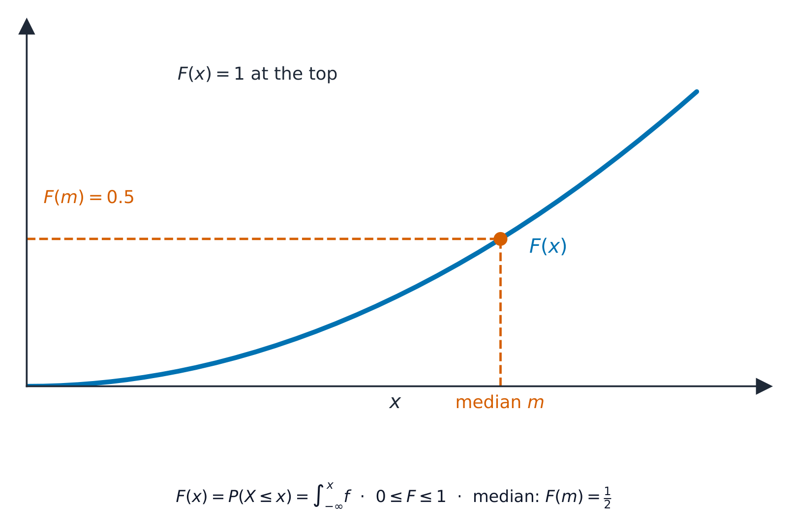
The cumulative distribution function 累积分布函数$F(x) = P(X \leqslant x)$ is the running total: $F(x) = \displaystyle\int_{-\infty}^{x} f(t)\,dt$, and $f(x) = F'(x)$. Use $F$ to find probabilities and percentiles 百分位数 (for example, the median 中位数 solves $F(x) = 0.5$).
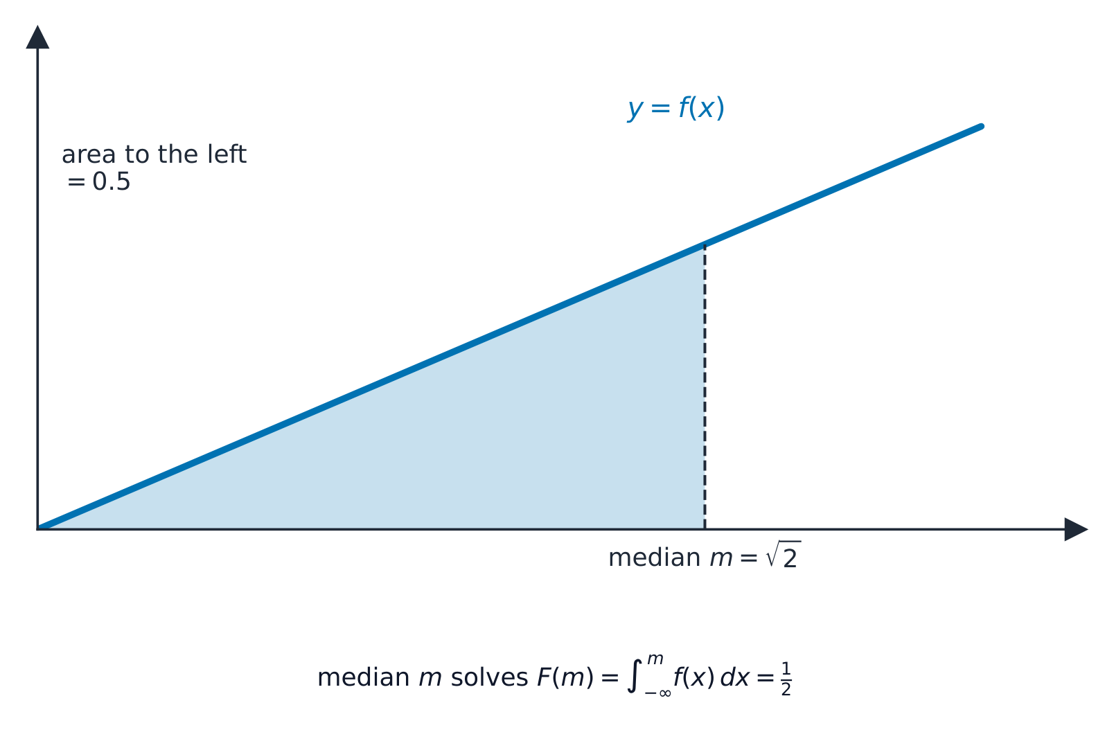
Worked example. A variable has $f(x) = \tfrac12 x$ for $0 \leqslant x \leqslant 2$. Find the median.
The cumulative distribution function is $F(x) = \displaystyle\int_0^x \tfrac12 t\,dt = \tfrac14 x^2$. Set $F(m) = 0.5$:
The distribution of a related variable. If $Y=g(X)$, find $Y$'s distribution through its cumulative function. For $Y=X^2$: $F_Y(y)=P(X^2\leqslant y)=P(-\sqrt y\leqslant X\leqslant\sqrt y)=F_X(\sqrt y)-F_X(-\sqrt y)$, then differentiate for $f_Y=F_Y'$. When $g$ is monotonic increasing there is a shortcut, $F_Y(y)=F_X\big(g^{-1}(y)\big)$.
Worked example. With $f_X(x)=\tfrac12 x$ on $[0,2]$ (so $F_X(x)=\tfrac14 x^2$), let $Y=X^2$. For $0\leqslant y\leqslant 4$, $F_Y(y)=F_X(\sqrt y)=\tfrac14 y$, so $f_Y(y)=F_Y'(y)=\tfrac14$ – that is, $Y$ is uniform on $[0,4]$.
Bahasa Indonesia
Variabel kontinu $X$ dijelaskan oleh fungsi kepadatan probabilitas$f(x)$, yang mungkin didefinisikan secara berselang-seling. Probabilitas dalam suatu rentang adalah area di bawah $f$, dan rata-rata dari setiap fungsi dari $X$ adalah
$$E(g(X)) = \int g(x)\,f(x)\,dx.$$
Median berada di mana area di bawah $f(x)$ di sebelah kirinya tepat $0.5$.
Fungsi distribusi kumulatif$F(x) = P(X \leqslant x)$ adalah total berjalan: $F(x) = \displaystyle\int_{-\infty}^{x} f(t)\,dt$, dan $f(x) = F'(x)$. Gunakan $F$ untuk menemukan probabilitas dan persentil (misalnya, median menyelesaikan $F(x) = 0.5$).
Graf kumulatif $F(x)$ naik dari $0$ ke $1$; ketinggian $0.5$ dicapai pada median.
Contoh terpecahkan. Sebuah variabel memiliki $f(x) = \tfrac12 x$ untuk $0 \leqslant x \leqslant 2$. Temukan median.
Fungsi distribusi kumulatif adalah $F(x) = \displaystyle\int_0^x \tfrac12 t\,dt = \tfrac14 x^2$. Tetapkan $F(m) = 0.5$:
Distribusi variabel terkait. Jika $Y=g(X)$, temukan distribusi $Y$ melalui fungsi kumulatifnya. Untuk $Y=X^2$: $F_Y(y)=P(X^2\leqslant y)=P(-\sqrt y\leqslant X\leqslant\sqrt y)=F_X(\sqrt y)-F_X(-\sqrt y)$, kemudian turunkan untuk $f_Y=F_Y'$. Ketika $g$ monoton naik terdapat jalan pintas, $F_Y(y)=F_X\big(g^{-1}(y)\big)$.
Contoh terpecahkan. Dengan $f_X(x)=\tfrac12 x$ pada $[0,2]$ (sehingga $F_X(x)=\tfrac14 x^2$), misalkan $Y=X^2$. Untuk $0\leqslant y\leqslant 4$, $F_Y(y)=F_X(\sqrt y)=\tfrac14 y$, sehingga $f_Y(y)=F_Y'(y)=\tfrac14$ – yaitu, $Y$ bersifat seragam pada $[0,4]$.
Explore · Jelajahi
Continuous random variables · Variabel acak kontinu
P(a < X < b) = ∫ f(x) dx
For a continuous variable, probability is the area under the density curve. · Untuk variabel kontinu, probabilitas adalah luas di bawah kurva densitas.
Inference using normal and t-distributions · Inferensi menggunakan distribusi normal dan t
Syllabus · Silabus
English
Candidates should be able to:
Notes and examples
formulate hypotheses and apply a hypothesis test concerning the population mean using a small sample drawn from a normal population of unknown variance, using a t-test
calculate a pooled estimate of a population variance from two samples
Calculations based on either raw or summarised data may be required.
formulate hypotheses concerning the difference of population means, and apply, as appropriate: - a 2-sample t-test - a paired sample t-test - a test using a normal distribution
The ability to select the test appropriate to the circumstances of a problem is expected.
determine a confidence interval for a population mean, based on a small sample from a normal population with unknown variance, using a t-distribution
determine a confidence interval for a difference of population means, using a t-distribution or a normal distribution, as appropriate.
Bahasa Indonesia
Calon peserta harus mampu:
Catatan dan contoh
susun hipotesis dan terapkan uji hipotesis mengenai rata-rata populasi menggunakan sampel kecil yang diambil dari populasi normal dengan variansi tak diketahui, menggunakan uji-t
hitung estimasi gabungan variansi populasi dari dua sampel
Perhitungan berdasarkan data mentah atau data yang diringkas mungkin diperlukan.
susun hipotesis mengenai perbedaan rata-rata populasi, dan terapkan, sesuai: - uji-t 2 sampel - uji-t sampel berpasangan - uji menggunakan distribusi normal
Kemampuan untuk memilih uji yang sesuai dengan situasi masalah diharapkan.
tentukan interval kepercayaan untuk rata-rata populasi, berdasarkan sampel kecil dari populasi normal dengan variansi tak diketahui, menggunakan distribusi-t
tentukan interval kepercayaan untuk perbedaan rata-rata populasi, menggunakan distribusi-t atau distribusi normal, sesuai.
Source: Cambridge International syllabus · Sumber: Silabus Cambridge International
English
When a sample is small and the population variance is unknown, base your hypothesis test 假设检验 on the $t$-distribution instead of the normal. The same idea gives a confidence interval 置信区间 for the mean:
$$\bar{x} \pm t\,\frac{s}{\sqrt{n}},$$
where $t$ comes from the $t$-tables with $n - 1$ degrees of freedom. To compare two populations, use a two-sample (2-sample) or paired-sample$t$-test, after finding a pooled estimate 合并估计 of the shared variance when appropriate.
Worked example. A sample of $n = 10$ has mean $\bar{x} = 50$ and standard deviation $s = 4$. Find a $95\%$ confidence interval for the mean (use $t = 2.262$ for $9$ degrees of freedom).
Papan Galton: bola jatuh melalui pin menumpuk menjadi distribusi normal berbentuk lonceng.
Ketika sampel kecil dan varians populasi tidak diketahui, dasar uji hipotesis Anda pada distribusi $t$ daripada normal. Ide yang sama memberikan interval kepercayaan untuk rata-rata:
$$\bar{x} \pm t\,\frac{s}{\sqrt{n}},$$
di mana $t$ berasal dari tabel $t$ dengan $n - 1$ derajat kebebasan. Untuk membandingkan dua populasi, gunakan uji-$t$dua-sampel (2-sampel) atau sampel berpasangan, setelah menemukan estimasi gabungan dari varians bersama yang sesuai.
Untuk sampel kecil distribusi $t$ lebih datar dengan ekor lebih tebal, sehingga nilai kritisnya lebih besar.
Contoh terpecahkan. Sebuah sampel $n = 10$ memiliki rata-rata $\bar{x} = 50$ dan simpangan baku $s = 4$. Temukan interval kepercayaan $95\%$ untuk rata-rata (gunakan $t = 2.262$ untuk derajat kebebasan $9$).
Why small samples need t instead of z · Mengapa sampel kecil membutuhkan t alih-alih z
With $\sigma$ unknown you use $t$, and $t$ has heavier tails than the normal (drawn dashed behind it) — so its critical values are larger and the interval is wider. At the worked example's $9$ degrees of freedom the widget reads $t^* = 2.262$, exactly the table value used above. Sweep df up and $t$ collapses onto the normal. · Dengan $\sigma$ yang tidak diketahui Anda menggunakan $t$, dan $t$ memiliki ekor lebih berat daripada normal (digambar putus-putus di belakangnya) — sehingga nilai kritisnya lebih besar dan intervalnya lebih lebar. Pada $9$ derajat kebebasan contoh terpecahkan, widget membaca $t^* = 2.262$, tepat nilai tabel yang digunakan di atas. Sweep df naik dan $t$ merapat ke normal.
Explore · Jelajahi
The normal distribution · Distribusi normal
Shade a tail to find a probability — the basis of confidence intervals and hypothesis tests. · Arsir ekor untuk menemukan probabilitas — dasar dari interval kepercayaan dan uji hipotesis.
4.3
Chi-squared tests · Uji chi-squared
Syllabus · Silabus
English
Candidates should be able to:
Notes and examples
fit a theoretical distribution, as prescribed by a given hypothesis, to given data
Questions will not involve lengthy calculations.
use a $\chi^2$-test, with the appropriate number of degrees of freedom, to carry out the corresponding goodness of fit analysis
Classes should be combined so that each expected frequency is at least 5.
use a $\chi^2$-test, with the appropriate number of degrees of freedom, for independence in a contingency table.
Yates’ correction is not required. Where appropriate, either rows or columns should be combined so that the expected frequency in each cell is at least 5.
Bahasa Indonesia
Calon peserta harus mampu:
Catatan dan contoh
sesuaikan distribusi teoritis, sesuai dengan hipotesis yang diberikan, pada data yang ada
Soal tidak akan melibatkan perhitungan yang panjang.
lakukan uji $\chi^2$, dengan jumlah derajat kebebasan yang sesuai, untuk melakukan analisis kesesuaian (goodness of fit) yang bersangkutan
Kelas harus digabungkan sedemikian rupa sehingga frekuensi harapan setiap kelas minimal 5.
lakukan uji $\chi^2$, dengan jumlah derajat kebebasan yang sesuai, untuk independensi dalam tabel kontingensi.
Koreksi Yates tidak diperlukan. Di mana perlu, baris atau kolom harus digabungkan sedemikian rupa sehingga frekuensi harapan di setiap sel minimal 5.
Source: Cambridge International syllabus · Sumber: Silabus Cambridge International
English
A $\chi^2$-test (chi-squared test 卡方检验) compares observed counts $O$ with expected counts $E$ from a theoretical distribution 理论分布:
$$\chi^2 = \sum \frac{(O - E)^2}{E}.$$
Compare this with a table value for the right number of degrees of freedom 自由度. Two uses: a goodness of fit 拟合优度 test (does the data follow the proposed model?), and a test for independence 独立性 of two variables in a contingency table 列联表.
Worked example. Four equally likely categories give observed counts $20, 30, 25, 25$ (so each expected count is $25$). Test the fit at the $5\%$ level.
With $4 - 1 = 3$ degrees of freedom the table value is $7.815$. Since $2 < 7.815$, do not reject the model.
Bahasa Indonesia
Uji $\chi^2$ (uji chi-kuadrat) membandingkan jumlah observasi $O$ dengan jumlah ekspektasi $E$ dari distribusi teoritis:
$$\chi^2 = \sum \frac{(O - E)^2}{E}.$$
Bandingkan ini dengan nilai tabel untuk jumlah derajat kebebasan yang benar. Dua penggunaan: uji kesesuaian (apakah data mengikuti model yang diusulkan?), dan uji ketergantungan dua variabel dalam tabel kontingensi.
Uji menolak model ketika $\chi^2$ melebihi nilai kritis, jatuh ke ekor diarsir $5\%$.
Contoh terpecahkan. Empat kategori yang setara kemungkinan memberikan jumlah observasi $20, 30, 25, 25$ (sehingga setiap jumlah ekspektasi adalah $25$). Uji kesesuaian pada tingkat $5\%$.
Dengan $4 - 1 = 3$ derajat kebebasan nilai tabel adalah $7.815$. Karena $2 < 7.815$, tolak model.
Explore · Jelajahi
The chi-squared distribution and its 5% tail · Distribusi chi-squared dan ekor 5%-nya
The worked example on this page gives $\chi^2 = 2$ with $3$ degrees of freedom against a table value of $7.815$ — the widget reproduces both. Drag df to see why the critical value changes with the number of categories. · Contoh terpecahkan di halaman ini memberikan $\chi^2 = 2$ dengan $3$ derajat kebebasan berbanding nilai tabel $7.815$ — widget mereproduksi keduanya. Seret df untuk melihat mengapa nilai kritis berubah dengan jumlah kategori.
Explore · Jelajahi
Chi-squared test route · Alur uji chi-squared
Follow observed and expected counts to a test decision. · Ikuti jumlah observasi dan ekspektasi menuju keputusan uji.
4.4
Non-parametric tests · Uji non-parametrik
Syllabus · Silabus
English
Candidates should be able to:
Notes and examples
understand the idea of a non-parametric test and appreciate situations in which such a test might be useful
e.g. when sampling from a population which cannot be assumed to be normally distributed.
understand the basis of the sign test, the Wilcoxon signed-rank test and the Wilcoxon rank-sum test
Including knowledge that Wilcoxon tests are valid only for symmetrical distributions.
use a single-sample sign test and a single-sample Wilcoxon signed-rank test to test a hypothesis concerning a population median
Including the use of normal approximations where appropriate. Questions will not involve tied ranks or observations equal to the population median value being tested.
use a paired-sample sign test, a Wilcoxon matched-pairs signed-rank test and a Wilcoxon rank-sum test, as appropriate, to test for identity of populations.
Including the use of normal approximations where appropriate. Questions will not involve tied ranks or zero‑difference pairs.
Bahasa Indonesia
Calon peserta harus mampu:
Catatan dan contoh
pahami konsep uji non-parametrik dan persepsi situasi di mana uji semacam itu mungkin berguna
mis. saat mengambil sampel dari populasi yang tidak dapat diasumsikan berdistribusi normal.
pahami dasar uji tanda, uji Wilcoxon signed-rank dan uji Wilcoxon rank-sum
Termasuk pengetahuan bahwa uji Wilcoxon hanya valid untuk distribusi simetris.
gunakan uji tanda satu sampel dan uji Wilcoxon signed-rank satu sampel untuk menguji hipotesis mengenai median populasi
Termasuk penggunaan pendekatan normal di mana perlu. Soal tidak akan melibatkan peringkat terikat atau observasi yang sama dengan nilai median populasi yang diuji.
gunakan uji tanda pasangan sampel, uji Wilcoxon matched-pairs signed-rank dan uji Wilcoxon rank-sum, secukupnya, untuk menguji kesamaan populasi.
Termasuk penggunaan pendekatan normal di mana perlu. Soal tidak akan melibatkan peringkat terikat atau pasangan dengan perbedaan nol.
Source: Cambridge International syllabus · Sumber: Silabus Cambridge International
English
A non-parametric test 非参数检验 makes no assumption that the data is normal, so it is useful when that assumption fails. The basic ones are:
the sign test 符号检验: count how many values fall above and below a proposed median, and test those counts with a binomial model;
the Wilcoxon signed-rank test 威尔科克森符号秩检验 (the matched-pairs test for paired data), which also uses the sizes of the differences, not just their signs;
the Wilcoxon rank-sum test 威尔科克森秩和检验, for comparing two separate samples.
Worked example. Test whether a median is $5$. In a sample of $10$ values (none equal to $5$), $9$ lie above$5$ and $1$ lies below. Test at the $5\%$ level (two-tailed).
Under $H_0$ (median $= 5$) the number above follows $B(10, 0.5)$. The observed result ($9$ above) is extreme, so find $P(X \geq 9) = \binom{10}{9}(0.5)^{10} + (0.5)^{10} = \dfrac{11}{1024} = 0.0107$. For a two-tailed test compare with $\tfrac{1}{2}(5\%) = 0.025$. Since $0.0107 < 0.025$, reject $H_0$: there is evidence the median is not $5$.
Bahasa Indonesia
Uji non-parametrik tidak mengasumsikan data berdistribusi normal, sehingga berguna ketika asumsi tersebut tidak terpenuhi. Uji dasar meliputi:
uji tanda: hitung berapa banyak nilai yang berada di atas dan di bawah median yang diusulkan, lalu uji jumlah tersebut dengan model binomial;
uji Wilcoxon bertanda-berperingkat (uji pasangan cocok untuk data berpasangan), yang juga menggunakan besaran selisihnya, bukan hanya tandanya;
uji Wilcoxon penjumlahan peringkat, untuk membandingkan dua sampel terpisah.
Uji tanda menghitung berapa banyak nilai yang berada di atas dan di bawah median yang diusulkan, kemudian menguji jumlah tersebut dengan model binomial
Contoh terpecahkan. Uji apakah sebuah median adalah $5$. Dalam sampel $10$ nilai (tidak ada yang sama dengan $5$), $9$ terletak di atas$5$ dan $1$ terletak di bawahnya. Ujilah pada tingkat $5\%$ (dua sisi).
Di bawah $H_0$ (median $= 5$) jumlah nilai di atas mengikuti $B(10, 0.5)$. Hasil yang diamati ($9$ di atas) bersifat ekstrem, sehingga cari $P(X \geq 9) = \binom{10}{9}(0.5)^{10} + (0.5)^{10} = \dfrac{11}{1024} = 0.0107$. Untuk uji dua sisi, bandingkan dengan $\tfrac{1}{2}(5\%) = 0.025$. Karena $0.0107 < 0.025$, tolak $H_0$: terdapat bukti bahwa median bukan $5$.
Explore · Jelajahi
Non-parametric test chooser · Pemilih uji non-parametrik
Choose the rank-based test that matches the data situation. · Pilih uji berbasis peringkat yang sesuai dengan situasi data.
probability generating function/ˌprɒbəˈbɪlɪti ˈdʒenəreɪtɪŋ ˈfʌŋkʃn/
fungsi pembangkit peluang
Further Probability & Statistics/ˈfɜːðə ˌprɒbəˈbɪlɪti ænd stəˈtɪstɪks/
Probabilitas & Statistik Lanjutan
4.5
Probability generating functions · Fungsi pembangkit peluang
Syllabus · Silabus
English
Candidates should be able to:
Notes and examples
understand the concept of a probability generating function (PGF) and construct and use the PGF for given distributions
Including the discrete uniform, binomial, geometric and Poisson distributions.
use formulae for the mean and variance of a discrete random variable in terms of its PGF, and use these formulae to calculate the mean and variance of a given probability distribution
use the result that the PGF of the sum of independent random variables is the product of the PGFs of those random variables.
Bahasa Indonesia
Calon peserta harus mampu:
Catatan dan contoh
pahami konsep fungsi pembangkit peluang (PGF) dan susun serta gunakan PGF untuk distribusi yang diberikan
Termasuk distribusi seragam diskrit, binomial, geometrik, dan Poisson.
gunakan rumus untuk rata-rata dan varians variabel acak diskrit dalam bentuk PGF-nya, dan gunakan rumus-rumus ini untuk menghitung rata-rata dan varians dari suatu distribusi peluang yang diberikan
gunakan hasil bahwa PGF dari jumlah variabel acak independen adalah hasil kali PGF dari variabel-variabel acak tersebut.
Source: Cambridge International syllabus · Sumber: Silabus Cambridge International
English
The probability generating function 概率母函数 of a discrete variable $X$ is
$$G(t) = E(t^X) = \sum_x P(X = x)\,t^x.$$
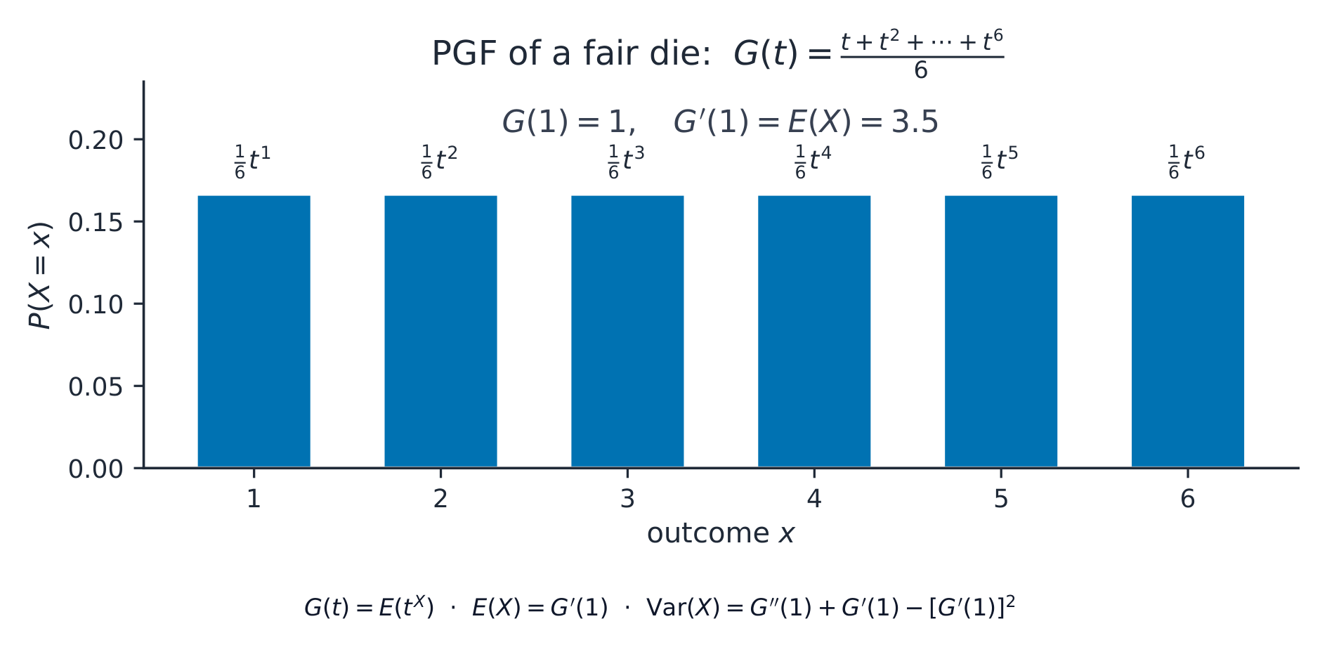
It packs the whole distribution into one function. The mean and variance come from its derivatives at $t = 1$: $E(X) = G'(1)$ and $\mathrm{Var}(X) = G''(1) + G'(1) - \big(G'(1)\big)^2$. Also, the PGF of a sum of independent variables is the product of their PGFs.
Worked example.$X$ has $P(X=0) = 0.5$, $P(X=1) = 0.3$, $P(X=2) = 0.2$. Find $E(X)$ using the PGF.
Here $G(t) = 0.5 + 0.3t + 0.2t^2$, so $G'(t) = 0.3 + 0.4t$ and
$$E(X) = G'(1) = 0.3 + 0.4 = 0.7.$$
Bahasa Indonesia
Dadu: titik awal untuk probabilitas dan variabel acak diskrit.
Fungsi pembangkit peluang dari variabel diskrit $X$ adalah
$$G(t) = E(t^X) = \sum_x P(X = x)\,t^x.$$
Fungsi ini memadatkan seluruh distribusi ke dalam satu fungsi. Rata-rata dan varians diperoleh dari turunannya di $t = 1$: $E(X) = G'(1)$ dan $\mathrm{Var}(X) = G''(1) + G'(1) - \big(G'(1)\big)^2$. Selain itu, PGF dari penjumlahan variabel independen adalah hasil kali PGF masing-masing variabel.
Contoh terpecahkan.$X$ memiliki $P(X=0) = 0.5$, $P(X=1) = 0.3$, $P(X=2) = 0.2$. Temukan $E(X)$ menggunakan PGF.
Di sini $G(t) = 0.5 + 0.3t + 0.2t^2$, sehingga $G'(t) = 0.3 + 0.4t$ dan
$$E(X) = G'(1) = 0.3 + 0.4 = 0.7.$$
PGF dadu adil memadatkan massa yang sama pada angka 1 hingga 6 ke dalam G(t)
Explore · Jelajahi
Probability generating function lab · Laboratorium fungsi pembangkit peluang
G(x) = p0 + p1 x + p2 x^2 + ...
Change x and see how a PGF stores probabilities in powers of x. · Ubah x dan lihat bagaimana PGF menyimpan peluang dalam pangkat x.
4.5
Exam tips · Tips ujian
English
For a continuous random variable, the pdf integrates to $1$ over its range, and $E(X) = \int x f(x)\,dx$.
Use the $t$-distribution when the sample is small and the population variance is unknown; state the degrees of freedom.
For a chi-squared test compute $\sum (O-E)^2/E$, compare with the critical value at the right degrees of freedom, and combine classes with $E < 5$.
State $H_0$ and $H_1$ and give the conclusion in context for every test.
Bahasa Indonesia
Untuk variabel acak kontinu, pdf terintegrasi menjadi $1$ sepanjang rentangnya, dan $E(X) = \int x f(x)\,dx$.
Gunakan distribusi-$t$ jika sampel kecil dan varians populasi tidak diketahui; nyatakan derajat kebebasannya.
Untuk uji chi-squared hitung $\sum (O-E)^2/E$, bandingkan dengan nilai kritis pada derajat kebebasan yang sesuai, dan gabungkan kelas dengan $E < 5$.
Nyatakan $H_0$ dan $H_1$ serta berikan kesimpulan dalam konteks untuk setiap uji.
Interactive lessons on this topic · Pelajaran interaktif untuk topik ini
Work through it step by step, with instant-check exercises. · Kerjakan langkah demi langkah, dengan latihan pengecekan instan.
More topics in A-Level Further Mathematics · Matematika Lanjutan A-Level · Topik lain dalam A-Level Further Mathematics · Matematika Lanjutan A-Level
Pick one and the site follows you — notes, papers, videos and practice all open on it. · Pilih satu dan situs mengikuti Anda — catatan, kertas, video, dan latihan semua terbuka di sana.
Type to search notes, lessons, code, vocabulary and past-paper questions across every subject. · Ketik untuk mencari catatan, pelajaran, kode, kosakata, dan pertanyaan soal lama di setiap mata pelajaran.