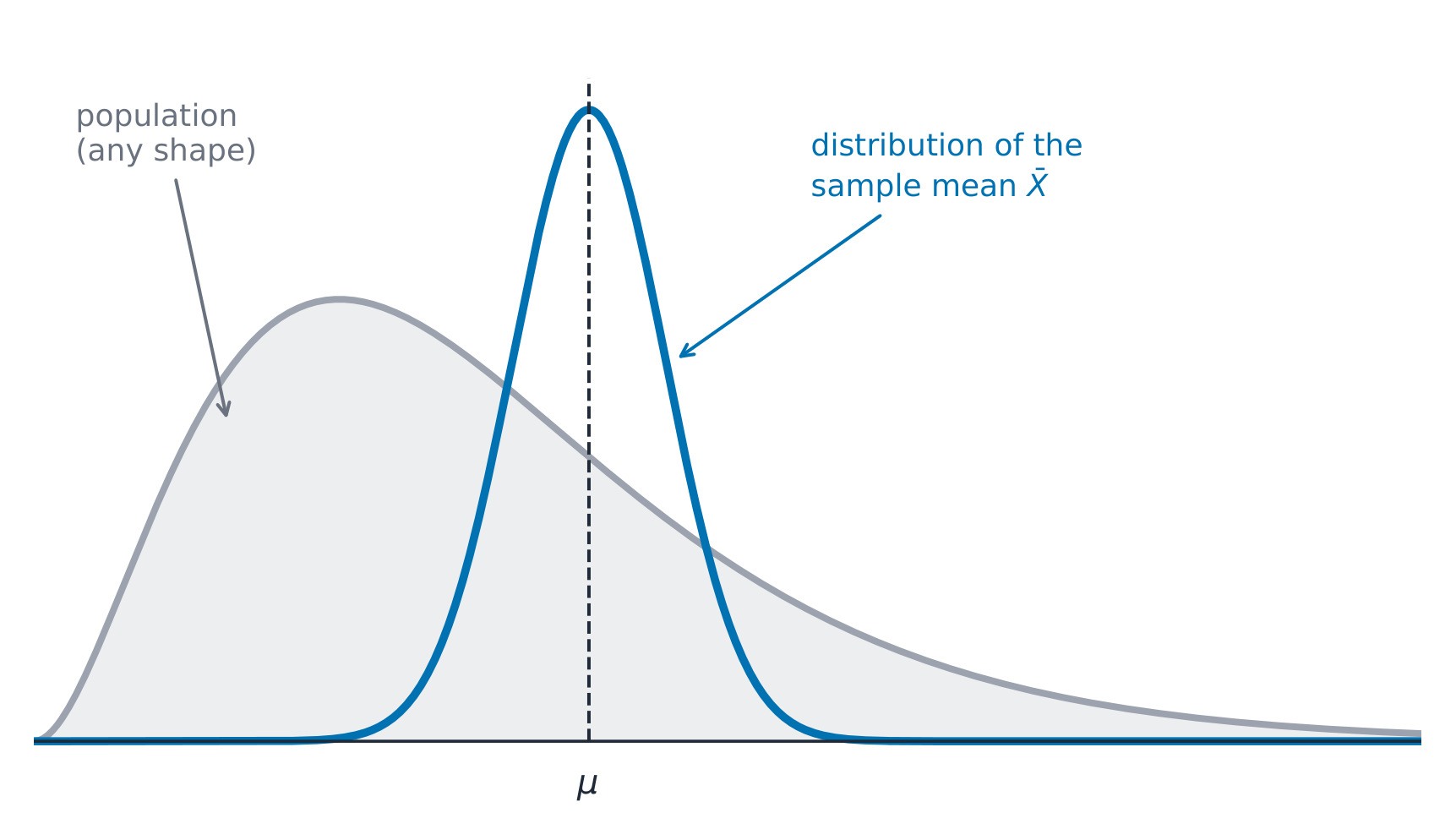
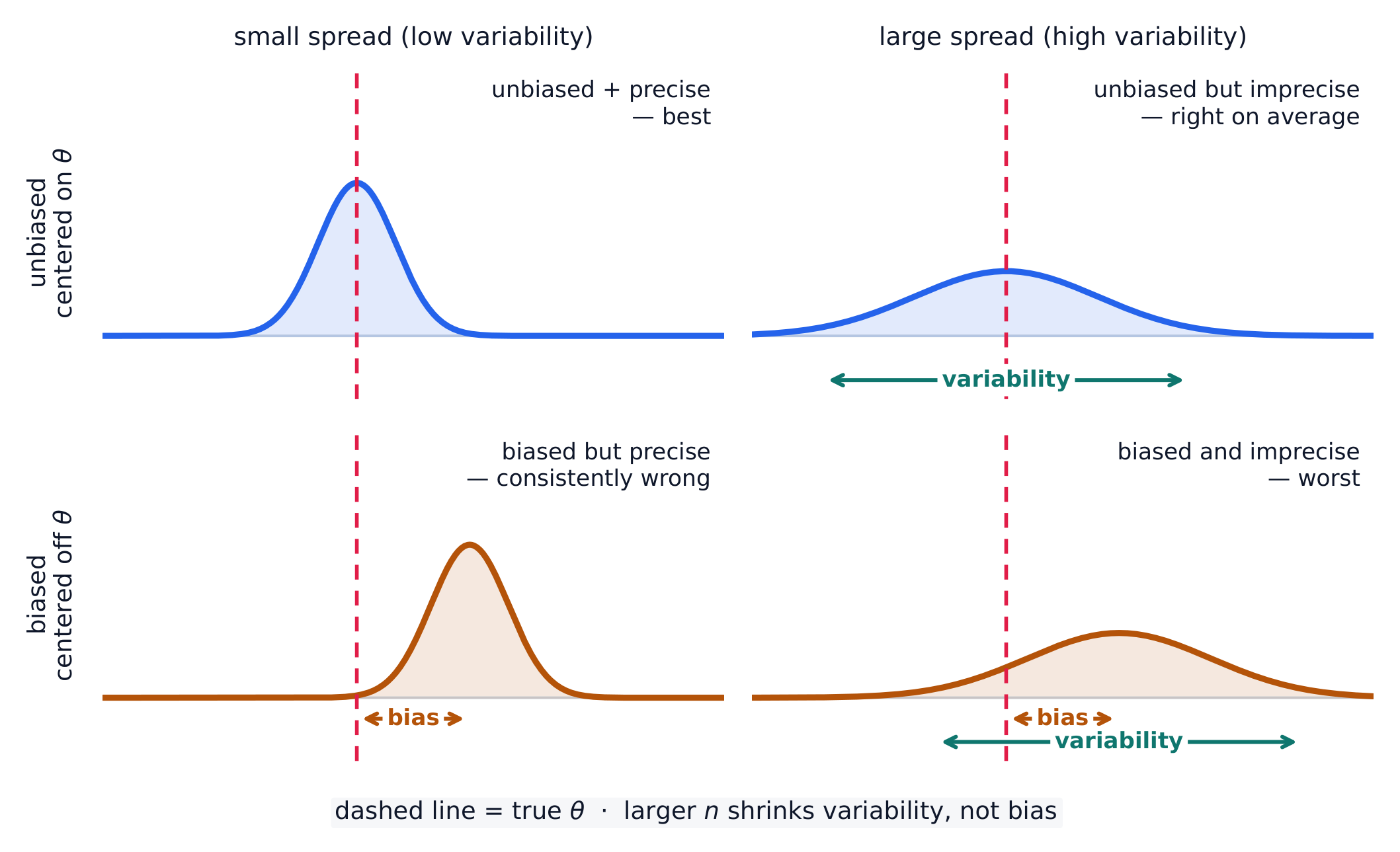
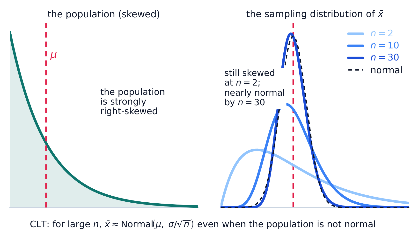
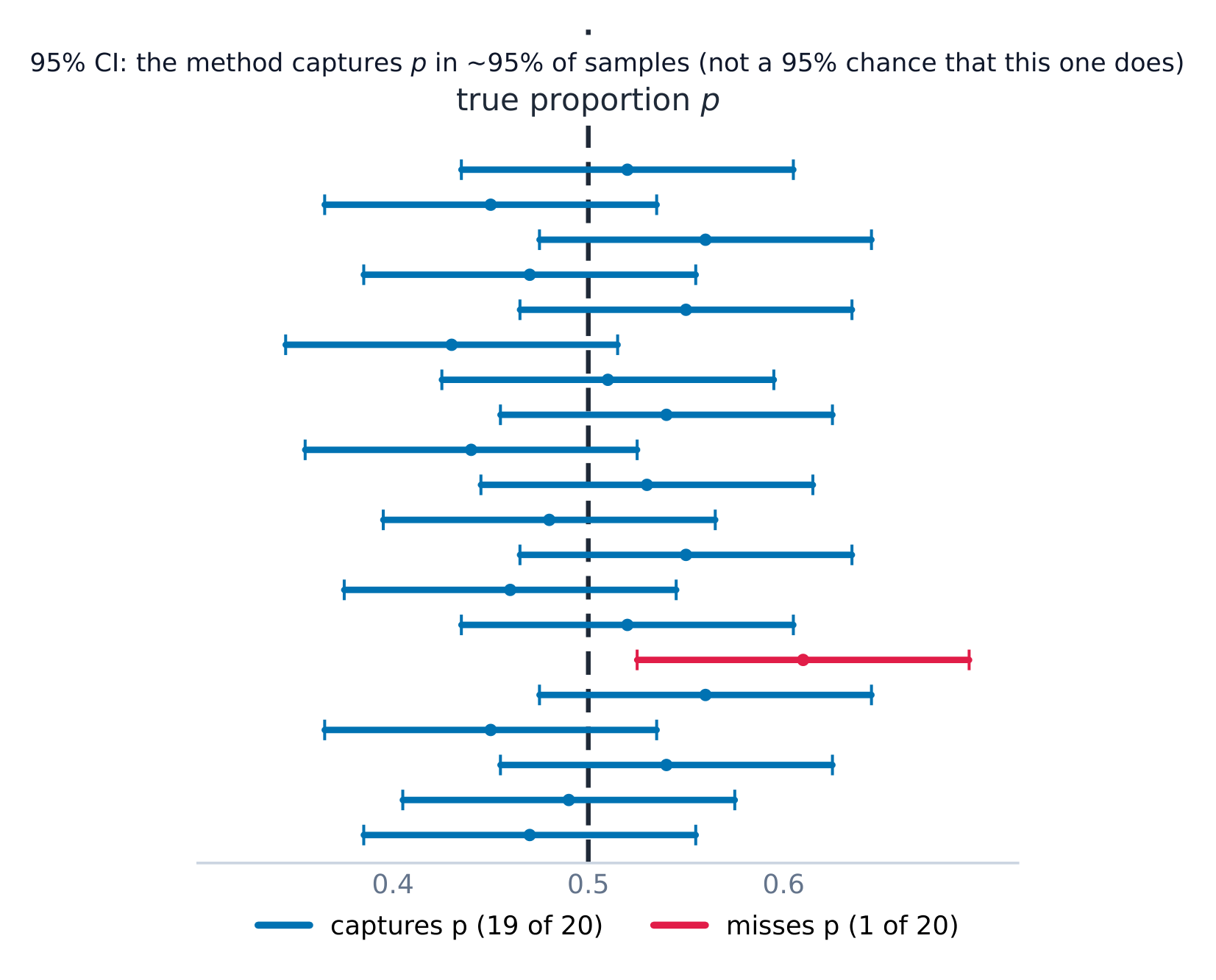
يغطي إحصاء AP استكشاف البيانات، والتجارب والتخطيط التجريبي، والاحتمالات والمتغيرات العشوائية، وتوزيعات العينات، والاستدلال الإحصائي—بما في ذلك فترات الثقة واختبارات الدلالة. لا يوجد الكثير من الجبر؛ الصعوبة تكمن في صياغة التصريح الصحيح حول عدم اليقين.
كل إجابة استدلال تتكون من أربعة أجزاء: تحديد الإجراء، وفحص الشروط، والحساب، والاستنتاج في السياق مع الربط بافتراض البديل. يتم تقييم جميع الأجزاء الأربعة حسب مقياس الدرجات، لذا فإن الحصول على قيمة p صحيحة وحدها لا يكفي للحصول على درجة جيدة.
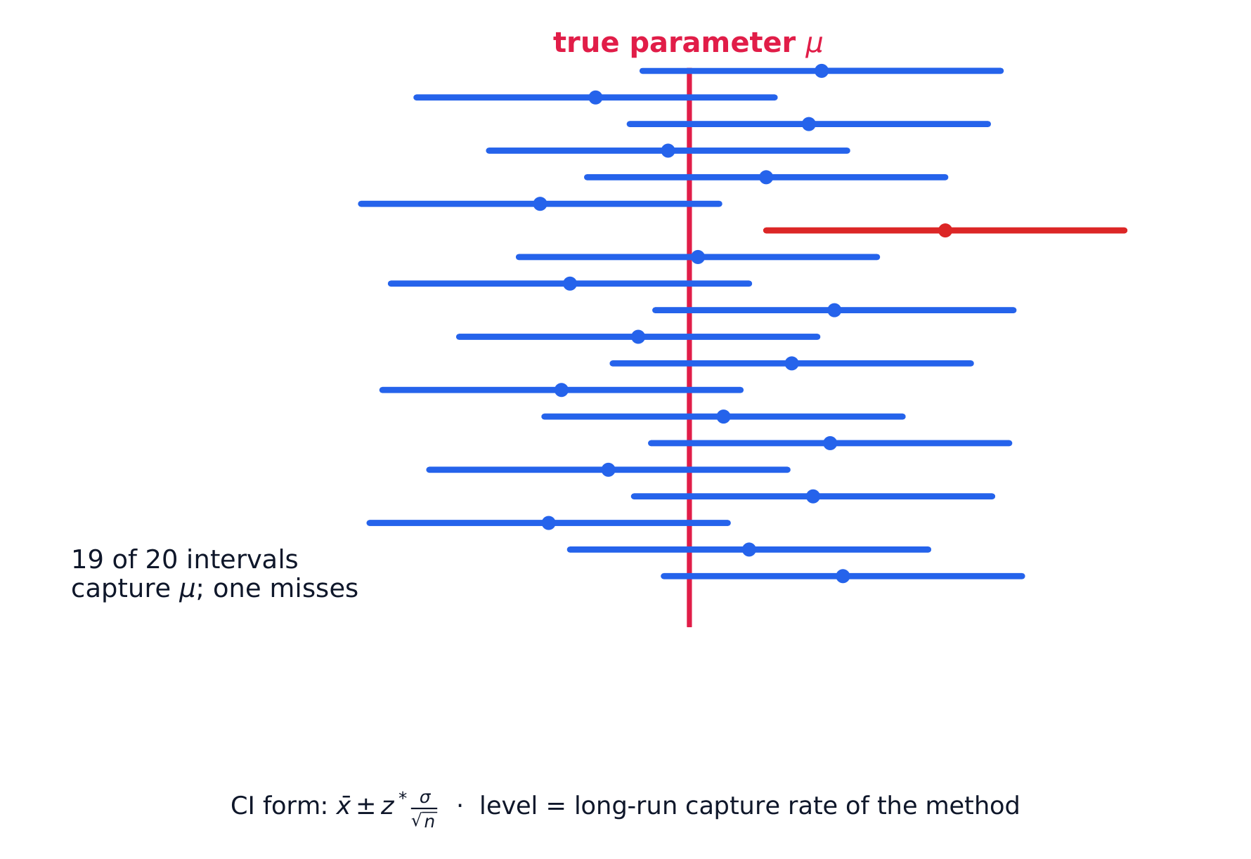
اللغة محل تقييم. "نرفض H₀" ليست "نثبت H₁"؛ فترة الثقة تتعلق بـسلوك الطريقة على المدى الطويل، وليس احتمال أن تحتوي فترة معينة على المعامل. هذه التمييزات تحدد الدرجات.
تعتمد الملاحظات على جميع الوحدات التسع مع وضع كل إجراء استدلالي خطوة بخطوة. الاختبارات الحرة (FRQs) المنشورة متوفرة في المكتبة. يمنح الإحصاء درجات لـتوضيح الشروط والتفسير في السياق، لذلك يُذكر كل حل نموذجي الشروط قبل إجراء الاختبار.
Introducing Statistics: What Can We Learn from Data? · مقدمة الإحصاء: ماذا يمكننا تعلمه من البيانات؟
Syllabus · المنهج
English
Enduring Understanding (VAR-1): Given that variation may be random or not, conclusions are uncertain.
Learning Objective VAR-1.A: Identify questions to be answered, based on variation in one-variable data. [Skill 1.A]
VAR-1.A.1 Numbers may convey meaningful information, when placed in context.
العربية
الفهم الدائم (VAR-1): بما أن التباين قد يكون عشوائياً أو غير ذلك، فإن الاستنتاجات تكون غير مؤكدة.
هدف التعلم VAR-1.A: تحديد الأسئلة المراد الإجابة عليها، بناءً على تباين بيانات متغير واحد. [مهارة 1.A]
VAR-1.A.1 قد تحمل الأرقام معلومات ذات معنى، عند وضعها في سياق.
Source: College Board AP Course and Exam Description · المصدر: وصف دورة وامتحان College Board AP
English
Statistics 统计学 is the science of learning from data 数据 – numbers or labels collected from the real world. Data vary, so we describe patterns and account for the variation 变异 rather than expecting every value to match. A statistical question anticipates an answer based on data that vary.
Two distinctions run through the whole course. A parameter 参数 is a numerical summary of a whole population; a statistic 统计量 is a numerical summary of a sample - we use the statistic to estimate the parameter we cannot measure directly. And descriptive statistics 描述统计 only summarise the data set in hand, while inferential statistics 推断统计 use a sample to make and test claims about the larger population.
العربية
الإحصاء هو علم التعلم من البيانات – الأرقام أو العلامات المجمعة من العالم الحقيقي. تتفاوت البيانات، لذا نصف الأنماط ونأخذ في الاعتبار التفاوت بدلاً من توقع مطابقة كل قيمة. السؤال الإحصائي يتوقع إجابة بناءً على بيانات متفاوتة.
يمر تمييزان عبر المقرر بأكمله. المعامل هو ملخص رقمي لـ مجتمع كامل؛ والإحصاء هو ملخص رقمي لـ عينة - نستخدم الإحصاء لتقدير المعامل الذي لا يمكننا قياسه مباشرة. والإحصاء الوصفي يلخص فقط مجموعة البيانات المتاحة، بينما الإحصاء الاستدلالي يستخدم العينة لإثبات واختبار ادعاءات حول المجتمع الأكبر.
1.2
The Language of Variation: Variables · لغة التفاوت: المتغيرات
Syllabus · المنهج
English
Enduring Understanding (VAR-1): Given that variation may be random or not, conclusions are uncertain.
Learning Objective VAR-1.B: Identify variables in a set of data. [Skill 2.A]
VAR-1.B.1 A variable is a characteristic that changes from one individual to another.
Learning Objective VAR-1.C: Classify types of variables. [Skill 2.A]
VAR-1.C.1 A categorical variable takes on values that are category names or group labels.
VAR-1.C.2 A quantitative variable is one that takes on numerical values for a measured or counted quantity.
Illustrative examples for VAR-1.C:
Categorical variables:
Dominant hand
Age group (young or old)
Highest degree earned
Quantitative variables:
Age of a structure
Height of a child
Concentration of a sample
العربية
الفهم الدائم (VAR-1): بما أن التباين قد يكون عشوائياً أو غير ذلك، فإن الاستنتاجات تكون غير مؤكدة.
هدف التعلم VAR-1.B: تحديد المتغيرات في مجموعة بيانات. [مهارة 2.A]
VAR-1.B.1 المتغير هو سمة تتغير من فرد إلى آخر.
هدف التعلم VAR-1.C: تصنيف أنواع المتغيرات. [مهارة 2.A]
VAR-1.C.1 المتغير التصنيفي يأخذ قيماً هي أسماء فئات أو تسميات مجموعات.
VAR-1.C.2 المتغير الكمي هو الذي يأخذ قيماً رقمية لكمية مقاسة أو معدودة.
أمثلة توضيحية لـ VAR-1.C:
المتغيرات التصنيفية:
اليد السائدة
فئة العمر (صغير أو كبير)
أعلى شهادة تم الحصول عليها
المتغيرات الكمية:
عمر بنية ما
طول طفل
تركيز عينة ما
Source: College Board AP Course and Exam Description · المصدر: وصف دورة وامتحان College Board AP
English
A variable 变量 is a characteristic that can differ between individuals. Two kinds:
Categorical 分类 (qualitative): values are labels/groups (eye colour, brand).
Quantitative 定量: values are numbers you can do arithmetic on (height, age). Quantitative variables are discrete (countable) or continuous (measured).
Choosing the right graph and summary depends on which kind you have.
العربية
المتغير هو خاصية يمكن أن تختلف بين الأفراد. نوعان:
تصنيفي (نوعي): القيم هي علامات/مجموعات (لون العين، العلامة التجارية).
كمّي: القيم هي أرقام يمكنك إجراء عمليات حسابية عليها (الطول، العمر). المتغيرات الكمية منفصلة (قابلة للعد) أو متصلة (مقاسة).
يعتمد اختيار الرسم البياني والملخص المناسب على النوع الذي لديك.
Explore · استكشف
Categorical or quantitative? · فئة أم كمي؟
Every variable is either categorical (it labels each unit with a group) or quantitative (a measured number you can average). Which kind it is decides the graphs and summaries you are allowed to use. · كل متغير إما فئة (يُصنّف كل وحدة في مجموعة) أو كمّي (رقم مقاس يمكن حساب متوسطه). نوعه يحدد الرسوم البيانية والملخصات المسموح باستخدامها.
1.3
Representing a Categorical Variable with Tables · تمثيل متغير تصنيفي بجداول
Syllabus · المنهج
English
Enduring Understanding (UNC-1): Graphical representations and statistics allow us to identify and represent key features of data.
Learning Objective UNC-1.A: Represent categorical data using frequency or relative frequency tables. [Skill 2.B]
UNC-1.A.1 A frequency table gives the number of cases falling into each category. A relative frequency table gives the proportion of cases falling into each category.
Learning Objective UNC-1.B: Describe categorical data represented in frequency or relative tables. [Skill 2.A]
UNC-1.B.1 Percentages, relative frequencies, and rates all provide the same information as proportions.
UNC-1.B.2 Counts and relative frequencies of categorical data reveal information that can be used to justify claims about the data in context.
العربية
الفهم الدائم (UNC-1): تُمكّننا التمثيلات البيانية والإحصاءات من تحديد وميزة الملامح الرئيسية للبيانات.
هدف التعلم UNC-1.A: تمثيل البيانات الفئوية باستخدام جداول التكرار أو التكرار النسبي. [مهارة 2.B]
UNC-1.A.1 تعطي جدول التكرار عدد الحالات التي تندرج تحت كل فئة. بينما يعطي جدول التكرار النسبي نسبة الحالات التي تندرج تحت كل فئة.
هدف التعلم UNC-1.B: وصف البيانات الفئوية الممثلة في جداول التكرار أو النسب. [مهارة 2.A]
UNC-1.B.1 تقدم النسب المئوية والتكرارات النسبية والمعدلات نفس المعلومات كالنسب.
UNC-1.B.2 تكشف أعداد وتكرارات النسب للبيانات الفئوية عن معلومات يمكن استخدامها لتبرير الادعاءات حول البيانات في سياقها.
Source: College Board AP Course and Exam Description · المصدر: وصف دورة وامتحان College Board AP
English
A frequency table 频数表 lists each category's count (frequency); a relative frequency 相对频率 table lists each category's proportion 比例 (count ÷ total). Relative frequencies let you compare groups of different sizes fairly.
العربية
جدول التواتر يعدّ عدد (تردد) كل فئة؛ وجدول التواتر النسبي يعدّ نسبة (عدد ÷ إجمالي) كل فئة. تتيح التواترات النسبية مقارنة مجموعات ذات أحجام مختلفة بشكل عادل.
1.4
Representing a Categorical Variable with Graphs · تمثيل متغير تصنيفي برسومات بيانية
Syllabus · المنهج
English
Enduring Understanding (UNC-1): Graphical representations and statistics allow us to identify and represent key features of data.
Learning Objective UNC-1.C: Represent categorical data graphically. [Skill 2.B]
UNC-1.C.1 Bar charts (or bar graphs) are used to display frequencies (counts) or relative frequencies (proportions) for categorical data.
UNC-1.C.2 The height or length of each bar in a bar graph corresponds to either the number or proportion of observations falling within each category.
UNC-1.C.3 There are many additional ways to represent frequencies (counts) or relative frequencies (proportions) for categorical data.
Learning Objective UNC-1.D: Describe categorical data represented graphically. [Skill 2.A]
UNC-1.D.1 Graphical representations of a categorical variable reveal information that can be used to justify claims about the data in context.
UNC-1.E.1 Frequency tables, bar graphs, or other representations can be used to compare two or more data sets in terms of the same categorical variable.
العربية
الفهم الدائم (UNC-1): تُمكّننا التمثيلات البيانية والإحصاءات من تحديد وميزة الملامح الرئيسية للبيانات.
هدف التعلم UNC-1.C: تمثيل البيانات الفئوية بيانياً. [مهارة 2.B]
UNC-1.C.1 تُستخدم الرسوم البيانية الشريطية (أو مخططات الأشرطة) لعرض التكرارات (الأعداد) أو التكرارات النسبية (النسب) للبيانات الفئوية.
UNC-1.C.2 يتوافق ارتفاع أو طول كل شريط في الرسم البياني الشريطي إما مع عدد أو نسبة الملاحظات التي تندرج ضمن كل فئة.
UNC-1.C.3 توجد طرق إضافية عديدة لتمثيل التكرارات (الأعداد) أو التكرارات النسبية (النسب) للبيانات الفئوية.
هدف التعلم UNC-1.D: وصف البيانات الفئوية الممثلة بيانياً. [مهارة 2.A]
UNC-1.D.1 تكشف التمثيلات البيانية للمتغير الفئي عن معلومات يمكن استخدامها لتبرير الادعاءات حول البيانات في سياقها.
هدف التعلم UNC-1.E: مقارنة مجموعات متعددة من البيانات الفئوية. [مهارة 2.D]
UNC-1.E.1 يمكن استخدام جداول التكرار أو الرسوم البيانية الشريطية أو غيرها من التمثيلات لمقارنة مجموعتين أو أكثر من مجموعات البيانات من حيث نفس المتغير الفئي.
Source: College Board AP Course and Exam Description · المصدر: وصف دورة وامتحان College Board AP
English
Bar charts 条形图 show the count or proportion of each category as separated bars; a pie chart shows each category's share of the whole. The bar heights (or slices) let you compare categories at a glance. Bars may be ordered by size or by a natural category order.
العربية
المخططات الشريطية تُظهر عدد أو نسبة كل فئة كأشرطة منفصلة؛ والمخطط الدائري يُظهر حصة كل فئة من الكل. تسمح ارتفاعات الأشرطة (أو المقاطع) بمقارنة الفئات بنظرة سريعة. قد تكون الأشرطة مرتبة حسب الحجم أو حسب ترتيب فئوي طبيعي.
Explore · استكشف
Show a categorical variable as a pie chart · اعرض متغيراً فئياً كمخطط دائري
A pie chart turns each category's share of the whole into a slice: a bigger share is a bigger slice, and every slice together makes 100%. It is a picture of a relative-frequency table. · المخطط الدائري يحول نسبة كل فئة من الكل إلى قطعة: النسبة الأكبر تعني قطعة أكبر، وكل القطع معاً تشكل 100%. إنه صورة لجدول تردد نسبي.
1.5
Representing a Quantitative Variable with Graphs · تمثيل متغير كمّي برسومات بيانية
Syllabus · المنهج
English
Enduring Understanding (UNC-1): Graphical representations and statistics allow us to identify and represent key features of data.
Learning Objective UNC-1.F: Classify types of quantitative variables. [Skill 2.A]
UNC-1.F.1 A discrete variable can take on a countable number of values. The number of values may be finite or countably infinite, as with the counting numbers.
UNC-1.F.2 A continuous variable can take on infinitely many values, but those values cannot be counted. No matter how small the interval between two values of a continuous variable, it is always possible to determine another value between them.
Illustrative examples for UNC-1.F:
A discrete variable:
Number of students in a class
A continuous variable:
Height of a child
Learning Objective UNC-1.G: Represent quantitative data graphically. [Skill 2.B]
UNC-1.G.1 In a histogram, the height of each bar shows the number or proportion of observations that fall within the interval corresponding to that bar. Altering the interval widths can change the appearance of the histogram.
UNC-1.G.2 In a stem and leaf plot, each data value is split into a "stem" (the first digit or digits) and a "leaf" (usually the last digit).
UNC-1.G.3 A dotplot represents each observation by a dot, with the position on the horizontal axis corresponding to the data value of that observation, with nearly identical values stacked on top of each other.
UNC-1.G.4 A cumulative graph represents the number or proportion of a data set less than or equal to a given number.
UNC-1.G.5 There are many additional ways to graphically represent distributions of quantitative data.
العربية
الفهم الدائم (UNC-1): تُمكّننا التمثيلات البيانية والإحصاءات من تحديد وميزة الملامح الرئيسية للبيانات.
هدف التعلم UNC-1.F: تصنيف أنواع المتغيرات الكمية. [مهارة 2.A]
UNC-1.F.1 يمكن للمتغير المنفصل أن يأخذ عدداً قابلاً للعد من القيم. قد يكون عدد القيم محدوداً أو لا نهائياً قابلاً للعد، كما هو الحال مع أعداد العد.
UNC-1.F.2 يمكن للمتغير المستمر أن يأخذ عدداً لا نهائياً من القيم، ولكن لا يمكن عد تلك القيم. بغض النظر عن مدى صغر الفترة الزمنية بين قيمتين لمتغير مستمر، يكون دائماً من الممكن تحديد قيمة أخرى بينهما.
أمثلة توضيحية لـ UNC-1.F:
متغير منفصل:
عدد الطلاب في فصل دراسي
متغير مستمر:
طول طفل
هدف التعلم UNC-1.G: تمثيل البيانات الكمية بيانياً. [مهارة 2.B]
UNC-1.G.1 في المدرج التكراري، يُظهر ارتفاع كل شريط عدد أو نسبة الملاحظات التي تندرج ضمن الفترة المقابلة لذلك الشريط. تغيير عرض الفترات يمكن أن يغير مظهر المدرج التكراري.
UNC-1.G.2 في مخطط الجذع والأوراق، يتم تقسيم كل قيمة بيانات إلى "جذع" (الرقم الأول أو الأرقام الأولى) و"ورقة" (عادة الرقم الأخير).
UNC-1.G.3 يمثل المخطط النقطي كل ملاحظة بنقطة، حيث تتوافق الموقع على المحور الأفقي مع قيمة البيانات الخاصة بتلك الملاحظة، مع تراكم القيم المتطابقة تقريباً فوق بعضها البعض.
UNC-1.G.4 يمثل الرسم التراكمي عدد أو نسبة مجموعة البيانات الأقل من أو يساوي رقماً معيناً.
UNC-1.G.5 توجد طرق إضافية عديدة لتمثيل التوزيعات للبيانات الكمية بيانياً.
Source: College Board AP Course and Exam Description · المصدر: وصف دورة وامتحان College Board AP
English
For numbers, use a dotplot 点图, stem-and-leaf plot 茎叶图, or histogram 直方图 (bars over value intervals called bins). These show the distribution 分布 – how the values spread out. A histogram's bin width changes the picture, so choose it to reveal the shape.
العربية
للأرقام، استخدم المخطط النقطي، أو مخطط الساق والورقة، أو المخطط التكراري (أشرطة فوق فترات قيمة تسمى صناديق). تُظهر هذه الـتوزيع – كيف تنتشر القيم. يغير عرض صندوق المخطط التكراري الصورة، لذا اختره لكشف الشكل.
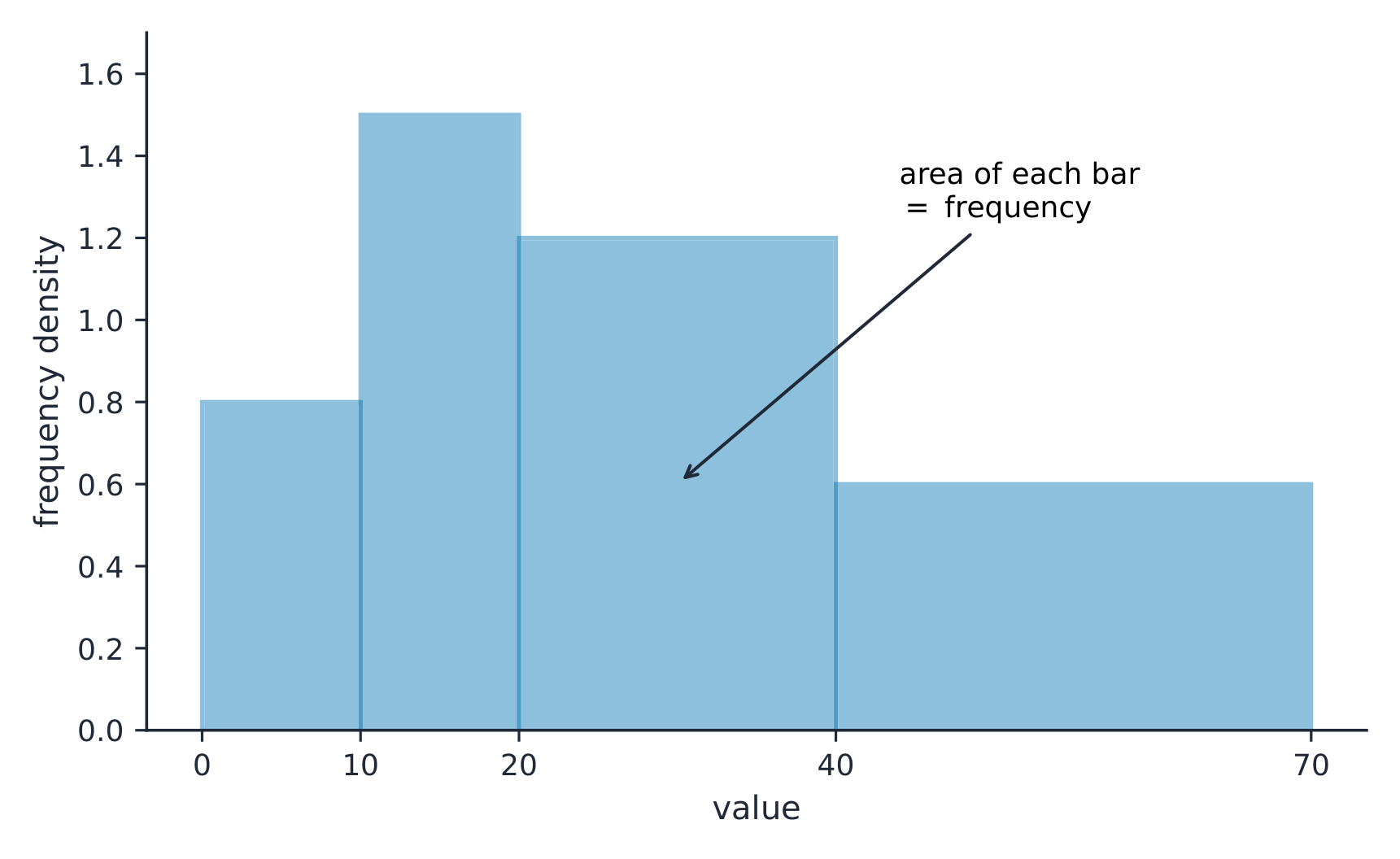
على المخطط التكراري ذو العرض غير المتساوٍ للفئات، مساحة الشريط هي التواتر
Explore · استكشف
Explore how bin width shapes a histogram · استكشف كيف يؤثر عرض الشريط على شكل المدرجة التكرارية
A histogram groups data into equal-width bins and draws a bar over each. Change the bins and notice how the same data can look jagged (too narrow) or smooth (too wide) — the shape is a choice. · المدرجة التكرارية تجمع البيانات في شرائط متساوية العرض وترسم عموداً فوق كل شريط. غيّر الشرائط ولاحظ كيف يمكن أن تبدو نفس البيانات متعرجة (ضيقة جداً) أو سلسة (واسعة جداً) — الشكل اختيار.
Describing the Distribution of a Quantitative Variable · وصف توزيع متغير كمّي
Syllabus · المنهج
English
Enduring Understanding (UNC-1): Graphical representations and statistics allow us to identify and represent key features of data.
Learning Objective UNC-1.H: Describe the characteristics of quantitative data distributions. [Skill 2.A]
UNC-1.H.1 Descriptions of the distribution of quantitative data include shape, center, and variability (spread), as well as any unusual features such as outliers, gaps, clusters, or multiple peaks.
UNC-1.H.2 Outliers for one-variable data are data points that are unusually small or large relative to the rest of the data.
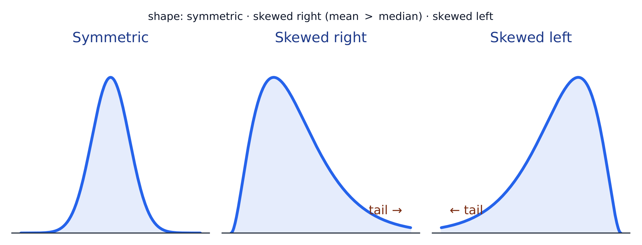
UNC-1.H.3 A distribution is skewed to the right (positive skew) if the right tail is longer than the left. A distribution is skewed to the left (negative skew) if the left tail is longer than the right. A distribution is symmetric if the left half is the mirror image of the right half.
UNC-1.H.4 Univariate graphs with one main peak are known as unimodal. Graphs with two prominent peaks are bimodal. A graph where each bar height is approximately the same (no prominent peaks) is approximately uniform.
UNC-1.H.5 A gap is a region of a distribution between two data values where there are no observed data.
UNC-1.H.6 Clusters are concentrations of data usually separated by gaps.
UNC-1.H.7 Descriptive statistics does not attribute properties of a data set to a larger population, but may provide the basis for conjectures for subsequent testing.
العربية
الفهم الدائم (UNC-1): تُمكّننا التمثيلات البيانية والإحصاءات من تحديد وميزة الملامح الرئيسية للبيانات.
هدف التعلم UNC-1.H: وصف خصائص توزيعات البيانات الكمية. [مهارة 2.A]
UNC-1.H.1 تشمل وصفات توزيع البيانات الكمية الشكل، والمركز، والتباين (التوزع)، بالإضافة إلى أي ملامح غير معتادة مثل القيم الشاذة، والفجوات، والتجمعات، أو القمم المتعددة.
UNC-1.H.2 القيم الشاذة لبيانات متغير واحد هي نقاط بيانات تكون صغيرة جداً أو كبيرة جداً بشكل غير معتاد مقارنة بباقي البيانات.
UNC-1.H.3 يكون التوزيع منحرفاً إلى اليمين (انحراف موجب) إذا كان الذيل الأيمن أطول من الأيسر. ويكون التوزيع منحرفاً إلى اليسار (انحراف سالب) إذا كان الذيل الأيسر أطول من اليمين. ويكون التوزيع متماثلاً إذا كانت النصف الأيسر مرآة للنصف الأيمن.
UNC-1.H.4 تُعرف الرسوم البيانية أحادية المتغير ذات قمة واحدة رئيسية بأنها أحادية القمة. والرسوم البيانية ذات قممتين بارزتين ثنائية القمة. والرسم البياني الذي يكون فيه ارتفاع كل شريط مقارباً للثابت (بدون قمم بارزة) مقارباً للتجانس.
UNC-1.H.5 الفجوة هي منطقة في التوزيع بين قيمتين بيانات حيث لا توجد بيانات مرصودة.
UNC-1.H.6 التجمعات هي تراكبات للبيانات عادة ما تكون مفصولة بفجوات.
UNC-1.H.7 لا ينسب الإحصاء الوصفي خصائص مجموعة بيانات إلى مجتمع أكبر، ولكنه قد يوفر الأساس لتخمينات للاختبار اللاحق.
Source: College Board AP Course and Exam Description · المصدر: وصف دورة وامتحان College Board AP
English
Describe four things (remember SOCS):
Shape 形状: symmetric, or skewed 偏斜 left/right (a long tail on that side), and how many peaks - one main peak is unimodal 单峰, two prominent peaks bimodal 双峰, and roughly equal bars uniform 均匀.
Outliers 离群值: unusual values far from the rest.
Center: a typical value (mean or median).
Spread: how much the values vary (range, IQR, standard deviation).
Always describe shape/center/spread in context, with units.
العربية
صف أربعة أشياء (تذكر SOCS):
الشكل: متماثل، أو ملتوٍ يمينًا/يسارًا (ذيل طويل على تلك الجهة)، وعدد القمم - قمة رئيسية واحدة هي ذروة واحدة، وقمتان بارزتان هما ذروتان، وأشرطة متساوية تقريبًا هي منتظمة.
القيم الشاذة: قيم غير معتادة بعيدة عن الباقي.
الوسط: قيمة نموذجية (متوسط أو وسطي).
التشتت: مدى تفاوت القيم (المدى، المدى الربيعي، الانحراف المعياري).
صف دائماً الشكل/المركز/التشتت في السياق، مع الوحدات.
شكل التوزيع: متماثل، مائل لليمين (ذيل أيمن طويل)، أو مائل لليسار
Summary Statistics for a Quantitative Variable · إحصائيات ملخصة للمتغير الكمي
Syllabus · المنهج
English
Enduring Understanding (UNC-1): Graphical representations and statistics allow us to identify and represent key features of data.
Learning Objective UNC-1.I: Calculate measures of center and position for quantitative data. [Skill 2.C]
UNC-1.I.1 A statistic is a numerical summary of sample data.
UNC-1.I.2 The mean is the sum of all the data values divided by the number of values. For a sample, the mean is denoted by $x$-bar: $\bar{x} = \dfrac{1}{n}\sum_{i=1}^{n} x_i$, where $x_i$ represents the $i^{\text{th}}$ data point in the sample and $n$ represents the number of data values in the sample.
UNC-1.I.3 The median of a data set is the middle value when data are ordered. When the number of data points is even, the median can take on any value between the two middle values. In AP Statistics, the most commonly used value for the median of a data set with an even number of values is the average of the two middle values.
UNC-1.I.4 The first quartile, Q1, is the median of the half of the ordered data set from the minimum to the position of the median. The third quartile, Q3, is the median of the half of the ordered data set from the position of the median to the maximum. Q1 and Q3 form the boundaries for the middle 50% of values in an ordered data set.
UNC-1.I.5 The $p^{\text{th}}$ percentile is interpreted as the value that has $p\%$ of the data less than or equal to it.
Learning Objective UNC-1.J: Calculate measures of variability for quantitative data. [Skill 2.C]
UNC-1.J.1 Three commonly used measures of variability (or spread) in a distribution are the range, interquartile range, and standard deviation.
UNC-1.J.2 The range is defined as the difference between the maximum data value and the minimum data value. The interquartile range (IQR) is defined as the difference between the third and first quartiles: $Q3 - Q1$. Both the range and the interquartile range are possible ways of measuring variability of the distribution of a quantitative variable.
UNC-1.J.3 Standard deviation is a way to measure variability of the distribution of a quantitative variable. For a sample, the standard deviation is denoted by $s$: $s_x = \sqrt{\dfrac{1}{n-1}\sum(x_i - \bar{x})^2}$. The square of the sample standard deviation, $s^2$, is called the sample variance.
UNC-1.J.4 Changing units of measurement affects the values of the calculated statistics.
Learning Objective UNC-1.K: Explain the selection of a particular measure of center and/or variability for describing a set of quantitative data. [Skill 4.B]
UNC-1.K.1 There are many methods for determining outliers. Two methods frequently used in this course are:
UNC-1.K.1.i An outlier is a value greater than $1.5 \times \text{IQR}$ above the third quartile or more than $1.5 \times \text{IQR}$ below the first quartile.
UNC-1.K.1.ii An outlier is a value located 2 or more standard deviations above, or below, the mean.
UNC-1.K.2 The mean, standard deviation, and range are considered nonresistant (or non-robust) because they are influenced by outliers. The median and IQR are considered resistant (or robust), because outliers do not greatly (if at all) affect their value.
العربية
الفهم الدائم (UNC-1): تُمكّننا التمثيلات البيانية والإحصاءات من تحديد وميزة الملامح الرئيسية للبيانات.
هدف التعلم UNC-1.I: حساب مقاييس المركز والموضع للبيانات الكمية. [مهارة 2.C]
UNC-1.I.1 الإحصاء هو تلخيص رقمي لبيانات العينة.
UNC-1.I.2 المتوسط الحسابي هو مجموع جميع قيم البيانات مقسوماً على عددها. بالنسبة لعينة، يُرمز للمتوسط بـ $x$-بار: $\bar{x} = \dfrac{1}{n}\sum_{i=1}^{n} x_i$، حيث يُمثل $x_i$ نقطة البيانات $i^{\text{th}}$ في العينة ويمثل $n$ عدد قيم البيانات في العينة.
UNC-1.I.3 الوسيط لمجموعة بيانات هو القيمة الوسطى عند ترتيب البيانات. عندما يكون عدد نقاط البيانات زوجياً، يمكن أن يأخذ الوسيط أي قيمة بين القيمتين الوسطيتين. في إحصاء AP، القيمة الأكثر شيوعاً للوسيط لمجموعة بيانات ذات عدد زوجي من القيم هي متوسط القيمتين الوسطيتين.
UNC-1.I.4 الربيع الأول، Q1، هو وسطي نصف مجموعة البيانات المرتبة من الحد الأدنى إلى موقع الوسيط. الربيع الثالث، Q3، هو وسطي نصف مجموعة البيانات المرتبة من موقع الوسيط إلى الحد الأقصى. يشكلان Q1 وQ3 الحدود لـ 50% من القيم في مجموعة بيانات مرتبة.
UNC-1.I.5 تُفسَّر $p^{\text{th}}$ المئوي على أنه القيمة التي تكون أقل منها أو تساويها $p\%$ من البيانات.
هدف التعلم UNC-1.J: حساب مقاييس التشتت للبيانات الكمية. [مهارة 2.C]
UNC-1.J.1 ثلاثة مقاييس شائعة للتشتت (أو الانتشار) في التوزيع هي المدى، والمدى الربيعي، والانحراف المعياري.
UNC-1.J.2 يُعرّف المدى بأنه الفرق بين أكبر قيمة للبيانات وأصغرها. يُعرّف المدى الربيعي (IQR) بأنه الفرق بين الربيع الثالث والأول: $Q3 - Q1$. كل من المدى والمدى الربيعي طرق محتملة لقياس تشتت توزيع متغير كمي.
UNC-1.J.3 الانحراف المعياري هو طريقة لقياس تشتت توزيع متغير كمي. بالنسبة لعينة، يُرمز للانحراف المعياري بـ $s$: $s_x = \sqrt{\dfrac{1}{n-1}\sum(x_i - \bar{x})^2}$. مربع انحراف العينة المعياري، $s^2$، يسمى تباين العينة.
UNC-1.J.4 تغيير وحدات القياس يؤثر على قيم الإحصاءات المحسوبة.
هدف التعلم UNC-1.K: شرح اختيار مقياس معين للمركز و/أو التشتت لوصف مجموعة من البيانات الكمية. [مهارة 4.B]
UNC-1.K.1 توجد العديد من الطرق لتحديد القيم الشاذة. طريقتان مستخدمتان بشكل متكرر في هذا المقرر هما:
UNC-1.K.1.i القيمة الشاذة هي قيمة تزيد عن $1.5 \times \text{IQR}$ فوق الربيع الثالث أو تقل عن $1.5 \times \text{IQR}$ تحت الربيع الأول.
UNC-1.K.1.ii القيمة الشاذة هي قيمة تقع على بعد 2 أو أكثر من الانحرافات المعيارية فوق أو تحت المتوسط.
UNC-1.K.2 يُعتبر المتوسط والانحراف المعياري والمدى غير مقاوم (أو غير قوي) لأنها تتأثر بالقيم الشاذة. يُعتبر الوسيط والمدى الربيعي مقاوم (أو قوي)، لأن القيم الشاذة لا تؤثر بشكل كبير (إن أثرت أصلاً) على قيمتها.
Source: College Board AP Course and Exam Description · المصدر: وصف دورة وامتحان College Board AP
English
Standard deviation: spread about the mean
Center: the mean 均值$\bar{x}=\dfrac{\sum x_i}{n}$ (average) and the median 中位数 (middle value). The median resists outliers; the mean is pulled toward a skew.
Spread: the range, the interquartile range 四分位距$\text{IQR}=Q_3-Q_1$ (middle 50%), and the standard deviation 标准差$s_x=\sqrt{\dfrac{\sum(x_i-\bar{x})^2}{n-1}}$ (typical distance from the mean; its square is the variance 方差).
The five-number summary 五数概括: min, $Q_1$, median, $Q_3$, max.
Use resistant measures (median, IQR) for skewed data; mean and standard deviation for roughly symmetric data.
The percentile 百分位数 of a value is the percent of the data at or below it – so the median is the 50th percentile and $Q_1$ the 25th. A cumulative relative frequency graph 累积相对频率图 makes percentiles easy to read: for each value it plots the proportion of the data at or below it, rising from 0 to 1. Go up from a value to the curve and across to its percentile, or reverse the steps to find the value at a given percentile (the same reading works from a cumulative-frequency table).
Worked example. For the data $4, 8, 6, 10, 7$: the mean is $\bar{x}=\dfrac{4+8+6+10+7}{5}=\dfrac{35}{5}=7$. Sorting to $4,6,7,8,10$, the median is the middle value, $7$. The mean and median agree here because the data are roughly symmetric.
العربية
الانحراف المعياري: التشتت حول المتوسط
المركز:المتوسط$\bar{x}=\dfrac{\sum x_i}{n}$ (الأوسط الحسابي) والوسيط (القيمة الوسطى). يرفض الوسيط القيم المتطرفة؛ بينما يُسحب المتوسط نحو الانحياز.
التشتت:المدى، المدى الربيعي$\text{IQR}=Q_3-Q_1$ (الـ 50% الوسطى)، والانحراف المعياري$s_x=\sqrt{\dfrac{\sum(x_i-\bar{x})^2}{n-1}}$ (المسافة النموذجية عن المتوسط؛ مربعه هو التباين).
ملخص الخمس أرقام: الحد الأدنى، $Q_1$، الوسيط، $Q_3$، الحد الأعلى.
استخدم مقاييس مقاومة (الوسيط، المدى الربيعي) للبيانات المنحازة؛ والمتوسط والانحراف المعياري للبيانات المتماثلة تقريباً.
المستوى المئوي للقيمة هو النسبة المئوية من البيانات التي تساويها أو تقع دونها – لذا الوسيط هو المستوى المئوي 50 و$Q_1$ هو المستوى المئوي 25. يجعل الرسم البياني للتكرار النسبي التراكمي قراءة المستويات المئوية سهلة: لكل قيمة يرسم نسبة البيانات المساوية لها أو أدنى منها، تصعد من 0 إلى 1. اذهب للأعلى من قيمة إلى المنحنى ثم أفقياً لمستواها المئوي، أو عكس الخطوات لإيجاد القيمة عند مستوى مئوي محدد (نفس القراءة تعمل من جدول التكرار التراكمي).
مثال محلل. للبيانات $4, 8, 6, 10, 7$: المتوسط هو $\bar{x}=\dfrac{4+8+6+10+7}{5}=\dfrac{35}{5}=7$. بالترتيب إلى $4,6,7,8,10$، الوسيط هو القيمة الوسطى، $7$. يتفق المتوسط والوسيط هنا لأن البيانات متماثلة تقريباً.
cumulative relative frequency graph/ˈkjuːmjʊlətɪv ˈrelətɪv ˈfriːkwənsi ɡræf/
مخطط التواتر النسبي التراكمي
1.8
Graphical Representations of Summary Statistics · التمثيلات البيانية للإحصائيات الملخصة
Syllabus · المنهج
English
Enduring Understanding (UNC-1): Graphical representations and statistics allow us to identify and represent key features of data.
Learning Objective UNC-1.L: Represent summary statistics for quantitative data graphically. [Skill 2.B]
UNC-1.L.1 Taken together, the minimum data value, the first quartile (Q1), the median, the third quartile (Q3), and the maximum data value make up the five-number summary.
UNC-1.L.2 A boxplot is a graphical representation of the five-number summary (minimum, first quartile, median, third quartile, maximum). The box represents the middle 50% of data, with a line at the median and the ends of the box corresponding to the quartiles. Lines ("whiskers") extend from the quartiles to the most extreme point that is not an outlier, and outliers are indicated by their own symbol beyond this.
Learning Objective UNC-1.M: Describe summary statistics of quantitative data represented graphically. [Skill 2.A]
UNC-1.M.1 Summary statistics of quantitative data, or of sets of quantitative data, can be used to justify claims about the data in context.
UNC-1.M.2 If a distribution is relatively symmetric, then the mean and median are relatively close to one another. If a distribution is skewed right, then the mean is usually to the right of the median. If the distribution is skewed left, then the mean is usually to the left of the median.
العربية
الفهم الدائم (UNC-1): تُمكّننا التمثيلات البيانية والإحصاءات من تحديد وميزة الملامح الرئيسية للبيانات.
UNC-1.L.1 معاً، تشكل قيمة البيانات الدنيا، والربيع الأول (Q1)، والوسيط، والربيع الثالث (Q3)، وقيمة البيانات العليا ملخصاً من خمس قيم.
UNC-1.L.2 الرسم الصندوقي هو تمثيل بياني وملخص من خمس قيم (الحد الأدنى، الربيع الأول، الوسيط، الربيع الثالث، الحد الأعلى). يمثل الصندوق الـ 50% الوسطى من البيانات، مع خط عند الوسيط وأطراف الصندوق المقابلة للربيعات. تمتد الخطوط ("الشوارب") من الربيعات إلى النقطة الأكثر تطرفاً التي ليست قيمة شاذة، وتُشار إلى القيم الشاذة برموز خاصة beyond this.
هدف التعلم UNC-1.M: وصف الإحصاءات الموجزة للبيانات الكمية الممثلة بيانياً. [مهارة 2.A]
UNC-1.M.1 يمكن استخدام الإحصاءات الموجزة للبيانات الكمية، أو مجموعات البيانات الكمية، لتبرير الادعاءات حول البيانات في السياق.
UNC-1.M.2 إذا كان التوزيع متماثلاً نسبياً، فإن المتوسط والوسيط قريبان نسبياً من بعضهما البعض. إذا كان التوزيع منحازاً لليمين، فعادة ما يكون المتوسط إلى يمين الوسيط. إذا كان التوزيع منحازاً لليسار، فعادة ما يكون المتوسط إلى يسار الوسيط.
Source: College Board AP Course and Exam Description · المصدر: وصف دورة وامتحان College Board AP
English
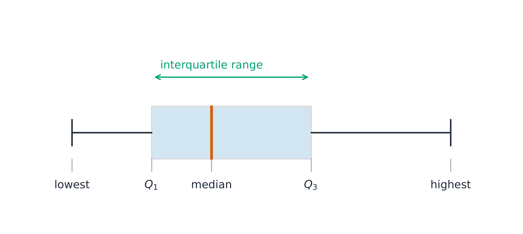
A boxplot 箱线图 draws the five-number summary: a box from $Q_1$ to $Q_3$ with the median inside, and whiskers to the most extreme non-outlier values. A point is an outlier if it lies more than $1.5\times\text{IQR}$ beyond a quartile – a rule you may be asked to apply. Boxplots are ideal for comparing several groups side by side.
Worked example. A dataset has $Q_1=20$ and $Q_3=32$, so $\text{IQR}=12$. The outlier fences are $Q_1-1.5(12)=2$ and $Q_3+1.5(12)=50$. Any value below $2$ or above $50$ is flagged as an outlier.
العربية
الرسم الصندوقي يرسم ملخص الخمس أرقام: صندوق من $Q_1$ إلى $Q_3$ مع الوسيط بداخله، وعيون للقيم المتطرفة الأكثر تطرفاً غير المتطرفة. النقطة تعتبر قيمة متطرفة إذا كانت تبعد أكثر من $1.5\times\text{IQR}$ عن أحد الربيعات – وهي قاعدة قد يُطلب منك تطبيقها. الرسم الصندوقي مثالي لمقارنة عدة مجموعات جنباً إلى جنب.
مثال محلل. مجموعة بيانات بها $Q_1=20$ و$Q_3=32$، إذن $\text{IQR}=12$. حدود القيم المتطرفة هي $Q_1-1.5(12)=2$ و$Q_3+1.5(12)=50$. أي قيمة أقل من $2$ أو أعلى من $50$ تُصنف كقيمة متطرفة.
رسم صندوقي يظهر الربيعات والمدىرسم صندوقي يرسم ملخص الخمس أرقام؛ الصندوق يغطي المدى الربيعي
Explore · استكشف
Explore the five-number summary as a boxplot · استكشف ملخص الخمس أرقام كمخطط صندوقي
Drag $Q_1$, the median, and $Q_3$ to see the box (its length is the IQR) and how the median's position inside the box reveals skew — a median close to $Q_1$ signals a right-skewed distribution. · اسحب $Q_1$، الوسيط، و$Q_3$ لرؤية الصندوق (طول هو IQR) وكيف يكشف موقع الوسيط داخل الصندوق عن الانحراف — الوسيط القريب من $Q_1$ يشير إلى توزيع منحرف لليمين.
Comparing Distributions of a Quantitative Variable · مقارنة توزيعات المتغير الكمي
Syllabus · المنهج
English
Enduring Understanding (UNC-1): Graphical representations and statistics allow us to identify and represent key features of data.
Learning Objective UNC-1.N: Compare graphical representations for multiple sets of quantitative data. [Skill 2.D]
UNC-1.N.1 Any of the graphical representations, e.g., histograms, side-by-side boxplots, etc., can be used to compare two or more independent samples on center, variability, clusters, gaps, outliers, and other features.
Learning Objective UNC-1.O: Compare summary statistics for multiple sets of quantitative data. [Skill 2.D]
UNC-1.O.1 Any of the numerical summaries (e.g., mean, standard deviation, relative frequency, etc.) can be used to compare two or more independent samples.
العربية
الفهم الدائم (UNC-1): تُمكّننا التمثيلات البيانية والإحصاءات من تحديد وميزة الملامح الرئيسية للبيانات.
هدف التعلم UNC-1.N: مقارنة التمثيلات البيانية لمجموعات متعددة من البيانات الكمية. [مهارة 2.D]
UNC-1.N.1 يمكن استخدام أي من التمثيلات البيانية، مثل المدرجات التكرارية، والرسومات الصندوقية جنباً إلى جنب، إلخ، لمقارنة عينتين مستقلتين أو أكثر من حيث المركز، والتشتت، والتكتلات، والفجوات، والقيم الشاذة، والميزات الأخرى.
هدف التعلم UNC-1.O: مقارنة الإحصاءات الموجزة لمجموعات متعددة من البيانات الكمية. [مهارة 2.D]
UNC-1.O.1 يمكن استخدام أي من الملخصات العددية (مثل المتوسط، والانحراف المعياري، والتردد النسبي، إلخ) لمقارنة عينتين مستقلتين أو أكثر.
Source: College Board AP Course and Exam Description · المصدر: وصف دورة وامتحان College Board AP
English
To compare two or more groups, compare shape, center, and spread, and mention outliers – always with comparative words ("Group A has a higher median than Group B") and in context. Do not just describe each group separately; make the comparison explicit.
العربية
لمقارنة مجموعتين أو أكثر، قارن الشكل والمركز والتشتت، واذكر القيم المتطرفة – دائماً بكلمات مقارنة ("المجموعة أ لها وسيط أعلى من المجموعة ب") وفي السياق. لا تصف كل مجموعة على حدة فقط؛ اجعل المقارنة صريحة.
Explore · استكشف
Compare distributions with box plots · قارن التوزيعات بمخططات الصناديق
A box plot draws the five-number summary. Placing two box plots on the same scale compares their centre (median), spread (IQR = box width) and skew at a glance — the fair way to compare groups. · المخطط الصندوقي يرسم ملخص الخمس أرقام. وضع مخططين صندوقيين على نفس المقياس يقارن مركزهما (الوسيط)، انتشارهما (IQR = عرض الصندوق) وانحرافهما بنظرة واحدة — الطريقة العادلة لمقارنة المجموعات.
1.10
The Normal Distribution · التوزيع الطبيعي
Syllabus · المنهج
Enduring Understanding
Learning Objective
Essential Knowledge
VAR-2
The normal distribution can be used to represent some population distributions.
VAR-2.A
Compare a data distribution to the normal distribution model. [Skill 2.D]
VAR-2.A.1 A parameter is a numerical summary of a population.
VAR-2.A.2 Some sets of data may be described as approximately normally distributed. A normal curve is mound-shaped and symmetric. The parameters of a normal distribution are the population mean, $\mu$, and the population standard deviation, $\sigma$.
VAR-2.A.3 For a normal distribution, approximately 68% of the observations are within 1 standard deviation of the mean, approximately 95% of observations are within 2 standard deviations of the mean, and approximately 99.7% of observations are within 3 standard deviations of the mean. This is called the empirical rule.
VAR-2.A.4 Many variables can be modeled by a normal distribution.
Illustrative examples for VAR-2.A:
Variables that can be modeled by a normal distribution:
Body temperature
Weight of a loaf of bread
VAR-2.B
Determine proportions and percentiles from a normal distribution. [Skill 3.A]
VAR-2.B.1 A standardized score for a particular data value is calculated as (data value − mean)/(standard deviation), and measures the number of standard deviations a data value falls above or below the mean.
VAR-2.B.2 One example of a standardized score is a $z$-score, which is calculated as $z\text{-score} = \left(\dfrac{x_i - \mu}{\sigma}\right)$. A $z$-score measures how many standard deviations a data value is from the mean.
VAR-2.B.3 Technology, such as a calculator, a standard normal table, or computer-generated output, can be used to find the proportion of data values located on a given interval of a normally distributed random variable.
VAR-2.B.4 Given the area of a region under the graph of the normal distribution curve, it is possible to use technology, such as a calculator, a standard normal table, or computer-generated output, to estimate parameters for some populations.
VAR-2.C
Compare measures of relative position in data sets. [Skill 2.D]
VAR-2.C.1 Percentiles and $z$-scores may be used to compare relative positions of points within a data set or between data sets.
Source: College Board AP Course and Exam Description · المصدر: وصف دورة وامتحان College Board AP
English
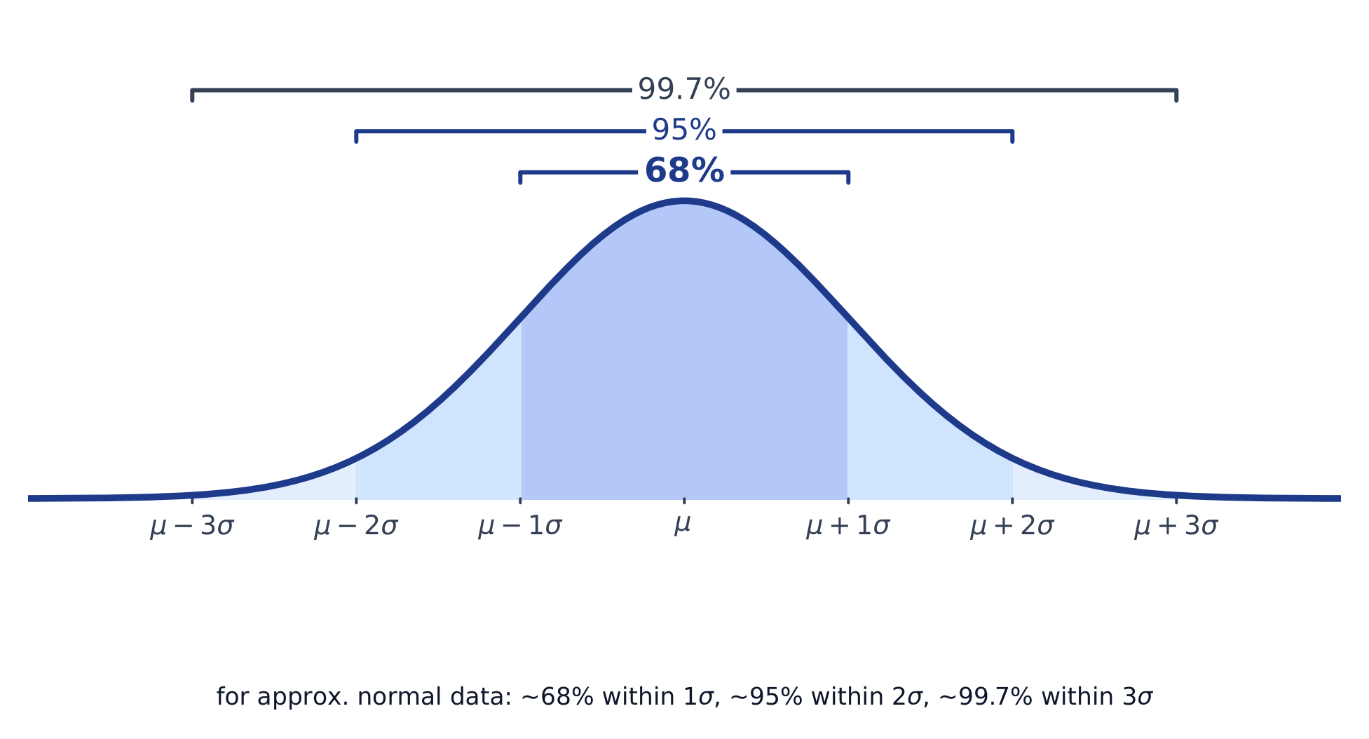
A normal distribution 正态分布 is a symmetric, bell-shaped model described by its mean $\mu$ and standard deviation $\sigma$. The empirical rule 经验法则 (68–95–99.7): about 68% of values lie within $1\sigma$ of the mean, 95% within $2\sigma$, and 99.7% within $3\sigma$.
A $z$-score 标准分数 measures how many standard deviations a value is from the mean:
$$z=\frac{x-\mu}{\sigma}.$$
Convert to a $z$-score, then use the normal table or technology to find the proportion (area) below, above, or between values – and reverse the process to find a value from a given percentile.
Worked example. Test scores are normal with $\mu=500$ and $\sigma=100$. A score of $700$ has $z=\dfrac{700-500}{100}=2$. By the empirical rule, $95\%$ of scores lie within $2\sigma$, so $2.5\%$ lie above $700$ – meaning a $700$ is at about the $97.5$th percentile.
العربية
التوزيع الطبيعي هو نموذج متماثل على شكل جرس توصف بمتوسطه $\mu$ وانحرافه المعياري $\sigma$. القاعدة التجريبية (68-95-99.7): حوالي 68% من القيم تقع ضمن $1\sigma$ من المتوسط، 95% ضمن $2\sigma$، و99.7% ضمن $3\sigma$.
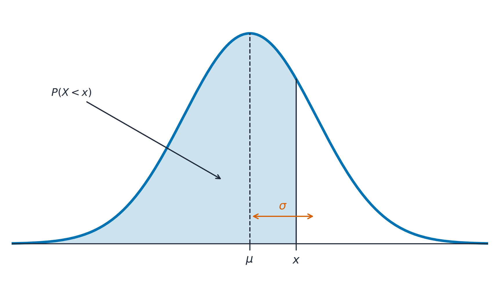
المنحنى الطبيعي: الاحتمال هو المساحة تحته، متمركز حول المتوسط الحسابي
الدرجة المعيارية$z$ تقيس كم انحراف معياري تبعد القيمة عن المتوسط:
$$z=\frac{x-\mu}{\sigma}.$$
حوّل إلى درجة معيارية $z$، ثم استخدم الجدول الطبيعي أو التكنولوجيا لإيجاد النسبة (المساحة) تحت، فوق، أو بين القيم – وعكس العملية لإيجاد قيمة من مستوى مئوي محدد.
مثال محلل. درجات الاختبار تتبع توزيعاً طبيعياً بمتوسط $\mu=500$ وانحراف معياري $\sigma=100$. الدرجة $700$ لها درجة معيارية $z=\dfrac{700-500}{100}=2$. بالقاعدة التجريبية، يقع $95\%$ من الدرجات ضمن $2\sigma$، لذا تقع $2.5\%$ فوق $700$ – مما يعني أن الدرجة $700$ تقبع عند المستوى المئوي تقريباً $97.5$.
المنحنى الطبيعي والقاعدة التجريبية 68-95-99.7
Explore · استكشف
Explore area under the normal curve · استكشف المساحة تحت المنحنى الطبيعي
The proportion of data below a value equals the area under the curve to its left. Shade a tail or a central band to see the 68–95–99.7 empirical rule and read a $z$-score as an area. · نسبة البيانات أقل من قيمة تساوي المساحة تحت المنحنى على يسارها. ظلل ذيلاً أو حزاماً مركزياً لرؤية قاعدة ⟦68–95–99.7⟧ التجريبية واقرأ درجة $z$ كمساحة.
Are Two Variables Related? · هل هناك علاقة بين متغيرين؟
Syllabus · المنهج
English
Enduring Understanding (VAR-1): Given that variation may be random or not, conclusions are uncertain.
Learning Objective VAR-1.D: Identify questions to be answered about possible relationships in data. [Skill 1.A]
VAR-1.D.1 Apparent patterns and associations in data may be random or not.
العربية
الفهم الدائم (VAR-1): بما أن التباين قد يكون عشوائياً أو غير ذلك، فإن الاستنتاجات تكون غير مؤكدة.
هدف التعلم VAR-1.D: تحديد الأسئلة التي يجب الإجابة عنها حول العلاقات المحتملة في البيانات. [مهارة 1.A]
VAR-1.D.1 قد تكون الأنماط والروابط الظاهرة في البيانات عشوائية أو غير ذلك.
Source: College Board AP Course and Exam Description · المصدر: وصف دورة وامتحان College Board AP
English
Two-variable data let us ask whether two characteristics are associated 关联 – whether knowing one tells you something about the other. An explanatory variable 解释变量 (the "input") may help predict a response variable 响应变量 (the "output"). Association is not the same as causation.
العربية
بيانات المتغيرين تسمح لنا بسؤال ما إذا كان خاصيتان مرتبطتان – هل معرفة واحدة تخبرنا بشيء عن الأخرى. المتغير التوضيحي (الـ "المدخل") قد يساعد في التنبؤ بـالمتغير الاستجابة (الـ "المخرج"). الارتباط ليس نفس السببية.
2.2
Two Categorical Variables · متغيران فئويان
Syllabus · المنهج
English
Enduring Understanding (UNC-1): Graphical representations and statistics allow us to identify and represent key features of data.
Learning Objective UNC-1.P: Compare numerical and graphical representations for two categorical variables. [Skill 2.D]
UNC-1.P.1 Side-by-side bar graphs, segmented bar graphs, and mosaic plots are examples of bar graphs for one categorical variable, broken down by categories of another categorical variable.
UNC-1.P.2 Graphical representations of two categorical variables can be used to compare distributions and/or determine if variables are associated.
UNC-1.P.3 A two-way table, also called a contingency table, is used to summarize two categorical variables. The entries in the cells can be frequency counts or relative frequencies.
UNC-1.P.4 A joint relative frequency is a cell frequency divided by the total for the entire table.
العربية
الفهم الدائم (UNC-1): تُمكّننا التمثيلات البيانية والإحصاءات من تحديد وميزة الملامح الرئيسية للبيانات.
هدف التعلم UNC-1.P: مقارنة التمثيلات العددية والبيانية لمتغيرين فئيين. [مهارة 2.D]
UNC-1.P.1 المدرجات الشريطية جنباً إلى جنب، والمدرجات الشريطية المجزأة، ومخططات الفسيفساء أمثلة على المدرجات الشريطية لمتغير فئ واحد، مقسمة حسب فئات متغير فئ آخر.
UNC-1.P.2 يمكن استخدام التمثيلات البيانية لمتغيرين فئيين لمقارنة التوزيعات و/أو تحديد ما إذا كانت المتغيرات مرتبطة.
UNC-1.P.3 جدول ثنائي الأبعاد، يُعرف أيضًا باسم جدول التباين، يُستخدم لتلخيص متغيرين فئويين. يمكن أن تكون المدخلات في الخلايا أعدادًا تكرارية أو تكرارات نسبية.
UNC-1.P.4 التكرار النسبي المشترك هو تكرار الخلية مقسومًا على الإجمالي الكلي للجدول بأكمله.
Source: College Board AP Course and Exam Description · المصدر: وصف دورة وامتحان College Board AP
English
A two-way table 双向表 (contingency table) counts individuals by two categorical variables at once. A marginal distribution 边缘分布 is a row or column total written as a fraction of the grand total (the totals themselves are just counts). Comparing the inside cells shows whether the variables are related.
العربية
جدول ثنائي الأبعاد (جدول ترابط) يعدّ الأفراد بناءً على متغيرين فئيين في آن واحد. التوزيع الهامشي هو مجموع صف أو عمود مكتوباً ككسر من المجموع الكلي (المجموعات نفسها مجرد أعداد). مقارنة الخلايا الداخلية تظهر ما إذا كان المتغيران مرتبطين.
2.3
Comparing Groups with Conditional Distributions · مقارنة المجموعات بالتوزيعات الشرطية
Syllabus · المنهج
English
Enduring Understanding (UNC-1): Graphical representations and statistics allow us to identify and represent key features of data.
Learning Objective UNC-1.Q: Calculate statistics for two categorical variables. [Skill 2.C]
UNC-1.Q.1 The marginal relative frequencies are the row and column totals in a two-way table divided by the total for the entire table.
UNC-1.Q.2 A conditional relative frequency is a relative frequency for a specific part of the contingency table (e.g., cell frequencies in a row divided by the total for that row).
Learning Objective UNC-1.R: Compare statistics for two categorical variables. [Skill 2.D]
UNC-1.R.1 Summary statistics for two categorical variables can be used to compare distributions and/or determine if variables are associated.
العربية
الفهم الدائم (UNC-1): تُمكّننا التمثيلات البيانية والإحصاءات من تحديد وميزة الملامح الرئيسية للبيانات.
هدف التعلم UNC-1.Q: حساب الإحصاءات لمتغيرين فئويين. [المهارة 2.C]
UNC-1.Q.1 التكرارات النسبية الهامشية هي مجاميع الصفوف والأعمدة في الجدول الثنائي الأبعاد مقسومة على الإجمالي الكلي للجدول بأكمله.
UNC-1.Q.2 التكرار النسبي الشرطي هو تكرار نسبي جزء محدد من جدول التباين (مثل تكرارات الخلايا في صف مقسومًا على إجمالي ذلك الصف).
هدف التعلم UNC-1.R: مقارنة الإحصاءات لمتغيرين فئويين. [المهارة 2.D]
UNC-1.R.1 يمكن استخدام الإحصاءات الوصفية لمتغيرين فئويين لمقارنة التوزيعات و/أو تحديد ما إذا كانت المتغيرات مرتبطة.
Source: College Board AP Course and Exam Description · المصدر: وصف دورة وامتحان College Board AP
English
A conditional distribution 条件分布 is the distribution of one variable within a fixed category of the other (found by dividing each cell by its row or column total). If the conditional distributions differ across groups, the two variables are associated; if they are the same, there is no association. Segmented bar charts 分段条形图 or mosaic plots display them.
العربية
التوزيع الشرطي هو توزيع أحد المتغيرات داخل فئة ثابتة من الآخر (يُوجد بقسمة كل خلية على مجموع صفها أو عمودها). إذا اختلفت التوزيعات الشرطية عبر المجموعات، فإن المتغيرين مرتبطان؛ إذا كانت متطابقة، فلا يوجد ارتباط. تعرض الرسوم البيانية الشريطية المجزأة أو مخططات الفسيفساء هذه التوزيعات.
2.4
Scatterplots for Two Quantitative Variables · مخطط التشتث للمتغيرين الكمي
Syllabus · المنهج
English
Enduring Understanding (UNC-1): Graphical representations and statistics allow us to identify and represent key features of data.
Learning Objective UNC-1.S: Represent bivariate quantitative data using scatterplots. [Skill 2.B]
UNC-1.S.1 A bivariate quantitative data set consists of observations of two different quantitative variables made on individuals in a sample or population.
UNC-1.S.2 A scatterplot shows two numeric values for each observation, one corresponding to the value on the $x$-axis and one corresponding to the value on the $y$-axis.
UNC-1.S.3 An explanatory variable is a variable whose values are used to explain or predict corresponding values for the response variable.
Enduring Understanding (DAT-1): Regression models may allow us to predict responses to changes in an explanatory variable.
Learning Objective DAT-1.A: Describe the characteristics of a scatter plot. [Skill 2.A]
DAT-1.A.1 A description of a scatter plot includes form, direction, strength, and unusual features.
DAT-1.A.2 The direction of the association shown in a scatterplot, if any, can be described as positive or negative.
DAT-1.A.3 A positive association means that as values of one variable increase, the values of the other variable tend to increase. A negative association means that as values of one variable increase, values of the other variable tend to decrease.
DAT-1.A.4 The form of the association shown in a scatterplot, if any, can be described as linear or non-linear to varying degrees.
DAT-1.A.5 The strength of the association is how closely the individual points follow a specific pattern, e.g., linear, and can be shown in a scatterplot. Strength can be described as strong, moderate, or weak.
DAT-1.A.6 Unusual features of a scatter plot include clusters of points or points with relatively large discrepancies between the value of the response variable and a predicted value for the response variable.
العربية
الفهم الدائم (UNC-1): تُمكّننا التمثيلات البيانية والإحصاءات من تحديد وميزة الملامح الرئيسية للبيانات.
هدف التعلم UNC-1.S: تمثيل البيانات الكمية ثنائية المتغيرات باستخدام المخططات الانتشارية. [المهارة 2.B]
UNC-1.S.1 تتكون مجموعة بيانات كمية ثنائية المتغيرات من ملاحظات لمتغيرين كميين مختلفين تم إجراؤها على أفراد في عينة أو مجتمع.
UNC-1.S.2 يعرض المخطط الانتشاري قيمتين عدديتين لكل ملاحظة، واحدة تقابل القيمة على محور $x$ والأخرى تقابل القيمة على محور $y$.
UNC-1.S.3 المتغير المفسر هو متغير تُستخدم قيمه لتفسير أو التنبؤ بالقيم المقابلة للمتغير الاستجابة.
فهم دائم (DAT-1): قد تسمح لنا نماذج الانحدار بالتنبؤ بالاستجابات للتغيرات في متغير مفسر.
هدف التعلم DAT-1.A: وصف خصائص المخطط الانتشاري. [المهارة 2.A]
DAT-1.A.1 يتضمن وصف المخطط الانتشاري الشكل والاتجاه والقوة والخصائص غير العادية.
DAT-1.A.2 يمكن وصف اتجاه الارتباط الموضح في المخطط الانتشاري، إن وجد، بأنه موجب أو سالب.
DAT-1.A.3 يعني الارتباط الموجب أنه كلما زادت قيم أحد المتغيرين، زادت قيم المتغير الآخر. ويعني الارتباط السالب أنه كلما زادت قيم أحد المتغيرين، انخفضت قيم المتغير الآخر.
DAT-1.A.4 يمكن وصف شكل الارتباط الموضح في المخطط الانتشاري، إن وجد، بأنه خطي أو غير خطي بدرجات متفاوتة.
DAT-1.A.5 قوة الارتباط هي مدى اقتراب النقاط الفردية من نمط معين، مثل الخطي، ويمكن عرضها في مخطط انتشاري. يمكن وصف القوة بأنها قوية أو معتدلة أو ضعيفة.
DAT-1.A.6 تشمل الخصائص غير العادية للمخطط الانتشاري تجمعات للنقاط أو نقاط ذات انحرافات كبيرة نسبيًا بين قيمة المتغير الاستجابة وقيمة متوقعة له.
Source: College Board AP Course and Exam Description · المصدر: وصف دورة وامتحان College Board AP
English
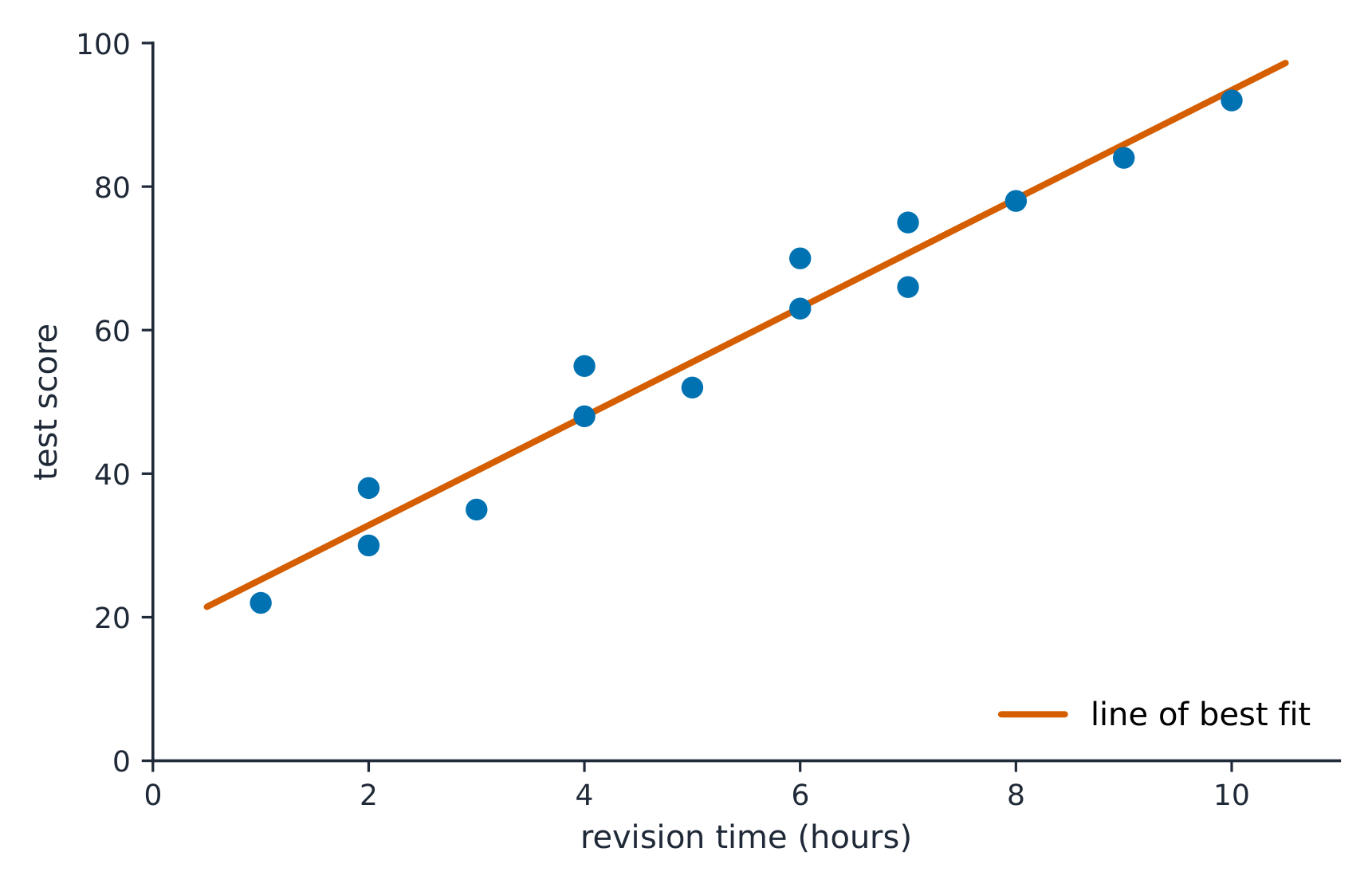
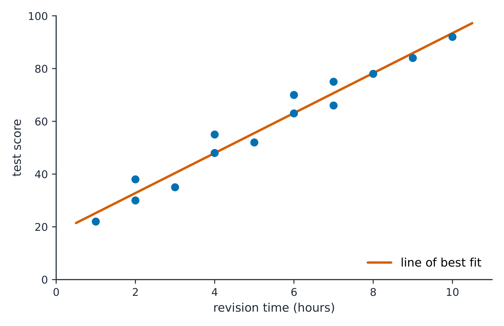
A scatterplot 散点图 plots each individual as a point, explanatory variable on the $x$-axis and response on the $y$-axis. Describe it with DUFS: Direction (positive/negative), Unusual features (outliers, clusters), Form (linear or curved), and Strength (how tightly the points follow the pattern) – always in context.
العربية
يُصوّر مخطط التشتت كل فرد كنقطة، مع وضع المتغير المفسر على محور $x$ والمتغير المستجيب على محور $y$. صغّره باستخدام DUFS: الاتجاه (إيجابي/سلبي)، الخصائص غير المعتادة (نقاط شاذة، تجمعات)، الشكل (خطي أو منحنى)، والقوة (مدى تقارب النقاط مع النمط) – دائماً في السياق.
خط أفضل انحدار يمر عبر وسط النقاط المتناثرة
2.5
Correlation · الارتباط
Syllabus · المنهج
English
Enduring Understanding (DAT-1): Regression models may allow us to predict responses to changes in an explanatory variable.
Learning Objective DAT-1.B: Determine the correlation for a linear relationship. [Skill 2.C]
DAT-1.B.1 The correlation, $r$, gives the direction and quantifies the strength of the linear association between two quantitative variables.
DAT-1.B.2 The correlation coefficient can be calculated by: $r = \dfrac{1}{n-1} \sum \left( \dfrac{x_i - \bar{x}}{s_x} \right) \left( \dfrac{y_i - \bar{y}}{s_y} \right)$. However, the most common way to determine $r$ is by using technology.
DAT-1.B.3 A correlation coefficient close to 1 or $-1$ does not necessarily mean that a linear model is appropriate.
Learning Objective DAT-1.C: Interpret the correlation for a linear relationship. [Skill 4.B]
DAT-1.C.1 The correlation, $r$, is unit-free, and always between $-1$ and 1, inclusive. A value of $r = 0$ indicates that there is no linear association. A value of $r = 1$ or $r = -1$ indicates that there is a perfect linear association.
DAT-1.C.2 A perceived or real relationship between two variables does not mean that changes in one variable cause changes in the other. That is, correlation does not necessarily imply causation.
العربية
فهم دائم (DAT-1): قد تسمح لنا نماذج الانحدار بالتنبؤ بالاستجابات للتغيرات في متغير مفسر.
هدف التعلم DAT-1.B: تحديد معامل الارتباط لعلاقة خطية. [المهارة 2.C]
DAT-1.B.1 يعطي معامل الارتباط، $r$، الاتجاه ويقيس قوة الارتباط الخطي بين متغيرين كميين.
DAT-1.B.2 يمكن حساب معامل الارتباط بواسطة: $r = \dfrac{1}{n-1} \sum \left( \dfrac{x_i - \bar{x}}{s_x} \right) \left( \dfrac{y_i - \bar{y}}{s_y} \right)$. ومع ذلك، فإن الطريقة الأكثر شيوعًا لتحديد $r$ هي باستخدام التكنولوجيا.
DAT-1.B.3 لا يعني بالضرورة أن نموذجًا خطيًا مناسبًا أن يكون معامل ارتباط قريبًا من 1 أو $-1$.
هدف التعلم DAT-1.C: تفسير معامل الارتباط لعلاقة خطية. [المهارة 4.B]
DAT-1.C.1 معامل الارتباط $r$ لا وحدة له، ويقع دائمًا بين $-1$ و1 بشكل شامل. تشير القيمة $r = 0$ إلى عدم وجود ارتباط خطي. تشير القيم $r = 1$ أو $r = -1$ إلى وجود ارتباط خطي مثالي.
DAT-1.C.2 لا يعني وجود علاقة مدركة أو حقيقية بين متغيرين أن التغيرات في أحدهما تسبب تغيرات في الآخر. أي أن الارتباط لا يعني بالضرورة السببية.
Source: College Board AP Course and Exam Description · المصدر: وصف دورة وامتحان College Board AP
English
What r actually measures
The correlation coefficient 相关系数$r$ measures the strength and direction of a linear relationship. It runs from $-1$ to $1$: near $\pm 1$ is strong linear, near $0$ is weak linear. $r$ has no units and does not change if you swap the variables. Warnings: $r$ only measures linear strength, it is not resistant to outliers, and a strong $r$ does not prove causation.
العربية
ماذا يقيسه r فعلياً
يقيس معامل الارتباط$r$قوة واتجاه العلاقة الخطية. ويتراوح بين $-1$ و$1$: ما يقترب من $\pm 1$ يشير إلى علاقة خطية قوية، وما يقترب من $0$ يشير إلى علاقة خطية ضعيفة. لا يمتلك $r$وحدات قياس ولا يتغير إذا قمت بتبديل المتغيرات. تحذيرات: يقيس $r$قوة خطية فقط، وهو غير مقاوم للنقاط الشاذة، ولا تثبت $r$ القوية السببية.
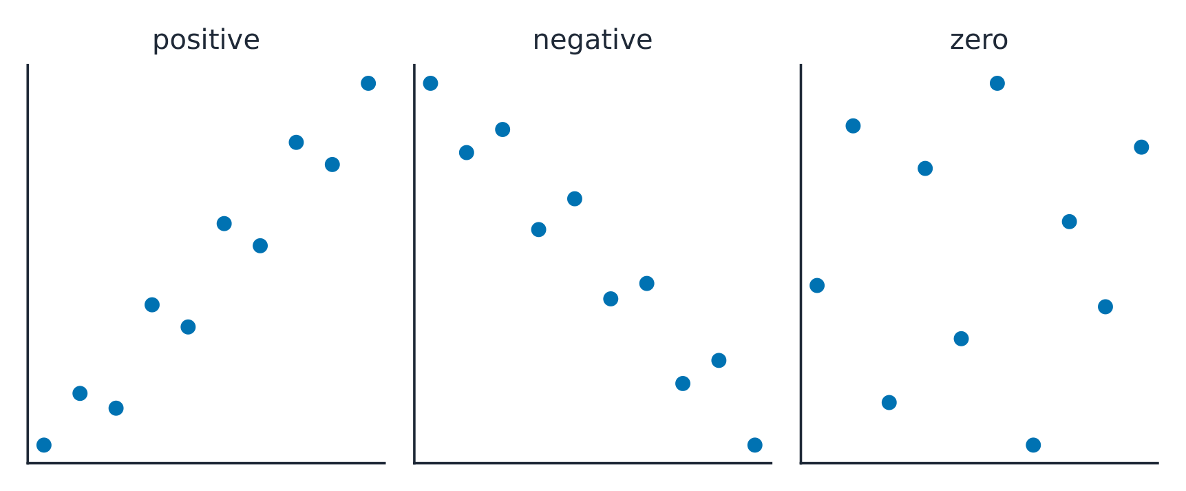
الارتباط الإيجابي يرتفع معاً؛ الانحدار السلبي يتحرك في اتجاهات معاكسة
Explore · استكشف
Strength of a linear relationship · قوة العلاقة الخطية
Correlation$r$ runs from $-1$ to $1$: near $\pm1$ the points hug a line, near 0 they scatter. Change it and watch the cloud tighten or spread. · الارتباط$r$ يتراوح بين $-1$ و$1$: بالقرب من $\pm1$ تتجمع النقاط حول خط، قرب 0 تتناثر. غيّره وشاهد السحابة تتكثف أو تنتشر.
2.6
Linear Regression Models · نماذج الانحدار الخطي
Syllabus · المنهج
English
Enduring Understanding (DAT-1): Regression models may allow us to predict responses to changes in an explanatory variable.
Learning Objective DAT-1.D: Calculate a predicted response value using a linear regression model. [Skill 2.C]
DAT-1.D.1 A simple linear regression model is an equation that uses an explanatory variable, $x$, to predict the response variable, $y$.
DAT-1.D.2 The predicted response value, denoted by $\hat{y}$, is calculated as $\hat{y} = a + bx$, where $a$ is the $y$-intercept and $b$ is the slope of the regression line, and $x$ is the value of the explanatory variable.
DAT-1.D.3 Extrapolation is predicting a response value using a value for the explanatory variable that is beyond the interval of $x$-values used to determine the regression line. The predicted value is less reliable as an estimate the further we extrapolate.
العربية
فهم دائم (DAT-1): قد تسمح لنا نماذج الانحدار بالتنبؤ بالاستجابات للتغيرات في متغير مفسر.
هدف التعلم DAT-1.D: حساب قيمة استجابة متوقعة باستخدام نموذج انحدار خطي. [المهارة 2.C]
DAT-1.D.1 نموذج الانحدار الخطي البسيط هو معادلة تستخدم متغيرًا مفسرًا، $x$، للتنبؤ بالمتغير الاستجابة، $y$.
DAT-1.D.2 يتم حساب قيمة الاستجابة المتوقعة، المشار إليها بـ $\hat{y}$، بالمعادلة $\hat{y} = a + bx$، حيث $a$ هو التقاطع على المحور $y$ و$b$ هو ميل خط الانحدار، و$x$ هي قيمة المتغير المفسر.
DAT-1.D.3 الاستنباط الخارجي هو التنبؤ بقيمة استجابة باستخدام قيمة للمتغير المفسر تقع خارج نطاق قيم $x$ المستخدمة لتحديد خط الانحدار. تقل موثوقية القيمة المتوقعة كتقدير كلما ابتعدنا أكثر في الاستنباط الخارجي.
Source: College Board AP Course and Exam Description · المصدر: وصف دورة وامتحان College Board AP
English
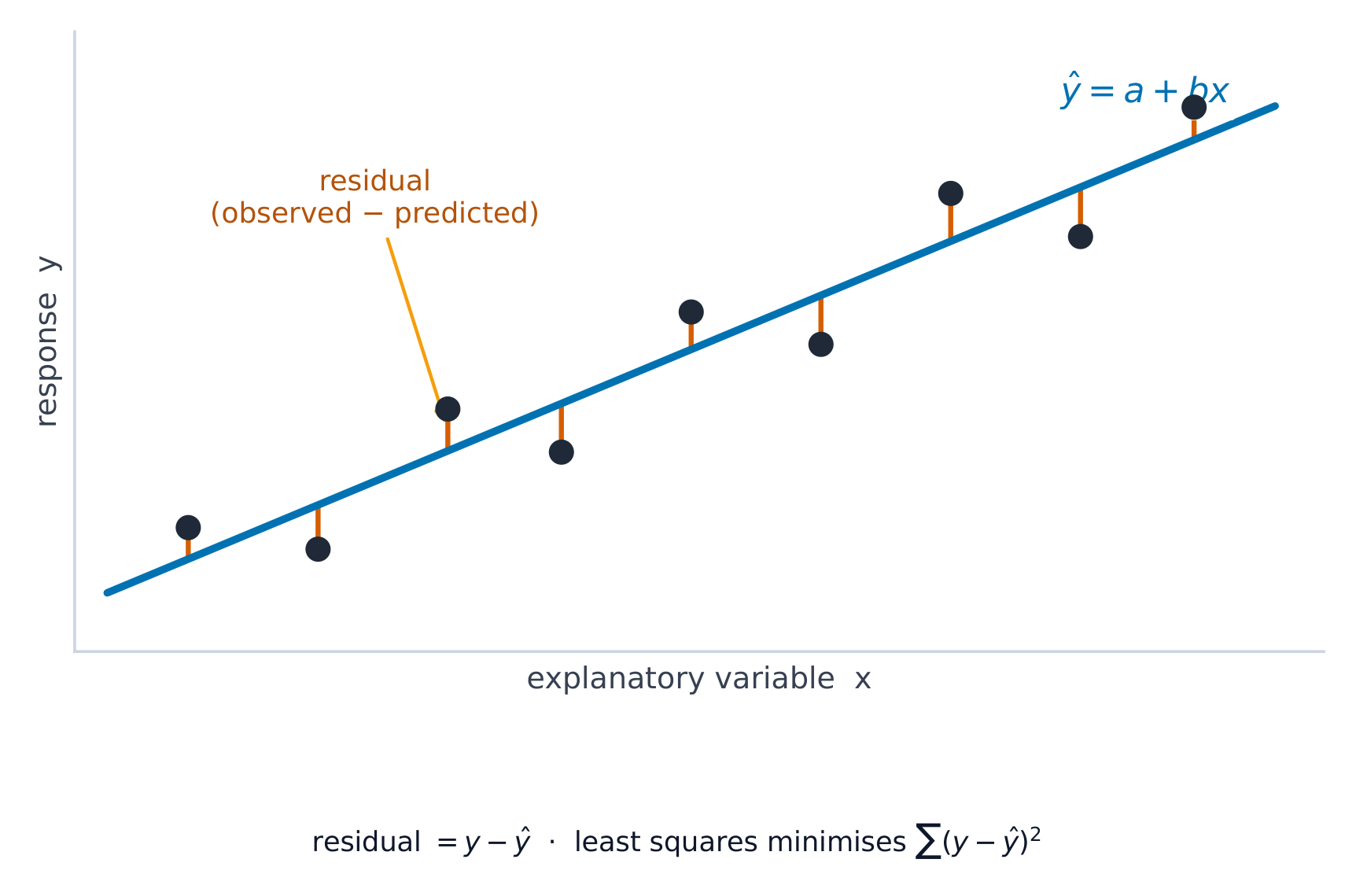
The least-squares regression line 最小二乘回归线 predicts the response: $\hat{y}=a+bx$, where $\hat{y}$ is the predicted response. The slope 斜率$b$ is the predicted change in $y$ per one-unit increase in $x$; the $y$-intercept 截距$a$ is the predicted $y$ when $x=0$. Interpret both in context and with units – a graded skill. Avoid extrapolation 外推 (predicting far outside the data).
Worked example. A study of hours studied ($x$) and test score ($y$) gives $\hat{y}=20+3x$. The slope means each extra hour of study is associated with a predicted $3$-point increase. A student who studies $5$ hours is predicted to score $\hat{y}=20+3(5)=35$.
العربية
يتنبأ خط الانحدار بأقل مربعات بالاستجابة: $\hat{y}=a+bx$، حيث $\hat{y}$ هي الاستجابة المتوقعة. يمثل الميل$b$ التغير المتوقع في $y$ لكل زيادة مقدارها وحدة واحدة في $x$؛ بينما يمثل المقطع الصادي$y$$a$ القيمة المتوقعة لـ $y$ عندما $x=0$. فسر كليهما في السياق ومع الوحدات – مهارة متدرجة. تجنب التشعب (التنبؤ بعيداً عن نطاق البيانات).
مثال محلول. دراسة حول ساعات الدراسة ($x$) والنتيجة في الاختبار ($y$) أعطت $\hat{y}=20+3x$. يعني الميل أن كل ساعة دراسة إضافية ترتبط بزيادة متوقعة بمقدار $3$ نقطة. يُتوقع لطالب يدرس $5$ ساعات أن يحقق نتيجة قدرها $\hat{y}=20+3(5)=35$.
Explore · استكشف
Fit a least-squares line · ضبط خط أقل مربعات
A regression line is the best straight-line fit, minimising the squared vertical distances. Its slope predicts how $y$ changes per unit of $x$. · خط الانحدار هو أفضل ضبط خط مستقيم، يقلل المربعات الرأسية. ميله يتنبأ بكيفية تغير $y$ لكل وحدة من $x$.
2.7
Residuals · البواقي
Syllabus · المنهج
English
Enduring Understanding (DAT-1): Regression models may allow us to predict responses to changes in an explanatory variable.
Learning Objective DAT-1.E: Represent differences between measured and predicted responses using residual plots. [Skill 2.B]
DAT-1.E.1 The residual is the difference between the actual value and the predicted value: $\text{residual} = y - \hat{y}$.
DAT-1.E.2 A residual plot is a plot of residuals versus explanatory variable values or predicted response values.
Learning Objective DAT-1.F: Describe the form of association of bivariate data using residual plots. [Skill 2.A]
DAT-1.F.1 Apparent randomness in a residual plot for a linear model is evidence of a linear form to the association between the variables.
DAT-1.F.2 Residual plots can be used to investigate the appropriateness of a selected model.
العربية
فهم دائم (DAT-1): قد تسمح لنا نماذج الانحدار بالتنبؤ بالاستجابات للتغيرات في متغير مفسر.
هدف التعلم DAT-1.E: تمثيل الفروقات بين الاستجابات المقاسة والمتوقعة باستخدام مخططات البواقي. [المهارة 2.B]
DAT-1.E.1 الباقي هو الفرق بين القيمة الفعلية والقيمة المتوقعة: $\text{residual} = y - \hat{y}$.
DAT-1.E.2 مخطط البواقي هو رسم بياني للبواقي مقابل قيم المتغير المفسر أو قيم الاستجابة المتوقعة.
هدف التعلم DAT-1.F: وصف شكل ارتباط البيانات ثنائية المتغيرات باستخدام مخططات البواقي. [المهارة 2.A]
DAT-1.F.1 العشوائية الظاهرة في مخطط البواقي لنموذج خطي هي دليل على شكل خطي للارتباط بين المتغيرات.
DAT-1.F.2 يمكن استخدام مخططات البواقي للتحقق من مدى مناسبة النموذج المختار.
Source: College Board AP Course and Exam Description · المصدر: وصف دورة وامتحان College Board AP
English
Least-squares regression
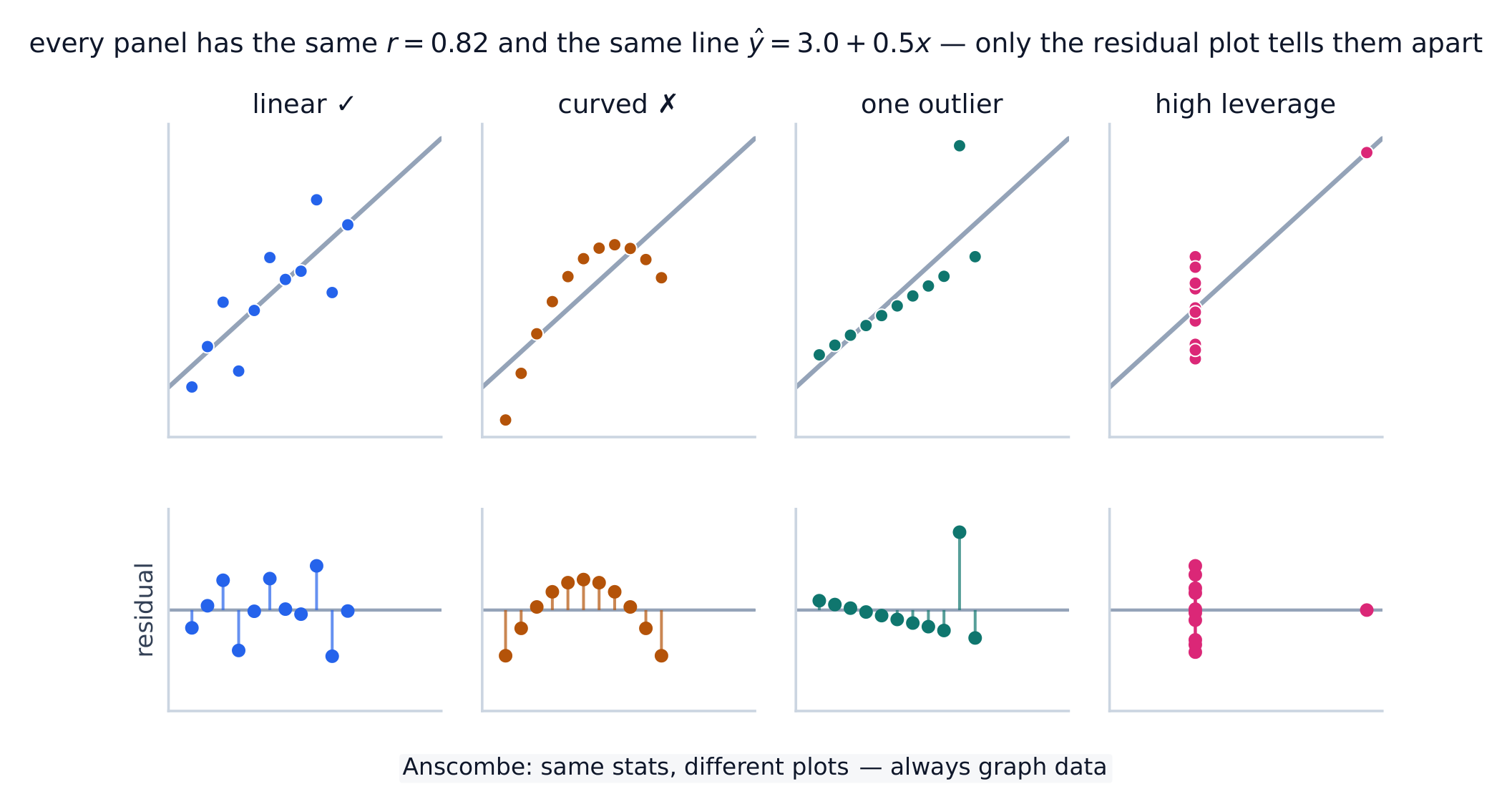
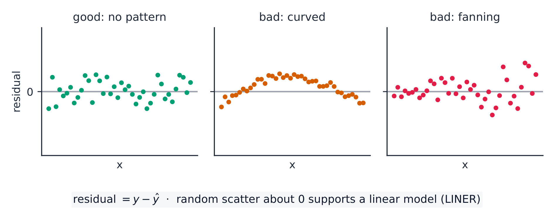
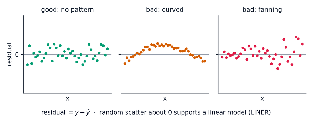
A residual 残差 is actual minus predicted, $y-\hat{y}$: how far a point sits above (+) or below (−) the line. A residual plot 残差图 graphs residuals against $x$. If it shows no pattern (random scatter), a linear model is appropriate; a curved or fanning pattern means the linear model is a poor fit.
Worked example. Continuing the study above, a student who studied $5$ hours actually scored $40$. The residual is $y-\hat{y}=40-35=+5$: the line under-predicted by $5$ points, so this point sits above the line.
العربية
انحدار المربعات الصغرى
الباقي هو الفعلي مطروحاً منه المتوقع، $y-\hat{y}$: المسافة التي تبعد بها النقطة فوق (+) أو تحت (−) الخط. يرسم مخطط البواقي البواقي مقابل $x$. إذا أظهر لا نمطاً (تشتت عشوائي)، فإن النموذج الخطي مناسب؛ أما النمط المنحني أو المتسع فيعني أن النموذج الخطي غير ملائم جيداً.
مثال محلول. استكمالاً للدراسة أعلاه، طالب درس $5$ ساعات حققت فعلياً نتيجة $40$. الباقي هو $y-\hat{y}=40-35=+5$: مما يعني أن الخط تنبأ بشكل أقل بمقدار $5$ نقاط، لذا تقع هذه النقطة فوق الخط.
تحذير بخصوص $r$ والخط: جميع مجموعات البيانات الأربع لها نفس $r=0.82$ ونفس $\hat{y}=3.0+0.5x$، لكن الأولى فقط هي خطية حقاً. مخططات التشتت متشابهة تقريباً — إلا أن مخطط البواقي أسفل كل منها يكشف عن المنحنى والنقطة الشاذة والنقطة ذات التأثير العالي.
2.8
Least-Squares Regression and Its Fit · الانحدار بأقل مربعات وملاءمته
Syllabus · المنهج
English
Enduring Understanding (DAT-1): Regression models may allow us to predict responses to changes in an explanatory variable.
Learning Objective DAT-1.G: Estimate parameters for the least-squares regression line model. [Skill 2.C]
DAT-1.G.1 The least-squares regression model minimizes the sum of the squares of the residuals and contains the point $(\bar{x}, \bar{y})$.
DAT-1.G.2 The slope, $b$, of the regression line can be calculated as $b = r \left( \dfrac{s_y}{s_x} \right)$ where $r$ is the correlation between $x$ and $y$, $s_y$ is the sample standard deviation of the response variable, $y$, and $s_x$ is the sample standard deviation of the explanatory variable, $x$.
DAT-1.G.3 Sometimes, the $y$-intercept of the line does not have a logical interpretation in context.
DAT-1.G.4 In simple linear regression, $r^2$ is the square of the correlation, $r$. It is also called the coefficient of determination. $r^2$ is the proportion of variation in the response variable that is explained by the explanatory variable in the model.
Learning Objective DAT-1.H: Interpret coefficients for the least-squares regression line model. [Skill 4.B]
DAT-1.H.1 The coefficients of the least-squares regression model are the estimated slope and $y$-intercept.
DAT-1.H.2 The slope is the amount that the predicted $y$-value changes for every unit increase in $x$.
DAT-1.H.3 The $y$-intercept value is the predicted value of the response variable when the explanatory variable is equal to $0$. The formula for the $y$-intercept, $a$, is $a = \bar{y} - b\bar{x}$.
العربية
فهم دائم (DAT-1): قد تسمح لنا نماذج الانحدار بالتنبؤ بالاستجابات للتغيرات في متغير مفسر.
هدف التعلم DAT-1.G: تقدير معاملات نموذج خط الانحدار المربعات الصغرى. [مهارة 2.C]
DAT-1.G.1 يقلل نموذج الانحدار المربعات الصغرى مجموع مربعات البواقي ويحتوي على النقطة $(\bar{x}, \bar{y})$.
DAT-1.G.2 يمكن حساب ميل خط الانحدار، $b$، باستخدام $b = r \left( \dfrac{s_y}{s_x} \right)$ حيث $r$ هو معامل الارتباط بين $x$ و$y$، $s_y$ هو الانحراف المعياري للعينة للمتغير المستجيب، $y$، و$s_x$ هو الانحراف المعياري للعينة للمتغير التوضيحي، $x$.
DAT-1.G.3 أحيانًا، لا يكون للقاطع المحوري $y$ تفسير منطقي في السياق.
DAT-1.G.4 في الانحدار الخطي البسيط، $r^2$ هو مربع معامل الارتباط، $r$. يُسمى أيضًا معامل التحديد. $r^2$ يمثل نسبة التباين في المتغير المستجيب التي يفسرها المتغير التوضيحي في النموذج.
هدف التعلم DAT-1.H: تفسير المعاملات لنموذج خط الانحدار المربعات الصغرى. [مهارة 4.B]
DAT-1.H.1 معاملات نموذج الانحدار المربعات الصغرى هي الميل المقدر والقاطع المحوري $y$.
DAT-1.H.2 الميل هو مقدار التغير في القيمة المتوقعة لـ $y$ لكل زيادة بمقدار وحدة واحدة في $x$.
DAT-1.H.3 قيمة القاطع المحوري $y$ هي القيمة المتوقعة للمتغير المستجيب عندما يكون المتغير التوضيحي مساويًا لـ $0$. صيغة القاطع المحوري $y$، $a$، هي $a = \bar{y} - b\bar{x}$.
Source: College Board AP Course and Exam Description · المصدر: وصف دورة وامتحان College Board AP
English
The line minimizes the sum of squared residuals. Its fit is measured by:
$s$, the standard deviation of the residuals – the typical prediction error, in the response's units.
$r^2$, the coefficient of determination 决定系数 – the proportion of the variation in $y$ that the linear model explains (a value between $0$ and $1$; multiply by $100$ to state it as a percent). Report it in context: "$r^2 = 0.81$ means 81% of the variation in $y$ is explained by the linear relationship with $x$."
العربية
خط أقل المربعات يقلل مجموع المربعات للبقايا
يقلل الخط مجموع المربعات للبقايا. تُقاس ملاءمته بما يلي:
$r^2$، معامل التحديد – نسبة التباين في $y$ التي يفسرها النموذج الخطي (قيمة بين $0$ و$1$؛ اضرب في $100$ للتعبير عنها كنسبة مئوية). أدرجها في السياق: "يعني $r^2 = 0.81$ أن 81% من التباين في $y$ يُفسر بالعلاقة الخطية مع $x$."
coefficient of determination/ˌkəʊɪˈfɪʃənt ɒv dɪˌtɜːmɪˈneɪʃn/
معامل التحديد
high-leverage/haɪ ˈliːvərɪdʒ/
ذو التأثير العالي (High-leverage)
influential/ˌɪnfluːˈenʃl/
مؤثر
2.9
Departures from Linearity · الانحرافات عن الخطية
Syllabus · المنهج
English
Enduring Understanding (DAT-1): Regression models may allow us to predict responses to changes in an explanatory variable.
Learning Objective DAT-1.I: Identify influential points in regression. [Skill 2.A]
DAT-1.I.1 An outlier in regression is a point that does not follow the general trend shown in the rest of the data and has a large residual when the Least Squares Regression Line (LSRL) is calculated.
DAT-1.I.2 A high-leverage point in regression has a substantially larger or smaller $x$-value than the other observations have.
DAT-1.I.3 An influential point in regression is any point that, if removed, changes the relationship substantially. Examples include much different slope, $y$-intercept, and/or correlation. Outliers and high leverage points are often influential.
Learning Objective DAT-1.J: Calculate a predicted response using a least-squares regression line for a transformed data set. [Skill 2.C]
DAT-1.J.1 Transformations of variables, such as evaluating the natural logarithm of each value of the response variable or squaring each value of the explanatory variable, can be used to create transformed data sets, which may be more linear in form than the untransformed data.
DAT-1.J.2 Increased randomness in residual plots after transformation of data and/or movement of $r^2$ to a value closer to 1 offers evidence that the least-squares regression line for the transformed data is a more appropriate model to use to predict responses to the explanatory variable than the regression line for the untransformed data.
العربية
فهم دائم (DAT-1): قد تسمح لنا نماذج الانحدار بالتنبؤ بالاستجابات للتغيرات في متغير مفسر.
هدف التعلم DAT-1.I: تحديد النقاط المؤثرة في الانحدار. [مهارة 2.A]
DAT-1.I.1 القيمة الشاذة في الانحدار هي نقطة لا تتبع الاتجاه العام الموضح في بقية البيانات ولها باقٍ كبير عند حساب خط الانحدار المربعات الصغرى (LSRL).
DAT-1.I.2 النقطة ذات التأثير العالي في الانحدار لها قيمة $x$ أكبر أو أصغر بشكل ملحوظ مقارنة بالقيم التي تمتلكها المشاهدات الأخرى.
DAT-1.I.3 النقطة المؤثرة في الانحدار هي أي نقطة إذا تم إزالتها تتغير العلاقة بشكل كبير. تشمل الأمثلة اختلافًا كبيرًا في الميل، والقاطع المحوري $y$، و/أو معامل الارتباط. غالبًا ما تكون القيم الشاذة والنقاط ذات التأثير العالي مؤثرة.
هدف التعلم DAT-1.J: حساب استجابة متوقعة باستخدام خط انحدار المربعات الصغرى لمجموعة بيانات محولة. [مهارة 2.C]
DAT-1.J.1 يمكن استخدام تحويلات المتغيرات، مثل حساب اللوغاريتم الطبيعي لكل قيمة للمتغير المستجيب أو تربيع كل قيمة للمتغير التوضيحي، لإنشاء مجموعات بيانات محولة قد تكون أكثر خطيًا من البيانات الأصلية.
DAT-1.J.2 زيادة العشوائية في مخططات البقايا بعد تحويل البيانات و/أو تحرك $r^2$ إلى قيمة أقرب إلى 1 يقدم دليلاً على أن خط الانحدار المربعات الصغرى للبيانات المحولة هو نموذج أكثر ملاءمة للاستخدام للتنبؤ بالاستجابات للمتغير التوضيحي مقارنة بخط الانحدار للبيانات الأصلية.
Source: College Board AP Course and Exam Description · المصدر: وصف دورة وامتحان College Board AP
English
Some points strongly affect the line. A high-leverage 高杠杆 point has an extreme $x$-value; an influential 有影响的 point noticeably changes the slope or $r$ when removed; an outlier here is a point with a large residual. When the pattern is curved, transform a variable (e.g. take a log) to straighten it, then fit a line to the transformed data.
العربية
بعض النقاط تؤثر بشدة على الخط. النقطة ذات التأثير العالي لها قيمة extreme على $x$-axis؛ النقطة المؤثرة تغير الميل أو $r$ بشكل ملحوظ عند إزالتها؛ أما النقطة الشاذة هنا فهي نقطة ذات باقي كبير. عندما يكون النمط منحنيًا، قم بـ تحويل متغير (مثل أخذ اللوغاريتم) لتقويمه، ثم-fit خط على البيانات المحولة.
2.9
Exam tips · نصائح للامتحان
English
On a scatterplot describe direction, form, strength, and outliers; $r$ ranges $-1$ to $1$.
Correlation is not causation — a lurking variable can drive both.
Interpret the slope of the least-squares line in context ("per one unit of $x$, predicted $y$ changes by $b$").
Check a residual plot: no pattern means a line fits; a curve means it does not. Avoid extrapolation.
$r^2$ is the fraction of variation in $y$ explained by the model.
العربية
على مخطط التشتت صف الاتجاه والشكل والقوة والنقاط الشاذة؛ تتراوح $r$ بين $-1$ و$1$.
الارتباط ليس سببية – قد يكون هناك متغير خفي يقود كلاهما.
فسر ميل خط أقل المربعات في السياق ("لكل وحدة واحدة من $x$، يتغير $y$ المتوقع بمقدار $b$").
تحقق من مخطط البواقي: عدم وجود نمط يعني أن الخط مناسب؛ المنحنى يعني أنه غير مناسب. تجنب التشعب.
Can We Trust the Data We Collected? · هل يمكننا الوثوق بالبيانات التي جمعناها؟
Syllabus · المنهج
English
Enduring Understanding (VAR-1): Given that variation may be random or not, conclusions are uncertain.
Learning Objective VAR-1.E: Identify questions to be answered about data collection methods. [Skill 1.A]
VAR-1.E.1 Methods for data collection that do not rely on chance result in untrustworthy conclusions.
العربية
الفهم الدائم (VAR-1): بما أن التباين قد يكون عشوائياً أو غير ذلك، فإن الاستنتاجات تكون غير مؤكدة.
هدف التعلم VAR-1.E: تحديد الأسئلة المراد الإجابة عنها حول طرق جمع البيانات. [مهارة 1.A]
VAR-1.E.1 تؤدي طرق جمع البيانات التي لا تعتمد على الحظ إلى استنتاجات غير موثوقة.
Source: College Board AP Course and Exam Description · المصدر: وصف دورة وامتحان College Board AP
English
A conclusion is only as good as the data behind it. How data are collected decides what you may conclude – whether you can generalize to a population 总体, and whether you can claim cause and effect. Poorly collected data can be worse than none.
العربية
المستخلص بقدر جودة البيانات التي يستند إليها. كيفية جمع البيانات تحدد ما يمكنك استنتاجه – سواء كان بإمكانك تعميم النتائج على مجتمع إحصائي، أو ادعاء السببية والتأثير. البيانات السيئة قد تكون أسوأ من عدم وجود بيانات.
3.2
Observational Studies and Experiments · الدراسات الرصدية والتجارب
Syllabus · المنهج
English
Enduring Understanding (DAT-2): The way we collect data influences what we can and cannot say about a population.
Learning Objective DAT-2.A: Identify the type of a study. [Skill 1.C]
DAT-2.A.1 A population consists of all items or subjects of interest.
DAT-2.A.2 A sample selected for study is a subset of the population.
DAT-2.A.3 In an observational study, treatments are not imposed. Investigators examine data for a sample of individuals (retrospective) or follow a sample of individuals into the future collecting data (prospective) in order to investigate a topic of interest about the population. A sample survey is a type of observational study that collects data from a sample in an attempt to learn about the population from which the sample was taken.
DAT-2.A.4 In an experiment, different conditions (treatments) are assigned to experimental units (participants or subjects).
Learning Objective DAT-2.B: Identify appropriate generalizations and determinations based on observational studies. [Skill 4.A]
DAT-2.B.1 It is only appropriate to make generalizations about a population based on samples that are randomly selected or otherwise representative of that population.
DAT-2.B.2 A sample is only generalizable to the population from which the sample was selected.
DAT-2.B.3 It is not possible to determine causal relationships between variables using data collected in an observational study.
العربية
فهم دائم (DAT-2): طريقة جمعنا للبيانات تؤثر على ما يمكننا وما لا يمكننا قوله عن مجتمع.
هدف التعلم DAT-2.A: تحديد نوع الدراسة. [مهارة 1.C]
DAT-2.A.1 المجتمع يتكون من جميع العناصر أو الموضوعات محل الاهتمام.
DAT-2.A.2 العينة المختارة للدراسة هي جزء فرعي من المجتمع.
DAT-2.A.3 في الدراسة الرصدية، لا يتم فرض معالجات. يفحص الباحثون البيانات لعينة من الأفراد (دراسة استرجاعية) أو يتبعون عينة من الأفراد مستقبلاً لجمع البيانات (دراسة مستقبلية) للتحقيق في موضوع معين يتعلق بالمجتمع. المسح العيني هو نوع من الدراسات الرصدية يجمع البيانات من عينة بهدف التعرف على المجتمع الذي أُخذت منه العينة.
DAT-2.A.4 في التجربة، تُخصص ظروف مختلفة (معالجات) لوحدات التجريبية (المشاركين أو الموضوعين).
هدف التعلم DAT-2.B: تحديد تعميمات وتعيينات مناسبة بناءً على الدراسات الرصدية. [مهارة 4.A]
DAT-2.B.1 من المناسب فقط إجراء تعميمات حول مجتمع ما بناءً على عينات تم اختيارها عشوائياً أو أنها ممثلة لهذا المجتمع بطرق أخرى.
DAT-2.B.2 يمكن تعميم العينة فقط على المجتمع الذي تم اختيار العينة منه.
DAT-2.B.3 لا يمكن تحديد العلاقات السببية بين المتغيرات باستخدام البيانات المجمعة في دراسة رصدية.
Source: College Board AP Course and Exam Description · المصدر: وصف دورة وامتحان College Board AP
English
In an observational study 观察性研究 you measure individuals without trying to influence them. It can show association, but not causation, because lurking variables may explain the link.
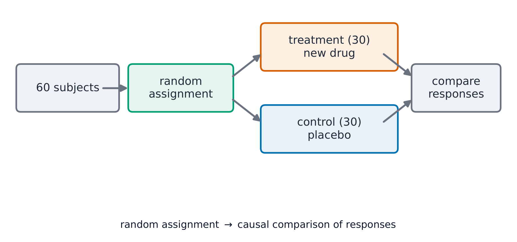
In an experiment 实验 you deliberately impose a treatment 处理 and compare responses. A well-designed experiment can establish cause and effect.
العربية
في الدراسة الرصدية تقيس الأفراد دون محاولة التأثير عليهم. يمكن أن تظهر الارتباط، لكنها لا تثبت السببية، لأن المتغيرات الخفية قد تفسر الرابط.
Observational study or experiment? · دراسة رصدية أم تجربة؟
In an experiment the researcher imposes a treatment (and can show cause); an observational study only records what already happens (and can show association, not cause). · في التجربة يقوم الباحث بـفرض معالجة (ويمكن إثبات السبب)؛ أما الدراسة الرصدية فتكتفي بتسجيل ما يحدث بالفعل (ويمكن إظهار الارتباط، لا السبب).
3.3
Random Sampling · العين العشوائية
Syllabus · المنهج
English
Enduring Understanding (DAT-2): The way we collect data influences what we can and cannot say about a population.
Learning Objective DAT-2.C: Identify a sampling method, given a description of a study. [Skill 1.C]
DAT-2.C.1 When an item from a population can be selected only once, this is called sampling without replacement. When an item from the population can be selected more than once, this is called sampling with replacement.
DAT-2.C.2 A simple random sample (SRS) is a sample in which every group of a given size has an equal chance of being chosen. This method is the basis for many types of sampling mechanisms. A few examples of mechanisms used to obtain SRSs include numbering individuals and using a random number generator to select which ones to include in the sample, ignoring repeats, using a table of random numbers, or drawing a card from a deck without replacement.
DAT-2.C.3 A stratified random sample involves the division of a population into separate groups, called strata, based on shared attributes or characteristics (homogeneous grouping). Within each stratum a simple random sample is selected, and the selected units are combined to form the sample.
DAT-2.C.4 A cluster sample involves the division of a population into smaller groups, called clusters. Ideally, there is heterogeneity within each cluster, and clusters are similar to one another in their composition. A simple random sample of clusters is selected from the population to form the sample of clusters. Data are collected from all observations in the selected clusters.
DAT-2.C.5 A systematic random sample is a method in which sample members from a population are selected according to a random starting point and a fixed, periodic interval.
DAT-2.C.6 A census selects all items/subjects in a population.
Learning Objective DAT-2.D: Explain why a particular sampling method is or is not appropriate for a given situation. [Skill 1.C]
DAT-2.D.1 There are advantages and disadvantages for each sampling method depending upon the question that is to be answered and the population from which the sample will be drawn.
العربية
فهم دائم (DAT-2): طريقة جمعنا للبيانات تؤثر على ما يمكننا وما لا يمكننا قوله عن مجتمع.
هدف التعلم DAT-2.C: تحديد طريقة取样، بناءً على وصف الدراسة. [مهارة 1.C]
DAT-2.C.1 عندما يمكن اختيار عنصر واحد من المجتمع مرة واحدة فقط، يسمى هذا Sampling without replacement. عندما يمكن اختيار عنصر من المجتمع أكثر من مرة، يسمى هذا Sampling with replacement.
DAT-2.C.2 العينة العشوائية البسيطة (SRS) هي عينة يكون فيها لكل مجموعة بحجم معين فرصة متساوية للاختيار. هذه الطريقة هي الأساس للعديد من أنواع آليات取样. بعض أمثلة الآليات المستخدمة للحصول على SRSs تشمل ترقيم الأفراد واستخدام مولد الأرقام العشوائية لتحديد أيهم يجب تضمينهم في العينة، وتجاهل التكرارات،或使用随机数表,或从一副牌中抽取一张卡而不放回。
DAT-2.C.3 العينة العشوائية الطبقيّة تتضمن تقسيم المجتمع إلى مجموعات منفصلة تسمى طبقات، بناءً على سمات أو خصائص مشتركة (تجميع متجانس). داخل كل طبقة يتم اختيار عينة عشوائية بسيطة، وتُجمع الوحدات المختارة لتكوين العينة.
DAT-2.C.4 العينة العنقوديّة تتضمن تقسيم المجتمع إلى مجموعات أصغر تسمى عنقوديات. من المثالي أن يكون هناك تباين داخلي في كل عنقودية، وأن تكون العنقوديات متشابهة فيما بينها في تكوينها. يتم اختيار عينة عشوائية بسيطة من العنقوديات من المجتمع لتكوين عينة العنقوديات. يتم جمع البيانات من جميع الملاحظات في العنقوديات المختارة.
DAT-2.C.5 العينة العشوائية المنتظمة هي طريقة يتم فيها اختيار أفراد العينة من المجتمع وفقاً لنقطة بداية عشوائية وفاصل زمني ثابت ومتكرر.
DAT-2.C.6 التعداد العام يختار جميع العناصر/المواضيع في المجتمع.
الهدف التعليمي DAT-2.D: اشرح لماذا تكون طريقة عينات معينة مناسبة أو غير مناسبة لموقف محدد. [مهارة 1.C]
DAT-2.D.1 لكل طريقة عينات مزايا وعيوب اعتماداً على السؤال المراد الإجابة عليه والمجتمع الذي سيتم سحب العينة منه.
Source: College Board AP Course and Exam Description · المصدر: وصف دورة وامتحان College Board AP
English
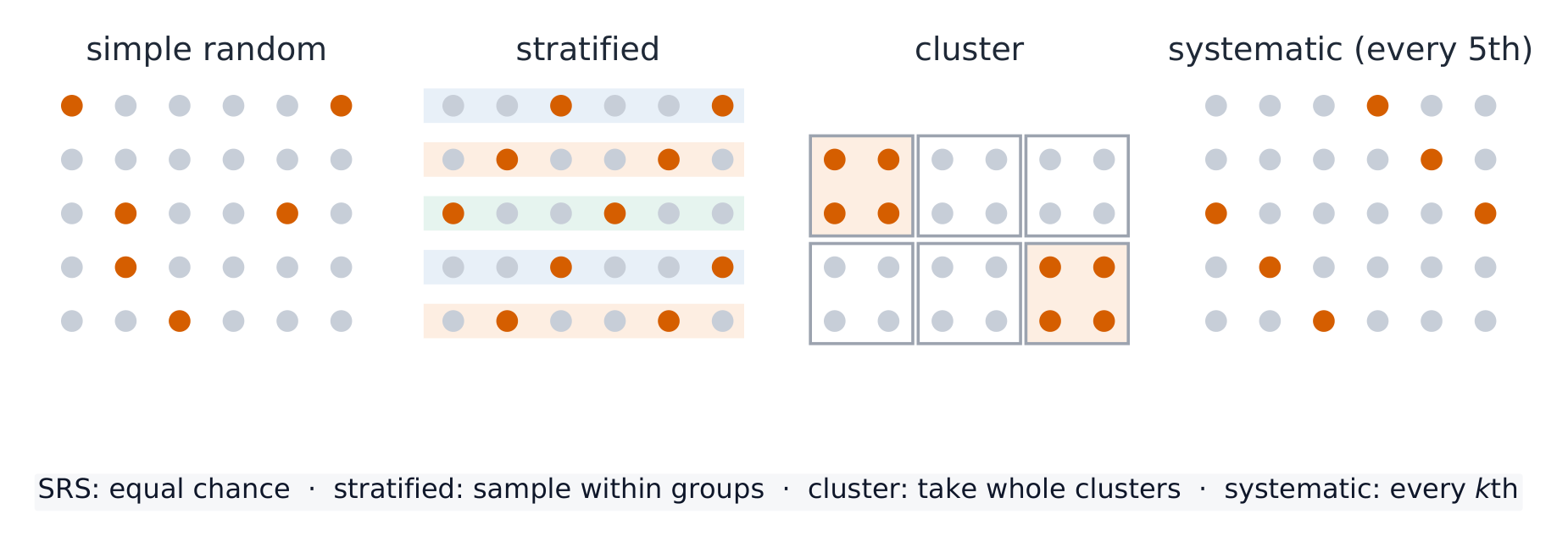
To learn about a population you take a sample 样本. Random sampling 随机抽样 protects against selection bias 偏差 and lets you generalize (it cannot fix undercoverage, nonresponse, or response bias — see below). Common designs:
Simple random sample (SRS) 简单随机样本: every group of the chosen size is equally likely.
Stratified 分层: split the population into similar strata, then sample within each.
Cluster 整群: split into clusters, randomly choose whole clusters.
Systematic 系统: pick every $k$th individual from a random start.
A convenience sample 方便样本 or voluntary response sample is not random and is biased.
Worked example. To survey a school, an administrator lists all students by grade and randomly selects $20$ from each grade. This is a stratified sample – the grades are the strata – which guarantees every grade is represented, unlike an SRS that might by chance draw few from one grade.
العربية
لمعرفة مجتمع إحصائي تأخذ عينة. العينة العشوائية تحمي من التحيز في الاختيار وتسمح بالتعميم (لا يمكنها إصلاح التغطية الناقصة أو عدم الاستجابة أو تحيز الاستجابة – انظر أدناه). التصاميم الشائعة:
العينة العشوائية البسيطة (SRS): كل مجموعة بحجم الاختيار محتملة بالتساوي.
طبقات: تقسيم المجتمع إلى طبقات متشابهة، ثم أخذ عينات داخل كل طبقة.
عنقود: التقسيم إلى عناقيد، واختيار عناقيد كاملة عشوائياً.
منهجية: اختيار كل $k$ فرد بدءاً من نقطة عشوائية.
أربعة تصاميم للعينة العشوائية: من يتم اختياره، وكيف
العينة المريحة أو عينة الاستجابة الطوعيةليست عشوائية ومحيّزة.
مثال محلول. لاستطلاع رأي في مدرسة، يقوم مسؤول بإدراج جميع الطلاب حسب الصفوف ثم يختار $20$ عشوائياً من كل صف. هذه عينة مقسّمة طبقاتاً – حيث تمثل الصفوف الطبقات – مما يضمن تمثيل كل صف على الأقل، بعكس العينة العشوائية البسيطة التي قد تسحب عدداً قليلاً عن طريق الخطأ من أحد الصفوف.
نتائج عشوائية: النرد يجعل كل وجه متساوي الاحتمال تحت ظروف عادلة
3.4
When Sampling Goes Wrong · عندما تفشل العينة
Syllabus · المنهج
English
Enduring Understanding (DAT-2): The way we collect data influences what we can and cannot say about a population.
Learning Objective DAT-2.E: Identify potential sources of bias in sampling methods. [Skill 1.C]
DAT-2.E.1 Bias occurs when certain responses are systematically favored over others.
DAT-2.E.2 When a sample is comprised entirely of volunteers or people who choose to participate, the sample will typically not be representative of the population (voluntary response bias).
DAT-2.E.3 When part of the population has a reduced chance of being included in the sample, the sample will typically not be representative of the population (undercoverage bias).
DAT-2.E.4 Individuals chosen for the sample for whom data cannot be obtained (or who refuse to respond) may differ from those for whom data can be obtained (nonresponse bias).
DAT-2.E.5 Problems in the data gathering instrument or process result in response bias. Examples include questions that are confusing or leading (question wording bias) and self-reported responses.
DAT-2.E.6 Non-random sampling methods (for example, samples chosen by convenience or voluntary response) introduce potential for bias because they do not use chance to select the individuals.
العربية
فهم دائم (DAT-2): طريقة جمعنا للبيانات تؤثر على ما يمكننا وما لا يمكننا قوله عن مجتمع.
الهدف التعليمي DAT-2.E: حدد المصادر المحتملة للتحيز في طرق العينات. [مهارة 1.C]
DAT-2.E.1 يحدث التحيز عندما يتم تفضيل استجابات معينة بشكل منهجي على أخرى.
DAT-2.E.2 عندما تتكون العينة بالكامل من المتطوعين أو الأشخاص الذين اختاروا المشاركة، عادةً ما لا تكون العينة ممثلة للمجتمع (تحيز الاستجابة الطوعية).
DAT-2.E.3 عندما يكون لدى جزء من المجتمع فرصة منخفضة للإدراج في العينة، عادةً ما لا تكون العينة ممثلة للمجتمع (تحيز التغطية الناقصة).
DAT-2.E.4 الأفراد المختارين للعينة الذين لا يمكن الحصول على بياناتهم (أو الذين يرفضون الاستجابة) قد يختلفون عن أولئك الذين يمكن الحصول على بياناتهم (تحيز عدم الاستجابة).
DAT-2.E.5 تؤدي المشاكل في أداة أو عملية جمع البيانات إلى تحيز الاستجابة. تشمل الأمثلة الأسئلة المربكة أو الموجهة (تحيز صياغة السؤال) والاستجابات ذاتية الإبلاغ.
DAT-2.E.6 طرق العينات غير العشوائية (على سبيل المثال، العينات المختارة بالراحة أو الاستجابة الطوعية) تُدخل احتمالية للتحيز لأنها لا تستخدم الحظ لاختيار الأفراد.
Source: College Board AP Course and Exam Description · المصدر: وصف دورة وامتحان College Board AP
English
Bias makes estimates systematically miss the truth:
Undercoverage 覆盖不足: some groups are left out of the sampling frame.
Nonresponse 无回应: selected people do not answer.
Response bias 回应偏差: people answer inaccurately (bad wording, sensitive topics).
Bias is about a consistent error in one direction – increasing the sample size does not fix it.
العربية
التحيز يجعل التقديرات تبتعد بشكل منهجي عن الحقيقة:
عدم التغطية الكافية: تُستبعد بعض المجموعات من إطار العينة.
عدم الاستجابة: الأشخاص المختارون لا يجيبون.
تحيز الاستجابة: يجيب الناس بشكل غير دقيق (صياغة سيئة، مواضيع حساسة).
التحيز يتعلق بخطأ ثابت في اتجاه واحد – زيادة حجم العينة لا يحل المشكلة.
العينات المريحة تفوت المجتمع: يتسلل التحيز عند عدم كون الاختيار عشوائياً
Enduring Understanding (VAR-3): Well-designed experiments can establish evidence of causal relationships.
Learning Objective VAR-3.A: Identify the components of an experiment. [Skill 1.C]
VAR-3.A.1 The experimental units are the individuals (which may be people or other objects of study) that are assigned treatments. When experimental units consist of people, they are sometimes referred to as participants or subjects.
VAR-3.A.2 An explanatory variable (or factor) in an experiment is a variable whose levels are manipulated intentionally. The levels or combination of levels of the explanatory variable(s) are called treatments.
VAR-3.A.3 A response variable in an experiment is an outcome from the experimental units that is measured after the treatments have been administered.
VAR-3.A.4 A confounding variable in an experiment is a variable that is related to the explanatory variable and influences the response variable and may create a false perception of association between the two.
Learning Objective VAR-3.B: Describe elements of a well-designed experiment. [Skill 1.B]
VAR-3.B.1 A well-designed experiment should include the following:
a. Comparisons of at least two treatment groups, one of which could be a control group.
b. Random assignment/allocation of treatments to experimental units.
c. Replication (more than one experimental unit in each treatment group).
d. Control of potential confounding variables where appropriate.
Learning Objective VAR-3.C: Compare experimental designs and methods. [Skill 1.C]
VAR-3.C.1 In a completely randomized design, treatments are assigned to experimental units completely at random. Random assignment tends to balance the effects of uncontrolled (confounding) variables so that differences in responses can be attributed to the treatments.
VAR-3.C.2 Methods for randomly assigning treatments to experimental units in a completely randomized design include using a random number generator, a table of random values, drawing chips without replacement, etc.
VAR-3.C.3 In a single-blind experiment, subjects do not know which treatment they are receiving, but members of the research team do, or vice versa.
VAR-3.C.4 In a double-blind experiment neither the subjects nor the members of the research team who interact with them know which treatment a subject is receiving.
VAR-3.C.5 A control group is a collection of experimental units either not given a treatment of interest or given a treatment with an inactive substance (placebo) in order to determine if the treatment of interest has an effect.
VAR-3.C.6 The placebo effect occurs when experimental units have a response to a placebo.
VAR-3.C.7 For randomized complete block designs, treatments are assigned completely at random within each block.
VAR-3.C.8 Blocking ensures that at the beginning of the experiment the units within each block are similar to each other with respect to at least one blocking variable. A randomized block design helps to separate natural variability from differences due to the blocking variable.
VAR-3.C.9 A matched pairs design is a special case of a randomized block design. Using a blocking variable, subjects (whether they are people or not) are arranged in pairs matched on relevant factors. Matched pairs may be formed naturally or by the experimenter. Every pair receives both treatments by randomly assigning one treatment to one member of the pair and subsequently assigning the remaining treatment to the second member of the pair. Alternately, each subject may get both treatments.
العربية
الفهم الدائم (VAR-3): التجارب المصممة جيداً يمكنها إثبات أدلة على العلاقات السببية.
الهدف التعليمي VAR-3.A: حدد مكونات التجربة. [مهارة 1.C]
VAR-3.A.1 وحدات التجربة هم الأفراد (والذين قد يكونون أشخاصاً أو أجساماً أخرى قيد الدراسة) الذين يتم تعيينهم للتلقي المعالجات. عندما تتكون وحدات التجربة من أشخاص، يُشار إليها أحياناً بالمشاركين أو الموضوعات.
VAR-3.A.2 المتغير التوضيحي (أو العامل) في التجربة هو متغير مستوياته يتم التلاعب بها عمداً. تُسمى مستويات المتغير(ات) التوضيحية أو مجموعاتها بالمعالجات.
VAR-3.A.3 المتغير الاستجابة في التجربة هو نتيجة من وحدات التجربة يتم قياسها بعد تطبيق المعالجات.
VAR-3.A.4 المتغير المخلّ في التجربة هو متغير مرتبط بالمتغير التوضيحي ويؤثر على متغير الاستجابة وقد يخلق إدراكاً خاطئاً للارتباط بين الاثنين.
الهدف التعليمي VAR-3.B: صف عناصر التجربة المصممة جيداً. [مهارة 1.B]
VAR-3.B.1 يجب أن تتضمن التجربة المصممة جيداً ما يلي:
أ. مقارنة مجموعتين معالجتين على الأقل، إحداهما قد تكون مجموعة تحكم.
ج. التكرار (أكثر من وحدة تجريبية واحدة في كل مجموعة معالجة).
د. التحكم في المتغيرات المخللة المحتملة حيثما كان ذلك مناسباً.
الهدف التعليمي VAR-3.C: قارن تصاميم التجارب وطرقها. [مهارة 1.C]
VAR-3.C.1 في التصميم العشوائي الكامل، يتم تخصيص المعالجات لوحدة التجربة تماماً عشوائياً. يميل التوزيع العشوائي إلى موازنة تأثيرات المتغيرات غير الخاضعة للتحكم (المخللة) بحيث يمكن نسب الفروقات في الاستجابات إلى المعالجات.
VAR-3.C.2 تشمل الطرق لتخصيص المعالجات عشوائياً لوحدة التجربة في التصميم العشوائي الكامل استخدام مولد الأرقام العشوائية، وجدول القيم العشوائية، وسحب الرقائق بدون إرجاع، إلخ.
VAR-3.C.3 في التجربة العمياء الواحدة، لا يعرف المشاركين أي معالجة يتلقونها، لكن أعضاء فريق البحث يفعلون، أو العكس صحيح.
VAR-3.C.4 في التجربة العمياء المزدوجة، لا يعرف المشاركون ولا أعضاء فريق البحث الذين يتفاعلون معهم أي معالجة يتلقها المشارك.
VAR-3.C.5 مجموعة التحكم هي مجموعة من وحدات التجربة إما غير مُعطاة معالجة مثيرة للاهتمام أو مُعطاة معالجة بمادة غير نشطة (دواء وهمي) لتحديد ما إذا كانت المعالجة المثيرة للاهتمام لها تأثير.
VAR-3.C.6 يحدث تأثير الدواء الوهمي عندما يكون لدى وحدات التجربة استجابة للدواء الوهمي.
VAR-3.C.7 بالنسبة لتصاميم الكتل العشوائية الكاملة، يتم تخصيص المعالجات تماماً عشوائياً داخل كل كتلة.
VAR-3.C.8 الضبط يضمن أنه في بداية التجربة تكون الوحدات داخل كل كتلة متشابهة فيما بينها فيما يتعلق بمتغير ضبط واحد على الأقل. يساعد التصميم العشوائي للكتل على فصل التباين الطبيعي عن الفروقات الناتجة عن متغير الضبط.
VAR-3.C.9 تصميم الأزواج المتطابقة هو حالة خاصة من تصميم الكتل العشوائية. باستخدام متغير تكتيل، يتم ترتيب الوحدات (سواء كانت أشخاصًا أو غيرهم) في أزواج متطابقة بناءً على عوامل ذات صلة. يمكن تكوين الأزواج المتطابقة بشكل طبيعي أو بواسطة الباحث. كل زوج يتلقى كلا المعاملتين عن طريق تعيين عشوائي معاملة واحدة لأحد أفراد الزوج ثم تعيين المعاملة المتبقية للفرع الثاني من الزوج. وبديلًا لذلك، قد تحصل كل وحدة على كلا المعاملتين.
Source: College Board AP Course and Exam Description · المصدر: وصف دورة وامتحان College Board AP
English
Good experiments follow three principles:
Comparison with a control group 对照组 (often a placebo 安慰剂).
Random assignment 随机分配 of subjects to treatments, to balance out other variables.
Replication 重复: enough subjects per treatment to see a real effect.
Confounding 混杂 occurs when another variable is tied to the treatment so their effects cannot be separated; random assignment guards against it. Blinding 盲法 hides who is getting which treatment to prevent expectation effects: in a single-blind 单盲 study only one side is kept unaware (usually the subjects, or only the people assessing the result), while in a double-blind 双盲 study neither the subjects nor the researchers who interact with them know, blocking both the placebo effect and biased assessment. Blocking 区组 groups similar subjects and randomizes within each block to reduce variability.
العربية
تتبع التجارب الجيدة ثلاث مبادئ:
المقارنة مع مجموعة تحكم (غالباً دواء وهمي).
التعيين العشوائي للموضوعات إلى المعالجات، لتوازن المتغيرات الأخرى.
التكرار: عدد كافٍ من الموضوعات لكل معالجة لرؤية تأثير حقيقي.
تجربة عشوائية تماماً تقارن بين مجموعة معالجة ومجموعة تحكم
يحدث التداخل عندما يرتبط متغير آخر بالمعالجة بحيث لا يمكن فصل تأثيراتها؛ protects التعيين العشوائي من ذلك. الإخفاء يخفي من يحصل على أي معالجة لمنع تأثيرات التوقع: في دراسة مفردة الإخفاء، طرف واحد فقط يُبقي مجهولاً (عادةً المشاركين، أو فقط الأشخاص الذين يقيسون النتيجة)، بينما في دراسة مزدوجة الإخفاءلا يعرف participants ولا الباحثون الذين يتفاعلون معهم، مما يحجب كل من تأثير الدواء الوهمي والتقييم المحيّز. الحجب يجمع موضوعات مشابهة ويوزع عشوائياً داخل كل حجب لتقليل التباين.
تجربة سريرية: يعزل التعيين العشوائي المعالجة عن التحكم
Choosing the Right Design · اختيار التصميم المناسب
Syllabus · المنهج
English
Enduring Understanding (VAR-3): Well-designed experiments can establish evidence of causal relationships.
Learning Objective VAR-3.D: Explain why a particular experimental design is appropriate. [Skill 1.C]
VAR-3.D.1 There are advantages and disadvantages for each experimental design depending on the question of interest, the resources available, and the nature of the experimental units.
العربية
الفهم الدائم (VAR-3): التجارب المصممة جيداً يمكنها إثبات أدلة على العلاقات السببية.
هدف التعلم VAR-3.D: اشرح لماذا يكون تصميم تجريبي معين مناسبًا. [مهارة 1.C]
VAR-3.D.1 لكل تصميم تجريبي مزايا وعيوب تعتمد على السؤال المعني، والموارد المتاحة، وطبيعة الوحدات التجريبية.
Source: College Board AP Course and Exam Description · المصدر: وصف دورة وامتحان College Board AP
English
Match the design to the goal: use a completely randomized design for uniform subjects; a randomized block design when a known variable (sex, age) affects the response; a matched-pairs design when each subject can serve as its own control. State how you would carry out the randomization.
العربية
طابق التصميم بالهدف: استخدم تصميماً عشوائياً تماماً لمواضيع موحدة؛ تصميماً عشوائياً محجوباً عندما يؤثر متغير معروف (مثل الجنس، العمر) على الاستجابة؛ تصميم الأزواج المتطابقة عندما يمكن لكل موضوع أن يكون سيطرة بنفسه. وضح كيفية إجراء التوزيع العشوائي.
3.7
What an Experiment Lets You Conclude · ما تسمح به التجربة استنتاجه
Syllabus · المنهج
English
Enduring Understanding (VAR-3): Well-designed experiments can establish evidence of causal relationships.
Learning Objective VAR-3.E: Interpret the results of a well-designed experiment. [Skill 4.B]
VAR-3.E.1 Statistical inference attributes conclusions based on data to the distribution from which the data were collected.
VAR-3.E.2 Random assignment of treatments to experimental units allows researchers to conclude that some observed changes are so large as to be unlikely to have occurred by chance. Such changes are said to be statistically significant.
VAR-3.E.3 Statistically significant differences between or among experimental treatment groups are evidence that the treatments caused the effect.
VAR-3.E.4 If the experimental units used in an experiment are representative of some larger group of units, the results of an experiment can be generalized to the larger group. Random selection of experimental units gives a better chance that the units will be representative.
العربية
الفهم الدائم (VAR-3): التجارب المصممة جيداً يمكنها إثبات أدلة على العلاقات السببية.
هدف التعلم VAR-3.E: فسّر نتائج تجربة مصممة جيدًا. [مهارة 4.B]
VAR-3.E.1 يُنسب الاستدلال الإحصائي النتائج المستندة إلى البيانات إلى التوزيع الذي جُمعت منه هذه البيانات.
VAR-3.E.2 يسمح التعيين العشوائي للمعاملات للوحدات التجريبية للباحثين بالاستنتاج بأن بعض التغيرات الملاحظة كبيرة جدًا بحيث يكون من غير المحتمل حدوثها بالصدفة. وتُسمى مثل هذه التغيرات ذات دلالة إحصائية.
VAR-3.E.3 الفروقات ذات الدلالة الإحصائية بين مجموعات معاملات تجريبية مختلفة هي دليل على أن المعاملات تسببت في التأثير.
VAR-3.E.4 إذا كانت الوحدات التجريبية المستخدمة في تجربة ما ممثلة لمجموعة أكبر منها، يمكن تعميم نتائج التجربة على المجموعة الأكبر. يعطي الاختيار العشوائي للوحدات التجريبية فرصة أفضل لأن تكون ممثلة.
Source: College Board AP Course and Exam Description · المصدر: وصف دورة وامتحان College Board AP
English
Two questions decide the scope of a conclusion:
Random assignment used? Then a significant difference can be attributed to the treatment (causation) – for these subjects.
Random sampling from a population? Then results generalize to that population.
Only an experiment with random assignment supports a cause-and-effect claim; only random sampling supports generalization. Say exactly which you have.
Worked example. Researchers randomly assign $100$volunteers to a new drug or a placebo, and the drug group improves significantly more. Because of the random assignment, the improvement can be attributed to the drug (causation) – but because the subjects were not randomly sampled, the conclusion applies only to these volunteers and does not automatically generalize to everyone.
العربية
سؤالان يحددان نطاق الاستنتاج:
هل تم استخدام التعيين العشوائي؟ إذاً يمكن نسب فرق كبير إلى المعالجة (السببية) – بالنسبة لهؤلاء المشاركين.
هل تم العينة العشوائية من مجتمع؟ إذاً تنطبق النتائج على ذلك المجتمع.
فقط تجربة بالتعيين العشوائي تدعم ادعاء السبب والنتيجة؛ فقط العينة العشوائية تدعم التعميم. قُل بالضبط ما لديك.
مثال محلول. قام الباحثون بتعيين $100$متطوعين عشوائياً لعلاج جديد أو دواء وهمي، وتحسنت مجموعة العلاج بشكل ملحوظ أكثر. بسبب التعيين العشوائي، يمكن انتساب التحسن إلى العلاج (السببية) – ولكن بما أن المشاركين لم يتم اختيارهم عشوائياً، فإن الاستنتاج ينطبق فقط على هؤلاء المتطوعين ولا يتعمم تلقائياً للجميع.
3.7
Exam tips · نصائح للامتحان
English
Distinguish an observational study (finds association) from an experiment (can show causation).
Good sampling is random (SRS, stratified, cluster) — beware bias (voluntary response, undercoverage, nonresponse).
Good experiments use control, randomization, and replication; blocking handles a known nuisance variable.
Only a randomized experiment supports a cause-and-effect conclusion.
Name the population, sample, and any confounding clearly.
العربية
ميّز بين الدراسة الرصدية (تجد ارتباطاً) والتجربة (يمكنها إظهار السببية).
العينة الجيدة عشوائية (SRS، مقسّمة طبقاتاً، عنقودية) – احذر من التحيز (الاستجابة الطوعية، عدم التغطية الكافية، عدم الاستجابة).
التجارب الجيدة تستخدم التحكم، والتوزيع العشوائي، والتكرار؛ الحجب يتعامل مع متغير مزعج معروف.
فقط التجربة العشوائية تدعم استنتاج السبب والنتيجة.
سمِّ المجتمع والعينة وأي متداخل بوضوح.
4
Probability, Random Variables, and Probability Distributions · الاحتمالات، المتغيرات العشوائية، والتوزيعات الاحتمالية
Random and Non-Random Patterns · أنماط عشوائية وغير عشوائية
Syllabus · المنهج
English
Enduring Understanding (VAR-1): Given that variation may be random or not, conclusions are uncertain.
Learning Objective VAR-1.F: Identify questions suggested by patterns in data. [Skill 1.A]
VAR-1.F.1 Patterns in data do not necessarily mean that variation is not random.
العربية
الفهم الدائم (VAR-1): بما أن التباين قد يكون عشوائياً أو غير ذلك، فإن الاستنتاجات تكون غير مؤكدة.
هدف التعلم VAR-1.F: حدد الأسئلة المقترحة من الأنماط في البيانات. [مهارة 1.A]
VAR-1.F.1 لا تعني الأنماط في البيانات بالضرورة أن التباين ليس عشوائيًا.
Source: College Board AP Course and Exam Description · المصدر: وصف دورة وامتحان College Board AP
English
Something is random 随机 if individual outcomes are uncertain but a regular pattern emerges over many repetitions. Short-run results look erratic; long-run relative frequencies settle down. This long-run stability is what makes probability useful.
العربية
شيء ما يكون عشوائياً إذا كانت النتائج الفردية غير مؤكدة لكن نمطاً منتظماً يظهر عبر العديد من التكرارات. نتائج المدى القصير تبدو فوضوية؛ الترددات النسبية على المدى الطويل تستقر. هذا الاستقرار على المدى الطويل هو ما يجعل الاحتمالات مفيدة.
4.2
Estimating Probabilities Using Simulation · تقدير الاحتمالات باستخدام المحاكاة
Syllabus · المنهج
English
Enduring Understanding (UNC-2): Simulation allows us to anticipate patterns in data.
Learning Objective UNC-2.A: Estimate probabilities using simulation. [Skill 3.A]
UNC-2.A.1 A random process generates results that are determined by chance.
UNC-2.A.2 An outcome is the result of a trial of a random process.
UNC-2.A.3 An event is a collection of outcomes.
UNC-2.A.4 Simulation is a way to model random events, such that simulated outcomes closely match real-world outcomes. All possible outcomes are associated with a value to be determined by chance. Record the counts of simulated outcomes and the count total.
UNC-2.A.5 The relative frequency of an outcome or event in simulated or empirical data can be used to estimate the probability of that outcome or event.
UNC-2.A.6 The law of large numbers states that simulated (empirical) probabilities tend to get closer to the true probability as the number of trials increases.
Illustrative examples for UNC-2.A:
An outcome: Rolling a particular value on a six-sided number cube is one of six possible outcomes.
An event: When rolling two six-sided number cubes, an event would be a sum of seven. The corresponding collection of outcomes would be $(1, 6)$, $(2, 5)$, $(3, 4)$, $(4, 3)$, $(5, 2)$, and $(6, 1)$, where the ordered pairs indicate (face value on one cube, face value on the other cube).
العربية
الفهم الدائم (UNC-2): تسمح لنا المحاكاة بتوقع الأنماط في البيانات.
هدف التعلم UNC-2.A: قدر الاحتمالات باستخدام المحاكاة. [مهارة 3.A]
UNC-2.A.1 العملية العشوائية تولد نتائج تحدها الصدفة.
UNC-2.A.2 النتيجة هي ناتج محاولة للعملية العشوائية.
UNC-2.A.3 الحدث هو مجموعة من النتائج.
UNC-2.A.4 المحاكاة هي طريقة لنمذجة الأحداث العشوائية، بحيث تتطابق النتائج المحاكاة closely مع النتائج الواقعية. جميع النتائج الممكنة مرتبطة بقيمة يتم تحديدها بالصدفة. سجل عدادات النتائج المحاكاة والعدد الإجمالي.
UNC-2.A.5 يمكن استخدام التكرار النسبي لنتيجة أو حدث في البيانات المحاكاة أو التجريبية لتقدير احتمال تلك النتيجة أو الحدث.
UNC-2.A.6 تنص قانون الأعداد الكبيرة على أن الاحتمالات المحاكاة (التجريبية) تميل إلى الاقتراب من الاحتمال الحقيقي كلما زاد عدد المحاولات.
أمثلة توضيحية لـ UNC-2.A:
نتيجة: الحصول على قيمة معينة عند رمي مكعب سداسي الأوجه هو أحد النتائج الستة الممكنة.
حدث: عند رمي مكعبين سداسيي الأوجه، يكون مجموع السبع حدثاً. المجموعة المقابلة للنتائج ستكون $(1, 6)$، $(2, 5)$، $(3, 4)$، $(4, 3)$، $(5, 2)$، و $(6, 1)$، حيث تمثل الأزواج المرتبة (قيمة الوجه على المكعب الأول، قيمة الوجه على المكعب الثاني).
Source: College Board AP Course and Exam Description · المصدر: وصف دورة وامتحان College Board AP
English
A simulation 模拟 imitates a chance process using random digits or technology. Steps: state the model, assign digits to outcomes, run many trials, and record the proportion of trials meeting the condition. The resulting proportion estimates the probability – more trials give a better estimate.
العربية
المحاكاة تحاكي عملية صدفة باستخدام أرقام عشوائية أو تكنولوجيا. الخطوات: صِغ النموذج، خصّص الأرقام للنتائج، قم بعدة تجارب، وسجّل نسبة التجارب التي تلبي الشرط. نسبة الناتجة تُقدّر الاحتمال – كلما زادت التجارب كان التقدير أفضل.
4.3
Introduction to Probability · مقدمة في الاحتمالات
Syllabus · المنهج
English
Enduring Understanding (VAR-4): The likelihood of a random event can be quantified.
Learning Objective VAR-4.A: Calculate probabilities for events and their complements. [Skill 3.A]
VAR-4.A.1 The sample space of a random process is the set of all possible non-overlapping outcomes.
VAR-4.A.2 If all outcomes in the sample space are equally likely, then the probability an event E will occur is defined as the fraction: $\dfrac{\text{number of outcomes in event E}}{\text{total number of outcomes in sample space}}$
VAR-4.A.3 The probability of an event is a number between 0 and 1, inclusive.
VAR-4.A.4 The probability of the complement of an event E, $E'$ or $E^{C}$, (i.e., not E) is equal to $1 - P(E)$.
Learning Objective VAR-4.B: Interpret probabilities for events. [Skill 4.B]
VAR-4.B.1 Probabilities of events in repeatable situations can be interpreted as the relative frequency with which the event will occur in the long run.
العربية
فهم دائم (VAR-4): يمكن كمّة احتماليةحدث عشوائي.
هدف التعلم VAR-4.A: احسب احتمالات الأحداث ومكمّلاتها. [مهارة 3.A]
VAR-4.A.1 فضاء العينة لعملية عشوائية هو مجموعة كل النتائج الممكنة غير المتداخلة.
VAR-4.A.2 إذا كانت جميع النتائج في فضاء العينة متساوية في الاحتمال، فإن احتمال حدوث حدث E يُعرّف بأنه الكسر: $\dfrac{\text{number of outcomes in event E}}{\text{total number of outcomes in sample space}}$
VAR-4.A.3 احتمال الحدث هو رقم بين 0 و 1، شاملاً الحدين.
VAR-4.A.4 احتمال مكمّل حدث E، $E'$ أو $E^{C}$، (أي عدم E) يساوي $1 - P(E)$.
هدف التعلم VAR-4.B: فسّر احتمالات الأحداث. [مهارة 4.B]
VAR-4.B.1 يمكن تفسير احتمالات الأحداث في المواقف القابلة للتكرار على أنها التكرار النسبي الذي سيحدث فيه الحدث على المدى الطويل.
Source: College Board AP Course and Exam Description · المصدر: وصف دورة وامتحان College Board AP
English
The probability 概率 of an event is a number from $0$ to $1$ giving its long-run relative frequency. The sample space 样本空间 is the set of all outcomes. For an event $A$, the complement 补 rule: $P(A^c)=1-P(A)$. Probabilities of all outcomes sum to $1$.
العربية
احتمال الحدث هو رقم من $0$ إلى $1$ يعطي تردده النسبي على المدى الطويل. فضاء العينة هو مجموعة كل النتائج. لحدث $A$، قاعدة المكمل: $P(A^c)=1-P(A)$. احتمالات جميع النتائج مجموعها تساوي $1$.
الاحتمال يتراوح من 0 (مستحيل) إلى 1 (مؤكد)مجموعة أوراق اللعب مصدر كلاسيكي للاحتمالات: 52 نتيجة متساوية الاحتمال تجعل حساب الفرص سهلاً
Explore · استكشف
Explore probability with dice · استكشف الاحتمالات بالنرد
Probability is the long-run fraction of times an outcome happens. Roll the dice many times and watch the experimental proportions settle toward the theoretical values. · الاحتمال هو الكسر طويل المدى لأوقات وقوع نتيجة. رمِ النرد مرات عديدة وشاهد كيف تستقر النسب التجريبية نحو القيم النظرية.
Enduring Understanding (VAR-4): The likelihood of a random event can be quantified.
Learning Objective VAR-4.C: Explain why two events are (or are not) mutually exclusive. [Skill 4.B]
VAR-4.C.1 The probability that events $A$ and $B$ both will occur, sometimes called the joint probability, is the probability of the intersection of $A$ and $B$, denoted $P(A \cap B)$.
VAR-4.C.2 Two events are mutually exclusive or disjoint if they cannot occur at the same time. So $P(A \cap B) = 0$.
العربية
فهم دائم (VAR-4): يمكن كمّة احتماليةحدث عشوائي.
هدف التعلم VAR-4.C: اشرح لماذا يكون حدثان (أو لا يكونا) متبادلي الاستبعاد. [مهارة 4.B]
VAR-4.C.1 احتمال حدوث كل من $A$ و $B$، والذي يُطلق أحياناً الاحتمال المشترك، هو احتمال تقاطع $A$ و $B$، ويُرمز له بـ $P(A \cap B)$.
VAR-4.C.2 يكون الحدثان متبادلي الاستبعاد أو منفصلين إذا لم يستطعا الحدوث معاً. لذا $P(A \cap B) = 0$.
Source: College Board AP Course and Exam Description · المصدر: وصف دورة وامتحان College Board AP
English
Two events are mutually exclusive 互斥 (disjoint) if they cannot both happen. Then the addition rule simplifies:
$$P(A\text{ or }B)=P(A)+P(B)\quad(\text{if mutually exclusive}).$$
In general, $P(A\text{ or }B)=P(A)+P(B)-P(A\text{ and }B)$ – subtract the overlap so it is not counted twice.
العربية
حدثان متبادلان للاستبعاد (منفصلان) إذا لم يستطعا الحدوث معاً. حينها تبسط قاعدة الجمع:
$$P(A\text{ or }B)=P(A)+P(B)\quad(\text{if mutually exclusive}).$$
في الحالة العامة، $P(A\text{ or }B)=P(A)+P(B)-P(A\text{ and }B)$ – اطرح التقاطع حتى لا يُحسب مرتين.
مخطط فين: التقاطع هو تقاطع حدثين
VAR-4.D.1 The probability that event $A$ will occur given that event $B$ has occurred is called a conditional probability and denoted $P(A \mid B) = \dfrac{P(A \cap B)}{P(B)}$.
VAR-4.D.2 The multiplication rule states that the probability that events $A$ and $B$ both will occur is equal to the probability that event $A$ will occur multiplied by the probability that event $B$ will occur, given that $A$ has occurred. This is denoted $P(A \cap B) = P(A) \cdot P(B \mid A)$.
العربية
فهم دائم (VAR-4): يمكن كمّة احتماليةحدث عشوائي.
هدف التعلم VAR-4.D: احسب الاحتمالات الشرطية. [مهارة 3.A]
VAR-4.D.1 احتمال حدوث $A$ بشرط حدوث $B$ يُسمى احتمالاشرطياً ويُرمز له بـ $P(A \mid B) = \dfrac{P(A \cap B)}{P(B)}$.
VAR-4.D.2 تنص قاعدة الضرب على أن احتمال وقوع كل من الحدثين $A$ و$B$ يساوي احتمال وقوع الحدث $A$ مضروبًا في احتمال وقوع الحدث $B$، بشرط وقوع $A$. ويُرمز لذلك بـ $P(A \cap B) = P(A) \cdot P(B \mid A)$.
Source: College Board AP Course and Exam Description · المصدر: وصف دورة وامتحان College Board AP
English
Conditional probability
The conditional probability 条件概率 of $A$ given $B$ is
$$P(A\mid B)=\frac{P(A\text{ and }B)}{P(B)}.$$
It is the chance of $A$ once you know $B$ happened. Two-way tables make these easy: restrict to the row/column for $B$, then find $A$'s share.
العربية
الاحتمال الشرطي
الاحتمال الشرطي لـ $A$ بشرط $B$ هو
$$P(A\mid B)=\frac{P(A\text{ and }B)}{P(B)}.$$
هي احتمال $A$ بعد أن نعلم أن $B$ قد حدث. تجعل الجداول ثنائية الأبعاد ذلك سهلاً: نقتصر على الصف/العمود الخاص بـ $B$، ثم نجد حصة $A$.
على مخطط الشجرة، اضرب احتمالات الفروع معاً
Explore · استكشف
Update a probability on new information · حدّث احتمالاً بناءً على معلومات جديدة
Conditional probability$P(B\mid A)$ is the chance of $B$ once you know $A$ happened. Change the branch probabilities and watch how conditioning reshapes the outcome. · الاحتمال الشرطي$P(B\mid A)$ هو فرصة $B$ بعد معرفة وقوع $A$. غيّر احتمالات الفرع وشاهد كيف يعيد التشكيل النتيجة.
Independent Events and Unions of Events · الأحداث المستقلة واتحادات الأحداث
Syllabus · المنهج
English
Enduring Understanding (VAR-4): The likelihood of a random event can be quantified.
Learning Objective VAR-4.E: Calculate probabilities for independent events and for the union of two events. [Skill 3.A]
VAR-4.E.1 Events $A$ and $B$ are independent if, and only if, knowing whether event $A$ has occurred (or will occur) does not change the probability that event $B$ will occur.
VAR-4.E.2 If, and only if, events $A$ and $B$ are independent, then $P(A \mid B) = P(A)$, $P(B \mid A) = P(B)$, and $P(A \cap B) = P(A) \cdot P(B)$.
VAR-4.E.3 The probability that event $A$ or event $B$ (or both) will occur is the probability of the union of $A$ and $B$, denoted $P(A \cup B)$.
VAR-4.E.4 The addition rule states that the probability that event $A$ or event $B$ or both will occur is equal to the probability that event $A$ will occur plus the probability that event $B$ will occur minus the probability that both events $A$ and $B$ will occur. This is denoted $P(A \cup B) = P(A) + P(B) - P(A \cap B)$.
العربية
فهم دائم (VAR-4): يمكن كمّة احتماليةحدث عشوائي.
هدف التعلم VAR-4.E: احسب احتمالات الأحداث المستقلة واحتمالات اتحاد حدثين. [مهارة 3.A]
VAR-4.E.1 تكون $A$ و $B$ مستقلتين إذا وفقط إذا كان معرفة ما إذا كان $A$ قد حدث (أو سيحدث) لا يغير احتمال حدوث $B$.
VAR-4.E.2 إذا وفقط إذا كان الحدثان $A$ و$B$ مستقلين، فإن $P(A \mid B) = P(A)$، $P(B \mid A) = P(B)$، و$P(A \cap B) = P(A) \cdot P(B)$.
VAR-4.E.3 احتمال حدوث الحدث $A$ أو الحدث $B$ (أو كليهما) هو احتمال اتحاد $A$ و$B$، ويُرمز له بـ $P(A \cup B)$.
VAR-4.E.4 تنص قاعدة الجمع على أن احتمال وقوع الحدث $A$ أو الحدث $B$ أو كليهما يساوي احتمال وقوع الحدث $A$ زائد احتمال وقوع الحدث $B$ ناقص احتمال وقوع كل من الحدثين $A$ و$B$ معاً. يُرمز لذلك بـ $P(A \cup B) = P(A) + P(B) - P(A \cap B)$.
Source: College Board AP Course and Exam Description · المصدر: وصف دورة وامتحان College Board AP
English
Events are independent 独立 if knowing one does not change the other's probability: $P(A\mid B)=P(A)$. Then the multiplication rule simplifies:
$$P(A\text{ and }B)=P(A)\,P(B)\quad(\text{if independent}).$$
Independent is not the same as mutually exclusive – mutually exclusive events with nonzero probability are actually dependent (if one happens, the other cannot).
العربية
تكون الأحداث مستقلة إذا كان معرفة واحدة لا يغير احتمال الأخرى: $P(A\mid B)=P(A)$. حينها يتبسط قاعدة الضرب:
$$P(A\text{ and }B)=P(A)\,P(B)\quad(\text{if independent}).$$
المستقل ليس نفسه منفصل التداخل – فالأحداث المنفصلة التداخل ذات الاحتمال غير الصفر هي في الواقع معتمدة (إذا حدثت واحدة، لا يمكن للثانية).
مخطط فضاء العينة يعدد كل نتيجة محتملة بالتساوي
Explore · استكشف
Combine events with a Venn diagram · اجمع الأحداث بمخطط ڤين
For a union$P(A\cup B)=P(A)+P(B)-P(A\cap B)$ — you subtract the overlap so it isn't counted twice. Switch the operation to see each region light up. · بالنسبة لـالاتحاد$P(A\cup B)=P(A)+P(B)-P(A\cap B)$ — تطرح التقاطع حتى لا يُحسب مرتين. غيّر العملية لرؤية كل منطقة تضيء.
probability distribution/ˌprɒbəˈbɪlɪti ˌdɪstrɪˈbjuːʃn/
توزيع احتمالي
mean (expected value)/miːn/
المتوسط (القيمة المتوقعة)
4.7
Random Variables and Probability Distributions · المتغيرات العشوائية وتوزيعات الاحتمال
Syllabus · المنهج
English
Enduring Understanding (VAR-5): Probability distributions may be used to model variation in populations.
Learning Objective VAR-5.A: Represent the probability distribution for a discrete random variable. [Skill 2.B]
VAR-5.A.1 The values of a random variable are the numerical outcomes of random behavior.
VAR-5.A.2 A discrete random variable is a variable that can only take a countable number of values. Each value has a probability associated with it. The sum of the probabilities over all of the possible values must be 1.
VAR-5.A.3 A probability distribution can be represented as a graph, table, or function showing the probabilities associated with values of a random variable.
VAR-5.A.4 A cumulative probability distribution can be represented as a table or function showing the probability of being less than or equal to each value of the random variable.
Illustrative examples for VAR-5.A: Outcomes of trials of a random process:
The sum of the outcomes for rolling two dice
The number of puppies in a randomly selected litter for a certain breed of dog
Learning Objective VAR-5.B: Interpret a probability distribution. [Skill 4.B]
VAR-5.B.1 An interpretation of a probability distribution provides information about the shape, center, and spread of a population and allows one to make conclusions about the population of interest.
العربية
فهم دائم (VAR-5): يمكن استخدام توزيعات الاحتمال لنمذجة التباين في المجموعات السكانية.
VAR-5.A.1 قيم المتغير العشوائي هي النتائج العددية للسلوك العشوائي.
VAR-5.A.2 المتغير العشوائي المتقطع هو متغير يمكنه فقط取值 عدد قابل للعد من القيم. لكل قيمة احتمال مرتبط بها. يجب أن يكون مجموع الاحتمالات لجميع القيم الممكنة مساوياً 1.
VAR-5.A.3 يمكن تمثيل التوزيع الاحتمالي كرسم بياني، جدول، أو دالة تظهر الاحتمالات المرتبطة بقيم المتغير العشوائي.
VAR-5.A.4 يمكن تمثيل التوزيع التراكمي الاحتمالي كجدول أو دالة تظهر احتمال أن تكون القيمة أقل من أو تساوي كل قيمة للمتغير العشوائي.
أمثلة توضيحية لـ VAR-5.A: نتائج تجارب عملية عشوائية:
مجموع النتائج عند رمي حجري نرد
عدد الجرو في قاع randomly مختار لفصيلة معينة من الكلاب
هدف التعلم VAR-5.B: فسّر توزيع احتمالي. [مهارة 4.B]
VAR-5.B.1 تقديم تفسير للتوزيع الاحتمالي يوفر معلومات حول الشكل والمركز والتشتت لمجموعة سكانية ويتيح إجراء استنتاجات حول المجموعة ذات الاهتمام.
Source: College Board AP Course and Exam Description · المصدر: وصف دورة وامتحان College Board AP
English
A random variable 随机变量 assigns a number to each outcome of a chance process. A probability distribution 概率分布 lists each possible value with its probability (they sum to $1$). A distribution can be discrete (a table of values) or continuous (an area-under-a-curve model like the normal).
العربية
المتغير العشوائي يُعيّن رقماً لكل نتيجة لعملية عشوائية. توزيع الاحتمال يعدد كل قيمة ممكنة مع احتمالها (تجمعها يساوي $1$). قد يكون التوزيع منقطعاً (جدول قيم) أو متصلاً (نموذج مساحة تحت منحنى مثل الطبيعي).
4.8
Mean and Standard Deviation of Random Variables · المتوسط والانحراف المعياري للمتغيرات العشوائية
Syllabus · المنهج
English
Enduring Understanding (VAR-5): Probability distributions may be used to model variation in populations.
Learning Objective VAR-5.C: Calculate parameters for a discrete random variable. [Skill 3.B]
VAR-5.C.1 A numerical value measuring a characteristic of a population or the distribution of a random variable is known as a parameter, which is a single, fixed value.
VAR-5.C.2 The mean, or expected value, for a discrete random variable $X$ is $\mu_X = \sum x_i \cdot P(x_i)$.
VAR-5.C.3 The standard deviation for a discrete random variable $X$ is $\sigma_X = \sqrt{\sum (x_i - \mu_x)^2 \cdot P(x_i)}$.
Learning Objective VAR-5.D: Interpret parameters for a discrete random variable. [Skill 4.B]
VAR-5.D.1 Parameters for a discrete random variable should be interpreted using appropriate units and within the context of a specific population.
العربية
فهم دائم (VAR-5): يمكن استخدام توزيعات الاحتمال لنمذجة التباين في المجموعات السكانية.
هدف التعلم VAR-5.C: احسب المعلمات للمتغير العشوائي المتقطع. [مهارة 3.B]
VAR-5.C.1 القيمة العددية التي تقيس سمة للمجموعة السكانية أو توزيع متغير عشوائي تُعرف بالمعيار (parameter)، وهو قيمة فردية ثابتة.
VAR-5.C.2 المتوسط، أو القيمة المتوقعة، للمتغير العشوائي المتقطع $X$ هو $\mu_X = \sum x_i \cdot P(x_i)$.
هدف التعلم VAR-5.D: تفسير المعلمات للمتغير العشوائي المتقطع. [مهارة 4.B]
VAR-5.D.1 يجب تفسير معلمات المتغير العشوائي المتقطع باستخدام وحدات مناسبة وفي سياق مجتمع إحصائي محدد.
Source: College Board AP Course and Exam Description · المصدر: وصف دورة وامتحان College Board AP
English
The mean (expected value) 期望值 of a discrete random variable is the probability-weighted average:
$$\mu_X=E(X)=\sum x_i\,P(x_i).$$
The standard deviation$\sigma_X=\sqrt{\sum (x_i-\mu_X)^2\,P(x_i)}$ measures typical spread from the mean. The expected value is the long-run average outcome, not a value you expect on any single trial.
Worked example. A game pays $\$5$ with probability $0.2$ and costs you $\$1$ (a $-1$ outcome) with probability $0.8$. The expected value is
$$E(X)=5(0.2)+(-1)(0.8)=1-0.8=\$0.20,$$
so over many plays you gain about $20$ cents per play on average, even though no single play gives exactly that.
العربية
المتوسط (القيمة المتوقعة) للمتغير العشوائي المنقطع هو المتوسط المرجح بالاحتمالات:
$$\mu_X=E(X)=\sum x_i\,P(x_i).$$
الانحراف المعياري$\sigma_X=\sqrt{\sum (x_i-\mu_X)^2\,P(x_i)}$ يقيس الانتشار النموذجي عن المتوسط. القيمة المتوقعة هي متوسط النتائج على المدى الطويل، وليست قيمة تتوقعها في أي تجربة فردية.
مثال محلل. لعبة تدفع $\$5$ with probability $0.2$ and costs you $\$1$ (نتيجة $-1$) باحتمال $0.8$. القيمة المتوقعة هي
$$E(X)=5(0.2)+(-1)(0.8)=1-0.8=\$0.20,$$
لذلك على مدى العديد من اللعب تكسب حوالي $20$ سنتات لكل لعبة في المتوسط، حتى لو لم تعطِ أي لعبة فردية ذلك الرقم بالضبط.
4.9
Combining Random Variables · دمج المتغيرات العشوائية
Syllabus · المنهج
English
Enduring Understanding (VAR-5): Probability distributions may be used to model variation in populations.
Learning Objective VAR-5.E: Calculate parameters for linear combinations of random variables. [Skill 3.B]
VAR-5.E.1 For random variables $X$ and $Y$ and real numbers $a$ and $b$, the mean of $aX + bY$ is $a\mu_x + b\mu_y$.
VAR-5.E.2 Two random variables are independent if knowing information about one of them does not change the probability distribution of the other.
VAR-5.E.3 For independent random variables $X$ and $Y$ and real numbers $a$ and $b$, the mean of $aX + bY$ is $a\mu_x + b\mu_y$, and the variance of $aX + bY$ is $a^2\sigma^2_x + b^2\sigma^2_y$.
Learning Objective VAR-5.F: Describe the effects of linear transformations of parameters of random variables. [Skill 3.C]
VAR-5.F.1 For $Y = a + bX$, the probability distribution of the transformed random variable, $Y$, has the same shape as the probability distribution for $X$, so long as $a > 0$ and $b > 0$. The mean of $Y$ is $\mu_y = a + b\mu_x$. The standard deviation of $Y$ is $\sigma_y = |b|\sigma_x$.
العربية
فهم دائم (VAR-5): يمكن استخدام توزيعات الاحتمال لنمذجة التباين في المجموعات السكانية.
هدف التعلم VAR-5.E: حساب معلمات التراكيب الخطية للمتغيرات العشوائية. [مهارة 3.B]
VAR-5.E.1 للمتغيرات العشوائية $X$ و$Y$ والأعداد الحقيقية $a$ و$b$، فإن المتوسط لـ $aX + bY$ هو $a\mu_x + b\mu_y$.
VAR-5.E.2 يُعتبر متغيران عشوائيان مستقلين إذا لم يغير معرفة معلومات عن أحدهما التوزيع الاحتمالي للآخر.
VAR-5.E.3 للمتغيرات العشوائية المستقلة $X$ و$Y$ والأعداد الحقيقية $a$ و$b$، يكون المتوسط الحسابي لـ $aX + bY$ هو $a\mu_x + b\mu_y$، وتكون التباين لـ $aX + bY$ هو $a^2\sigma^2_x + b^2\sigma^2_y$.
هدف التعلم VAR-5.F: وصف تأثيرات التحويلات الخطية لمعلمات المتغيرات العشوائية. [مهارة 3.C]
VAR-5.F.1 بالنسبة لـ $Y = a + bX$، فإن التوزيع الاحتمالي للمتغير العشوائي المحول $Y$ له نفس شكل التوزيع الاحتمالي لـ $X$، طالما $a > 0$ و$b > 0$. المتوسط الحسابي لـ $Y$ هو $\mu_y = a + b\mu_x$. الانحراف المعياري لـ $Y$ هو $\sigma_y = |b|\sigma_x$.
Source: College Board AP Course and Exam Description · المصدر: وصف دورة وامتحان College Board AP
English
When you add or subtract random variables, means add: $\mu_{X\pm Y}=\mu_X\pm\mu_Y$. If $X$ and $Y$ are independent, variances add (even when subtracting):
$$\sigma^2_{X\pm Y}=\sigma^2_X+\sigma^2_Y.$$
Take the square root for the standard deviation. Also, scaling: $\mu_{aX+b}=a\mu_X+b$ and $\sigma_{aX+b}=|a|\sigma_X$.
العربية
عند جمع أو طرح المتغيرات العشوائية، تُجمَع المتوسطات: $\mu_{X\pm Y}=\mu_X\pm\mu_Y$. إذا كانت $X$ و$Y$مستقلة، تُجمعات التباينات (حتى عند الطرح):
Introduction to the Binomial Distribution · مقدمة لتوزيع توافقي
Syllabus · المنهج
English
Enduring Understanding (UNC-3): Probabilistic reasoning allows us to anticipate patterns in data.
Learning Objective UNC-3.A: Estimate probabilities of binomial random variables using data from a simulation. [Skill 3.A]
UNC-3.A.1 A probability distribution can be constructed using the rules of probability or estimated with a simulation using random number generators.
UNC-3.A.2 A binomial random variable, $X$, counts the number of successes in $n$ repeated independent trials, each trial having two possible outcomes (success or failure), with the probability of success $p$ and the probability of failure $1 - p$.
Learning Objective UNC-3.B: Calculate probabilities for a binomial distribution. [Skill 3.A]
UNC-3.B.1 The probability that a binomial random variable, $X$, has exactly $x$ successes for $n$ independent trials, when the probability of success is $p$, is calculated as $P(X = x) = \binom{n}{x} p^x (1 - p)^{n-x}, x = 0, 1, 2, \ldots, n$. This is the binomial probability function.
العربية
الفهم الدائم (UNC-3): يتيح التفكير الاحتمالي لنا توقع الأنماط في البيانات.
هدف التعلم UNC-3.A: قدر احتمالات المتغيرات العشوائية الثنائية باستخدام بيانات من محاكاة. [مهارة 3.A]
UNC-3.A.1 يمكن إنشاء توزيع احتمالي باستخدام قواعد الاحتمال أو تقديره بمحاكاة باستخدام مولدات الأرقام العشوائية.
UNC-3.A.2 المتغير العشوائي الثنائي $X$ يعد عدد النجاحات في $n$ محاولة مستقلة متكررة، كل محاولة لها نتيجتان محتملتان (نجاح أو فشل)، باحتمالية نجاح $p$ واحتمالية فشل $1 - p$.
هدف التعلم UNC-3.B: احسب احتمالات التوزيع الثنائي. [مهارة 3.A]
UNC-3.B.1 احتمال أن يكون للمتغير العشوائي الثنائي $X$ بالضبط $x$ نجاحات لـ $n$ محاولة مستقلة، عندما تكون احتمالية النجاح $p$، يُحسب كما يلي $P(X = x) = \binom{n}{x} p^x (1 - p)^{n-x}, x = 0, 1, 2, \ldots, n$. هذا هو دالة الاحتمال الثنائي.
Source: College Board AP Course and Exam Description · المصدر: وصف دورة وامتحان College Board AP
English
The binomial distribution
A binomial 二项 setting (BINS): a fixed number $n$ of Independent trials, each with two outcomes (success/failure) and the same success probability $p$. The random variable $X=$ number of successes. Its probability:
$$P(X=k)=\binom{n}{k}p^k(1-p)^{n-k}.$$
العربية
التوزيع الثنائي
الإعداد التوافقي (BINS): عدد ثابت $n$ من التجارب المستقلة، كل منها نتيجتان (نجاح/فشل) ونفس احتمال النجاح $p$. المتغير العشوائي $X=$ عدد النجاحات. احتماله:
$$P(X=k)=\binom{n}{k}p^k(1-p)^{n-k}.$$
التوزيع التوافقي، بمتوسط n مضروباً في p
Explore · استكشف
Shape a binomial distribution · شكل توزيع ثنائي الحد
A binomial distribution counts successes in $n$ independent trials each with probability $p$. Change $n$ and $p$ and watch the bars shift and spread. · التوزيع الثنائي يعد النجاحات في $n$ محاولة مستقلة لكل منها احتمال $p$. غيّر $n$ و$p$ وشاهد تحرك الأعمدة وانتشارها.
Parameters for a Binomial Distribution · معاملات توزيع توافقي
Syllabus · المنهج
English
Enduring Understanding (UNC-3): Probabilistic reasoning allows us to anticipate patterns in data.
Learning Objective UNC-3.C: Calculate parameters for a binomial distribution. [Skill 3.B]
UNC-3.C.1 If a random variable is binomial, its mean, $\mu_x$, is $np$ and its standard deviation, $\sigma_x$, is $\sqrt{np(1 - p)}$.
Learning Objective UNC-3.D: Interpret probabilities and parameters for a binomial distribution. [Skill 4.B]
UNC-3.D.1 Probabilities and parameters for a binomial distribution should be interpreted using appropriate units and within the context of a specific population or situation.
العربية
الفهم الدائم (UNC-3): يتيح التفكير الاحتمالي لنا توقع الأنماط في البيانات.
هدف التعلم UNC-3.C: احسب معايير التوزيع الثنائي. [مهارة 3.B]
UNC-3.C.1 إذا كانت متغيرًا عشوائيًا ثنائي الحدود، فإن متوسطه $\mu_x$ يساوي $np$ وانحرافه المعياري $\sigma_x$ يساوي $\sqrt{np(1 - p)}$.
هدف التعلم UNC-3.D: فسر احتمالات ومعايير التوزيع الثنائي. [مهارة 4.B]
UNC-3.D.1 يجب تفسير احتمالات ومعايير التوزيع الثنائي باستخدام وحدات مناسبة وفي سياق مجتمعة معينة أو موقف محدد.
Source: College Board AP Course and Exam Description · المصدر: وصف دورة وامتحان College Board AP
English
For a binomial $X$ with $n$ trials and success probability $p$:
$$\mu_X=np,\qquad \sigma_X=\sqrt{np(1-p)}.$$
Use these for "how many successes do we expect, and how much do they vary" questions.
Worked example. A player makes $70\%$ of free throws. In $n=10$ shots, the probability of exactly $8$ makes is
والعدد المتوقع للرميات الصحيحة هو $\mu=np=10(0.7)=7$، مع $\sigma=\sqrt{10(0.7)(0.3)}\approx1.45$.
4.12
The Geometric Distribution · التوزيع الهندسي
Syllabus · المنهج
English
Enduring Understanding (UNC-3): Probabilistic reasoning allows us to anticipate patterns in data.
Learning Objective UNC-3.E: Calculate probabilities for geometric random variables. [Skill 3.A]
UNC-3.E.1 For a sequence of independent trials, a geometric random variable, $X$, gives the number of the trial on which the first success occurs. Each trial has two possible outcomes (success or failure) with the probability of success $p$ and the probability of failure $1 - p$.
UNC-3.E.2 The probability that the first success for repeated independent trials with probability of success $p$ occurs on trial $x$ is calculated as $P(X = x) = (1 - p)^{x-1} p, x = 1, 2, 3, \ldots$. This is the geometric probability function.
Learning Objective UNC-3.F: Calculate parameters of a geometric distribution. [Skill 3.B]
UNC-3.F.1 If a random variable is geometric, its mean, $\mu_x$, is $\dfrac{1}{p}$ and its standard deviation, $\sigma_x$, is $\dfrac{\sqrt{(1 - p)}}{p}$.
Learning Objective UNC-3.G: Interpret probabilities and parameters for a geometric distribution. [Skill 4.B]
UNC-3.G.1 Probabilities and parameters for a geometric distribution should be interpreted using appropriate units and within the context of a specific population or situation.
العربية
الفهم الدائم (UNC-3): يتيح التفكير الاحتمالي لنا توقع الأنماط في البيانات.
هدف التعلم UNC-3.E: احسب احتمالات المتغيرات العشوائية الهندسية. [مهارة 3.A]
UNC-3.E.1 لسلسلة من المحاولات المستقلة، يعطي المتغير العشوائي الهندسي $X$ رقم المحاولة التي يحدث فيها أول نجاح. كل محاولة لها نتيجتان محتملتان (نجاح أو فشل) باحتمالية نجاح $p$ واحتمالية فشل $1 - p$.
UNC-3.E.2 احتمال أن يحدث أول نجاح لمحاولات مستقلة متكررة باحتمالية نجاح $p$ في المحاولة $x$ يُحسب كما يلي $P(X = x) = (1 - p)^{x-1} p, x = 1, 2, 3, \ldots$. هذا هو دالة الاحتمال الهندسي.
هدف التعلم UNC-3.F: احسب معايير التوزيع الهندسي. [مهارة 3.B]
UNC-3.F.1 إذا كان المتغير العشوائي هندسيًا، فإن متوسطه $\mu_x$ يساوي $\dfrac{1}{p}$ وانحرافه المعياري $\sigma_x$ يساوي $\dfrac{\sqrt{(1 - p)}}{p}$.
هدف التعلم UNC-3.G: فسر احتمالات ومعايير التوزيع الهندسي. [مهارة 4.B]
UNC-3.G.1 يجب تفسير احتمالات ومعايير التوزيع الهندسي باستخدام وحدات مناسبة وفي سياق مجتمعة معينة أو موقف محدد.
Source: College Board AP Course and Exam Description · المصدر: وصف دورة وامتحان College Board AP
English
A geometric 几何 setting is the same as binomial but with no fixed $n$: you keep trying until the first success. The random variable $Y=$ the trial of the first success:
Why Two Samples Never Match: Sampling Variability · لماذا لا تتطابق عينتان أبداً: تباين العينات
Syllabus · المنهج
English
Enduring Understanding (VAR-1): Given that variation may be random or not, conclusions are uncertain.
Learning Objective VAR-1.G: Identify questions suggested by variation in statistics for samples collected from the same population. [Skill 1.A]
VAR-1.G.1 Variation in statistics for samples taken from the same population may be random or not.
العربية
الفهم الدائم (VAR-1): بما أن التباين قد يكون عشوائياً أو غير ذلك، فإن الاستنتاجات تكون غير مؤكدة.
هدف التعلم VAR-1.G: تحديد الأسئلة المقترحة من خلال التنوع الإحصائي لعينات تم جمعها من نفس المجتمع الإحصائي. [مهارة 1.A]
VAR-1.G.1 قد يكون التنوع في الإحصاءات للعينات المأخوذة من نفس المجتمع الإحصائي عشوائيًا أو غير عشوائي.
Source: College Board AP Course and Exam Description · المصدر: وصف دورة وامتحان College Board AP
English
A statistic 统计量 (like a sample mean $\bar{x}$ or sample proportion $\hat{p}$) is computed from a sample and varies from sample to sample – this is sampling variability 抽样变异. A parameter 参数 ($\mu$ or $p$) is the fixed truth about the population. The sampling distribution 抽样分布 is the distribution of a statistic over all possible samples of a given size – it is the bridge from one sample to inference.
العربية
الإحصاء (مثل متوسط عينة $\bar{x}$ أو نسبة عينة $\hat{p}$) يُحسب من عينة ويتفاوت من عينة لأخرى – هذا هو تباين العينات. المعامل ($\mu$ أو $p$) هو الحقيقة الثابتة الخاصة بالمجتمع. توزيع العينة هو توزيع إحصاء عبر جميع العينات الممكنة بحجم معين – وهو الجسر من عينة إلى الاستنتاج.
5.2
The Normal Curve as a Model for a Statistic · المنحنى الطبيعي كنموذج للإحصاء
Syllabus · المنهج
Enduring Understanding
Learning Objective
Essential Knowledge
VAR-6
The normal distribution may be used to model variation.
VAR-6.A
Calculate the probability that a particular value lies in a given interval of a normal distribution. [Skill 3.A]
VAR-6.A.1 A continuous random variable is a variable that can take on any value within a specified domain. Every interval within the domain has a probability associated with it.
VAR-6.A.2 A continuous random variable with a normal distribution is commonly used to describe populations. The distribution of a normal random variable can be described by a normal, or "bell-shaped," curve.
VAR-6.A.3 The area under a normal curve over a given interval represents the probability that a particular value lies in that interval.
Illustrative examples for VAR-6.A: Continuous random variable: If one looks at a clock at a random time, the probability that the minute hand is between the 3 and the 6 is one fourth.
VAR-6.B
Determine the interval associated with a given area in a normal distribution. [Skill 3.A]
VAR-6.B.1 The boundaries of an interval associated with a given area in a normal distribution can be determined using $z$-scores or technology, such as a calculator, a standard normal table, or computer-generated output.
VAR-6.B.2 Intervals associated with a given area in a normal distribution can be determined by assigning appropriate inequalities to the boundaries of the intervals:
a. $P(X < x_a) = \dfrac{p}{100}$ means that the lowest $p\%$ of values lie to the left of $x_a$.
b. $P(x_a < X < x_b) = \dfrac{p}{100}$ means that $p\%$ of values lie between $x_a$ and $x_b$.
c. $P(X > x_b) = \dfrac{p}{100}$ means that the highest $p\%$ of values lie to the right of $x_b$.
d. To determine the most extreme $p\%$ of values requires dividing the area associated with $p\%$ into two equal areas on either extreme of the distribution: $P(X < x_a) = \dfrac{1}{2}\dfrac{p}{100}$ and $P(X > x_b) = \dfrac{1}{2}\dfrac{p}{100}$ means that half of the $p\%$ most extreme values lie to the left of $x_a$ and half of the $p\%$ most extreme values lie to the right of $x_b$.
VAR-6.C
Determine the appropriateness of using the normal distribution to approximate probabilities for unknown distributions. [Skill 3.C]
VAR-6.C.1 Normal distributions are symmetrical and "bell-shaped." As a result, normal distributions can be used to approximate distributions with similar characteristics.
Source: College Board AP Course and Exam Description · المصدر: وصف دورة وامتحان College Board AP
English
The normal distribution
For large enough samples, many sampling distributions are approximately normal. That lets us describe a statistic by a center (its mean), a spread (its standard error 标准误), and a normal shape – and then compute how likely a given sample result is.
العربية
التوزيع الطبيعي
بالنسبة لعينات كبيرة بما يكفي، تكون许多 توزيعات العينات تقريباً طبيعية. هذا يتيح لنا وصف إحصاء بواسطة مركز (متوسطه)، انتشار (خطأه المعياري)، وشكل طبيعي – ثم حساب مدى احتمالية نتيجة عينة معينة.
Explore · استكشف
Use the normal curve to find a proportion · استخدم المنحنى الطبيعي لإيجاد نسبة
A normal model turns a range of values into an area = a proportion. Shade a band to read off the fraction of samples falling within it (the 68-95-99.7 rule). · يحوّل النموذج العادي نطاقًا من القيم إلى مساحة = نسبة. ظلّل شريطًا لقراءة جزء العينات التي تقع ضمنه (قاعدة 68-95-99.7).
5.3
The Central Limit Theorem · نظرية النهاية المركزية
Syllabus · المنهج
English
Enduring Understanding (UNC-3): Probabilistic reasoning allows us to anticipate patterns in data.
Learning Objective UNC-3.H: Estimate sampling distributions using simulation. [Skill 3.C]
UNC-3.H.1 A sampling distribution of a statistic is the distribution of values for the statistic for all possible samples of a given size from a given population.
UNC-3.H.2 The central limit theorem (CLT) states that when the sample size is sufficiently large, a sampling distribution of the mean of a random variable will be approximately normally distributed.
UNC-3.H.3 The central limit theorem requires that the sample values are independent of each other and that $n$ is sufficiently large.
UNC-3.H.4 A randomization distribution is a collection of statistics generated by simulation assuming known values for the parameters. For a randomized experiment, this means repeatedly randomly reallocating/reassigning the response values to treatment groups.
UNC-3.H.5 The sampling distribution of a statistic can be simulated by generating repeated random samples from a population.
العربية
الفهم الدائم (UNC-3): يتيح التفكير الاحتمالي لنا توقع الأنماط في البيانات.
هدف التعلم UNC-3.H: تقدير التوزيعات المعاينة باستخدام المحاكاة. [مهارة 3.C]
UNC-3.H.1 التوزيع المعايني للإحصائية هو توزيع قيم الإحصائية لجميع العينات الممكنة بحجم معين من مجتمع إحصائي محدد.
UNC-3.H.2 تنص نظرية الحد المركزي (CLT) على أنه عندما يكون حجم العينة كبيرًا بما يكفي، سيكون التوزيع المعايني لمتوسط متغير عشوائي مقاربًا للتوزيع الطبيعي.
UNC-3.H.3 تتطلب نظرية الحد المركزي أن تكون قيم العينة مستقلة عن بعضها البعض وأن $n$ يكون كبيرًا بما يكفي.
UNC-3.H.4 التوزيع العشوائي هو مجموعة من الإحصائيات يتم إنشاؤها عبر المحاكاة بافتراض قيم معروفة للمعلمات. بالنسبة للتجربة العشوائية، يعني هذا إعادة تخصيص/إعادة تعيين قيم الاستجابة بشكل عشوائي متكرر إلى مجموعات المعاملة.
UNC-3.H.5 يمكن محاكاة التوزيع المعايني لإحصائية عن طريق تول عينات عشوائية متعددة من المجتمع الإحصائي.
Source: College Board AP Course and Exam Description · المصدر: وصف دورة وامتحان College Board AP
English
The Central Limit Theorem
The Central Limit Theorem 中心极限定理 (CLT): for a sample mean, if the sample size $n$ is large enough (a common rule is $n\ge 30$), the sampling distribution of $\bar{x}$ is approximately normal, regardless of the population's shape. The larger $n$, the more normal and the tighter the distribution.
العربية
المبرهنة المركزية للحدود
نظرية النهاية المركزية (CLT): بالنسبة لمتوسط عينة، إذا كان حجم العينة $n$ كبيراً بما يكفي (قاعدة شائعة هي $n\ge 30$)، فإن توزيع العينة لـ $\bar{x}$ يكون تقريباً طبيعياً، بغض النظر عن شكل المجتمع. كلما كان $n$ أكبر، كان التوزيع أكثر طبيعية وأضيق.
متوسط العينة شبه طبيعي بغض النظر عن شكل المجتمع
Explore · استكشف
Watch a sampling distribution turn normal · شاهد تحويل توزيع العينات إلى طبيعي
The Central Limit Theorem: for a large enough sample, the distribution of the sample mean is approximately normal — whatever the shape of the population. · نظرية النهاية المركزية: لعينة كبيرة بما يكفي، يكون توزيع متوسط العينة تقريباً طبيعياً — بغض النظر عن شكل المجتمع.
Good Guesses and Bad Guesses: Bias · تخمين جيد وتخمين سيء: التحيز
Syllabus · المنهج
English
Enduring Understanding (UNC-3): Probabilistic reasoning allows us to anticipate patterns in data.
Learning Objective UNC-3.I: Explain why an estimator is or is not unbiased. [Skill 4.B]
UNC-3.I.1 When estimating a population parameter, an estimator is unbiased if, on average, the value of the estimator is equal to the population parameter.
Learning Objective UNC-3.J: Calculate estimates for a population parameter. [Skill 3.B]
UNC-3.J.1 When estimating a population parameter, an estimator exhibits variability that can be modeled using probability.
UNC-3.J.2 A sample statistic is a point estimator of the corresponding population parameter.
العربية
الفهم الدائم (UNC-3): يتيح التفكير الاحتمالي لنا توقع الأنماط في البيانات.
هدف التعلم UNC-3.I: شرح سبب كون المُقدِّر متحيزًا أو غير متحيز. [مهارة 4.B]
UNC-3.I.1 عند تقدير معلمة مجتمعية، يكون المُقدِّر غير متحيز إذا كان، في المتوسط، مساويًا لقيمة المعلمة المجتمعية.
هدف التعلم UNC-3.J: حساب تقديرات لمعلمة مجتمعية. [مهارة 3.B]
UNC-3.J.1 عند تقدير معلمة مجتمعية، يُظهر المُقدِّر تباينًا يمكن نمذجته باستخدام الاحتمالات.
UNC-3.J.2 إحصاء العينة هو مُقدِّر نقطة للمعلمة المجتمعية المقابلة.
Source: College Board AP Course and Exam Description · المصدر: وصف دورة وامتحان College Board AP
English
A statistic is unbiased 无偏 if the mean of its sampling distribution equals the parameter – it is correct on average. Bias is about the center being off; variability is about the spread. A good estimator is both unbiased (centered right) and low-variability (precise); larger samples reduce variability but do not fix bias from bad sampling.
العربية
يكون الإحصاء غير منحاز إذا كان متوسط توزيع عينته يساوي المعامل – فهو صحيح في المتوسط. يتعلق التحيز بمركز خاطئ؛ بينما يتعلق التفاوت بالانتشار. التقدير الجيد هو غير منحاز (مركزه صحيح) ومتفاوت منخفض (دقيق)؛ تقلل العينات الأكبر التباين لكنها لا تصلح التحيز الناتج عن أخذ عينات سيئة.
الانحياز والتباين عيوب منفصلة. المقدر الوحيد في أعلى اليسار هو الذي يكون مركزاً حول $\theta$ وضيقاً؛ أما المقدر في أسفل اليسار فهو دقيق لكنه خاطئ باستمرار، ولن يحل أي قدر من البيانات الإضافية هذه المشكلة.
5.5
The Sampling Distribution of a Sample Proportion · التوزيع العيني لنسبة العينة
Syllabus · المنهج
English
Enduring Understanding (UNC-3): Probabilistic reasoning allows us to anticipate patterns in data.
Learning Objective UNC-3.K: Determine parameters of a sampling distribution for sample proportions. [Skill 3.B]
UNC-3.K.1 For independent samples (sampling with replacement) of a categorical variable from a population with population proportion, $p$, the sampling distribution of the sample proportion, $\hat{p}$, has a mean, $\mu_{\hat{p}} = p$ and a standard deviation, $\sigma_{\hat{p}} = \sqrt{\dfrac{p(1-p)}{n}}$.
UNC-3.K.2 If sampling without replacement, the standard deviation of the sample proportion is smaller than what is given by the formula above. If the sample size is less than 10% of the population size, the difference is negligible.
Learning Objective UNC-3.L: Determine whether a sampling distribution for a sample proportion can be described as approximately normal. [Skill 3.C]
UNC-3.L.1 For a categorical variable, the sampling distribution of the sample proportion, $\hat{p}$, will have an approximate normal distribution, provided the sample size is large enough: $np \geq 10$ and $n(1-p) \geq 10$
Learning Objective UNC-3.M: Interpret probabilities and parameters for a sampling distribution for a sample proportion. [Skill 4.B]
UNC-3.M.1 Probabilities and parameters for a sampling distribution for a sample proportion should be interpreted using appropriate units and within the context of a specific population.
العربية
الفهم الدائم (UNC-3): يتيح التفكير الاحتمالي لنا توقع الأنماط في البيانات.
هدف التعلم UNC-3.K: تحديد معاملات التوزيع المعاين لنسب العينات. [مهارة 3.B]
UNC-3.K.1 بالنسبة للعينات المستقلة (أخذ عينات مع الإرجاع) لمتغير تصنفي من مجتمع بنسبة مجتمعية $p$، يكون للتوزيع المعاين لنسبة العينة $\hat{p}$ متوسط $\mu_{\hat{p}} = p$ وانحراف قياسي $\sigma_{\hat{p}} = \sqrt{\dfrac{p(1-p)}{n}}$.
UNC-3.K.2 إذا كانت الأخذ بدون إرجاع، فإن الانحراف القياسي لنسبة العينة يكون أصغر مما تعطيه الصيغة أعلاه. وإذا كانت حجم العينة أقل من 10% من حجم المجتمع، فإن الفرق يكون ضئيلًا.
هدف التعلم UNC-3.L: تحديد ما إذا كان يمكن وصف التوزيع المعاين لنسبة العينة بأنه طبيعي تقريبًا. [مهارة 3.C]
UNC-3.L.1 بالنسبة لمتغير تصنفي، سيكون للتوزيع المعاين لنسبة العينة $\hat{p}$ توزيع طبيعي تقريبي، شريطة أن يكون حجم العينة كبيرًا بما يكفي: $np \geq 10$ و$n(1-p) \geq 10$
هدف التعلم UNC-3.M: تفسير الاحتمالات والمعاملات للتوزيع المعاين لنسبة العينة. [مهارة 4.B]
UNC-3.M.1 يجب تفسير الاحتمالات والمعاملات للتوزيع المعاين لنسبة العينة باستخدام وحدات مناسبة وفي سياق مجتمعي محدد.
Source: College Board AP Course and Exam Description · المصدر: وصف دورة وامتحان College Board AP
English
For a sample proportion $\hat{p}$ from an SRS: the mean is $p$ (unbiased), and the standard deviation is
$$\sigma_{\hat p}=\sqrt{\frac{p(1-p)}{n}}.$$
This spread has two names: it is the standard deviation of the sampling distribution, and it is called the standard error once you must estimate it from the sample (replacing $p$ by $\hat p$) — which is exactly what the later inference units do.
It is approximately normal when $np\ge 10$ and $n(1-p)\ge 10$ (the Large Counts condition), and the $10\%$ condition ($n\le 0.10N$) keeps the observations near-independent.
Worked example. Suppose $40\%$ of voters favor a measure ($p=0.4$) and you sample $n=100$. The standard error is $\sigma_{\hat p}=\sqrt{\dfrac{0.4(0.6)}{100}}=0.049$. The chance a sample gives $\hat{p}>0.5$ is $z=\dfrac{0.5-0.4}{0.049}=2.04$, so $P(\hat p>0.5)\approx0.02$ – a majority in the sample would be surprising.
العربية
لنسبة عينة $\hat{p}$ مأخوذة من عينة عشوائية بسيطة (SRS): المتوسط هو $p$ (غير منحاز)، والانحراف المعياري هو
$$\sigma_{\hat p}=\sqrt{\frac{p(1-p)}{n}}.$$
لهذا الانتشار اسمان: هو الانحراف المعياري للتوزيع العيني، ويطلق عليه الخطأ المعياري عندما يجب تقديره من العينة (بتعويض $p$ بـ $\hat p$) — وهو بالضبط ما تفعله وحدات الاستدلال لاحقاً.
يكون تقريباً طبيعياً عندما $np\ge 10$ و$n(1-p)\ge 10$ (شرط عدد كبير)، وشروط $10\%$ ($n\le 0.10N$) تحافظ على استقلالية الملاحظات بشكل شبه تام.
مثال محلول. لنفترض أن $40\%$ من الناخبين يؤيدون مشروع قرار ($p=0.4$) وأنك تأخذ عينة بحجم $n=100$. الخطأ المعياري هو $\sigma_{\hat p}=\sqrt{\dfrac{0.4(0.6)}{100}}=0.049$. احتمال أن تعطي العينة نتيجة $\hat{p}>0.5$ هو $z=\dfrac{0.5-0.4}{0.049}=2.04$، لذا فإن $P(\hat p>0.5)\approx0.02$ — وهي أغلبية في العينة — ستكون مفاجئة.
5.6
Comparing Two Groups: Difference of Sample Proportions · مقارنة مجموعتين: فرق نسب العينات
Syllabus · المنهج
English
Enduring Understanding (UNC-3): Probabilistic reasoning allows us to anticipate patterns in data.
Learning Objective UNC-3.N: Determine parameters of a sampling distribution for a difference in sample proportions. [Skill 3.B]
UNC-3.N.1 For a categorical variable, when randomly sampling with replacement from two independent populations with population proportions $p_1$ and $p_2$, the sampling distribution of the difference in sample proportions $\hat{p}_1 - \hat{p}_2$ has mean, $\mu_{\hat{p}_1 - \hat{p}_2} = p_1 - p_2$ and standard deviation, $\sigma_{\hat{p}_1 - \hat{p}_2} = \sqrt{\dfrac{p_1(1-p_1)}{n_1} + \dfrac{p_2(1-p_2)}{n_2}}$.
UNC-3.N.2 If sampling without replacement, the standard deviation of the difference in sample proportions is smaller than what is given by the formula above. If the sample sizes are less than 10% of the population sizes, the difference is negligible.
Learning Objective UNC-3.O: Determine whether a sampling distribution for a difference of sample proportions can be described as approximately normal. [Skill 3.C]
UNC-3.O.1 The sampling distribution of the difference in sample proportions $\hat{p}_1 - \hat{p}_2$ will have an approximate normal distribution provided the sample sizes are large enough: $n_1 p_1 \geq 10, n_1(1-p_1) \geq 10, n_2 p_2 \geq 10, n_2(1-p_2) \geq 10$.
Learning Objective UNC-3.P: Interpret probabilities and parameters for a sampling distribution for a difference in proportions. [Skill 4.B]
UNC-3.P.1 Parameters for a sampling distribution for a difference of proportions should be interpreted using appropriate units and within the context of a specific populations.
العربية
الفهم الدائم (UNC-3): يتيح التفكير الاحتمالي لنا توقع الأنماط في البيانات.
هدف التعلم UNC-3.N: تحديد معاملات التوزيع المعاين لفروقات نسب العينات. [مهارة 3.B]
UNC-3.N.1 بالنسبة لمتغير تصنفي، عند أخذ عينات عشوائية مع الإرجاع من مجتمعين مستقلين بنسب مجتمعية $p_1$ و$p_2$، يكون للتوزيع المعاين لفارق نسب العينات $\hat{p}_1 - \hat{p}_2$ متوسط $\mu_{\hat{p}_1 - \hat{p}_2} = p_1 - p_2$ وانحراف قياسي $\sigma_{\hat{p}_1 - \hat{p}_2} = \sqrt{\dfrac{p_1(1-p_1)}{n_1} + \dfrac{p_2(1-p_2)}{n_2}}$.
UNC-3.N.2 إذا كانت الأخذ بدون إرجاع، فإن الانحراف القياسي لفارق نسب العينات يكون أصغر مما تعطيه الصيغة أعلاه. وإذا كانت أحجام العينات أقل من 10% من أحجام المجتمعات، فإن الفرق يكون ضئيلًا.
هدف التعلم UNC-3.O: تحديد ما إذا كان يمكن وصف التوزيع المعاين لفروقات نسب العينات بأنه طبيعي تقريبًا. [مهارة 3.C]
UNC-3.O.1 سيكون للتوزيع المعاين لفارق نسب العينات $\hat{p}_1 - \hat{p}_2$ توزيع طبيعي تقريبي شريطة أن تكون أحجام العينات كبيرة بما يكفي: $n_1 p_1 \geq 10, n_1(1-p_1) \geq 10, n_2 p_2 \geq 10, n_2(1-p_2) \geq 10$.
هدف التعلم UNC-3.P: تفسير الاحتمالات والمعاملات للتوزيع المعاين لفروقات النسب. [مهارة 4.B]
UNC-3.P.1 يجب تفسير معاملات التوزيع المعاين لفروقات النسب باستخدام وحدات مناسبة وفي سياق مجتمعي محدد.
Source: College Board AP Course and Exam Description · المصدر: وصف دورة وامتحان College Board AP
English
For $\hat{p}_1-\hat{p}_2$ from two independent samples: the mean is $p_1-p_2$, and because the samples are independent the variances add:
يكون تقريباً طبيعياً عندما يتحقق شرط عدد كبير في كلا العينتين.
5.7
The Sampling Distribution of a Sample Mean · التوزيع العيني لمتوسط العينة
Syllabus · المنهج
English
Enduring Understanding (UNC-3): Probabilistic reasoning allows us to anticipate patterns in data.
Learning Objective UNC-3.Q: Determine parameters for a sampling distribution for sample means. [Skill 3.B]
UNC-3.Q.1 For a numerical variable, when random sampling with replacement from a population with mean $\mu$ and standard deviation, $\sigma$, the sampling distribution of the sample mean has mean $\mu_{\bar{x}} = \mu$ and standard deviation $\sigma_{\bar{x}} = \dfrac{\sigma}{\sqrt{n}}$.
UNC-3.Q.2 If sampling without replacement, the standard deviation of the sample mean is smaller than what is given by the formula above. If the sample size is less than 10% of the population size, the difference is negligible.
Learning Objective UNC-3.R: Determine whether a sampling distribution of a sample mean can be described as approximately normal. [Skill 3.C]
UNC-3.R.1 For a numerical variable, if the population distribution can be modeled with a normal distribution, the sampling distribution of the sample mean, $\bar{x}$, can be modeled with a normal distribution.
UNC-3.R.2 For a numerical variable, if the population distribution cannot be modeled with a normal distribution, the sampling distribution of the sample mean, $\bar{x}$, can be modeled approximately by a normal distribution, provided the sample size is large enough, e.g., greater than or equal to 30.
Learning Objective UNC-3.S: Interpret probabilities and parameters for a sampling distribution for a sample mean. [Skill 4.B]
UNC-3.S.1 Probabilities and parameters for a sampling distribution for a sample mean should be interpreted using appropriate units and within the context of a specific population.
العربية
الفهم الدائم (UNC-3): يتيح التفكير الاحتمالي لنا توقع الأنماط في البيانات.
هدف التعلم UNC-3.Q: تحديد معاملات التوزيع المعاين لمتوسطات العينات. [مهارة 3.B]
UNC-3.Q.1 بالنسبة لمتغير عددي، عند أخذ عينات عشوائية مع الإرجاع من مجتمع بمتوسط $\mu$ وانحراف قياسي $\sigma$، يكون للتوزيع المعاين لمتوسط العينة متوسط $\mu_{\bar{x}} = \mu$ وانحراف قياسي $\sigma_{\bar{x}} = \dfrac{\sigma}{\sqrt{n}}$.
UNC-3.Q.2 إذا كانت الأخذ بدون إرجاع، فإن الانحراف القياسي لمتوسط العينة يكون أصغر مما تعطيه الصيغة أعلاه. وإذا كان حجم العينة أقل من 10% من حجم المجتمع، فإن الفرق يكون ضئيلًا.
هدف التعلم UNC-3.R: تحديد ما إذا كان يمكن وصف التوزيع المعاين لمتوسط العينة بأنه طبيعي تقريبًا. [مهارة 3.C]
UNC-3.R.1 بالنسبة لمتغير عددي، إذا كان يمكن نمذجة توزيع المجتمع بتوزيع طبيعي، فإن التوزيع المعاين لمتوسط العينة $\bar{x}$ يمكن نمذجته بتوزيع طبيعي.
UNC-3.R.2 بالنسبة لمتغير عددي، إذا لم يكن يمكن نمذجة توزيع المجتمع بتوزيع طبيعي، فإن التوزيع المعاين لمتوسط العينة $\bar{x}$ يمكن نمذجته تقريبًا بتوزيع طبيعي، شريطة أن يكون حجم العينة كبيرًا بما يكفي، على سبيل المثال أكبر من أو يساوي 30.
هدف التعلم UNC-3.S: تفسير الاحتمالات والمعاملات للتوزيع المعاين لمتوسط العينة. [مهارة 4.B]
UNC-3.S.1 يجب تفسير الاحتمالات والمعاملات للتوزيع المعاين لمتوسط العينة باستخدام وحدات مناسبة وفي سياق مجتمعي محدد.
Source: College Board AP Course and Exam Description · المصدر: وصف دورة وامتحان College Board AP
English
For a sample mean $\bar{x}$ from an SRS: the mean is $\mu$ (unbiased), and the standard deviation is
$$\sigma_{\bar x}=\frac{\sigma}{\sqrt{n}}.$$
Its shape is normal if the population is normal, or approximately normal for large $n$ by the CLT. Note the spread shrinks like $\sqrt{n}$ – quadrupling the sample halves the standard error.
Worked example. A population has $\mu=70$ and $\sigma=12$. For samples of $n=36$, the sampling distribution of $\bar{x}$ is centered at $70$ with standard error $\dfrac{12}{\sqrt{36}}=2$. The chance a sample mean exceeds $73$ is $z=\dfrac{73-70}{2}=1.5$, so $P(\bar x>73)\approx0.067$.
العربية
للعينة المتوسطة $\bar{x}$ من عينة عشوائية بسيطة: المتوسط هو $\mu$ (غير منحاز)، والانحراف المعياري هو
$$\sigma_{\bar x}=\frac{\sigma}{\sqrt{n}}.$$
شكلها يكون طبيعياً إذا كانت المجتمع طبيعية، أو تقريباً طبيعية لـ $n$ كبيرة حسب مبرهنة الحد المركزي. لاحظ أن التشتت يتقلص مثل $\sqrt{n}$ – مضاعفة حجم العينة إلى أربعة أضعاف تقلل الخطأ المعياري لنصفه.
مثال محلول. يمتلك مجتمع $\mu=70$ و $\sigma=12$. بالنسبة لعينات بحجم $n=36$، فإن التوزيع العينوي للمتوسط $\bar{x}$ يتمركز عند $70$ مع خطأ معياري $\dfrac{12}{\sqrt{36}}=2$. احتمال أن تتجاوز العينة المتوسطة $73$ هو $z=\dfrac{73-70}{2}=1.5$، لذا $P(\bar x>73)\approx0.067$.
المجتمع على اليسار مشوه بشدة، ومع ذلك كل توزيع عينوي للمتوسط $\bar{x}$ يتمركز عند $\mu$. زيادة حجم $n$ تقلل الخطأ المعياري $\sigma/\sqrt{n}$، مما يجعل المنحنى أطول وأضيق – كما أنه يستقيم أيضاً: لا يزال مشوهاً بوضوح عند $n=2$، وطبيعي تماماً تقريباً (متقطع) عند $n=30$.
Comparing Two Groups: Difference of Sample Means · مقارنة مجموعتين: فرق متوسطات العينات
Syllabus · المنهج
English
Enduring Understanding (UNC-3): Probabilistic reasoning allows us to anticipate patterns in data.
Learning Objective UNC-3.T: Determine parameters of a sampling distribution for a difference in sample means. [Skill 3.B]
UNC-3.T.1 For a numerical variable, when randomly sampling with replacement from two independent populations with population means $\mu_1$ and $\mu_2$ and population standard deviations $\sigma_1$ and $\sigma_2$, the sampling distribution of the difference in sample means $\bar{x}_1 - \bar{x}_2$ has mean $\mu_{(\bar{x}_1 - \bar{x}_2)} = \mu_1 - \mu_2$ and standard deviation, $\sigma_{(\bar{x}_1 - \bar{x}_2)} = \sqrt{\dfrac{\sigma_1^2}{n_1} + \dfrac{\sigma_2^2}{n_2}}$.
UNC-3.T.2 If sampling without replacement, the standard deviation of the difference in sample means is smaller than what is given by the formula above. If the sample sizes are less than 10% of the population sizes, the difference is negligible.
Learning Objective UNC-3.U: Determine whether a sampling distribution of a difference in sample means can be described as approximately normal. [Skill 3.C]
UNC-3.U.1 The sampling distribution of the difference in sample means $\bar{x}_1 - \bar{x}_2$ can be modeled with a normal distribution if the two population distributions can be modeled with a normal distribution.
UNC-3.U.2 The sampling distribution of the difference in sample means $\bar{x}_1 - \bar{x}_2$ can be modeled approximately by a normal distribution if the two population distributions cannot be modeled with a normal distribution but both sample sizes are greater than or equal to 30.
Learning Objective UNC-3.V: Interpret probabilities and parameters for a sampling distribution for a difference in sample means. [Skill 4.B]
UNC-3.V.1 Probabilities and parameters for a sampling distribution for a difference of sample means should be interpreted using appropriate units and within the context of a specific populations.
العربية
الفهم الدائم (UNC-3): يتيح التفكير الاحتمالي لنا توقع الأنماط في البيانات.
هدف التعلم UNC-3.T: تحديد معاملات التوزيع المعاين لفروقات متوسطات العينات. [مهارة 3.B]
UNC-3.T.1 بالنسبة لمتغير عددي، عند أخذ عينات عشوائية مع الإرجاع من مجتمعين مستقلين بمتوسطات مجتمعية $\mu_1$ و$\mu_2$ وانحرافات قياسية مجتمعية $\sigma_1$ و$\sigma_2$، يكون للتوزيع المعاين لفارق متوسطات العينات $\bar{x}_1 - \bar{x}_2$ متوسط $\mu_{(\bar{x}_1 - \bar{x}_2)} = \mu_1 - \mu_2$ وانحراف قياسي $\sigma_{(\bar{x}_1 - \bar{x}_2)} = \sqrt{\dfrac{\sigma_1^2}{n_1} + \dfrac{\sigma_2^2}{n_2}}$.
UNC-3.T.2 إذا كانت الأخذ بدون إرجاع، فإن الانحراف القياسي لفارق متوسطات العينات يكون أصغر مما تعطيه الصيغة أعلاه. وإذا كانت أحجام العينات أقل من 10% من أحجام المجتمعات، فإن الفرق يكون ضئيلًا.
هدف التعلم UNC-3.U: تحديد ما إذا كان يمكن وصف التوزيع المعاين لفروقات متوسطات العينات بأنه طبيعي تقريبًا. [مهارة 3.C]
UNC-3.U.1 يمكن نمذجة التوزيع المعايني لفرق متوسطات العينات $\bar{x}_1 - \bar{x}_2$ باستخدام التوزيع الطبيعي إذا كان يمكن نمذجة توزيعي المجتمعين بالتوزيع الطبيعي.
UNC-3.U.2 يمكن نمذجة التوزيع المعايني لفرق متوسطات العينات $\bar{x}_1 - \bar{x}_2$ تقريبًا باستخدام التوزيع الطبيعي إذا لم يكن يمكن نمذجة توزيعي المجتمعين بالتوزيع الطبيعي ولكن كلا حجمَي العينة أكبر من أو يساويان 30.
هدف التعلم UNC-3.V: تفسير الاحتمالات والمعايير للتوزيع المعايني لفرق متوسطات العينات. [مهارة 4.B]
UNC-3.V.1 يجب تفسير الاحتمالات والمعايير للتوزيع المعايني لفرق متوسطات العينات باستخدام وحدات مناسبة وفي سياق مجتمعات محددة.
Source: College Board AP Course and Exam Description · المصدر: وصف دورة وامتحان College Board AP
English
For $\bar{x}_1-\bar{x}_2$ from two independent samples: the mean is $\mu_1-\mu_2$, and (independent, so variances add)
Enduring Understanding (VAR-1): Given that variation may be random or not, conclusions are uncertain.
Learning Objective VAR-1.H: Identify questions suggested by variation in the shapes of distributions of samples taken from the same population. [Skill 1.A]
VAR-1.H.1 Variation in shapes of data distributions may be random or not.
العربية
الفهم الدائم (VAR-1): بما أن التباين قد يكون عشوائياً أو غير ذلك، فإن الاستنتاجات تكون غير مؤكدة.
هدف التعلم VAR-1.H: تحديد الأسئلة التي تقترحها الاختلافات في أشكال توزيعات العينات المستخرجة من نفس المجتمع. [مهارة 1.A]
VAR-1.H.1 قد تكون الاختلافات في أشكال توزيعات البيانات عشوائية أو غير عشوائية.
Source: College Board AP Course and Exam Description · المصدر: وصف دورة وامتحان College Board AP
English
Because a sample proportion $\hat{p}$ is approximately normally distributed (when the conditions hold), we can measure how far a sample result is from a claimed value in standard errors, and turn that into a probability. This is what makes inference 推断 – drawing conclusions about a population from a sample – possible.
العربية
لأن نسبة العينة $\hat{p}$ موزعة طبيعياً تقريباً (عندما تنطبق الشروط)، يمكننا قياس مدى تباعد نتيجة العينة عن قيمة مدّعى بها بالأخطاء المعيارية، وتحويل ذلك إلى احتمال. هذا هو ما يجعل الاستدلال – استخلاص استنتاجات حول مجتمع من عينة – ممكناً.
6.2
Confidence Interval for a Proportion · فترة الثقة لنسبة
Syllabus · المنهج
English
Enduring Understanding (UNC-4): An interval of values should be used to estimate parameters, in order to account for uncertainty.
Learning Objective UNC-4.A: Identify an appropriate confidence interval procedure for a population proportion. [Skill 1.D]
UNC-4.A.1 The appropriate confidence interval procedure for a one-sample proportion for one categorical variable is a one sample $z$-interval for a proportion.
Learning Objective UNC-4.B: Verify the conditions for calculating confidence intervals for a population proportion. [Skill 4.C]
UNC-4.B.1 In order to make assumptions necessary for inference on population proportions, means, and slopes, we must check for independence in data collection methods and for selection of the appropriate sampling distribution.
UNC-4.B.2 In order to calculate a confidence interval to estimate a population proportion, $p$, we must check for independence and that the sampling distribution is approximately normal.
a. To check for independence:
i. Data should be collected using a random sample or a randomized experiment.
ii. When sampling without replacement, check that $n \leq 10\%N$, where $N$ is the size of the population.
b. To check that the sampling distribution of $\hat{p}$ is approximately normal (shape):
i. For categorical variables, check that both the number of successes, $n\hat{p}$, and the number of failures, $n(1-\hat{p})$ are at least 10 so that the sample size is large enough to support an assumption of normality.
Learning Objective UNC-4.C: Determine the margin of error for a given sample size and an estimate for the sample size that will result in a given margin of error for a population proportion. [Skill 3.D]
UNC-4.C.1 Based on sample data, the standard error of a statistic is an estimate for the standard deviation for the statistic. The standard error of $\hat{p}$ is $SE_{\hat{p}} = \sqrt{\dfrac{\hat{p}(1-\hat{p})}{n}}$.
UNC-4.C.2 A margin of error gives how much a value of a sample statistic is likely to vary from the value of the corresponding population parameter.
UNC-4.C.3 For categorical variables, the margin of error is the critical value ($z^*$) times the standard error (SE) of the relevant statistic, which equals $z^* \sqrt{\dfrac{\hat{p}(1-\hat{p})}{n}}$ for a one sample proportion.
UNC-4.C.4 The formula for margin of error can be rearranged to solve for $n$, the minimum sample size needed to achieve a given margin of error. For this purpose, use a guess for $\hat{p}$ or use $\hat{p} = 0.5$ in order to find an upper bound for the sample size that will result in a given margin of error.
Learning Objective UNC-4.D: Calculate an appropriate confidence interval for a population proportion. [Skill 3.D]
UNC-4.D.1 In general, an interval estimate can be constructed as point estimate ± (margin of error). For a one-sample proportion, the interval estimate is $\hat{p} \pm z^* \sqrt{\dfrac{\hat{p}(1-\hat{p})}{n}}$.
Clarifying statement: Formulas for interval estimates do not appear explicitly on the AP Statistics Formula Sheet provided with the AP Statistics Exam. However, these formulas do not need to be memorized, as they can be constructed based on the general test statistic formula and the relevant standard error formulas that are provided on the formula sheet.
UNC-4.D.2 Critical values represent the boundaries encompassing the middle C% of the standard normal distribution, where C% is an approximate confidence level for a proportion.
Learning Objective UNC-4.E: Calculate an interval estimate based on a confidence interval for a population proportion. [Skill 3.D]
UNC-4.E.1 Confidence intervals for population proportions can be used to calculate interval estimates with specified units.
العربية
الفهم الدائم (UNC-4): يجب استخدام فترة من القيم لتقدير المعايير، وذلك لحساب عدم اليقين.
هدف التعلم UNC-4.A: تحديد إجراء فترة ثقة مناسب لنسبة مجتمع. [مهارة 1.D]
UNC-4.A.1 الإجراء المناسب لفترة الثقة لنسبة عينة واحدة لمتغير تصنيفي واحد هو فترة $z$ لعينة واحدة لنسبة.
هدف التعلم UNC-4.B: التحقق من شروط حساب فترات الثقة لنسبة مجتمع. [مهارة 4.C]
UNC-4.B.1 لكي نتمكن من وضع الافتراضات اللازمة للاستدلال على نسب المجتمع، والمتوسطات، والميول، يجب أن نتحقق من الاستقلالية في طرق جمع البيانات ومن اختيار توزيع العينات المناسب.
UNC-4.B.2 لحساب فترة ثقة لتقدير نسبة المجتمع $p$، يجب التحقق من الاستقلالية وأن يكون توزيع العينات مقاربًا للتوزيع الطبيعي.
أ. للتحقق من الاستقلال:
i. يجب جمع البيانات باستخدام عينة عشوائية أو تجربة عشوائية.
ii. عند العينة بدون إرجاع، تحقق من أن $n \leq 10\%N$، حيث $N$ هو حجم المجتمع.
ب. للتحقق من أن التوزيع المعايني لـ $\hat{p}$ تقريبًا طبيعي (الشكل):
i. للمتغيرات التصنيفية، تحقق من أن عدد النجاحات $n\hat{p}$ وعدد الفشل $n(1-\hat{p})$ كلاهما لا يقل عن 10 حتى تكون حجم العينة كبيرًا بما يكفي لدعم افتراض التوزيع الطبيعي.
الهدف التعليمي UNC-4.C: تحديد هامش الخطأ لعينة بحجم محدد وتقدير لحجم العينة الذي سيؤدي إلى هامش خطأ معين لنسبة المجتمع. [مهارة 3.D]
UNC-4.C.1 بناءً على بيانات العينة، فإن الخطأ المعياري للإحصاء هو تقدير للانحراف المعياري لذلك الإحصاء. الخطأ المعياري لـ $\hat{p}$ هو $SE_{\hat{p}} = \sqrt{\dfrac{\hat{p}(1-\hat{p})}{n}}$.
UNC-4.C.2 يعطي هامش الخطأ مقدار التباين المحتمل لقيمة إحصاء العينة عن قيمة المعامل المقابل للمجتمع.
UNC-4.C.3 للمتغيرات التصنيفية، هامش الخطأ هو القيمة الحرجة ($z^*$) مضروبة في الخطأ المعياري (SE) للإحصاء المعني، والذي يساوي $z^* \sqrt{\dfrac{\hat{p}(1-\hat{p})}{n}}$ لنسبة عينة واحدة.
UNC-4.C.4 يمكن إعادة ترتيب صيغة هامش الخطأ لإيجاد $n$، وهو الحد الأدنى لحجم العينة المطلوب لتحقيق هامش خطأ معين. لهذا الغرض، استخدم تخمينًا لـ $\hat{p}$ أو استخدم $\hat{p} = 0.5$ لإيجاد حد أعلى لحجم العينة الذي سيؤدي إلى هامش خطأ معين.
الهدف التعليمي UNC-4.D: حساب فترة ثقة مناسبة لنسبة المجتمع. [مهارة 3.D]
UNC-4.D.1 بشكل عام، يمكن بناء تقدير للفترة كالتقدير النقطي ± (هامش الخطأ). لنسبة عينة واحدة، تقدير الفترة هو $\hat{p} \pm z^* \sqrt{\dfrac{\hat{p}(1-\hat{p})}{n}}$.
عبارة توضيحية: لا تظهر صيغ تقديرات الفترة بوضوح في ورقة الصيغ المرفقة لامتحان AP الإحصاء. ومع ذلك، لا حاجة لحفظ هذه الصيغ لأنها يمكن بناؤها بناءً على صيغة الإحصاء العام وصيغ الأخطاء المعيارية ذات الصلة المدرجة في ورقة الصيغ.
UNC-4.D.2 تمثل القيم الحرجة الحدود التي تحيط بـ C% الوسطى من التوزيع الطبيعي المعياري، حيث C% هو مستوى ثقة تقريبياً لنسبة ما.
الهدف التعليمي UNC-4.E: حساب تقدير لفترة مبنية على فترة ثقة لنسبة المجتمع. [مهارة 3.D]
UNC-4.E.1 يمكن استخدام فترات الثقة لنسب المجتمع لحساب تقديرات فترات بوحدات محددة.
Source: College Board AP Course and Exam Description · المصدر: وصف دورة وامتحان College Board AP
English
What a confidence interval means
A confidence interval 置信区间 estimates the parameter as a range: statistic $\pm$margin of error 误差幅度.
$z^{*}$ is the critical value for the confidence level 置信水平 (e.g. $1.96$ for 95%). Conditions: random sample, Large Counts ($n\hat p\ge 10$ and $n(1-\hat p)\ge 10$), and the 10% condition. Interpret it: "We are 95% confident the true proportion of... is between... and...". Interpret the level: "In 95% of samples, this method produces an interval that captures the true proportion."
Worked example. In a random sample of $200$ people, $120$ support a policy, so $\hat{p}=0.60$. A $95\%$ interval uses $z^*=1.96$:
We are $95\%$ confident the true proportion of supporters is between $53.2\%$ and $66.8\%$.
Choosing the sample size. To keep the margin of error no larger than a target $m$, set $z^{*}\sqrt{\dfrac{\hat p(1-\hat p)}{n}}\le m$ and solve for $n$. When you have no estimate of $\hat p$, use $\hat p=0.5$: it makes $\hat p(1-\hat p)$ as large as possible, giving the safe (largest) required sample size. Always round the result up to the next whole person.
Worked example. How many people must you survey for a $95\%$ interval with margin of error at most $0.03$? Using $\hat p=0.5$ and $z^*=1.96$:
$z^{*}$ هي القيمة الحرجة لمستوى الثقة (مثلاً $1.96$ لـ 95٪). الشروط: عشوائي العينة، عدد كبير ($n\hat p\ge 10$ و $n(1-\hat p)\ge 10$)، وشروط 10٪. تفسيرها: "نحن واثقون بنسبة 95٪ أن النسبة الحقيقية لـ... تقع بين... و...". تفسير المستوى: "في 95٪ من العينات، تنتج هذه الطريقة فترة تلتقط النسبة الحقيقية.".
على مدى العديد من العينات، تلتقط حوالي 95٪ من فترات الثقة 95٪ النسبة الحقيقية
مثال محلول. في عينة عشوائية تضم $200$ شخصًا، يدعم $120$ سياسة معينة، إذن $\hat{p}=0.60$. تستخدم فترة ثقة $95\%$ القيمة $z^*=1.96$:
نحن واثقون بنسبة $95\%$ أن النسبة الحقيقية للداعمين تقع بين $53.2\%$ و$66.8\%$.
تصل فترة ثقة 95% إلى 1.96 أخطاء معيارية على كل جانب من التقدير
اختيار حجم العينة. للحفاظ على هامش الخطأ لا يتجاوز هدفًا $m$، ضع $z^{*}\sqrt{\dfrac{\hat p(1-\hat p)}{n}}\le m$ وحل لإيجاد $n$. عندما لا يكون لديك تقدير لـ$\hat p$، استخدم $\hat p=0.5$: لأنه يجعل $\hat p(1-\hat p)$ كبيرًا قدر الإمكان، مما يعطي حجم العينة المطلوب (الآمن/الأكبر). قم دائمًا بتقريب النتيجة للأعلى إلى أقرب عدد صحيح من الأشخاص.
مثال محلول. كم عدد الأشخاص الذين يجب استطلاع رأيهم للحصول على فترة $95\%$ بهامش خطأ لا exceeds $0.03$؟ باستخدام $\hat p=0.5$ و$z^*=1.96$:
Justifying a Claim from an Interval · تبرير ادعاء بناءً على فترة
Syllabus · المنهج
English
Enduring Understanding (UNC-4): An interval of values should be used to estimate parameters, in order to account for uncertainty.
Learning Objective UNC-4.F: Interpret a confidence interval for a population proportion. [Skill 4.B]
UNC-4.F.1 A confidence interval for a population proportion either contains the population proportion or it does not, because each interval is based on random sample data, which varies from sample to sample.
UNC-4.F.2 We are C% confident that the confidence interval for a population proportion captures the population proportion.
UNC-4.F.3 In repeated random sampling with the same sample size, approximately C% of confidence intervals created will capture the population proportion.
UNC-4.F.4 Interpreting a confidence interval for a one-sample proportion should include a reference to the sample taken and details about the population it represents.
Illustrative examples for UNC-4.F.4: For interpreting a 99% confidence interval of (0.268, 0.292), based on the proportion of a nationally representative sample of twelfth-grade students who answered a particular multiple choice question correctly: "We are 99 percent confident that the interval from 0.268 to 0.292 contains the population proportion of all United States twelfth-grade students who would answer this question correctly" (2011 FRQ 6(a)).
Learning Objective UNC-4.G: Justify a claim based on a confidence interval for a population proportion. [Skill 4.D]
UNC-4.G.1 A confidence interval for a population proportion provides an interval of values that may provide sufficient evidence to support a particular claim in context.
Learning Objective UNC-4.H: Identify the relationships between sample size, width of a confidence interval, confidence level, and margin of error for a population proportion. [Skill 4.A]
UNC-4.H.1 When all other things remain the same, the width of the confidence interval for a population proportion tends to decrease as the sample size increases. For a population proportion, the width of the interval is proportional to $\dfrac{1}{\sqrt{n}}$.
UNC-4.H.2 For a given sample, the width of the confidence interval for a population proportion increases as the confidence level increases.
UNC-4.H.3 The width of a confidence interval for a population proportion is exactly twice the margin of error.
العربية
الفهم الدائم (UNC-4): يجب استخدام فترة من القيم لتقدير المعايير، وذلك لحساب عدم اليقين.
الهدف التعليمي UNC-4.F: تفسير فترة ثقة لنسبة المجتمع. [مهارة 4.B]
UNC-4.F.1 إما أن تحتوي فترة الثقة لنسبة المجتمع على نسبة المجتمع أو لا، لأن كل فترة مبنية على بيانات عينة عشوائية، والتي تتغير من عينة لأخرى.
UNC-4.F.2 نحن واثقون بنسبة C% أن فترة الثقة لنسبة المجتمع تلتقط نسبة المجتمع.
UNC-4.F.3 في عينات عشوائية متكررة بنفس حجم العينة، ستلتقط حوالي C% من فترات الثقة المنشأة نسبة المجتمع.
UNC-4.F.4 يجب أن يتضمن تفسير فترة الثقة لنسبة عينة واحدة إشارة إلى العينة taken وتفاصيل حول المجتمع الذي تمثله.
أمثلة توضيحية لـ UNC-4.F.4: لتفسير فترة ثقة 99% وهي (0.268, 0.292)، بناءً على نسبة عينة وطنية ممثلة من طلاب الصف الثاني عشر الذين أجابوا على سؤال الاختيار من متعدد بشكل صحيح: "نحن واثقون بنسبة 99% أن الفترة من 0.268 إلى 0.292 تحتوي على نسبة المجتمع لجميع طلاب الصف الثاني عشر في الولايات المتحدة الذين سيجيبون على هذا السؤال بشكل صحيح" (السؤال الحر 2011 رقم 6(أ)).
الهدف التعليمي UNC-4.G: تبرير ادعاء بناءً على فترة ثقة لنسبة المجتمع. [مهارة 4.D]
UNC-4.G.1 توفر فترة الثقة لنسبة المجتمع مجموعة من القيم التي قد تقدم دليلاً كافياً لدعم ادعاء معين في السياق.
الهدف التعليمي UNC-4.H: تحديد العلاقات بين حجم العينة، وعرض فترة الثقة، ومستوى الثقة، وهامش الخطأ لنسبة المجتمع. [مهارة 4.A]
UNC-4.H.1 عندما تظل جميع العوامل الأخرى ثابتة، يميل عرض فترة الثقة لنسبة المجتمع إلى الانخفاض مع زيادة حجم العينة. بالنسبة لنسبة المجتمع، عرض الفترة يتناسب طردياً مع $\dfrac{1}{\sqrt{n}}$.
UNC-4.H.2 لعينة معينة، يزداد عرض فترة الثقة لنسبة المجتمع مع زيادة مستوى الثقة.
UNC-4.H.3 عرض فترة الثقة لنسبة المجتمع يساوي بالضبط ضعف هامش الخطأ.
Source: College Board AP Course and Exam Description · المصدر: وصف دورة وامتحان College Board AP
English
To judge a claimed value: if it lies inside the interval, the data are consistent with it; if it lies outside, the data give evidence against it. Base the conclusion on whether the plausible values include the claim, in context.
العربية
لتقييم قيمة مُدّعى عليها: إذا كانت داخل الفترة، فإن البيانات متسقة معها؛ وإذا كانت خارجها، فإن البيانات تقدم دليلاً ضدها. استند إلى结论 على ما إذا كانت القيم المعقولة تشمل الادعاء، وذلك في السياق.
6.4
Setting Up a Test for a Proportion · إعداد اختبار لنسبة
Syllabus · المنهج
English
Enduring Understanding (VAR-6): The normal distribution may be used to model variation.
Learning Objective VAR-6.D: Identify the null and alternative hypotheses for a population proportion. [Skill 1.F]
VAR-6.D.1 The null hypothesis is the situation that is assumed to be correct unless evidence suggests otherwise, and the alternative hypothesis is the situation for which evidence is being collected.
VAR-6.D.2 For hypotheses about parameters, the null hypothesis contains an equality reference (=, ≥, or ≤), while the alternative hypothesis contains a strict inequality (<, >, or ≠). The type of inequality in the alternative hypothesis is based on the question of interest. Alternative hypotheses with < or > are called one-sided, and alternative hypotheses with ≠ are called two-sided. Although the null hypothesis for a one-sided test may include an inequality symbol, it is still tested at the boundary of equality.
VAR-6.D.3 The null hypothesis for a population proportion is: $H_0 : p = p_0$, where $p_0$ is the null hypothesized value for the population proportion.
VAR-6.D.4 A one-sided alternative hypothesis for a proportion is either $H_a : p < p_0$ or $H_a : p > p_0$. A two-sided alternate hypothesis is $H_a : p_1 \neq p_2$.
VAR-6.D.5 For a one-sample $z$-test for a population proportion, the null hypothesis specifies a value for the population proportion, usually one indicating no difference or effect.
Learning Objective VAR-6.E: Identify an appropriate testing method for a population proportion. [Skill 1.E]
VAR-6.E.1 For a single categorical variable, the appropriate testing method for a population proportion is a one-sample $z$-test for a population proportion.
Learning Objective VAR-6.F: Verify the conditions for making statistical inferences when testing a population proportion. [Skill 4.C]
VAR-6.F.1 In order to make statistical inferences when testing a population proportion, we must check for independence and that the sampling distribution is approximately normal:
a. To check for independence:
i. Data should be collected using a random sample or a randomized experiment.
ii. When sampling without replacement, check that $n \leq 10\%N$.
b. To check that the sampling distribution of $\hat{p}$ is approximately normal (shape):
i. Assuming that $H_0$ is true $(p = p_0)$, verify that both the number of successes, $np_0$, and the number of failures, $n(1-p_0)$ are at least 10 so that that the sample size is large enough to support an assumption of normality.
العربية
فهم دائم (VAR-6): يمكن استخدام التوزيع الطبيعي لنمذجة التنوع.
الهدف التعليمي VAR-6.D: تحديد فرضية الصفر والافتراض البديل لنسبة المجتمع. [مهارة 1.F]
VAR-6.D.1 فرضية الصفر هي الوضع الذي يُفترض أنه صحيح ما لم تشير الأدلة إلى العكس، وفرضية البديل هي الوضع الذي يتم جمع الأدلة له.
VAR-6.D.2 بالنسبة للفرضيات حول المعلمات، تحتوي الفرضية الصفرية على مرجع يساوي (=, ≥, أو ≤)، بينما تحتوي الفرضية البديلة على عدم مساواة صارمة (<, >, أو ≠). يعتمد نوع عدم المساواة في الفرضية البديلة على سؤال البحث. تسمى الفرضيات البديلة ذات < or > أحادية الجانب، والفرضيات البديلة ذات ≠ ثنائية الجانب. على الرغم من أن الفرضية الصفرية للاختبار أحادي الجانب قد تتضمن رمز عدم مساواة، إلا أنها تُختبر دائمًا عند حدود التساوي.
VAR-6.D.3 الفرضية الصفرية لنسبة المجتمع هي: $H_0 : p = p_0$، حيث $p_0$ هي القيمة المفترضة صفرًا لنسبة المجتمع.
VAR-6.D.4 الفرضية البديلة أحادية الجانب للنسبة تكون إما $H_a : p < p_0$ أو $H_a : p > p_0$. أما الفرضية البديلة ثنائية الجانب فهي $H_a : p_1 \neq p_2$.
VAR-6.D.5 بالنسبة لاختبار $z$ لعينة واحدة لنسبة المجتمع، تحدد الفرضية الصفرية قيمة لنسبة المجتمع، وعادة ما تكون قيمة تدل على عدم وجود فرق أو تأثير.
هدف التعلم VAR-6.E: تحديد طريقة اختبار مناسبة لنسبة المجتمع. [مهارة 1.E]
VAR-6.E.1 بالنسبة لمتغير تصنيفي واحد، فإن طريقة الاختبار المناسبة لنسبة المجتمع هي اختبار $z$ لعينة واحدة لنسبة المجتمع.
هدف التعلم VAR-6.F: التحقق من شروط إجراء الاستدلالات الإحصائية عند اختبار نسبة المجتمع. [مهارة 4.C]
VAR-6.F.1 من أجل إجراء استدلالات إحصائية عند اختبار نسبة المجتمع، يجب التحقق من الاستقلال وأن التوزيع العيني تقريبي طبيعي:
أ. للتحقق من الاستقلال:
i. يجب جمع البيانات باستخدام عينة عشوائية أو تجربة عشوائية.
ii. عند أخذ العينات بدون إرجاع، تأكد من أن $n \leq 10\%N$.
ب. للتحقق من أن التوزيع المعايني لـ $\hat{p}$ تقريبًا طبيعي (الشكل):
i. بافتراض أن $H_0$ صحيحة $(p = p_0)$، تحقق من أن عدد النجاحات، $np_0$، وعدد الفشل، $n(1-p_0)$ كلاهما 10 على الأقل بحيث تكون حجم العينة كبيرًا بما يكفي لدعم افتراض الطبيعية.
Source: College Board AP Course and Exam Description · المصدر: وصف دورة وامتحان College Board AP
English
A significance test 显著性检验 weighs evidence against a claim. State a null hypothesis 原假设$H_0$ and an alternative hypothesis 备择假设$H_a$ about the parameter $p$:
Check the same conditions (random, Large Counts using $p_0$, 10%). The test statistic 检验统计量 counts standard errors from $p_0$:
$$z=\frac{\hat p-p_0}{\sqrt{p_0(1-p_0)/n}}.$$
Worked example. A company claims $90\%$ satisfaction ($p_0=0.90$); a sample of $100$ finds $84$ satisfied ($\hat{p}=0.84$). Test $H_0:p=0.90$ vs $H_a:p\neq0.90$ at $\alpha=0.05$:
giving a two-tailed $p$-value of about $2(0.023)=0.046$. Since $0.046<0.05$, reject $H_0$ – there is evidence the true satisfaction rate differs from (is below) $90\%$.
العربية
يوزن اختبار الدلالة الأدلة ضد ادعاء ما. صغ فرضية الصفر$H_0$ والفرضية البديلة$H_a$ حول المعامل $p$:
تحقق من نفس الشروط (عشوائي، عدود كبيرة باستخدام $p_0$، 10%). يُحسب إحصاء الاختبار بعدد الأخطاء المعيارية من $p_0$:
$$z=\frac{\hat p-p_0}{\sqrt{p_0(1-p_0)/n}}.$$
مثال محلول. تدعي شركة أن $90\%$ الرضا ($p_0=0.90$)؛ عينة من $100$ وجدت $84$ راضية ($\hat{p}=0.84$). اختبر $H_0:p=0.90$ مقابل $H_a:p\neq0.90$ عند $\alpha=0.05$:
مقدِّمًا قيمة $p$ ذيلين تقاربها $2(0.023)=0.046$. بما أن $0.046<0.05$، ارفض $H_0$ – هناك دليل على أن معدل الرضا الحقيقي يختلف عن (أو أقل من) $90\%$.
اختبار ذيلين بنسبة 5% يرفض الفرضية الصفرية في الذيلين المظللين
6.5
Interpreting p-Values · تفسير قيم p
Syllabus · المنهج
English
Enduring Understanding (VAR-6): The normal distribution may be used to model variation.
Learning Objective VAR-6.G: Calculate an appropriate test statistic and $p$-value for a population proportion. [Skill 3.E]
VAR-6.G.1 The distribution of the test statistic assuming the null hypothesis is true (null distribution) can be either a randomization distribution or when a probability model is assumed to be true, a theoretical distribution ($z$).
VAR-6.G.2 When using a $z$-test, the standardized test statistic can be written: $\text{test statistic} = \dfrac{\text{sample statistic} - \text{null value of the parameter}}{\text{standard deviation of the statistic}}$. This is called a $z$-statistic for proportions.
VAR-6.G.3 The test statistic for a population proportion is: $z = \dfrac{\hat{p} - p_0}{\sqrt{\dfrac{p_0(1-p_0)}{n}}}$.
Clarifying statement: The formulas for test statistics do not appear explicitly on the AP Statistics Formula Sheet provided with the AP Statistics Exam. However, these formulas do not need to be memorized, as they can be constructed based on the general test statistic formula and the relevant standard error formulas that are provided on the formula sheet.
VAR-6.G.4 A $p$-value is the probability of obtaining a test statistic as extreme or more extreme than the observed test statistic when the null hypothesis and probability model are assumed to be true. The significance level may be given or determined by the researcher.
Enduring Understanding (DAT-3): Significance testing allows us to make decisions about hypotheses within a particular context.
Learning Objective DAT-3.A: Interpret the $p$-value of a significance test for a population proportion. [Skill 4.B]
DAT-3.A.1 The $p$-value is the proportion of values for the null distribution that are as extreme or more extreme than the observed value of the test statistic. This is:
a. The proportion at or above the observed value of the test statistic, if the alternative is >.
b. The proportion at or below the observed value of the test statistic, if the alternative is <.
c. The proportion less than or equal to the negative of the absolute value of the test statistic plus the proportion greater than or equal to the absolute value of the test statistic, if the alternative is ≠.
DAT-3.A.2 An interpretation of the $p$-value of a significance test for a one-sample proportion should recognize that the $p$-value is computed by assuming that the probability model and null hypothesis are true, i.e., by assuming that the true population proportion is equal to the particular value stated in the null hypothesis.
العربية
فهم دائم (VAR-6): يمكن استخدام التوزيع الطبيعي لنمذجة التنوع.
هدف التعلم VAR-6.G: حساب إحصاء اختبار مناسب وقيمة $p$ لنسبة المجتمع. [مهارة 3.E]
VAR-6.G.1 توزيع إحصاء الاختبار بافتراض صحة الفرضية الصفرية (التوزيع الصفري) يمكن أن يكون إما توزيع عشوائي أو، عندما يُفترض نموذج احتمالي صحيح، توزيع نظري ($z$).
VAR-6.G.2 عند استخدام اختبار $z$، يمكن كتابة إحصاء الاختيار المعيار化: $\text{test statistic} = \dfrac{\text{sample statistic} - \text{null value of the parameter}}{\text{standard deviation of the statistic}}$. هذا يسمى إحصاء $z$ للنسب.
عبارة توضيحية: لا تظهر صيغ إحصاءات الاختبار صراحةً في ورقة صيغ AP للإحصاء المرفقة باختبار AP للإحصاء. ومع ذلك، لا حاجة لحفظ هذه الصيغ لأنها يمكن بناؤها بناءً على صيغة إحصاء الاختبار العامة وصيغ الخطأ المعياري ذات الصلة الموضحة في ورقة الصيغ.
VAR-6.G.4 قيمة $p$ هي احتمال الحصول على إحصاء اختبار بحدة أكبر أو مساوٍ لإحصاء الاختبار المرصود عندما يُفترض صحة الفرضية الصفرية ونموذج الاحتمال. قد يتم إعطاء مستوى الدلالة أو تحديده من قبل الباحث.
الفهم الدائم (DAT-3): يسمح اختبار الأهمية باتخاذ قرارات بشأن الفرضيات ضمن سياق معين.
هدف التعلم DAT-3.A: تفسير قيمة $p$ لاختبار دلالة لنسبة المجتمع. [مهارة 4.B]
DAT-3.A.1 قيمة $p$ هي نسبة قيم التوزيع الصفري التي تساوي الحدة أو تتجاوز حدة القيمة المرصودة لإحصاء الاختبار. وهذا:
a. النسبة عند أو فوق القيمة المرصودة لإحصاء الاختبار، إذا كانت الفرضية البديلة >.
b. النسبة عند أو تحت القيمة المرصودة لإحصاء الاختبار، إذا كانت الفرضية البديلة <.
c. النسبة أقل من أو تساوي سالب القيمة المطلقة لإحصاء الاختبار زائد النسبة أكبر من أو تساوي القيمة المطلقة لإحصاء الاختبار، إذا كانت الفرضية البديلة ≠.
DAT-3.A.2 يجب أن يعترف تفسير قيمة $p$ لاختبار دلالة لنسبة عينة واحدة بأن قيمة $p$ يتم حسابها بافتراض أن نموذج الاحتمالفرضية الصفرية صحيحة، أي بافتراض أن نسبة المجتمع الحقيقية تساوي القيمة المحددة في الفرضية الصفرية.
Source: College Board AP Course and Exam Description · المصدر: وصف دورة وامتحان College Board AP
English
What a p-value means
The $p$-value P值 is the probability of getting a sample result as extreme or more extreme than the observed one, assuming $H_0$ is true. A small $p$-value means the data would be surprising if $H_0$ held – evidence against $H_0$. It is not the probability that $H_0$ is true.
العربية
ماذا تعني قيمة p
قيمة $p$ P هي احتمال الحصول على نتيجة عينة بشدة أو أكثر شدة من تلك المرصودة، بافتراض صحة $H_0$. صغر قيمة $p$ يعني أن البيانات ستكون مفاجئة إذا كان $H_0$ صحيحًا – دليل ضد $H_0$. إنها ليست احتمال صحة $H_0$.
Explore · استكشف
A p-value as a tail area · قيمة p كمنطقة ذيل
A p-value is the probability, if the null hypothesis were true, of a result at least this extreme — the shaded tail area. Small p-values cast doubt on the null. · قيمة p هي الاحتمال، إذا كانت الفرضية الصفرية صحيحة، لنتيجة حادة على الأقل بهذه الدرجة — وهي منطقة الذيل المظللة. قيم p الصغيرة تثير الشكوك حول الفرضية الصفرية.
Enduring Understanding (DAT-3): Significance testing allows us to make decisions about hypotheses within a particular context.
Learning Objective DAT-3.B: Justify a claim about the population based on the results of a significance test for a population proportion. [Skill 4.E]
DAT-3.B.1 The significance level, $\alpha$, is the predetermined probability of rejecting the null hypothesis given that it is true.
DAT-3.B.2 A formal decision explicitly compares the $p$-value to the significance level, $\alpha$. If the $p$-value $\leq \alpha$, reject the null hypothesis. If the $p$-value $> \alpha$, fail to reject the null hypothesis.
DAT-3.B.3 Rejecting the null hypothesis means there is sufficient statistical evidence to support the alternative hypothesis. Failing to reject the null means there is insufficient statistical evidence to support the alternative hypothesis.
DAT-3.B.4 The conclusion about the alternative hypothesis must be stated in context.
DAT-3.B.5 A significance test can lead to rejecting or not rejecting the null hypothesis, but can never lead to concluding or proving that the null hypothesis is true. Lack of statistical evidence for the alternative hypothesis is not the same as evidence for the null hypothesis.
DAT-3.B.6 Small $p$-values indicate that the observed value of the test statistic would be unusual if the null hypothesis and probability model were true, and so provide evidence for the alternative. The lower the $p$-value, the more convincing the statistical evidence for the alternative hypothesis.
DAT-3.B.7$p$-values that are not small indicate that the observed value of the test statistic would not be unusual if the null hypothesis and probability model were true, so do not provide convincing statistical evidence for the alternative hypothesis nor do they provide evidence that the null hypothesis is true.
DAT-3.B.8 A formal decision explicitly compares the $p$-value to the significance $\alpha$. If the $p$-value $\leq \alpha$, then reject the null hypothesis, $H_0 : p = p_0$. If the $p$-value $> \alpha$, then fail to reject the null hypothesis.
DAT-3.B.9 The results of a significance test for a population proportion can serve as the statistical reasoning to support the answer to a research question about the population that was sampled.
العربية
الفهم الدائم (DAT-3): يسمح اختبار الأهمية باتخاذ قرارات بشأن الفرضيات ضمن سياق معين.
هدف التعلم DAT-3.B: تبرير ادعاء حول المجتمع بناءً على نتائج اختبار دلالة لنسبة المجتمع. [مهارة 4.E]
DAT-3.B.1 مستوى الدلالة، $\alpha$، هو الاحتمال المسبق لرفض الفرضية الصفرية بشرط كونها صحيحة.
DAT-3.B.2 القرار الرسمي يقارن صراحةً بين قيمة $p$ ومستوى الدلالة، $\alpha$. إذا كانت قيمة $p$$\leq \alpha$، ارفض الفرضية الصفرية. إذا كانت قيمة $p$$> \alpha$، افشل في رفض الفرضية الصفرية.
DAT-3.B.3 رفض الفرضية الصفرية يعني وجود أدلة إحصائية كافية لدعم الفرضية البديلة. فشل في رفض الفرضية الصفرية يعني عدم وجود أدلة إحصائية كافية لدعم الفرضية البديلة.
DAT-3.B.4 يجب صياغة الاستنتاج الخاص بالفرضية البديلة في سياق المشكلة.
DAT-3.B.5 يمكن أن يؤدي اختبار الدلالة إلى رفض الفرضية الصفرية أو عدم رفضها، لكنه لا يمكن أبدًا أن يؤدي إلى الاستنتاج أو إثبات صحة الفرضية الصفرية. عدم وجود أدلة إحصائية للفرضية البديلة ليس نفسه كوجود أدلة للفرضية الصفرية.
DAT-3.B.6 تشير القيم $p$ الصغيرة إلى أن القيمة المرصودة لإحصاءة الاختبار ستكون غير معتادة لو كانت فرضية الصفر والنموذج الاحتمالي صحيحين، وبالتالي تقدم دليلاً على الفرضية البديلة. وكلما كانت قيمة $p$ أقل، كان الدليل الإحصائي للفرضية البديلة أكثر إقناعاً.
DAT-3.B.7 تشير قيم $p$ التي ليست صغيرة إلى أن القيمة المرصودة لإحصاءة الاختبار لن تكون غير معتادة لو كانت فرضية الصفر والنموذج الاحتمالي صحيحين، لذا لا توفر دليلاً إحصائياً مقنعاً للفرضية البديلة ولا توفر دليلاً على صحة فرضية الصفر.
DAT-3.B.8 مقارنة القرار الرسمي صراحةً بين قيمة $p$ ومستوى المعنى $\alpha$. إذا كانت قيمة $p$$\leq \alpha$، فإننا نرفض فرضية الصفر، $H_0 : p = p_0$. وإذا كانت قيمة $p$$> \alpha$، فإننا نفشل في رفض فرضية الصفر.
DAT-3.B.9 يمكن أن تعمل نتائج اختبار المعنى لنسبة المجتمع كأساس استدلالي إحصائي لدعم الإجابة على سؤال بحثي حول المجتمع الذي تم عينته.
Source: College Board AP Course and Exam Description · المصدر: وصف دورة وامتحان College Board AP
English
Compare the $p$-value to the significance level 显著性水平$\alpha$ (often $0.05$):
$p\le\alpha$: reject $H_0$ – there is convincing evidence for $H_a$.
$p>\alpha$: fail to reject $H_0$ – not enough evidence for $H_a$ (never "accept $H_0$").
Always write the conclusion in context, linking back to the claim.
العربية
قارن قيمة $p$ بـمستوى الدلالة$\alpha$ (غالبًا $0.05$):
$p\le\alpha$: ارفض $H_0$ – هناك دليل مقنع لـ $H_a$.
$p>\alpha$: لا ترفض $H_0$ – لا يوجد ما يكفي من الأدلة لـ $H_a$ (لا "تقبل $H_0$" أبدًا).
اكتب الاستنتاج دائمًا في السياق، مع العودة إلى الادعاء.
6.7
Type I and Type II Errors · أخطاء النوع الأول والنوع الثاني
Syllabus · المنهج
English
Enduring Understanding (UNC-5): Probabilities of Type I and Type II errors influence inference.
Learning Objective UNC-5.A: Identify Type I and Type II errors. [Skill 1.B]
UNC-5.A.1 A Type I error occurs when the null hypothesis is true and is rejected (false positive).
UNC-5.A.2 A Type II error occurs when the null hypothesis is false and is not rejected (false negative).
Table of Errors: With Actual Population Value across the top ($H_0$ true; $H_a$ true) and Decision down the side (Reject $H_0$; Fail to Reject $H_0$): Reject $H_0$ when $H_0$ true = Type I Error; Reject $H_0$ when $H_a$ true = Correct Decision; Fail to Reject $H_0$ when $H_0$ true = Correct Decision; Fail to Reject $H_0$ when $H_a$ true = Type II Error.
Learning Objective UNC-5.B: Calculate the probability of a Type I and Type II errors. [Skill 3.A]
UNC-5.B.1 The significance level, $\alpha$, is the probability of making a Type I error, if the null hypothesis is true.
UNC-5.B.2 The power of a test is the probability that a test will correctly reject a false null hypothesis.
UNC-5.B.3 The probability of making a Type II error $= 1 - power$.
Learning Objective UNC-5.C: Identify factors that affect the probability of errors in significance testing. [Skill 4.A]
UNC-5.C.1 The probability of a Type II error decreases when any of the following occurs, provided the others do not change:
i. Sample size(s) increases.
ii. Significance level ($\alpha$) of a test increases.
iii. Standard error decreases.
iv. True parameter value is farther from the null.
Learning Objective UNC-5.D: Interpret Type I and Type II errors. [Skill 4.B]
UNC-5.D.1 Whether a Type I or a Type II error is more consequential depends upon the situation.
UNC-5.D.2 Since the significance level, $\alpha$, is the probability of a Type I error, the consequences of a Type I error influence decisions about a significance level.
العربية
الفهم الدائم (UNC-5): تؤثر احتمالات أخطاء النوع الأول والنوع الثاني على الاستدلال.
الهدف التعليمي UNC-5.A: تحديد أخطاء النوع الأول والنوع الثاني. [مهارة 1.B]
UNC-5.A.1 يحدث خطأ النوع الأول عندما تكون فرضية الصفر صحيحة وتُرفض (إيجابي كاذب).
UNC-5.A.2 يحدث خطأ النوع الثاني عندما تكون فرضية الصفر خاطئة ولا تُرفض (سلبي كاذب).
جدول الأخطاء: مع القيمة الفعلية للسكان في الأعلى ($H_0$ صحيحة؛ $H_a$ صحيحة) والقرار على الجانب (رفض $H_0$؛ عدم رفض $H_0$): رفض $H_0$ عندما تكون $H_0$ صحيحة = خطأ النوع الأول؛ رفض $H_0$ عندما تكون $H_a$ صحيحة = قرار صحيح؛ عدم رفض $H_0$ عندما تكون $H_0$ صحيحة = قرار صحيح؛ عدم رفض $H_0$ عندما تكون $H_a$ صحيحة = خطأ النوع الثاني.
الهدف التعليمي UNC-5.B: حساب احتمالات أخطاء النوع الأول والنوع الثاني. [مهارة 3.A]
UNC-5.B.1 مستوى المعنى، $\alpha$، هو احتمال ارتكاب خطأ النوع الأول، إذا كانت فرضية الصفر صحيحة.
UNC-5.B.2 قوة الاختبار هي احتمال أن يرفض الاختبار بشكل صحيح فرضية صفر خاطئة.
UNC-5.B.3 احتمال ارتكاب خطأ النوع الثاني $= 1 - power$.
الهدف التعليمي UNC-5.C: تحديد العوامل التي تؤثر على احتمالات الأخطاء في اختبارات المعنى. [مهارة 4.A]
UNC-5.C.1 ينخفض احتمال خطأ النوع الثاني عند حدوث أي مما يلي، شريطة عدم تغير البقية:
i. زيادة حجم العينة(ات).
ii. زيادة مستوى المعنى ($\alpha$) للاختبار.
iii. انخفاض الخطأ المعياري.
iv. أن تكون القيمة الفعلية للمعامل أبعد من فرضية الصفر.
الهدف التعليمي UNC-5.D: تفسير أخطاء النوع الأول والنوع الثاني. [مهارة 4.B]
UNC-5.D.1 يعتمد ما إذا كان خطأ النوع الأول أو النوع الثاني أكثر تأثيراً على الموقف.
UNC-5.D.2 بما أن مستوى المعنى، $\alpha$، هو احتمال خطأ النوع الأول، فإن عواقب خطأ النوع الأول تؤثر على القرارات بشأن مستوى المعنى.
Source: College Board AP Course and Exam Description · المصدر: وصف دورة وامتحان College Board AP
English
Type I and Type II errors
A Type I error 第一类错误: rejecting a true$H_0$ (a false alarm). Its probability is $\alpha$.
A Type II error 第二类错误: failing to reject a false$H_0$ (a missed detection). Its probability is $\beta$.
The power 检验效能$=1-\beta$ is the chance of correctly detecting a real effect. Power rises with a larger sample, a larger effect, or a larger $\alpha$.
Describe each error and its consequence in the problem's context.
العربية
أخطاء النوع الأول والنوع الثاني
خطأ النوع الأول: رفض $H_0$صحيح (إنذار كاذب). احتماله هو $\alpha$.
خطأ النوع الثاني: عدم رفض $H_0$خاطئ (فوت الكشف). احتماله هو $\beta$.
القوة$=1-\beta$ هي فرصة اكتشاف تأثير حقيقي بشكل صحيح. تزيد القوة مع عينة أكبر، أو تأثير أكبر، أو $\alpha$ أكبر.
وصف كل خطأ وعاقبته في سياق المسألة.
Explore · استكشف
Two ways a test can be wrong · طريقتان قد يخطئ فيهما الاختبار
A Type I error rejects a true null (false alarm); a Type II error keeps a false null (a miss). Lowering one usually raises the other. · خطأ النوع الأول يرفض فرضية صفرية صحيحة (إنذار كاذب)؛ خطأ النوع الثاني يحافظ على فرضية صفرية خاطئة (فشل في الكشف). خفض أحدهما عادةً ما يرفع الآخر.
6.8
Confidence Interval for a Difference of Proportions · فترة الثقة للفرق بين النسب
Syllabus · المنهج
English
Enduring Understanding (UNC-4): An interval of values should be used to estimate parameters, in order to account for uncertainty.
Learning Objective UNC-4.I: Identify an appropriate confidence interval procedure for a comparison of population proportions. [Skill 1.D]
UNC-4.I.1 The appropriate confidence interval procedure for a two-sample comparison of proportions for one categorical variable is a two-sample $z$-interval for a difference between population proportions.
Learning Objective UNC-4.J: Verify the conditions for calculating confidence intervals for a difference between population proportions. [Skill 4.C]
UNC-4.J.1 In order to calculate confidence intervals to estimate a difference between proportions, we must check for independence and that the sampling distribution is approximately normal:
a. To check for independence:
i. Data should be collected using two independent, random samples or a randomized experiment.
ii. When sampling without replacement, check that $n_1 \leq 10\%N_1$ and $n_2 \leq 10\%N_2$.
b. To check that sampling distribution of $\hat{p}_1 - \hat{p}_2$ is approximately normal (shape).
i. For categorical variables, check that $n_1\hat{p}_1$, $n_1(1-\hat{p}_1)$, $n_2\hat{p}_2$, and $n_2\left(1-\hat{p}_2\right)$ are all greater than or equal to some predetermined value, typically either 5 or 10.
Learning Objective UNC-4.K: Calculate an appropriate confidence interval for a comparison of population proportions. [Skill 3.D]
UNC-4.K.1 For a comparison of proportions, the interval estimate is $(\hat{p}_1 - \hat{p}_2) \pm z^* \sqrt{\dfrac{\hat{p}_1(1-\hat{p}_1)}{n_1} + \dfrac{\hat{p}_2(1-\hat{p}_2)}{n_2}}$.
Clarifying statement: Formulas for interval estimates do not appear explicitly on the AP Statistics Formula Sheet provided with the AP Statistics Exam. However, these formulas do not need to be memorized, as they can be constructed based on the general test statistic formula and the relevant standard error formulas that are provided on the formula sheet.
Learning Objective UNC-4.L: Calculate an interval estimate based on a confidence interval for a difference of proportions. [Skill 3.D]
UNC-4.L.1 Confidence intervals for a difference in proportions can be used to calculate interval estimates with specified units.
العربية
الفهم الدائم (UNC-4): يجب استخدام فترة من القيم لتقدير المعايير، وذلك لحساب عدم اليقين.
الهدف التعليمي UNC-4.I: تحديد إجراء فترة ثقة مناسب لمقارنة نسب المجتمع. [مهارة 1.D]
UNC-4.I.1 الإجراء المناسب لفترة الثقة لمقارنة العينتين للنسب لمتغير تصنيفي واحد هو فترة $z$ ذات عينة واحدة لفرق نسب المجتمع.
الهدف التعليمي UNC-4.J: التحقق من شروط حساب فترات الثقة لفرق نسب المجتمع. [مهارة 4.C]
UNC-4.J.1 لحساب فترات الثقة لتقدير الفرق بين النسب، يجب التحقق من الاستقلال وأن التوزيع العشوائي للتقريب طبيعي:
أ. للتحقق من الاستقلال:
i. يجب جمع البيانات باستخدام عينتين مستقلتين وعشوائيتين أو تجربة معشاة.
ii. عند السحب بدون إرجاع، تحقق من أن $n_1 \leq 10\%N_1$ و $n_2 \leq 10\%N_2$.
ب. للتحقق من أن توزيع التقريب لـ $\hat{p}_1 - \hat{p}_2$ طبيعي تقريباً (الشكل).
i. للمتغيرات التصنيفية، تحقق من أن $n_1\hat{p}_1$، $n_1(1-\hat{p}_1)$، $n_2\hat{p}_2$، و$n_2\left(1-\hat{p}_2\right)$ جميعها أكبر من أو تساوي قيمة محددة مسبقاً، عادة إما 5 أو 10.
الهدف التعليمي UNC-4.K: حساب فترة ثقة مناسبة لمقارنة نسب المجتمع. [مهارة 3.D]
UNC-4.K.1 لمقارنة النسب، تقدير الفترة هو $(\hat{p}_1 - \hat{p}_2) \pm z^* \sqrt{\dfrac{\hat{p}_1(1-\hat{p}_1)}{n_1} + \dfrac{\hat{p}_2(1-\hat{p}_2)}{n_2}}$.
عبارة توضيحية: لا تظهر صيغ تقديرات الفترة بوضوح في ورقة الصيغ المرفقة لامتحان AP الإحصاء. ومع ذلك، لا حاجة لحفظ هذه الصيغ لأنها يمكن بناؤها بناءً على صيغة الإحصاء العام وصيغ الأخطاء المعيارية ذات الصلة المدرجة في ورقة الصيغ.
الهدف التعليمي UNC-4.L: حساب تقدير فترة مبنية على فترة ثقة لفرق النسب. [مهارة 3.D]
UNC-4.L.1 يمكن استخدام فترات الثقة لفرق النسب لحساب تقديرات فترات بوحدات محددة.
Source: College Board AP Course and Exam Description · المصدر: وصف دورة وامتحان College Board AP
يجب تحقق الشروط في كلا العينتين، وأن تكون العينات مستقلة.
6.9
Justifying a Claim About Two Proportions · تبرير ادعاء حول نسبين
Syllabus · المنهج
English
Enduring Understanding (UNC-4): An interval of values should be used to estimate parameters, in order to account for uncertainty.
Learning Objective UNC-4.M: Interpret a confidence interval for a difference of proportions. [Skill 4.B]
UNC-4.M.1 In repeated random sampling with the same sample size, approximately C% of confidence intervals created will capture the difference in population proportions.
UNC-4.M.2 Interpreting a confidence interval for difference between population proportions should include a reference to the sample taken and details about the population it represents.
Learning Objective UNC-4.N: Justify a claim based on a confidence interval for a difference of proportions. [Skill 4.D]
UNC-4.N.1 A confidence interval for difference in population proportions provides an interval of values that may provide sufficient evidence to support a particular claim in context.
العربية
الفهم الدائم (UNC-4): يجب استخدام فترة من القيم لتقدير المعايير، وذلك لحساب عدم اليقين.
الهدف التعليمي UNC-4.M: تفسير فترة ثقة لفرق النسب. [مهارة 4.B]
UNC-4.M.1 في العينات العشوائية المتكررة بنفس حجم العينة، ستلتقط حوالي C% من فترات الثقة المُنشأة الفرق في نسب المجتمع.
UNC-4.M.2 يجب أن يتضمن تفسير فترة الثقة لفرق نسب المجتمع مرجعاً إلى العينة المأخوذة وتفاصيل عن المجتمع الذي تمثل.
الهدف التعليمي UNC-4.N: تبرير ادعاء بناءً على فترة ثقة لفرق النسب. [مهارة 4.D]
UNC-4.N.1 توفر فترة الثقة لفرق نسب المجتمع نطاقاً من القيم قد يوفر دليلاً كافياً لدعم ادعاء معين في السياق.
Source: College Board AP Course and Exam Description · المصدر: وصف دورة وامتحان College Board AP
English
If the interval for $p_1-p_2$ contains $0$, the data are consistent with no difference; if it lies entirely above or below $0$, there is evidence of a difference (in that direction). State the direction and context.
العربية
إذا كانت فترة $p_1-p_2$ تحتوي على $0$، فالبيانات متسقة مع عدم وجود فرق؛ إذا كانت بالكامل فوق أو تحت $0$، فهناك دليل على وجود فرق (في ذلك الاتجاه). حدد الاتجاه والسياق.
6.10
Setting Up a Test for a Difference · إعداد اختبار للفرق
Syllabus · المنهج
English
Enduring Understanding (VAR-6): The normal distribution may be used to model variation.
Learning Objective VAR-6.H: Identify the null and alternative hypotheses for a difference of two population proportions. [Skill 1.F]
VAR-6.H.1 For a two-sample test for a difference of two proportions, the null hypothesis specifies a value of $0$ for the difference in population proportions, indicating no difference or effect.
VAR-6.H.2 The null hypothesis for a difference in proportions is: $H_0 : p_1 = p_2$, or $H_0 : p_1 - p_2 = 0$.
VAR-6.H.3 A one-sided alternative hypothesis for a difference in proportions is $H_a : p_1 < p_2$, or, $H_a : p_1 > p_2$. A two-sided alternative hypothesis for a difference of proportions is $H_a : p_1 \neq p_2$.
Learning Objective VAR-6.I: Identify an appropriate testing method for the difference of two population proportions. [Skill 1.E]
VAR-6.I.1 For a single categorical variable, the appropriate testing method for the difference of two population proportions is a two-sample $z$-test for a difference between two population proportions.
Learning Objective VAR-6.J: Verify the conditions for making statistical inferences when testing a difference of two population proportions. [Skill 4.C]
VAR-6.J.1 In order to make statistical inferences when testing a difference between population proportions, we must check for independence and that the sampling distribution is approximately normal:
a. To check for independence:
i. Data should be collected using two independent, random samples or a randomized experiment.
ii. When sampling without replacement, check that $n_1 \leq 10\%N_1$ and $n_2 \leq 10\%N_2$.
b. To check that the sampling distribution of $\hat{p}_1 - \hat{p}_2$ is approximately normal (shape):
i. For the combined sample, define the combined (or pooled) proportion, $\hat{p}_c = \dfrac{n_1\hat{p}_1 + n_2\hat{p}_2}{n_1 + n_2}$. Assuming that $H_0$ is true $(p_1 - p_2 = 0$ or $p_1 = p_2)$, check that $n_1\hat{p}_c$, $n_1\left(1-\hat{p}_c\right)$, $n_2\hat{p}_c$, and $n_2\left(1-\hat{p}_c\right)$ are all greater than or equal to some predetermined value, typically either 5 or 10.
العربية
فهم دائم (VAR-6): يمكن استخدام التوزيع الطبيعي لنمذجة التنوع.
هدف التعلم VAR-6.H: تحديد فرضية الصفر والفرضية البديلة لفرق نسب مجتمعين. [مهارة 1.F]
VAR-6.H.1 بالنسبة لاختبار عينتين لفرق بين نسبتين، تحدد فرضية الصفر قيمة $0$ لفرق نسب المجتمعين، مما يشير إلى عدم وجود فرق أو تأثير.
هدف التعلم VAR-6.I: تحديد طريقة اختبار مناسبة لفرق نسب مجتمعين. [مهارة 1.E]
VAR-6.I.1 للمتغير التصنيفي الواحد، طريقة الاختبار المناسبة لفرق نسب مجتمعين هي اختبار $z$ لعينتين لفرق بين نسب مجتمعين.
هدف التعلم VAR-6.J: التحقق من شروط إجراء الاستدلالات الإحصائية عند اختبار فرق نسب مجتمعين. [مهارة 4.C]
VAR-6.J.1 لإجراء استدلالات إحصائية عند اختبار فرق بين نسب مجتمعين، يجب التحقق من الاستقلال وأن يكون التوزيع المعايني تقريبًا طبيعيًا:
أ. للتحقق من الاستقلال:
i. يجب جمع البيانات باستخدام عينتين مستقلتين وعشوائيتين أو تجربة معشاة.
ii. عند السحب بدون إرجاع، تحقق من أن $n_1 \leq 10\%N_1$ و $n_2 \leq 10\%N_2$.
ب. للتحقق من أن التوزيع المعايني لـ $\hat{p}_1 - \hat{p}_2$ تقريبًا طبيعي (الشكل):
i. بالنسبة للعينة المدمجة، عرّف النسبة المدمجة (أو المجمعة) $\hat{p}_c = \dfrac{n_1\hat{p}_1 + n_2\hat{p}_2}{n_1 + n_2}$. بافتراض صحة $H_0$، تحقق من أن $(p_1 - p_2 = 0$ و $p_1 = p_2)$ و $n_1\hat{p}_c$ و $n_1\left(1-\hat{p}_c\right)$ و $n_2\hat{p}_c$ و $n_2\left(1-\hat{p}_c\right)$ جميعها أكبر من أو تساوي قيمة محددة مسبقًا، عادةً ما تكون 5 أو 10.
Source: College Board AP Course and Exam Description · المصدر: وصف دورة وامتحان College Board AP
English
Hypotheses compare the two proportions: $H_0: p_1=p_2$ versus $H_a: p_1\neq p_2$ (or $<,>$). Because $H_0$ says the proportions are equal, use a combined (pooled) 合并 sample proportion $\hat p_c=\dfrac{\text{total successes}}{\text{total sample size}}$ to estimate the common $p$.
العربية
المفترضات تقارن النسبين: $H_0: p_1=p_2$ مقابل $H_a: p_1\neq p_2$ (أو $<,>$). نظرًا لأن $H_0$ تقول إن النسب متساوية، استخدم نسبة عينة مشترك (مجمعة)$\hat p_c=\dfrac{\text{total successes}}{\text{total sample size}}$ لتقدير $p$ المشترك.
6.11
Carrying Out a Test for a Difference · إجراء اختبار للفرق
Syllabus · المنهج
English
Enduring Understanding (VAR-6): The normal distribution may be used to model variation.
Learning Objective VAR-6.K: Calculate an appropriate test statistic for the difference of two population proportions. [Skill 3.E]
VAR-6.K.1 The test statistic for a difference in proportions is: $z = \dfrac{(\hat{p}_1 - \hat{p}_2) - 0}{\sqrt{\hat{p}_c(1-\hat{p}_c)}\sqrt{\dfrac{1}{n_1} + \dfrac{1}{n_2}}}$, where $\hat{p}_c = \dfrac{n_1\hat{p}_1 + n_2\hat{p}_2}{n_1 + n_2}$.
Clarifying statement: The formulas for test statistics do not appear explicitly on the AP Statistics Formula Sheet provided with the AP Statistics Exam. However, these formulas do not need to be memorized, as they can be constructed based on the general test statistic formula and the standard error formulas for each of the relevant test statistics that are provided on the formula sheet.
Enduring Understanding (DAT-3): Significance testing allows us to make decisions about hypotheses within a particular context.
Learning Objective DAT-3.C: Interpret the $p$-value of a significance test for a difference of population proportions. [Skill 4.B]
DAT-3.C.1 An interpretation of the $p$-value of a significance test for a difference of two population proportions should recognize that the $p$-value is computed by assuming that the null hypothesis is true, i.e., by assuming that the true population proportions are equal to each other.
Learning Objective DAT-3.D: Justify a claim about the population based on the results of a significance test for a difference of population proportions. [Skill 4.E]
DAT-3.D.1 A formal decision explicitly compares the $p$-value to the significance $\alpha$. If the $p\text{-value} \leq \alpha$, then reject the null hypothesis, $H_0 : p_1 = p_2$, or $H_0 : p_1 - p_2 = 0$. If the $p$-value $> \alpha$, then fail to reject the null hypothesis.
DAT-3.D.2 The results of a significance test for a difference of two population proportions can serve as the statistical reasoning to support the answer to a research question about the two populations that were sampled.
العربية
فهم دائم (VAR-6): يمكن استخدام التوزيع الطبيعي لنمذجة التنوع.
هدف التعلم VAR-6.K: حساب إحصاء اختبار مناسب لفرق نسب مجتمعين. [مهارة 3.E]
عبارة توضيحية: لا تظهر صيغ إحصاءات الاختبار صراحةً في ورقة قوانين AP للإحصاء المقدمة في امتحان AP للإحصاء. ومع ذلك، لا حاجة لحفظ هذه الصيغ، حيث يمكن بناؤها بناءً على صيغة إحصاء الاختبار العامة وصيغ الخطأ المعياري لكل من إحصاءات الاختبار ذات الصلة المدرجة في ورقة القوانين.
الفهم الدائم (DAT-3): يسمح اختبار الأهمية باتخاذ قرارات بشأن الفرضيات ضمن سياق معين.
هدف التعلم DAT-3.C: تفسير قيمة $p$ لاختبار أهمية لفرق نسب مجتمعين. [مهارة 4.B]
DAT-3.C.1 يجب أن يعترف تفسير قيمة $p$ لاختبار أهمية لفرق نسبين مجتمعين بأن قيمة $p$ يتم حسابها بافتراض صحة فرضية الصفر، أي بافتراض أن نسب المجتمع الحقيقية متساوية.
هدف التعلم DAT-3.D: تبرير ادعاء حول المجتمع بناءً على نتائج اختبار أهمية لفرق نسب مجتمعين. [مهارة 4.E]
DAT-3.D.1 المقارنة الرسمية تقيّم قيمة $p$ مقابل مستوى significance $\alpha$. إذا كانت $p\text{-value} \leq \alpha$، فإننا نرفض فرضية الصفر، $H_0 : p_1 = p_2$، أو $H_0 : p_1 - p_2 = 0$. وإذا كانت قيمة $p$$> \alpha$، فإننا نفشل في رفض فرضية الصفر.
DAT-3.D.2 يمكن أن تعمل نتائج اختبار الأهمية لفرق نسب مجتمعين كأساس استدلالي إحصائي لدعم إجابة سؤال بحثي يتعلق بالمجتمعين اللذين تم أخذ العينات منهما.
Source: College Board AP Course and Exam Description · المصدر: وصف دورة وامتحان College Board AP
Should I Worry About Error? · هل يجب أن أقلق بشأن الخطأ؟
Syllabus · المنهج
English
Enduring Understanding (VAR-1): Given that variation may be random or not, conclusions are uncertain.
Learning Objective VAR-1.I: Identify questions suggested by probabilities of errors in statistical inference. [Skill 1.A]
VAR-1.I.1 Random variation may result in errors in statistical inference.
العربية
الفهم الدائم (VAR-1): بما أن التباين قد يكون عشوائياً أو غير ذلك، فإن الاستنتاجات تكون غير مؤكدة.
الهدف التعليمي VAR-1.I: تحديد الأسئلة المقترحة من احتمالات الأخطاء في الاستدلال الإحصائي. [مهارة 1.A]
VAR-1.I.1 قد تؤدي التباين العشوائي إلى أخطاء في الاستدلال الإحصائي.
Source: College Board AP Course and Exam Description · المصدر: وصف دورة وامتحان College Board AP
English
Type I and Type II errors
Inference for a mean works like inference for a proportion, with one change: we rarely know the population standard deviation $\sigma$, so we estimate it with the sample $s$. That extra uncertainty means we use the $t$-distribution instead of the normal – a distribution 分布 that is bell-shaped but with heavier tails, and it depends on the degrees of freedom 自由度$df=n-1$; as $n$ grows it approaches the normal.
العربية
أخطاء النوع الأول والنوع الثاني
يعمل الاستنتاج للـ متوسط مثل الاستنتاج للنسبة، مع تغيير واحد: نادراً ما نعرف انحرافاً معيارياً للسكان $\sigma$، لذا نقدره بعينة $s$. إن هذه الشكوك الإضافية تعني أننا نستخدم توزيع $t$ بدلاً من التوزيع الطبيعي – وهو توزيع له شكل جرس لكن بذيول أثقل، ويعتمد على درجات الحرية$df=n-1$؛ كلما كبر $n$ اقترب من التوزيع الطبيعي.
VAR-7.A.1 When $s$ is used instead of $\sigma$ to calculate a test statistic, the corresponding distribution, known as the $t$-distribution, varies from the normal distribution in shape, in that more of the area is allocated to the tails of the density curve than in a normal distribution.
VAR-7.A.2 As the degrees of freedom increase, the area in the tails of a $t$-distribution decreases.
Enduring Understanding (UNC-4): An interval of values should be used to estimate parameters, in order to account for uncertainty.
Learning Objective UNC-4.O: Identify an appropriate confidence interval procedure for a population mean, including the mean difference between values in matched pairs. [Skill 1.D]
UNC-4.O.1 Because $\sigma$ is typically not known for distributions of quantitative variables, the appropriate confidence interval procedure for estimating the population mean of one quantitative variable for one sample is a one-sample $t$-interval for a mean.
UNC-4.O.2 For one quantitative variable, $X$, that is normally distributed, the distribution of $t = \dfrac{(\overline{x} - \mu)}{\frac{s}{\sqrt{n}}}$ is a $t$-distribution with $n-1$ degrees of freedom.
UNC-4.O.3 Matched pairs can be thought of as one sample of pairs. Once differences between pairs of values are found, inference for confidence intervals proceeds as for a population mean.
Learning Objective UNC-4.P: Verify the conditions for calculating confidence intervals for a population mean, including the mean difference between values in matched pairs. [Skill 4.C]
UNC-4.P.1 In order to calculate confidence intervals to estimate a population mean, we must check for independence and that the sampling distribution is approximately normal:
a. To check for independence:
i. Data should be collected using a random sample or a randomized experiment.
ii. When sampling without replacement, check that $n \leq 10\%N$, where $N$ is the size of the population.
b. To check that the sampling distribution of $\overline{x}$ is approximately normal (shape):
i. If the observed distribution is skewed, $n$ should be greater than 30.
ii. If the sample size is less than 30, the distribution of the sample data should be free from strong skewness and outliers.
Learning Objective UNC-4.Q: Determine the margin of error for a given sample size for a one-sample $t$-interval. [Skill 3.D]
UNC-4.Q.1 The critical value $t^*$ with $n-1$ degrees of freedom can be found using a table or computer-generated output.
UNC-4.Q.2 The standard error for a sample mean is given by $SE = \dfrac{s}{\sqrt{n}}$, where $s$ is the sample standard deviation.
UNC-4.Q.3 For a one-sample $t$-interval for a mean, the margin of error is the critical value ($t^*$) times the standard error ($SE$), which equals $t^*\left(\dfrac{s}{\sqrt{n}}\right)$.
Learning Objective UNC-4.R: Calculate an appropriate confidence interval for a population mean, including the mean difference between values in matched pairs. [Skill 3.D]
UNC-4.R.1 The point estimate for a population mean is the sample mean, $\overline{x}$.
UNC-4.R.2 For the population mean for one sample with unknown population standard deviation, the confidence interval is $\overline{x} \pm t^* \dfrac{s}{\sqrt{n}}$.
Boundary statement: Formulas for interval estimates do not appear explicitly on the AP Statistics Formula Sheet provided with the AP Statistics Exam. However, these formulas do not need to be memorized, as they can be constructed based on the general test statistic formula and the relevant standard error formulas that are provided on the formula sheet.
العربية
الفهم الدائم (VAR-7): يمكن استخدام توزيع $t$ لنمذجة التباين.
الهدف التعليمي VAR-7.A: وصف توزيعات $t$. [مهارة 3.C]
VAR-7.A.1 عندما يُستخدم $s$ بدلاً من $\sigma$ لحساب إحصاء اختبار، فإن التوزيع المقابل، المعروف بتوزيع $t$، يختلف عن التوزيع الطبيعي من حيث الشكل، حيث يتم تخصيص مساحة أكبر في ذيول منحنى الكثافة مقارنة بالتوزيع الطبيعي.
VAR-7.A.2 مع زيادة درجات الحرية، تقل المساحة فيذيول توزيع $t$.
الفهم الدائم (UNC-4): يجب استخدام فترة من القيم لتقدير المعايير، وذلك لحساب عدم اليقين.
الهدف التعليمي UNC-4.O: تحديد إجراء فترة الثقة المناسب لمتوسط مجتمع، بما في ذلك متوسط الفرق بين القيم في الأزواج المزدوجة. [مهارة 1.D]
UNC-4.O.1 نظرًا لأن $\sigma$ عادة ما يكون غير معروف لتوزيعات المتغيرات الكمية، فإن إجراء فترة الثقة المناسب لتقدير متوسط المجتمع لمتغير كمي واحد لعينة واحدة هو فترة $t$ لعينة واحدة لمتوسط.
UNC-4.O.2 لمتغير كمي واحد، $X$، الذي يتبع توزيعًا طبيعيًا، فإن توزيع $t = \dfrac{(\overline{x} - \mu)}{\frac{s}{\sqrt{n}}}$ هو توزيع $t$ بـ $n-1$ درجات حرية.
UNC-4.O.3 يمكن اعتبار الأزواج المزدوجة كمجموعة عينة واحدة من الأزواج. بمجرد إيجاد الفروقات بين أزواج القيم، يستمر الاستدلال لفترات الثقة كما لو كان الأمر يتعلق بمتوسط مجتمع.
الهدف التعليمي UNC-4.P: التحقق من شروط حساب فترات الثقة لمتوسط مجتمع، بما في ذلك متوسط الفرق بين القيم في الأزواج المزدوجة. [مهارة 4.C]
UNC-4.P.1 لحساب فترات الثقة لتقدير متوسط مجتمع، يجب التحقق من الاستقلالية وأن التوزيع العيني تقريبًا طبيعي:
أ. للتحقق من الاستقلال:
i. يجب جمع البيانات باستخدام عينة عشوائية أو تجربة عشوائية.
ii. عند العينة بدون إرجاع، تحقق من أن $n \leq 10\%N$، حيث $N$ هو حجم المجتمع.
ب. للتحقق من أن التوزيع المعايني لـ $\overline{x}$ تقريبًا طبيعي (الشكل):
i. إذا كان التوزيع المرصود مائلًا، يجب أن يكون $n$ أكبر من 30.
ii. إذا كانت حجم العينة أقل من 30، يجب أن يكون توزيع بيانات العينة خاليًا من الانحراف القوي والقيم الشاذة.
الهدف التعليمي UNC-4.Q: تحديد هامش الخطأ لحجم عينة معين لفترة $t$ لعينة واحدة. [مهارة 3.D]
UNC-4.Q.1 يمكن إيجاد القيمة الحرجة $t^*$ ذات $n-1$ درجة حرية باستخدام جدول أو مخرجات تم إنشاؤها بواسطة الكمبيوتر.
UNC-4.Q.2 الخطأ المعياري لمتوسط العينة معطى بـ $SE = \dfrac{s}{\sqrt{n}}$، حيث $s$ هو انحراف معياري للعينة.
UNC-4.Q.3 للفترة أحادية العينة $t$ للمعدل، هامش الخطأ هو القيمة الحرجة ($t^*$) مضروبة في الخطأ المعياري ($SE$)، والذي يساوي $t^*\left(\dfrac{s}{\sqrt{n}}\right)$.
الهدف التعليمي UNC-4.R: حساب فترة ثقة مناسبة لمتوسط مجتمع، بما في ذلك متوسط الفرق بين القيم في الأزواج المزدوجة. [مهارة 3.D]
UNC-4.R.1 التقدير النقطي لمتوسط المجتمع هو متوسط العينة، $\overline{x}$.
UNC-4.R.2 لمتوسط المجتمع لعينة واحدة بمجهول انحراف معياري للمجتمع، تكون فترة الثقة $\overline{x} \pm t^* \dfrac{s}{\sqrt{n}}$.
عبارة حدودية: لا تظهر صيغ تقديرات الفترة بشكل صريح في ورقة صيغ AP للإحصاء المقدمة مع امتحان AP للإحصاء. ومع ذلك، لا حاجة لحفظ هذه الصيغ، حيث يمكن بناؤها بناءً على صيغة إحصاء الاختبار العامة وصيغ الأخطاء المعيارية ذات الصلة المقدمة في ورقة الصيغ.
Source: College Board AP Course and Exam Description · المصدر: وصف دورة وامتحان College Board AP
English
What a confidence interval means
A one-sample $t$ interval for $\mu$:
$$\bar{x}\pm t^{*}\frac{s}{\sqrt{n}}.$$
$t^{*}$ is the critical value with $df=n-1$. Conditions: random sample, Normal/Large Sample (population normal, or $n\ge 30$ by the CLT, or a roughly symmetric sample with no outliers), and the 10% condition. Interpret the interval and the confidence level in context.
Worked example. A random sample of $n=25$ has $\bar{x}=50$ and $s=8$. For a $95\%$ interval, $df=24$ gives $t^*=2.064$:
$t^{*}$ هي القيمة الحرجة مع $df=n-1$. الشروط: عينة عشوائية، طبيعي/عينة كبيرة (مجتمع طبيعي، أو $n\ge 30$ بموجب نظرية الحد المركزي، أو عينة متماثلة تقريباً بدون انحرافات)، وشروط 10٪. فسر الفترة ومستوى الثقة في السياق.
مثال محلول. عينة عشوائية من $n=25$ لها $\bar{x}=50$ و$s=8$. لفترة $95\%$، $df=24$ تعطيك $t^*=2.064$:
توزيع t له قمة أقل وذيول أثقل من الطبيعي"ثقة 95٪" تصف الطريقة، وليس فترة واحدة: عبر عينات عديدة حوالي 95٪ من الفترات تحتوي على $\mu$ وحوالي 5٪ تفوتها.
Explore · استكشف
Why a t interval is wider than a z interval · لماذا يكون فترة t أعرض من فترة z
A mean interval uses $t^*$, not $1.96$, because $\sigma$ is estimated by $s$. Drag df down and watch $t^*$ grow — at $df=10$ it is $2.228$, and the interval is wider for it. Drag df up and $t^*$ falls back toward $1.96$, which is why large samples may use $z$. · تستخدم الفترات المعتمدة على $t^*$، وليس $1.96$، لأن $\sigma$ تُقدر بواسطة $s$. اسحب درجات الحرية (df) للأسفل وانظر $t^*$ تكبر — عند $df=10$ تكون $2.228$، والفترات أوسع لها. اسحب df للأعلى وينخفض $t^*$ عائداً نحو $1.96$، ولهذا السبب قد تستخدم العينات الكبيرة $z$.
7.3
Justifying a Claim About a Mean · تبرير ادعاء حول متوسط
Syllabus · المنهج
English
Enduring Understanding (UNC-4): An interval of values should be used to estimate parameters, in order to account for uncertainty.
Learning Objective UNC-4.S: Interpret a confidence interval for a population mean, including the mean difference between values in matched pairs. [Skill 4.B]
UNC-4.S.1 A confidence interval for a population mean either contains the population mean or it does not, because each interval is based on data from a random sample, which varies from sample to sample.
UNC-4.S.2 We are C% confident that the confidence interval for a population mean captures the population mean.
UNC-4.S.3 An interpretation of a confidence interval for a population mean includes a reference to the sample taken and details about the population it represents.
Illustrative examples for UNC-4.S.3: For interpreting a 96% confidence interval for mean foot length for all footprints found in a cave based on a particular randomly selected sample of footprints in the cave: "We are 96% confident that the mean foot length for all footprints found in the cave falls within the confidence interval" (based on 2000 FRQ 2).
Learning Objective UNC-4.T: Justify a claim based on a confidence interval for a population mean, including the mean difference between values in matched pairs. [Skill 4.D]
UNC-4.T.1 A confidence interval for a population mean provides an interval of values that may provide sufficient evidence to support a particular claim in context.
Learning Objective UNC-4.U: Identify the relationships between sample size, width of a confidence interval, confidence level, and margin of error for a population mean. [Skill 4.A]
UNC-4.U.1 When all other things remain the same, the width of a confidence interval for a population mean tends to decrease as the sample size increases.
UNC-4.U.2 For a single mean, the width of the interval is proportional to $\dfrac{1}{\sqrt{n}}$.
UNC-4.U.3 For a given sample, the width of the confidence interval for a population mean increases as the confidence level increases.
العربية
الفهم الدائم (UNC-4): يجب استخدام فترة من القيم لتقدير المعايير، وذلك لحساب عدم اليقين.
الهدف التعليمي UNC-4.S: تفسير فترة ثقة لمتوسط مجتمع، بما في ذلك متوسط الفرق بين القيم في الأزواج المزدوجة. [مهارة 4.B]
UNC-4.S.1 إما أن تحتوي فترة الثقة لمتوسط المجتمع على متوسط المجتمع أو لا تفعل ذلك، لأن كل فترة تعتمد على بيانات من عينة عشوائية، والتي تتغير من عينة إلى أخرى.
UNC-4.S.2 نحن واثقون بنسبة C% أن فترة الثقة لمتوسط المجتمع تلتقط متوسط المجتمع.
UNC-4.S.3 يتضمن تفسير فترة الثقة لمتوسط مجتمع مرجعاً إلى العينة taken وتفاصيل حول المجتمع الذي تمثلها.
أمثلة توضيحية لـ UNC-4.S.3: لتفسير فاصل ثقة بنسبة 96% لطول القدم لجميع البصمات الموجودة في كهف بناءً على عينة عشوائية معينة من البصمات في الكهف: "نحن واثقون بنسبة 96% أن متوسط طول القدم لجميع البصمات الموجودة في الكهف يقع ضمن فاصل الثقة" (بناءً على FRQ 2000 2).
الهدف التعليمي UNC-4.T: تبرير ادعاء استنادًا إلى فترة ثقة لمتوسط مجتمع، بما في ذلك متوسط الفرق بين القيم في الأزواج المزدوجة. [مهارة 4.D]
UNC-4.T.1 توفر فترة الثقة لمتوسط مجتمع نطاقًا من القيم التي قد تقدم أدلة كافية لدعم ادعاء معين في السياق.
الهدف التعليمي UNC-4.U: تحديد العلاقات بين حجم العينة، وعرض فترة الثقة، ومستوى الثقة، وهامش الخطأ لمتوسط مجتمع. [مهارة 4.A]
UNC-4.U.1 عندما تبقى جميع العوامل الأخرى ثابتة، فإن عرض فترة ثقة لمتوسط مجتمع يميل إلى الانخفاض مع زيادة حجم العينة.
UNC-4.U.2 بالنسبة لمتوسط واحد، يكون عرض الفترة متناسبًا مع $\dfrac{1}{\sqrt{n}}$.
UNC-4.U.3 لعينة معينة، يزداد عرض فترة الثقة لمتوسط مجتمع كلما زاد مستوى الثقة.
Source: College Board AP Course and Exam Description · المصدر: وصف دورة وامتحان College Board AP
English
As with proportions: a claimed mean inside the interval is plausible; outside the interval, the data give evidence against it. Answer in context using the plausible range.
العربية
كما في النسب: متوسط مذكور داخل الفترة معقول؛ خارج الفترة، تعطي البيانات دليلاً ضده. أجب في السياق باستخدام النطاق المعقول.
7.4
Setting Up a Test for a Mean · إعداد اختبار للمتوسط
Syllabus · المنهج
English
Enduring Understanding (VAR-7): The $t$-distribution may be used to model variation.
Learning Objective VAR-7.B: Identify an appropriate testing method for a population mean with unknown $\sigma$, including the mean difference between values in matched pairs. [Skill 1.E]
VAR-7.B.1 The appropriate test for a population mean with unknown $\sigma$ is a one-sample $t$-test for a population mean.
VAR-7.B.2 Matched pairs can be thought of as one sample of pairs. Once differences between pairs of values are found, inference for significance testing proceeds as for a population mean.
Learning Objective VAR-7.C: Identify the null and alternative hypotheses for a population mean with unknown $\sigma$, including the mean difference between values in matched pairs. [Skill 1.F]
VAR-7.C.1 The null hypothesis for a one-sample $t$-test for a population mean is $H_0 : \mu = \mu_0$, where $\mu_0$ is the hypothesized value. Depending upon the situation, the alternative hypothesis is $H_a : \mu < \mu_0$, or $H_a : \mu > \mu_0$, or $H_a : \mu \neq \mu_0$.
VAR-7.C.2 When finding the mean difference, $\mu_d$, between values in a matched pair, it is important to define the order of subtraction.
Learning Objective VAR-7.D: Verify the conditions for the test for a population mean, including the mean difference between values in matched pairs. [Skill 4.C]
VAR-7.D.1 In order to make statistical inferences when testing a population mean, we must check for independence and that the sampling distribution is approximately normal:
a. To check for independence:
i. Data should be collected using a random sample or a randomized experiment.
ii. When sampling without replacement, check that $n \leq 10\%N$.
b. To check that the sampling distribution of $\overline{x}$ is approximately normal (shape):
i. If the observed distribution is skewed, $n$ should be greater than 30.
ii. If the sample size is less than 30, the distribution of the sample data should be free from strong skewness and outliers.
العربية
الفهم الدائم (VAR-7): يمكن استخدام توزيع $t$ لنمذجة التباين.
هدف التعلم VAR-7.B: تحديد طريقة اختبار مناسبة لمتوسط مجتمع بـ$\sigma$ غير معروف، بما في ذلك متوسط الفرق بين القيم في الأزواج المتطابقة. [مهارة 1.E]
VAR-7.B.1 الاختبار المناسب لمتوسط مجتمع بـ$\sigma$ غير معروف هو اختبار $t$ لعينة واحدة لمتوسط مجتمع.
VAR-7.B.2 يمكن اعتبار الأزواج المتطابقة عينة واحدة من الأزواج. بمجرد إيجاد الفروق بين أزواج القيم، تستمر الاستدلالات لاختبارات الدلالة الإحصائية كما هي لحالة متوسط مجتمع.
هدف التعلم VAR-7.C: تحديد فرضية الصفر والبديلة لمتوسط مجتمع بـ$\sigma$ غير معروف، بما في ذلك متوسط الفرق بين القيم في الأزواج المتطابقة. [مهارة 1.F]
VAR-7.C.1 فرضية الصفر لاختبار $t$ لعينة واحدة لمتوسط مجتمع هي $H_0 : \mu = \mu_0$، حيث $\mu_0$ هي القيمة المفترضة. اعتمادًا على الموقف، تكون فرضية البديل $H_a : \mu < \mu_0$، أو $H_a : \mu > \mu_0$، أو $H_a : \mu \neq \mu_0$.
VAR-7.C.2 عند إيجاد متوسط الفرق $\mu_d$ بين قيم في زوج متطابق، من المهم تحديد ترتيب طرح القيم.
هدف التعلم VAR-7.D: التحقق من شروط اختبار متوسط مجتمع، بما في ذلك متوسط الفرق بين القيم في الأزواج المتطابقة. [مهارة 4.C]
VAR-7.D.1 لإجراء استدلالات إحصائية عند اختبار متوسط مجتمع، يجب التحقق من الاستقلال وأن التوزيع المعايني طبيعي تقريبًا:
أ. للتحقق من الاستقلال:
i. يجب جمع البيانات باستخدام عينة عشوائية أو تجربة عشوائية.
ii. عند أخذ العينات بدون إرجاع، تأكد من أن $n \leq 10\%N$.
ب. للتحقق من أن التوزيع المعايني لـ $\overline{x}$ تقريبًا طبيعي (الشكل):
i. إذا كان التوزيع المرصود مائلًا، يجب أن يكون $n$ أكبر من 30.
ii. إذا كانت حجم العينة أقل من 30، يجب أن يكون توزيع بيانات العينة خاليًا من الانحراف القوي والقيم الشاذة.
Source: College Board AP Course and Exam Description · المصدر: وصف دورة وامتحان College Board AP
English
What a p-value means
State hypotheses about $\mu$: $H_0:\mu=\mu_0$ versus $H_a:\mu\neq\mu_0$ (or $<,>$). Check the same conditions. The one-sample $t$ statistic:
This $t$ is far out in the tail (two-tailed $p<0.01$), so reject $H_0$ – strong evidence the mean is not $45$. Notice $45$ also falls outside the $95\%$ interval $(46.7,53.3)$, the same conclusion by two routes.
العربية
ماذا تعني قيمة p
صغ فرضيات حول $\mu$: $H_0:\mu=\mu_0$ مقابل $H_a:\mu\neq\mu_0$ (أو $<,>$). تحقق من نفس الشروط. إحصائية العينة الواحدة $t$:
هذه $t$ بعيدة جدًا في الذيل (قيمة $p<0.01$ ذيلين)، لذا ارفض $H_0$ – دليل قوي على أن المتوسط ليس $45$. لاحظ أن $45$ أيضًا يقع خارج فترة $95\%$$(46.7,53.3)$، نفس الاستنتاج بطريقتين.
7.5
Carrying Out a Test for a Mean · إجراء اختبار للمتوسط
Syllabus · المنهج
English
Enduring Understanding (VAR-7): The $t$-distribution may be used to model variation.
Learning Objective VAR-7.E: Calculate an appropriate test statistic for a population mean, including the mean difference between values in matched pairs. [Skill 3.E]
VAR-7.E.1 For a single quantitative variable when random sampling with replacement from a population that can be modeled with a normal distribution with mean $\mu$ and standard deviation $\sigma$, the sampling distribution of $t = \dfrac{\overline{x} - \mu}{\frac{s}{\sqrt{n}}}$ has a $t$-distribution with $n - 1$ degrees of freedom.
Boundary statement: The formulas for test statistics do not appear explicitly on the AP Statistics Formula Sheet provided with the AP Statistics Exam. However, these formulas do not need to be memorized, as they can be constructed based on the general test statistic formula and the relevant standard error formulas that are provided on the formula sheet.
Enduring Understanding (DAT-3): Significance testing allows us to make decisions about hypotheses within a particular context.
Learning Objective DAT-3.E: Interpret the $p$-value of a significance test for a population mean, including the mean difference between values in matched pairs. [Skill 4.B]
DAT-3.E.1 An interpretation of the $p$-value of a significance test for a population mean should recognize that the $p$-value is computed by assuming that the null hypothesis is true, i.e., by assuming that the true population mean is equal to the particular value stated in the null hypothesis.
Learning Objective DAT-3.F: Justify a claim about the population based on the results of a significance test for a population mean. [Skill 4.E]
DAT-3.F.1 A formal decision explicitly compares the $p$-value to the significance $\alpha$. If the $p$-value $\leq \alpha$, then reject the null hypothesis, $H_0 : \mu = \mu_0$. If the $p$-value $> \alpha$, then fail to reject the null hypothesis.
DAT-3.F.2 The results of a significance test for a population mean can serve as the statistical reasoning to support the answer to a research question about the population that was sampled.
العربية
الفهم الدائم (VAR-7): يمكن استخدام توزيع $t$ لنمذجة التباين.
هدف التعلم VAR-7.E: حساب إحصاء اختبار مناسب لمتوسط مجتمع، بما في ذلك متوسط الفرق بين القيم في الأزواج المتطابقة. [مهارة 3.E]
VAR-7.E.1 لمتغير كمي واحد، عند أخذ عينة عشوائية مع الإرجاع من مجتمع يمكن نمذجته بتوزيع طبيعي بمتوسط $\mu$ والانحراف المعياري $\sigma$، فإن التوزيع المعايني لـ$t = \dfrac{\overline{x} - \mu}{\frac{s}{\sqrt{n}}}$ له توزيع $t$ بـ$n - 1$ درجات حرية.
عبارة حدودية: لا تظهر صيغ إحصاءات الاختبار صراحةً في ورقة صيغ AP للإحصاء المرفقة باختبار AP للإحصاء. ومع ذلك، لا حاجة لحفظ هذه الصيغ، حيث يمكن بناؤها بناءً على صيغة إحصاء الاختبار العامة وصيغ الأخطاء المعيارية ذات الصلة الموضحة في ورقة الصيغ.
الفهم الدائم (DAT-3): يسمح اختبار الأهمية باتخاذ قرارات بشأن الفرضيات ضمن سياق معين.
هدف التعلم DAT-3.E: تفسير قيمة $p$ لاختبار دلالة إحصائي لمتوسط مجتمع، بما في ذلك متوسط الفرق بين القيم في الأزواج المتطابقة. [مهارة 4.B]
DAT-3.E.1 يجب أن يعترف تفسير قيمة $p$ لاختبار دلالة إحصائي لمتوسط مجتمع بأن قيمة $p$ يتم حسابها بافتراض صحة فرضية الصفر، أي بافتراض أن متوسط المجتمع الحقيقي يساوي القيمة المحددة في فرضية الصفر.
هدف التعلم DAT-3.F: تبرير ادعاء حول المجتمع بناءً على نتائج اختبار دلالة إحصائي لمتوسط مجتمع. [مهارة 4.E]
DAT-3.F.1 القرار الرسمي يقارن صراحةً قيمة $p$ بمستوى الدلالة $\alpha$. إذا كانت قيمة $p$$\leq \alpha$، فإننا نرفض فرضية الصفر، $H_0 : \mu = \mu_0$. إذا كانت قيمة $p$$> \alpha$، فإننا نفشل في رفض فرضية الصفر.
DAT-3.F.2 يمكن أن تخدم نتائج اختبار دلالة إحصائي لمتوسط مجتمع كتبرير إحصائي لدعم الإجابة على سؤال بحثي حول المجتمع الذي تم取样 منه.
Source: College Board AP Course and Exam Description · المصدر: وصف دورة وامتحان College Board AP
English
Find the $p$-value from the $t$-distribution with $df=n-1$, compare to $\alpha$, and conclude in context – reject or fail to reject $H_0$, then state what that means for the claim. Show the test name, statistic, $df$, and $p$-value.
العربية
أوجد قيمة $p$ من توزيع $t$ مع $df=n-1$، قارنها بـ $\alpha$، واستنتج في السياق – ارفض أو لا ترفض $H_0$، ثم حدد ماذا يعني ذلك للادعاء. أظهر اسم الاختبار، والإحصاء، و$df$، وقيمة $p$.
Explore · استكشف
Read a p-value off the t curve · اقرأ قيمة p من منحنى t
The p-value is the shaded tail area beyond your $t$ statistic — both tails for a two-tailed $H_a$. The dashed normal curve behind $t$ shows what you would have got by wrongly using $z$: at small df the $t$ tail is visibly fatter, so the true p-value is larger than the normal would suggest. · قيمة p هي منطقة الذيل المظللة beyond الإحصاء $t$ الخاص بك — كلا الذيلين للاختبار ثنائي الذيل $H_a$. المنحنى الطبيعي المتقطع خلف $t$ يظهر ما كنت ستحصل عليه لو استخدمت $z$ بشكل خاطئ: عند درجات الحرية الصغيرة، يكون ذيل $t$ أكثر امتلاءً بوضوح، لذا فإن قيمة p الحقيقية أكبر مما يشير إليه التوزيع الطبيعي.
7.6
Confidence Interval for a Difference of Two Means · فترة الثقة للفرق بين متوسطين
Syllabus · المنهج
English
Enduring Understanding (UNC-4): An interval of values should be used to estimate parameters, in order to account for uncertainty.
Learning Objective UNC-4.V: Identify an appropriate confidence interval procedure for a difference of two population means. [Skill 1.D]
UNC-4.V.1 Consider a simple random sample from population 1 of size $n_1$, mean $\mu_1$, and standard deviation $\sigma_1$ and a second simple random sample from population 2 of size $n_2$, mean $\mu_2$, and standard deviation $\sigma_2$. If the distributions of populations 1 and 2 are normal or if both $n_1$ and $n_2$ are greater than 30, then the sampling distribution of the difference of means, $\overline{x}_1 - \overline{x}_2$ is also normal. The mean for the sampling distribution of $\overline{x}_1 - \overline{x}_2$ is $\mu_1 - \mu_2$. The standard deviation of $\overline{x}_1 - \overline{x}_2$ is $\sqrt{\dfrac{(\sigma_1)^2}{n_1} + \dfrac{(\sigma_2)^2}{n_2}}$.
UNC-4.V.2 The appropriate confidence interval procedure for one quantitative variable for two independent samples is a two-sample $t$-interval for a difference between population means.
Learning Objective UNC-4.W: Verify the conditions to calculate confidence intervals for the difference of two population means. [Skill 4.C]
UNC-4.W.1 In order to calculate confidence intervals to estimate a difference of population means, we must check for independence and that the sampling distribution is approximately normal:
a. To check for independence:
i. Data should be collected using two independent, random samples or a randomized experiment.
ii. When sampling without replacement, check that $n_1 \leq 10\%N_1$ and $n_2 \leq 10\%N_2$.
b. To check that the sampling distribution of $(\overline{x}_1 - \overline{x}_2)$ should be approximately normal (shape):
i. If the observed distributions are skewed, both $n_1$ and $n_2$ should be greater than 30.
Learning Objective UNC-4.X: Determine the margin of error for the difference of two population means. [Skill 3.D]
UNC-4.X.1 For the difference of two sample means, the margin of error is the critical value ($t^*$) times the standard error ($SE$) of the difference of two means.
UNC-4.X.2 The standard error for the difference in two sample means with sample standard deviations, $s_1$ and $s_2$, is $\sqrt{\dfrac{(s_1)^2}{n_1} + \dfrac{(s_2)^2}{n_2}}$.
Learning Objective UNC-4.Y: Calculate an appropriate confidence interval for a difference of two population means. [Skill 3.D]
UNC-4.Y.1 The point estimate for the difference of two population means is the difference in sample means, $\overline{x}_1 - \overline{x}_2$.
UNC-4.Y.2 For a difference of two population means where the population standard deviations are not known, the confidence interval is $(\overline{x}_1 - \overline{x}_2) \pm t^* \sqrt{\dfrac{s_1^2}{n_1} + \dfrac{s_2^2}{n_2}}$ where $\pm t^*$ are the critical values for the central C% of a $t$-distribution with appropriate degrees of freedom that can be found using technology.
Boundary statement: Formulas for interval estimates do not appear explicitly on the AP Statistics Formula Sheet provided with the AP Statistics Exam. However, these formulas do not need to be memorized, as they can be constructed based on the general test statistic formula and the relevant standard error formulas that are provided on the formula sheet.
العربية
الفهم الدائم (UNC-4): يجب استخدام فترة من القيم لتقدير المعايير، وذلك لحساب عدم اليقين.
هدف التعلم UNC-4.V: تحديد إجراء فترة ثقة مناسب لفرق متوسطين لمجتمعين. [مهارة 1.D]
UNC-4.V.1 لنظر عينة عشوائية بسيطة من مجتمع 1 بحجم $n_1$ ومتوسط $\mu_1$ وانحراف معياري $\sigma_1$ وعينة عشوائية بسيطة ثانية من مجتمع 2 بحجم $n_2$ ومتوسط $\mu_2$ وانحراف معياري $\sigma_2$. إذا كانت توزيعات المجتمعات 1 و2 طبيعية أو إذا كان كلا من $n_1$ و$n_2$ أكبر من 30، فإن التوزيع العينی لفرق المعدلات، $\overline{x}_1 - \overline{x}_2$، يكون أيضاً طبيعياً. المتوسط للتوزيع العینی لـ $\overline{x}_1 - \overline{x}_2$ هو $\mu_1 - \mu_2$. الانحراف المعياري لـ $\overline{x}_1 - \overline{x}_2$ هو $\sqrt{\dfrac{(\sigma_1)^2}{n_1} + \dfrac{(\sigma_2)^2}{n_2}}$.
UNC-4.V.2 الإجراء المناسب لفترة الثقة لمتغير كمي واحد لعينتين مستقلتين هو فترة $t$ لعينتين لفرق متوسطات المجتمع.
هدف التعلم UNC-4.W: التحقق من الشروط لحساب فترات الثقة لفرق متوسطين لمجتمعين. [مهارة 4.C]
UNC-4.W.1 لحساب فترات الثقة لتقدير فرق متوسطات المجتمع، يجب التحقق من الاستقلال وأن التوزيع المعايني طبيعي تقريبًا:
أ. للتحقق من الاستقلال:
i. يجب جمع البيانات باستخدام عينتين مستقلتين وعشوائيتين أو تجربة معشاة.
ii. عند السحب بدون إرجاع، تحقق من أن $n_1 \leq 10\%N_1$ و $n_2 \leq 10\%N_2$.
ب. للتحقق من أن التوزيع المعايني لـ$(\overline{x}_1 - \overline{x}_2)$ يجب أن يكون طبيعيًا تقريبًا (الشكل):
أ. إذا كانت التوزيعات المرصودة منحرفة، يجب أن يكون كل من $n_1$ و$n_2$ أكبر من 30.
هدف التعلم UNC-4.X: تحديد هامش الخطأ لفرق متوسطين لمجتمعين. [مهارة 3.D]
UNC-4.X.1 لفرق متوسطين عينة، هامش الخطأ هو القيمة الحرجة ($t^*$) مضروبة في الخطأ المعياري ($SE$) لفرق متوسطين.
UNC-4.X.2 الخطأ المعياري للفرق بين متوسطين لعينتين مع انحرافات معيارية للعينة، $s_1$ و$s_2$، هو $\sqrt{\dfrac{(s_1)^2}{n_1} + \dfrac{(s_2)^2}{n_2}}$.
الهدف التعليمي UNC-4.Y: حساب فترة ثقة مناسبة لفرق متوسطين لسكان. [مهارة 3.D]
UNC-4.Y.1 التقدير النقطي للفرق بين متوسطين لسكان هو الفرق بين متوسعين للعينة، $\overline{x}_1 - \overline{x}_2$.
UNC-4.Y.2 بالنسبة لفرق متوسطين لسكان حيث لا تُعرف الانحرافات المعيارية للسكان، فإن فترة الثقة هي $(\overline{x}_1 - \overline{x}_2) \pm t^* \sqrt{\dfrac{s_1^2}{n_1} + \dfrac{s_2^2}{n_2}}$ حيث $\pm t^*$ هي القيم الحرجة للمركز C% من توزيع $t$ بدرجات حرية مناسبة يمكن العثور عليها باستخدام التكنولوجيا.
عبارة حدودية: لا تظهر صيغ تقديرات الفترة بشكل صريح في ورقة صيغ AP للإحصاء المقدمة مع امتحان AP للإحصاء. ومع ذلك، لا حاجة لحفظ هذه الصيغ، حيث يمكن بناؤها بناءً على صيغة إحصاء الاختبار العامة وصيغ الأخطاء المعيارية ذات الصلة المقدمة في ورقة الصيغ.
Source: College Board AP Course and Exam Description · المصدر: وصف دورة وامتحان College Board AP
يجب تحقق الشروط في كلا العينتين. (استخدم التكنولوجيا لإيجاد $df$؛ لا تجمع التباينات في امتحان AP.)
الترميز يُمكّن مقارنة عادلة بين مجموعتين في اختبار فرق المتوسطات
7.7
Justifying a Claim About Two Means · تبرير ادعاء يتعلق بمتوسطين
Syllabus · المنهج
English
Enduring Understanding (UNC-4): An interval of values should be used to estimate parameters, in order to account for uncertainty.
Learning Objective UNC-4.Z: Interpret a confidence interval for a difference of population means. [Skill 4.B]
UNC-4.Z.1 In repeated random sampling with the same sample size, approximately C% of confidence intervals created will capture the difference of population means.
UNC-4.Z.2 An interpretation for a confidence interval for the difference of two population means should include a reference to the samples taken and details about the populations they represent.
Illustrative examples for UNC-4.Z.2: For interpreting a confidence interval for a difference between mean response times for two fire stations (northern - southern): "Based on these samples, one can be 95 percent confident that the difference in the population mean response times (northern - southern) is between -2.37 minutes and 0.37 minutes" (2009 FRQ 4).
Learning Objective UNC-4.AA: Justify a claim based on a confidence interval for a difference of population means. [Skill 4.D]
UNC-4.AA.1 A confidence interval for a difference of population means provides an interval of values that may provide sufficient evidence to support a particular claim in context.
Learning Objective UNC-4.AB: Identify the effects of sample size on the width of a confidence interval for the difference of two means. [Skill 4.A]
UNC-4.AB.1 When all other things remain the same, the width of the confidence interval for the difference of two means tends to decrease as the sample sizes increase.
العربية
الفهم الدائم (UNC-4): يجب استخدام فترة من القيم لتقدير المعايير، وذلك لحساب عدم اليقين.
الهدف التعليمي UNC-4.Z: تفسير فترة ثقة للفرق بين متوسطين لسكان. [مهارة 4.B]
UNC-4.Z.1 في العينات العشوائية المتكررة بنفس حجم العينة، ستحتوي تقريبًا نسبة C% من فترات الثقة المُنشأة على الفرق بين متوسطين للسكان.
UNC-4.Z.2 يجب أن يتضمن التفسير لفترة ثقة للفرق بين متوسطين لسكان الإشارة إلى العينات المُسحوبة والتفاصيل حول السكان الذين يمثلونها.
أمثلة توضيحية لـ UNC-4.Z.2: لتفسير فترة الثقة لفرق متوسطات أوقات الاستجابة لمحطتي إطفاء (الشمالية - الجنوبية): "بناءً على هذه العينات، يمكن للمرء أن يكون مطمئناً بنسبة 95٪ أن فرق متوسطات أوقات الاستجابة في المجتمع (الشمالية - الجنوبية) يقع بين -2.37 دقيقة و0.37 دقيقة" (2009 FRQ 4).
الهدف التعليمي UNC-4.AA: تبرير ادعاء بناءً على فترة ثقة للفرق بين متوسطين لسكان. [مهارة 4.D]
UNC-4.AA.1 توفر فترة الثقة للفرق بين متوسطين لسكان نطاقًا من القيم التي قد تقدم دليلًا كافيًا لدعم ادعاء معين في السياق.
الهدف التعليمي UNC-4.AB: تحديد تأثيرات حجم العينة على عرض فترة الثقة للفرق بين متوسلين. [مهارة 4.A]
UNC-4.AB.1 عندما تبقى جميع العوامل الأخرى ثابتة، يميل عرض فترة الثقة للفرق بين متوسلين إلى الانخفاض كلما زادت أحجام العينات.
Source: College Board AP Course and Exam Description · المصدر: وصف دورة وامتحان College Board AP
English
If the interval for $\mu_1-\mu_2$ contains $0$, the data are consistent with equal means; if it excludes $0$, there is evidence of a difference in that direction. Interpret in context.
العربية
إذا كان مجال $\mu_1-\mu_2$ يحتوي على $0$، فإن البيانات متسقة مع تساوي المتوسطات؛ وإذا استبعد $0$، فهناك دليل على وجود فرق في هذا الاتجاه. تُفسر النتائج في السياق.
7.8
Setting Up a Test for a Difference of Means · إعداد اختبار لفرق المتوسطات
Syllabus · المنهج
English
Enduring Understanding (VAR-7): The $t$-distribution may be used to model variation.
Learning Objective VAR-7.F: Identify an appropriate selection of a testing method for a difference of two population means. [Skill 1.E]
VAR-7.F.1 For a quantitative variable, the appropriate test for a difference of two population means is a two-sample $t$-test for a difference of two population means.
Learning Objective VAR-7.G: Identify the null and alternative hypotheses for a difference of two population means. [Skill 1.F]
VAR-7.G.1 The null hypothesis for a two-sample $t$-test for a difference of two population means, $\mu_1$ and $\mu_2$, is: $H_0 : \mu_1 - \mu_2 = 0$, or $H_0 : \mu_1 = \mu_2$. The alternative hypothesis is $H_a : \mu_1 - \mu_2 < 0$, or $H_a : \mu_1 - \mu_2 > 0$, or $H_a : \mu_1 - \mu_2 \neq 0$, or $H_a : \mu_1 > \mu_2$, or $H_a : \mu_1 < \mu_2$, or $H_a : \mu_1 \neq \mu_2$.
Learning Objective VAR-7.H: Verify the conditions for the significance test for the difference of two population means. [Skill 4.C]
VAR-7.H.1 In order to make statistical inferences when testing a difference between population means, we must check for independence and that the sampling distribution is approximately normal:
a. Individual observations should be independent:
i. Data should be collected using simple random samples or a randomized experiment.
ii. When sampling without replacement, check that $n_1 \leq 10\%N_1$ and $n_2 \leq 10\%N_2$.
b. The sampling distribution of $\overline{x}_1 - \overline{x}_2$ should be approximately normal (shape).
i. If the observed distribution is skewed, both $n_1$ and $n_2$ should be greater than 30.
ii. If the sample size is less than 30, the distribution of the sample data should be free from strong skewness and outliers. This should be checked for BOTH samples.
العربية
الفهم الدائم (VAR-7): يمكن استخدام توزيع $t$ لنمذجة التباين.
الهدف التعليمي VAR-7.F: تحديد اختيار مناسب لطريقة الاختبار للفرق بين متوسلين لسكان. [مهارة 1.E]
الهدف التعليمي VAR-7.G: تحديد الفرضية الصفرية والبديلة للفرق بين متوسلين لسكان. [مهارة 1.F]
VAR-7.G.1 الفرضية الصفرية لاختبار $t$ ثنائي العينة لفرق معدلي مجتمعين، $\mu_1$ و$\mu_2$، هي: $H_0 : \mu_1 - \mu_2 = 0$، أو $H_0 : \mu_1 = \mu_2$. الفرضية البديلة هي $H_a : \mu_1 - \mu_2 < 0$، أو $H_a : \mu_1 - \mu_2 > 0$، أو $H_a : \mu_1 - \mu_2 \neq 0$، أو $H_a : \mu_1 > \mu_2$، أو $H_a : \mu_1 < \mu_2$، أو $H_a : \mu_1 \neq \mu_2$.
الهدف التعليمي VAR-7.H: التحقق من شروط اختبار الدلالة للفرق بين متوسلين لسكان. [مهارة 4.C]
VAR-7.H.1 لإجراء استدلالات إحصائية عند اختبار الفرق بين متوسلي السكان، يجب التحقق من الاستقلالية وأن التوزيع العيني تقريبي طبيعي:
أ. يجب أن تكون الملاحظات الفردية مستقلة:
i. يجب جمع البيانات باستخدام عينات عشوائية بسيطة أو تجربة عشوائية.
ii. عند السحب بدون إرجاع، تحقق من أن $n_1 \leq 10\%N_1$ و $n_2 \leq 10\%N_2$.
ب. يجب أن يكون التوزيع العيني لـ $\overline{x}_1 - \overline{x}_2$ تقريبي الطبيعي (الشكل).
i. إذا كانت التوزيع المرصود منحرفًا، فيجب أن يكون كل من $n_1$ و$n_2$ أكبر من 30.
ii. إذا كان حجم العينة أقل من 30، فيجب أن يكون توزيع بيانات العينة خاليًا من الانحراف القوي والقيم الشاذة. يجب التحقق من ذلك لكلا العينتين.
Source: College Board AP Course and Exam Description · المصدر: وصف دورة وامتحان College Board AP
English
Hypotheses: $H_0:\mu_1=\mu_2$ versus $H_a:\mu_1\neq\mu_2$ (or $<,>$). Distinguish two independent samples from paired data 配对数据 – for paired data (before/after, matched subjects), first take the differences and run a one-sample$t$ procedure on them.
العربية
الفرضيات: $H_0:\mu_1=\mu_2$ مقابل $H_a:\mu_1\neq\mu_2$ (أو $<,>$). افرق بين عينةين مستقلتين وبيانات مزدوجة – بالنسبة للبيانات المزدوجة (قبل/بعد، أو موضوعات مطابقة)، قم أولاً بحساب الفروقات ثم نفذ إجراءً عينة واحدة$t$ عليها.
7.9
Carrying Out a Test for a Difference of Means · تنفيذ اختبار لفرق المتوسطات
Syllabus · المنهج
English
Enduring Understanding (VAR-7): The $t$-distribution may be used to model variation.
Learning Objective VAR-7.I: Calculate an appropriate test statistic for a difference of two means. [Skill 3.E]
VAR-7.I.1 For a single quantitative variable, data collected using independent random samples or a randomized experiment from two populations, each of which can be modeled with a normal distribution, the sampling distribution of $t = \dfrac{(\overline{x}_1 - \overline{x}_2) - (\mu_1 - \mu_2)}{\sqrt{\dfrac{s_1^2}{n_1} + \dfrac{s_2^2}{n_2}}}$ is an approximate $t$-distribution with degrees of freedom that can be found using technology. The degrees of freedom fall between the smaller of $n_1 - 1$ and $n_2 - 1$ and $n_1 + n_2 - 2$.
Illustrative examples for VAR-7.I.1: In a study comparing mean recovery times for two surgical procedures to repair a torn anterior cruciate ligament (ACL), the group receiving one procedure had a sample size of 110, while the group receiving the other procedure had a sample size of 100. The degrees of freedom fall between 100 (the smaller of 110 and 100) and 208 (110 + 100 - 2). The degrees of freedom may be determined using technology. If the test statistic for this study is $t \approx 7.13$, then the $p$-value is the area greater than 7.13 for a $t$-distribution with $df = 207.18$ (2018 FRQ 4).
Boundary statement: The formulas for test statistics do not appear explicitly on the AP Statistics Formula Sheet provided with the AP Statistics Exam. However, these formulas do not need to be memorized, as they can be constructed based on the general test statistic formula and the standard error formulas for each of the relevant test statistics that are provided on the formula sheet.
Enduring Understanding (DAT-3): Significance testing allows us to make decisions about hypotheses within a particular context.
Learning Objective DAT-3.G: Interpret the $p$-value of a significance test for a difference of population means. [Skill 4.B]
DAT-3.G.1 An interpretation of the $p$-value of a significance test for a two-sample difference of population means should recognize that the $p$-value is computed by assuming that the null hypothesis is true, i.e., by assuming that the true population means are equal to each other.
Learning Objective DAT-3.H: Justify a claim about the population based on the results of a significance test for a difference of two population means in context. [Skill 4.E]
DAT-3.H.1 A formal decision explicitly compares the $p$-value to the significance $\alpha$. If the $p$-value $\leq \alpha$, then reject the null hypothesis, $H_0 : \mu_1 - \mu_2 = 0$, or $H_0 : \mu_1 = \mu_2$. If the $p$-value $> \alpha$, then fail to reject the null hypothesis.
DAT-3.H.2 The results of a significance test for a two-sample test for a difference between two population means can serve as the statistical reasoning to support the answer to a research question about the populations that were sampled.
العربية
الفهم الدائم (VAR-7): يمكن استخدام توزيع $t$ لنمذجة التباين.
الهدف التعليمي VAR-7.I: حساب إحصائية اختبار مناسبة للفرق بين متوسلين. [مهارة 3.E]
VAR-7.I.1 للمتغير الكمي الواحد، البيانات المُجمعة باستخدام عينات عشوائية مستقلة أو تجربة عشوائية من سكاكن، كل منهما يمكن نمذجته بتوزيع طبيعي، فإن التوزيع العيني لـ $t = \dfrac{(\overline{x}_1 - \overline{x}_2) - (\mu_1 - \mu_2)}{\sqrt{\dfrac{s_1^2}{n_1} + \dfrac{s_2^2}{n_2}}}$ هو توزيع t تقريبي $t$ بدرجات حرية يمكن العثور عليها باستخدام التكنولوجيا. تقع درجات الحرية بين الأصغر من $n_1 - 1$ و$n_2 - 1$ و$n_1 + n_2 - 2$.
أمثلة توضيحية لـ VAR-7.I.1: في دراسة تقارن متوسطات أوقات التعافي لإجراءين جراحيين لإصلاح الرباط الصليبي الأمامي الممزق (ACL)، كان حجم العينة للمجموعة التي تلقى أحد الإجراءين 110، بينما كان حجم العينة للمجموعة التي تلقى الإجراء الآخر 100. تتراوح درجات الحرية بين 100 (الأصغر بين 110 و100) و208 (110 + 100 - 2). يمكن تحديد درجات الحرية باستخدام التكنولوجيا. إذا كانت إحصاءة الاختبار لهذه الدراسة تساوي $t \approx 7.13$، فإن قيمة $p$ هي المساحة الأكبر من 7.13 لتوزيع $t$ بـ $df = 207.18$ درجة حرية (2018 FRQ 4).
عبارة حدودية: لا تظهر صيغ إحصائيات الاختبار بشكل صريح في ورقة صيغ امتحان AP للإحصاء المرفقة باختبار AP للإحصاء. ومع ذلك، لا حاجة لحفظها لأنها يمكن بناؤها بناءً على صيغة إحصائية الاختبار العامة وصيغ الخطأ المعياري لكل من إحصائيات الاختبار ذات الصلة الموجودة في ورقة الصيغ.
الفهم الدائم (DAT-3): يسمح اختبار الأهمية باتخاذ قرارات بشأن الفرضيات ضمن سياق معين.
الهدف التعليمي DAT-3.G: تفسير قيمة p$p$ لاختبار دلالة للفرق بين متوسلي السكان. [مهارة 4.B]
DAT-3.G.1 يجب أن يدرك تفسير قيمة $p$ لاختبار دلالة لفرق في متوسطات مجتمعين ثنائيي العينة أن قيمة $p$ تُحسب بافتراض صحة الفرضية الصفرية، أي بافتراض أن متوسطات المجتمع الحقيقية متساوية.
هدف التعلم DAT-3.H: تبرير ادعاء حول المجتمع بناءً على نتائج اختبار دلالة لفرق في متوسطات مجتمعين ثنائيي العينة في السياق. [مهارة 4.E]
DAT-3.H.1 المقارنة الرسمية تقارن صراحة بين قيمة $p$ ومستوى الدلالة $\alpha$. إذا كانت قيمة $p$$\leq \alpha$، فإننا نرفض الفرضية الصفرية، $H_0 : \mu_1 - \mu_2 = 0$، أو $H_0 : \mu_1 = \mu_2$. وإذا كانت قيمة $p$$> \alpha$، فإننا نفشل في رفض الفرضية الصفرية.
DAT-3.H.2 يمكن أن تعمل نتائج اختبار دلالة لفرق في متوسطات مجتمعين ثنائيي العينة كأساس استدلالي إحصائي لدعم الإجابة على سؤال بحثي يتعلق بالمجتمعات التي تم أخذ العينات منها.
Source: College Board AP Course and Exam Description · المصدر: وصف دورة وامتحان College Board AP
احصل على قيمة $p$ (باستخدام التقنية لـ $df$)، قارنها بـ $\alpha$، واستنتج في السياق.
7.10
Selecting and Communicating a Procedure · اختيار وإبلاغ الإجراء المناسب
Syllabus · المنهج
English
This topic is intended to focus on the skill of selecting an appropriate inference procedure, now that students have a range of options. Students should be given opportunities to practice when and how to apply all learning objectives relating to inference involving proportions or means.
العربية
هذا الموضوع مخصص للتركيز على مهارة اختيار إجراء استدلال مناسب، الآن بعد أن أصبح لدى الطلاب مجموعة من الخيارات. يجب منح الطلاب فرصًا للتدريب على متى وكيف تطبيق جميع الأهداف التعليمية المتعلقة بالاستدلال الذي يتضمن نسب أو متوسطات.
Source: College Board AP Course and Exam Description · المصدر: وصف دورة وامتحان College Board AP
English
The hardest exam skill is choosing the right procedure: one or two samples? proportion or mean? paired or independent? confidence interval or test? Read the question for what is being estimated or claimed, then name the procedure, check its conditions, carry it out, and communicate the conclusion clearly with numbers and context.
العربية
أصعب مهارة امتحان هي اختيار الإجراء الصحيح: عينة واحدة أم اثنتين؟ نسبة أم متوسط؟ بيانات مزدوجة أم مستقلة؟ مجال ثقة أم اختبار؟ اقرأ السؤال لمعرفة ما يتم تقديره أو الادعاء به، ثم حدد الإجراء، تحقق من شروطه، تنفيذه، وأبلغ عن الاستنتاج بوضوح بالأرقام والسياق.
7.10
Exam tips · نصائح للامتحان
English
Use t-procedures for means (population $\sigma$ unknown) — the t-distribution has heavier tails than normal.
Check conditions: random, independent, and roughly normal (or large $n$).
Interpret an interval and a test in context, always tied to the parameter (the true mean).
Match the right procedure: one-sample, two-sample, or paired (look for a natural pairing).
State the degrees of freedom; for a two-sample $t$-test use technology's value (or, by hand, the conservative smaller $n-1$).
العربية
استخدم إجراءات t للمتوسطات (مجهول $\sigma$ للسكان) — حيث أن توزيع t له ذيول أثقل من التوزيع الطبيعي.
تحقق من الشروط: عشوائية، استقلالية، وتوزيع طبيعي تقريبياً (أو حجم $n$ كبير).
فسر مجالاً واختباراً في السياق، مرتبطين دائماً بالمعامل (المتوسط الحقيقي).
طابق الإجراء الصحيح: عينة واحدة، عينة ثنائية، أو مزدوجة (ابحث عن ارتباط طبيعي).
حدد درجات الحرية؛ لاختبار $t$ العينة الثنائية استخدم قيمة التقنية (أو، بالحساب اليدوي، الأصغر تحفظياً $n-1$).
8
Inference for Categorical Data: Chi-Square · الاستدلال للبيانات التصنيفية: كاي-تربيع
Enduring Understanding (VAR-1): Given that variation may be random or not, conclusions are uncertain.
Learning Objective VAR-1.J: Identify questions suggested by variation between observed and expected counts in categorical data. [Skill 1.A]
VAR-1.J.1 Variation between what we find and what we expect to find may be random or not.
العربية
الفهم الدائم (VAR-1): بما أن التباين قد يكون عشوائياً أو غير ذلك، فإن الاستنتاجات تكون غير مؤكدة.
هدف التعلم VAR-1.J: تحديد الأسئلة المستنتجة من التباين بين الأعداد المرصودة والمتوقعة في البيانات التصنيفية. [مهارة 1.A]
VAR-1.J.1 قد يكون التباين بين ما نجده وما نتوقعه عرقيًا أو غير عرقي.
Source: College Board AP Course and Exam Description · المصدر: وصف دورة وامتحان College Board AP
When data are counts spread across several categories, we test whether the observed counts differ from what a claim predicts. The tool is the chi-square 卡方 ($\chi^2$) statistic, which adds up the standardized gaps between observed and expected counts:
A large $\chi^2$ means the observed counts are far from expected – evidence against the claim. The chi-square distribution is right-skewed and depends on its degrees of freedom 自由度.
VAR-8.A.1 Expected counts of categorical data are counts consistent with the null hypothesis. In general, an expected count is a sample size times a probability.
The chi-square statistic measures the distance between observed and expected counts relative to expected counts.
Chi-square distributions have positive values and are skewed right. Within a family of density curves, the skew becomes less pronounced with increasing degrees of freedom.
Learning Objective VAR-8.B: Identify the null and alternative hypotheses in a test for a distribution of proportions in a set of categorical data. [Skill 1.F]
VAR-8.B.1 For a chi-square goodness-of-fit test, the null hypothesis specifies null proportions for each category, and the alternative hypothesis is that at least one of these proportions is not as specified in the null hypothesis.
Learning Objective VAR-8.C: Identify an appropriate testing method for a distribution of proportions in a set of categorical data. [Skill 1.E]
VAR-8.C.1 When considering a distribution of proportions for one categorical variable, the appropriate test is the chi-square test for goodness of fit.
Learning Objective VAR-8.D: Calculate expected counts for the chi-square test for goodness of fit. [Skill 3.A]
VAR-8.D.1 Expected counts for a chi-square goodness-of-fit test are (sample size)(null proportion).
Learning Objective VAR-8.E: Verify the conditions for making statistical inferences when testing goodness of fit for a chi-square distribution. [Skill 4.C]
VAR-8.E.1 In order to make statistical inferences for a chi-square test for goodness of fit we must check the following:
a. To check for independence:
i. Data should be collected using a random sample or randomized experiment.
ii. When sampling without replacement, check that $n \leq 10\%N$.
b. The chi-square test for goodness of fit becomes more accurate with more observations, so large counts should be used (shape).
i. A conservative check for large counts is that all expected counts should be greater than 5.
العربية
الفهم الدائم (VAR-8): يمكن استخدام توزيع كاي-تربيع لنمذجة التباين.
هدف التعلم VAR-8.A: وصف توزيعات كاي-تربيع. [مهارة 3.C]
VAR-8.A.1 الأعداد المتوقعة للبيانات التصنيفية هي أعداد متوافقة مع الفرضية الصفرية. بشكل عام، العدد المتوقع هو حجم العينة مضروبًا في احتمال.
يقيس إحصاء كاي-تربيع المسافة بين الأعداد المرصودة والمتوقعة بالنسبة للأعداد المتوقعة.
توزيعات كاي-تربيع لها قيم موجبة ومائلة لليمين. ضمن عائلة منحنيات الكثافة، يصبح الانحراف أقل وضوحًا مع زيادة درجات الحرية.
هدف التعلم VAR-8.B: تحديد الفرضية الصفرية والفرضية البديلة في اختبار لتوزيع نسب في مجموعة بيانات تصنيفية. [مهارة 1.F]
VAR-8.B.1 باختبار ملاءمة كاي-تربيع، تحدد الفرضية الصفرية نسبًا صفرية لكل فئة، والفرضية البديلة هي أن أحد هذه النسب على الأقل ليس كما هو محدد في الفرضية الصفرية.
هدف التعلم VAR-8.C: تحديد طريقة الاختبار المناسبة لتوزيع نسب في مجموعة بيانات تصنيفية. [مهارة 1.E]
VAR-8.C.1 عند النظر في توزيع لنسب لمتغير تصنيفي واحد، فإن الاختبار المناسب هو اختبار كاي-تربيع للملاءمة.
هدف التعلم VAR-8.D: حساب الأعداد المتوقعة لاختبار ملاءمة كاي-تربيع. [مهارة 3.A]
VAR-8.D.1 الأعداد المتوقعة لاختبار ملاءمة كاي-تربيع هي (حجم العينة)(النسبة الصفرية).
هدف التعلم VAR-8.E: التحقق من شروط إجراء الاستدلال الإحصائي عند اختبار الملاءمة لتوزيع كاي-تربيع. [مهارة 4.C]
VAR-8.E.1 لإجراء استدلال إحصائي لاختبار ملاءمة كاي-تربيع، يجب التحقق مما يلي:
أ. للتحقق من الاستقلال:
أ. يجب جمع البيانات باستخدام عينة عشوائية أو تجربة عشوائية.
ii. عند أخذ العينات بدون إرجاع، تأكد من أن $n \leq 10\%N$.
b. يصبح اختبار كاي-تربيع لملاءمة التوزيع أكثر دقة مع زيادة عدد المشاهدات، لذا يجب استخدام العدادات الكبيرة (الشكل).
ج. التحقق محافظ للأعداد الكبيرة هو أن تكون جميع الأعداد المتوقعة أكبر من 5.
Source: College Board AP Course and Exam Description · المصدر: وصف دورة وامتحان College Board AP
The chi-square (χ²) test
A goodness-of-fit (GOF) 拟合优度 test checks whether one categorical variable follows a claimed distribution (e.g. "the die is fair"). Hypotheses:
$$H_0:\text{the distribution is as claimed}\qquad H_a:\text{at least one proportion differs}.$$
Expected count for each category $=n\times(\text{claimed proportion})$. Conditions: random sample, all expected counts $\ge 5$, and the 10% condition.
The chi-square distribution is right-skewed. A large statistic lands in the shaded right tail past the critical value – that is where you reject the model.
VAR-8.F.2 The distribution of the test statistic assuming the null hypothesis is true (null distribution) can be either a randomization distribution or, when a probability model is assumed to be true, a theoretical distribution (chi-square).
Learning Objective VAR-8.G: Determine the $p$-value for chi-square test for goodness of fit significance test. [Skill 3.E]
VAR-8.G.1 The $p$-value for a chi-square test for goodness of fit for a number of degrees of freedom is found using the appropriate table or computer generated output.
Enduring Understanding (DAT-3): Significance testing allows us to make decisions about hypotheses within a particular context.
Learning Objective DAT-3.I: Interpret the $p$-value for the chi-square test for goodness of fit. [Skill 4.B]
DAT-3.I.1 An interpretation of the $p$-value for the chi-square test for goodness of fit is the probability, given the null hypothesis and probability model are true, of obtaining a test statistic as, or more, extreme than the observed value.
Learning Objective DAT-3.J: Justify a claim about the population based on the results of a chi-square test for goodness of fit. [Skill 4.E]
DAT-3.J.1 A decision to either reject or fail to reject the null hypothesis is based on comparison of the $p$-value to the significance level, $\alpha$.
DAT-3.J.2 The results of a chi-square test for goodness of fit can serve as the statistical reasoning to support the answer to a research question about the population that was sampled.
العربية
الفهم الدائم (VAR-8): يمكن استخدام توزيع كاي-تربيع لنمذجة التباين.
هدف التعلم VAR-8.F: حساب الإحصاء المناسب لاختبار ملاءمة كاي-تربيع. [مهارة 3.E]
VAR-8.F.1 إحصاء الاختبار لاختبار ملاءمة كاي-تربيع هو
VAR-8.F.2 يمكن أن يكون توزيع إحصاء الاختبار بافتراض صحة الفرضية الصفرية (التوزيع الصفرى) إما توزيع العشوائية، أو، عند افتراض صحة نموذج احتمالي، توزيع نظري (كاي-تربيع).
هدف التعلم VAR-8.G: تحديد قيمة $p$ لاختبار دلالة ملاءمة كاي-تربيع. [مهارة 3.E]
VAR-8.G.1 يتم إيجاد قيمة $p$ لاختبار ملاءمة كاي-تربيع لعدد معين من درجات الحرية باستخدام الجدول المناسب أو المخرجات المحسوبة بواسطة الكمبيوتر.
الفهم الدائم (DAT-3): يسمح اختبار الأهمية باتخاذ قرارات بشأن الفرضيات ضمن سياق معين.
هدف التعلم DAT-3.I: تفسير قيمة $p$ لاختبار ملاءمة كاي-تربيع. [مهارة 4.B]
DAT-3.I.1 تفسير قيمة $p$ لاختبار ملاءمة كاي-تربيع هو الاحتمال، بافتراض صحة الفرضية الصفرية ونموذج الاحتمالات، الحصول على إحصاء اختبار مساوٍ للقيمة المرصودة أو أكثر تطرفًا منه.
هدف التعلم DAT-3.J: تبرير ادعاء حول المجتمع بناءً على نتائج اختبار ملاءمة كاي-تربيع. [مهارة 4.E]
DAT-3.J.1 قرار بالرفض أو الفشل في رفض الفرضية الصفرية يعتمد على مقارنة قيمة $p$ بمستوى الدلالة $\alpha$.
DAT-3.J.2 يمكن أن تعمل نتائج اختبار ملاءمة كاي-تربيع كأساس استدلالي إحصائي لدعم الإجابة على سؤال بحثي يتعلق بالمجتمع الذي تم أخذ العينة منه.
Source: College Board AP Course and Exam Description · المصدر: وصف دورة وامتحان College Board AP
Compute $\chi^2=\sum\dfrac{(O-E)^2}{E}$ with $df=(\text{number of categories})-1$. Find the $p$-value from the chi-square distribution (upper tail), compare to $\alpha$, and conclude in context. A large component of the sum points to the category that deviates most.
Chi-square compares observed counts with those expected under the null hypothesis
Worked example. A die rolled $60$ times gives counts $8,10,12,9,11,10$. If it is fair, each expected count is $60/6=10$, so
with $df=6-1=5$. Write out every category, including the two that match their expected count exactly and so add $0$ – the sum runs over all six categories, and $df$ counts categories, not just the ones that differ. This $\chi^2$ is small (a large $p$-value), so we fail to reject$H_0$ – no evidence the die is unfair.
Explore · استكشف
Explore the chi-square distribution and its p-value · استكشف توزيع كاي-تربيع وقيمته p
The p-value is the area in the right tail beyond your test statistic, so a larger$\chi^2$ means a smaller p-value. Drag $\chi^2$ to watch that area shrink, and drag df to see the whole family change shape — strongly right-skewed at small df, more symmetric as df grows. · قيمة p هي المنطقة في الذيل الأيمن beyond إحصاء الاختبار الخاص بك، لذا فإن $\chi^2$الأكثر تعني قيمة p أقل. اسحب $\chi^2$ لمشاهدة تقلص تلك المنطقة، واسحب df لرؤية تغير شكل العائلة بأكملها — مائلة بشدة لليمين عند درجات الحرية الصغيرة، وأكثر تماثلًا مع زيادة df.
8.4
Expected Counts in Two-Way Tables
Syllabus · المنهج
English
Enduring Understanding (VAR-8): The chi-square distribution may be used to model variation.
Learning Objective VAR-8.H: Calculate expected counts for two-way tables of categorical data. [Skill 3.A]
VAR-8.H.1 The expected count in a particular cell of a two-way table of categorical data can be calculated using the formula:
This is the count you would see if the row and column variables were unrelated.
Worked example. In a two-way table a cell's row total is $40$, its column total is $50$, and the grand total is $200$. Its expected count is $E=\dfrac{40\times50}{200}=10$. Repeating for every cell gives the expected table to compare against the observed one.
A spreadsheet organises categorical counts before a chi-square test
8.5
Homogeneity or Independence?
Syllabus · المنهج
English
Enduring Understanding (VAR-8): The chi-square distribution may be used to model variation.
Learning Objective VAR-8.I: Identify the null and alternative hypotheses for a chi-square test for homogeneity or independence. [Skill 1.F]
VAR-8.I.1 The appropriate hypotheses for a chi-square test for homogeneity are:
$H_0$: There is no difference in distributions of a categorical variable across populations or treatments.
$H_a$: There is a difference in distributions of a categorical variable across populations or treatments.
VAR-8.I.2 The appropriate hypotheses for a chi-square test for independence are:
$H_0$: There is no association between two categorical variables in a given population or the two categorical variables are independent.
$H_a$: Two categorical variables in a population are associated or dependent.
Learning Objective VAR-8.J: Identify an appropriate testing method for comparing distributions in two-way tables of categorical data. [Skill 1.E]
VAR-8.J.1 When comparing distributions to determine whether proportions in each category for categorical data collected from different populations are the same, the appropriate test is the chi-square test for homogeneity.
VAR-8.J.2 To determine whether row and column variables in a two-way table of categorical data might be associated in the population from which the data were sampled, the appropriate test is the chi-square test for independence.
Learning Objective VAR-8.K: Verify the conditions for making statistical inferences when testing a chi-square distribution for independence or homogeneity. [Skill 4.C]
VAR-8.K.1 In order to make statistical inferences for a chi-square test for two-way tables (homogeneity or independence), we must verify the following:
a. To check for independence:
i. For a test for independence: Data should be collected using a simple random sample.
ii. For a test for homogeneity: Data should be collected using a stratified random sample or randomized experiment.
iii. When sampling without replacement, check that $n \leq 10\%N$.
b. The chi-square tests for independence and homogeneity become more accurate with more observations, so large counts should be used (shape).
i. A conservative check for large counts is that all expected counts should be greater than 5.
العربية
الفهم الدائم (VAR-8): يمكن استخدام توزيع كاي-تربيع لنمذجة التباين.
الهدف التعليمي VAR-8.I: تحديد الفرضية الصفرية والبديلة لاختبار كاي-تربيع للتجانس أو الاستقلال. [المهارة 1.F]
$H_0$: لا يوجد ارتباط بين متغيرين فئيين في مجتمع معين، أو أن المتغيرين الفئيين مستقلان.
$H_a$: متغيران فئيان في مجتمع ما مرتبطان أو متبعضان.
الهدف التعليمي VAR-8.J: تحديد طريقة اختبار مناسبة لمقارنة التوزيعات في جداول البيانات الثنائية الأبعاد للفئات. [المهارة 1.E]
VAR-8.J.1 عند مقارنة التوزيعات لتحديد ما إذا كانت النسب المئوية لكل فئة من البيانات الفئة المجمعة من مجتمعات مختلفة متساوية، فإن الاختبار المناسب هو اختبار كاي-تربيع للتجانس.
VAR-8.J.2 لتحديد ما إذا كانت متغيرات الصفوف والأعمدة في جدول ثنائي الأبعاد للبيانات الفئة قد تكون مرتبطة في المجتمع الذي تم أخذ العينة منه، فإن الاختبار المناسب هو اختبار كاي-تربيع للاستقلال.
الهدف التعليمي VAR-8.K: التحقق من شروط إجراء استنتاجات إحصائية عند اختبار توزيع كاي-تربيع للاستقلال أو التجانس. [المهارة 4.C]
VAR-8.K.1 من أجل إجراء استنتاجات إحصائية لاختبار كاي-تربيع لجداول ثنائية الأبعاد (التجانس أو الاستقلال)، يجب التحقق مما يلي:
أ. للتحقق من الاستقلال:
i. لاختبار الاستقلال: يجب جمع البيانات باستخدام عينة عشوائية بسيطة.
ii. لاختبار التجانس: يجب جمع البيانات باستخدام عينة عشوائية طبقية أو تجربة عشوائية.
iii. عند取样 بدون إرجاع، تحقق من $n \leq 10\%N$.
ب. تصبح اختبارات كاي-تربيع للاستقلال والتجانس أكثر دقة مع زيادة عدد المشاهدات، لذا يجب استخدامعدادات كبيرة (الشكل).
ج. التحقق محافظ للأعداد الكبيرة هو أن تكون جميع الأعداد المتوقعة أكبر من 5.
Source: College Board AP Course and Exam Description · المصدر: وصف دورة وامتحان College Board AP
Two tests use the same $\chi^2$ math but answer different questions:
Test for homogeneity 同质性: are the distributions of one categorical variable the same across several populations or groups (separate samples/treatments)?
Test for independence 独立性: are two categorical variables associated within a single population (one sample, two variables measured)?
The design (several samples vs one sample) decides which name and hypotheses to use.
Carrying Out a Test for Homogeneity or Independence
Syllabus · المنهج
English
Enduring Understanding (VAR-8): The chi-square distribution may be used to model variation.
Learning Objective VAR-8.L: Calculate the appropriate statistic for a chi-square test for homogeneity or independence. [Skill 3.E]
VAR-8.L.1 The appropriate test statistic for a chi-square test for homogeneity or independence is the chi-square statistic:
Equation:$\chi^2 = \sum \dfrac{(Observed\ count - Expected\ count)^2}{Expected\ count}$, with degrees of freedom equal to: $(number\ of\ rows - 1)(number\ of\ columns - 1)$.
Learning Objective VAR-8.M: Determine the $p$-value for a chi-square significance test for independence or homogeneity. [Skill 3.E]
VAR-8.M.1 The $p$-value for a chi-square test for independence or homogeneity for a number of degrees of freedom is found using the appropriate table or technology.
VAR-8.M.2 For a test of independence or homogeneity for a two-way table, the $p$-value is the proportion of values in a chi-square distribution with appropriate degrees of freedom that are equal to or larger than the test statistic.
Enduring Understanding (DAT-3): Significance testing allows us to make decisions about hypotheses within a particular context.
Learning Objective DAT-3.K: Interpret the $p$-value for the chi-square test for homogeneity or independence. [Skill 4.B]
DAT-3.K.1 An interpretation of the $p$-value for the chi-square test for homogeneity or independence is the probability, given the null hypothesis and probability model are true, of obtaining a test statistic as, or more, extreme than the observed value.
Learning Objective DAT-3.L: Justify a claim about the population based on the results of a chi-square test for homogeneity or independence. [Skill 4.E]
DAT-3.L.1 A decision to either reject or fail to reject the null hypothesis for a chi-square test for homogeneity or independence is based on comparison of the $p$-value to the significance level, $\alpha$.
DAT-3.L.2 The results of a chi-square test for homogeneity or independence can serve as the statistical reasoning to support the answer to a research question about the population that was sampled (independence) or the populations that were sampled (homogeneity).
العربية
الفهم الدائم (VAR-8): يمكن استخدام توزيع كاي-تربيع لنمذجة التباين.
الهدف التعليمي VAR-8.L: حساب الإحصاء المناسب لاختبار كاي-تربيع للتجانس أو الاستقلال. [المهارة 3.E]
VAR-8.L.1 الإحصاء الاختباري المناسب لاختبار كاي-تربيع للتجانس أو الاستقلال هو إحصاء كاي-تربيع:
الهدف التعليمي VAR-8.M: تحديد قيمة $p$ لاختبار كاي-تربيع للدلالة الإحصائية للاستقلال أو التجانس. [المهارة 3.E]
VAR-8.M.1 تُوجد قيمة $p$ لاختبار كاي-تربيع للاستقلال أو التجانس لعدد معين من درجات الحرية باستخدام الجدول المناسب أو التكنولوجيا.
VAR-8.M.2 لاختبار الاستقلال أو التجانس لجدول ثنائي الأبعاد، قيمة $p$ هي نسبة القيم في توزيع كاي-تربيع بدرجات حرية مناسبة التي تساوي أو تتجاوز إحصاء الاختبار.
الفهم الدائم (DAT-3): يسمح اختبار الأهمية باتخاذ قرارات بشأن الفرضيات ضمن سياق معين.
الهدف التعليمي DAT-3.K: تفسير قيمة $p$ لاختبار كاي-تربيع للتجانس أو الاستقلال. [المهارة 4.B]
DAT-3.K.1 تفسير قيمة $p$ لاختبار كاي-تربيع للتجانس أو الاستقلال هو الاحتمالية، بافتراض صحة الفرضية الصفرية ونموذج الاحتمالات، للحصول على إحصاء اختبار مساوٍ للأمر الملاحظ أو أكثر تطرفًا منه.
الهدف التعليمي DAT-3.L: تبرير ادعاء حول المجتمع بناءً على نتائج اختبار كاي-تربيع للتجانس أو الاستقلال. [المهارة 4.E]
DAT-3.L.1 قرار بالرفض أو عدم رفض الفرضية الصفرية لاختبار كاي-تربيع للتجانس أو الاستقلال يعتمد على مقارنة قيمة $p$ بمستوى الدلالة $\alpha$.
DAT-3.L.2 يمكن أن تعمل نتائج اختبار كاي-تربيع للتجانس أو الاستقلال كأساس استدلالي إحصائي لدعم إجابة سؤال بحثي حول المجتمع الذي تم sampling منه (الاستقلال) أو المجتمعات التي تم sampling منها (التجانس).
Source: College Board AP Course and Exam Description · المصدر: وصف دورة وامتحان College Board AP
Compute expected counts, then $\chi^2=\sum\dfrac{(O-E)^2}{E}$ over all cells, with
$$df=(\text{rows}-1)(\text{columns}-1).$$
Conditions: random data, all expected counts $\ge 5$, 10% condition. Find the $p$-value, compare to $\alpha$, and conclude in context – evidence of a difference between groups (homogeneity) or of an association (independence).
8.7
Choosing the Right Categorical Procedure
Syllabus · المنهج
English
This topic is intended to focus on the skill of selecting an appropriate inference procedure now that students have a range of options. Students should be given opportunities to practice when and how to apply all learning objectives relating to inference for categorical data.
العربية
هذا الموضوع مخصص للتركيز على مهارة اختيار إجراء استنتاج مناسب الآن بعد أن أصبح لدى الطلاب مجموعة من الخيارات. يجب منح الطلاب فرصًا للتدريب على متى وكيف تطبيق جميع الأهداف التعليمية المتعلقة بالاستنتاج للبيانات الفئة.
Source: College Board AP Course and Exam Description · المصدر: وصف دورة وامتحان College Board AP
Decide by the setup: one categorical variable against a claimed distribution $\Rightarrow$goodness-of-fit; one sample cross-classified by two variables $\Rightarrow$independence; several samples/groups compared $\Rightarrow$homogeneity. Comparing just two proportions can use either a two-proportion $z$-test or a chi-square test, but only for a two-tailed alternative, where they agree exactly ($\chi^2=z^2$). A chi-square test is always two-tailed, so it cannot give a directional conclusion: if $H_a$ is one-tailed (say $p_1>p_2$), use the $z$-test.
Explore · استكشف
Which chi-square test is this? · أي اختبار كاي-تربيع هذا؟
All three tests use the same $\chi^2$ arithmetic, so the marks are won by naming the right one. The design decides — how many samples were taken, and how many variables were measured on each unit. · تستخدم جميع الاختبارات الثلاثة نفس $\chi^2$ الحسابي، لذا تُكتسب الدرجات بتسمية الصحيح منها. يحدد التصميم — كم عدد العينات التي تم جمعها، وكم عدد المتغيرات التي قُست على كل وحدة.
8.7
Exam tips
Use $\chi^2=\sum\tfrac{(O-E)^2}{E}$ for categorical data; always divide by the expected count.
Pick the right test: goodness-of-fit (one variable), independence, or homogeneity (two-way table).
Compute expected counts as $\tfrac{\text{row total}\times\text{column total}}{\text{grand total}}$ and check each is $\ge5$.
A large $\chi^2$ (small p-value) means observed counts differ from expected by more than chance.
State degrees of freedom correctly (categories $-1$, or $(r-1)(c-1)$).
9
Inference for Quantitative Data: Slopes · الاستدلال للبيانات الكمية: الميل
Enduring Understanding (VAR-1): Given that variation may be random or not, conclusions are uncertain.
Learning Objective VAR-1.K: Identify questions suggested by variation in scatter plots. [Skill 1.A]
VAR-1.K.1 Variation in points' positions relative to a theoretical line may be random or non-random.
العربية
الفهم الدائم (VAR-1): بما أن التباين قد يكون عشوائياً أو غير ذلك، فإن الاستنتاجات تكون غير مؤكدة.
الهدف التعليمي VAR-1.K: تحديد الأسئلة المقترحة من خلال التباين في المخططات الانتشارية. [المهارة 1.A]
VAR-1.K.1 التباين في مواقع النقاط بالنسبة لخط نظري قد يكون عشوائيًا أو غير عشوائي.
Source: College Board AP Course and Exam Description · المصدر: وصف دورة وامتحان College Board AP
A sample scatterplot 散点图 gives a sample slope 样本斜率$b$ for the least-squares regression 回归 line – but a different sample would give a slightly different slope. So $b$ is a statistic with sampling variability 抽样变异性, estimating the true (population) slope 总体斜率$\beta$. This unit does inference 推断 for $\beta$: is there a real linear 线性 relationship, and how strong is it?
Enduring Understanding (UNC-4): An interval of values should be used to estimate parameters, in order to account for uncertainty.
Learning Objective UNC-4.AC: Identify an appropriate confidence interval procedure for a slope of a regression model. [Skill 1.D]
UNC-4.AC.1 Consider a response variable, $y$, that is linearly related to an explanatory variable, $x$. For a simple random sample of $n$ observations, the sample regression line, $\hat{y} = a + bx$, is an estimate of the population regression line $\mu_y = \alpha + \beta x$. For a particular observation, $(x_i, y_i)$, the residual from the sample regression line, $y_i - \hat{y}_i = y_i - (a + bx_i)$, is an estimate of $y_i - (\alpha + \beta x_i)$, the deviation of the response variable from the population regression line. For all points $(x, y)$ in the population, the standard deviation of all of the deviations of the response variable from the population regression line, $\sigma$, can be estimated by the standard deviation of the residuals from the sample regression line, $s = \sqrt{\dfrac{\sum\left(y_i - \hat{y}_i\right)^2}{n-2}}$. (Note: This formula uses $n-2$ in the denominator instead of $n-1$ because two parameters, $\alpha$ and $\beta$, must be estimated to obtain the predicted values from the least-squares regression line.)
UNC-4.AC.2 For a simple random sample of $n$ observations, let $b$ represent the slope of a sample regression line. Then the mean of the sampling distribution for $b$ equals the population slope: $\mu_b = \beta$. The standard deviation of the sampling distribution for $b$ is $\sigma_b = \dfrac{\sigma}{\sigma_x \sqrt{n}}$, where $\sigma_x = \sqrt{\dfrac{\sum\left(x_i - \bar{x}\right)^2}{n}}$.
UNC-4.AC.3 The appropriate confidence interval for the slope of a regression model is a $t$-interval for the slope.
Learning Objective UNC-4.AD: Verify the conditions to calculate confidence intervals for the slope of a regression model. [Skill 4.C]
UNC-4.AD.1 In order to calculate a confidence interval to estimate the slope of a regression line, we must check the following:
a. The true relationship between $x$ and $y$ is linear. Analysis of residuals may be used to verify linearity.
b. The standard deviation for $y$, $\sigma_y$, does not vary with $x$. Analysis of residuals may be used to check for approximately equal standard deviations for all $x$.
c. To check for independence:
i. Data should be collected using a random sample or a randomized experiment.
ii. When sampling without replacement, check that $n \le 10\% N$.
d. For a particular value of $x$, the responses ($y$-values) are approximately normally distributed. Analysis of graphical representations of residuals may be used to check for normality.
i. If the observed distribution is skewed, $n$ should be greater than 30.
Learning Objective UNC-4.AE: Determine the given margin of error for the slope of a regression model. [Skill 3.D]
UNC-4.AE.1 For the slope of a regression line, the margin of error is the critical value $\left(t^*\right)$ times the standard error ($SE$) of the slope.
UNC-4.AE.2 The standard error for the slope of a regression line with sample standard deviation, $s$, is $SE = \dfrac{s}{s_x \sqrt{n-1}}$, where $s$ is the estimate of $\sigma$ and $s_x$ is the sample standard deviation of the $x$ values.
Learning Objective UNC-4.AF: Calculate an appropriate confidence interval for the slope of a regression model. [Skill 3.D]
UNC-4.AF.1 The point estimate for the slope of a regression model is the slope of the line of best fit, $b$.
UNC-4.AF.2 For the slope of a regression model, the interval estimate is $b \pm t^* \left(SE_b\right)$.
العربية
الفهم الدائم (UNC-4): يجب استخدام فترة من القيم لتقدير المعايير، وذلك لحساب عدم اليقين.
الهدف التعليمي UNC-4.AC: تحديد إجراء فترة ثقة مناسب لميل نموذج انحدار. [المهارة 1.D]
UNC-4.AC.1 ضع في اعتبارك متغير استجابة، $y$، مرتبط خطيًا بمتغير توضيحي، $x$. لعينة عشوائية بسيطة من $n$ ملاحظة، تمثل خط الانحدار العيني، $\hat{y} = a + bx$، تقديرًا لخط انحدار المجتمع، $\mu_y = \alpha + \beta x$. بالنسبة لملاحظة معينة، $(x_i, y_i)$، يكون الباقي من خط الانحدار العيني، $y_i - \hat{y}_i = y_i - (a + bx_i)$، تقديرًا لـ $y_i - (\alpha + \beta x_i)$، وهو انحراف متغير الاستجابة عن خط انحدار المجتمع. لجميع النقاط $(x, y)$ في المجتمع، يمكن تقدير الانحراف المعياري لجميع انحرافات متغير الاستجابة عن خط انحدار المجتمع، $\sigma$، بواسطة الانحراف المعياري للبقايا من خط الانحدار العيني، $s = \sqrt{\dfrac{\sum\left(y_i - \hat{y}_i\right)^2}{n-2}}$. (ملاحظة: تستخدم هذه الصيغة $n-2$ في المقام بدلاً من $n-1$ لأن معيارين، $\alpha$ و$\beta$، يجب تقديرهما للحصول على القيم المتوقعة من خط الانحدار بأقل مربعات).
UNC-4.AC.2 لعينة عشوائية بسيطة من $n$ ملاحظات، ليكن $b$ يمثل ميل خط الانحدار العيني. حينها يساوي متوسط توزيع المعاينة لـ $b$ ميل المجتمع: $\mu_b = \beta$. الانحراف المعياري لتوزيع المعاينة لـ $b$ هو $\sigma_b = \dfrac{\sigma}{\sigma_x \sqrt{n}}$، حيث $\sigma_x = \sqrt{\dfrac{\sum\left(x_i - \bar{x}\right)^2}{n}}$.
UNC-4.AC.3 فترة الثقة المناسبة لميل نموذج الانحدار هي فترة $t$ للميل.
هدف التعلم UNC-4.AD: التحقق من الشروط لحساب فترات الثقة لميل نموذج الانحدار. [مهارة 4.C]
UNC-4.AD.1 لحساب فترة ثقة لتقدير ميل خط الانحدار، يجب التحقق مما يلي:
أ. العلاقة الحقيقية بين $x$ و$y$ خطية. يمكن استخدام تحليل البقايا للتحقق من الخطية.
ب. الانحراف المعياري لـ $y$، $\sigma_y$، لا يتغير مع $x$. يمكن استخدام تحليل البقايا للتحقق من وجود انحرافات معيارية متقاربة تقريبًا لجميع $x$.
ج. للتحقق من الاستقلال:
i. يجب جمع البيانات باستخدام عينة عشوائية أو تجربة عشوائية.
ii. عند أخذ العينات بدون إرجاع، تأكد من أن $n \le 10\% N$.
د. بالنسبة لقيمة معينة من $x$، تكون الاستجابات (قيم $y$) موزعة بشكل طبيعي تقريبًا. يمكن استخدام التمثيلات البيانية للبقايا للتحقق من التوزيع الطبيعي.
i. إذا كان التوزيع المرصود مائلًا، يجب أن يكون $n$ أكبر من 30.
هدف التعلم UNC-4.AE: تحديد هامش الخطأ المعطى لميل نموذج الانحدار. [مهارة 3.D]
UNC-4.AE.1 بالنسبة لميل خط الانحدار، هامش الخطأ هو القيمة الحرجة $\left(t^*\right)$ مضروبة في الخطأ المعياري ($SE$) للميل.
UNC-4.AE.2 الخطأ المعياري لميل خط انحدار بانحراف معياري عيني، $s$، هو $SE = \dfrac{s}{s_x \sqrt{n-1}}$، حيث $s$ هو تقدير لـ $\sigma$ و$s_x$ هو الانحراف المعياري العيني لقيم $x$.
هدف التعلم UNC-4.AF: حساب فترة ثقة مناسبة لميل نموذج الانحدار. [مهارة 3.D]
UNC-4.AF.1 التقدير النقطي لميل نموذج الانحدار هو ميل خط أفضل تطابق، $b$.
UNC-4.AF.2 بالنسبة لميل نموذج الانحدار، التقدير الفترتي هو $b \pm t^* \left(SE_b\right)$.
Source: College Board AP Course and Exam Description · المصدر: وصف دورة وامتحان College Board AP
A $t$ interval for the true slope $\beta$:
$$b\pm t^{*}\,SE_b,\qquad df=n-2,$$
where $b$ is the sample slope and $SE_b$ its standard error (read from computer output). Conditions (LINER): the true relationship is Linear, observations Independent, residuals Normal, and residuals have Equal spread (check the residual plot and a histogram of residuals), from Random data. Interpret the interval for $\beta$ in context, with units of $y$ per unit of $x$.
A random, patternless residual plot supports the conditions; a curve or a fan does not
The residual plot 残差图 is where you check Linear and Equal-spread: you want a formless cloud around zero. A curve means the relationship is not linear; a fan (spread growing with $x$) means the residuals do not have equal spread – both break a condition.
Worked example. Regression output gives slope $b=2.5$ with $SE_b=0.8$ from $n=20$ points. For a $95\%$ interval, $df=18$ gives $t^*=2.101$:
$$2.5\pm2.101(0.8)=2.5\pm1.68=(0.82,\ 4.18).$$
Because $0$ is not in the interval, there is evidence of a positive linear relationship.
Slope inference is based on the least-squares regression line through the pointsLeast-squares regression: the line that minimises the sum of squared residuals
Explore · استكشف
Inference for a regression slope · الاستدلال لميل الانحدار
The sample slope varies from sample to sample; a confidence interval and t-test ask whether the true slope could be zero (no linear relationship). · يتفاوت الميل العيني من عينة لأخرى؛ تستفسر فترة الثقة واختبار t عما إذا كان الميل الحقيقي يمكن أن يكون صفراً (لا توجد علاقة خطية).
Enduring Understanding (UNC-4): An interval of values should be used to estimate parameters, in order to account for uncertainty.
Learning Objective UNC-4.AG: Interpret a confidence interval for the slope of a regression model. [Skill 4.B]
UNC-4.AG.1 In repeated random sampling with the same sample size, approximately C% of confidence intervals created will capture the slope of the regression model, i.e., the true slope of the population regression model.
UNC-4.AG.2 An interpretation for a confidence interval for the slope of a regression line should include a reference to the sample taken and details about the population it represents.
Learning Objective UNC-4.AH: Justify a claim based on a confidence interval for the slope of a regression model. [Skill 4.D]
UNC-4.AH.1 A confidence interval for the slope of a regression model provides an interval of values that may provide sufficient evidence to support a particular claim in context.
Learning Objective UNC-4.AI: Identify the effects of sample size on the width of a confidence interval for the slope of a regression model. [Skill 4.A]
UNC-4.AI.1 When all other things remain the same, the width of the confidence interval for the slope of a regression model tends to decrease as the sample size increases.
العربية
الفهم الدائم (UNC-4): يجب استخدام فترة من القيم لتقدير المعايير، وذلك لحساب عدم اليقين.
هدف التعلم UNC-4.AG: تفسير فترة ثقة لميل نموذج انحدار. [مهارة 4.B]
UNC-4.AG.1 في عينات عشوائية متكررة بنفس حجم العينة، ستلتقط نسبة C% تقريبًا من فترات الثقة المُنشأة ميل نموذج الانحدار، أي الميل الحقيقي لنموذج انحدار المجتمع.
UNC-4.AG.2 يجب أن يتضمن التفسير لفترة ثقة لميل خط انحدار إشارة إلى العينة المأخوذة وتفاصيل حول المجتمع الذي تمثله.
هدف التعلم UNC-4.AH: تبرير ادعاء بناءً على فترة ثقة لميل نموذج انحدار. [مهارة 4.D]
UNC-4.AH.1 توفر فترة الثقة لميل نموذج الانحدار نطاقًا من القيم قد تقدم دليلًا كافياً لدعم ادعاء معين في السياق.
هدف التعلم UNC-4.AI: تحديد تأثير حجم العينة على عرض فترة ثقة لميل نموذج انحدار. [مهارة 4.A]
UNC-4.AI.1 عندما تبقى جميع العوامل الأخرى ثابتة، يميل عرض فترة الثقة لميل نموذج انحدار إلى النقصان مع زيادة حجم العينة.
Source: College Board AP Course and Exam Description · المصدر: وصف دورة وامتحان College Board AP
If the confidence interval for $\beta$ contains $0$, a slope of zero is plausible – no evidence of a linear relationship. If the interval is entirely positive or negative, there is evidence of a real (positive or negative) linear relationship. State the direction in context.
9.4
Setting Up a Test for a Slope
Syllabus · المنهج
English
Enduring Understanding (VAR-7): The $t$-distribution may be used to model variation.
Learning Objective VAR-7.J: Identify the appropriate selection of a testing method for a slope of a regression model. [Skill 1.E]
VAR-7.J.1 The appropriate test for the slope of a regression model is a $t$-test for a slope.
Learning Objective VAR-7.K: Identify appropriate null and alternative hypotheses for a slope of a regression model. [Skill 1.F]
VAR-7.K.1 The null hypothesis for a $t$-test for a slope is: $H_0 : \beta = \beta_0$, where $\beta_0$ is the hypothesized value from the null hypothesis. The alternative hypothesis is $H_0 : \beta < \beta_0$ or $H_0 : \beta > \beta_0$, or $H_0 : \beta \neq \beta_0$.
Learning Objective VAR-7.L: Verify the conditions for the significance test for the slope of a regression model. [Skill 4.C]
VAR-7.L.1 In order to make statistical inferences when testing for the slope of a regression model, we must check the following:
a. The true relationship between $x$ and $y$ is linear. Analysis of residuals may be used to verify linearity.
b. The standard deviation for $y$, $\sigma_y$, does not vary with $x$. Analysis of residuals may be used to check for approximately equal standard deviations for all $x$.
c. To check for independence:
i. Data should be collected using a random sample or a randomized experiment.
ii. When sampling without replacement, check that $n \le 10\% N$.
d. For a particular value of $x$, the responses ($y$-values) are approximately normally distributed. Analysis of graphical representations of residuals may be used to check for normality.
i. If the observed distribution is skewed, $n$ should be greater than 30.
ii. If the sample size is less than 30, the distribution of the sample data should be free from strong skewness and outliers.
العربية
الفهم الدائم (VAR-7): يمكن استخدام توزيع $t$ لنمذجة التباين.
هدف التعلم VAR-7.J: تحديد اختيار طريقة الاختبار المناسب لميل نموذج انحدار. [مهارة 1.E]
VAR-7.J.1 الاختبار المناسب لميل نموذج انحدار هو اختبار $t$ للميل.
هدف التعلم VAR-7.K: تحديد فرضيات الصفر والبديلة المناسبة لميل نموذج انحدار. [مهارة 1.F]
VAR-7.K.1 فرضية الصفر لاختبار $t$ للميل هي: $H_0 : \beta = \beta_0$، حيث $\beta_0$ هي القيمة المفترضة من فرضية الصفر. الفرضية البديلة هي $H_0 : \beta < \beta_0$ أو $H_0 : \beta > \beta_0$، أو $H_0 : \beta \neq \beta_0$.
هدف التعلم VAR-7.L: التحقق من شروط اختبار الدلالة الإحصائية لميل نموذج انحدار. [مهارة 4.C]
VAR-7.L.1 لإجراء استنتاجات إحصائية عند اختبار ميل نموذج انحدار، يجب التحقق مما يلي:
أ. العلاقة الحقيقية بين $x$ و$y$ خطية. يمكن استخدام تحليل البقايا للتحقق من الخطية.
ب. الانحراف المعياري لـ $y$، $\sigma_y$، لا يتغير مع $x$. يمكن استخدام تحليل البقايا للتحقق من وجود انحرافات معيارية متقاربة تقريبًا لجميع $x$.
ج. للتحقق من الاستقلال:
i. يجب جمع البيانات باستخدام عينة عشوائية أو تجربة عشوائية.
ii. عند أخذ العينات بدون إرجاع، تأكد من أن $n \le 10\% N$.
د. بالنسبة لقيمة معينة من $x$، تكون الاستجابات (قيم $y$) موزعة بشكل طبيعي تقريبًا. يمكن استخدام التمثيلات البيانية للبقايا للتحقق من التوزيع الطبيعي.
i. إذا كان التوزيع المرصود مائلًا، يجب أن يكون $n$ أكبر من 30.
ii. إذا كانت حجم العينة أقل من 30، يجب أن يكون توزيع بيانات العينة خاليًا من الانحراف القوي والقيم الشاذة.
Source: College Board AP Course and Exam Description · المصدر: وصف دورة وامتحان College Board AP
The usual test asks whether there is any linear relationship:
$$H_0:\beta=0 \quad(\text{no linear relationship})\qquad H_a:\beta\neq 0 \ (\text{or } <,\,>).$$
Check the LINER conditions. This is a $t$-test on the slope.
Check residual plots before trusting a slope CI or test
9.5
Carrying Out a Test for a Slope
Syllabus · المنهج
English
Enduring Understanding (VAR-7): The $t$-distribution may be used to model variation.
Learning Objective VAR-7.M: Calculate an appropriate test statistic for the slope of a regression model. [Skill 3.E]
VAR-7.M.1 The distribution of the slope of a regression model assuming all conditions are satisfied and the null hypothesis is true (null distribution) is a $t$-distribution.
VAR-7.M.2 For simple linear regression when random sampling from a population for the response that can be modeled with a normal distribution for each value of the explanatory variable, the sampling distribution of $t = \dfrac{b - \beta}{SE_b}$ has a $t$-distribution with degrees of freedom equal to $n - 2$. When testing the slope in a simple linear regression model with one parameter, the slope, the test for the slope has $df = n - 1$.
Enduring Understanding (DAT-3): Significance testing allows us to make decisions about hypotheses within a particular context.
Learning Objective DAT-3.M: Interpret the $p$-value of a significance test for the slope of a regression model. [Skill 4.B]
DAT-3.M.1 An interpretation of the $p$-value of a significance test for the slope of a regression model should recognize that the $p$-value is computed by assuming that the null hypothesis is true, i.e., by assuming that the true population slope is equal to the particular value stated in the null hypothesis.
Learning Objective DAT-3.N: Justify a claim about the population based on the results of a significance test for the slope of a regression model. [Skill 4.E]
DAT-3.N.1 A formal decision explicitly compares the $p$-value to the significance $\alpha$. If the $p$-value $\le \alpha$, then reject the null hypothesis, $H_0 : \beta = \beta_0$. If the $p$-value $> \alpha$, then fail to reject the null hypothesis.
DAT-3.N.2 The results of a significance test for the slope of a regression model can serve as the statistical reasoning to support the answer to a research question about that sample.
العربية
الفهم الدائم (VAR-7): يمكن استخدام توزيع $t$ لنمذجة التباين.
هدف التعلم VAR-7.M: حساب إحصاء اختبار مناسب لميل نموذج انحدار. [مهارة 3.E]
VAR-7.M.1 توزيع ميل نموذج انحدار بافتراض تحقق جميع الشروط وصحة فرضية الصفر (توزيع الصفر) هو توزيع $t$.
VAR-7.M.2 للانحدار الخطي البسيط عندما تكون هناك عينات عشوائية من مجتمع يمكن نمذجة الاستجابة فيه بتوزيع طبيعي لكل قيمة للمتغير المفسر، فإن التوزيع العيني لـ $t = \dfrac{b - \beta}{SE_b}$ له توزيع $t$ بدرجات حرية تساوي $n - 2$. عند اختبار الميل في نموذج انحدار خطي بسيط بمعامل واحد، الميل، فإن اختبار الميل يمتلك $df = n - 1$.
الفهم الدائم (DAT-3): يسمح اختبار الأهمية باتخاذ قرارات بشأن الفرضيات ضمن سياق معين.
هدف التعلم DAT-3.M: تفسير قيمة $p$ لاختبار دلالة لميل نموذج الانحدار. [مهارة 4.B]
DAT-3.M.1 يجب أن يعترف تفسير قيمة $p$ لاختبار دلالة لميل نموذج الانحدار بأن قيمة $p$ تُحسب بافتراض صحة الفرضية الصفرية، أي بافتراض أن ميل المجتمع الحقيقي يساوي القيمة المحددة في الفرضية الصفرية.
هدف التعلم DAT-3.N: تبرير ادعاء حول المجتمع بناءً على نتائج اختبار دلالة لميل نموذج الانحدار. [مهارة 4.E]
DAT-3.N.1 المقارنة الرسمية تقارن صراحة بين قيمة $p$ ودرجة الدلالة $\alpha$. إذا كانت قيمة $p$$\le \alpha$، فإننا نرفض الفرضية الصفرية، $H_0 : \beta = \beta_0$. وإذا كانت قيمة $p$$> \alpha$، فإننا نفشل في رفض الفرضية الصفرية.
DAT-3.N.2 يمكن أن تعمل نتائج اختبار دلالة لميل نموذج الانحدار كأساس استدلالي إحصائي لدعم الإجابة على سؤال بحثي يتعلق بذلك العينة.
Source: College Board AP Course and Exam Description · المصدر: وصف دورة وامتحان College Board AP
The slope $t$ statistic:
$$t=\frac{b-0}{SE_b},\qquad df=n-2.$$
Both $b$ and $SE_b$ come straight from the regression output. Find the $p$-value from the $t$-distribution, compare to $\alpha$, and conclude in context – evidence (or not) of a linear relationship between the two variables.
Watch the tails. Regression output always prints the two-tailed$p$-value (for $H_a:\beta\neq 0$). If your $H_a$ is one-tailed, halve it – and first check the sample slope really points the way $H_a$ claims; if it points the other way, the one-tailed $p$-value is above $0.5$ and you cannot reject $H_0$.
Worked example. For the same output ($b=2.5$, $SE_b=0.8$, $n=20$), test $H_0:\beta=0$:
$$t=\frac{2.5-0}{0.8}=3.13,\qquad df=18,$$
a small $p$-value ($<0.01$), so reject $H_0$ – convincing evidence of a linear relationship. This matches the interval, which excluded $0$.
9.6
Selecting the Right Procedure
Syllabus · المنهج
English
This topic is intended to focus on the skill of selecting an appropriate inference procedure now that students have a range of options. Students should be given opportunities to practice when and how to apply all learning objectives relating to inference.
العربية
هذا الموضوع مخصص للتركيز على مهارة اختيار إجراء استدلال مناسب الآن بعد أن أصبح لدى الطلاب مجموعة من الخيارات. يجب منح الطلاب فرصاً للتدريب على متى وكيف تطبيق جميع أهداف التعلم المتعلقة بالاستدلال.
Source: College Board AP Course and Exam Description · المصدر: وصف دورة وامتحان College Board AP
Across all of inference, identify: what is estimated or claimed (a proportion, a mean, a difference, a distribution of counts, or a slope), how many samples, and which design (independent or paired; sample or experiment). Then name the procedure, verify its conditions, carry it out, and communicate the conclusion with the statistic, the $p$-value or interval, and a plain-language answer in context. This selecting-and-communicating skill is what the investigative-task question rewards most.
9.6
Exam tips
Inference for a slope tests whether the true slope is $0$ (no linear relationship).
If a slope's confidence interval includes 0, you cannot conclude a real linear relationship – the variables may still be related in a curved way.
Read the slope, standard error, t-statistic, and p-value straight from computer output – but the printed p-value is two-tailed, so halve it for a one-tailed $H_a$.
Check the regression conditions (linearity, independence, roughly normal residuals, equal spread) via the residual plot.
Interpret the interval and test in context, tied to the true slope.
Pick one and the site follows you — notes, papers, videos and practice all open on it. · اختر واحدًا وسيتبعك الموقع — الملاحظات، الأوراق، الفيديوهات والتدريب جميعها تفتح عليه.
Type to search notes, lessons, code, vocabulary and past-paper questions across every subject. · اكتب للبحث عن ملاحظات، دروس، أكواد، مفردات وأسئلة امتحانات سابقة عبر جميع المواد.