Further Probability & Statistics · ⁨احتمالات وإحصاء متقدم⁩

A continuous variable $X$ is described by a probability density function 概率密度函数 $f(x)$, which may be defined piecewise. The probability over a range is the area under $f$, and the mean of any function of $X$ is

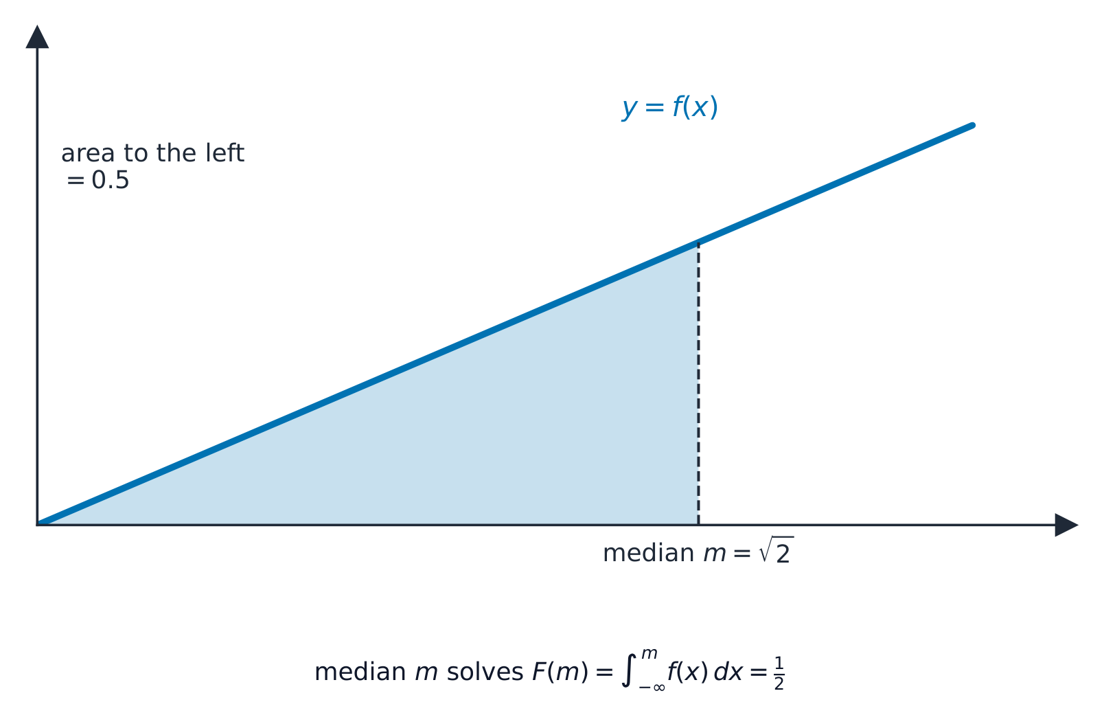
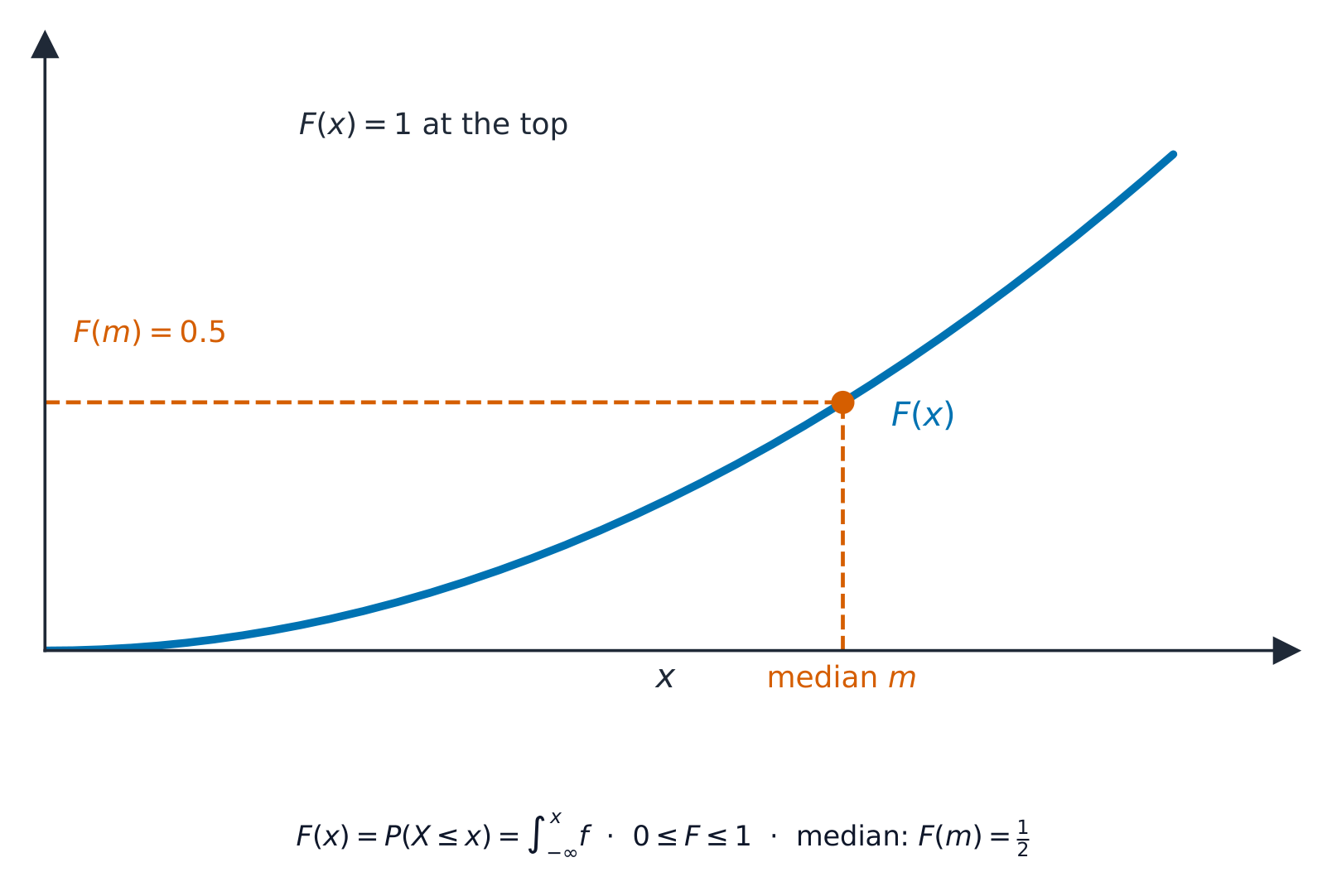
The cumulative distribution function 累积分布函数 $F(x) = P(X \leqslant x)$ is the running total: $F(x) = \displaystyle\int_{-\infty}^{x} f(t)\,dt$, and $f(x) = F'(x)$. Use $F$ to find probabilities and percentiles 百分位数 (for example, the median 中位数 solves $F(x) = 0.5$).

Worked example. A variable has $f(x) = \tfrac12 x$ for $0 \leqslant x \leqslant 2$. Find the median.

The cumulative distribution function is $F(x) = \displaystyle\int_0^x \tfrac12 t\,dt = \tfrac14 x^2$. Set $F(m) = 0.5$:

The distribution of a related variable. If $Y=g(X)$, find $Y$'s distribution through its cumulative function. For $Y=X^2$: $F_Y(y)=P(X^2\leqslant y)=P(-\sqrt y\leqslant X\leqslant\sqrt y)=F_X(\sqrt y)-F_X(-\sqrt y)$, then differentiate for $f_Y=F_Y'$. When $g$ is monotonic increasing there is a shortcut, $F_Y(y)=F_X\big(g^{-1}(y)\big)$.

Worked example. With $f_X(x)=\tfrac12 x$ on $[0,2]$ (so $F_X(x)=\tfrac14 x^2$), let $Y=X^2$. For $0\leqslant y\leqslant 4$, $F_Y(y)=F_X(\sqrt y)=\tfrac14 y$, so $f_Y(y)=F_Y'(y)=\tfrac14$ – that is, $Y$ is uniform on $[0,4]$.

When a sample is small and the population variance is unknown, base your hypothesis test 假设检验 on the $t$-distribution instead of the normal. The same idea gives a confidence interval 置信区间 for the mean:

where $t$ comes from the $t$-tables with $n - 1$ degrees of freedom. To compare two populations, use a two-sample (2-sample) or paired-sample $t$-test, after finding a pooled estimate 合并估计 of the shared variance when appropriate.

Worked example. A sample of $n = 10$ has mean $\bar{x} = 50$ and standard deviation $s = 4$. Find a $95\%$ confidence interval for the mean (use $t = 2.262$ for $9$ degrees of freedom).

A $\chi^2$-test (chi-squared test 卡方检验) compares observed counts $O$ with expected counts $E$ from a theoretical distribution 理论分布:

Compare this with a table value for the right number of degrees of freedom 自由度. Two uses: a goodness of fit 拟合优度 test (does the data follow the proposed model?), and a test for independence 独立性 of two variables in a contingency table 列联表.

Worked example. Four equally likely categories give observed counts $20, 30, 25, 25$ (so each expected count is $25$). Test the fit at the $5\%$ level.

With $4 - 1 = 3$ degrees of freedom the table value is $7.815$. Since $2 < 7.815$, do not reject the model.

A non-parametric test 非参数检验 makes no assumption that the data is normal, so it is useful when that assumption fails. The basic ones are:

• the sign test 符号检验: count how many values fall above and below a proposed median, and test those counts with a binomial model;
• the Wilcoxon signed-rank test 威尔科克森符号秩检验 (the matched-pairs test for paired data), which also uses the sizes of the differences, not just their signs;
• the Wilcoxon rank-sum test 威尔科克森秩和检验, for comparing two separate samples.

Worked example. Test whether a median is $5$. In a sample of $10$ values (none equal to $5$), $9$ lie above $5$ and $1$ lies below. Test at the $5\%$ level (two-tailed).

Under $H_0$ (median $= 5$) the number above follows $B(10, 0.5)$. The observed result ($9$ above) is extreme, so find $P(X \geq 9) = \binom{10}{9}(0.5)^{10} + (0.5)^{10} = \dfrac{11}{1024} = 0.0107$. For a two-tailed test compare with $\tfrac{1}{2}(5\%) = 0.025$. Since $0.0107 < 0.025$, reject $H_0$: there is evidence the median is not $5$.

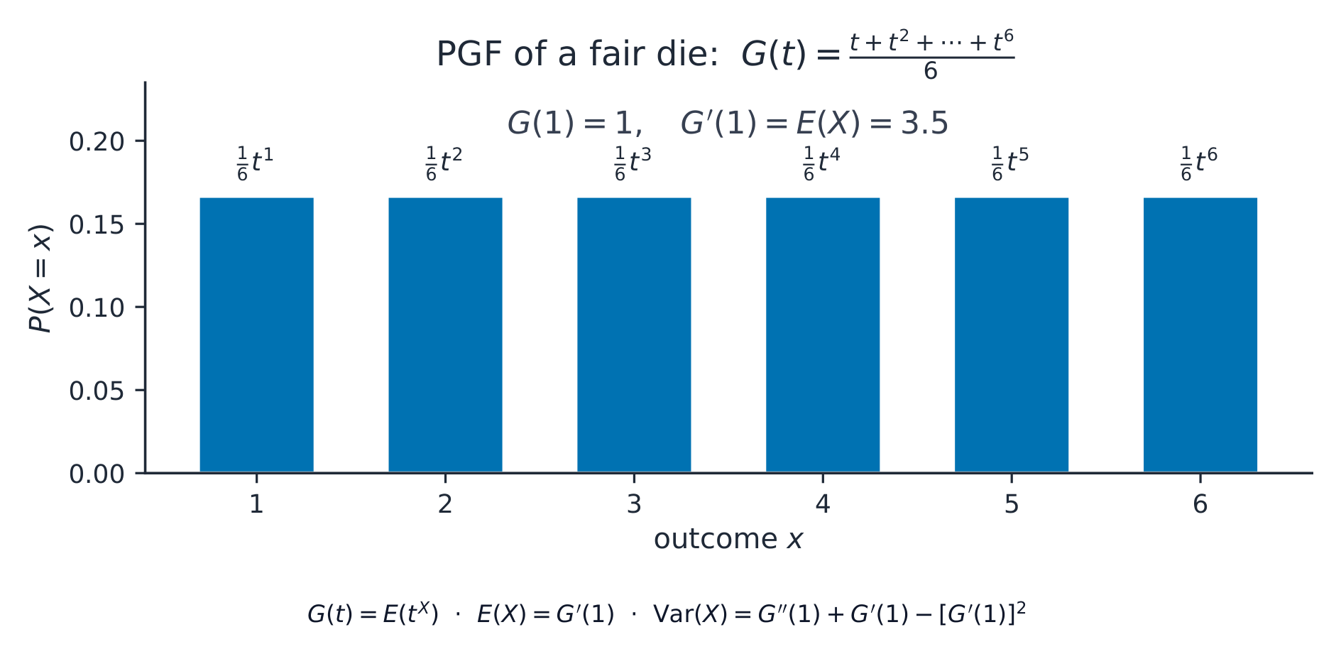
The probability generating function 概率母函数 of a discrete variable $X$ is

It packs the whole distribution into one function. The mean and variance come from its derivatives at $t = 1$: $E(X) = G'(1)$ and $\mathrm{Var}(X) = G''(1) + G'(1) - \big(G'(1)\big)^2$. Also, the PGF of a sum of independent variables is the product of their PGFs.

Worked example. $X$ has $P(X=0) = 0.5$, $P(X=1) = 0.3$, $P(X=2) = 0.2$. Find $E(X)$ using the PGF.

Here $G(t) = 0.5 + 0.3t + 0.2t^2$, so $G'(t) = 0.3 + 0.4t$ and

• For a continuous random variable, the pdf integrates to $1$ over its range, and $E(X) = \int x f(x)\,dx$.
• Use the $t$-distribution when the sample is small and the population variance is unknown; state the degrees of freedom.
• For a chi-squared test compute $\sum (O-E)^2/E$, compare with the critical value at the right degrees of freedom, and combine classes with $E < 5$.
• State $H_0$ and $H_1$ and give the conclusion in context for every test.