| Enduring Understanding | Learning Objective | Essential Knowledge |
|---|---|---|
VAR-1 | VAR-1.A |
|
探索单变量数据
AP 统计学 · 第 1 主题
 9:03
9:03
Exploring One-Variable Data
Measure the same thing twenty times and you will not get the same answer twenty times. Twenty students measure the same table. The values vary. That is not a…
英文讲解 · 内嵌中英文字幕
1.1
统计学导论:我们能从数据中学到什么?
大纲
来源:美国大学理事会 AP 课程与考试说明
统计学(statistics)是从数据(data)——从真实世界收集的数字或标签——中学习的科学。数据会变化,所以我们描述模式并考虑变异(variation),而不是期望每个值都相同。一个统计问题预期一个基于会变化的数据的答案。
有两个区分贯穿整个课程。参数(parameter)是整个总体的一个数值概括;统计量(statistic)是一个样本的数值概括——我们用统计量去估计无法直接测量的参数。而描述统计(descriptive statistics)只概括手头的数据集,推断统计(inferential statistics)则用一个样本对更大的总体做出并检验论断。
词汇表
训练
| 英文 | 中文 | 拼音 |
|---|---|---|
| Statistics/stəˈtɪstɪks/ | 统计学 | tǒng jì xué |
| data/ˈdeɪtə/ | 数据 | shù jù |
| variation/ˌveərɪˈeɪʃn/ | 变异 | biàn yì |
| parameter/pəˈræmɪtə/ | 参数 | cān shù |
| statistic/stəˈtɪstɪk/ | 统计量 | tǒng jì liàng |
| descriptive statistics/dɪˈskrɪptɪv stəˈtɪstɪks/ | 描述统计 | miáo shù tǒng jì |
| inferential statistics/ɪnfəˈrenʃl stəˈtɪstɪks/ | 推断统计 | tuī duàn tǒng jì |
1.2
变异的语言:变量
大纲
| Enduring Understanding | Learning Objective | Essential Knowledge |
|---|---|---|
VAR-1 | VAR-1.B |
|
VAR-1.C |
|
来源:美国大学理事会 AP 课程与考试说明
一个变量(variable)是一个能在个体之间不同的特征。两种:
- 分类(categorical)(定性):值是标签/组(眼睛颜色、品牌)。
- 定量(quantitative):值是你能做算术的数字(身高、年龄)。定量变量是离散(discrete)(可数)或连续(continuous)(测量)的。
选择正确的图和概括取决于你有哪一种。
探索
Categorical or quantitative?
Every variable is either categorical (it labels each unit with a group) or quantitative (a measured number you can average). Which kind it is decides the graphs and summaries you are allowed to use.
词汇表
训练
| 英文 | 中文 | 拼音 |
|---|---|---|
| variable/ˈveərɪəbl/ | 变量 | biàn liàng |
| Categorical/ˌkætɪˈɡɒrɪkl/ | 分类 | fēn lèi |
| Quantitative/ˈkwɒntɪteɪtɪv/ | 定量 | dìng liàng |
1.3
用表格表示分类变量
大纲
| Enduring Understanding | Learning Objective | Essential Knowledge |
|---|---|---|
UNC-1 | UNC-1.A |
|
UNC-1.B |
|
来源:美国大学理事会 AP 课程与考试说明
一个频数表(frequency table)列出每个类别的计数(count)(频数);一个相对频率(relative frequency)表列出每个类别的比例(proportion)(计数 ÷ 总数)。相对频率让你能公平地比较不同大小的组。
词汇表
训练
| 英文 | 中文 | 拼音 |
|---|---|---|
| frequency table/ˈfriːkwənsi ˈteɪbl/ | 频数表 | pín shuò biǎo |
| relative frequency/ˈrelətɪv ˈfriːkwənsi/ | 相对频率 | xiāng duì pín lǜ |
| proportion/prəˈpɔːʃn/ | 比例 | bǐ lì |
1.4
用图形表示分类变量
大纲
| Enduring Understanding | Learning Objective | Essential Knowledge |
|---|---|---|
UNC-1 | UNC-1.C |
|
UNC-1.D |
| |
UNC-1.E |
|
来源:美国大学理事会 AP 课程与考试说明
条形图(bar charts)把每个类别的计数或比例显示为分开的条;一个饼图(pie chart)显示每个类别在整体里的份额。条的高度(或扇区)让你能一眼比较类别。条可以按大小或按自然的类别顺序排列。
探索
Show a categorical variable as a pie chart
A pie chart turns each category's share of the whole into a slice: a bigger share is a bigger slice, and every slice together makes 100%. It is a picture of a relative-frequency table.
词汇表
训练
| 英文 | 中文 | 拼音 |
|---|---|---|
| Bar charts/bɑː tʃɑːts/ | 条形图 | tiáo xíng tú |
1.5
用图形表示定量变量
大纲
| Enduring Understanding | Learning Objective | Essential Knowledge |
|---|---|---|
UNC-1 | UNC-1.F |
|
UNC-1.G |
|
来源:美国大学理事会 AP 课程与考试说明
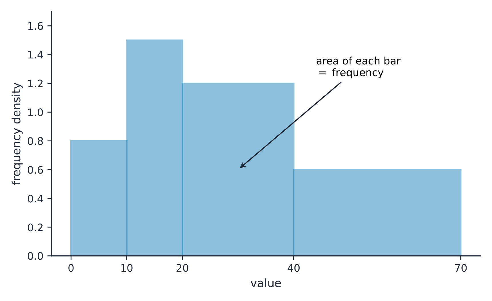
对于数字,用一个点图(dotplot)、茎叶图(stem-and-leaf plot),或直方图(histogram)(在称为区间的值区间上的条)。这些显示分布(distribution)——值如何散开。一个直方图的区间宽度改变图景,所以选择它以揭示形状。
探索
Explore how bin width shapes a histogram
A histogram groups data into equal-width bins and draws a bar over each. Change the bins and notice how the same data can look jagged (too narrow) or smooth (too wide) — the shape is a choice.
词汇表
训练
| 英文 | 中文 | 拼音 |
|---|---|---|
| dotplot/ˈdɒtplɒt/ | 点图 | diǎn tú |
| stem-and-leaf plot/stem ænd liːf plɒt/ | 茎叶图 | jīng yè tú |
| histogram/ˈhɪstəɡræm/ | 直方图 | zhí fāng tú |
| distribution/ˌdɪstrɪˈbjuːʃn/ | 分布 | fēn bù |
1.6
描述定量变量的分布
大纲
| Enduring Understanding | Learning Objective | Essential Knowledge |
|---|---|---|
UNC-1 | UNC-1.H |
|
来源:美国大学理事会 AP 课程与考试说明
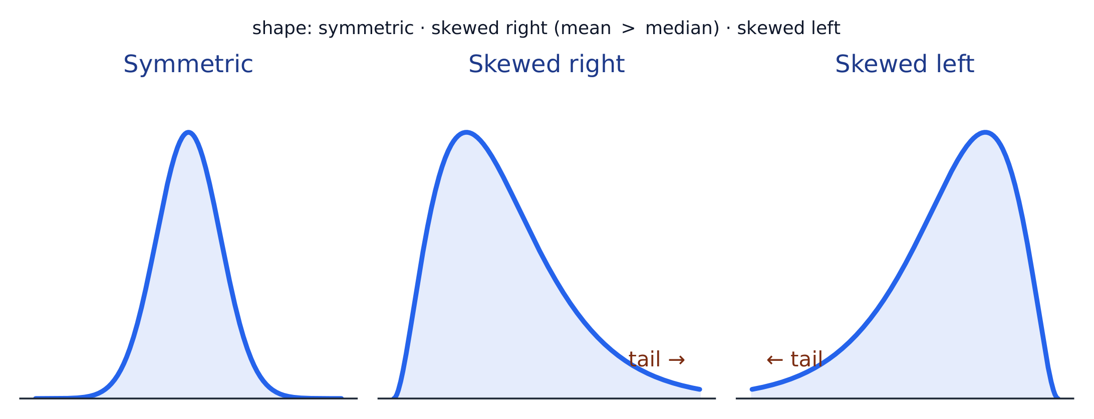
描述四件事(记住 SOCS):
- 形状(shape):对称,或偏斜(skewed)左/右(那一侧一条长尾),以及有多少个峰——一个主峰是单峰(unimodal),两个明显的峰是双峰(bimodal),各柱大致相等是均匀(uniform)。
- 离群值(outliers):远离其余的不寻常的值。
- 中心(center):一个典型的值(均值或中位数)。
- 散布(spread):值变化多少(范围、IQR、标准差)。
总是在上下文里、带单位地描述形状/中心/散布。
词汇表
训练
| 英文 | 中文 | 拼音 |
|---|---|---|
| Shape/ʃeɪp/ | 形状 | xíng zhuàng |
| skewed/skjuːd/ | 偏斜 | piān xié |
| unimodal/ˌʌnɪˈmɒdl/ | 单峰 | dān fēng |
| bimodal/baɪˈmɒdl/ | 双峰 | shuāng fēng |
| uniform/ˈjuːnɪfɔːm/ | 均匀 | jūn yún |
| Outliers/ˈaʊtlaɪəz/ | 离群值 | lí qún zhí |
1.7
定量变量的汇总统计量
大纲
| Enduring Understanding | Learning Objective | Essential Knowledge |
|---|---|---|
UNC-1 | UNC-1.I |
|
UNC-1.J |
| |
UNC-1.K |
|
来源:美国大学理事会 AP 课程与考试说明
- 中心: 均值(mean)$\bar{x}=\dfrac{\sum x_i}{n}$(平均)和中位数(median)(中间的值)。中位数抵抗离群值;均值被拉向偏斜。
- 散布: 范围(range)、四分位距(interquartile range)$\text{IQR}=Q_3-Q_1$(中间 50%),以及标准差(standard deviation)$s_x=\sqrt{\dfrac{\sum(x_i-\bar{x})^2}{n-1}}$(离均值的典型距离;它的平方是方差(variance))。
- 五数概括(five-number summary):min、$Q_1$、中位数、$Q_3$、max。
对偏斜数据用抵抗性(resistant)测度(中位数、IQR);对大致对称的数据用均值和标准差。
一个值的百分位数(percentile)是数据中在它或以下的百分比——所以中位数是第 50 百分位数,$Q_1$ 是第 25。一个累积相对频率图(cumulative relative frequency graph)让百分位数容易读出:对每个值它画出数据中在它或以下的比例,从 0 上升到 1。从一个值向上到曲线再横过去到它的百分位数,或反过来找一个给定百分位数处的值(同样的读法对一张累积频率表也有效)。
Worked example. 对于数据 $4, 8, 6, 10, 7$:均值是 $\bar{x}=\dfrac{4+8+6+10+7}{5}=\dfrac{35}{5}=7$。排序到 $4,6,7,8,10$,中位数是中间的值,$7$。这里均值和中位数一致,因为数据大致对称。
词汇表
训练
| 英文 | 中文 | 拼音 |
|---|---|---|
| mean/miːn/ | 均值 | jūn zhí |
| median/ˈmiːdiːən/ | 中位数 | zhōng wèi shù |
| interquartile range/ˌɪntəˈkwɔːtaɪl reɪndʒ/ | 四分位距 | sì fēn wèi jù |
| standard deviation/ˈstændəd ˌdiːvɪˈeɪʃn/ | 标准差 | biāo zhǔn chà |
| variance/ˈveərɪəns/ | 方差 | fāng chà |
| five-number summary/faɪv ˈnʌmbə ˈsʌməri/ | 五数概括 | wǔ shù gài kuò |
| percentile/pəˈsentaɪl/ | 百分位数 | bǎi fēn wèi shù |
| cumulative relative frequency graph/ˈkjuːmjʊlətɪv ˈrelətɪv ˈfriːkwənsi ɡræf/ | 累积相对频率图 | lěi jī xiāng duì pín lǜ tú |
1.8
汇总统计量的图形表示
大纲
| Enduring Understanding | Learning Objective | Essential Knowledge |
|---|---|---|
UNC-1 | UNC-1.L |
|
UNC-1.M |
|
来源:美国大学理事会 AP 课程与考试说明
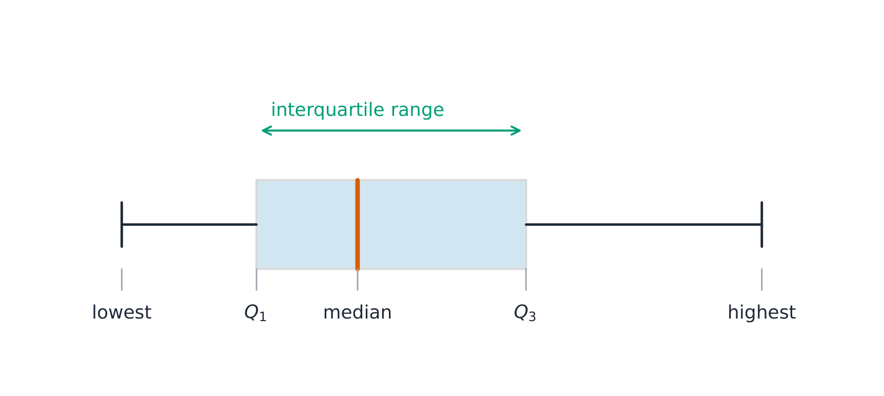
一个箱线图(boxplot)画五数概括:一个从 $Q_1$ 到 $Q_3$、中位数在里面的箱,以及到最极端的非离群值的须。一个点是一个离群值,若它落在一个四分位数之外超过 $1.5\times\text{IQR}$ ——一个你可能被要求应用的规则。箱线图对并排比较几个组很理想。
Worked example. 一个数据集有 $Q_1=20$ 和 $Q_3=32$,所以 $\text{IQR}=12$。离群值围栏是 $Q_1-1.5(12)=2$ 和 $Q_3+1.5(12)=50$。任何低于 $2$ 或高于 $50$ 的值被标记为一个离群值。

探索
Explore the five-number summary as a boxplot
Drag $Q_1$, the median, and $Q_3$ to see the box (its length is the IQR) and how the median's position inside the box reveals skew — a median close to $Q_1$ signals a right-skewed distribution.
词汇表
训练
| 英文 | 中文 | 拼音 |
|---|---|---|
| boxplot/ˈbɒksplɒt/ | 箱线图 | xiāng xiàn tú |
1.9
比较定量变量的分布
大纲
| Enduring Understanding | Learning Objective | Essential Knowledge |
|---|---|---|
UNC-1 | UNC-1.N |
|
UNC-1.O |
|
来源:美国大学理事会 AP 课程与考试说明
要比较两个或更多组,比较形状、中心和散布,并提及离群值——总是用比较性词语("A 组有一个更高的中位数比 B 组")并在上下文里。不要只是分别描述每个组;把比较显式化。
探索
Compare distributions with box plots
A box plot draws the five-number summary. Placing two box plots on the same scale compares their centre (median), spread (IQR = box width) and skew at a glance — the fair way to compare groups.
1.10
正态分布
大纲
| Enduring Understanding | Learning Objective | Essential Knowledge |
|---|---|---|
VAR-2 | VAR-2.A |
|
VAR-2.B |
| |
VAR-2.C |
|
来源:美国大学理事会 AP 课程与考试说明
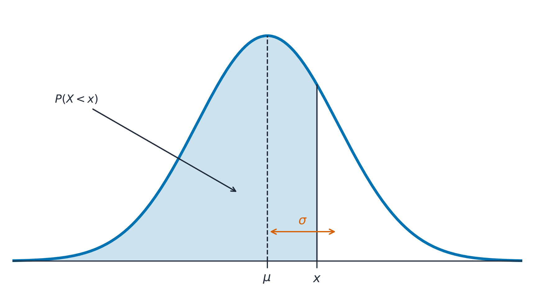
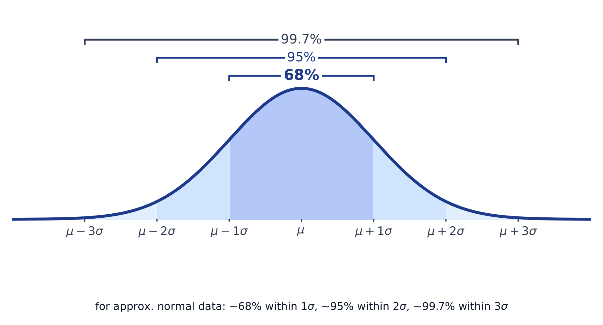
一个正态分布(normal distribution)是一个由它的均值 $\mu$ 和标准差 $\sigma$ 描述的对称、钟形模型。经验法则(empirical rule)(68–95–99.7):约 68% 的值落在离均值 $1\sigma$ 内、95% 在 $2\sigma$ 内,而 99.7% 在 $3\sigma$ 内。
一个**$z$ 分数**(z-score)测量一个值离均值多少个标准差:
$$z=\frac{x-\mu}{\sigma}.$$
转换成一个 $z$ 分数,然后用正态表或技术求以下的、以上的,或之间的比例(面积)——并反转这个过程以从一个给定百分位数求一个值。
Worked example. 测验分数是正态的,$\mu=500$ 和 $\sigma=100$。一个 $700$ 的分数有 $z=\dfrac{700-500}{100}=2$。由经验法则,$95\%$ 的分数落在 $2\sigma$ 内,所以 $2.5\%$ 落在 $700$ 以上——意味着一个 $700$ 大约在第 $97.5$ 百分位。
探索
Explore area under the normal curve
The proportion of data below a value equals the area under the curve to its left. Shade a tail or a central band to see the 68–95–99.7 empirical rule and read a $z$-score as an area.
词汇表
训练
| 英文 | 中文 | 拼音 |
|---|---|---|
| normal distribution/ˈnɔːml ˌdɪstrɪˈbjuːʃn/ | 正态分布 | zhèng tài fēn bù |
| empirical rule/emˈpɪrɪkl ruːl/ | 经验法则 | jīng yàn fǎ zé |
| $z$-score/ˈzed skɔː/ | 标准分数 | biāo zhǔn fēn shù |
1.10
考试技巧
- 用形状、中心、散布和离群值(SOCS)描述一个分布——总是在上下文里。
- 均值被离群值拉动;中位数抵抗它们,所以对偏斜数据首选中位数。
- 对一个正态分布用 68–95–99.7 法则和 z 分数 $z=\tfrac{x-\mu}{\sigma}$。
- 用并排箱线图比较分布并评论中心、散布和形状。
- 标准差测量离均值的一个典型距离;IQR 与中位数配对。
本主题的互动课程
逐步学习,并即时检测练习。