AP Physics C: Electricity and Magnetism is the calculus-based electromagnetism course: charges, fields and Gauss's law; electric potential; conductors and capacitors; circuits; magnetic fields; and electromagnetic induction. It is usually taken after Mechanics and assumes that level of calculus.
Gauss's law and Ampère's law decide how this course feels. Both are really about choosing a surface or loop that makes the integral trivial — a skill you build by doing many, not by reading the law. Symmetry is the whole game.
Induction questions punish sign errors more than anything else, so fix one convention for flux direction and use it every time.
Notes cover Gauss's law through to Maxwell's equations, unit by unit, with the vector calculus written out. The library carries the released FRQs; the hardest marks in E&M go to choosing the right symmetry before integrating, so the examples start there.
학습 목표 8.1.A: 전하를 띤 물체나 시스템 간의 상호작용으로 인해 발생하는 전기력을 설명한다.
8.1.A.1 전하는 모든 물질의 근본적인 성질이다.
8.1.A.1.i 전하는 스칼라량이며 양(+), 음(-)으로 서술된다.
8.1.A.1.ii 단일 전자 또는 양성자의 전하 크기인 기본 전하 $e$은 분할할 수 없는 최소 전하량으로 간주할 수 있다.
8.1.A.1.iii 전자의 전하량은 $-e$이고 양성자의 전하량은 $+e$이며, 중성자는 전기적 전하를 가지지 않는다.
8.1.A.1.iv 점전하는 분석 대상 상황의 맥락에서 전하를 띤 물체나 시스템의 물리적 크기가 무시할 수 있을 정도로 작다고 가정하는 모델이다.
8.1.A.2 쿨롱의 법칙은 두 전하를 띤 물체 사이의 정전기력이 각 전하의 크기에 비례하고, 물체 사이의 거리의 제곱에 반비례함을 설명한다.
관련 식:$\left| \vec{F}_E \right| = \dfrac{1}{4\pi\varepsilon_0} \dfrac{|q_1 q_2|}{r^2} = k \dfrac{|q_1 q_2|}{r^2}$
8.1.A.3 정전기력의 방향은 상호작용하는 물체의 전하 부호에 따라 결정되며, 물체 사이의 분리 선상(직선)을 따라 작용한다.
8.1.A.3.i 동일한 부호의 전하를 띤 두 물체는 서로 밀어내는斥力를 발생시킨다.
8.1.A.3.ii 서로 다른 부호의 전하를 띤 두 물체는 서로 끌어당기는引力를 발생시킨다.
8.1.A.4 전기력은 일상 경험에서 물체의 일부anganscopic 특성에 관여한다. 그러나 많은 입자 상호작용이 일어나기 때문에, 일상적인 힘은 정상력, 마찰력, 장력 등의 비근본력인 접촉력으로 처리하는 것이 더 편리하다.
학습 목표 8.1.B: 질량을 가진 전하를 띤 물체 간의 상호작용으로 인해 발생하는 전기력과 중력来说明。
8.1.B.1 정전기력은 끌거나 밀 수 있지만, 중력은 항상 끌림 force이다.
8.1.B.2 질량과 전기 전하를 가진 두 물체에 대해, 중력의 크기는 일반적으로 전기력의 크기보다 훨씬 작다.
8.1.B.3 중력은 전기력보다 약하지만 거시적 규모에서는 중력이 지배적으로 작용하는데, 이는 거시적 규모의 시스템이 전기적으로 중성(중성전하 상태)을 이루기 때문이다.
학습 목표 8.1.C: 물질이나 매질의 전기유전율来说明。
8.1.C.1 전기유전율은 물질이나 매질이 전기장 내에서 극화되는 정도를 측정하는 값이다.
8.1.C.2 전기 극화는 외부 전기장에 의해 전자들이 재배열되는 것으로 모델링되며, 이로 인해 물질이나 매질 내부에 양전하와 음전하의 분리가 발생한다.
8.1.C.3 진공은 물리적 관계식에 나타나는 일정한 값의 전기유전율 $\varepsilon_0$을 가진다.
8.1.C.4 물질의 유전율은 진공의 값과 다르며, 이는 물질의 구성 및 배치에 기인한다.
8.1.C.4.i 특정 물질에서 전기유전율은 해당 물질 내에서 전자가 배치 상태를 변경하기 쉬운 정도에 의해 결정된다.
8.1.C.4.ii 도체는 전하 운반체가 쉽게 이동할 수 있는 전기적으로 전도성 있는 소재로 만들어지며, 절연체는 전하 운반체가 쉽게 이동할 수 없는 전기적으로 비전도성 있는 소재로 만들어진다.
경계 문구: AP Physics C: 전기&자기 과목에서는 학생이 네 개 이하의 상호작용 전하를 띤 물체 또는 시스템 간의 전기력을 계산하는 것만을 요구한다. 대칭성이 높은 상황에서는 더 많은 전하로부터의 resultant 전기력 분석은 허용된다. 단, 8.4과 8.6 주제에서 기술된 바와 같이 전하 분포에 대한 전기장을 계산하는 것은 학생에게 요구됨을 유의하라.
출처: College Board AP Course and Exam Description
Electric charge 电荷 comes in positive and negative; like charges repel, opposites attract. Charge is quantized 量子化 – every charge is a whole-number multiple of the elementary charge 基本电荷$e=1.6\times10^{-19}\ \text{C}$ – and obeys conservation of charge 电荷守恒: charge is never created or destroyed, only moved. The force between two point charges 点电荷 is Coulomb's law 库仑定律:
an inverse-square 平方反比 force along the line joining them, with $\dfrac{1}{4\pi\varepsilon_0}=k=9.0\times10^{9}\ \text{N}\cdot\text{m}^2/\text{C}^2$. For several charges (AP uses four or fewer, unless symmetry helps), add the force vectors on the charge you care about – superposition 叠加.
Charge is a fundamental property 基本属性 of matter, and a point charge is a model that ignores the size of a charged object. The constant $\varepsilon_0$ is the permittivity of free space 真空介电常数 – a material property of the vacuum. The permittivity of matter differs from $\varepsilon_0$, set by how easily the material polarizes, which is why a dielectric between charges weakens the force. Note too that although the electric force is far stronger than gravity, gravity dominates at astronomical scales because large bodies are nearly neutral.
Worked example. Two $+2.0\ \mu\text{C}$ charges sit $0.30\ \text{m}$ apart: $F=\dfrac{kq_1q_2}{r^2}=\dfrac{9.0\times10^{9}(2.0\times10^{-6})^2}{(0.30)^2}=0.40\ \text{N}$, repulsive.
Worked example (vectors). Charges $+3.0\ \mu\text{C}$ and $-3.0\ \mu\text{C}$ sit at two corners of a right angle, each $0.30\ \text{m}$ from a $+1.0\ \mu\text{C}$ charge at the corner. Each exerts $F=\dfrac{(9.0\times10^{9})(3.0\times10^{-6})(1.0\times10^{-6})}{0.09}=0.30\ \text{N}$ – one a push, one a pull, at right angles to each other. The net force is $F_{\text{net}}=\sqrt{0.30^2+0.30^2}=0.42\ \text{N}$, pointing between them. Never add magnitudes blindly: components first.
탐색하기
전하 소스의 전기장(field) 탐구하기
전하의 **부호와 크기(sign and size)**를 변경하세요. 전기장 선은 양전하에서 바깥쪽으로 향하고 음전하로 들어옵니다. 전하 근처에서 $1/r^2$ 선들의 밀집은 쿨롱의 힘이 거리와 함께 $F = k\,|q_1 q_2|/r^2$ 약해지는 이유를 보여줍니다.
permittivity of free space/ˌpɜːmɪˈtɪvəti ɒv friː speɪs/
진공 투과율
8.2
Electric Charge and the Process of Charging
Syllabus
학습 목표 8.2.A: 전하 보존 법칙을 사용하여 시스템의 거동을 설명한다.
8.2.A.1 시스템의 순전하 또는 전하 분포는 다른 시스템의 순전하 또는 전하 분포의 존재 또는 변화에 따라 변할 수 있다.
8.2.A.1.i 시스템 간의 마찰이나 접촉으로 인해 시스템의 순전하가 변할 수 있다.
8.2.A.1.ii 유도 전하 분리는 두 시스템 간의 정전기력이 시스템 내 전하 분포를 변경하여 하나 또는 두 시스템 모두의 극화를 유발할 때 발생한다.
8.2.A.1.iii 중성 시스템에서도 유도된 전하 분리가 발생할 수 있다.
8.2.A.2 시스템의 순전하 변화는 시스템과 주변 환경 간의 전하 이동에 기인한다.
8.2.A.2.i 시스템의 충전은 일반적으로 전자들이 시스템 안팎으로 이동하는 것을 포함한다.
8.2.A.2.ii 시스템으로의 전하 이동이나 시스템으로부터의 전하 이송이 없으면 시스템의 순전하는 일정하게 유지된다.
8.2.A.3 접지(그라운드)란 전하를 띤 물체를 훨씬 크고 거의 중성인 시스템(예: 지구)에 전기적으로 연결하는 것이다.
출처: College Board AP Course and Exam Description
A conductor 导体 lets charge move freely; an insulator 绝缘体 holds it in place. Objects gain net charge three ways:
Charging by friction 摩擦起电: rubbing transfers electrons from one surface to the other.
Charging by conduction 传导起电: touching a charged object shares charge of the same sign.
Charging by induction 感应起电: a nearby charge pushes the conductor's charge apart; ground 接地 the far side, remove the ground wire first, and the conductor is left with the opposite sign – all without contact.
An insulator cannot pass charge, but it can develop polarization 极化: its molecules stretch or turn so one face is slightly positive and the other slightly negative. That is why a charged comb picks up neutral paper scraps. An electroscope 验电器 shows net charge by its leaves repelling; on any isolated conductor the excess charge sits entirely on the outer surface.
탐색하기
마찰에 의한 충전过程(charging by rubbing) 탐구하기
마찰은 **전자(electrons)**를 물체에 전달하여 물체를 음전하로 만듭니다. 충전된 물체는 중성 벽이나 머리카락을 극화(polarization)로 끌어당기지만, 다른 같은 부하의 물체에는 밀어냅니다. 이는 마찰, 도통, 유도의 모든 충전 과정에서 발생하는 전자 이동과 같습니다.
8.3.A.2.i A test charge is a point charge of small enough magnitude such that its presence does not significantly affect an electric field in its vicinity.
8.3.A.2.ii An electric field points away from isolated positive charges and toward isolated negative charges.
8.3.A.2.iii The electric force exerted on a positive test charge by an electric field is in the same direction as the electric field.
8.3.A.3 The electric field is a vector quantity and can be represented in space using vector field maps.
8.3.A.3.i The net electric field at a given location is the vector sum of individual electric fields created by nearby charged objects.
8.3.A.3.ii Electric field maps use vectors to depict the magnitude and direction of the electric field at many locations within a given region.
8.3.A.3.iii Electric field line diagrams are simplified models of electric field maps and can be used to determine the relative magnitude and direction of the electric field at any position in the diagram.
8.3.B
Describe the electric field generated by charged conductors or insulators.
8.3.B.1 While in electrostatic equilibrium, the excess charge of a conductor is distributed on the surface of the conductor, and the electric field within the conductor is zero.
8.3.B.1.i At the surface of a charged conductor, the electric field is perpendicular to the surface.
8.3.B.1.ii The electric field outside an isolated sphere with spherically symmetric charge distribution is the same as the electric field due to a point charge with the same net charge as the sphere located at the center of the sphere.
8.3.B.2 While in electrostatic equilibrium, the excess charge of an insulator is distributed throughout the interior of the insulator as well as at the surface, and the electric field within the insulator may have a nonzero value.
출처: College Board AP Course and Exam Description
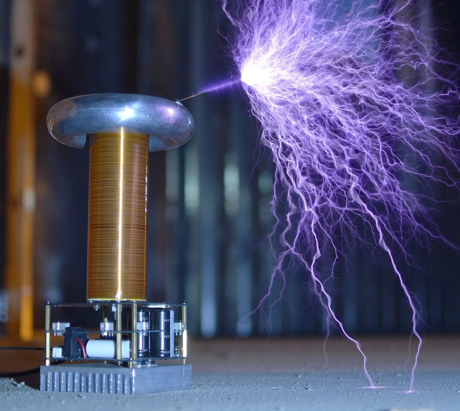
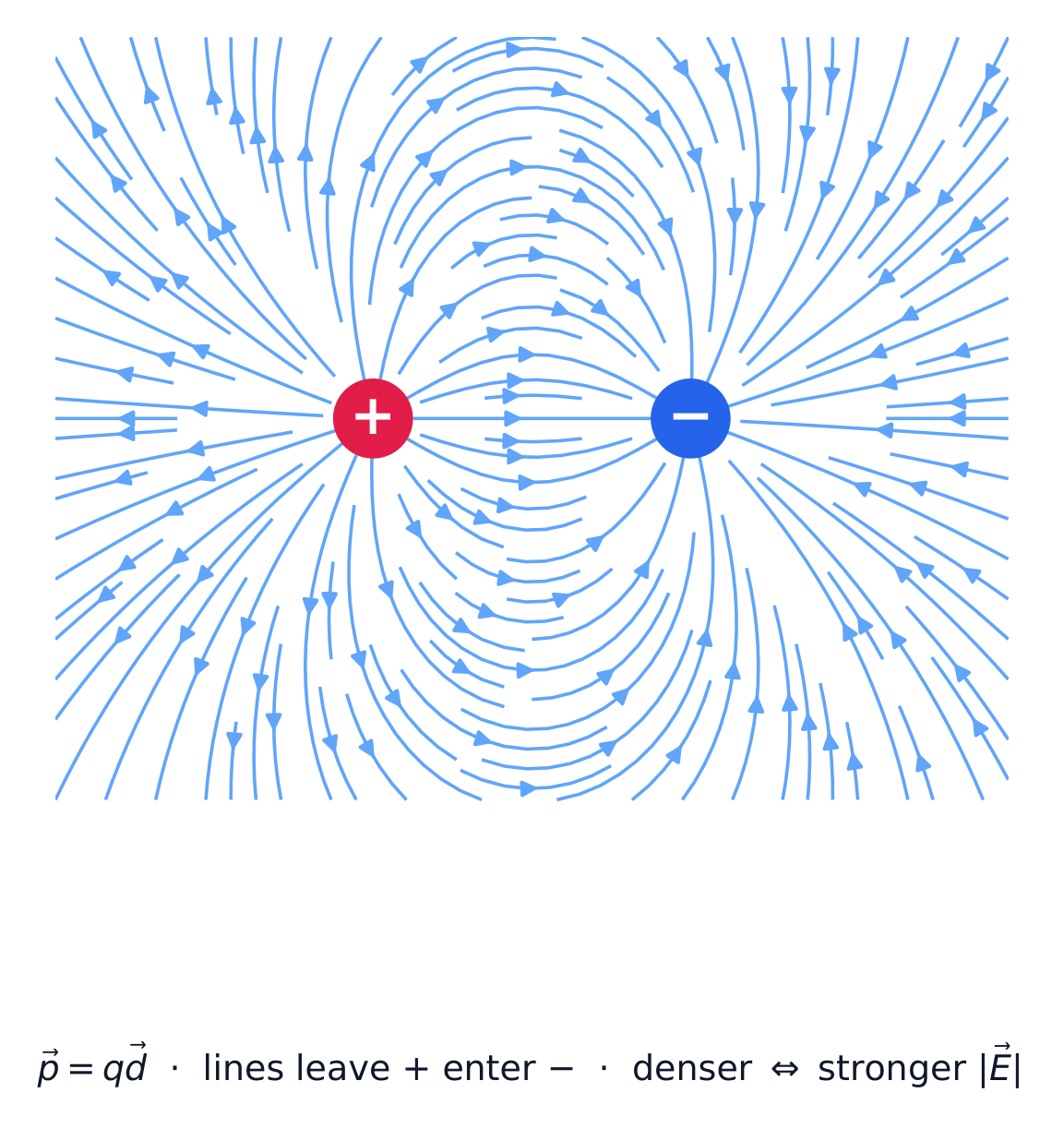
The electric field of a dipoleA Tesla coil throws sparks: it raises the voltage so high that the electric field ionizes the surrounding air, and charge leaps across as a visible discharge
The electric field 电场 at a point is the force per unit charge that a small positive test charge 检验电荷 would feel there:
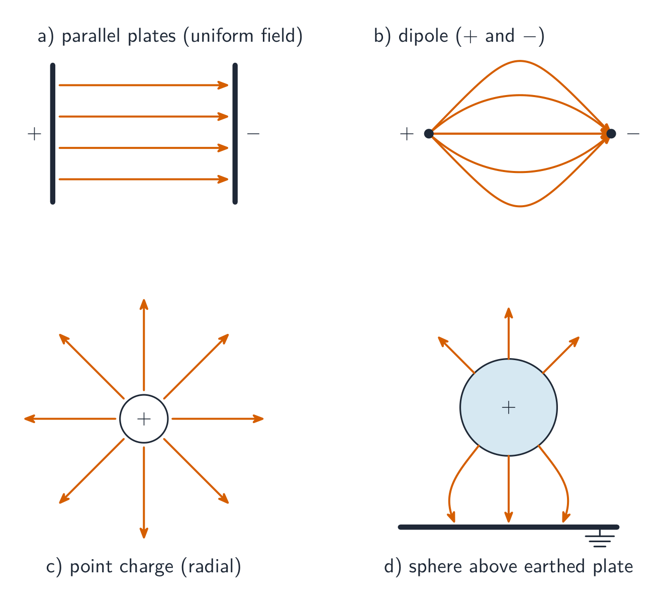
A charge placed in a field feels $\vec{F}=q\vec{E}$ – positive charges along the field, negative charges against it. Fields from several sources add as vectors (superposition again). Field lines 电场线 make the field visible: they point away from positive charge and toward negative, their density shows the strength, and they never cross.
Electric field-line patterns for parallel plates, a dipole, and a point chargeElectric field lines of a dipole point from the positive to the negative charge
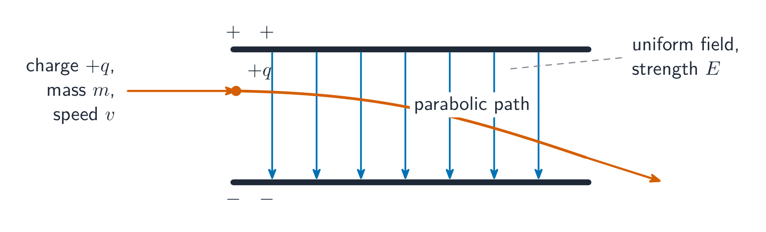
In a uniform 均匀 field a charge feels a constant force, so it accelerates uniformly – launched sideways, it follows a parabola, just like a projectile in gravity.
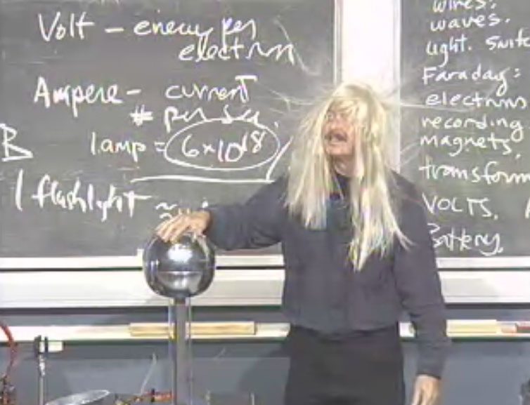
A charge crossing a uniform field follows a parabolic pathCharge spreads over the dome and onto the hair; like charges repel, so the strands push apart
탐색하기
점전하(point charge)의 전기장 선 탐구하기
전하를 양수 또는 음수로 설정하세요. 전기장 선은 양전하에서 시작하여 음전하에서 끝납니다. 서로 교차하지 않으며, $\vec{E}$가 가장 강한 곳에서 선들이 빽빽해집니다. 선의 밀도는 전기장 세기에 비례합니다.
8.4.A.1 특정 전하 분포에 대한 전기장의 식은 적분 및 중첩 원리를 이용하여 얻을 수 있다.
관련 식:$\vec{E} = \dfrac{1}{4\pi\varepsilon_0} \displaystyle\int \dfrac{dq}{r^2} \hat{r}$
8.4.A.2 특정 전하 분포의 대칭성을 고려하면 해당 분포에서 발생하는 전기장 분석을 간소화할 수 있다.
경계 statement: AP Physics C: Electricity & Magnetism에서는 다음 전하 분포 및 위치에서 calculus를 사용하여 전기장을 구하는 것만要求学生: 중심 축으로부터 거리 있는 무한히 긴 균일 전하선 또는 실린더, 링 축 상의 위치にある 얇은 전하 링, 반원 호 또는 반원 호의 일부의 중심, 그리고 직선 전하와 일렬인 지점이나 수직 이등분선 상의 위치 있는 유한 전하선 또는 선전하.
출처: College Board AP Course and Exam Description
For a continuous charge distribution 连续电荷分布, cut the object into pieces $dq$ and integrate their point-charge fields:
Write $dq$ using the right density: $\lambda\,dl$ with the linear charge density 线电荷密度 (a line or ring), $\sigma\,dA$ with the surface charge density 面电荷密度, or $\rho\,dV$ with the volume charge density 体电荷密度. Then use symmetry 对称性 to cancel components before integrating – that sentence is usually a scored step. AP's calculus cases: a finite line (collinear point or perpendicular bisector), an infinite wire or cylinder, a ring on its axis, and an arc at its centre.
Worked example (ring, on axis). A ring of radius $R$ carries charge $Q$. At a point $z$ along the axis, each element is a distance $\sqrt{R^2+z^2}$ away, and by symmetry the sideways components cancel, leaving only the axial part ($\cos\alpha=z/\sqrt{R^2+z^2}$):
8.5.A
Describe the electric flux through an arbitrary area or geometric shape.
8.5.A.1 Flux describes the amount of a given quantity that passes through a given area.
8.5.A.2 For an electric field $\vec{E}$ that is constant across an area $\vec{A}$, the electric flux through the area is defined as $\Phi_E = \vec{E} \bullet \vec{A}$.
8.5.A.2.i The direction of the area vector is defined as perpendicular to the plane of the surface and outward from a closed surface.
8.5.A.2.ii The sign of flux is given by the dot product of the electric field vector and the area vector.
8.5.A.3 The total electric flux passing through a surface is defined by the surface integral of the electric field over the surface.
Electric flux 电通量 measures how much field passes through a surface:
$$\Phi_E=\int \vec{E}\cdot d\vec{A}.$$
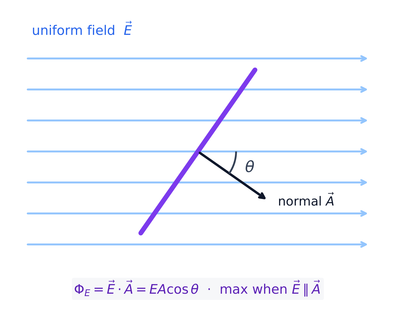
For a uniform field through a flat area, $\Phi_E=EA\cos\theta$, where the area vector 面积矢量 is perpendicular to the surface. Flux is positive where field lines exit a closed surface and negative where they enter – only the perpendicular component of $\vec{E}$ counts.
Electric flux through a surface depends on the angle between the field and the surface normal
8.6.A.1 가우스의 법칙은 가우스曲面을 통과하는 전기 플럭스와 해당曲面에 포획된 전하 사이의 관계를 나타낸다.
관련 식:$\Phi_E = \dfrac{q_{\text{enc}}}{\varepsilon_0}$ 및 $\displaystyle\oint \vec{E} \cdot d\vec{A} = \dfrac{q_{\text{enc}}}{\varepsilon_0}$
8.6.A.2 가우스曲面은 3차원 폐곡면이다.
8.6.A.3 포획된 전하량이 일정할 경우, 가우스曲面을 통과하는 총 전기 플럭스는 가우스曲面의 크기에 의존하지 않는다.
8.6.A.4 가우스曲面은 통상적으로 포획된 전하가 만든 전기장이曲面의 서로 다른 영역에 대해 수직이거나 평행하도록 설계되어,曲面 적분을 단순화하는 결과를 얻기 위해 구성된다.
8.6.A.5 전하 밀도 함수가 주어진 경우, 총 전하는 전하 분포의 길이(1차원), 면적(2차원) 또는 부피(3차원)에 대해 전하 밀도를 적분하여 구할 수 있습니다. 예를 들어: $Q_{\text{total}} = \displaystyle\int \rho(\vec{r})\, dV$
8.6.A.6 맥스웰 방정식은 전자기학을 완전히 기술하는 일련의 방정식입니다. 가우스 법칙은 맥스웰의 첫 번째 방정식입니다.
관련 식:$\displaystyle\oint \vec{E} \cdot d\vec{A} = \dfrac{q_{\text{enc}}}{\varepsilon_0}$
경계 문구: AP Physics C: 전기 및 자기 과목에서는 학생이 가우스 법칙을 점전하 및 구형, 원통형 또는 평면 대칭성을 가진 전하 분포에 정량적으로 적용하도록 요구합니다.
출처: College Board AP Course and Exam Description
Gauss's law 高斯定律 – the first of Maxwell's equations – relates the flux through any closed surface to the charge inside it:
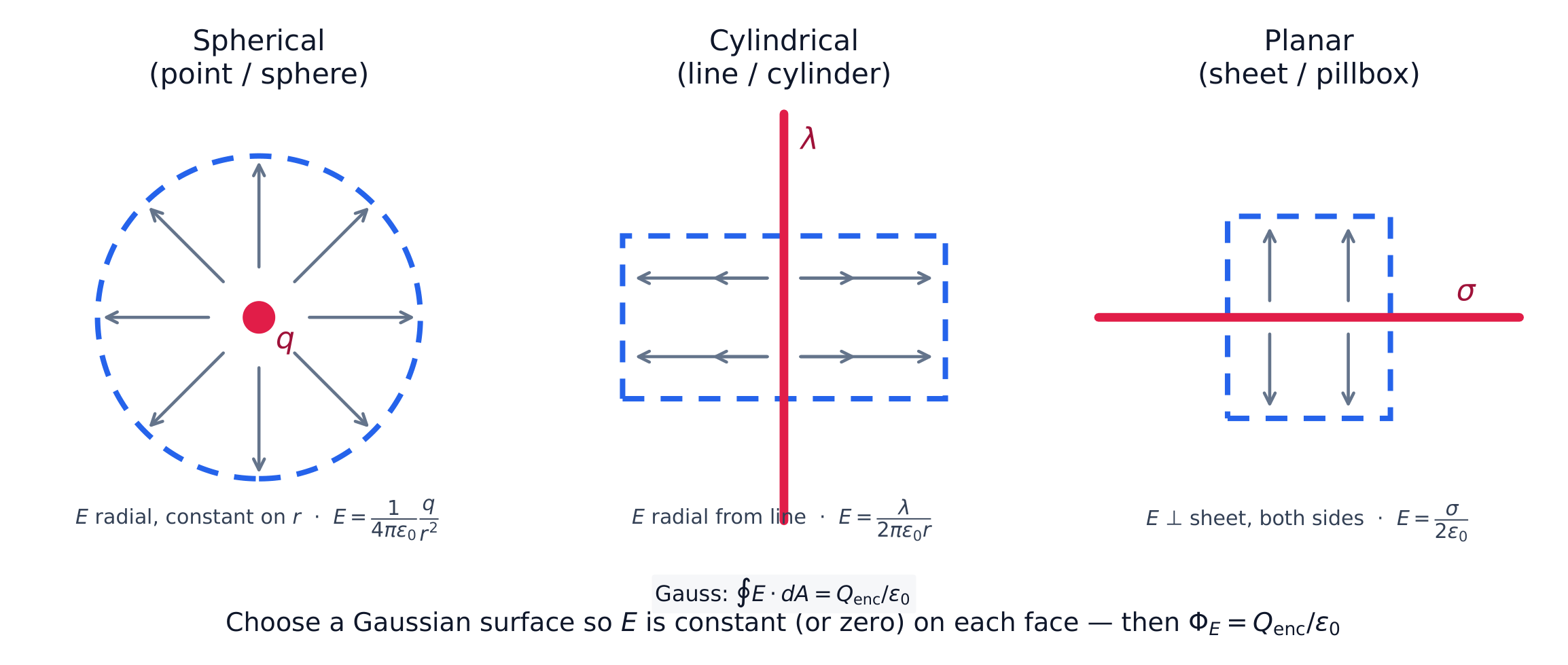
It is true for any closed surface, but it solves for $E$ only when symmetry lets you choose a Gaussian surface 高斯面 on which $E$ is constant and perpendicular (or parallel, contributing zero). The three symmetries AP tests: spherical symmetry 球对称 (concentric sphere), cylindrical symmetry 柱对称 (coaxial cylinder), and planar symmetry 平面对称 (a straddling "pillbox").
A Gaussian surface is chosen to match the symmetry of the charge
Worked example (sphere). Outside a sphere of total charge $Q$, a spherical Gaussian surface of radius $r$ gives $E(4\pi r^2)=Q/\varepsilon_0$, so $E=\dfrac{kQ}{r^2}$ – identical to a point charge at the centre. Inside a uniformly charged solid sphere of radius $R$, the surface encloses only $Q_{\text{enc}}=Q\,r^3/R^3$, so $E=\dfrac{kQr}{R^3}$: zero at the centre, growing linearly to the surface.
Worked example (wire). For an infinite wire with charge per length $\lambda$, take a coaxial cylinder of radius $r$ and length $L$. The ends contribute nothing ($\vec{E}\perp d\vec{A}$), so $E(2\pi rL)=\dfrac{\lambda L}{\varepsilon_0}$ and $E=\dfrac{\lambda}{2\pi\varepsilon_0 r}$. The same pillbox method gives an infinite sheet's field, $E=\dfrac{\sigma}{2\varepsilon_0}$, uniform on both sides.
Exam skill. A full-credit Gauss's-law answer has four parts: name the surface, state the symmetry argument (why $E$ is constant and perpendicular on it), count $Q_{\text{enc}}$, then solve. Skipping the symmetry sentence loses the reasoning point – and remember Gauss's law also explains why $E=0$ inside any conductor in equilibrium.
$U_E$ is defined as the work an external force must do to bring the charges from infinitely far away to a distance $r$ apart. The signs carry the physics:
Like charges:$U_E>0$. An outside push was needed to bring them together. If released, they fly apart, and the stored energy becomes kinetic energy 动能.
Opposite charges:$U_E<0$. The pair is bound. You must supply $|U_E|$ of work to pull them apart to infinity.
The electric force is a conservative force 保守力: the work it does depends only on the start and end points, not the path, and equals $-\Delta U_E$.
For a system 系统 of several charges, add the potential energy of every distinct pair:
Worked example. Three $+2.0\ \mu\text{C}$ charges sit at the corners of an equilateral triangle with sides $0.30\ \text{m}$. Each pair stores $U=\dfrac{kq^2}{r}=\dfrac{(9.0\times10^{9})(2.0\times10^{-6})^2}{0.30}=0.12\ \text{J}$. There are three pairs, so $U_{\text{total}}=3\times0.12\ \text{J}=0.36\ \text{J}$. This is the work needed to assemble the triangle from infinity – and the kinetic energy the charges would share if all three were released.
9.2.A.3 두 점 사이의 전기포텐셜 차이는 시험 전하가 두 점 사이를 이동할 때 단위 전하당 전기포텐셜 에너지의 변화량입니다.
식:$\Delta V = \dfrac{\Delta U_E}{q}$
9.2.A.4 전기포텐셜 차이는 배터리와 같이 양전하와 음전하를 분리시키는 화학 과정에 의해 발생할 수도 있습니다.
경계 문구: AP Physics C: 전기 및 자기 과목에서는 다음 전하 분포와 위치에 대한 전기포텐셜을 찾기 위해 미적분을 사용하도록要求学生: 중심 축으로부터 거리인 무한히 긴 균일하게 충전된 선 또는 원통, 링 축상의 위치인薄薄的电荷环, 반원 호 또는 반원 호 일부의 중심, 선전하와 공선상에 있는 점 또는 수직 이등분선상의 위치인 유한한 선 또는 선전하.
학습 목표 9.2.B: 전기포텐셜과 전기장 사이의 관계를 설명하십시오.
9.2.B.1 특정 위치에서 임의의 방향의 전기장 성분의 값은 그 위치에서의 전기포텐셜의 공간적 변화율의 음수값과 같습니다.
식:$E_x = -\dfrac{dV}{dx}$
9.2.B.2 두 점 사이의 전기포텐셜 변화는 두 점을 연결하는 경로에 따라 전기장과 변위 벡터의 내적을 적분하여 구할 수 있습니다.
식:$\Delta V = V_b - V_a = -\displaystyle\int_a^b \vec{E}\cdot d\vec{r}$
9.2.B.3 전기장 벡터 맵과 등위선은 전하 또는 전하 구성에 의해 생성된 장을 서술하는 도구이며, 장 내에서 충전된 물체의 운동을 예측하는 데 사용할 수 있습니다.
9.2.B.3.i 등위선은 동일한 전기포텐셜을 가지는 선을 의미하며, 이를 전기포텐셜 등고선이라고도 합니다.
9.2.B.3.ii 등고선은 전기장 벡터와 수직입니다. 전기장 벡터 맵에서 전기포텐셜 등고선 맵을 만들 수 있으며, 등고선 맵에서 전기장 맵을 만들 수도 있습니다.
9.2.B.3.iii 전기장 벡터는 포텐셜이 감소하는 방향으로 향합니다.
9.2.B.3.iv 등고선을 따라 전기장의 성분은 없습니다.
출처: College Board AP Course and Exam Description
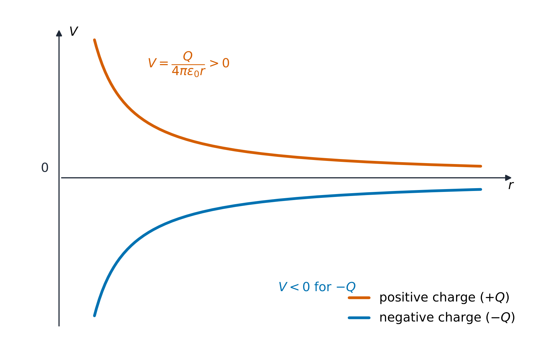
Electric potential 电势 is electric potential energy per unit charge at a point in space. It is measured in volts ($1\ \text{V}=1\ \text{J/C}$):
Potential is a scalar 标量: it has a sign but no direction. This makes $V$ far easier to work with than the field $\vec{E}$. For several point charges 点电荷, use scalar superposition 叠加 – add the potentials with their signs:
Worked example. The potential $0.10\ \text{m}$ from a $+3.0\ \text{nC}$ point charge is $V=\dfrac{kq}{r}=\dfrac{9.0\times10^{9}(3.0\times10^{-9})}{0.10}=270\ \text{V}$. Now add a $-3.0\ \text{nC}$ charge $0.30\ \text{m}$ from the same point: it contributes $\dfrac{9.0\times10^{9}(-3.0\times10^{-9})}{0.30}=-90\ \text{V}$, so the total is $270-90=180\ \text{V}$. Just a signed sum – no vector components to resolve.
Continuous charge distributions
For a continuous charge distribution 连续电荷分布, cut it into small pieces $dq$, treat each piece as a point charge, and integrate 积分:
This is a scalar integral, so it is usually much easier than the field integral. AP expects you to handle four shapes with calculus: a thin ring (at a point on its axis), an arc (at its centre), a finite line or wire (collinear, or on its perpendicular bisector), and an infinitely long wire or cylinder (at a distance from its axis).
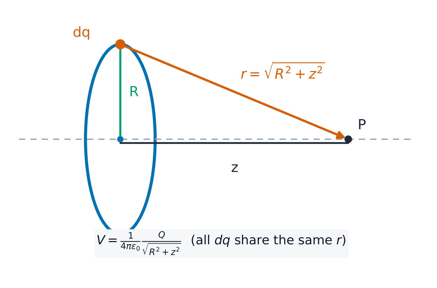
A ring of charge: every element dq is the same distance from an axis point
Worked example (ring of charge). A thin ring of radius $R$ carries total charge $Q$. For a point $P$ on the axis a distance $z$ from the centre, every element $dq$ sits at the same distance $r=\sqrt{R^2+z^2}$ from $P$. The distance is constant, so it comes out of the integral:
On an FRQ, say that $r$ is the same for every element – that statement is the marked step. The same idea gives $V=kQ/R$ at the centre of any arc, whatever its angle.
From potential to field
Potential and field contain the same information, linked by a derivative in each direction and by a path integral:
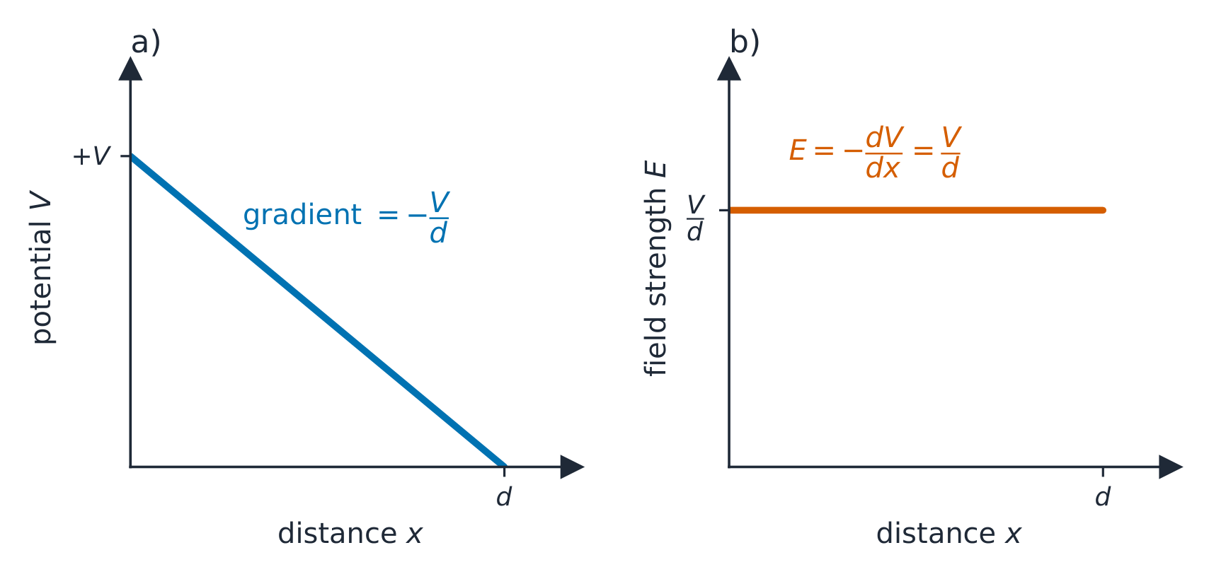
The field is the negative gradient 梯度 of the potential: $\vec{E}$ points from high potential to low potential, "downhill". Where $V$ changes quickly, the field is strong.
Worked example. Along the $x$-axis, $V(x)=3x^{2}-2x$ (volts, with $x$ in metres). Then $E_x=-\dfrac{dV}{dx}=2-6x\ \text{V/m}$. At $x=0.50\ \text{m}$, $E_x=-1.0\ \text{V/m}$: the field there points in the $-x$ direction.
In a uniform field the potential falls steadily with distance
The potential difference 电势差 between two points is the change in potential energy per unit charge moved between them: $\Delta V=\Delta U_E/q$. A battery makes a potential difference chemically: reactions inside separate positive from negative charge and hold the terminals a fixed $\Delta V$ apart.
The potential near a point charge varies as 1/r
Equipotential maps
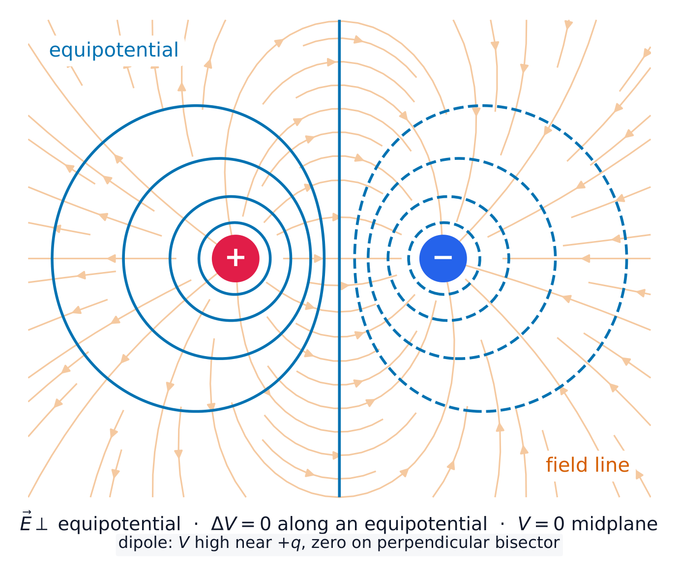
An equipotential 等势面 line (also called an isoline 等值线) joins points that share the same potential. Four rules let you read any map:
Isolines are perpendicular 垂直 to field lines 电场线 everywhere they cross.
$\vec{E}$ points from high $V$ to low $V$ – never along an isoline. Moving a charge along an isoline takes no work.
Closely spaced isolines mean a strong field: $E\approx-\Delta V/\Delta x$.
You can sketch the field map from an isoline map, and the isoline map from a field map.
Equipotential lines around a dipole cross the field lines at right angles
Exam skill. Given a map with isolines every $10\ \text{V}$ spaced about $2\ \text{cm}$ apart, estimate $E\approx\dfrac{10}{0.02}=500\ \text{V/m}$, pointing from the higher-value line to the lower one. The work an external agent does moving a charge $q$ slowly from $A$ to $B$ is $W=q(V_B-V_A)$ – the path taken does not matter.
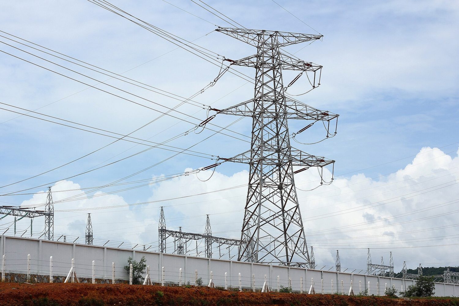
High-voltage power lines: electric potential energy is converted and transmitted as current at high voltage
탐색하기
전하 주위의 전기장 선과 전위
**전기 전위(electric potential)**는 단위 전하당 에너지입니다. 양전하로부터 거리가 멀어질수록 감소하며, 전기장 선은 높은 전위에서 낮은 전위로 향합니다.
학습 목표 9.3.A: 두 위치 사이의 전기포텐셜 차이로 인한 시스템의 변화를 설명하십시오.
9.3.A.1 충전된 물체가 서로 다른 전기포텐셜을 가진 두 위치 사이를 이동할 때, 물체-장 시스템의 전기포텐셜 에너지의 변화량은 다음 식으로 주어집니다.
식:$\Delta U_E = q\Delta V$
9.3.A.2 서로 다른 전기포텐셜을 가진 두 점 사이에서 충전된 물체가 이동하면 에너지 보존 법칙에 따라 물체의 운동 에너지가 변화합니다.
출처: College Board AP Course and Exam Description
When a charge $q$ moves between two points that differ in potential by $\Delta V$, the potential energy of the charge–field system changes by
$$\Delta U_E=q\,\Delta V.$$
If only the electric force acts, total energy is conserved, so the kinetic energy changes by the opposite amount:
$$\Delta K=-\Delta U_E=-q\,\Delta V.$$
Watch the two signs together: a positive charge speeds up when it moves to lower potential, while a negative charge speeds up when it moves to higher potential. Both are just the system trading potential energy for kinetic energy. This is how particle accelerators give charged particles their energy, and it underlies energy analysis in circuits.
Worked example. A proton ($q=1.6\times10^{-19}\ \text{C}$, $m=1.67\times10^{-27}\ \text{kg}$) starts at rest and is accelerated through a potential drop of $500\ \text{V}$ (it moves to lower potential, so $\Delta V=-500\ \text{V}$ and $\Delta K=-q\,\Delta V=+8.0\times10^{-17}\ \text{J}$). Setting $\Delta K=\tfrac12 mv^2$:
Exam skill. Choose energy methods, not kinematics, whenever the field is non-uniform or the path curves: only the end-point potentials matter. A typical FRQ chain is $q\,\Delta V \to \Delta K \to v$, with one line of justification: "the electric force is conservative, so energy is conserved."
9.3
Exam tips
Relate field and potential by $V=-\int \vec E\cdot d\vec l$ and $\vec E=-\nabla V$ (in 1-D, $E_x=-\tfrac{dV}{dx}$).
Potential is a scalar — add contributions with signs, no vector components needed.
Potential energy of a pair is $U=\tfrac{1}{4\pi\varepsilon_0}\tfrac{q_1 q_2}{r}$; use energy conservation for a charge's speed.
Know that no work is done moving along an equipotential, which is perpendicular to $\vec E$.
Choose the zero of potential (usually infinity) and state it.
10.1.A.2 도체가 정전기 평형 상태에 있을 때, 초과 전하 운반자 간의 상호 반발로 인해的这些运载体们完全位于导体表面。
10.1.A.2.i 순 음전하를 가진 도체에서 초과 전자는 도체 표면에 위치한다.
10.1.A.2.ii 순 양전하를 가진 도체에서 표면은 전자가 결핍되어 있으며, 이를 도체 표면에 양전하 운반자가 위치한다고 모델링할 수 있다.
10.1.A.3 초과 전하들은 도체 내부의 정전기 평형 상태를 형성하기 위해 도체 표면으로 이동한다.
10.1.A.3.i 도체 내부에서 전하가 정전기 평형에 도달하는 데 걸리는 시간 간격은 매우 짧아 무시할 수 있다.
10.1.A.3.ii 도체가 정전기 평형에 도달하면 도체 표면의 모든 점은 동일한 전기 퍼텐셜을 가지며, 도체는 등위면이 된다.
10.1.A.3.iii 도체 표면의 전하 밀도는 평평한 영역보다 점이나 모서리가 있는 부분에서 더 크다.
10.1.A.4 모든 잔여 전하는 도체 표면에 존재하므로 도체 내부에는 순전하가 없으며, 도체 내부의 전기장은 0이다.
10.1.A.5 전기장은 도체의 외부 표면과 수직이다.
10.1.A.6 도체는 외부 전기장 내에서 극화될 수 있다. 이는 도체가 등위면을 유지하기 때문的结果이다.
10.1.A.7 정전기 차폐는 특정 영역을 닫힌 도체 껍질로 둘러싸하여 도체 내부에 외부 전기장이 없는 영역을 생성하는 과정이다.
출처: College Board AP Course and Exam Description
In an ideal conductor 导体, electrons move freely. Put extra charge on one and the charges repel each other until, almost instantly, they settle into electrostatic equilibrium 静电平衡. In that state the conductor has four properties you must be able to state and use:
The electric field inside the conductor is zero. If it were not, free electrons would still be moving.
All excess charge sits on the surface. (Negative net charge = extra electrons on the surface; positive = a shortage of electrons there.)
The field just outside is perpendicular 垂直 to the surface, with magnitude $E=\sigma/\varepsilon_0$. Any parallel component would push charge sideways along the surface.
The whole conductor is one equipotential surface 等势面: every point, inside and on the surface, is at the same potential.
Charge density is largest where the surface curves sharply – at points and edges – so the outside field is strongest there. In an external field a conductor polarizes: charge shifts on its surface so that the interior stays field-free and the body stays an equipotential. Surrounding a region with a closed conducting shell keeps outside fields out entirely – electrostatic shielding 静电屏蔽, the idea behind the Faraday cage 法拉第笼.
학습 목표 10.2.A: 도체가 물리적으로 접촉할 때 전하의 이동과 이로 인한 상호작용을 설명한다.
10.2.A.1 도체가 전기적으로 접촉하면 각 도체 표면이 동일한 전기 퍼텐셜이 되도록 전하가 재분포된다.
10.2.A.2 접지(Ground)는 영(0)의 전기 퍼텐셜을 가진 이상화된 기준점이며, 전기 퍼텐셜을 변화시키지 않고 무한대의 전하를 흡수하거나 공급할 수 있다.
10.2.A.3 도체에 외부 전기장이 존재하는 상태에서 접지를 연결하면 도체에 전하가 유도될 수 있다.
출처: College Board AP Course and Exam Description
When two conductors touch (or are wired together), charge flows between them until both surfaces reach the same potential – that is the stopping condition, not "equal charges". A larger sphere holds more charge at the same potential ($V=kQ/R$), so it takes the larger share.
Worked example. A small sphere of radius $R$ carrying $+6.0\ \mu\text{C}$ touches a distant sphere of radius $2R$, then they separate. Equal potentials require $\dfrac{kq_1}{R}=\dfrac{kq_2}{2R}$, so $q_2=2q_1$. With $q_1+q_2=6.0\ \mu\text{C}$: $q_1=2.0\ \mu\text{C}$ and $q_2=4.0\ \mu\text{C}$.
Ground 接地 is an idealized reference at zero potential that can absorb or supply any amount of charge. Grounding a conductor while an external charge is nearby leaves the conductor with a net induced charge 感应电荷: the external field pushes charge of one sign to ground, and cutting the ground wire before removing the external charge traps the rest.
10.3.A.1 평판 콘덴서는 서로 분리된 두 개의 평행한 도체 면으로 구성되어 있으며, 서로 반대 부호의 동량의 전하를 저장할 수 있다.
10.3.A.2 정전용량은 각 판에 저장된 전하의 크기와 해당 전하들의 분리로 인해 생성된 전기 퍼텐셜 차이 사이의 관계를 나타낸다.
식:$C = \dfrac{Q}{\Delta V}$
10.3.A.2.i 콘덴서의 정전용량은 콘덴서의 형태 및 판 사이를隔开하는 데 사용된 재료와 같은 콘덴서의 물리적 특성에만 의존한다.
10.3.A.2.ii 평판 콘덴서의 정전용량은 한 판의 면적에 비례하고 판 사이의 거리에 반비례한다. 이 비례 상수는 판 사이의 재료의 유전 상수 $\kappa$와 진공의 전기유전율 $\varepsilon_0$의 곱이다.
식:$C = \dfrac{\kappa \varepsilon_0 A}{d}$
10.3.A.3 평판 콘덴서와 같이 전기 전하가 균일하게 분포된 두 개의 충전된 평행판 사이의 전기장은 판 가장자리 근처를 제외하고 크기와 방향 모두 일정하다.
10.3.A.3.i 판 간격이 판의 크기보다 훨씬 작은 두 개의 충전된 평행판 사이의 전기장 크기는 가우스 법칙과 중첩 원리를 적용하여 결정할 수 있다.
식:$E = \dfrac{Q}{\varepsilon_0 A}$
10.3.A.3.ii 전기장은 콘덴서 양쪽 판 중 하나의 표면 전하 밀도에 비례한다.
10.3.A.3.iii 서로 반대 부호로 충전된 두 평행판 사이에 있는 충전 입자는 일정한 가속도를 받으며, 따라서 질량을 가진 물체가 지구 표면 근처의 중력장에서 하는 투사체 운동과 유사한 특성을 가진다.
10.3.A.4 콘덴서에 저장된 전기 퍼텐셜 에너지는 그 양의 전하를 분리하기 위해 외부력이 한 일과 같다.
10.3.A.5 콘덴서에 저장된 전기 퍼텐셜 에너지는 식 $U_C = \dfrac{1}{2} Q \Delta V$로 기술된다.
경계 문구: 다른 형태도 전하를 분리할 수 있지만, AP Physics C: Electricity & Magnetism에서는 평판 콘덴서, 동심 구형 콘덴서, 동축 원통 콘덴서의 정량적 분석과 서술만 요구한다.
출처: College Board AP Course and Exam Description
Charging a capacitor (RC)
A capacitor 电容器 stores charge on two conductors separated by a gap: $+Q$ on one plate, $-Q$ on the other. Its capacitance 电容 relates the stored charge to the potential difference between the plates:
$$C=\frac{Q}{\Delta V}.$$
Capacitance depends only on geometry and the material in the gap – never on $Q$ or $\Delta V$ themselves.
Worked derivation (parallel plates). For a parallel-plate capacitor 平行板电容器 with plate area $A$ and small gap $d$: Gauss's law plus superposition 叠加 gives a uniform 均匀 field between the plates, $E=\dfrac{\sigma}{\varepsilon_0}=\dfrac{Q}{\varepsilon_0 A}$ (each plate alone contributes $\sigma/2\varepsilon_0$; between the plates the two add, outside they cancel). A uniform field means $\Delta V=Ed=\dfrac{Qd}{\varepsilon_0 A}$, so
This $E\to\Delta V\to C$ chain is a standard FRQ derivation – learn it as three steps, and quote each one. The same method handles the other two shapes AP expects: concentric spheres ($C=4\pi\varepsilon_0\dfrac{ab}{b-a}$) and a coaxial cylinder of length $L$, where $E=\dfrac{\lambda}{2\pi\varepsilon_0 r}$ gives $\Delta V=\dfrac{\lambda}{2\pi\varepsilon_0}\ln\dfrac{b}{a}$ and so $C=\dfrac{2\pi\varepsilon_0 L}{\ln(b/a)}$.
Worked example. Plates of area $A=0.020\ \text{m}^2$ and gap $d=1.0\ \text{mm}$: $C=\dfrac{8.85\times10^{-12}(0.020)}{1.0\times10^{-3}}=1.8\times10^{-10}\ \text{F}$. Charged to $100\ \text{V}$ it holds $Q=CV=1.8\times10^{-8}\ \text{C}$.
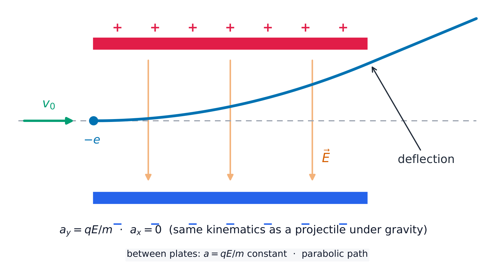
Because the field between the plates is uniform, a charged particle there feels a constant force, so it moves with constant acceleration – exactly like projectile motion 抛体运动 in gravity: constant speed across, uniform acceleration towards a plate.
A charged particle between the plates follows a parabola, like a projectile
Worked example. An electron enters midway between plates at $v_0=2.0\times10^{7}\ \text{m/s}$, parallel to them. The field is $E=1.0\times10^{3}\ \text{N/C}$ and the plates are $4.0\ \text{cm}$ long. Acceleration: $a=\dfrac{eE}{m}=\dfrac{(1.6\times10^{-19})(1.0\times10^{3})}{9.11\times10^{-31}}=1.8\times10^{14}\ \text{m/s}^2$. Time between the plates: $t=\dfrac{0.040}{2.0\times10^{7}}=2.0\times10^{-9}\ \text{s}$. Deflection: $y=\tfrac12at^{2}=\tfrac12(1.8\times10^{14})(2.0\times10^{-9})^{2}\approx3.5\times10^{-4}\ \text{m}$ – about $0.35\ \text{mm}$ towards the positive plate.
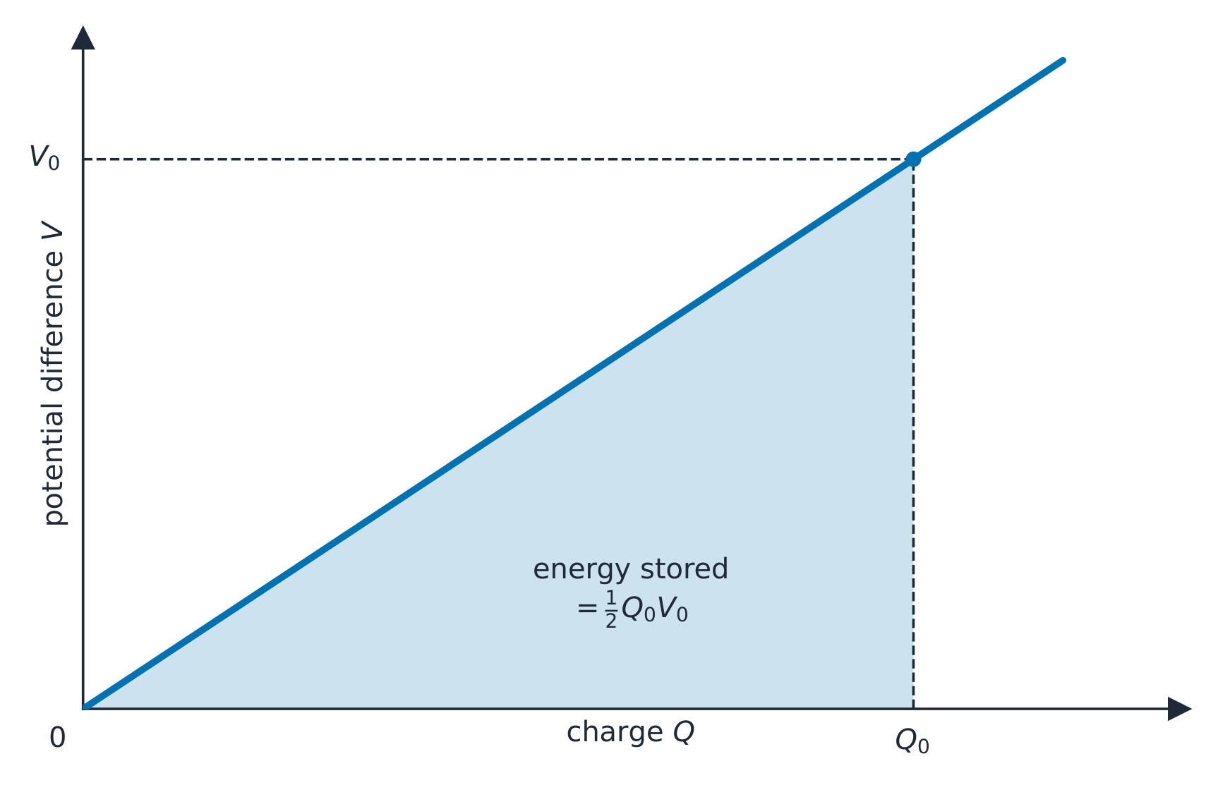
Storing charge takes work 功: an external force must move each bit of charge against the field of the charge already there. The total work ends up as stored potential energy,
The energy stored in a capacitor is the area under its charge-voltage line
The factor $\tfrac12$ is the area of the triangle under the $Q$–$\Delta V$ line: the first charge moved across costs almost nothing, the last costs the full $\Delta V$.
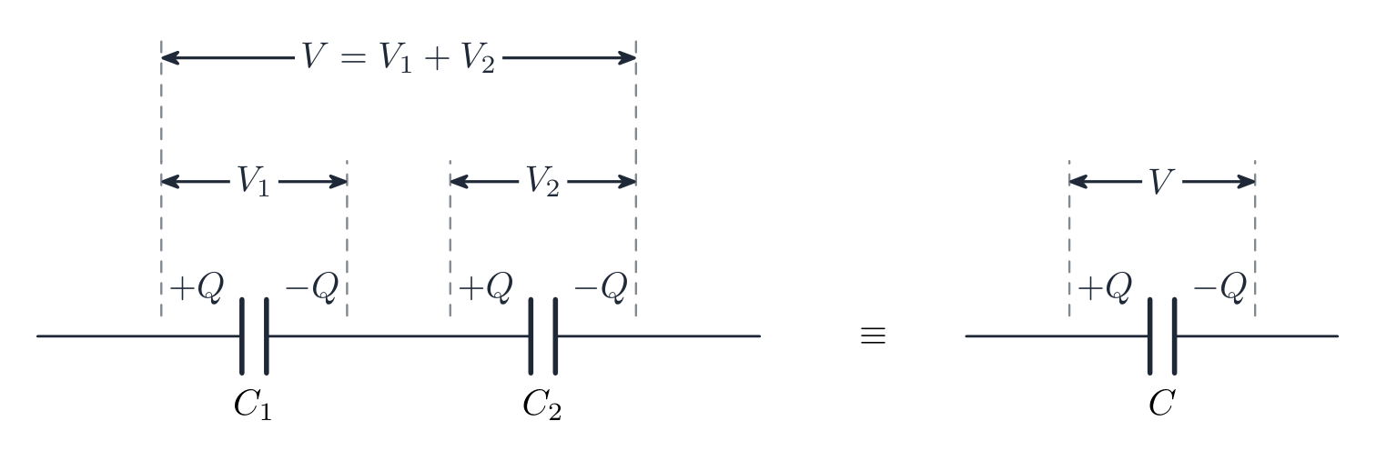
Capacitors combine oppositely to resistors: in parallel 并联 the capacitances add ($C_{\text{eq}}=C_1+C_2$, same $\Delta V$, charges add), while in series 串联 the reciprocals add ($\tfrac{1}{C_{\text{eq}}}=\tfrac{1}{C_1}+\tfrac{1}{C_2}$, same $Q$, voltages add).
Capacitors in series carry the same charge, and their p.d.s add
Worked example. A $2\ \mu\text{F}$ and a $4\ \mu\text{F}$ capacitor in series: $\tfrac{1}{C}=\tfrac12+\tfrac14$, so $C=\tfrac43\ \mu\text{F}$. The same pair in parallel: $6\ \mu\text{F}$.
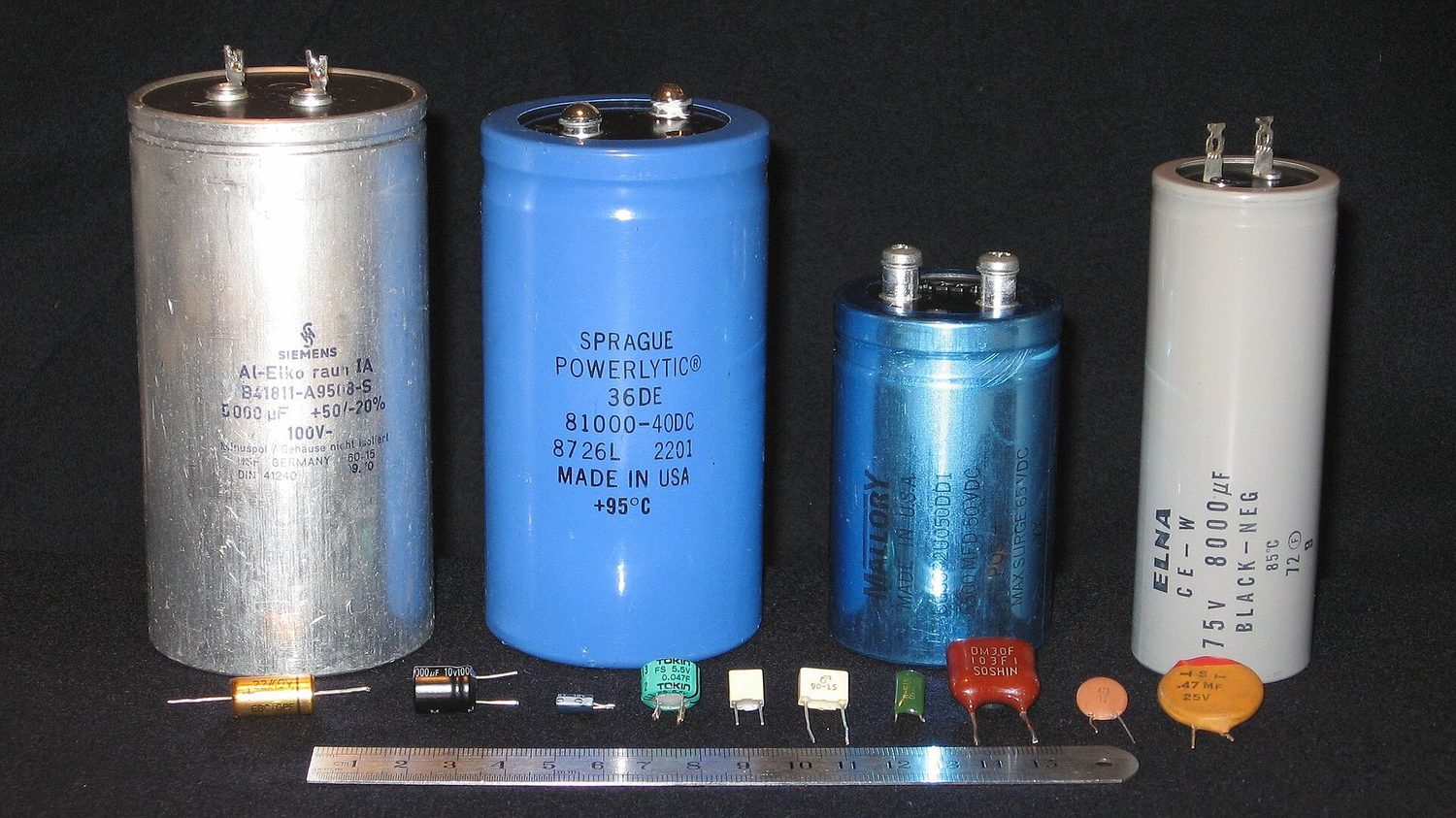
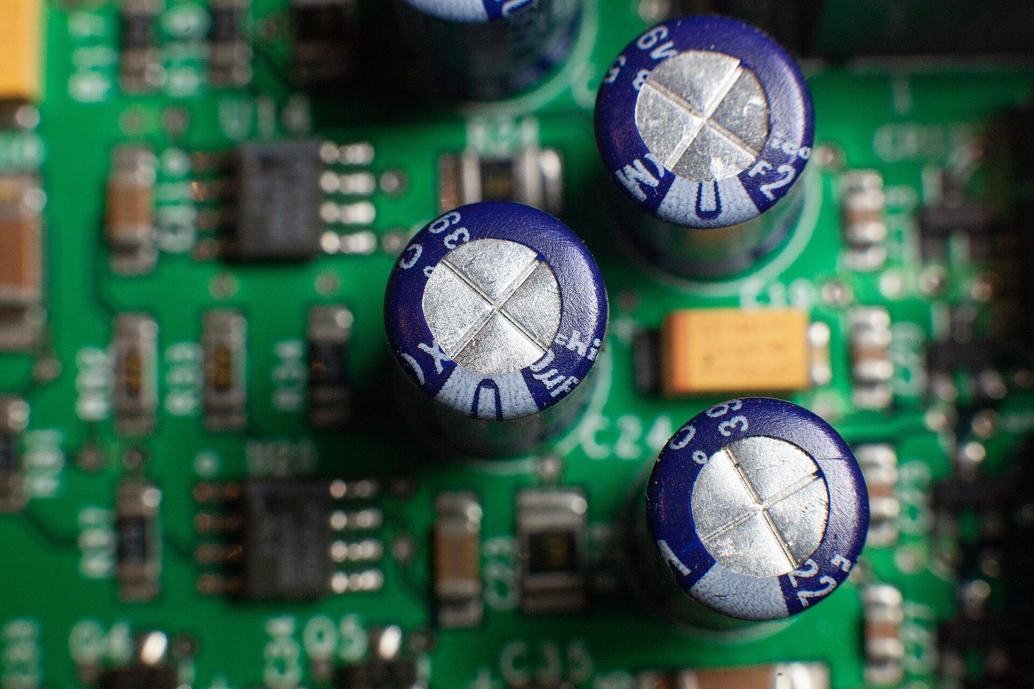
Assorted capacitors: devices that store charge and energy in an electric field between conductorsElectrolytic capacitors on a circuit board: capacitance stores energy as U = ½CV²
탐색하기
콘덴서를 충전하고 방전하기
**축전기(capacitor)**는 두 극판에 전하를 저장하며, 시간 상수 $\tau=RC$에 따라 지수함수적으로 충전되고 방전됩니다. $R$나 $C$가 클수록 충전/방전 속도가 느려집니다.
학습 목표 10.4.A: 콘덴서 판 사이에 유전체를 삽입하면 콘덴서의 성질이 어떻게 변하는지 설명한다.
10.4.A.1 유전체 소재 내에서는 도체처럼 전하가 자유롭게 움직이지 못한다. 대신 외부 전기장이 존재할 때 소재가 극화된다.
10.4.A.2 유전 상수는 해당 소재의 전기유전율을 진공의 전기유전율과 연결시킨다.
식:$\kappa = \dfrac{\varepsilon}{\varepsilon_0}$
10.4.A.3 극화된 유전체가 생성하는 전기장은 외부 전기장의 방향과 반대이다.
10.4.A.4 고립된 평판 콘덴서 판 사이에 유전체를 넣으면 판 사이의 전기장이 감소한다.
식:$\kappa = \dfrac{E_0}{E}$
10.4.A.5 콘덴서에 유전체를 삽입하면 콘덴서의 정전용량이 변할 수 있다.
식:$C = \kappa C_0$
출처: College Board AP Course and Exam Description
A dielectric 电介质 is an insulating material. Its charges cannot travel, but in an external field each molecule stretches or turns slightly – the material becomes polarized 极化. The lined-up molecules create their own small field opposite to the applied one, so the net field inside the material drops:
What happens next depends on what stays fixed – a favourite exam trap:
battery stays connected ($\Delta V$ fixed)
battery removed first ($Q$ fixed)
charge $Q$
rises to $\kappa Q_0$
unchanged
voltage $\Delta V$
unchanged
drops to $\Delta V_0/\kappa$
field $E$
unchanged
drops to $E_0/\kappa$
energy $U$
rises to $\kappa U_0$
drops to $U_0/\kappa$
Worked example. A $100\ \text{pF}$ capacitor is charged to $12\ \text{V}$, disconnected, then filled with a $\kappa=3$ dielectric. $Q$ is trapped, so $\Delta V$ falls to $4\ \text{V}$ and the stored energy falls to one-third – the missing energy went into pulling the dielectric in. Reconnected to the $12\ \text{V}$ battery instead, the capacitor would hold three times the charge and three times the energy.
Exam skill. Always begin dielectric questions by writing down which quantity is held fixed ($Q$ or $\Delta V$), then let $C=\kappa C_0$ drive everything else through $Q=C\Delta V$ and $U=\tfrac12 C(\Delta V)^2$.
탐색하기
유전체 추가
극판 사이의 **유전체(dielectric)**는 정전 용량을 증가시켜 동일한 전압에서 더 많은 전하를 저장할 수 있게 합니다. 전하가 더 빠르게 쌓이는 것을 보세요.
11.1.A.4 전류는 스칼라량이지만 방향을 가진다. 그러나 그 방향은 공간이 아닌 전하 운반자와의 상대성이므로, 전류는 벡터 덧셈 법칙을 따르지 않으며 벡터 성분을 가지지 않는다.
11.1.A.4.i conventional current(정전류)의 방향은 양전하가 이동할 것으로 가정되는 방향으로 설정된다.
11.1.A.4.ii 일반적인 회로에서 실제 전류는 전자(음전하 운반자)의 이동에 의해 발생한다.
출처: College Board AP Course and Exam Description
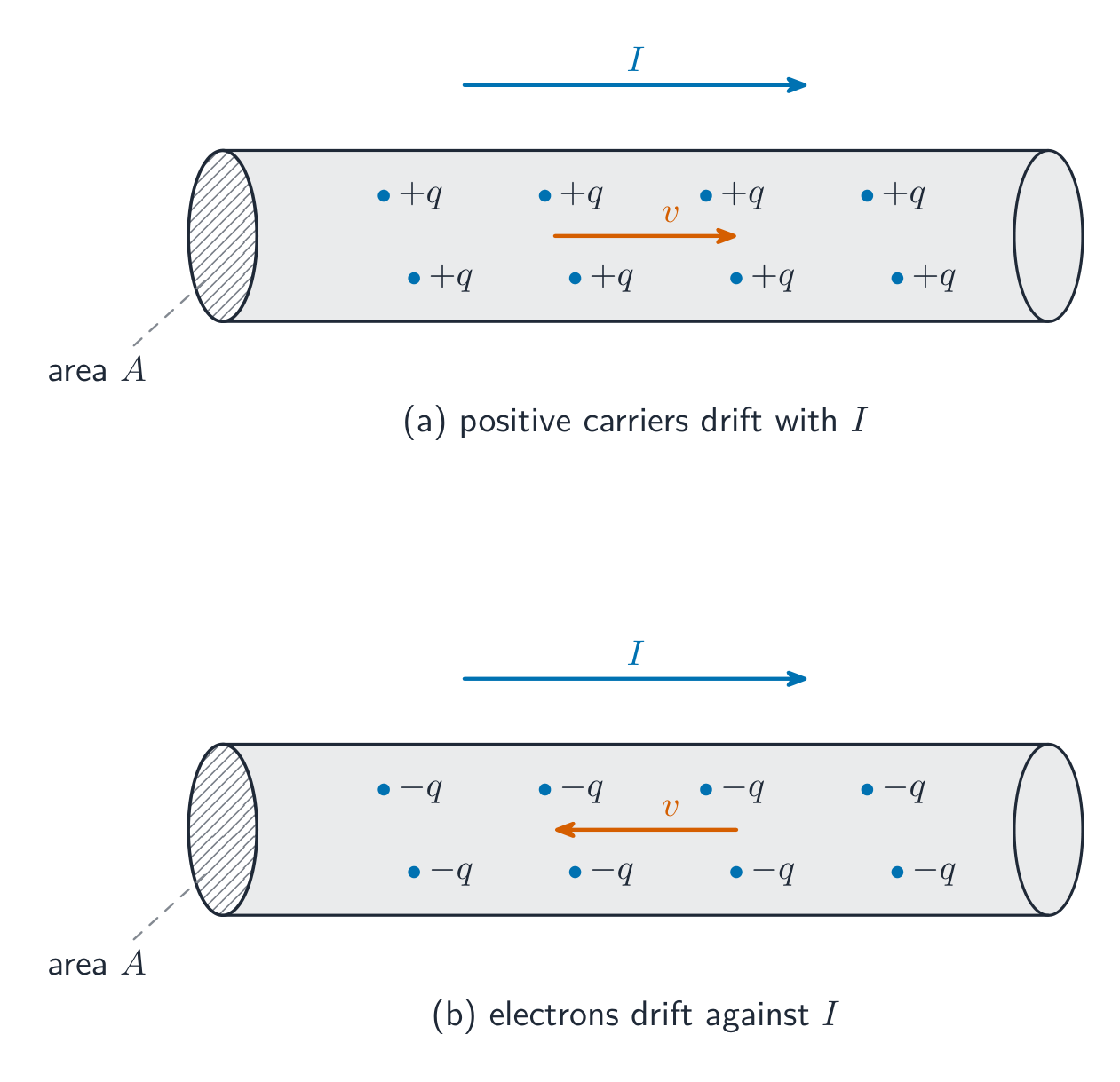
전기 전류는 단면적을 통과하는 전하의 흐름률, $I=\dfrac{dq}{dt}$이며, 암페어(A) 단위로 측정됩니다. 관례적 전류는 양전하가 이동할 방향을 가리킵니다. 미시적으로는 전류는 수많은 운반자가 느리게 흐르는 drift 현상입니다:
$$I=nqv_dA,$$
여기서 $n$는 단위 부피당 운반자의 수, $q$은 각 운반자가 가진 전하량, $v_d$는 드리프트 속도, $A$은 단면적입니다.
전하 운반체는 전류를 만들기 위해 도체를 통해 느리게 흐립니다
풀이 예제. 단면적 $A=1.0\times10^{-6}\ \text{m}^2$와 전하 밀도 $n=8.5\times10^{28}\ \text{m}^{-3}$을 가진 구리 도선에 전류 $1.7\ \text{A}$가 흐릅니다. 그러면 드리프트 속도는 $v_d=\dfrac{I}{nqA}=\dfrac{1.7}{(8.5\times10^{28})(1.6\times10^{-19})(1.0\times10^{-6})}\approx1.3\times10^{-4}\ \text{m/s}$입니다 – 신호가 빛의 속도에 가깝게 전달되더라도 운반자의 드리프트 속도는 달보다 느립니다.
전류밀도는 단위 면적당 흐르는 전하량, 즉 $\vec{J}=nq\vec{v}_d$이며, 이를 유도하는 장과의 관계는 $\vec{E}=\rho\vec{J}$로 주어집니다. 일반적으로 $I=\int\vec{J}\cdot d\vec{A}$입니다. 만약 $J(r)$가 도선의 단면에서 불균일하게 분포한다면, 총전류를 구하기 위해 단면 전체에 대해 적분해야 합니다. 주의할 점은: 전류는 도선을 따라 방향을 가지지만 스칼라 quantity입니다. 따라서 전류는 벡터처럼 더하지 않으며, '전류의 성분'이라는 개념은 존재하지 않습니다.
11.2.A.1 회로는 wires, 배터리, 저항기, 전구, 콘덴서, 인덕터, 스위치, 아머미터, 볼트미터 등을 포함할 수 있는 전기 루프로 구성된다.
11.2.A.2 폐회로( rumors circuit )는 전하가 흐를 수 있는 닫힌 경로이다.
11.2.A.2.i 폐회로는 전하가 흐를 수 있는 회로이다.
11.2.A.2.ii 개회로는 전하가 흐를 수 없는 회로이다.
11.2.A.2.iii 단락 회로는 전하가 전위차 변화 없이 흐를 수 있는 회로이다.
11.2.A.3 하나의 회로 요소가 여러 전기 루프의 일부가 될 수 있다.
11.2.A.4 회로도(schematic diagram)는 전기 회로를 서술하고 분석하기 위해 사용되는 표현법이다.
11.2.A.4.i 전기회로의 특성은 constituent 요소들의 물리적 배치에 의존한다.
11.2.A.4.ii 회로 요소에는 회로도를 그릴 때 사용되는 표준 기호가 있다. 가변 요소는 해당 요소의 표준 기호 위에 대각선으로 뚫린 화살표로 표시한다. (기호: 배터리, 전구, 스위치, 콘덴서, 저항기, 아머미터, 볼트미터, 인덕터.)
경계 명제: 별도 명시하지 않는 한 모든 회로도 그림은 통상 전류를 사용하여 그려진다.
출처: College Board AP Course and Exam Description
회로는 전선, 배터리, 저항기, 전구, 콘덴서, 인덕터, 스위치 및 계측기 등으로 구성된 폐쇄 루프의 집합입니다. 전하는 오직 폐쇄된 경로를 따라 흐를 수 있습니다. 하나의 요소가 여러 루프에 동시에 속할 수 있는데, 이것이 다중 루프 문제의 흥미로운 지점입니다. 모든 분석은 회로도를 읽는 것부터 시작됩니다. 각 루프를 따라가며 어떤 요소들이 같은 전류를 공유하는지(직렬) 또는 같은 전위차를 공유하는지(병렬)를 식별하십시오.
탐색하기
직렬 및 병렬 회로 만들기
직렬 회로에서는 모든 전구를 통해 동일한 전류가 흐르고 전압이 분배됩니다. 병렬 회로에서는 각 가지에 전체 전압이 인가됩니다. 스위치 모드를 사용하여 전구의 밝기 변화를 확인하세요.
11.3
저항, 저항율, 그리고 옴의 법칙
Syllabus
학습 목표 11.3.A: 물체의 물리적 성질을 사용하여 그 물체의 저항을 설명하시오.
11.3.A.1 저항은 물체가 전기전하의 이동을 얼마나 저해하는지를 나타내는 척도이다.
11.3.A.2 균일한 기하학적 형상을 가진 저항기의 저항은 그 저항율과 길이에 비례하며, 단면적에 반비례한다.
식:$R = \dfrac{\rho\ell}{A}$
11.3.A.2.i 저항율은 물질의 원자 및 분자 구조에 의존하는 물질의 근본적 성질로서, 물질이 전기전하의 운동을 얼마나 강하게 저해하는지를 정량화한다.
11.3.A.2.ii 도체의 저항율은 일반적으로 온도가 올라갈수록 증가한다.
11.3.A.2.iii 균일한 형상을 갖지만 저항길이에 따라 저항률이 변하는 소재로 만들어진 저항기의 총 저항은 $R = \int \dfrac{\rho(\ell)\,d\ell}{A}$로 주어진다.
학습 목표 11.3.B: 회로 요소의 전기적 특성을 설명하시오.
11.3.B.1 옴의 법칙은 회로의 전도성 요소에 흐르는 전류, 저항, 그리고 전위차 사이의 관계를 나타낸다.
식:$I = \dfrac{\Delta V}{R}$
11.3.B.1.i 옴의 법칙을 따르는 물질은 모든 전류에 대해 일정한 저항을 가지며 이를 옴 물질(Ohmic material)이라 한다.
11.3.B.1.ii 옴 물질의 저항율은 온도에 관계없이 일정하다.
11.3.B.1.iii 저항기는 또한 전기 에너지를 열에너지로 변환할 수 있으며, 이는 저항기 자체와 주변 환경의 온도 변화를 초래할 수 있다.
11.3.B.1.iv 옴 회로 요소의 저항은 해당 요소에 걸린 전위차에 대한 요소 내 전류의 그래프 기울기로부터 결정할 수 있다.
출처: College Board AP Course and Exam Description
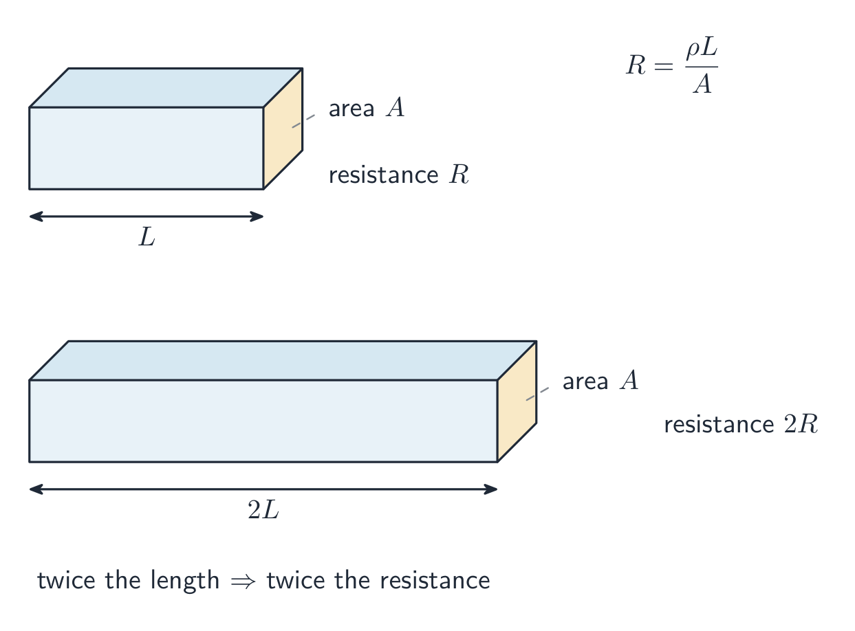
저항은 물체가 전하 흐름을 얼마나 강하게 방해하는지를 측정합니다. 그것은 소재의 저항률과 도체의 길이에 비례하여 증가하고, 단면적에 반비례하여 감소합니다:
$$R=\frac{\rho\,\ell}{A}.$$
옴의 법칙은 요소를 통과하는 전류와 그 양단에 걸리는 전위차 사이의 관계를 나타냅니다:
$$I=\frac{\Delta V}{R}.$$
더 긴 도체는 더 큰 저항을 가지며, 더 넓은 도체는 더 작은 저항을 가집니다
worked example. 선을 늘려 길이를 두 배로 만드십시오: 부피가 일정하므로 단면적이 절반이 되며, $R=\rho\ell/A$는 $\rho(2\ell)/(A/2)=4R$이 되어 – 저항은 네 배가 됩니다. ⟨$R$⟩이 일정하면(원점을 지나는 직선인 $I$–$\Delta V$ 그래프상에서) 해당 요소는 옴 소자(ohmic) 이라고 합니다. 열이 발생하는 전구 필라멘트는 옴 소자가 아닙니다.
탐색하기
옴의 법칙 적용하기
옴의 법칙$V=IR$: 저항이 일정할 때 전류는 전압에 비례합니다. 저항을 높이면 동일한 전압에서도 흐르는 전류는 줄어듭니다.
학습 목표 11.4.A: power를 사용하여 전기회로로 들어가는, 나가는, 혹은 내부에서의 에너지 전달을 설명하시오.
11.4.A.1 회로 요소에 의해 전달, 변환, 또는 소모되는 에너지의 속도는 해당 요소의 전류와 요소에 걸린 전기적 전위차에 의존한다.
식:$P = I\Delta V$
식:$P = I^2 R = \dfrac{\Delta V^2}{R}$
11.4.A.2 전구의 밝기는 출력(power)에 비례하여 증가하므로, 출력은 회로 내 전구의 밝기를 질적으로 예측하는 데 사용할 수 있다.
경계문: AP Physics C: Electricity & Magnetism에서는 학생들에게 기계 에너지와 전기 에너지의 전달만 분석하도록 요구하지만, 학생들은 전기 에너지가 열에너지 형태로 소산될 수도 있다는 점을 인지하고 있어야 한다.
출처: College Board AP Course and Exam Description
전하 $q$가 전위차 $\Delta V$를 통과할 때 에너지 $q\Delta V$를 방출하므로, 요소에서의 에너지 전달율은 다음과 같습니다:
$$P=I\,\Delta V=I^2R=\frac{(\Delta V)^2}{R}.$$
저항기에서는 모든 에너지가 열로 변합니다. 실제로 알고 있는 양을 가진 식을 사용하십시오 – 그리고 전구의 밝기를 비교하기 위해 전력(power) 을 사용하십시오: 더 밝다 = 더 많은 전력, 반드시 더 큰 저항을 의미하지는 않습니다. 직렬에서는 크기가 큰 저항기가 더 밝습니다 ($P=I^2R$, 동일한 $I$); 병렬에서는 크기가 작은 것이 더 밝습니다 ($P=\Delta V^2/R$, 동일한 $\Delta V$).
탐색하기
I-V 특성 곡선 읽기
전력은 $P=IV$입니다. 저항기의 I-V 선은 직선이지만, 전구는 발열하며 저항이 증가함에 따라 곡선을 그립니다. I-V 곡선 아래 면적은 전달된 에너지와 관련이 있습니다.
11.5
복합 직류 회로
Syllabus
학습 목표 11.5.A: 회로에 연결된 여러 저항기의 등가 저항을 설명하시오.
11.5.A.1 회로 요소는 직렬 및/또는 병렬로 연결될 수 있다.
11.5.A.1.i 직렬 연결은 하나의 회로 요소를 통과한 전하가 반드시 해당 연결의 모든 요소를 지나야 하며 다른 경로를 사용할 수 없는 경우이다. 직렬로 연결된 각 요소의 전류는 동일해야 한다.
11.5.A.1.ii 병렬 연결은 전하가 두 개 이상의 경로 중 하나를 통과할 수 있는 연결 방식이다. 각 경로 간에는 전위차가 동일하다.
11.5.A.2 회로 내 저항기의 집합은 등가 저항 $R_{\text{eq}}$을 가진 단일 저항기로 처리하여 분석할 수 있습니다.
11.5.A.2.i 직렬로 연결된 저항기 집합의 등가 저항은 개별 저항들의 합과 같습니다.
식:$R_{\text{eq},s} = \sum_{i} R_i$
11.5.A.2.ii 병렬로 연결된 저항기 집합의 등가 저항의 역수는 개별 저항들의 역수의 합과 같습니다.
11.5.A.2.iii 저항기를 병렬로 연결하면 전하가 흐를 수 있는 경로 수가 증가하고, 저항기 집합의 등가 저항은 감소합니다.
학습 목표 11.5.B: 저항성 도선과 내부 저항이 있는 배터리가 포함된 회로를 설명하십시오.
11.5.B.1 이상적인 배터리는 내부 저항이 무시할 수 있을 정도로 작습니다. 이상적인 도선은 저항이 무시할 수 있을 정도로 작습니다.
11.5.B.1.i 좋은 도체인 도선의 저항은 일반적으로 회로의 다른 요소에 비해 훨씬 작으므로 무시할 수 있습니다.
11.5.B.1.ii 회로에 저항이 있는 다른 요소가 포함되어 있을 때만 도선의 저항을 무시할 수 있습니다.
11.5.B.1.iii 배터리가 이상적일 경우 공급할 전위차는 배터리에 전류가 흐르지 않을 때 단자 간에 측정되는 전위차이며, 이를 때때로 $\mathrm{emf}$($\mathcal{E}$)이라고 부릅니다.
11.5.B.2 비이상적인 배터리의 내부 저항은 이상적인 배터리와 회로의 나머지 부분에 직렬로 연결된 저항기의 저항으로 간주할 수 있습니다.
11.5.B.3 내부 저항 $r$이 있는 비이상적인 배터리에 전류가 흐를 때, 배터리의 단자 간 전위차는 배터리에 전류가 흐르지 않을 때의 전위차보다 낮아집니다.
식:$\Delta V_{\text{terminal}} = \mathcal{E} - Ir$
학습 목표 11.5.C: 회로 내 전류 및 전위차의 측정 방법을 설명하십시오.
11.5.C.1 아메트르는 회로의 특정 지점에서의 전류를 측정하는 데 사용됩니다.
11.5.C.1.i 아메트는 전류를 측정하려는 요소와 직렬로 연결되어야 합니다.
11.5.C.1.ii 이상적인 아메트는 직렬로 연결된 요소의 전류에 영향을 주지 않도록 저항이 0이어야 합니다.
11.5.C.2 볼트미터는 회로의 두 점 사이의 전기 전위차를 측정하는 데 사용됩니다.
11.5.C.2.i 볼트미터는 전위차를 측정하려는 요소와 병렬로 연결되어야 합니다.
11.5.C.2.ii 이상적인 볼트미터는 무한대의 저항을 가지므로 이를 통과하는 전하 흐름이 없다.
11.5.C.3 비이상적인 아메트와 볼트미터는 측정 대상 회로의 특성을 변경할 수 있습니다.
*경계문:*特别的히 명시하지 않는 한, 모든 배터리, 선, 그리고 계측기(meters)는 이상적이라고 가정한다. 서로 다른 전위차를 가진 배터리를 병렬로 연결한 회로는 평가 대상이 아니다.
출처: College Board AP Course and Exam Description
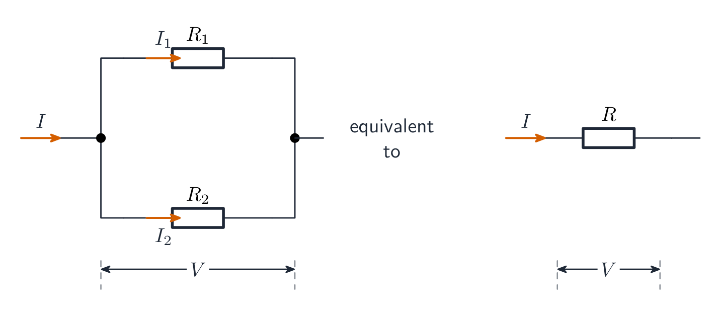
저항 네트워크를 등가 저항(equivalent resistance) 으로 축소하십시오: 직렬 저항기는 더합니다 ($R_{\text{eq}}=R_1+R_2+\cdots$), 병렬 저항기는 역수 합으로 계산됩니다 ($\tfrac{1}{R_{\text{eq}}}=\tfrac{1}{R_1}+\tfrac{1}{R_2}+\cdots$ – 항상 가장 작은 분지보다 작습니다). 스텝-by-step으로 네트워크를 축소하여 배터리 전류를 구한 후, 다시 확장하여 각 요소의 전류와 전압을 찾으십시오.
실제 배터리는 이상적인 배터리가 아닙니다. EMF $\varepsilon$인 이상 배터리와 자체 내부 저항$r$이 직렬로 연결된 모델로 배터리를 표현하십시오. 전류가 흐르면 내부에서 일부 EMF가 소모되므로, 단자 전압(terminal voltage) – 배터리에 병렬로 연결된 전압계가 실제로 읽는 값 – 은 감소합니다:
$$\Delta V_{\text{terminal}}=\varepsilon-Ir.$$
Worked example. EMF $\varepsilon=12\ \text{V}$와 내부 저항 $r=0.50\ \Omega$을 가진 배터리가 전류 $2.0\ \text{A}$를 공급할 때, 단자 전위는 $\Delta V=12-2.0(0.50)=11\ \text{V}$입니다. 전류가 없을 때 전압계는 전체 EMF $12\ \text{V}$를 읽습니다.
계측기: 아머미터(ammeter) 는 원하는 전류의 지점에 직렬로 연결합니다 (이상 아머미터: 제로 저항); 볼트미터(voltmeter) 는 요소 양단에 병렬로 연결합니다 (이상 볼트미터: 무한대 저항). 비이상 계측기는 측정하는 회로를 교란시킵니다 – 실제 아머미터는 직렬 저항을 추가하고, 실제 볼트미터는 회로에서 전류를 빼앗습니다.
학습 목표 11.6.A: 키르히호프의 루프 법칙을 적용하여 회로 또는 회로의 요소를 설명하십시오.
11.6.A.1 단순 전기 회로의 에너지 변화는 회로 요소 내의 전기 전위차를 통해 이동하는 전하의 관점으로 표현될 수 있습니다.
식:$\Delta U_E = q\Delta V$
11.6.A.2 키르히호프의 루프 법칙은 에너지 보존 법칙의 결과입니다.
11.6.A.2.i 키르히호프의 루프 법칙에 따르면 단일 폐루프 내의 모든 회로 요소를 통과한 전위차의 합은 0이어야 한다.
식:$\sum \Delta V = 0$
11.6.A.2.ii 회로의 특정 지점에서의 전기 전위 값은 루프 내 위치 함수로서의 전기 전위를 나타내는 그래프로 표현할 수 있다.
출처: College Board AP Course and Exam Description
전하가 전위차를 이동하며 에너지를 교환합니다 ($\Delta U_E=q\Delta V$), 그리고 에너지는 임의의 폐쇄된 경로에서 균형을 이루어야 합니다. 이것이 키르히호프의 루프 규칙(Kirchhoff's loop rule) 입니다:
$$\sum\Delta V=0\ \text{around any closed loop}.$$
부호 규율(sign discipline)은 이 문제를 해결하는 열쇠입니다: 배터리에서 $-$에서 $+$로 Crossing 할 때는 $+\varepsilon$; 저항기를 가정한 전류 방향과 같이 Crossing 할 때는 $-IR$ (반대로 Crossing 할 때는 $+IR$). 독립 루프마다 하나의 식을 쓰십시오.
학습 목표 11.7.A: 키르히호프의 접점 법칙을 적용하여 회로 또는 회로의 요소를 설명하십시오.
11.7.A.1 키르히호프의 접점 법칙은 전기电荷 보존 법칙의 결과입니다.
11.7.A.2 키르히호프의 접점 법칙은 단위 시간당 접점에 유입되는 총 전하량이 해당 접점에서 유출되는 총 전하량과 같아야 한다고 명시합니다.
식:$\sum I_{\text{in}} = \sum I_{\text{out}}$
출처: College Board AP Course and Exam Description
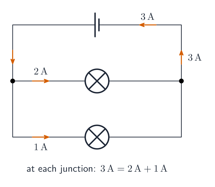
키르히호프의 접점 규칙(Kirchhoff's junction rule) 은 접점(junction) 에서의 전하 보존입니다:
$$\sum I_{\text{in}}=\sum I_{\text{out}}.$$
접점에서 전류가 분할됨: 유입된 것은 유출된 것과 같음
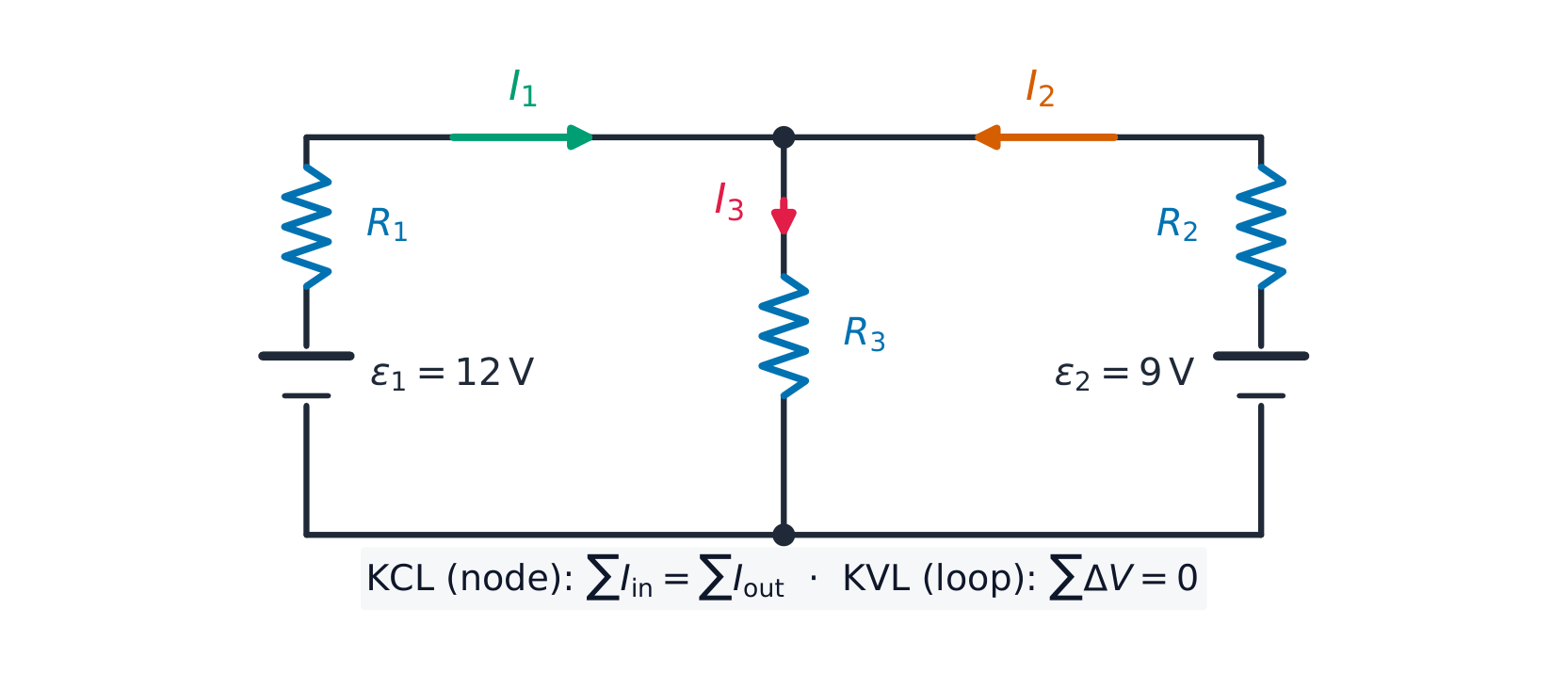
두 규칙을 함께 사용하면 모든 다중 루프 회로를 풀 수 있습니다: 각 분지에 전류를 할당하고, 접점 식을 쓴 다음 루프 식을 써서 풀십시오. 음수 답은 단순히 전류가 가정한 방향과 반대 방향으로 흐른다는 것을 의미합니다.
두 개의 루프 식과 하나의 접점 식이 이 두 배터리 회로를 풉니다
Worked example. 위 회로에서, 왼쪽에 $\varepsilon_1=12\ \text{V}$와 $R_1=1.0\ \Omega$이 있고, 오른쪽에 $\varepsilon_2=9.0\ \text{V}$와 $R_2=1.0\ \Omega$이 있으며, 공유되는 중간 저항기 $R_3=2.0\ \Omega$에는 $I_3=I_1+I_2$이 흐릅니다 (접점 규칙). 두 루프 식은 다음과 같습니다:
11.8.A.1.ii 직렬로 연결된 콘덴서 집합의 등가 정전용량은 가장 작은 콘덴서의 정전용량보다 작습니다.
11.8.A.1.iii 병렬로 연결된 콘덴서 집합의 등가 정전용량은 개별 정전용량의 합과 같습니다.
식:$C_{\text{eq},p} = \sum_{i} C_i$
11.8.A.2电荷守恒의 결과, 직렬로 연결된 각 콘덴서의 각 극판에는 동일한 크기의 전하가 존재해야 합니다.
학습 목표 11.8.B: 저항기와 콘덴서의 조합이 포함된 회로의 거동을 설명하십시오.
11.8.B.1 RC 회로 내 콘덴서의 전하 또는 저항기의 전류는 키르히호프의 루프 규칙으로부터 유도된 기본 미분 방정식으로 기술할 수 있다.
식:$\mathcal{E} = \dfrac{dq}{dt}R + \dfrac{q}{C}$
11.8.B.2 시간 상수(time constant, $\tau$)는 RC 회로의 중요한 특징이다.
11.8.B.2.i RC 회로의 시간 상수는 콘덴서가 충전하거나 방전되는 속도를 나타내는 지표이며, $\tau = R_{\text{eq}}C_{\text{eq}}$로 정의된다.
11.8.B.2.ii 충전 중인 콘덴서의 경우, 시간 상수는 콘덴서의 전하량이 0에서 최종 점근값의 약 63%까지 증가하는 데 걸리는 시간을 의미한다.
11.8.B.2.iii 방전 중인 콘덴서의 경우, 시간 상수는 콘덴서의 전하량이 완전 충전 상태에서 초기값의 약 37%까지 감소하는 데 걸리는 시간을 의미한다.
11.8.B.3 콘덴서에 걸린 전위차와 콘덴서를 포함하는 회로 분기의 전류는 콘덴서가 충전 및 방전됨에 따라 시간에 따라 변하지만, 긴 시간 간격 후 모두 정상 상태(steady state)에 도달하게 된다.
11.8.B.3.i 회로에 바로 연결되었을 때 미충전 콘덴서는 전선과 같이 동작하여 콘덴서 판에 전하가 쉽게 흐를 수 있다.
11.8.B.3.ii 콘덴서가 충전됨에 따라 콘덴서 양단간의 전위차 변화는 콘덴서 판에 축적된 전하량, 콘덴서가 위치한 회로의 가지에 흐르는 전류, 그리고 콘덴서에 저장된 전기ポテン셜 에너지에 영향을 미친다.
11.8.B.3.iii 콘덴서 양단 전압, 콘덴서가 위치한 회로 분지의 전류, 그리고 콘덴서에 저장된 전기 포텐셜 에너지는 모두 시간에 따라 변화하며 점진적으로 정태 상태(steady state)에 수렴한다.
11.8.B.3.iv 충분히 긴 시간이 지난 후, 충전 중인 콘덴서는 완전 충전된 상태에 근접하며, 이때 콘덴서가 위치한 회로 분지에는 전류가 흐르지 않고 최대 전압이 도달한다.
11.8.B.3.v 충전된 콘덴서가 방전을 시작하는 즉시, 콘덴서의 전하량과 콘덴서에 저장된 에너지는 감소하기 시작한다.
11.8.B.3.vi 콘덴서가 방전됨에 따라 콘덴서의 전하량, 콘덴서 양단간의 전위차, 그리고 콘덴서가 위치한 회로의 가지에 흐르는 전류는 모두 안정 상태(steady state)에 도달할 때까지 감소한다.
11.8.B.3.vii 충전 또는 방전이 시간 상수(time constant)보다 훨씬 긴 시간이 경과한 후에는, 콘덴서와 관련 회로 분지를 정태 조건을 사용하여 모델링할 수 있다.
출처: College Board AP Course and Exam Description
축전기 방전: τ = RC콘덴서 충전(RC)
콘덴서 네트워크도 저항기와 마찬가지로 축소되지만 규칙이 바뀝니다: 병렬 콘덴서는 더합니다 ($C_{\text{eq}}=C_1+C_2$), 직렬은 역수 합으로 계산됩니다 – 그리고 전하 보존에 의해 직렬 콘덴서는 각 극판에 같은 전하를 가져야 합니다. 등가 콘덴스(equivalent capacitance) 를 사용하여 네트워크를 분석한 후 다시 확장하십시오.
RC 회로에서 키르히호프의 루프 규칙은 미분방정식을 제공합니다:
$$\varepsilon=R\frac{dq}{dt}+\frac{q}{C},$$
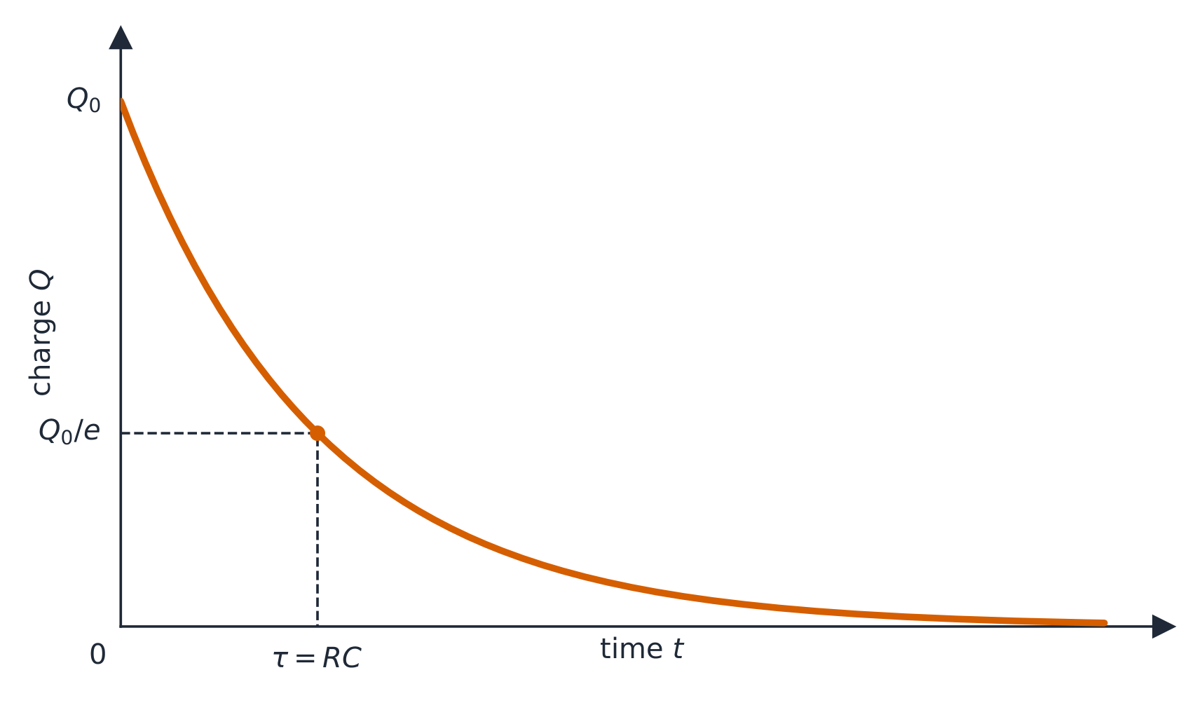
그 해들은 시간 상수(time constant)$\tau=RC$를 포함하는 지수함수입니다:
전류는 첫 순간에 가장 크고 감쇠됩니다 – 콘덴서가 '기다릴' 수 없습니다. 두 한계를 기억하십시오: $t=0$에서 비충전된 콘덴스는 단순한 전선처럼 작동하여 최대 전류를 냅니다. 오랜 시간이 지나면 완전히 충전되어 분기에 전류가 흐르지 않으며, 단선(break)처럼 작동합니다. 어떤 정상 상태(steady state) 에서도 콘덴서 분지를 손가락으로 덮고 저항 회로를 푼 후, 콘덴서가 병렬로 연결된 요소의 전압을 읽으십시오.
정전기 용도에 축적된 전하가 방전될 때 지수함수적으로 감쇠됨
Worked example.$R=5.0\ \text{k}\Omega$, $C=200\ \mu\text{F}$, 그리고 $10\ \text{V}$ 배터리가 있을 때: $\tau=RC=1.0\ \text{s}$; 초기 전류는 $\dfrac{\varepsilon}{R}=2.0\ \text{mA}$; 하나의 시간 상수 후 전하량은 $q=CV(1-e^{-1})\approx1.3\times10^{-3}\ \text{C}$이며, 완전 충전의 약 $63\%$이고, 전류는 초기값의 $37\%$로 떨어졌습니다.
*브레드보드 위 실제 회로: 저항기와 콘덴서가 결합하여 전압 상승 및 하강 속도를 결정합니다
12.1.A
Describe the properties of a magnetic field.
12.1.A.1 A magnetic field is a vector field that can be used to determine the magnetic force exerted on moving electric charges, electric currents, or magnetic materials.
12.1.A.1.i Magnetic fields can be produced by magnetic dipoles or combinations of dipoles, but never by monopoles.
12.1.A.1.ii Magnetic dipoles have north and south polarity.
12.1.A.2 A magnetic field is a vector quantity and can be represented using vector field maps.
12.1.A.3 Magnetic field lines must form closed loops, as described by Gauss's law for magnetism.
12.1.A.3.i Maxwell's equations are the collection of equations that fully describe electromagnetism. Gauss's law for magnetism is Maxwell's second equation.
Equation:$\oint \vec{B} \cdot d\vec{A} = 0$
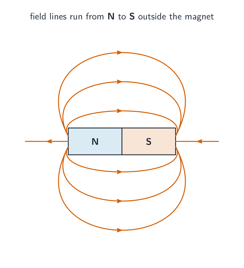
12.1.A.3.ii Magnetic fields in a bar magnet form closed loops, with the external magnetic field pointing away from one end (defined as the north pole) and returning to the other end (defined as the south pole).
12.1.B
Describe the magnetic behavior of a material as a result of the configuration of magnetic dipoles in the material.
12.1.B.1 Magnetic dipoles result from the circular or rotational motion of electric charges. In magnetic materials, this can be the motion of electrons.
12.1.B.1.i Permanent magnetism and induced magnetism are system properties that both result from the alignment of magnetic dipoles within a system.
12.1.B.1.ii No magnetic north pole is ever found in isolation from a south pole. For example, if a bar magnet is broken in half, both halves are magnetic dipoles.
12.1.B.1.iii Magnetic poles of the same polarity will repel; magnetic poles of opposite polarity will attract.
12.1.B.1.iv The magnitude of the magnetic field from a magnetic dipole decreases with increasing distance from the dipole.
12.1.B.2 A magnetic dipole, such as a magnetic compass, placed in a magnetic field will tend to align with the magnetic field.
12.1.B.3 A material's composition influences its magnetic behavior in the presence of an external magnetic field.
12.1.B.3.i Ferromagnetic materials such as iron, nickel, and cobalt can be permanently magnetized by an external field that causes the alignment of magnetic domains or atomic magnetic dipoles.
12.1.B.3.ii Paramagnetic materials such as aluminum, titanium, and magnesium interact weakly with an external magnetic field, in that the magnetic dipoles of the material do not remain aligned after the external field is removed.
12.1.B.3.iii All materials have the property of diamagnetism, in that their electronic structure creates a usually weak alignment of the dipole moments of the material opposite the external magnetic field.
12.1.B.4 Earth's magnetic field may be approximated as a magnetic dipole.
12.1.C
Describe the magnetic permeability of a material.
12.1.C.1 Magnetic permeability is a measurement of the amount of magnetization in a material in response to an external magnetic field.
12.1.C.2 Free space has a constant value of magnetic permeability, known as the vacuum permeability $\mu_0$, that appears in equations representing physical relationships.
12.1.C.3 The permeability of matter has values different from that of free space and arises from the matter's composition and arrangement. It is not a constant for a material and varies based on many factors, including temperature, orientation, and strength of the external field.
출처: College Board AP Course and Exam Description
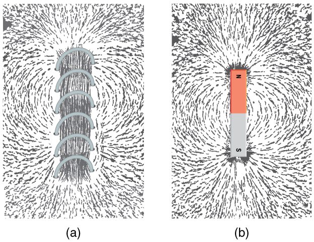
A magnetic field 磁场$\vec{B}$ is a vector field 矢量场 that surrounds magnets, moving charges, and currents; it determines the magnetic force on any moving charge placed in it. Magnetic field lines 磁感线 must form closed loops: they leave the north pole, return to the south pole, and continue through the magnet. Denser lines mean a stronger field.
Field lines run from N to S outside a bar magnet
Closed loops are the content of Gauss's law for magnetism, the second of Maxwell's equations 麦克斯韦方程组:
$$\oint \vec{B}\cdot d\vec{A}=0.$$
The net magnetic flux through any closed surface is zero – as many field lines leave as enter. That is exactly the statement that isolated magnetic monopoles 磁单极子 do not exist. Every source of magnetism is a magnetic dipole 磁偶极子 (a north–south pair), made by circulating charge – in materials, the motion of electrons. Break a bar magnet in half and you get two smaller dipoles, never a lone pole. Like poles repel, opposite poles attract, and a free dipole – a compass 指南针 – rotates to line up with the local field. Earth's own field is approximately a dipole, which is why a compass works. Dipole fields weaken with distance.
How a material responds to an external field depends on how its internal dipoles behave:
Ferromagnetic 铁磁性 (iron, nickel, cobalt): an external field aligns whole magnetic domains 磁畴, and the alignment survives after the field is removed – a permanent magnet.
Paramagnetic 顺磁性 (aluminum, titanium): dipoles align weakly with the field but relax when it is removed.
Diamagnetic 抗磁性 (all materials): the electronic structure produces a usually weak alignment opposite to the field.
The strength of a material's response is its magnetic permeability 磁导率. Free space has the constant value $\mu_0$ (the vacuum permeability); the permeability of matter differs from $\mu_0$ and is not even constant – it varies with temperature, orientation, and field strength.
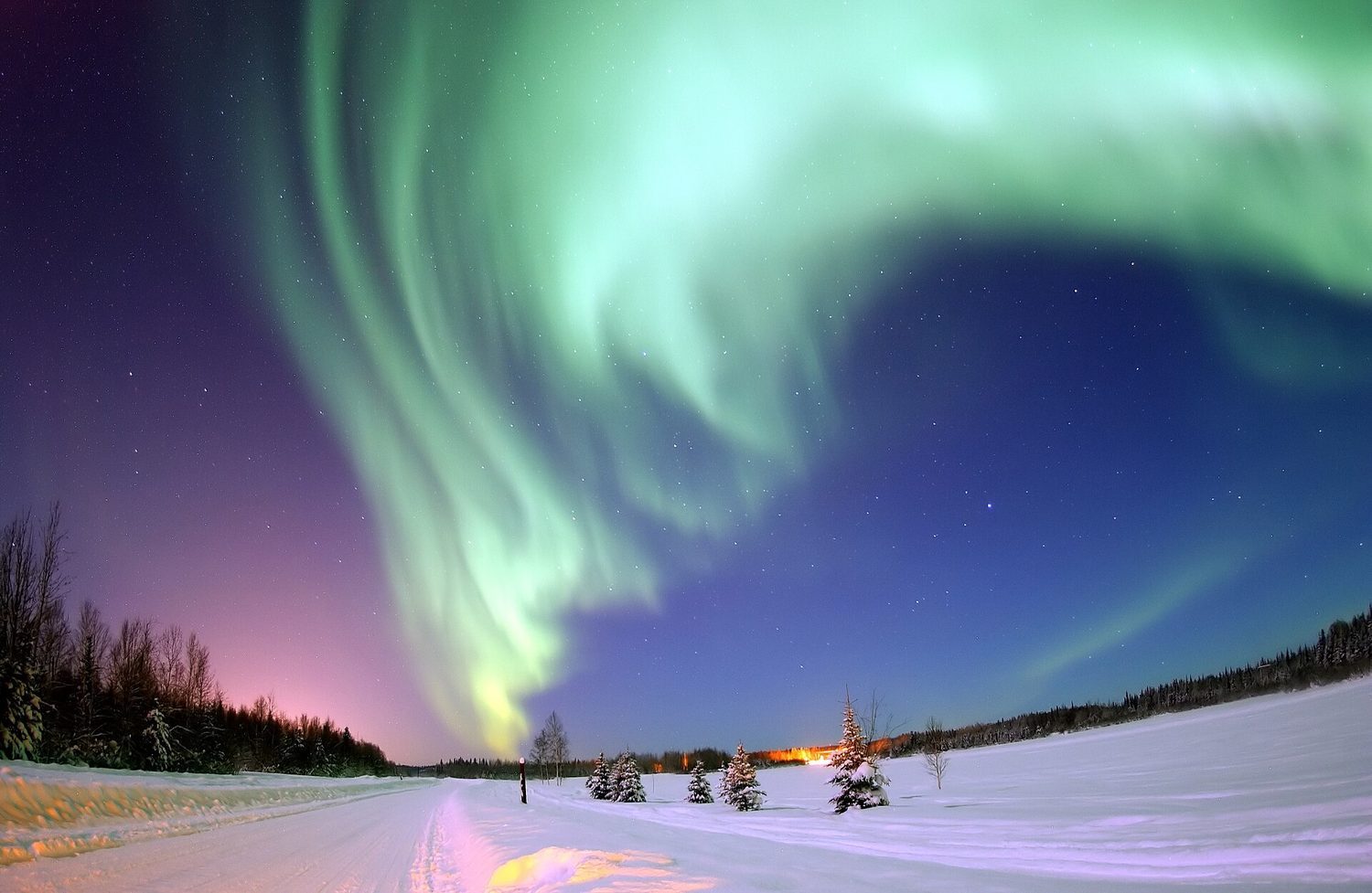
An aurora: charged particles from the Sun are steered by Earth's magnetic field toward the poles
탐색하기
자석의 자기력선 보기
자기장(magnetic field) 선은 자석 외부에서 북극에서 남극으로 향하며, 선들이 빽빽한 곳일수록 자기장이最强합니다.
12.2.B.2 자기장과 전기장이 공존하는 영역에서 이동하는 하전 입자는 각 장으로부터 독립적인 힘을 받는다.
12.2.B.3 홀 효과는 도체 내로 흐르는 하전 입자의 운동 방향과 수직인 성분을 가진 외부 자기장에 의해 도체에 발생되는 전위차에 대한 현상을 설명한다.
출처: College Board AP Course and Exam Description
A moving charge in a magnetic field
A moving charge does two things: it creates a magnetic field, and it feels a force in an external one. The field it creates at a point is perpendicular 垂直 to both its velocity and the position vector from charge to point (right-hand rule again), and is largest where those two are perpendicular – zero directly ahead of or behind the motion.
The force on a charge moving in a field $\vec{B}$ is the cross product
perpendicular to both $\vec{v}$ and $\vec{B}$ – point the fingers of your right hand along $\vec{v}$, curl toward $\vec{B}$, and the thumb gives the force on a positive charge (reverse it for negative). Because $\vec{F}_B\perp\vec{v}$, the magnetic force does no work on the charge: it changes direction, never speed.
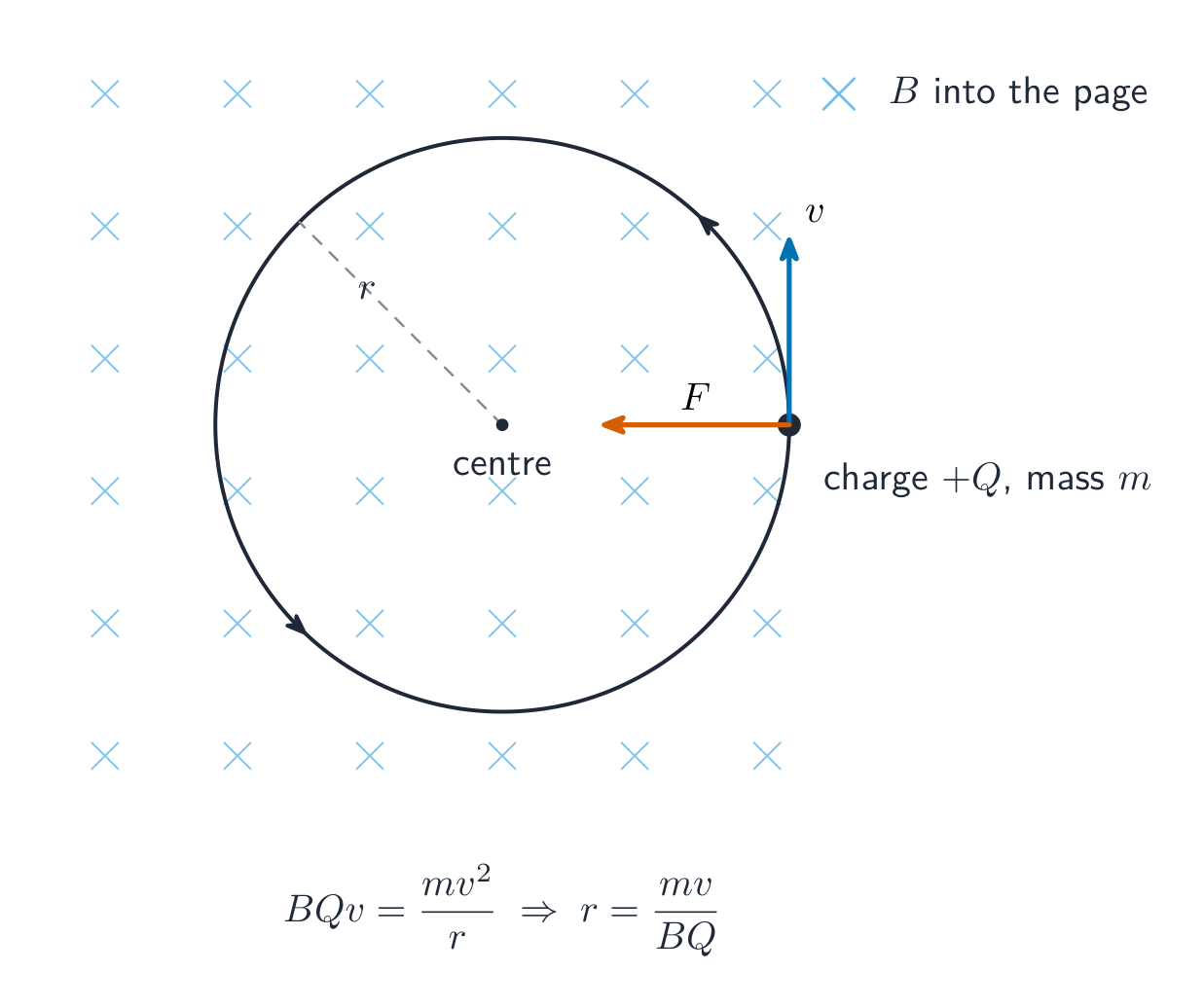
A charge moving perpendicular to a uniform field therefore travels in a circle, the magnetic force supplying the centripetal force 向心力:
Notice the period $T$ does not depend on the speed – faster particles ride larger circles in the same time.
A charged particle moving across a magnetic field follows a circular path
Worked example. A proton ($q=1.6\times10^{-19}\ \text{C}$, $m=1.67\times10^{-27}\ \text{kg}$) enters a $0.50\ \text{T}$ field at $2.0\times10^{5}\ \text{m/s}$, perpendicular to it. The magnetic force $F=qvB=1.6\times10^{-14}\ \text{N}$ bends it into a circle of radius $r=\dfrac{mv}{qB}=\dfrac{1.67\times10^{-27}(2.0\times10^{5})}{1.6\times10^{-19}(0.50)}=4.2\times10^{-3}\ \text{m}$.
In a region with both an electric and a magnetic field, the two forces act independently and add as vectors. Balancing them makes a velocity selector 速度选择器: with $\vec{E}$ and $\vec{B}$ crossed, only charges with $qE=qvB$, i.e. $v=E/B$, pass straight through. The Hall effect 霍尔效应 is the same physics inside a conductor: a field with a component perpendicular to the current pushes the moving carriers sideways, charge builds up on one face, and a measurable potential difference appears across the conductor – its sign reveals whether the carriers are positive or negative.
탐색하기
움직이는 하전하에 작용하는 힘
자기장을 통과하는 하전 입자는 속도 방향과 자기장 방향 모두에 수직인 힘 $F=qvB$를 받습니다. 이것이 모터 효과의 기본 원리입니다. 속도나 자기장 중 하나만 반전시키면 힘의 방향도 반전됩니다.
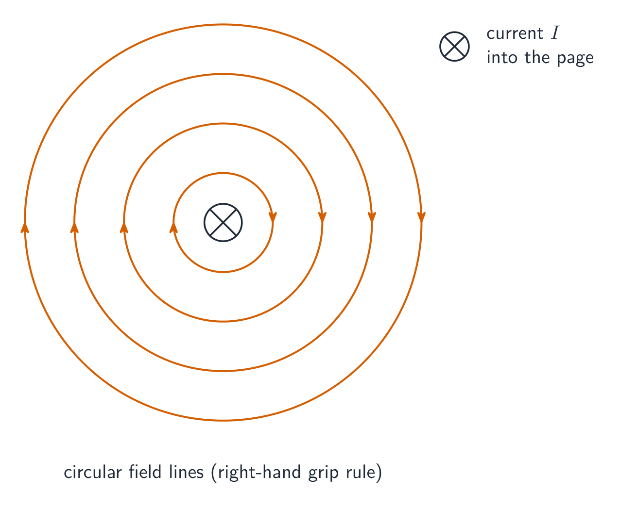
Around any straight segment the field vectors are tangent 相切 to concentric circles 同心圆 centred on the wire – no component toward, away from, or along the wire. Curl your right hand around the wire with the thumb along the current: your fingers give the field direction.
Concentric circular field lines surround a straight current-carrying wire
The Biot–Savart integrals AP expects: a long straight wire ($B=\dfrac{\mu_0 I}{2\pi r}$, or a point on the perpendicular bisector of a finite wire), and the centre of a circular loop,
$$B_{\text{centre of loop}}=\frac{\mu_0 I}{2R},$$
where every element $d\vec{l}$ is perpendicular to $\hat{r}$ and equally distant $R$ – say that in an FRQ derivation. An arc that is a fraction of a full circle contributes that same fraction of $\mu_0 I/2R$ at its centre.
A field also pushes on a current-carrying wire, element by element:
$$\vec{F}_B=\int I\,d\vec{l}\times\vec{B}\qquad(\vec{F}=I\vec{L}\times\vec{B}\ \text{for a straight wire in a uniform field}).$$
Worked example. Two long parallel wires a distance $d=0.10\ \text{m}$ apart each carry $5.0\ \text{A}$ in the same direction. Wire 1's field at wire 2 is $B=\dfrac{\mu_0 I}{2\pi d}=1.0\times10^{-5}\ \text{T}$, so wire 2 feels $\dfrac{F}{L}=I B=5.0\times10^{-5}\ \text{N/m}$, pulled toward wire 1. Same-direction currents attract; opposite currents repel.
A current-carrying coil (solenoid) makes a magnetic field shaped just like a bar magnet's
12.4.A.1.ii 별다른 명시가 없는 한 모든 솔레노이드는 매우 길다고 가정하며, 솔레노이드 내부에는 균일한 자기장이 있고 외부에는 무시할 수 있는 자기장이 있다고 간주한다.
12.4.A.1.iii 암페어 법칙은 긴 솔레노이드 내부의 자기장을 구하는 데 사용할 수 있다.
식:$B_{\text{sol}} = \mu_0 n I$
12.4.A.2 암페어 루프는 전류가 흐르는 도통재周围的 닫힌 경로이다.
12.4.A.3 중첩 원리를 사용하여 공간상 한 점에서의 합성 자기장을 구할 수 있으며, 이는 다양한 조합의 전류 도통재, 도통재 루프, 구간 또는 원통형 도통재에 의해 생성된다.
12.4.A.4 맥스韦尔 방정식은 전자기학을 완전히 기술하는 일련의 방정식이다. 맥스韦尔의 네 번째 방정식은 맥스韦尔 추가항이 포함된 암페어 법칙으로, 자기장은 전기류(암페어 법칙)에 의해 생성될 수 있으며, 변화하는 전기장 역시 움직이는 전하가 자기장을 생성하는 방식과 유사하게 자기장을 생성함(맥스韦尔 추가항)을 나타낸다.
범위 문구: AP 물리학 C: 전기 & 자기에서는 대칭적인 자기장 상황에만 암페어 법칙의 정량적 적용을 요구한다. 긴 직선 도선, 전류를 흐르는 긴 솔레노이드, 그리고 전류 밀도를 갖는 도통재 판 또는 원통형 도통재 등이 AP 물리학 C: 전기 & 자기 시험에서 암페어 법칙이 적용되는 도통재 형태에 해당한다.
범위 문구: AP 물리학 C: 전기 & 자기에서는 변화하는 전기장을 포함하는 맥스韦尔의 네 번째 방정식을 사용하는 것은 요구하지 않는다. 다만, 학생들은 변화하는 전기장이 자기장을 생성함을 이해해야 한다.
출처: College Board AP Course and Exam Description
For symmetric current distributions, Ampère's law 安培定律 finds the field far faster than Biot–Savart:
Choose an Amperian loop 安培环路 that matches the symmetry, so that $B$ is constant along the loop (and parallel to it) and comes out of the integral. AP applies it to long straight wires, long solenoids, and conductors carrying a current density 电流密度 (slabs and cylinders); combinations are handled by superposition 叠加.
Worked example. Find the field $0.10\ \text{m}$ from a long wire carrying $5.0\ \text{A}$. A circular loop of radius $r$ shares the field's symmetry, so $B(2\pi r)=\mu_0 I$ and
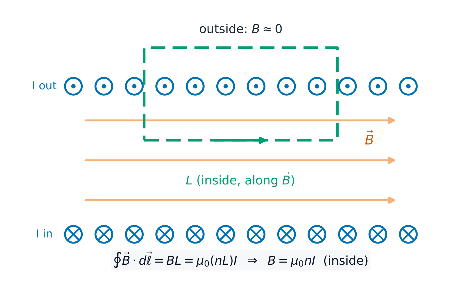
A long solenoid 螺线管 (assumed: uniform field inside, negligible field outside) is the other classic. Take a rectangular loop with one side of length $L$ inside, parallel to the axis: only that side contributes to the integral, so $BL=\mu_0 (nL) I$ and
$$B_{\text{sol}}=\mu_0 n I,$$
with $n$ the turns per metre.
A rectangular Amperian loop derives the uniform field inside a solenoid
Worked example (cylinder). A solid cylindrical conductor of radius $R$ carries current $I$ spread uniformly over its cross-section. Inside ($r), a circular loop encloses $I_{\text{enc}}=I\dfrac{r^2}{R^2}$, so $B=\dfrac{\mu_0 I r}{2\pi R^2}$ – the field grows linearly to the surface, then falls off as $1/r$ outside.
Exam skill. Every Ampère's-law answer earns its marks in the setup: name the loop, state why$B$ is constant and parallel to it (symmetry), and count $I_{\text{enc}}$ carefully before you solve. Maxwell's fourth equation adds one more idea you should know qualitatively: a changing electric field also creates a magnetic field – but AP will not ask you to compute with that term.
The magnetic force $\vec F=q\vec v\times\vec B$ is perpendicular to velocity — use the right-hand rule and note it does no work.
A charge in a uniform field moves in a circle with $r=\tfrac{mv}{qB}$.
Find the field of currents with Biot–Savart$d\vec B=\tfrac{\mu_0}{4\pi}\tfrac{I\,d\vec l\times\hat r}{r^2}$ or Ampère's law$\oint \vec B\cdot d\vec l=\mu_0 I_{enc}$ when there is symmetry.
Force on a wire is $\vec F=I\vec L\times\vec B$; keep the cross-product direction straight.
Distinguish the force on a charge from the field the current creates.
13.1.A
Describe the magnetic flux through an arbitrary area or geometric shape.
13.1.A.1 For a magnetic field $\vec{B}$ that is constant across an area $\vec{A}$, the magnetic flux through the area is defined as $\Phi_B = \vec{B} \cdot \vec{A}$ .
13.1.A.1.i The area vector is defined as perpendicular to the plane of the surface and outward from a closed surface.
13.1.A.1.ii The sign of flux is given by the dot product of the magnetic field vector and the area vector.
13.1.A.2 The total magnetic flux passing through a surface is defined by the surface integral of the magnetic field over the surface area.
Magnetic flux 磁通量 measures how much magnetic field passes through a surface. For a uniform field through a flat loop it is the dot product $\Phi_B=\vec{B}\cdot\vec{A}=BA\cos\theta$; in general it is the surface integral 面积分
$$\Phi_B=\int \vec{B}\cdot d\vec{A}.$$
The area vector 面积矢量 is perpendicular to the surface (outward from a closed one), and the sign of the flux comes from the dot product. Flux changes if $B$ changes, the area changes, or the loop turns – keep all three routes in mind, because each one is an exam question.
13.2.A.1.i When the area of the surface being considered is constant, the induced emf is equal to the area multiplied by the rate of change in the component of the magnetic field perpendicular to the surface.
13.2.A.1.ii When the magnetic field is constant, the induced emf is equal to the magnetic field multiplied by the rate of change in area perpendicular to the magnetic field.
13.2.A.1.iii When an emf is induced in a long solenoid, the total induced emf is equal to the induced emf in a single loop multiplied by the number of loops in the solenoid.
13.2.A.2 Lenz's law is used to determine the direction of an induced emf resulting from a changing magnetic flux.
13.2.A.2.i An induced emf generates a current that creates a magnetic field that opposes the change in magnetic flux.
13.2.A.2.ii The right-hand rule is used to determine the relationships between current, emf, and magnetic flux.
13.2.A.3 Maxwell's equations are the collection of equations that fully describe electromagnetism. Maxwell's third equation is Faraday's law of induction, which describes the relationship between a changing magnetic flux and an induced electric field.
13.2.A.4 Maxwell's equations can be used to show that electric and magnetic fields obey wave equations and that electromagnetic waves travel at a constant speed in free space.
Boundary statement: AP Physics C: Electricity & Magnetism does not expect students to mathematically derive the speed of light in free space from Maxwell's equations. This relationship is included above solely as an indication of the further applications, implications, and connections to physical phenomena that students may study in more advanced physics courses.
출처: College Board AP Course and Exam Description
Electromagnetic induction
A changing flux induces an emf 电动势 – Faraday's law 法拉第定律:
$$\varepsilon=-\frac{d\Phi_B}{dt}.$$
With constant area, $\varepsilon=-A\,\dfrac{dB_\perp}{dt}$; with constant field, $\varepsilon=-B\,\dfrac{dA_\perp}{dt}$. A coil of $N$ turns multiplies the single-loop emf: $|\varepsilon_{\text{sol}}|=N\left|\dfrac{d\Phi_B}{dt}\right|$.
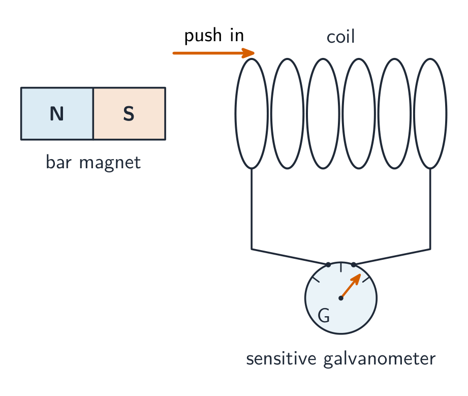
Lenz's law 楞次定律 is the minus sign: the induced current 感应电流 flows so that its own magnetic field opposes the change in flux that created it. Push a magnet toward a loop and the loop pushes back; pull it away and the loop pulls it in. Use the right-hand rule 右手定则 to turn "oppose the change" into a current direction.
Moving a magnet into a coil induces an e.m.f. that drives a current
A rod of length $L$ sliding at speed $v$ across a field is the special case worth memorising – the motional emf 动生电动势$\varepsilon=BLv$.
Worked example. A $0.20\ \text{m}$ rod slides at $3.0\ \text{m/s}$ across a $0.50\ \text{T}$ field: $\varepsilon=BLv=0.50(0.20)(3.0)=0.30\ \text{V}$. Equivalently, if a single loop's flux drops from $0.020\ \text{Wb}$ to $0.008\ \text{Wb}$ in $0.030\ \text{s}$, the average emf is $\varepsilon=\dfrac{0.012}{0.030}=0.40\ \text{V}$.
Faraday's law is also the third of Maxwell's equations 麦克斯韦方程组, in a deeper form: a changing magnetic flux creates a circulating electric field, $\oint\vec{E}\cdot d\vec{l}=-\dfrac{d\Phi_B}{dt}$ – that field is what pushes the charges around the loop. Together, Maxwell's equations predict electromagnetic waves 电磁波 travelling at $c=1/\sqrt{\varepsilon_0\mu_0}$ (you should know this connection, but AP will not ask you to derive it).
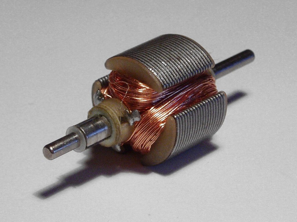
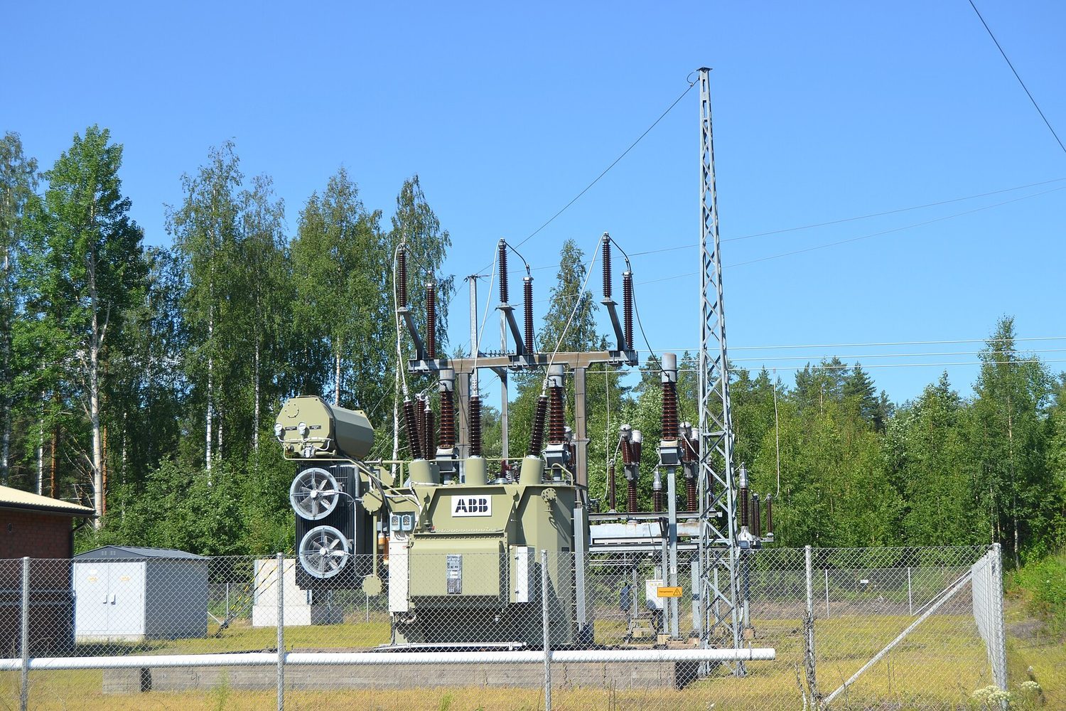
Coils of wire spinning in a magnetic field: moving them past the field induces a current, the basis of a generatorA substation transformer: changing magnetic flux in coils induces the voltages that power the grid
탐색하기
자석을 움직여 전류 유도하기
코일을 지나가는 **자기 플럭스(magnetic flux)**가 변화하면 기전력(EMF)이 유도됩니다(패러데이의 법칙). 그 방향은 변화에 반대됩니다(렌츠의 법칙). 자석을 더 빠르게 움직이면 더 큰 EMF가 발생합니다.
13.3.A
Describe the force exerted on a conductor due to the interaction between an external magnetic field and an induced current within that conductor.
13.3.A.1 When an induced current is created in a conductive loop, the already-present magnetic field will exert a magnetic force on the moving charge carriers within the loop.
13.3.A.2 When current is induced in a conducting loop, magnetic forces are only exerted on the segments of the loop that are within the external magnetic field. These magnetic forces may cause translational or rotational acceleration.
13.3.A.3 The force on a conducting loop is proportional to the induced current in the loop, which depends on the rate of change of magnetic flux, the resistance of the loop, and the velocity of the loop.
13.3.A.4 Newton's second law can be applied to a conducting loop moving in a magnetic field as it experiences an induced emf.
출처: College Board AP Course and Exam Description
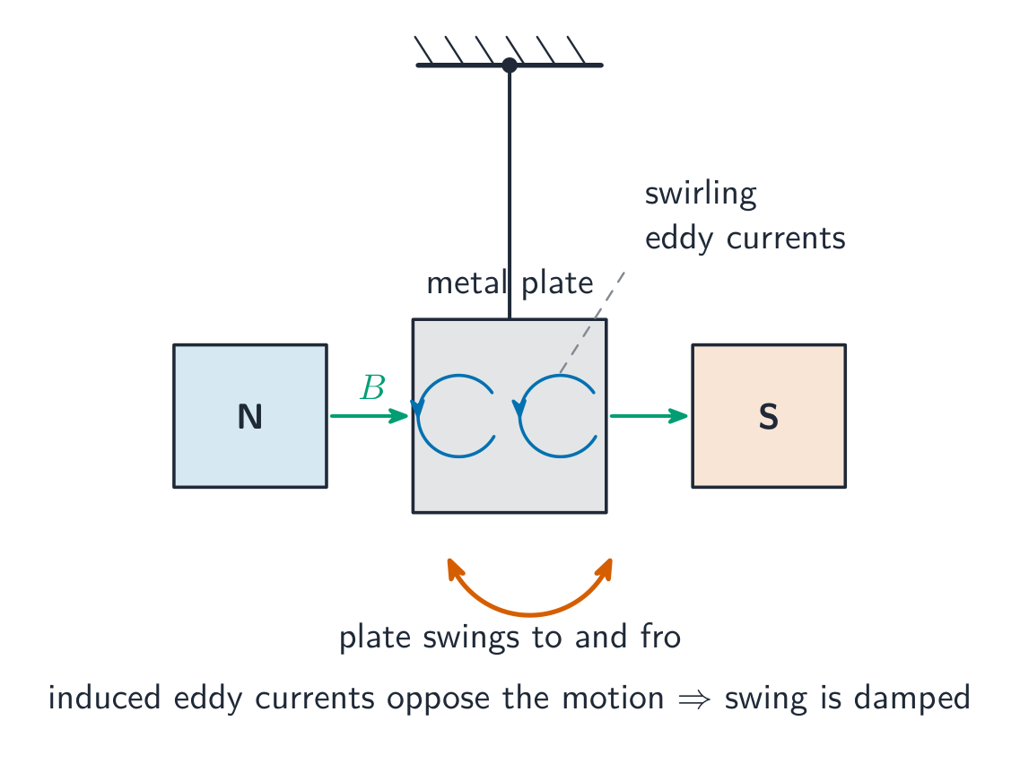
Once an induced current flows, the external field exerts forces on it ($\vec{F}=\int I\,d\vec{l}\times\vec{B}$) – and by Lenz's law those forces always resist the motion that causes the induction. Only the segments of the loop actually inside the field feel a force, which can make a loop accelerate, rotate, or brake. This is the origin of eddy currents 涡电流 braking, and you can apply Newton's second law to a moving loop or rod like any other mechanics problem.
Induced eddy currents oppose motion, quickly damping a metal plate swinging in a field
The classic setup is a rod sliding on conducting rails connected by a resistor:
A rod sliding on rails: the induced current feels a force opposing the motion
Worked example (the full chain). Rails $L=0.20\ \text{m}$ apart with resistance $R=0.60\ \Omega$ sit in a $0.50\ \text{T}$ field into the page. The rod is pushed at a constant $3.0\ \text{m/s}$. Then: $\varepsilon=BLv=0.30\ \text{V}$; $I=\varepsilon/R=0.50\ \text{A}$; the field pushes back on the rod with $F=BIL=0.50(0.50)(0.20)=0.050\ \text{N}$. The pushing force does work at $P=Fv=0.15\ \text{W}$ – exactly the $P=I^2R=0.15\ \text{W}$ dissipated in the resistor. Mechanical work becomes electrical energy: that is a generator 发电机, and energy is conserved. Released with no push, the rod slows exponentially: $ma=-\dfrac{B^2L^2}{R}v$.
Exam skill. FRQs walk this exact chain: flux $\to$ emf $\to$ current $\to$ force $\to$ Newton's second law. Write each link separately and check the direction with Lenz's law at the end.
13.4.A.2.i 인덕터에 전류가 흐를 때 생성된 자기장에 저장된 에너지는 저항기를 통해 소모되거나 콘덴서를 충전하는 데 사용될 수 있다.
13.4.A.2.ii 인덕터에서 생성된 에너지를 다른 형태의 에너지로 전달하는 과정은 보존 법칙을 따른다.
13.4.A.3 인덕터에 패러데이의 법칙을 적용하고 인덕턴스의 정의를 사용하여 유도 기전력을 인덕턴스와 전류의 변화율과 연관시킬 수 있다.
식:$\mathcal{E}_i = -L\dfrac{dI}{dt}$
출처: College Board AP Course and Exam Description
Inductance 电感 is a conductor's tendency to oppose a change in its own current: changing current changes its own flux, which self-induces an emf. From Faraday's law,
$$\varepsilon=-L\frac{dI}{dt}.$$
An inductor 电感器 is a circuit element built to have large inductance – usually a solenoid 螺线管, where geometry gives
with $N$ total turns, area $A$, length $\ell$, and the magnetic permeability 磁导率 of the core. (Straight wires are modelled as having zero inductance.) An inductor carrying current $I$ stores energy in its magnetic field:
$$U_L=\tfrac{1}{2}LI^2,$$
which can later be dissipated in a resistor or moved into a capacitor – conservation of energy applies as usual.
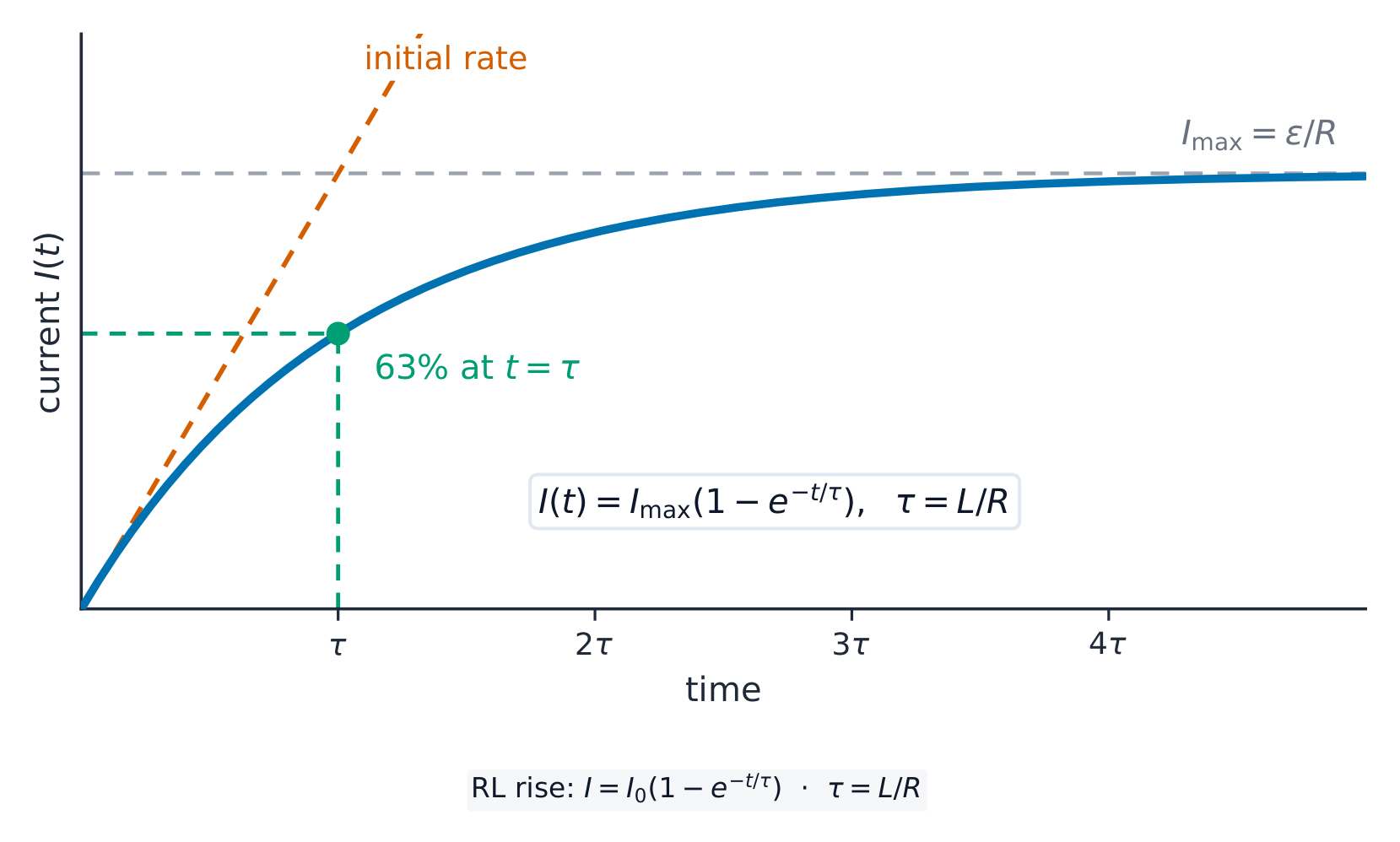
The time constant 时间常数$\tau$ sets the pace: after one $\tau$ a rising current reaches about $63\%$ of its final value (a decaying one falls to $37\%$); it is also how long the change would take at the initial rate. Learn the two limits – they answer most conceptual questions:
Just after the switch closes ($t=0$): current cannot jump, so the inductor momentarily blocks it, self-inducing an emf equal and opposite to the applied potential difference.
Long after ($t\gg\tau$): the current is steady, $dI/dt=0$, and the inductor behaves as a plain wire – the exact opposite of a capacitor.
The current in an RL circuit rises exponentially, reaching 63% at one time constant
Worked example.$\varepsilon=12\ \text{V}$, $R=6.0\ \Omega$, $L=3.0\ \text{H}$: final current $\varepsilon/R=2.0\ \text{A}$, $\tau=L/R=0.50\ \text{s}$. At $t=0.50\ \text{s}$ the current is $2.0(1-e^{-1})\approx1.3\ \text{A}$. At $t=0$ the inductor's potential difference is the full $12\ \text{V}$; as $t\to\infty$ it falls to zero. Current, inductor voltage, and stored energy are all exponential in time.
학습 목표 13.6.A: 정전용기와 단일 인덕터가 조합된 회로의 물리적 및 전기적 특성을 설명한다.
13.6.A.1 충전된 정전용기와 인덕터만 포함된 회로(LC 회로)에서 인덕터의 최대 전류는 회로 내 에너지 보존 법칙을 사용하여 구할 수 있다.
13.6.A.2 LC 회로에서 정전용기에 저장된 전하의 시간 의존성은 단순 조화 운동으로 모델링할 수 있다.
식(유도):$\dfrac{d^2 q}{dt^2} = -\dfrac{1}{LC} q$
13.6.A.3 진동하는 LC 회로의 각주파수는 LC 회로를 기술하는 미분방정식으로부터 유도될 수 있다.
식(유도):$\omega = \dfrac{1}{\sqrt{LC}}$
출처: College Board AP Course and Exam Description
LC circuit: energy sloshes like a spring
An LC circuit LC电路 has no resistance, so nothing dissipates energy: it oscillates 振荡, sloshing energy between the capacitor's electric field and the inductor's magnetic field. The loop rule gives
$$\frac{d^2q}{dt^2}=-\frac{1}{LC}\,q,$$
the same equation as a mass on a spring – simple harmonic motion 简谐运动 with charge playing the role of displacement and
$$\omega=\frac{1}{\sqrt{LC}}.$$
The total energy $\dfrac{q^2}{2C}+\tfrac12LI^2$ stays constant: all in the capacitor at maximum charge, all in the inductor at maximum current.
Worked example.$L=2.0\ \text{H}$, $C=8.0\ \mu\text{F}$: $\omega=\dfrac{1}{\sqrt{2.0(8.0\times10^{-6})}}=250\ \text{rad/s}$, period $T=2\pi/\omega\approx0.025\ \text{s}$. If the capacitor starts charged to $12\ \text{V}$, then $U=\tfrac12CV^2=5.8\times10^{-4}\ \text{J}$, and the maximum current follows from $\tfrac12LI_{\max}^2=U$: $I_{\max}=\sqrt{2U/L}=0.024\ \text{A}$ – conservation of energy 能量守恒, no calculus needed.

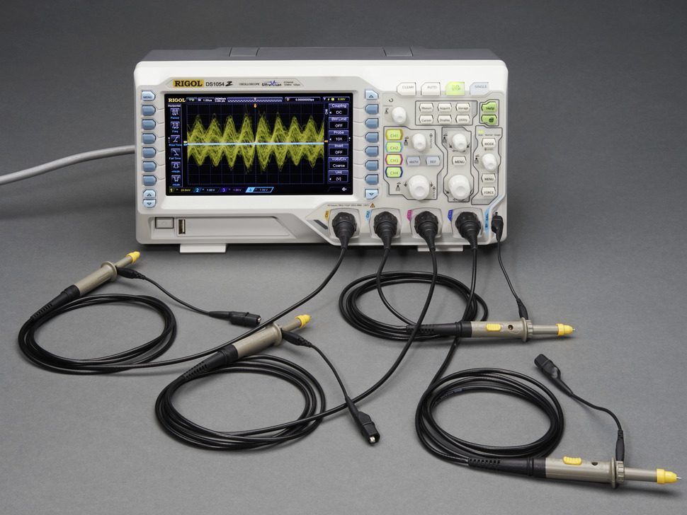
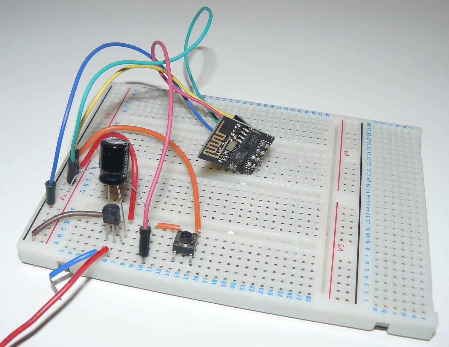 *브레드보드 위 실제 회로: 저항기와 콘덴서가 결합하여 전압 상승 및 하강 속도를 결정합니다