| Learning Objective | Essential Knowledge |
|---|---|
9.1.A |
|
Electric Potential
AP Physics C: Electricity and Magnetism · Topic 9
 8:02
8:02
Electric Potential
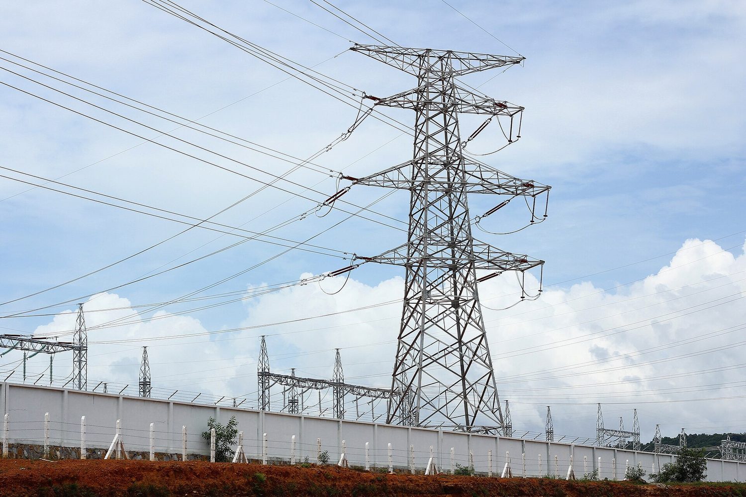
Look at these numbers. A small battery says one point five volts. A car battery says twelve. A high-voltage transmission line carries four hundred thousand. A…
English narration · English + 中文 subtitles burned in
9.1
Electric Potential Energy
Syllabus
Source: College Board AP Course and Exam Description
When you push two like charges together, you do work 功 against the electric force. That work is stored by the pair as electric potential energy 电势能:
$$U_E=\frac{1}{4\pi\varepsilon_0}\frac{q_1 q_2}{r}=k\frac{q_1 q_2}{r}.$$
$U_E$ is defined as the work an external force must do to bring the charges from infinitely far away to a distance $r$ apart. The signs carry the physics:
- Like charges: $U_E>0$. An outside push was needed to bring them together. If released, they fly apart, and the stored energy becomes kinetic energy 动能.
- Opposite charges: $U_E<0$. The pair is bound. You must supply $|U_E|$ of work to pull them apart to infinity.
The electric force is a conservative force 保守力: the work it does depends only on the start and end points, not the path, and equals $-\Delta U_E$.
For a system 系统 of several charges, add the potential energy of every distinct pair:
$$U_{\text{total}}=k\!\left(\frac{q_1q_2}{r_{12}}+\frac{q_1q_3}{r_{13}}+\frac{q_2q_3}{r_{23}}\right).$$
Worked example. Three $+2.0\ \mu\text{C}$ charges sit at the corners of an equilateral triangle with sides $0.30\ \text{m}$. Each pair stores $U=\dfrac{kq^2}{r}=\dfrac{(9.0\times10^{9})(2.0\times10^{-6})^2}{0.30}=0.12\ \text{J}$. There are three pairs, so $U_{\text{total}}=3\times0.12\ \text{J}=0.36\ \text{J}$. This is the work needed to assemble the triangle from infinity – and the kinetic energy the charges would share if all three were released.
Vocabulary
Train
| English |
|---|
| work/wɜːk/ |
| electric potential energy/ɪˈlektrɪk pəˈtenʃl ˈenədʒi/ |
| kinetic energy/kɪˈnetɪk ˈenədʒi/ |
| conservative force/kənˈsɜːvətɪv fɔːs/ |
| system/ˈsɪstəm/ |
9.2
Electric Potential
Syllabus
| Learning Objective | Essential Knowledge |
|---|---|
9.2.A |
Boundary statement: AP Physics C: Electricity & Magnetism only expects students to use calculus to find the electric potential resulting from the following charge distributions and locations: an infinitely long, uniformly charged wire or cylinder at a distance from its central axis, a thin ring of charge at a location along the axis of the ring, a semicircular arc or part of a semicircular arc at its center, and a finite wire or line charge at a point collinear with the line charge or at a location along its perpendicular bisector. |
9.2.B |
|
Source: College Board AP Course and Exam Description
Electric potential 电势 is electric potential energy per unit charge at a point in space. It is measured in volts ($1\ \text{V}=1\ \text{J/C}$):
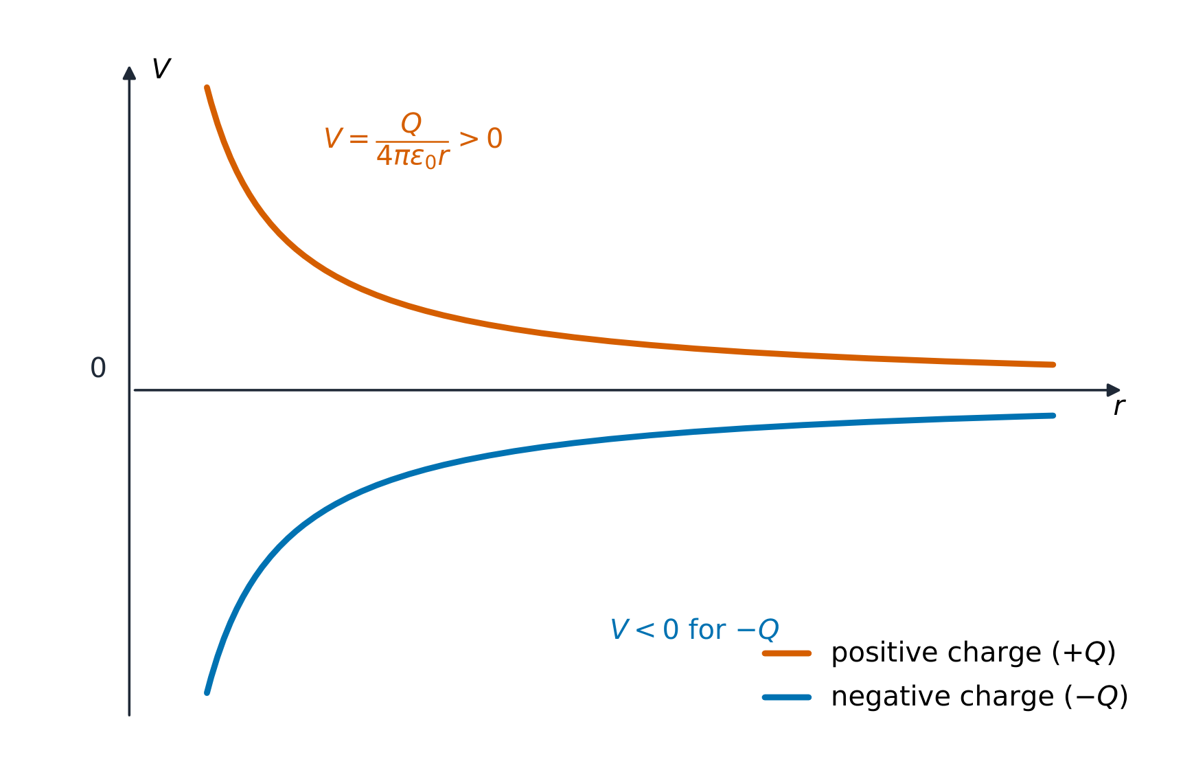
$$V=\frac{U_E}{q},\qquad V=\frac{1}{4\pi\varepsilon_0}\frac{q}{r}\ \text{(point charge)}.$$
Potential is a scalar 标量: it has a sign but no direction. This makes $V$ far easier to work with than the field $\vec{E}$. For several point charges 点电荷, use scalar superposition 叠加 – add the potentials with their signs:
$$V=\frac{1}{4\pi\varepsilon_0}\sum_i \frac{q_i}{r_i}.$$
Worked example. The potential $0.10\ \text{m}$ from a $+3.0\ \text{nC}$ point charge is $V=\dfrac{kq}{r}=\dfrac{9.0\times10^{9}(3.0\times10^{-9})}{0.10}=270\ \text{V}$. Now add a $-3.0\ \text{nC}$ charge $0.30\ \text{m}$ from the same point: it contributes $\dfrac{9.0\times10^{9}(-3.0\times10^{-9})}{0.30}=-90\ \text{V}$, so the total is $270-90=180\ \text{V}$. Just a signed sum – no vector components to resolve.
Continuous charge distributions
For a continuous charge distribution 连续电荷分布, cut it into small pieces $dq$, treat each piece as a point charge, and integrate 积分:
$$V=\frac{1}{4\pi\varepsilon_0}\int\frac{dq}{r}.$$
This is a scalar integral, so it is usually much easier than the field integral. AP expects you to handle four shapes with calculus: a thin ring (at a point on its axis), an arc (at its centre), a finite line or wire (collinear, or on its perpendicular bisector), and an infinitely long wire or cylinder (at a distance from its axis).
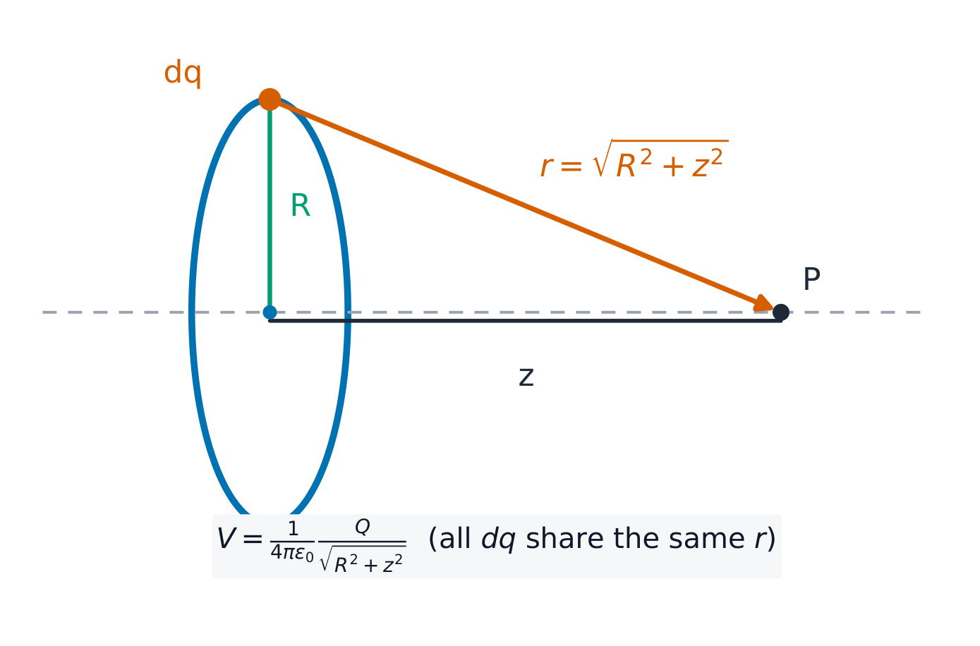
Worked example (ring of charge). A thin ring of radius $R$ carries total charge $Q$. For a point $P$ on the axis a distance $z$ from the centre, every element $dq$ sits at the same distance $r=\sqrt{R^2+z^2}$ from $P$. The distance is constant, so it comes out of the integral:
$$V=\frac{1}{4\pi\varepsilon_0}\int\frac{dq}{\sqrt{R^2+z^2}}=\frac{1}{4\pi\varepsilon_0}\frac{Q}{\sqrt{R^2+z^2}}.$$
On an FRQ, say that $r$ is the same for every element – that statement is the marked step. The same idea gives $V=kQ/R$ at the centre of any arc, whatever its angle.
From potential to field
Potential and field contain the same information, linked by a derivative in each direction and by a path integral:
$$E_x=-\frac{dV}{dx},\qquad \Delta V=V_b-V_a=-\int_a^b \vec{E}\cdot d\vec{r}.$$
The field is the negative gradient 梯度 of the potential: $\vec{E}$ points from high potential to low potential, "downhill". Where $V$ changes quickly, the field is strong.
Worked example. Along the $x$-axis, $V(x)=3x^{2}-2x$ (volts, with $x$ in metres). Then $E_x=-\dfrac{dV}{dx}=2-6x\ \text{V/m}$. At $x=0.50\ \text{m}$, $E_x=-1.0\ \text{V/m}$: the field there points in the $-x$ direction.
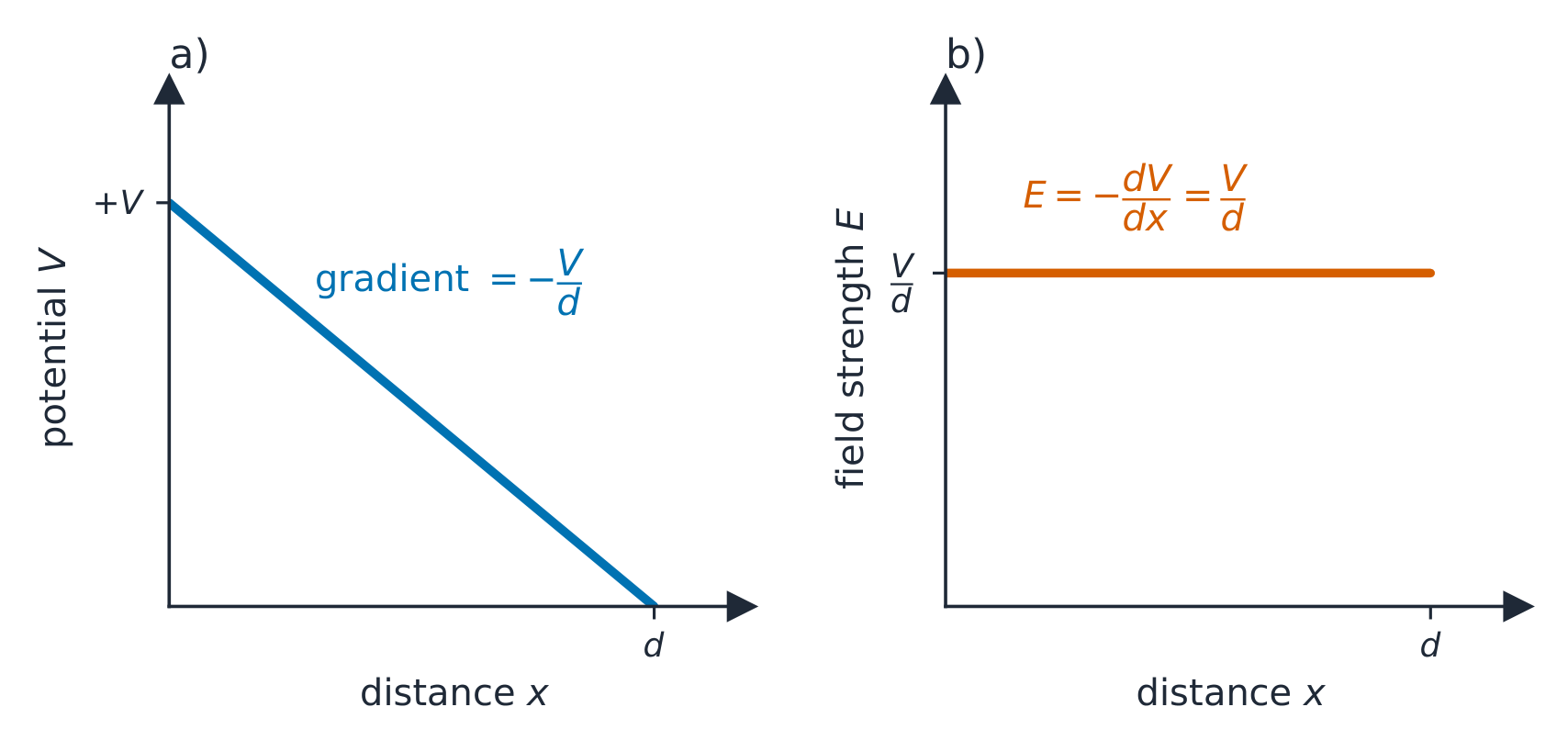
The potential difference 电势差 between two points is the change in potential energy per unit charge moved between them: $\Delta V=\Delta U_E/q$. A battery makes a potential difference chemically: reactions inside separate positive from negative charge and hold the terminals a fixed $\Delta V$ apart.
Equipotential maps
An equipotential 等势面 line (also called an isoline 等值线) joins points that share the same potential. Four rules let you read any map:
- Isolines are perpendicular 垂直 to field lines 电场线 everywhere they cross.
- $\vec{E}$ points from high $V$ to low $V$ – never along an isoline. Moving a charge along an isoline takes no work.
- Closely spaced isolines mean a strong field: $E\approx-\Delta V/\Delta x$.
- You can sketch the field map from an isoline map, and the isoline map from a field map.

Exam skill. Given a map with isolines every $10\ \text{V}$ spaced about $2\ \text{cm}$ apart, estimate $E\approx\dfrac{10}{0.02}=500\ \text{V/m}$, pointing from the higher-value line to the lower one. The work an external agent does moving a charge $q$ slowly from $A$ to $B$ is $W=q(V_B-V_A)$ – the path taken does not matter.
Explore
Field lines and the potential around a charge
Electric potential is the energy per unit charge. It falls off with distance from a positive charge; the field lines point from high potential to low.
Vocabulary
Train
| English |
|---|
| Electric potential/ɪˈlektrɪk pəˈtenʃl/ |
| scalar/ˈskeɪlə/ |
| point charges/pɔɪnt ˈtʃɑːdʒɪz/ |
| superposition/ˌsuːpəpəˈzɪʃn/ |
| continuous charge distribution/kənˈtɪnjuːəs tʃɑːdʒ ˌdɪstrɪˈbjuːʃn/ |
| integrate/ˈɪntɪɡreɪt/ |
| gradient/ˈɡreɪdɪənt/ |
| potential difference/pəˈtenʃl ˈdɪfrəns/ |
| equipotential/ˌiːkwɪpəˈtenʃl/ |
| isoline/ˈaɪsəliːn/ |
| perpendicular/ˌpɜːpənˈdɪkjʊlə/ |
| field lines/fiːld laɪnz/ |
9.3
Conservation of Electric Energy
Syllabus
| Learning Objective | Essential Knowledge |
|---|---|
9.3.A |
|
Source: College Board AP Course and Exam Description
When a charge $q$ moves between two points that differ in potential by $\Delta V$, the potential energy of the charge–field system changes by
$$\Delta U_E=q\,\Delta V.$$
If only the electric force acts, total energy is conserved, so the kinetic energy changes by the opposite amount:
$$\Delta K=-\Delta U_E=-q\,\Delta V.$$
Watch the two signs together: a positive charge speeds up when it moves to lower potential, while a negative charge speeds up when it moves to higher potential. Both are just the system trading potential energy for kinetic energy. This is how particle accelerators give charged particles their energy, and it underlies energy analysis in circuits.
Worked example. A proton ($q=1.6\times10^{-19}\ \text{C}$, $m=1.67\times10^{-27}\ \text{kg}$) starts at rest and is accelerated through a potential drop of $500\ \text{V}$ (it moves to lower potential, so $\Delta V=-500\ \text{V}$ and $\Delta K=-q\,\Delta V=+8.0\times10^{-17}\ \text{J}$). Setting $\Delta K=\tfrac12 mv^2$:
$$v=\sqrt{\frac{2(8.0\times10^{-17})}{1.67\times10^{-27}}}=3.1\times10^{5}\ \text{m/s}.$$
Exam skill. Choose energy methods, not kinematics, whenever the field is non-uniform or the path curves: only the end-point potentials matter. A typical FRQ chain is $q\,\Delta V \to \Delta K \to v$, with one line of justification: "the electric force is conservative, so energy is conserved."
9.3
Exam tips
- Relate field and potential by $V=-\int \vec E\cdot d\vec l$ and $\vec E=-\nabla V$ (in 1-D, $E_x=-\tfrac{dV}{dx}$).
- Potential is a scalar — add contributions with signs, no vector components needed.
- Potential energy of a pair is $U=\tfrac{1}{4\pi\varepsilon_0}\tfrac{q_1 q_2}{r}$; use energy conservation for a charge's speed.
- Know that no work is done moving along an equipotential, which is perpendicular to $\vec E$.
- Choose the zero of potential (usually infinity) and state it.
Interactive lessons on this topic
Work through it step by step, with instant-check exercises.