National Income and Price Determination · ⁨国民所得および価格決定⁩

AP Macroeconomics · ⁨AP マクロ経済学⁩ · Topic 3 · ⁨トピック 3⁩

View Slides · ⁨查看幻灯片⁩ Train · ⁨練習する⁩

Video lesson for this topic · ⁨このトピックのビデオレッスン⁩ Open the video page · ⁨動画ページを開く⁩

3.1

Aggregate Demand · ⁨総需要⁩

Syllabus · ⁨シラバス⁩

English

Enduring Understanding (MOD-2): Economists use the aggregate demand–aggregate supply model to represent the relationship between the price level and aggregate output in an economy and to illustrate how output, employment, and the price level respond to macroeconomic shocks.

Learning Objective MOD-2.A: a. Define (using graphs as appropriate) the aggregate demand (AD) curve. b. Explain (using graphs as appropriate) the slope of the AD curve and its determinants.

MOD-2.A.1 The aggregate demand (AD) curve describes the relationship between the price level and the quantity of goods and services demanded by households (consumption), firms (investment), government (government spending), and the rest of the world (net exports).
MOD-2.A.2 The negative slope of the AD curve is explained by the real wealth effect, the interest rate effect, and the exchange rate effect. [See EK MKT-3.A.1]
MOD-2.A.3 Any change in the components of aggregate demand (consumption, investment, government spending, or net exports) that is not due to changes in the price level leads to a shift of the AD curve.

日本語

持続的認識（MOD-2）： 経済学者は、価格水準と経済内の総生産量の関係を表現し、マクロ経済ショックに対する生産量、雇用、および価格水準の反応を示すために、総需要・総供給モデルを使用する。

学習目標 MOD-2.A: a. 総需要（AD）曲線を定義せよ（必要な場合は図を用いる）。 b. AD曲線の傾きとその決定要因を説明せよ（必要な場合は図を用いる）。

MOD-2.A.1 総需要（AD）曲線は、価格水準と、家計（消費）、企業（投資）、政府（政府支出）、および国外（純輸出）が要求する財・サービスの数量との関係を表す。
MOD-2.A.2 AD曲線の負の傾きは、実質富効果、利子率効果、為替レート効果によって説明される。[EK MKT-3.A.1参照]
MOD-2.A.3 価格水準の変化に起因しない総需要の構成要素（消費、投資、政府支出、または純輸出）の変化は、AD曲線のシフトをもたらす。

Source: College Board AP Course and Exam Description · ⁨出典: College Board AP コースおよび試験説明書⁩

English

The AD–AS model: a demand shock

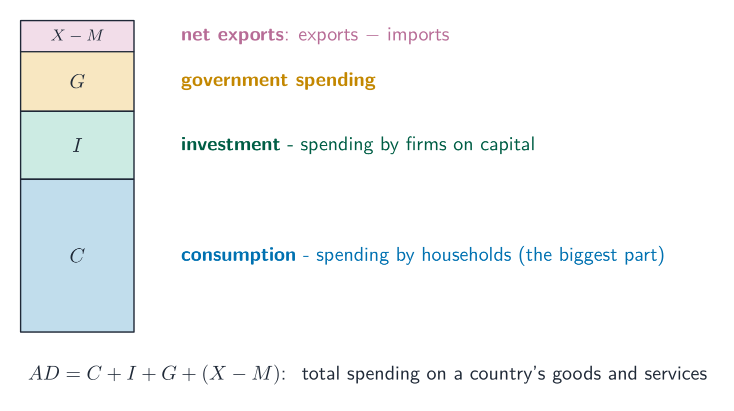
Aggregate demand (AD) 总需求 shows the total quantity of real output ($C+I+G+X_n$) buyers want at each price level 价格水平. It slopes downward for three reasons special to the whole economy:

the wealth effect 财富效应 (a higher price level shrinks the real value of money, so people buy less),
the interest-rate effect 利率效应 (a higher price level raises money demand and interest rates, cutting investment),
the net-export effect (a higher domestic price level makes exports dearer and imports cheaper).

A change in the price level is a movement along AD. AD shifts when any component of $C+I+G+X_n$ changes for another reason – consumer confidence, business expectations, government spending, taxes, or foreign incomes.

日本語

都市のスカイライン: 国民総生産と総需要は経済全体での支出を反映する

AD-ASモデル：需要ショック

総需要 (AD) は、各物価水準において買い手が求める実質生産量（$C+I+G+X_n$）の総量を示します。経済全体特有の3つの理由により、曲線は右下がりになります。

総需要は総支出を表す：消費、投資、政府購買、純輸出

财富効果（物価水準の上昇は通貨の実質価値を縮小させ、消費を減らす）
利子率効果（物価水準の上昇は貨幣需要と利子率を引き上げ、投資を抑制する）
純輸出効果（国内の物価水準が上昇すると輸出が高額になり、輸入が安くなる）

物価水準の変化はAD上の移動である。 $C+I+G+X_n$ の他の要因による変化（消費者信頼感、企業の見通し、政府支出、税制、国外所得など）がある場合にのみ、ADはシフトする。

3.2

The Spending and Tax Multipliers · ⁨支出乗数と税乘数⁩

Syllabus · ⁨シラバス⁩

English

Enduring Understanding (MOD-2): Economists use the aggregate demand–aggregate supply model to represent the relationship between the price level and aggregate output in an economy and to illustrate how output, employment, and the price level respond to macroeconomic shocks.

Learning Objective MOD-2.B: a. Define the expenditure multiplier, the tax multiplier, the marginal propensity to consume, and the marginal propensity to save. b. Explain how changes in spending and taxes lead to changes in real GDP. c. Calculate how changes in spending and taxes lead to changes in real GDP.

MOD-2.B.1 A $\$1$ change to autonomous expenditures leads to further changes in total expenditures and total output.
MOD-2.B.2 The expenditure multiplier quantifies the size of the change in aggregate demand as a result of a change in any of the components of aggregate demand.
MOD-2.B.3 The tax multiplier quantifies the size of the change in aggregate demand as a result of a change in taxes.
MOD-2.B.4 The expenditure multiplier and tax multiplier depend on the marginal propensity to consume.
MOD-2.B.5 The marginal propensity to consume is the change in consumer spending divided by the change in disposable income. The sum of the marginal propensity to consume and marginal propensity to save is equal to one.

日本語

持続的認識（MOD-2）： 経済学者は、価格水準と経済内の総生産量の関係を表現し、マクロ経済ショックに対する生産量、雇用、および価格水準の反応を示すために、総需要・総供給モデルを使用する。

学習目標 MOD-2.B: a. 支出乗数、税乗数、限界消費性向、および限界貯蓄性向を定義せよ。 b. 支出や税の変化が実質GDPの変化につながる理由を説明せよ。 c. 支出や税の変化が実質GDPの変化につながる計算を行え。

MOD-2.B.1 自発的支出への$\$1$の変化は、総支出および総生産量さらなる変化をもたらす。
MOD-2.B.2 支出乗数は、総需要のどの構成要素かの変化に対する総需要の変化の大きさを定量化する。
MOD-2.B.3 税乗数は、税の変化に対する総需要の変化の大きさを定量化する。
MOD-2.B.4 支出乗数と税乗数は、限界消費性向に依存する。
MOD-2.B.5 限界消費性向とは、可処分所得の変化に対する消費者支出の変化の比率である。限界消費性向と限界貯蓄性向の和は1に等しい。

Source: College Board AP Course and Exam Description · ⁨出典: College Board AP コースおよび試験説明書⁩

English

The spending multiplier

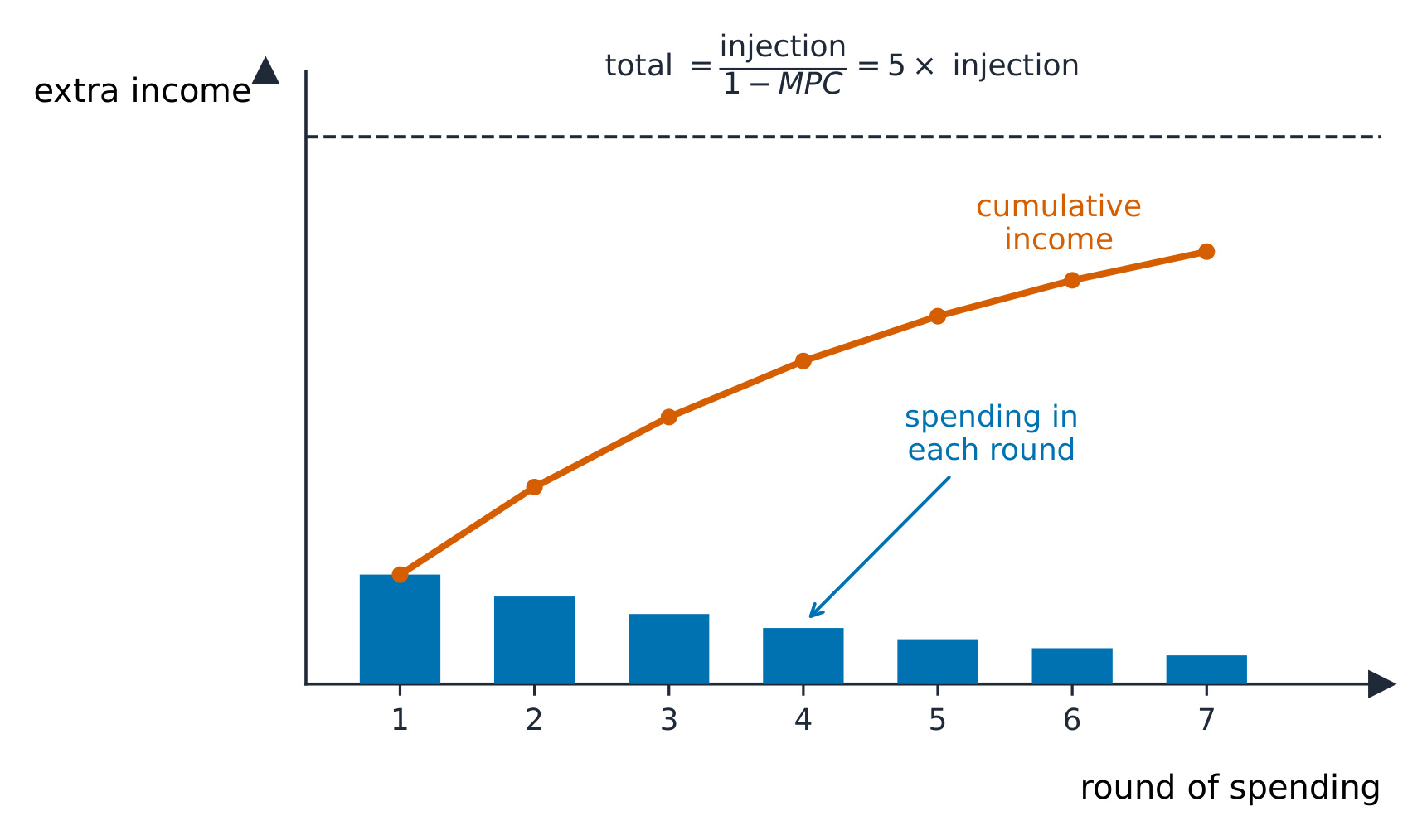
A change in spending sets off further rounds of spending, so the final change in GDP is larger than the initial change – the multiplier effect 乘数效应. It depends on the marginal propensity to consume 边际消费倾向 (MPC), the fraction of extra income that is spent (the rest is the marginal propensity to save 边际储蓄倾向, MPS, with $MPC+MPS=1$):

$$\text{spending multiplier}=\frac{1}{1-MPC}=\frac{1}{MPS}.$$

A tax cut works through the multiplier too, but more weakly, because part of the tax cut is saved:

$$\text{tax multiplier}=-\frac{MPC}{1-MPC}=-\frac{MPC}{MPS}.$$

The tax multiplier is smaller in size and negative (a tax cut raises GDP; a tax rise lowers it). Total change in GDP $=$ (multiplier) $\times$ (initial change).

Worked example. If $MPC=0.8$, the spending multiplier is $\dfrac{1}{1-0.8}=5$, so a $\$10$ billion rise in government spending lifts real GDP by $5\times\$10=\$50$ billion. The tax multiplier is $-\dfrac{0.8}{0.2}=-4$, so a $\$10$ billion tax cut raises GDP by only $\$40$ billion – weaker, because part of the tax cut is saved.

Exam skill: compute both multipliers from the MPC and find the resulting change in real GDP – an almost-guaranteed calculation.

日本語

支出乗数

支出の変化はさらなる支出の連鎖を引き起こすため、GDPの最終的な変化量は初期の変化量よりも大きい。これが乗数効果である。これは限界消費性向（MPC） に依存する。すなわち、追加所得のうち消費される割合であり、残りは限界貯蓄性向（MPS） として貯蓄される（$MPC+MPS=1$）。

1回のインジェクションが全体としてのより大きな所得増加に倍増する

$$\text{spending multiplier}=\frac{1}{1-MPC}=\frac{1}{MPS}.$$

減税も同様に乗数作用要通过するが、減税の一部が貯蓄されるため、その効果は相対的に弱い。

$$\text{tax multiplier}=-\frac{MPC}{1-MPC}=-\frac{MPC}{MPS}.$$

税乘数の絶対値は小さく、符号は負である（減税はGDPを増やし、増税はGDPを減らす）。GDPの変化量 = $=$（乘数） × $\times$（初期の変化量）。

** worked example.** $MPC=0.8$ の場合、支出乘数は $\dfrac{1}{1-0.8}=5$ となる。したがって、$\$10$ billion rise in government spending lifts real GDP by $5\times\$10=\$50$ billion. The tax multiplier is $-\dfrac{0.8}{0.2}=-4$, so a $\$10$ 億ドルの減税によってGDPはわずか $\$40$ 億ドルしか増加しない。減税の一部が貯蓄されるため、この効果は弱い。

** 試験対策：** MPCから両方の乘数を計算し、それに基づいて実質GDPの変化量を求める——これは出題頻度の高い計算問題である。

Explore · ⁨探索⁩

See the spending multiplier ripple out

A dollar of new spending becomes someone's income, part of which they spend again — so the total effect is a multiple of the first injection, set by the marginal propensity to consume (MPC).

3.3

Short-Run Aggregate Supply · ⁨短期総供給⁩

Syllabus · ⁨シラバス⁩

English

Enduring Understanding (MOD-2): Economists use the aggregate demand–aggregate supply model to represent the relationship between the price level and aggregate output in an economy and to illustrate how output, employment, and the price level respond to macroeconomic shocks.

Learning Objective MOD-2.C: a. Define (using graphs as appropriate) the short-run aggregate supply (SRAS) curve. b. Explain (using graphs as appropriate) the slope of the SRAS curve and its determinants.

MOD-2.C.1 The short-run aggregate supply (SRAS) curve describes the relationship between the price level and the quantity of goods and services supplied in an economy.
MOD-2.C.2 The SRAS curve is upward-sloping because of sticky wages and prices. [See EK MOD-2.E.1]
MOD-2.C.3 Any factor that causes production costs to change, such as a change in inflationary expectations, will cause the SRAS curve to shift.

Learning Objective MOD-2.D: Explain (using graphs as appropriate) how movement along the SRAS curve implies a relationship between the price level (and inflation) and unemployment.

MOD-2.D.1 Moving along the SRAS curve, an increase in the price level is associated with an increase in output, which means employment must correspondingly rise. With the labor force held constant, unemployment will fall. So, there is a short-run trade-off between inflation and unemployment. [See EK MOD-3.A.1]

日本語

持続的認識（MOD-2）： 経済学者は、価格水準と経済内の総生産量の関係を表現し、マクロ経済ショックに対する生産量、雇用、および価格水準の反応を示すために、総需要・総供給モデルを使用する。

学習目標 MOD-2.C: a. 短期総供給（SRAS）曲線を定義せよ（必要な場合は図を用いる）。 b. SRAS曲線の傾きとその決定要因を説明せよ（必要な場合は図を用いる）。

MOD-2.C.1 短期総供給（SRAS）曲線は、価格水準と経済内で供給される財・サービスの数量との関係を表す。
MOD-2.C.2 SRAS曲線が右上がりとなるのは、賃金や価格の粘着性のためである。[EK MOD-2.E.1参照]
MOD-2.C.3 インフレ期待の変化など、生産コストを変化させる要因があれば、SRAS曲線はシフトする。

学習目標 MOD-2.D: 短期総供給曲線上の移動が、価格水準（およびインフレ）と失業率との関係を示していることを説明せよ（必要な場合は図を用いる）。

MOD-2.D.1 SRAS曲線上を移動する場合、価格水準の上昇は生産量の増加に伴い、雇用も同様に増加しなければならない。労働力が一定であれば、失業率は低下する。したがって、インフレと失業の間には短期間のトレードオフがある。[EK MOD-3.A.1参照]

Source: College Board AP Course and Exam Description · ⁨出典: College Board AP コースおよび試験説明書⁩

English

Short-run aggregate supply (SRAS) 短期总供给 slopes upward: in the short run some input prices (especially nominal wages 名义工资) are sticky 粘性, so a higher output price level widens profit margins and firms produce more. SRAS shifts with input prices, productivity, taxes/subsidies on producers, and supply shocks (e.g. an oil-price change). A rise in input costs shifts SRAS left.

日本語

発電所および工業施設：短期総供給は生産コストに依存する

短期総供給（SRAS） は右上がりである。短期間では一部の投入財価格（特に名目賃金）が硬直的であるため、生産物価格水準の上昇は利益マージンを拡大させ、企業はより多くの生産を行う。SRASは投入財価格、生産性、生産者に対する税・補助金、そしてサプライ・ショック（石油価格の変動など）の変化に伴ってシフトする。投入コストの上昇はSRASを左へシフトさせる。

3.4

Long-Run Aggregate Supply · ⁨長期総供給⁩

Syllabus · ⁨シラバス⁩

English

Enduring Understanding (MOD-2): Economists use the aggregate demand–aggregate supply model to represent the relationship between the price level and aggregate output in an economy and to illustrate how output, employment, and the price level respond to macroeconomic shocks.

Learning Objective MOD-2.E: Define (using graphs as appropriate) the short run and the long run.

MOD-2.E.1 In the long run all prices and wages are fully flexible, while in the short run some input prices are fixed. A consequence of flexible long-run prices and wages is the lack of a long-run trade-off between inflation and unemployment.

Learning Objective MOD-2.F: Define (using graphs as appropriate) the long-run aggregate supply (LRAS) curve.

MOD-2.F.1 The LRAS curve corresponds to the production possibilities curve (PPC) because they both represent maximum sustainable capacity. Maximum sustainable capacity is the total output an economic system will produce over a set period of time if all resources are fully employed. [See LO MOD-2.I]
MOD-2.F.2 The LRAS curve is vertical at the full-employment level of output because in the long run wages and prices fully adjust.

日本語

持続的認識（MOD-2）： 経済学者は、価格水準と経済内の総生産量の関係を表現し、マクロ経済ショックに対する生産量、雇用、および価格水準の反応を示すために、総需要・総供給モデルを使用する。

学習目標 MOD-2.E: 短期と長期を定義せよ（必要な場合は図を用いる）。

MOD-2.E.1 長期ではすべての価格と賃金は完全に柔軟であるのに対し、短期では一部の投入品価格は固定されている。長期における価格と賃金の柔軟性の結果として、インフレと失業の間の長期のトレードオフは存在しない。

学習目標 MOD-2.F: 長期総供給（LRAS）曲線を定義せよ（必要な場合は図を用いる）。

MOD-2.F.1 LRAS曲線は生産可能性曲線（PPC）に対応する。なぜなら、両者は最大持続可能生産能力を表すからである。最大持続可能生産能力とは、全資源が完全に雇用された場合、経済システムが一定期間中に生産する総生産量である。[LO MOD-2.I参照]
MOD-2.F.2 LRAS曲線は完全雇用の生産量水準で垂直である。なぜなら、長期では賃金と価格が完全に調整されるからである。

Source: College Board AP Course and Exam Description · ⁨出典: College Board AP コースおよび試験説明書⁩

English

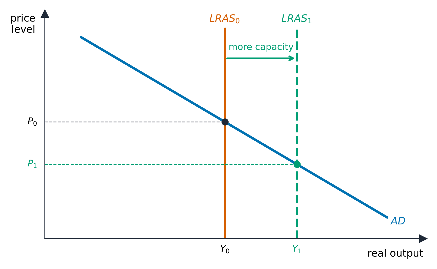
Long-run aggregate supply (LRAS) 长期总供给 is vertical at the economy's full-employment (potential) output 潜在产出 $Y_f$. In the long run all prices and wages are fully flexible (only in the short run are some input prices fixed), so output depends only on real factors – resources, technology, institutions – not the price level. LRAS shifts only with economic growth (more or better resources). LRAS corresponds to the production possibilities curve (PPC) 生产可能性曲线: both mark the economy's maximum sustainable capacity, so an outward LRAS shift and an outward PPC shift are the same event drawn two ways. The vertical LRAS is why, in the long run, demand policy changes prices, not output.

日本語

長期総供給（LRAS） は経済の完全雇用（潜在）産出量 $Y_f$ において垂直である。長期的にはすべての価格と賃金は完全に柔軟的である（投入財価格が固定されるのは短期的に過ぎない）。したがって、産出量は資源、技術、制度といった実質的要因にのみ依存し、物価水準には依存しない。LRASは経済成長（資源の増加や品質向上）によってのみシフトする。LRASは生産可能性曲線（PPC） と対応しており、どちらも経済の最大持続可能能力を示している。したがって、LRASの右方シフトとPPCの外方シフトは、同じ出来事を異なる角度から描いたものに他ならない。LRASが垂直であることが、長期的には需要政策が物価を変化させ、産出量には影響を与えない理由である。

供給側政策が長期総供給を右方へシフトさせる：産出量の増加と物価の低下

3.5

Equilibrium in the AD-AS Model · ⁨AD-ASモデルにおける均衡点⁩

Syllabus · ⁨シラバス⁩

English

Enduring Understanding (MOD-2): Economists use the aggregate demand–aggregate supply model to represent the relationship between the price level and aggregate output in an economy and to illustrate how output, employment, and the price level respond to macroeconomic shocks.

Learning Objective MOD-2.G: Explain (using graphs as appropriate) the short-run and long-run equilibrium price level and output level.

MOD-2.G.1 Short-run equilibrium occurs when the aggregate quantity of output demanded and the aggregate quantity of output supplied are equal—i.e., at the intersection of the AD and SRAS curves.
MOD-2.G.2 Long-run equilibrium occurs when the AD and SRAS curves intersect on the LRAS—i.e., at the full-employment level of real output.
MOD-2.G.3 The short-run equilibrium output can be at the full-employment level of output, above it, or below it, creating positive (i.e., inflationary) or negative (i.e., recessionary) output gaps.

日本語

持続的認識（MOD-2）： 経済学者は、価格水準と経済内の総生産量の関係を表現し、マクロ経済ショックに対する生産量、雇用、および価格水準の反応を示すために、総需要・総供給モデルを使用する。

学習目標 MOD-2.G: 短期および長期の均衡価格水準と生産量水準を説明せよ（必要な場合は図を用いる）。

MOD-2.G.1 短期均衡は、総需要される生産量の総計と総供給される生産量の総計が等しいときに生じる。すなわち、AD曲線とSRAS曲線の交点において生じる。
MOD-2.G.2 長期均衡は、AD曲線とSRAS曲線がLRAS上で交差するときに生じる。すなわち、実質生産量の完全雇用水準において生じる。
MOD-2.G.3 短期均衡での生産量は、完全雇用の生産量水準にある也可以是、それより高い也可以是、あるいは低い也可以是。これにより、正（インフレary）または負（景気後退ary）の生産ギャップが生じる。

Source: College Board AP Course and Exam Description · ⁨出典: College Board AP コースおよび試験説明書⁩

English

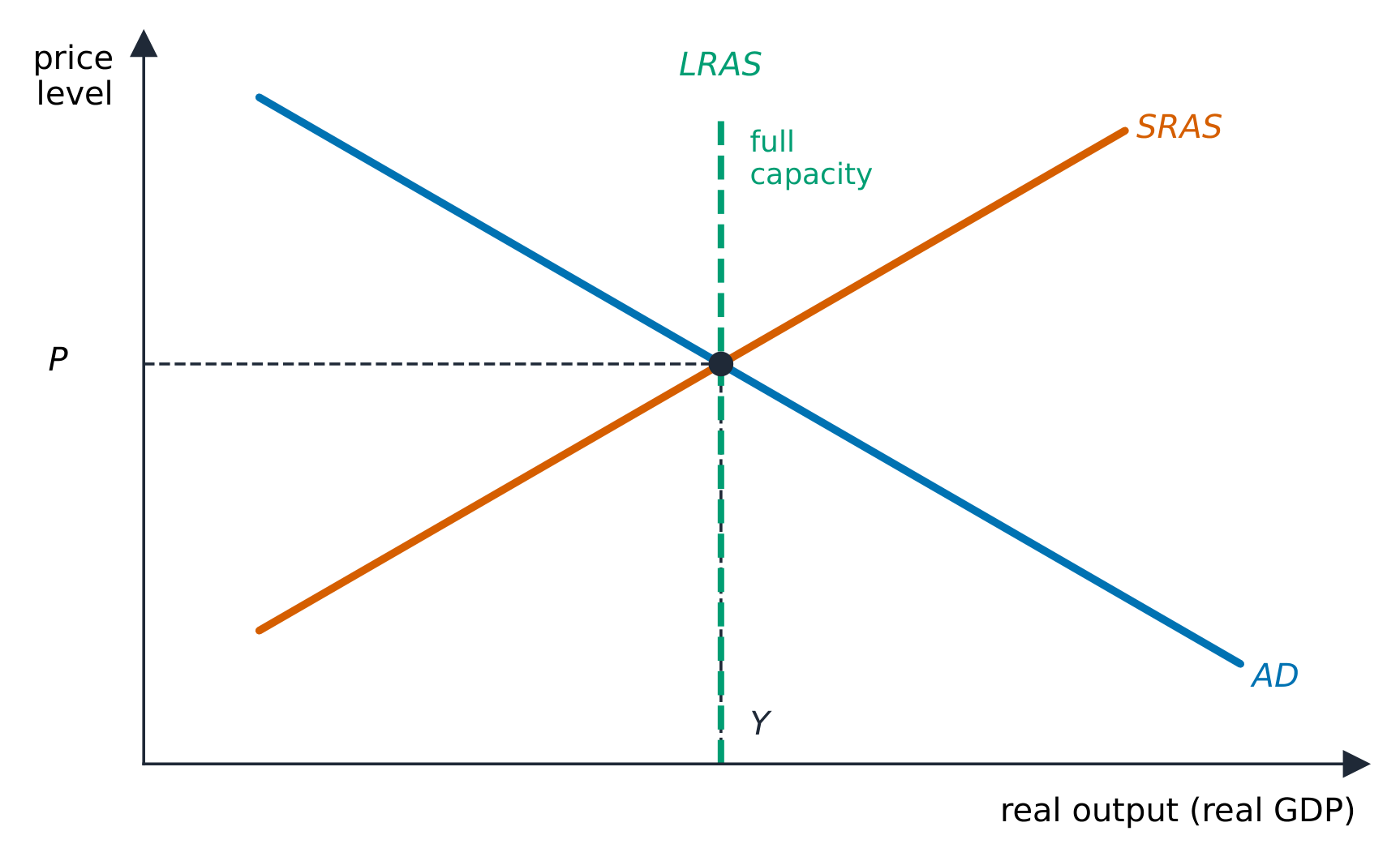
The economy settles where AD meets SRAS, fixing the equilibrium price level and real GDP. Comparing that output to $Y_f$ (the LRAS line) gives the economy's state:

output $: a recessionary gap 衰退缺口 (cyclical unemployment),
output $>Y_f$: an inflationary gap 通胀缺口 (overheating),
output $=Y_f$: long-run equilibrium.

日本語

経済はADとSRASが交差する地点で安定し、均衡物価水準と実質GDPが決定される。この産出量を $Y_f$ （LRASのライン）と比較することで、経済の状態が判別できる。

総需要と総供給が交差するマクロ経済の均衡点

産出量が $ ：景気後退ギャップ（循環的失業）
産出量が $>Y_f$ ：インフレギャップ（過熱）
産出量が $=Y_f$ ：長期均衡。

Explore · ⁨探索⁩

Find equilibrium in the AD-AS model

Aggregate demand and aggregate supply cross at the economy's price level and real GDP. A demand or supply shock shifts a curve and moves the whole economy's output and prices.

3.6

Short-Run Changes: Demand and Supply Shocks · ⁨短期変動：需要および供給ショック⁩

Syllabus · ⁨シラバス⁩

English

Enduring Understanding (MOD-2): Economists use the aggregate demand–aggregate supply model to represent the relationship between the price level and aggregate output in an economy and to illustrate how output, employment, and the price level respond to macroeconomic shocks.

Learning Objective MOD-2.H: Explain (using graphs as appropriate) the response of output, employment, and the price level to an aggregate demand or aggregate supply shock in the short run.

MOD-2.H.1 A positive (negative) shock in AD causes output, employment, and the price level to rise (fall) in the short run.
MOD-2.H.2 A positive (negative) shock in SRAS causes output and employment to rise (fall) and the price level to fall (rise) in the short run.
MOD-2.H.3 Inflation can be caused by changes in aggregate demand (demand-pull) or aggregate supply (cost-push).

日本語

持続的認識（MOD-2）： 経済学者は、価格水準と経済内の総生産量の関係を表現し、マクロ経済ショックに対する生産量、雇用、および価格水準の反応を示すために、総需要・総供給モデルを使用する。

学習目標 MOD-2.H: 短期における総需要または総供給ショックに対する、生産量、雇用、および価格水準の反応を説明せよ（必要な場合は図を用いる）。

MOD-2.H.1 ADに正（負）のショックが生じると、短期において生産量、雇用、物価水準が上昇（低下）する。
MOD-2.H.2 SRASに正（負）のショックが生じると、短期において生産量と雇用が上昇（低下）し、物価水準が低下（上昇）する。
MOD-2.H.3 インフレは総需要の変化（需要牽引型）または総供給の変化（コストプッシュ型）によって引き起こされることがある。

Source: College Board AP Course and Exam Description · ⁨出典: College Board AP コースおよび試験説明書⁩

English

A demand shock shifts AD: a positive one (more spending) raises both price level and output (and lowers unemployment); a negative one lowers both.
A supply shock shifts SRAS: a negative one (higher input costs) raises the price level and lowers output at once – stagflation 滞胀 – the hardest case for policymakers, because fixing one worsens the other.

日本語

需要ショックはADをシフトさせる。好意的なショック（支出増加）は物価水準と産出量をともに引き上げ（失業率は低下）、不況なショックは両方を低下させる。
供給ショックはSRASをシフトさせる。不況なショック（投入コストの上昇）は、物価水準を上げると同時に産出量を下げる——これがスタグフレーションである。政策立案者にとって最も困難なケースであり、一方を修正しようとすればもう一方が悪化するからだ。

3.7

Long-Run Self-Adjustment · ⁨長期の自己調整⁩

Syllabus · ⁨シラバス⁩

English

Enduring Understanding (MOD-2): Economists use the aggregate demand–aggregate supply model to represent the relationship between the price level and aggregate output in an economy and to illustrate how output, employment, and the price level respond to macroeconomic shocks.

Learning Objective MOD-2.I: Explain (using graphs as appropriate) the response of output, employment, and the price level to an aggregate demand or aggregate supply shock in the long run.

MOD-2.I.1 In the long run, in the absence of government policy actions, flexible wages and prices will adjust to restore full employment and unemployment will revert to its natural rate after a shock to aggregate demand or short-run aggregate supply. [See EK MEA-1.E.2]
MOD-2.I.2 Shifts in the long-run aggregate supply curve indicate changes in the full-employment level of output and economic growth.

日本語

持続的認識（MOD-2）： 経済学者は、価格水準と経済内の総生産量の関係を表現し、マクロ経済ショックに対する生産量、雇用、および価格水準の反応を示すために、総需要・総供給モデルを使用する。

学習目標 MOD-2.I: 総需要または総供給のショックに対する、長期における生産量、雇用、および物価水準の反応を説明する（必要に応じてグラフを用いる）。

MOD-2.I.1 長期において、政府による政策介入がない場合、柔軟な賃金と価格が調整され、總需要または短期総供給へのショック後には完全雇用の状態に戻り、失業率は自然率に戻る。[EK MEA-1.E.2 を参照]
MOD-2.I.2 長期総供給曲線のシフトは、完全雇用量の水準の変化や経済成長を示す。

Source: College Board AP Course and Exam Description · ⁨出典: College Board AP コースおよび試験説明書⁩

English

Left alone, the economy self-corrects through flexible wages:

In a recessionary gap, high unemployment eventually pushes nominal wages down, shifting SRAS right until output returns to $Y_f$ at a lower price level.
In an inflationary gap, labor shortages push wages up, shifting SRAS left back to $Y_f$ at a higher price level.

The debate over how fast this happens is the case for (or against) active policy: self-adjustment is slow and painful, which is the argument for intervening.

日本語

何もしなければ、経済は柔軟な賃金を通じて自己修正する。

景気後退ギャップにおいては、高い失業率が最終的に名目賃金を低下させ、SRASを右方へシフトさせ、物価水準が下がる中で産出量が $Y_f$ に戻る。
インフレギャップにおいては、労働不足が賃金を上昇させ、SRASを左方へシフトさせ、物価水準が上がる中で産出量が $Y_f$ に戻る。

この調整がどの程度速いのかに関する議論は、積極的な政策支援の有無の論争につながる。自己調整は遅く痛みを伴うため、介入すべきだという主張の根拠となる。

3.8

Fiscal Policy · ⁨財政政策⁩

Syllabus · ⁨シラバス⁩

English

Enduring Understanding (POL-1): Fiscal and monetary policy have short-run effects on macroeconomic outcomes.

Learning Objective POL-1.A: a. Define fiscal policy and related terms. b. Explain (using graphs as appropriate) the short-run effects of a fiscal policy action. c. Calculate the short-run effects of a fiscal policy action.

POL-1.A.1 Governments implement fiscal policies to achieve macroeconomic goals, such as full employment.
POL-1.A.2 The tools of fiscal policy are government spending and taxes/transfers.
POL-1.A.3 Changes in government spending affect aggregate demand directly, and changes in taxes/transfers affect aggregate demand indirectly.
POL-1.A.4 The government spending multiplier is greater than the tax multiplier.
POL-1.A.5 Expansionary or contractionary fiscal policies are used to restore full employment when the economy is in a negative (i.e., recessionary) or positive (i.e., inflationary) output gap.
POL-1.A.6 Fiscal policy can influence aggregate demand, real output, and the price level. [See also EK MKT-5.E.2 for the effect on exchange rates.]
POL-1.A.7 The AD–AS model is used to demonstrate the short-run effects of fiscal policy.

Learning Objective POL-1.B: Define why there are lags to discretionary fiscal policy.

POL-1.B.1 In reality, there are lags to discretionary fiscal policy because of factors such as the time it takes to decide on and implement a policy action.

日本語

永続的理解 (POL-1): 財政政策と金融政策は、マクロ経済の成果に短期的な影響を与える。

学習目標 POL-1.A: a. 財政政策および関連用語を定義する。 b. 財政政策の実施がもたらす短期的な影響を説明する（必要に応じてグラフを用いる）。 c. 財政政策の実施がもたらす短期的な影響を計算する。

POL-1.A.1 政府は完全雇用などのマクロ経済目標を達成するために財政政策を実施する。
POL-1.A.2 財政政策の手段は、政府支出と税金・給付である。
POL-1.A.3 政府支出の変化は総需要に直接的に影響を与え、税金/給付の変化は総需要に間接的に影響を与える。
POL-1.A.4 政府支出乗数は税乘数より大きい。
POL-1.A.5 景気がマイナス（＝景気後退ギャップ）またはプラス（＝インフレギャップ）の状況にある際、完全雇用の回復のために拡張的または緊縮的な財政政策が用いられる。
POL-1.A.6 財政政策は総需要、実質生産量、および物価水準に影響を与えることができる。[為替レートへの影響については EK MKT-5.E.2 も参照]。
POL-1.A.7 AD–ASモデルは、財政政策の短期的な効果を示すために用いられる。

学習目標 POL-1.B: 裁量的財政政策に遅延が生じる理由を定義する。

POL-1.B.1 現実において、裁量的財政政策には遅延が生じる。これは、政策の実施に決定を下すのに時間がかかることなどの要因による。

Source: College Board AP Course and Exam Description · ⁨出典: College Board AP コースおよび試験説明書⁩

English

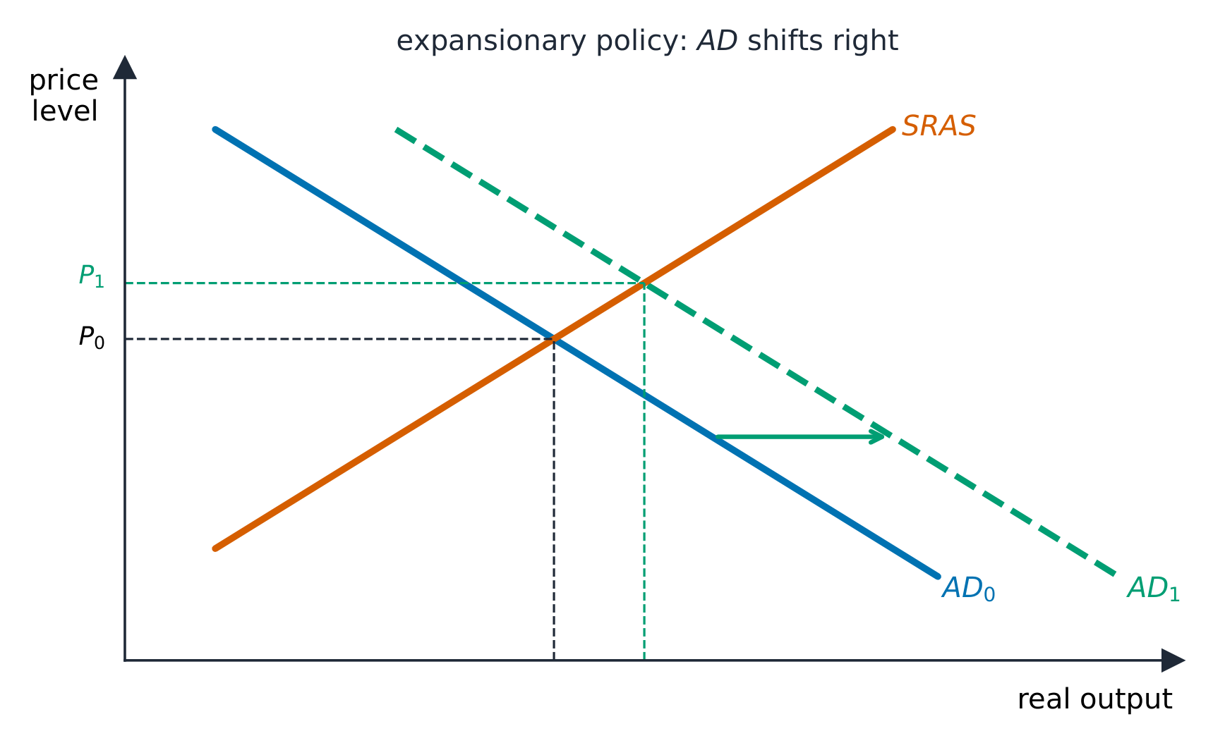
Fiscal policy 财政政策 is the government's use of spending and taxes to shift AD:

Expansionary 扩张性 (more spending or lower taxes) shifts AD right to close a recessionary gap.
Contractionary 紧缩性 (less spending or higher taxes) shifts AD left to close an inflationary gap.

Size the policy with the multipliers: to close a gap of a given size, the required change in spending is (gap) $\div$ (spending multiplier). Limits include time lags, crowding out (below), and political difficulty.

Worked example. An economy has a $\$100$ billion recessionary gap and $MPC=0.75$ (spending multiplier $=\dfrac{1}{0.25}=4$). To close it, the government must raise spending by $\dfrac{\$100\text{ billion}}{4}=\$25$ billion. Using a tax cut instead (tax multiplier $-3$) would require a larger $\dfrac{100}{3}\approx\$33$ billion cut.

Exam skill: you must draw the correctly labeled AD-AS graph, identify the gap, prescribe the right fiscal action and its direction, and often calculate the exact spending or tax change needed.

日本語

財政政策とは、政府が支出と税を用いてADをシフトさせることである。

拡張的財政政策がADを右方へシフトさせ、産出量と物価を引き上げる

拡張的（支出増加または減税）はADを右方へシフトさせ、景気後退ギャップを埋める。
緊縮的（支出削減または増税）はADを左方へシフトさせ、インフレギャップを埋める。

乗数を用いて政策の規模を決定する：特定のサイズのギャップを埋めるために必要な支出の変化量は (ギャップ) $\div$ (支出乗数) である。限界にはタイムラグ、クラウドアウト効果（以下参照）、政治的な難しさがある。

** worked example.** 経済の$\$100$ billion recessionary gap and $MPC=0.75$ (spending multiplier $=\dfrac{1}{0.25}=4$). To close it, the government must raise spending by $\dfrac{\$100\text{ billion}}{4}=\$25$ billion. Using a tax cut instead (tax multiplier $-3$) would require a larger $\dfrac{100}{3}\approx\$33$ billion cut.

** Exam skill:** 正しくラベル付けされたAD-ASグラフを描き、ギャップを特定し、適切な財政政策とその方向性を指定し、必要な支出や税制変更の正確な額を計算することが求められます。

Vocabulary · ⁨語彙⁩ Train · ⁨練習する⁩

English	日本語
Aggregate demand (AD)/ˈæɡrɪɡeɪt dɪˈmænd/	総需要（AD）
price level/praɪs ˈlevl/	物価水準である
wealth effect/welθ ɪˈfekt/	富の効果
interest-rate effect/ˈɪntrest reɪt ɪˈfekt/	利子率効果
multiplier effect/ˌmʌltɪˈplaɪə ɪˈfekt/	乗数効果
marginal propensity to consume/ˈmɑːdʒɪnl prəˈpensɪti tə kənˈsjuːm/	限界消費性向
marginal propensity to save/ˈmɑːdʒɪnl prəˈpensɪti tə seɪv/	限界貯蓄性向
Short-run aggregate supply (SRAS)/ʃɔːt rʌn ˈæɡrɪɡeɪt səˈplaɪ/	短期総供給曲線（SRAS）
nominal wages/ˈnɒmɪnl ˈweɪdʒɪz/	名目賃金
sticky/ˈstɪki/	粘着性だからである
Long-run aggregate supply (LRAS)/lɒŋ rʌn ˈæɡrɪɡeɪt səˈplaɪ/	長期総供給曲線（LRAS）
full-employment (potential) output/fʊl emˈplɔɪmənt ˈaʊtpʊt/	完全雇用産出量（潜在成長率）
production possibilities curve (PPC)/prəˈdʌkʃn ˌpɒsəˈbɪlɪtiz kɜːv/	生産可能性 Frontier（PPF）
recessionary gap/rɪˈseʃənəri ɡæp/	リセッション・ギャップが生じる
inflationary gap/ɪnˈfleɪʃənəri ɡæp/	インフレーション・ギャップが生じる
stagflation/stæɡˈfleɪʃn/	スタグフレーション
Fiscal policy/ˈfɪskl ˈpɒlɪsi/	財政政策
Expansionary/ekˈspænʃənəri/	拡張的
Contractionary/kənˈtrækʃənəri/	緊縮的

3.9

Automatic Stabilizers

Syllabus · ⁨シラバス⁩

English

Enduring Understanding (POL-1): Fiscal and monetary policy have short-run effects on macroeconomic outcomes.

Learning Objective POL-1.C: a. Define automatic stabilizers. b. Explain how automatic stabilizers moderate business cycles.

POL-1.C.1 Automatic stabilizers support the economy during recessions and help prevent the economy from being overheated during expansionary periods.
POL-1.C.2 Tax revenues decrease automatically as GDP falls, preventing consumption and the economy from falling further.
POL-1.C.3 Tax revenues increase automatically as GDP rises, slowing consumption and preventing the economy from overheating.
POL-1.C.4 Government policies, institutions, or agencies may also have social service programs whose transfer payments act as automatic stabilizers.

日本語

永続的理解 (POL-1): 財政政策と金融政策は、マクロ経済の成果に短期的な影響を与える。

学習目標 POL-1.C: a. 自動安定装置を定義する。 b. 自動安定装置が景気循環を緩和する仕組みを説明する。

POL-1.C.1 自動安定装置は景気後退時に経済を支え、拡張期に経済が過熱するのを防ぐ役割を果たす。
POL-1.C.2 GDPが下落すると税収が自動的に減少し、消費や経済のさらなる低下を防ぐ。
POL-1.C.3 GDPが上昇すると税収が自動的に増加し、消費を抑制して経済の過熱を防ぐ。
POL-1.C.4 政府の政策、制度、機関によっては、社会福祉プログラムを有しており、その給付金が自動安定装置として機能することがある。

Source: College Board AP Course and Exam Description · ⁨出典: College Board AP コースおよび試験説明書⁩

English

Automatic stabilizers 自动稳定器 are features that dampen the cycle without new legislation. In a downturn, progressive taxes collect less and transfer payments (unemployment benefits, welfare) rise automatically – cushioning incomes and spending; in a boom they do the reverse. They soften the cycle and act instantly, avoiding the lags of discretionary 相机抉择 policy.

日本語

** Automatic stabilizers** は、新たな立法なしに景気循環を緩和する機能です。不況期には、累進税制による徴収額が減り、給付金（失業保険、生活保護）が自動的に増加して所得と消費を支えます。好況期にはその逆が行われます。これらは景気循環を緩やかにし、裁量型政策の遅れを回避します。

Vocabulary · ⁨語彙⁩ Train · ⁨練習する⁩

English	日本語
Automatic stabilizers/ˌɔːtəˈmætɪk ˈsteɪbəlaɪzəz/	自動安定装置
discretionary/dɪˈskreʃənəri/	裁量的

3.9

Exam tips · ⁨試験対策⁩

English

Aggregate demand slopes down for the wealth, interest-rate, and net-export effects; it shifts when $C$, $I$, $G$, or $X_n$ changes.
Compute the spending multiplier $\tfrac{1}{1-MPC}$ and the smaller, negative tax multiplier $-\tfrac{MPC}{1-MPC}$.
Draw a correctly labeled AD–AS graph, identify a recessionary or inflationary gap, and prescribe the right fiscal action.
Short-run AS slopes up (sticky wages); long-run AS is vertical at full-employment output.
Size a policy with the multipliers: required spending = gap ÷ spending multiplier.

日本語

総需要曲線は、財 Wealth効果、利子率効果、純輸出効果により右下がりです。** $C$, $I$, $G$, $X_n$ ** が変化するとシフトします。
支出乗数 $\tfrac{1}{1-MPC}$ と、より小さい負の 税制乗数 $-\tfrac{MPC}{1-MPC}$ を計算します。
正しくラベル付けされたAD–ASグラフを描き、リセッション・ギャップまたはインフレーション・ギャップを特定し、適切な財政政策を指定します。
短期AS曲線は右肩上がり（賃金の粘着性のため）、長期AS曲線は完全雇用産出量において垂直です。
乗数を用いて政策の規模を決定します：必要な支出＝ギャップ ÷ 支出乗数。

Interactive lessons on this topic · ⁨このトピックのインタラクティブ授業⁩

Work through it step by step, with instant-check exercises. · ⁨一歩ずつ進め、即時チェック付きの問題で学習します。⁩

Past Papers · ⁨過去問⁩

More topics in AP Macroeconomics · ⁨AP マクロ経済学⁩ · ⁨AP Macroeconomics · ⁨AP マクロ経済学⁩ の他のトピック⁩