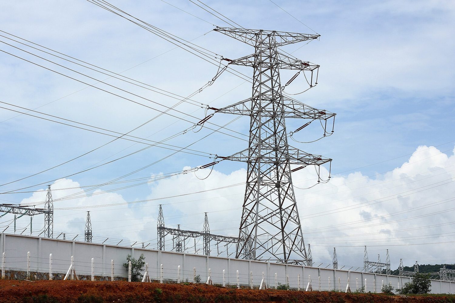
Look at these numbers. A small battery says one point five volts. A car battery says twelve. A high-voltage transmission line carries four hundred thousand. A…
English narration · English + 中文 subtitles burned in · קריאת קול באנגלית · תרגום אנגלי + סינית שרוף בתוך הסרטון
9.1
Electric Potential Energy · אנרגיה פוטנציאלית חשמלית
Syllabus · סיילבוס
English
Learning Objective 9.1.A: Describe the electric potential energy of a system.
9.1.A.1 The electric potential energy of a system of two point charges equals the amount of work required for an external force to bring the point charges to their current positions from infinitely far away.
9.1.A.2 The general form for the electric potential energy between two charged objects is given by the equation
9.1.A.3 The total electric potential energy of a system can be determined by finding the sum of the electric potential energies of the individual interactions between each pair of charged objects in the system.
עברית
מטרת הלמידה 9.1.A: לתאר את האנרגיה הפוטנציאלית חשמלית של מערכת.
9.1.A.1 האנרגיה הפוטנציאלית חשמלית של מערכת של שני מטעני נקודה שווה לכמות העבודה הנדרשת מכוח חיצוני להביא את מטעני הנקודה למיקומם הנוכחי מרחק אינסופי.
9.1.A.2 הצורה הכללית עבור האנרגיה הפוטנציאלית חשמלית בין שני גופים טעונים נתונה על ידי המשוואה
9.1.A.3 את האנרגיה הפוטנציאלית החשמלית הכוללת של מערכת ניתן לקבוע על ידי מציאת הסכום של האנרגיות הפוטנציאליות החשמליות של האינטראקציות הבודדות בין כל זוג של גופים טעונים במערכת.
Source: College Board AP Course and Exam Description · מקור: תיאור הקורס והמבחן של College Board AP
English
When you push two like charges together, you do work 功 against the electric force. That work is stored by the pair as electric potential energy 电势能:
$U_E$ is defined as the work an external force must do to bring the charges from infinitely far away to a distance $r$ apart. The signs carry the physics:
Like charges:$U_E>0$. An outside push was needed to bring them together. If released, they fly apart, and the stored energy becomes kinetic energy 动能.
Opposite charges:$U_E<0$. The pair is bound. You must supply $|U_E|$ of work to pull them apart to infinity.
The electric force is a conservative force 保守力: the work it does depends only on the start and end points, not the path, and equals $-\Delta U_E$.
For a system 系统 of several charges, add the potential energy of every distinct pair:
Worked example. Three $+2.0\ \mu\text{C}$ charges sit at the corners of an equilateral triangle with sides $0.30\ \text{m}$. Each pair stores $U=\dfrac{kq^2}{r}=\dfrac{(9.0\times10^{9})(2.0\times10^{-6})^2}{0.30}=0.12\ \text{J}$. There are three pairs, so $U_{\text{total}}=3\times0.12\ \text{J}=0.36\ \text{J}$. This is the work needed to assemble the triangle from infinity – and the kinetic energy the charges would share if all three were released.
עברית
כשדוחפים שני מטענים דומים יחד, אתם מבצעים עבודה נגד הכוח החשמלי. עבודה זו מאוחסנת על ידי הזוג כ-אנרגיה פוטנציאלית חשמלית:
דוגמה מפורטת. שלושה מטענים $+2.0\ \mu\text{C}$ נמצאים בקודקודי משולש שווה צלעות עם צלעות $0.30\ \text{m}$. כל זוג מאחסן $U=\dfrac{kq^2}{r}=\dfrac{(9.0\times10^{9})(2.0\times10^{-6})^2}{0.30}=0.12\ \text{J}$. ישנם שלושה זוגות, ולכן $U_{\text{total}}=3\times0.12\ \text{J}=0.36\ \text{J}$. זהו העבודה הנדרשת להרכבת המשולש מאינסוף – ואנרגיית הקינט שהמטענים היו חולקים אילו שחררו את כולם.
9.2
Electric Potential · פוטנציאל חשמלי
Syllabus · סיילבוס
English
Learning Objective 9.2.A: Describe the electric potential due to a configuration of charged objects.
9.2.A.1 Electric potential describes the electric potential energy per unit charge at a point in space.
9.2.A.2 Expressions for the electric potential of charge distributions can be found using integration and the principle of superposition.
9.2.A.2.i The electric potential for single point charge is
Equation:$V = \dfrac{q}{4\pi\varepsilon_0 r}$.
9.2.A.2.ii The electric potential due to multiple point charges can be determined by the principle of scalar superposition of the electric potential due to each of the point charges.
9.2.A.3 The electric potential difference between two points is the change in electric potential energy per unit charge when a test charge is moved between the two points.
Equation:$\Delta V = \dfrac{\Delta U_E}{q}$
9.2.A.4 Electric potential difference may also result from chemical processes that cause positive and negative charges to separate, such as in a battery.
Boundary statement: AP Physics C: Electricity & Magnetism only expects students to use calculus to find the electric potential resulting from the following charge distributions and locations: an infinitely long, uniformly charged wire or cylinder at a distance from its central axis, a thin ring of charge at a location along the axis of the ring, a semicircular arc or part of a semicircular arc at its center, and a finite wire or line charge at a point collinear with the line charge or at a location along its perpendicular bisector.
Learning Objective 9.2.B: Describe the relationship between electric potential and electric field.
9.2.B.1 The value of an electric field component in any direction at a given location is equal to the negative of the spatial rate of change in electric potential at that location.
Equation:$E_x = -\dfrac{dV}{dx}$
9.2.B.2 The change in electric potential between two points can be determined by integrating the dot product of the electric field and the displacement along the path connecting the points.
Equation:$\Delta V = V_b - V_a = -\displaystyle\int_a^b \vec{E}\cdot d\vec{r}$
9.2.B.3 Electric field vector maps and equipotential lines are tools to describe the field produced by a charge or configuration of charges and can be used to predict the motion of charged objects in the field.
9.2.B.3.i Equipotential lines represent lines of equal electric potential. These lines are also referred to as isolines of electric potential.
9.2.B.3.ii Isolines are perpendicular to electric field vectors. An isoline map of electric potential can be constructed from an electric field vector map, and an electric field map may be constructed from an isoline map.
9.2.B.3.iii An electric field vector points in the direction of decreasing potential.
9.2.B.3.iv There is no component of an electric field along an isoline.
עברית
מטרת הלמידה 9.2.A: לתאר את הפוטנציאל החשמלי הנובע מסידור של גופים טעונים.
9.2.A.1 פוטנציאל חשמלי מתאר את האנרגיה הפוטנציאלית חשמלית ליחידת מטען בנקודה במרחב.
9.2.A.2 ביטויים לפוטנציאל חשמלי של חלוקות מטען יכולים להתקבל באמצעות אינטגרציה ועקרון ההיתכבות.
9.2.A.2.ii הפוטנציאל החשמלי הנובע ממספר מטענים נקודתיים ניתן לקביעה על פי עקרון הסופרפוזיציה הסקלרית של הפוטנציאל החשמלי הנובע מכל אחד מהמטענים הנקודתיים.
9.2.A.3 ההפרש בפוטנציאל החשמלי בין שני נקודות הוא השינוי באנרגיה הפוטנציאלית החשמלית ליחידת מטען כאשר מטען מבחון מוזז בין שתי הנקודות.
משוואה:$\Delta V = \dfrac{\Delta U_E}{q}$
9.2.A.4 הפרש בפוטנציאל חשמלי עשוי לנבוע גם מתהליכים כימיים הגורמים להפרדת מטענים חיוביים ושליליים, כגון בסוללה.
הצהרת גבול: AP Physics C: חשמל ומגנטיות מצפה רק משתמשים להשתמש בקalkulus כדי למצוא את הפוטנציאל החשמלי הנובע מהחלוקות המטען והמיקומים הבאים: חוט או צילינדר טעונים באופן אחיד ואינסופי ארוך במרחק מהציר המרכזי שלו, טבעת דקה טעונה במיקום לאורך ציר הטבעת, קשת חצי-מעגלית או חלק מקשת חצי-מעגלית במרכזה, וחוט סופי או מטען קווי בנקודה הקולינארית עם המטען הקווי או במיקום לאורך האנכי המוצא לו.
מטרות הלמידה 9.2.B: לתאר את הקשר בין פוטנציאל חשמלי לשדה חשמלי.
9.2.B.1 הערך של רכיב שדה חשמלי בכל כיוון במיקום נתון שווה למינוס הקצב המרחבי של השינוי בפוטנציאל החשמלי במיקום זה.
משוואה:$E_x = -\dfrac{dV}{dx}$
9.2.B.2 השינוי בפוטנציאל החשמלי בין שתי נקודות יכול לקביעה על ידי אינטגרציה של מכפלת הנקודתית של השדה החשמלי והתזחה לאורך המסלול המקשר בין הנקודות.
משוואה:$\Delta V = V_b - V_a = -\displaystyle\int_a^b \vec{E}\cdot d\vec{r}$
9.2.B.3 מפות וקטוריות של שדה חשמלי וקווי פוטנציאל שווה הן כלים לתאר את השדה הנוצר על ידי מטען או תצורת מטענים וניתן להשתמש בהם לחזות את התנועה של גופים טעונים בשדה.
9.2.B.3.i קווי פוטנציאל שווה מייצגים קווים בעלי פוטנציאל חשמלי שווה. קווים אלו מכונים לעיתים קרובות גם כקווי איזולין של פוטנציאל חשמלי.
9.2.B.3.ii קווי איזולין מאונכים לוקטורים של שדה חשמלי. ניתן לבנות מפת קווי איזולין של פוטנציאל חשמלי מתוך מפת וקטוריות של שדה חשמלי, ומפת שדה חשמלית עשויה להיות נבנית מתוך מפת קווי איזולין.
9.2.B.3.iii וקטור של שדה חשמלי מצביע בכיוון של ירידה בפוטנציאל.
9.2.B.3.iv אין רכיב של שדה חשמלא לאורך קו איזולין.
Source: College Board AP Course and Exam Description · מקור: תיאור הקורס והמבחן של College Board AP
English
Electric potential 电势 is electric potential energy per unit charge at a point in space. It is measured in volts ($1\ \text{V}=1\ \text{J/C}$):
Potential is a scalar 标量: it has a sign but no direction. This makes $V$ far easier to work with than the field $\vec{E}$. For several point charges 点电荷, use scalar superposition 叠加 – add the potentials with their signs:
Worked example. The potential $0.10\ \text{m}$ from a $+3.0\ \text{nC}$ point charge is $V=\dfrac{kq}{r}=\dfrac{9.0\times10^{9}(3.0\times10^{-9})}{0.10}=270\ \text{V}$. Now add a $-3.0\ \text{nC}$ charge $0.30\ \text{m}$ from the same point: it contributes $\dfrac{9.0\times10^{9}(-3.0\times10^{-9})}{0.30}=-90\ \text{V}$, so the total is $270-90=180\ \text{V}$. Just a signed sum – no vector components to resolve.
Continuous charge distributions
For a continuous charge distribution 连续电荷分布, cut it into small pieces $dq$, treat each piece as a point charge, and integrate 积分:
This is a scalar integral, so it is usually much easier than the field integral. AP expects you to handle four shapes with calculus: a thin ring (at a point on its axis), an arc (at its centre), a finite line or wire (collinear, or on its perpendicular bisector), and an infinitely long wire or cylinder (at a distance from its axis).
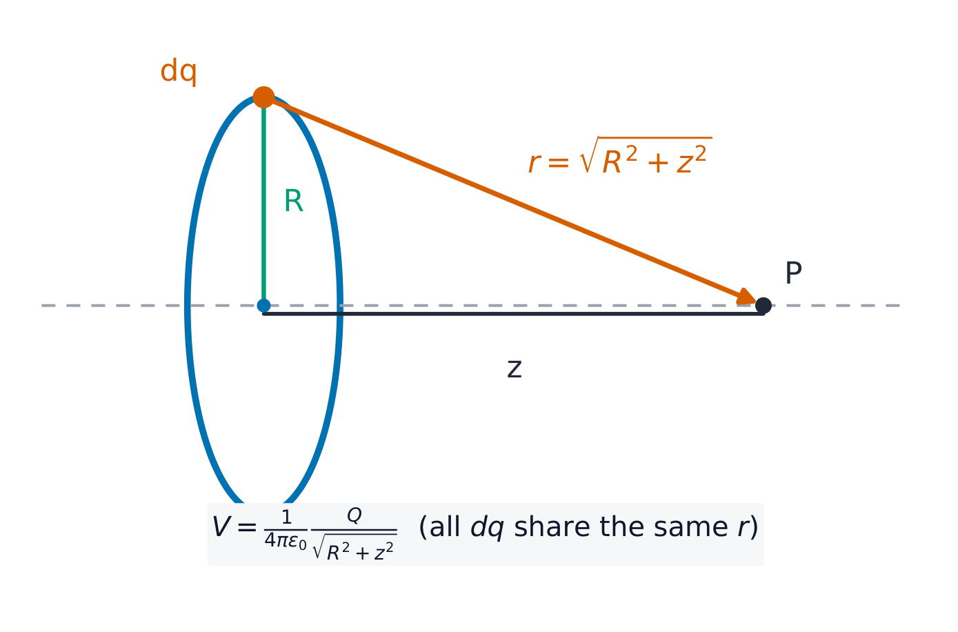
Worked example (ring of charge). A thin ring of radius $R$ carries total charge $Q$. For a point $P$ on the axis a distance $z$ from the centre, every element $dq$ sits at the same distance $r=\sqrt{R^2+z^2}$ from $P$. The distance is constant, so it comes out of the integral:
On an FRQ, say that $r$ is the same for every element – that statement is the marked step. The same idea gives $V=kQ/R$ at the centre of any arc, whatever its angle.
From potential to field
Potential and field contain the same information, linked by a derivative in each direction and by a path integral:
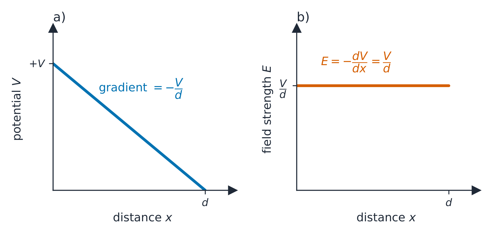
The field is the negative gradient 梯度 of the potential: $\vec{E}$ points from high potential to low potential, "downhill". Where $V$ changes quickly, the field is strong.
Worked example. Along the $x$-axis, $V(x)=3x^{2}-2x$ (volts, with $x$ in metres). Then $E_x=-\dfrac{dV}{dx}=2-6x\ \text{V/m}$. At $x=0.50\ \text{m}$, $E_x=-1.0\ \text{V/m}$: the field there points in the $-x$ direction.
The potential difference 电势差 between two points is the change in potential energy per unit charge moved between them: $\Delta V=\Delta U_E/q$. A battery makes a potential difference chemically: reactions inside separate positive from negative charge and hold the terminals a fixed $\Delta V$ apart.
Equipotential maps
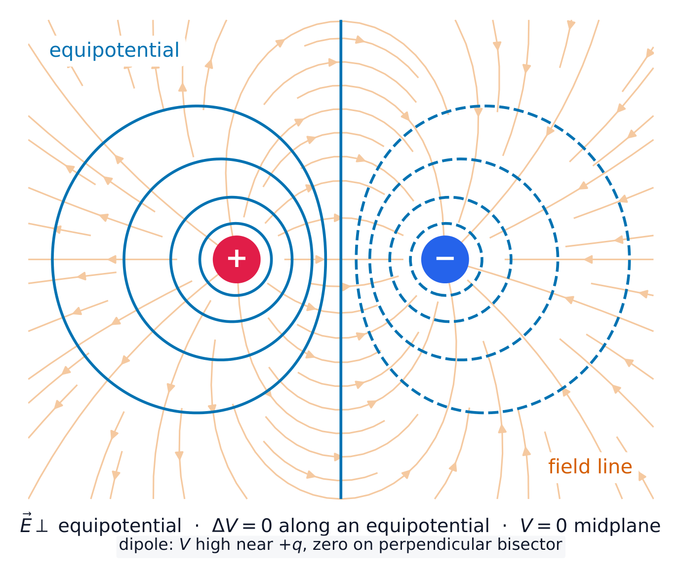
An equipotential 等势面 line (also called an isoline 等值线) joins points that share the same potential. Four rules let you read any map:
Isolines are perpendicular 垂直 to field lines 电场线 everywhere they cross.
$\vec{E}$ points from high $V$ to low $V$ – never along an isoline. Moving a charge along an isoline takes no work.
Closely spaced isolines mean a strong field: $E\approx-\Delta V/\Delta x$.
You can sketch the field map from an isoline map, and the isoline map from a field map.
Exam skill. Given a map with isolines every $10\ \text{V}$ spaced about $2\ \text{cm}$ apart, estimate $E\approx\dfrac{10}{0.02}=500\ \text{V/m}$, pointing from the higher-value line to the lower one. The work an external agent does moving a charge $q$ slowly from $A$ to $B$ is $W=q(V_B-V_A)$ – the path taken does not matter.
עברית
פוטנציאל חשמלי הוא אנרגיה פוטנציאלית חשמלית ליחידת מטען בנקודה במרחב. הוא נמדד בוולטים ($1\ \text{V}=1\ \text{J/C}$):
הפוטנציאל הוא סקלרי: יש לו סימן אך אין לו כיוון. הדבר הופך את $V$ לקל הרבה לעיבוד מאשר השדה $\vec{E}$. עבור מספר מטעני נקודה, השתמש ב-סיכום סקלרי – חבר את הפוטנציאלים עם הסימנים שלהם:
דוגמה מפורטת. הפוטנציאל $0.10\ \text{m}$ ממטען נקודה $+3.0\ \text{nC}$ הוא $V=\dfrac{kq}{r}=\dfrac{9.0\times10^{9}(3.0\times10^{-9})}{0.10}=270\ \text{V}$. עכשיו הוסף מטען $-3.0\ \text{nC}$ ב-$0.30\ \text{m}$ מאותה נקודה: הוא תורם $\dfrac{9.0\times10^{9}(-3.0\times10^{-9})}{0.30}=-90\ \text{V}$, ולכן הסך הכל הוא $270-90=180\ \text{V}$. פשוט סכום סימני – אין רכיבי וקטור לפתרון.
חלוקות מטען רציפות
עבור חלוקת מטען רציפה, חלק אותה לחתיכות קטנות $dq$, התעלם בכל חתיכה כמטען נקודה, ואסוף (אינטגרל):
זו אינטגרלת סקלר, ולכן היא בדרך כלל הרבה יותר קלה מאינטגרל השדה. AP מצפה שתדע להתמודד עם ארבעה צורות באמצעות ק্যালקולוס: טבעת דקה (על נקודה בציר שלה), קשת (במרכזה), קו או חוט סופי (בציר הקו, או על האנכים האמצעי שלו), וחוט או צילינדר אינסופיים (על מרחק מהציר שלו).
טבעת מטען: כל אלמנט dq נמצא באותו מרחק מנקודת ציר
דוגמה מפורטת (טבעת מטען). טבעת דקה ברדיוס $R$ נושאת מטען כולל $Q$. עבור נקודה $P$ על הציר במרחק $z$ מהמרכז, כל אלמנט $dq$ נמצא באותו מרחק $r=\sqrt{R^2+z^2}$ מ-$P$. המרחק קבוע, ולכן הוא יוצא מהאינטגרל:
השדה הוא ה-גרדיאנט השלילי של הפוטנציאל: $\vec{E}$ מצביע מפוטנציאל גבוה לנמוך, "מטה". היכן ש-$V$ משתנה במהירות, השדה חזק.
דוגמה מפורטת. לאורך ציר ה-$x$, $V(x)=3x^{2}-2x$ (וולטים, כאשר ⟨$x$⟩ במטר). אזי $E_x=-\dfrac{dV}{dx}=2-6x\ \text{V/m}$. ב-$x=0.50\ \text{m}$, $E_x=-1.0\ \text{V/m}$: השדה שם מצביע בכיוון ה-$-x$.
בשדה אחיד הפוטנציאל יורד באופן עקבי עם המרחק
הפרש הפוטנציאלים בין שתי נקודות הוא השינוי באנרגיה הפוטנציאלית ליחידת מטען שנע ביןיהן: $\Delta V=\Delta U_E/q$. סוללה יוצרת הפרש פוטנציאלים כימי: תגובות בפנים מפרידות מטען חיובי ממטען שלילי ומחזיקות את המגעים במרחק קבוע ⟨$\Delta V$⟩ אחד מהשני.
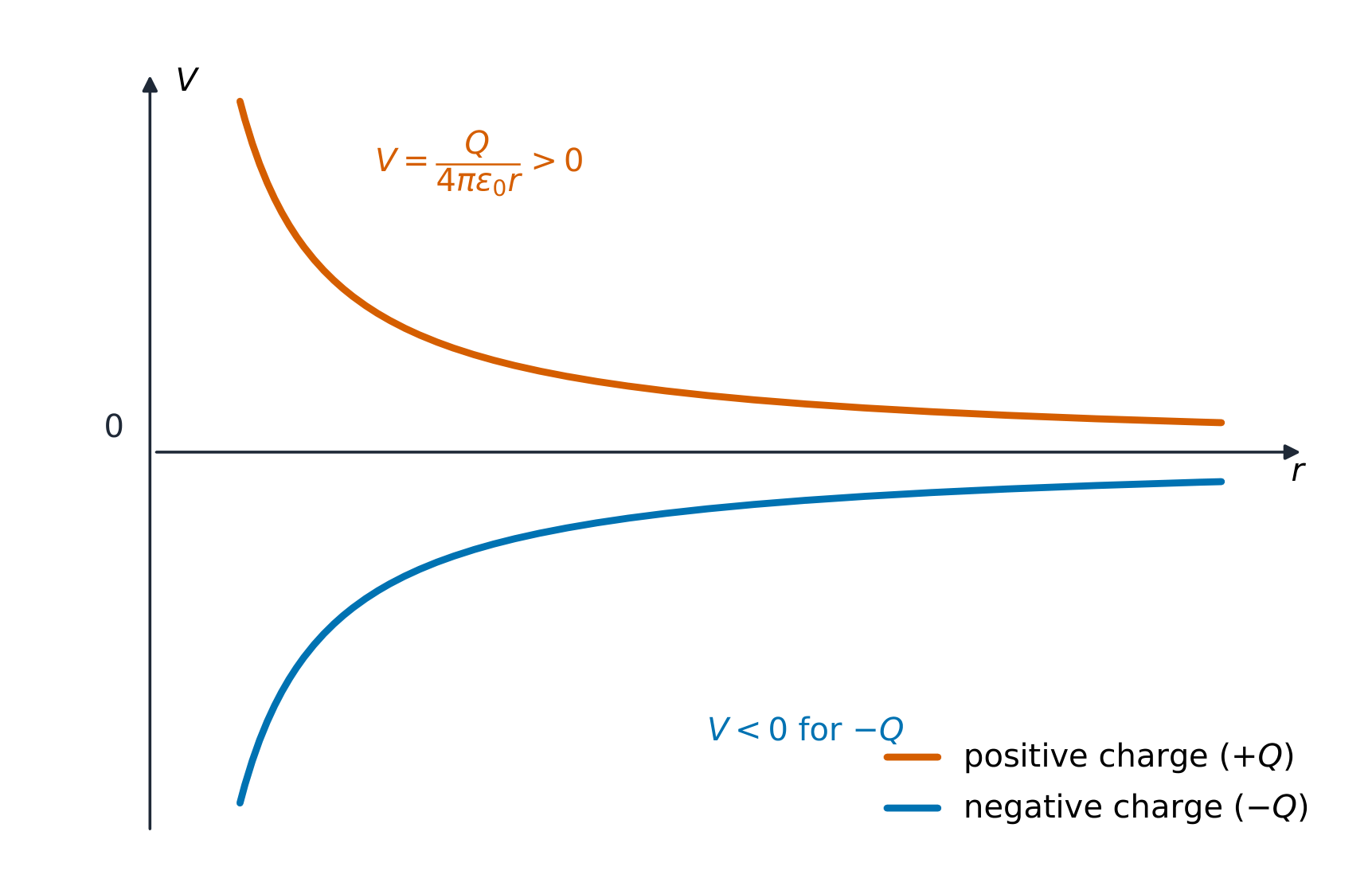
הפוטנציאל סמוך לטען נקודתי משתנה לפי 1/r
מפות שטח פוטנציאל
קו שטח פוטנציאל (נקרא גם איזוליין) מחבר נקודות בעלות אותו פוטנציאל. ארבעה כללים מאפשרים לקרוא כל מפה:
איזולינים הם ניצבים לקווי השדה בכל מקום שבו הם חוצים אותם.
$\vec{E}$ מצביע מ$V$ גבוה ל$V$ נמוך – לעולם לא לאורך קו מתח. הזזת מטען לאורך קו מתח אינה דורשת עבודה.
איזולינים צפופים משמעותם שדה חזק: $E\approx-\Delta V/\Delta x$.
ניתן לשרטט את מפת השדה מתוך מפת איזולינים, ואת מפת האיזולינים מתוך מפת השדה.
קווי שטח פוטנציאל סביב דופול חוצים את קווי השדה בזווית ישרה
כישור מבחן. נתונה מפה עם קווי מתח המרוחקים זה מזה ב-$10\ \text{V}$, הערך הממוצע בין קווים הוא כ-$2\ \text{cm}$. חשב את $E\approx\dfrac{10}{0.02}=500\ \text{V/m}$, שמצביע מהקו בעל הערך הגבוה אל הקו בעל הערך הנמוך. העבודה שבוצעה על ידי גורם חיצוני בהזזת מטען $q$ לאט מ-$A$ ל-$B$ היא $W=q(V_B-V_A)$ – מסלול ההזזה אינו משנה.
קווי מתח גבוה: אנרגיה פוטנציאלית חשמלית מומרת ומועברת כתורעה במתח גבוה
Explore · חקור
Field lines and the potential around a charge · קווי שדה והפוטנציאל סביב מטען
Electric potential is the energy per unit charge. It falls off with distance from a positive charge; the field lines point from high potential to low. · פוטנציאל חשמלי הוא האנרגיה ליחידת מטען. הוא יורד ככל שהמרחק ממטען חיובי גדל; קווי השדה מכוונים מפוטנציאל גבוה לנמוך.
Conservation of Electric Energy · שימור אנרגיה חשמלית
Syllabus · סיילבוס
English
Learning Objective 9.3.A: Describe changes in a system due to a difference in electric potential between two locations.
9.3.A.1 When a charged object moves between two locations with different electric potentials, the resulting change in the electric potential energy of the object-field system is given by the following equation.
Equation:$\Delta U_E = q\Delta V$
9.3.A.2 The movement of a charged object between two points with different electric potentials results in a change in kinetic energy of the object consistent with the conservation of energy.
עברית
מטרות הלמידה 9.3.A: לתאר שינויים במערכת כתוצאה מהפרש בפוטנציאל חשמלי בין שני מיקומים.
9.3.A.1 כאשר גוף טעון נע בין שני מיקומים עם פוטנציאלים חשמליים שונים, השינוי הנובע באנרגיה הפוטנציאלית החשמלית של מערכת הגוף-שדה נתון על ידי המשוואה הבאה.
משוואה:$\Delta U_E = q\Delta V$
9.3.A.2 תנועת גוף טעון בין שתי נקודות עם פוטנציאלים חשמליים שונים גורמת לשינוי באנרגיה הקינטית של הגוף תואם לשימור האנרגיה.
Source: College Board AP Course and Exam Description · מקור: תיאור הקורס והמבחן של College Board AP
English
When a charge $q$ moves between two points that differ in potential by $\Delta V$, the potential energy of the charge–field system changes by
$$\Delta U_E=q\,\Delta V.$$
If only the electric force acts, total energy is conserved, so the kinetic energy changes by the opposite amount:
$$\Delta K=-\Delta U_E=-q\,\Delta V.$$
Watch the two signs together: a positive charge speeds up when it moves to lower potential, while a negative charge speeds up when it moves to higher potential. Both are just the system trading potential energy for kinetic energy. This is how particle accelerators give charged particles their energy, and it underlies energy analysis in circuits.
Worked example. A proton ($q=1.6\times10^{-19}\ \text{C}$, $m=1.67\times10^{-27}\ \text{kg}$) starts at rest and is accelerated through a potential drop of $500\ \text{V}$ (it moves to lower potential, so $\Delta V=-500\ \text{V}$ and $\Delta K=-q\,\Delta V=+8.0\times10^{-17}\ \text{J}$). Setting $\Delta K=\tfrac12 mv^2$:
Exam skill. Choose energy methods, not kinematics, whenever the field is non-uniform or the path curves: only the end-point potentials matter. A typical FRQ chain is $q\,\Delta V \to \Delta K \to v$, with one line of justification: "the electric force is conservative, so energy is conserved."
עברית
כאשר מטען $q$ זז בין שתי נקודות שהפרש הפוטנציאל ביניהן הוא $\Delta V$, האנרגיה הפוטנציאלית של מערכת המטען-שדה משתנה ב-
$$\Delta U_E=q\,\Delta V.$$
אם רק הכוח החשמלי פועל, האנרגיה הכוללת שמורה, ולכן האנרגיה הקינטית משתנה בכמות ההפוכה:
$$\Delta K=-\Delta U_E=-q\,\Delta V.$$
הסתכלו על שני הסימנים יחד: מטען חיובי מאיץ כאשר הוא זז ל-פוטנציאל נמוך, בעוד שמטען שלילי מאיץ כאשר הוא זז ל-פוטנציאל גבוה. שניהם פשוט מחליפים את האנרגיה הפוטנציאלית באנרגיה קינטית. זוהי הדרך שבה מאיצי חלקיקים מספקים לחלקיקים טעונים אנרגיה, והיא מהווה בסיס לניתוח אנרגטי במעגלים.
דוגמה פתורה. פרוטון ($q=1.6\times10^{-19}\ \text{C}$, $m=1.67\times10^{-27}\ \text{kg}$) מתחיל ממצב רגיעה ומאיץ בשטח פוטנציאל של ⟨$500\ \text{V}$⟩ (הוא זז לפוטנציאל נמוך, ולכן $\Delta V=-500\ \text{V}$ ו-$\Delta K=-q\,\Delta V=+8.0\times10^{-17}\ \text{J}$). נקבע $\Delta K=\tfrac12 mv^2$:
כישור למבחן. בחרו בשיטות אנרגטיות ולא בקינמטיקה, כאשר השדה אינו אחיד או שהמסלול מתעקם: רק פוטנציאלי הנקודות הקצה חשובים. שרשרת FRQ אופיינית היא $q\,\Delta V \to \Delta K \to v$, עם שורת נימוק אחת: "הכוח החשמלי הוא שימורי, ולכן האנרגיה שמורה."
9.3
Exam tips · טיפים לבחינות
English
Relate field and potential by $V=-\int \vec E\cdot d\vec l$ and $\vec E=-\nabla V$ (in 1-D, $E_x=-\tfrac{dV}{dx}$).
Potential is a scalar — add contributions with signs, no vector components needed.
Potential energy of a pair is $U=\tfrac{1}{4\pi\varepsilon_0}\tfrac{q_1 q_2}{r}$; use energy conservation for a charge's speed.
Know that no work is done moving along an equipotential, which is perpendicular to $\vec E$.
Choose the zero of potential (usually infinity) and state it.
עברית
קשר בין שדה לפוטנציאל באמצעות $V=-\int \vec E\cdot d\vec l$ ו$\vec E=-\nabla V$ (ב-1-D, $E_x=-\tfrac{dV}{dx}$).
פוטנציאל הוא סקלרי – יש להוסיף תרומות עם סימנים, ללא צורך ברכיבי וקטור.
האנרגיה הפוטנציאלית של זוג היא $U=\tfrac{1}{4\pi\varepsilon_0}\tfrac{q_1 q_2}{r}$; השתמשו בשימור אנרגיה כדי למצוא את מהירותו של מטען.
לדעת שאין עבודה נעשית בהזזה לאורך שטח פוטנציאל, שהוא ניצב ל-$\vec E$.
בחר את אפס הפוטנציאל (בדרך כלל אינסוף) וצין אותו.
Interactive lessons on this topic · שיעורים אינטראקטיביים בנושא זה
Work through it step by step, with instant-check exercises. · לעבור על הדברים צעד אחר צעד, עם תרגילים לבדיקה מיידית.
More topics in AP Physics C: Electricity and Magnetism · פיזיקה AP C: חשמל ומגנטיות · נושאים נוספים בAP Physics C: Electricity and Magnetism · פיזיקה AP C: חשמל ומגנטיות
Pick one and the site follows you — notes, papers, videos and practice all open on it. · בחרו נושא אחד והאתר יעקוב אחריו — הערות, מסמכים, וידאו ותרגולים פתוחים בו.
Type to search notes, lessons, code, vocabulary and past-paper questions across every subject. · הקלד כדי לחפש הערות, שיעורים, קוד, אוצר מילים ושאלות מבחנים בכל הנושאים.