| Learning Objective | Essential Knowledge |
|---|---|
8.1.A |
|
8.1.B |
|
8.1.C |
Boundary statement: AP Physics C: Electricity & Magnetism only expects students to make calculations of the electric force between four or fewer interacting charged objects or systems. The analysis of the resulting electric force from more charges is allowed in situations of high symmetry. Note that students are expected to calculate the electric fields of charge distributions, as described in Topics 8.4 and 8.6. |
Tips · טיפים
AP Physics C: חשמל ומגנטיות היא הקורס בחשמל ומגנטיות המבוסס על גזירה: מטענים, שדות ו-חוק גאוס; פוטנציאל חשמלי; מוליכים ו-קבלים; מעגלים; שדות מגנטיים; והשראת אלקטרומגנטית. לרוב נלמד לאחר מכניקה והוא מצפה רמת גזירה זו.
חוק גאוס וחוק אמפיר מחליטים איך הקורס הזה מרגיש. שניהם בעצם מדברים על בחירת משטח או לולאה שהופכת את האינטגרל לפשוט — כשרון שאתם בונים על ידי ביצוע של הרבה, ולא על ידי קריאת החוק. סימטריה היא כל המשחק.
שאלות השראה עונשות טעויות סימן יותר מכל דבר אחר, ולכן קבעו שיטת סימן אחת לכיוון הפlux והשתמשו בה בכל פעם.
ההערות מכסות את חוק גאוס ועד למשוואות מקסוול, יחידה אחר יחידה, עם הגזירה הווקטוריאלית מפורטת. הספרייה מכילה את ה-FRQs שפורסמו; הנקודות הקשות ביותר ב-E&M הן בחירת הסימטריה הנכונה לפני האינטגרציה, ולכן הדוגמאות מתחילות משם.
-
8
Electric Charges, Fields, and Gauss's Law · מטענים חשמליים, שדות חשמלי וחוק גאוס
Watch lesson · צפה בשיעור8.1
Electric Charge and Electric Force
Syllabus · סיילבוס
Source: College Board AP Course and Exam Description · מקור: תיאור הקורס והמבחן של College Board AP
Electric charge 电荷 comes in positive and negative; like charges repel, opposites attract. Charge is quantized 量子化 – every charge is a whole-number multiple of the elementary charge 基本电荷 $e=1.6\times10^{-19}\ \text{C}$ – and obeys conservation of charge 电荷守恒: charge is never created or destroyed, only moved. The force between two point charges 点电荷 is Coulomb's law 库仑定律:
$$\vec{F}=\frac{1}{4\pi\varepsilon_0}\frac{q_1 q_2}{r^2}\,\hat{r},$$an inverse-square 平方反比 force along the line joining them, with $\dfrac{1}{4\pi\varepsilon_0}=k=9.0\times10^{9}\ \text{N}\cdot\text{m}^2/\text{C}^2$. For several charges (AP uses four or fewer, unless symmetry helps), add the force vectors on the charge you care about – superposition 叠加.
Charge is a fundamental property 基本属性 of matter, and a point charge is a model that ignores the size of a charged object. The constant $\varepsilon_0$ is the permittivity of free space 真空介电常数 – a material property of the vacuum. The permittivity of matter differs from $\varepsilon_0$, set by how easily the material polarizes, which is why a dielectric between charges weakens the force. Note too that although the electric force is far stronger than gravity, gravity dominates at astronomical scales because large bodies are nearly neutral.
Worked example. Two $+2.0\ \mu\text{C}$ charges sit $0.30\ \text{m}$ apart: $F=\dfrac{kq_1q_2}{r^2}=\dfrac{9.0\times10^{9}(2.0\times10^{-6})^2}{(0.30)^2}=0.40\ \text{N}$, repulsive.
Worked example (vectors). Charges $+3.0\ \mu\text{C}$ and $-3.0\ \mu\text{C}$ sit at two corners of a right angle, each $0.30\ \text{m}$ from a $+1.0\ \mu\text{C}$ charge at the corner. Each exerts $F=\dfrac{(9.0\times10^{9})(3.0\times10^{-6})(1.0\times10^{-6})}{0.09}=0.30\ \text{N}$ – one a push, one a pull, at right angles to each other. The net force is $F_{\text{net}}=\sqrt{0.30^2+0.30^2}=0.42\ \text{N}$, pointing between them. Never add magnitudes blindly: components first.
Explore · חקורExplore the field of a source charge · חקרו שדה של מטען מקור
Change the charge's sign and size. Lines point away from positive and toward negative, and their $1/r^2$ crowding near the charge mirrors why Coulomb's force $F = k\,|q_1 q_2|/r^2$ weakens with distance. · שנו את ה-סימן והגודל של המטען. הקווים מצביעים למרחק ממטען חיובי ולכיוון מטען שלילי, והעיסוק שלהם ב-$1/r^2$ ליד המטען מדמה מדוע כוח קולון $F = k\,|q_1 q_2|/r^2$ חולש עם המרחק.
Vocabulary · מילון מונחים Train · אימוןEnglish עברית Electric charge/ɪˈlektrɪk tʃɑːdʒ/ מטען חשמלי quantized/ˈkwɒntaɪzd/ כמותי elementary charge/ˌelɪˈmentəri tʃɑːdʒ/ מטען יסודי conservation of charge/ˌkɒnsəˈveɪʃn ɒv tʃɑːdʒ/ שימור מטען point charges/pɔɪnt ˈtʃɑːdʒɪz/ טענות נקודתיות Coulomb's law/ˈkuːlɒmz lɔː/ חוק קולון inverse-square/ɪnˈvɜːs skweə/ הפוך-ריבועי superposition/ˌsuːpəpəˈzɪʃn/ הפרעה (סופרפוזיציה) fundamental property/ˌfʌndəˈmentl ˈprɒpəti/ תכונה יסודית permittivity of free space/ˌpɜːmɪˈtɪvəti ɒv friː speɪs/ הפרמיטיביות של ריק 8.2
Electric Charge and the Process of Charging
Syllabus · סיילבוס
EnglishLearning Objective 8.2.A: Describe the behavior of a system using conservation of charge.
- 8.2.A.1 The net charge or charge distribution of a system can change in response to the presence of, or changes in, the net charge or charge distribution of other systems.
- 8.2.A.1.i The net charge of a system can change due to friction or contact between systems.
- 8.2.A.1.ii Induced charge separation occurs when the electrostatic force between two systems alters the distribution of charges within the systems, resulting in the polarization of one or both systems.
- 8.2.A.1.iii Induced charge separation can occur in neutral systems.
- 8.2.A.2 Any change to a system's net charge is due to a transfer of charge between the system and its surroundings.
- 8.2.A.2.i The charging of a system typically involves the transfer of electrons to and from the system.
- 8.2.A.2.ii The net charge of a system will be constant unless there is a transfer of charge to or from the system.
- 8.2.A.3 Grounding involves electrically connecting a charged object to a much larger and approximately neutral system (e.g., Earth).
עבריתמטרות למידה 8.2.A: לתאר את התנהגות מערכת באמצעות שימור המטען.
- 8.2.A.1 המטען הכולל או חלוקת המטען של מערכת יכולים להשתנות כתוצאה מהנוכחות, או משנויים, במטען הכולל או בחלוקת המטען של מערכות אחרות.
- 8.2.A.1.i המטען הכולל של מערכת יכול להשתנות בשל חיכוך או מגע בין מערכות.
- 8.2.A.1.ii הפרדת מטען מושרית מתרחשת כאשר הכוח האלקטרוסטטי בין שתי מערכות משנה את חלוקת המטענים בתוך המערכות, ומוביל לקיטוב אחת או שתי המערכות.
- 8.2.A.1.iii הפרדת מטען מושרית יכולה להתרחש במערכות ניטרליות.
- 8.2.A.2 כל שינוי במטען הכולל של מערכת נובע ממעבר מטען בין המערכת לסביבתה.
- 8.2.A.2.i טעינת מערכת כוללת בדרך כלל מעבר אלקטרונים אל תוך המערכת ומהמערכת.
- 8.2.A.2.ii המטען הכולל של מערכת יישאר קבוע אלא אם כן ישנן מעברי מטען אל תוכה או ממנה.
- 8.2.A.3 חיבור לאדמה (Grounding) כולל חיבור חשמלי של גוף טעון למערכת גדולה בהרבה ובסביבות הניטרלית (למשל, כדור הארץ).
Source: College Board AP Course and Exam Description · מקור: תיאור הקורס והמבחן של College Board AP
A conductor 导体 lets charge move freely; an insulator 绝缘体 holds it in place. Objects gain net charge three ways:
- Charging by friction 摩擦起电: rubbing transfers electrons from one surface to the other.
- Charging by conduction 传导起电: touching a charged object shares charge of the same sign.
- Charging by induction 感应起电: a nearby charge pushes the conductor's charge apart; ground 接地 the far side, remove the ground wire first, and the conductor is left with the opposite sign – all without contact.
An insulator cannot pass charge, but it can develop polarization 极化: its molecules stretch or turn so one face is slightly positive and the other slightly negative. That is why a charged comb picks up neutral paper scraps. An electroscope 验电器 shows net charge by its leaves repelling; on any isolated conductor the excess charge sits entirely on the outer surface.
Explore · חקורExplore charging by rubbing · חקרו טעינה בשחיקה
Rubbing transfers electrons onto the object, leaving it negative. A charged object then attracts a neutral wall or hair (by polarization) but repels another like-charged object — the same electron transfer behind friction, conduction, and induction. · שחיקה מעבירה אלקטרונים למצופה, משאירה אותו טעון שלילית. אובייקט טעון אז מושך קיר ניטרלי או שיער (באמצעות קיטוב) אך דוחה אובייקט אחר עם מטען דומה — אותה העברת אלקטרונים עומדת מאחורי חיכוך, הולכה ואינדוקציה.
Vocabulary · מילון מונחים Train · אימוןEnglish עברית conductor/kənˈdʌktə/ מו Interructor insulator/ˈɪnsjuːleɪtə/ בודד חשמלי Charging by friction/ˈtʃɑːdʒɪŋ baɪ ˈfrɪkʃn/ טעינה בשחיקה Charging by conduction/ˈtʃɑːdʒɪŋ baɪ kənˈdʌkʃn/ טעינה בהולכה Charging by induction/ˈtʃɑːdʒɪŋ baɪ ɪnˈdʌkʃn/ טעינה באינדוקציה ground/ɡraʊnd/ הארקה polarization/ˌpəʊləraɪˈzeɪʃn/ קיטוב electroscope/ɪˌlektrəʊˈskəʊp/ אלקטרוסקופ 8.3
Electric Fields
Syllabus · סיילבוס
Learning Objective Essential Knowledge 8.3.A
Describe the electric field produced by a charged object or configuration of point charges.- 8.3.A.1 Electric fields may originate from charged objects.
- 8.3.A.2 The electric field at a given point is the ratio of the electric force exerted on a test charge at the point to the charge of the test charge.
- Relevant equation: $\vec{E} = \dfrac{\vec{F}_E}{q}$
- 8.3.A.2.i A test charge is a point charge of small enough magnitude such that its presence does not significantly affect an electric field in its vicinity.
- 8.3.A.2.ii An electric field points away from isolated positive charges and toward isolated negative charges.
- 8.3.A.2.iii The electric force exerted on a positive test charge by an electric field is in the same direction as the electric field.
- 8.3.A.3 The electric field is a vector quantity and can be represented in space using vector field maps.
- 8.3.A.3.i The net electric field at a given location is the vector sum of individual electric fields created by nearby charged objects.
- 8.3.A.3.ii Electric field maps use vectors to depict the magnitude and direction of the electric field at many locations within a given region.
- 8.3.A.3.iii Electric field line diagrams are simplified models of electric field maps and can be used to determine the relative magnitude and direction of the electric field at any position in the diagram.
8.3.B
Describe the electric field generated by charged conductors or insulators.- 8.3.B.1 While in electrostatic equilibrium, the excess charge of a conductor is distributed on the surface of the conductor, and the electric field within the conductor is zero.
- 8.3.B.1.i At the surface of a charged conductor, the electric field is perpendicular to the surface.
- 8.3.B.1.ii The electric field outside an isolated sphere with spherically symmetric charge distribution is the same as the electric field due to a point charge with the same net charge as the sphere located at the center of the sphere.
- 8.3.B.2 While in electrostatic equilibrium, the excess charge of an insulator is distributed throughout the interior of the insulator as well as at the surface, and the electric field within the insulator may have a nonzero value.
Source: College Board AP Course and Exam Description · מקור: תיאור הקורס והמבחן של College Board AP
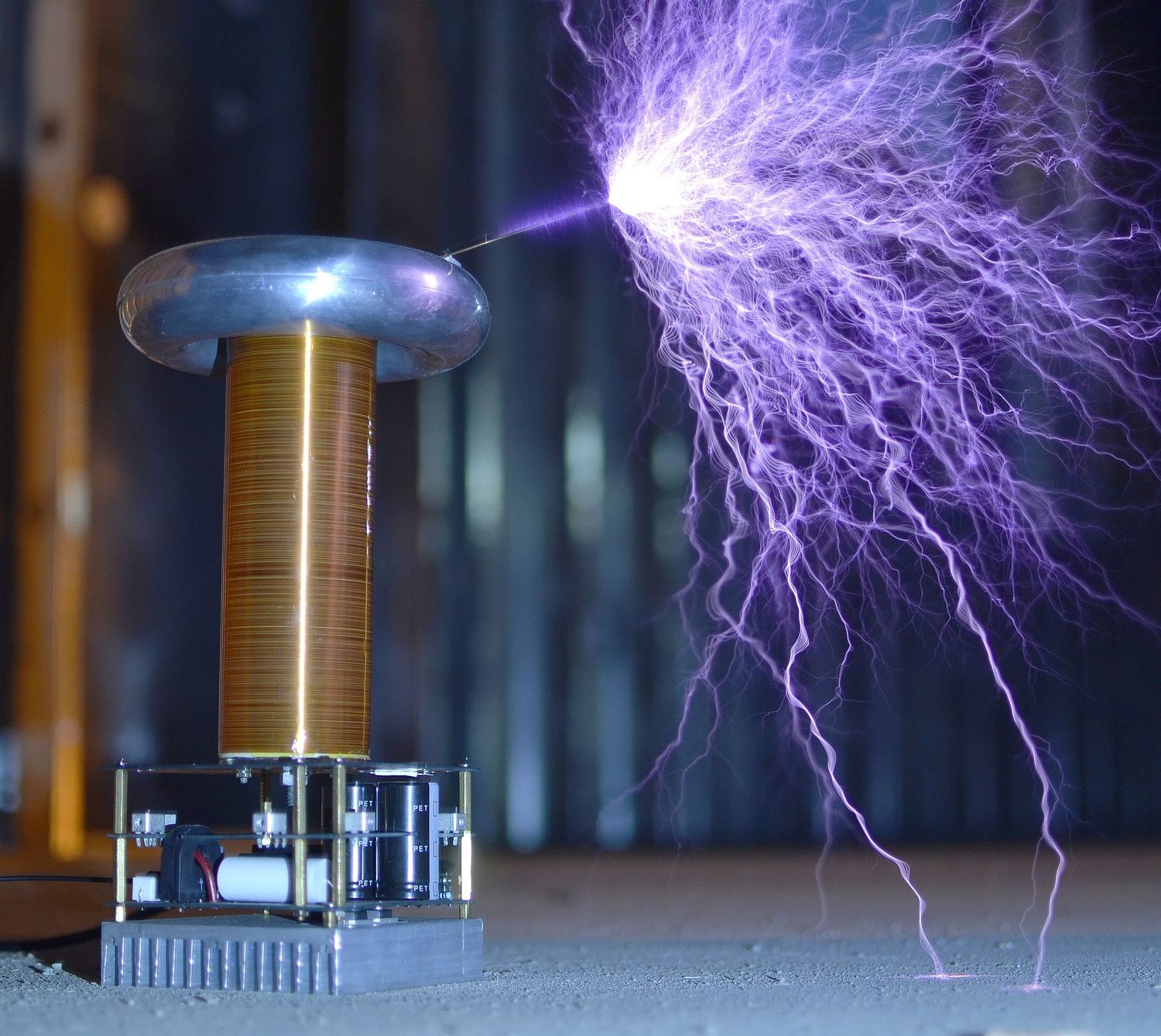
The electric field of a dipole A Tesla coil throws sparks: it raises the voltage so high that the electric field ionizes the surrounding air, and charge leaps across as a visible discharge The electric field 电场 at a point is the force per unit charge that a small positive test charge 检验电荷 would feel there:
$$\vec{E}=\frac{\vec{F}}{q},\qquad \vec{E}=\frac{1}{4\pi\varepsilon_0}\frac{q}{r^2}\,\hat{r}\ \text{(point charge)}.$$A charge placed in a field feels $\vec{F}=q\vec{E}$ – positive charges along the field, negative charges against it. Fields from several sources add as vectors (superposition again). Field lines 电场线 make the field visible: they point away from positive charge and toward negative, their density shows the strength, and they never cross.
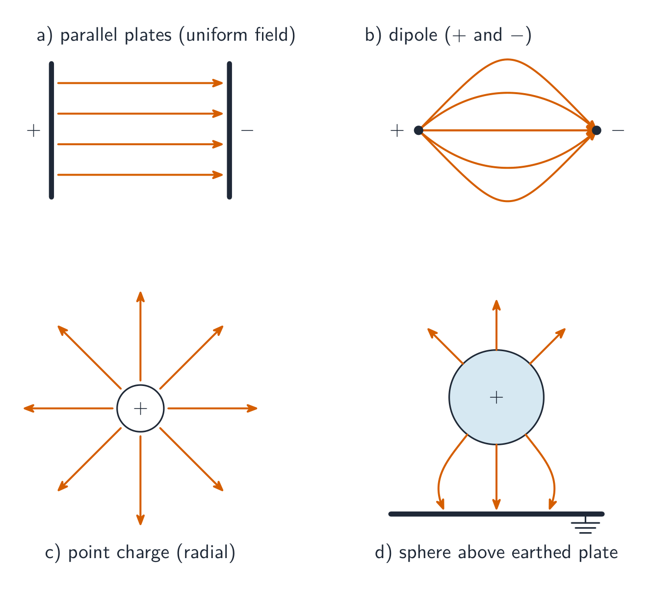
Electric field-line patterns for parallel plates, a dipole, and a point charge 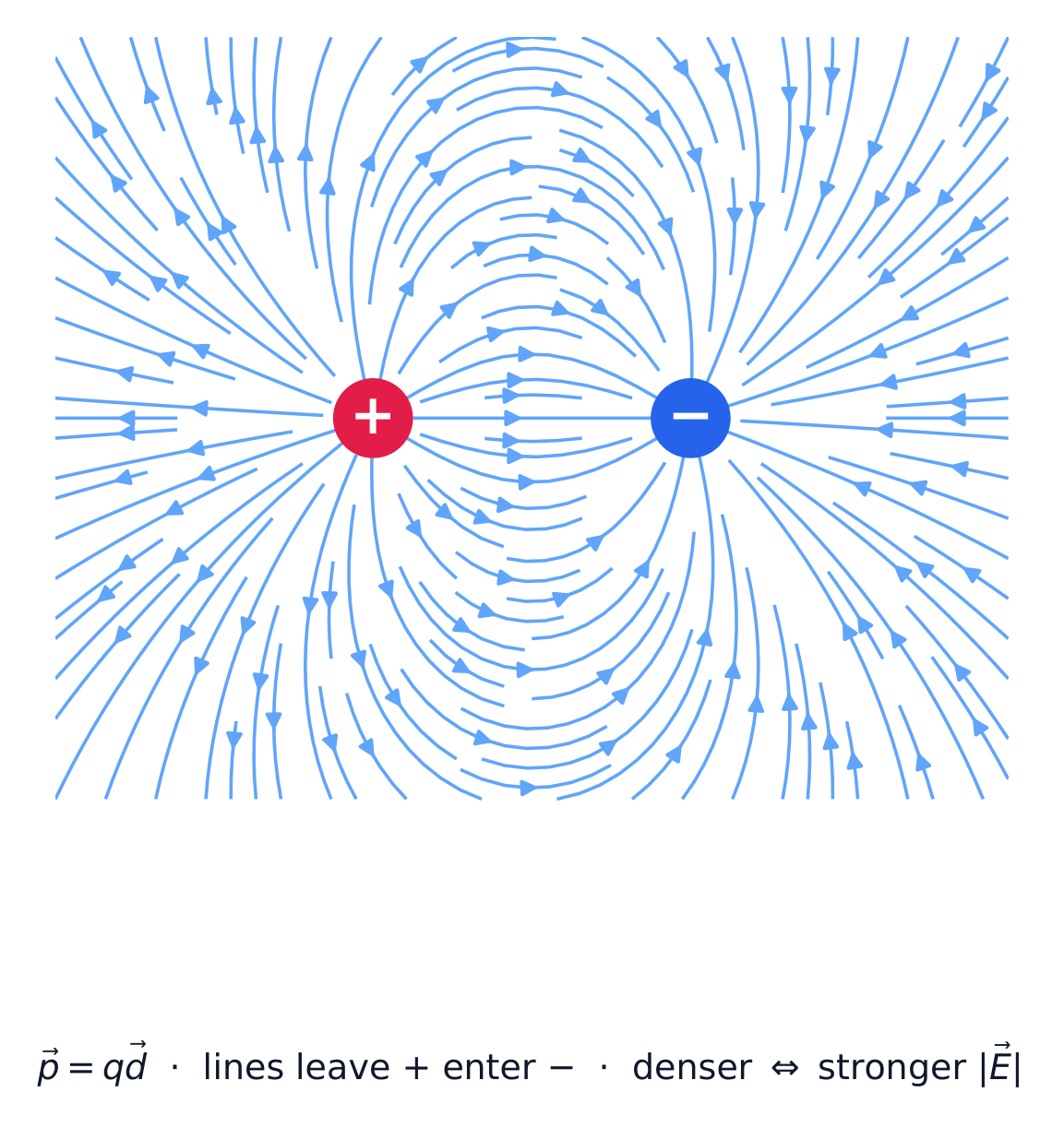
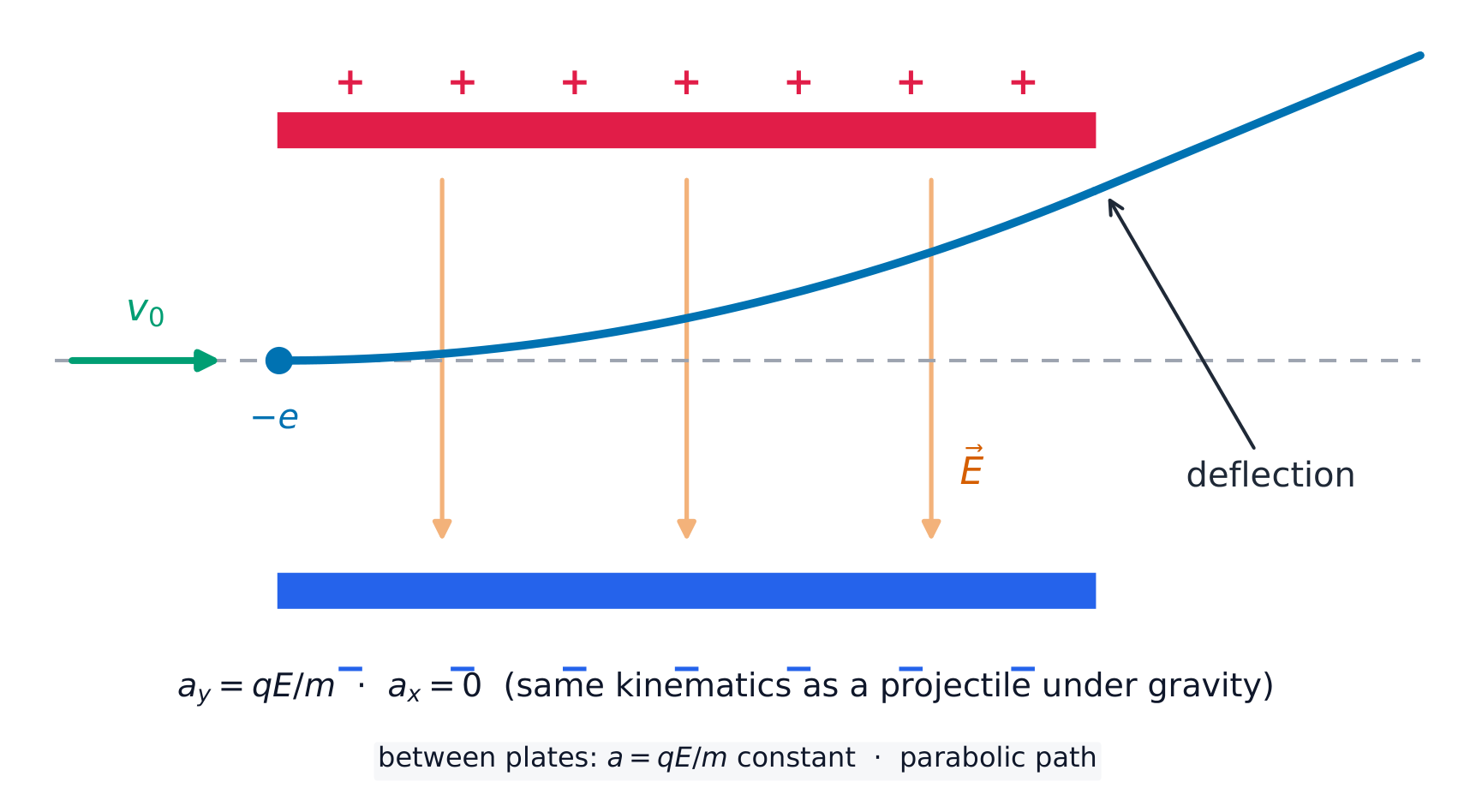
Electric field lines of a dipole point from the positive to the negative charge In a uniform 均匀 field a charge feels a constant force, so it accelerates uniformly – launched sideways, it follows a parabola, just like a projectile in gravity.
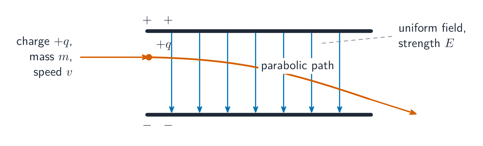
A charge crossing a uniform field follows a parabolic path 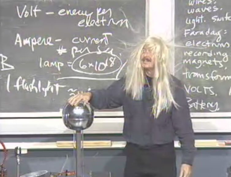
Charge spreads over the dome and onto the hair; like charges repel, so the strands push apart Explore · חקורExplore field lines of a point charge · חקרו קווי שדה של מטען נקודתי
Set the charge positive or negative. Field lines start on positive and end on negative charge, never cross, and crowd together where $\vec{E}$ is strongest — the line density is proportional to the field magnitude. · הגדירו את המטען כחיובי או שלילי. קווי השדה מתחילים על מטען חיובי ומסתיימים על מטען שלילי, לעולם אינם נחתכים, ומצטופפים שם שבהם $\vec{E}$ הוא החזק ביותר — הצפיפות בקווים פרופורציונלית לגודל השדה.
Vocabulary · מילון מונחים Train · אימוןEnglish עברית electric field/ɪˈlektrɪk fiːld/ שדה חשמלי test charge/test tʃɑːdʒ/ מטען בדיקה Field lines/fiːld laɪnz/ קווי שדה uniform/ˈjuːnɪfɔːm/ אחיד 8.4
Electric Fields of Charge Distributions
Syllabus · סיילבוס
Learning Objective Essential Knowledge 8.4.A
Describe the electric field resulting from a given charge distribution.- 8.4.A.1 Expressions for the electric field of specified charge distributions can be found using integration and the principle of superposition.
- Relevant equation: $\vec{E} = \dfrac{1}{4\pi\varepsilon_0} \displaystyle\int \dfrac{dq}{r^2} \hat{r}$
- 8.4.A.2 Symmetry considerations of certain charge distributions can simplify analysis of the electric field resulting from those charge distributions.
Boundary statement: AP Physics C: Electricity & Magnetism only expects students to use calculus to find the electric field resulting from the following charge distributions and locations: an infinitely long, uniformly charged wire or cylinder at a distance from its central axis, a thin ring of charge at a location along the axis of the ring, a semicircular arc or part of a semicircular arc at its center, and a finite wire or line charge at a point collinear with the line charge or at a location along its perpendicular bisector.
Source: College Board AP Course and Exam Description · מקור: תיאור הקורס והמבחן של College Board AP
For a continuous charge distribution 连续电荷分布, cut the object into pieces $dq$ and integrate their point-charge fields:
$$\vec{E}=\frac{1}{4\pi\varepsilon_0}\int \frac{dq}{r^2}\,\hat{r}.$$Write $dq$ using the right density: $\lambda\,dl$ with the linear charge density 线电荷密度 (a line or ring), $\sigma\,dA$ with the surface charge density 面电荷密度, or $\rho\,dV$ with the volume charge density 体电荷密度. Then use symmetry 对称性 to cancel components before integrating – that sentence is usually a scored step. AP's calculus cases: a finite line (collinear point or perpendicular bisector), an infinite wire or cylinder, a ring on its axis, and an arc at its centre.
Worked example (ring, on axis). A ring of radius $R$ carries charge $Q$. At a point $z$ along the axis, each element is a distance $\sqrt{R^2+z^2}$ away, and by symmetry the sideways components cancel, leaving only the axial part ($\cos\alpha=z/\sqrt{R^2+z^2}$):
$$E_z=\frac{1}{4\pi\varepsilon_0}\int\frac{dq}{R^2+z^2}\cdot\frac{z}{\sqrt{R^2+z^2}}=\frac{1}{4\pi\varepsilon_0}\frac{Qz}{(R^2+z^2)^{3/2}}.$$Check the limits: $E=0$ at the centre ($z=0$), and far away ($z\gg R$) it becomes $kQ/z^2$ – a point charge, as it must.
Vocabulary · מילון מונחים Train · אימוןEnglish עברית continuous charge distribution/kənˈtɪnjuːəs tʃɑːdʒ ˌdɪstrɪˈbjuːʃn/ חלוקת טענה רציפה linear charge density/ˈlɪnɪə tʃɑːdʒ ˈdensɪti/ צפיפות טענה ליניארית surface charge density/ˈsɜːfɪs tʃɑːdʒ ˈdensɪti/ צפיפות מטען פני שטח volume charge density/ˈvɒljuːm tʃɑːdʒ ˈdensɪti/ צפיפות טענה נפחית symmetry/ˈsɪmətri/ סימטריה 8.5
Electric Flux
Syllabus · סיילבוס
Learning Objective Essential Knowledge 8.5.A
Describe the electric flux through an arbitrary area or geometric shape.- 8.5.A.1 Flux describes the amount of a given quantity that passes through a given area.
- 8.5.A.2 For an electric field $\vec{E}$ that is constant across an area $\vec{A}$, the electric flux through the area is defined as $\Phi_E = \vec{E} \bullet \vec{A}$.
- 8.5.A.2.i The direction of the area vector is defined as perpendicular to the plane of the surface and outward from a closed surface.
- 8.5.A.2.ii The sign of flux is given by the dot product of the electric field vector and the area vector.
- 8.5.A.3 The total electric flux passing through a surface is defined by the surface integral of the electric field over the surface.
- Relevant equation: $\Phi_E = \displaystyle\int \vec{E} \cdot d\vec{A}$
Source: College Board AP Course and Exam Description · מקור: תיאור הקורס והמבחן של College Board AP
Electric flux & Gauss's law Electric flux 电通量 measures how much field passes through a surface:
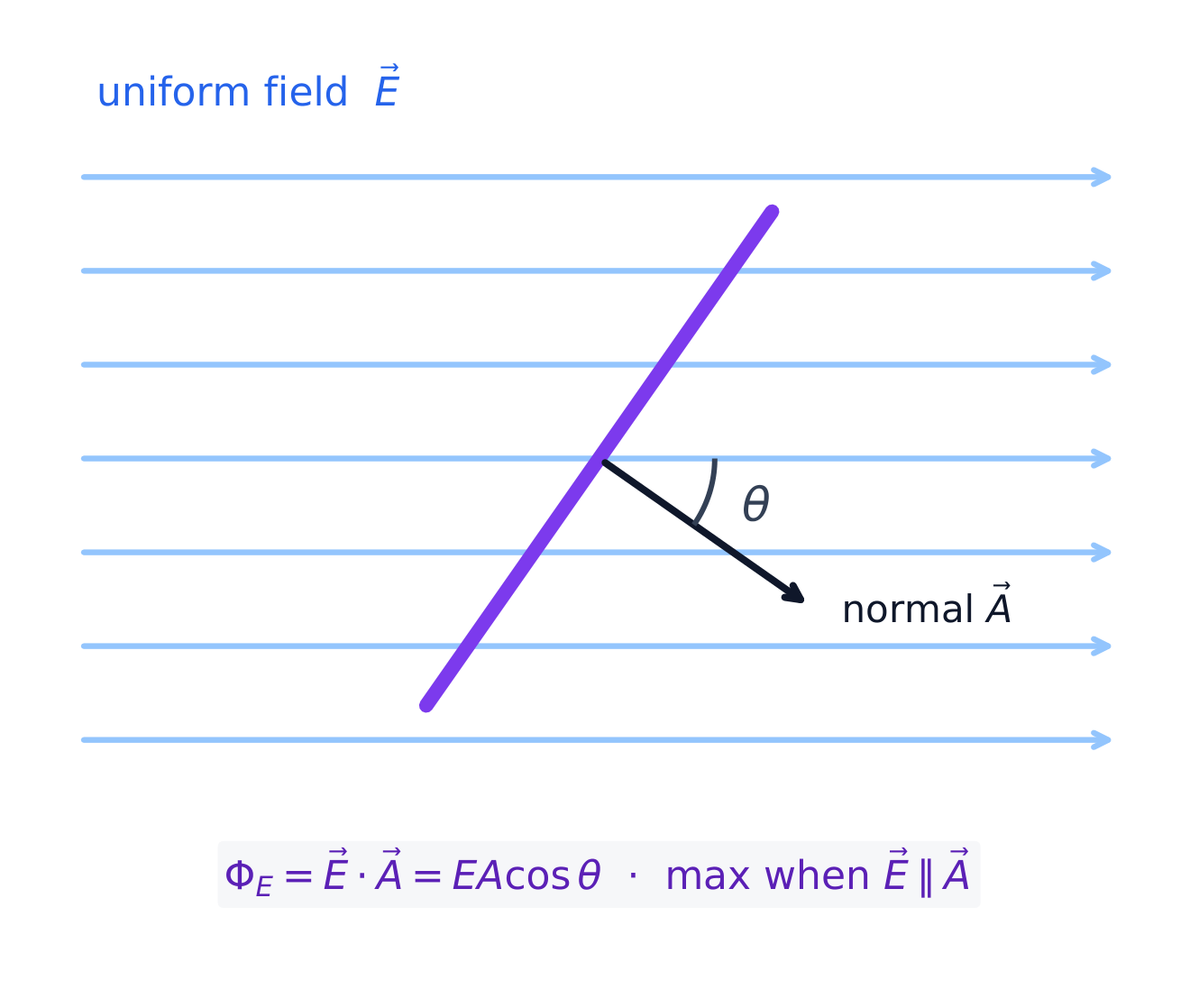
$$\Phi_E=\int \vec{E}\cdot d\vec{A}.$$For a uniform field through a flat area, $\Phi_E=EA\cos\theta$, where the area vector 面积矢量 is perpendicular to the surface. Flux is positive where field lines exit a closed surface and negative where they enter – only the perpendicular component of $\vec{E}$ counts.
Electric flux through a surface depends on the angle between the field and the surface normal Vocabulary · מילון מונחים Train · אימוןEnglish עברית Electric flux/ɪˈlektrɪk flʌks/ זרם חשמלי area vector/ˈeərɪə ˈvektə/ ווקטור שטח 8.6
Gauss's Law
Syllabus · סיילבוס
Learning Objective Essential Knowledge 8.6.A
Describe the properties of a charge distribution by applying Gauss's law.- 8.6.A.1 Gauss's law relates electric flux through a Gaussian surface to the charge enclosed by that surface.
- Relevant equations: $\Phi_E = \dfrac{q_{\text{enc}}}{\varepsilon_0}$ and $\displaystyle\oint \vec{E} \cdot d\vec{A} = \dfrac{q_{\text{enc}}}{\varepsilon_0}$
- 8.6.A.2 A Gaussian surface is a three-dimensional, closed surface.
- 8.6.A.3 The total electric flux through a Gaussian surface is independent of the size of the Gaussian surface if the amount of enclosed charge remains constant.
- 8.6.A.4 Gaussian surfaces are typically constructed such that the electric field generated by the enclosed charge is either perpendicular or parallel to different regions of the Gaussian surface, resulting in a simplified surface integral.
- 8.6.A.5 If a function of charge density is given for a charge distribution, the total charge can be determined by integrating the charge density over the length (one dimension), area (two dimensions), or volume (three dimensions) of the charge distribution. For example: $Q_{\text{total}} = \displaystyle\int \rho(\vec{r})\, dV$
- 8.6.A.6 Maxwell's equations are the collection of equations that fully describe electromagnetism. Gauss's law is Maxwell's first equation.
- Relevant equation: $\displaystyle\oint \vec{E} \cdot d\vec{A} = \dfrac{q_{\text{enc}}}{\varepsilon_0}$
Boundary statement: AP Physics C: Electricity & Magnetism only expects students to quantitatively apply Gauss's law to point charges and charge distributions that have spherical, cylindrical, or planar symmetry.
Source: College Board AP Course and Exam Description · מקור: תיאור הקורס והמבחן של College Board AP
Gauss's law 高斯定律 – the first of Maxwell's equations – relates the flux through any closed surface to the charge inside it:
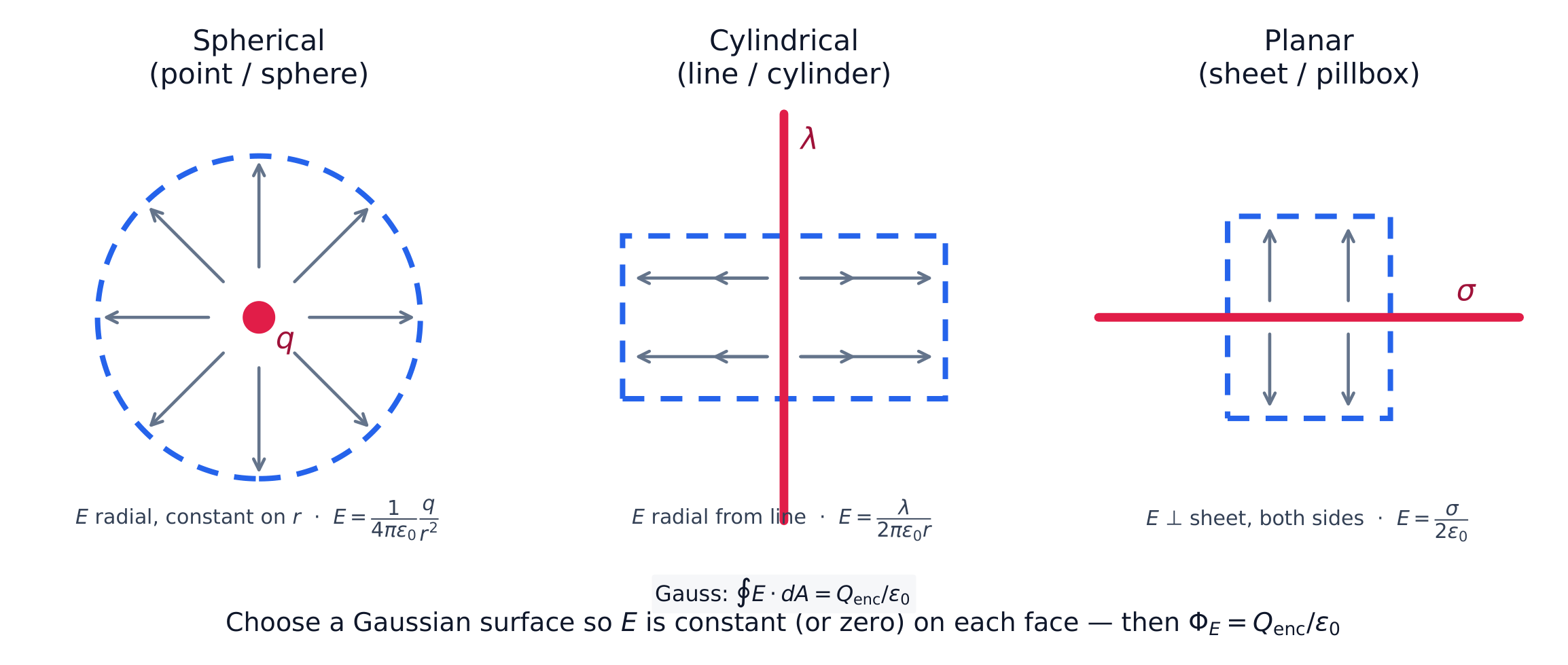
$$\oint \vec{E}\cdot d\vec{A}=\frac{Q_{\text{enc}}}{\varepsilon_0}.$$It is true for any closed surface, but it solves for $E$ only when symmetry lets you choose a Gaussian surface 高斯面 on which $E$ is constant and perpendicular (or parallel, contributing zero). The three symmetries AP tests: spherical symmetry 球对称 (concentric sphere), cylindrical symmetry 柱对称 (coaxial cylinder), and planar symmetry 平面对称 (a straddling "pillbox").
A Gaussian surface is chosen to match the symmetry of the charge Worked example (sphere). Outside a sphere of total charge $Q$, a spherical Gaussian surface of radius $r$ gives $E(4\pi r^2)=Q/\varepsilon_0$, so $E=\dfrac{kQ}{r^2}$ – identical to a point charge at the centre. Inside a uniformly charged solid sphere of radius $R$, the surface encloses only $Q_{\text{enc}}=Q\,r^3/R^3$, so $E=\dfrac{kQr}{R^3}$: zero at the centre, growing linearly to the surface.
Worked example (wire). For an infinite wire with charge per length $\lambda$, take a coaxial cylinder of radius $r$ and length $L$. The ends contribute nothing ($\vec{E}\perp d\vec{A}$), so $E(2\pi rL)=\dfrac{\lambda L}{\varepsilon_0}$ and $E=\dfrac{\lambda}{2\pi\varepsilon_0 r}$. The same pillbox method gives an infinite sheet's field, $E=\dfrac{\sigma}{2\varepsilon_0}$, uniform on both sides.
Exam skill. A full-credit Gauss's-law answer has four parts: name the surface, state the symmetry argument (why $E$ is constant and perpendicular on it), count $Q_{\text{enc}}$, then solve. Skipping the symmetry sentence loses the reasoning point – and remember Gauss's law also explains why $E=0$ inside any conductor in equilibrium.
Vocabulary · מילון מונחים Train · אימוןEnglish עברית Gauss's law/ˈɡaʊsɪz lɔː/ חוק גאוס Gaussian surface/ˈɡaʊʃn ˈsɜːfɪs/ פני גאוס spherical symmetry/sˈferɪkl ˈsɪmətri/ סימטריה כדורית cylindrical symmetry/sɪˈlɪndrɪkl ˈsɪmətri/ סימטריה צילינדרית planar symmetry/ˈpleɪnə ˈsɪmətri/ סימטריה מישורית 8.6
Exam tips
- Use Coulomb's law $F=\tfrac{1}{4\pi\varepsilon_0}\tfrac{q_1 q_2}{r^2}$ and superpose forces as vectors (components, not magnitudes).
- For a continuous charge, integrate $d\vec E$ over $dq=\lambda\,dl,\ \sigma\,dA,\ \rho\,dV$; use symmetry to cancel components.
- The field points away from positive and toward negative charge; draw field lines correctly.
- Distinguish the force on a charge ($\vec F=q\vec E$) from the field the charge creates.
- Keep the constant $k=\tfrac{1}{4\pi\varepsilon_0}$ straight and check units.
- 8.2.A.1 The net charge or charge distribution of a system can change in response to the presence of, or changes in, the net charge or charge distribution of other systems.
-
9
Electric Potential · פוטנציאל חשמלי
Watch lesson · צפה בשיעור9.1
Electric Potential Energy · אנרגיה פוטנציאלית חשמלית
Syllabus · סיילבוס
EnglishLearning Objective 9.1.A: Describe the electric potential energy of a system.
- 9.1.A.1 The electric potential energy of a system of two point charges equals the amount of work required for an external force to bring the point charges to their current positions from infinitely far away.
- 9.1.A.2 The general form for the electric potential energy between two charged objects is given by the equation
- Equation: $U_E = \dfrac{1}{4\pi\varepsilon_0}\dfrac{q_1 q_2}{r} = k\dfrac{q_1 q_2}{r}$.
- 9.1.A.3 The total electric potential energy of a system can be determined by finding the sum of the electric potential energies of the individual interactions between each pair of charged objects in the system.
עבריתמטרת הלמידה 9.1.A: לתאר את האנרגיה הפוטנציאלית חשמלית של מערכת.
- 9.1.A.1 האנרגיה הפוטנציאלית חשמלית של מערכת של שני מטעני נקודה שווה לכמות העבודה הנדרשת מכוח חיצוני להביא את מטעני הנקודה למיקומם הנוכחי מרחק אינסופי.
- 9.1.A.2 הצורה הכללית עבור האנרגיה הפוטנציאלית חשמלית בין שני גופים טעונים נתונה על ידי המשוואה
- משוואה: $U_E = \dfrac{1}{4\pi\varepsilon_0}\dfrac{q_1 q_2}{r} = k\dfrac{q_1 q_2}{r}$.
- 9.1.A.3 את האנרגיה הפוטנציאלית החשמלית הכוללת של מערכת ניתן לקבוע על ידי מציאת הסכום של האנרגיות הפוטנציאליות החשמליות של האינטראקציות הבודדות בין כל זוג של גופים טעונים במערכת.
Source: College Board AP Course and Exam Description · מקור: תיאור הקורס והמבחן של College Board AP
EnglishWhen you push two like charges together, you do work 功 against the electric force. That work is stored by the pair as electric potential energy 电势能:
$$U_E=\frac{1}{4\pi\varepsilon_0}\frac{q_1 q_2}{r}=k\frac{q_1 q_2}{r}.$$$U_E$ is defined as the work an external force must do to bring the charges from infinitely far away to a distance $r$ apart. The signs carry the physics:
- Like charges: $U_E>0$. An outside push was needed to bring them together. If released, they fly apart, and the stored energy becomes kinetic energy 动能.
- Opposite charges: $U_E<0$. The pair is bound. You must supply $|U_E|$ of work to pull them apart to infinity.
The electric force is a conservative force 保守力: the work it does depends only on the start and end points, not the path, and equals $-\Delta U_E$.
For a system 系统 of several charges, add the potential energy of every distinct pair:
$$U_{\text{total}}=k\!\left(\frac{q_1q_2}{r_{12}}+\frac{q_1q_3}{r_{13}}+\frac{q_2q_3}{r_{23}}\right).$$Worked example. Three $+2.0\ \mu\text{C}$ charges sit at the corners of an equilateral triangle with sides $0.30\ \text{m}$. Each pair stores $U=\dfrac{kq^2}{r}=\dfrac{(9.0\times10^{9})(2.0\times10^{-6})^2}{0.30}=0.12\ \text{J}$. There are three pairs, so $U_{\text{total}}=3\times0.12\ \text{J}=0.36\ \text{J}$. This is the work needed to assemble the triangle from infinity – and the kinetic energy the charges would share if all three were released.
עבריתכשדוחפים שני מטענים דומים יחד, אתם מבצעים עבודה נגד הכוח החשמלי. עבודה זו מאוחסנת על ידי הזוג כ-אנרגיה פוטנציאלית חשמלית:
$$U_E=\frac{1}{4\pi\varepsilon_0}\frac{q_1 q_2}{r}=k\frac{q_1 q_2}{r}.$$$U_E$ מוגדר כי העבודה שכוח חיצוני צריך לבצע כדי להביא את המטענים ממרחק אינסופי למרחק $r$ זה מזה. הסימנים נושאים את הפיזיקה:
- מטענים זהים: $U_E>0$. נדרש דחיפה חיצונית כדי לקרב אותם. אם משוחררים, הם מתפוצצים החוצה, והאנרגיה האגורה הופכת לאנרגיה קינטית.
- מטענים מנוגדים: $U_E<0$. הזוג קשור. עליך לספק $|U_E|$ עבודה כדי למשוך אותם למרחק אינסופי.
הכוח החשמלי הוא כוח שמרתי: העבודה שהוא מבצע תלויה רק בנקודות ההתחלה והסיום, ולא במסלול, ושווה ל-$-\Delta U_E$.
עבור מערכת של מספר מטענים, חבר את האנרגיה הפוטנציאלית של כל זוג ייחודי:
$$U_{\text{total}}=k\!\left(\frac{q_1q_2}{r_{12}}+\frac{q_1q_3}{r_{13}}+\frac{q_2q_3}{r_{23}}\right).$$דוגמה מפורטת. שלושה מטענים $+2.0\ \mu\text{C}$ נמצאים בקודקודי משולש שווה צלעות עם צלעות $0.30\ \text{m}$. כל זוג מאחסן $U=\dfrac{kq^2}{r}=\dfrac{(9.0\times10^{9})(2.0\times10^{-6})^2}{0.30}=0.12\ \text{J}$. ישנם שלושה זוגות, ולכן $U_{\text{total}}=3\times0.12\ \text{J}=0.36\ \text{J}$. זהו העבודה הנדרשת להרכבת המשולש מאינסוף – ואנרגיית הקינט שהמטענים היו חולקים אילו שחררו את כולם.
9.2
Electric Potential · פוטנציאל חשמלי
Syllabus · סיילבוס
EnglishLearning Objective 9.2.A: Describe the electric potential due to a configuration of charged objects.
- 9.2.A.1 Electric potential describes the electric potential energy per unit charge at a point in space.
- 9.2.A.2 Expressions for the electric potential of charge distributions can be found using integration and the principle of superposition.
- Equation: $V = \dfrac{1}{4\pi\varepsilon_0}\displaystyle\int \dfrac{dq}{r}$
- 9.2.A.2.i The electric potential for single point charge is
- Equation: $V = \dfrac{q}{4\pi\varepsilon_0 r}$.
- 9.2.A.2.ii The electric potential due to multiple point charges can be determined by the principle of scalar superposition of the electric potential due to each of the point charges.
- Equation: $V = \dfrac{1}{4\pi\varepsilon_0}\displaystyle\sum_i \dfrac{q_i}{r_i}$
- 9.2.A.3 The electric potential difference between two points is the change in electric potential energy per unit charge when a test charge is moved between the two points.
- Equation: $\Delta V = \dfrac{\Delta U_E}{q}$
- 9.2.A.4 Electric potential difference may also result from chemical processes that cause positive and negative charges to separate, such as in a battery.
Boundary statement: AP Physics C: Electricity & Magnetism only expects students to use calculus to find the electric potential resulting from the following charge distributions and locations: an infinitely long, uniformly charged wire or cylinder at a distance from its central axis, a thin ring of charge at a location along the axis of the ring, a semicircular arc or part of a semicircular arc at its center, and a finite wire or line charge at a point collinear with the line charge or at a location along its perpendicular bisector.
Learning Objective 9.2.B: Describe the relationship between electric potential and electric field.
- 9.2.B.1 The value of an electric field component in any direction at a given location is equal to the negative of the spatial rate of change in electric potential at that location.
- Equation: $E_x = -\dfrac{dV}{dx}$
- 9.2.B.2 The change in electric potential between two points can be determined by integrating the dot product of the electric field and the displacement along the path connecting the points.
- Equation: $\Delta V = V_b - V_a = -\displaystyle\int_a^b \vec{E}\cdot d\vec{r}$
- 9.2.B.3 Electric field vector maps and equipotential lines are tools to describe the field produced by a charge or configuration of charges and can be used to predict the motion of charged objects in the field.
- 9.2.B.3.i Equipotential lines represent lines of equal electric potential. These lines are also referred to as isolines of electric potential.
- 9.2.B.3.ii Isolines are perpendicular to electric field vectors. An isoline map of electric potential can be constructed from an electric field vector map, and an electric field map may be constructed from an isoline map.
- 9.2.B.3.iii An electric field vector points in the direction of decreasing potential.
- 9.2.B.3.iv There is no component of an electric field along an isoline.
עבריתמטרת הלמידה 9.2.A: לתאר את הפוטנציאל החשמלי הנובע מסידור של גופים טעונים.
- 9.2.A.1 פוטנציאל חשמלי מתאר את האנרגיה הפוטנציאלית חשמלית ליחידת מטען בנקודה במרחב.
- 9.2.A.2 ביטויים לפוטנציאל חשמלי של חלוקות מטען יכולים להתקבל באמצעות אינטגרציה ועקרון ההיתכבות.
- משוואה: $V = \dfrac{1}{4\pi\varepsilon_0}\displaystyle\int \dfrac{dq}{r}$
- 9.2.A.2.i הפוטנציאל החשמלי למטען נקודה בודד הוא
- משוואה: $V = \dfrac{q}{4\pi\varepsilon_0 r}$.
- 9.2.A.2.ii הפוטנציאל החשמלי הנובע ממספר מטענים נקודתיים ניתן לקביעה על פי עקרון הסופרפוזיציה הסקלרית של הפוטנציאל החשמלי הנובע מכל אחד מהמטענים הנקודתיים.
- משוואה: $V = \dfrac{1}{4\pi\varepsilon_0}\displaystyle\sum_i \dfrac{q_i}{r_i}$
- 9.2.A.3 ההפרש בפוטנציאל החשמלי בין שני נקודות הוא השינוי באנרגיה הפוטנציאלית החשמלית ליחידת מטען כאשר מטען מבחון מוזז בין שתי הנקודות.
- משוואה: $\Delta V = \dfrac{\Delta U_E}{q}$
- 9.2.A.4 הפרש בפוטנציאל חשמלי עשוי לנבוע גם מתהליכים כימיים הגורמים להפרדת מטענים חיוביים ושליליים, כגון בסוללה.
הצהרת גבול: AP Physics C: חשמל ומגנטיות מצפה רק משתמשים להשתמש בקalkulus כדי למצוא את הפוטנציאל החשמלי הנובע מהחלוקות המטען והמיקומים הבאים: חוט או צילינדר טעונים באופן אחיד ואינסופי ארוך במרחק מהציר המרכזי שלו, טבעת דקה טעונה במיקום לאורך ציר הטבעת, קשת חצי-מעגלית או חלק מקשת חצי-מעגלית במרכזה, וחוט סופי או מטען קווי בנקודה הקולינארית עם המטען הקווי או במיקום לאורך האנכי המוצא לו.
מטרות הלמידה 9.2.B: לתאר את הקשר בין פוטנציאל חשמלי לשדה חשמלי.
- 9.2.B.1 הערך של רכיב שדה חשמלי בכל כיוון במיקום נתון שווה למינוס הקצב המרחבי של השינוי בפוטנציאל החשמלי במיקום זה.
- משוואה: $E_x = -\dfrac{dV}{dx}$
- 9.2.B.2 השינוי בפוטנציאל החשמלי בין שתי נקודות יכול לקביעה על ידי אינטגרציה של מכפלת הנקודתית של השדה החשמלי והתזחה לאורך המסלול המקשר בין הנקודות.
- משוואה: $\Delta V = V_b - V_a = -\displaystyle\int_a^b \vec{E}\cdot d\vec{r}$
- 9.2.B.3 מפות וקטוריות של שדה חשמלי וקווי פוטנציאל שווה הן כלים לתאר את השדה הנוצר על ידי מטען או תצורת מטענים וניתן להשתמש בהם לחזות את התנועה של גופים טעונים בשדה.
- 9.2.B.3.i קווי פוטנציאל שווה מייצגים קווים בעלי פוטנציאל חשמלי שווה. קווים אלו מכונים לעיתים קרובות גם כקווי איזולין של פוטנציאל חשמלי.
- 9.2.B.3.ii קווי איזולין מאונכים לוקטורים של שדה חשמלי. ניתן לבנות מפת קווי איזולין של פוטנציאל חשמלי מתוך מפת וקטוריות של שדה חשמלי, ומפת שדה חשמלית עשויה להיות נבנית מתוך מפת קווי איזולין.
- 9.2.B.3.iii וקטור של שדה חשמלי מצביע בכיוון של ירידה בפוטנציאל.
- 9.2.B.3.iv אין רכיב של שדה חשמלא לאורך קו איזולין.
Source: College Board AP Course and Exam Description · מקור: תיאור הקורס והמבחן של College Board AP
EnglishElectric potential 电势 is electric potential energy per unit charge at a point in space. It is measured in volts ($1\ \text{V}=1\ \text{J/C}$):
$$V=\frac{U_E}{q},\qquad V=\frac{1}{4\pi\varepsilon_0}\frac{q}{r}\ \text{(point charge)}.$$Potential is a scalar 标量: it has a sign but no direction. This makes $V$ far easier to work with than the field $\vec{E}$. For several point charges 点电荷, use scalar superposition 叠加 – add the potentials with their signs:
$$V=\frac{1}{4\pi\varepsilon_0}\sum_i \frac{q_i}{r_i}.$$Worked example. The potential $0.10\ \text{m}$ from a $+3.0\ \text{nC}$ point charge is $V=\dfrac{kq}{r}=\dfrac{9.0\times10^{9}(3.0\times10^{-9})}{0.10}=270\ \text{V}$. Now add a $-3.0\ \text{nC}$ charge $0.30\ \text{m}$ from the same point: it contributes $\dfrac{9.0\times10^{9}(-3.0\times10^{-9})}{0.30}=-90\ \text{V}$, so the total is $270-90=180\ \text{V}$. Just a signed sum – no vector components to resolve.
Continuous charge distributions
For a continuous charge distribution 连续电荷分布, cut it into small pieces $dq$, treat each piece as a point charge, and integrate 积分:
$$V=\frac{1}{4\pi\varepsilon_0}\int\frac{dq}{r}.$$This is a scalar integral, so it is usually much easier than the field integral. AP expects you to handle four shapes with calculus: a thin ring (at a point on its axis), an arc (at its centre), a finite line or wire (collinear, or on its perpendicular bisector), and an infinitely long wire or cylinder (at a distance from its axis).
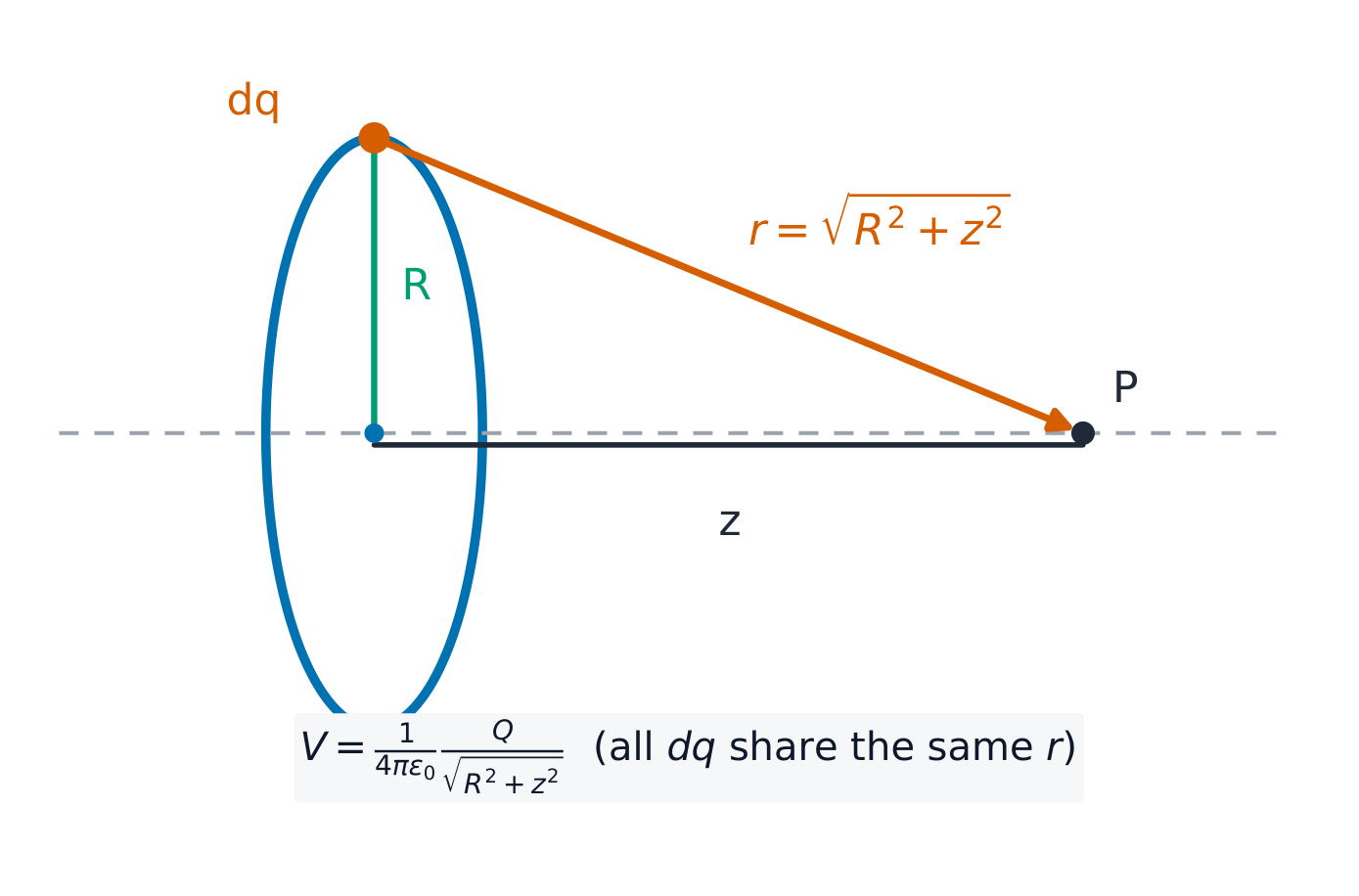
Worked example (ring of charge). A thin ring of radius $R$ carries total charge $Q$. For a point $P$ on the axis a distance $z$ from the centre, every element $dq$ sits at the same distance $r=\sqrt{R^2+z^2}$ from $P$. The distance is constant, so it comes out of the integral:
$$V=\frac{1}{4\pi\varepsilon_0}\int\frac{dq}{\sqrt{R^2+z^2}}=\frac{1}{4\pi\varepsilon_0}\frac{Q}{\sqrt{R^2+z^2}}.$$On an FRQ, say that $r$ is the same for every element – that statement is the marked step. The same idea gives $V=kQ/R$ at the centre of any arc, whatever its angle.
From potential to field
Potential and field contain the same information, linked by a derivative in each direction and by a path integral:
$$E_x=-\frac{dV}{dx},\qquad \Delta V=V_b-V_a=-\int_a^b \vec{E}\cdot d\vec{r}.$$The field is the negative gradient 梯度 of the potential: $\vec{E}$ points from high potential to low potential, "downhill". Where $V$ changes quickly, the field is strong.
Worked example. Along the $x$-axis, $V(x)=3x^{2}-2x$ (volts, with $x$ in metres). Then $E_x=-\dfrac{dV}{dx}=2-6x\ \text{V/m}$. At $x=0.50\ \text{m}$, $E_x=-1.0\ \text{V/m}$: the field there points in the $-x$ direction.
The potential difference 电势差 between two points is the change in potential energy per unit charge moved between them: $\Delta V=\Delta U_E/q$. A battery makes a potential difference chemically: reactions inside separate positive from negative charge and hold the terminals a fixed $\Delta V$ apart.
Equipotential maps
An equipotential 等势面 line (also called an isoline 等值线) joins points that share the same potential. Four rules let you read any map:
- Isolines are perpendicular 垂直 to field lines 电场线 everywhere they cross.
- $\vec{E}$ points from high $V$ to low $V$ – never along an isoline. Moving a charge along an isoline takes no work.
- Closely spaced isolines mean a strong field: $E\approx-\Delta V/\Delta x$.
- You can sketch the field map from an isoline map, and the isoline map from a field map.
Exam skill. Given a map with isolines every $10\ \text{V}$ spaced about $2\ \text{cm}$ apart, estimate $E\approx\dfrac{10}{0.02}=500\ \text{V/m}$, pointing from the higher-value line to the lower one. The work an external agent does moving a charge $q$ slowly from $A$ to $B$ is $W=q(V_B-V_A)$ – the path taken does not matter.
עבריתפוטנציאל חשמלי הוא אנרגיה פוטנציאלית חשמלית ליחידת מטען בנקודה במרחב. הוא נמדד בוולטים ($1\ \text{V}=1\ \text{J/C}$):
$$V=\frac{U_E}{q},\qquad V=\frac{1}{4\pi\varepsilon_0}\frac{q}{r}\ \text{(point charge)}.$$הפוטנציאל הוא סקלרי: יש לו סימן אך אין לו כיוון. הדבר הופך את $V$ לקל הרבה לעיבוד מאשר השדה $\vec{E}$. עבור מספר מטעני נקודה, השתמש ב-סיכום סקלרי – חבר את הפוטנציאלים עם הסימנים שלהם:
$$V=\frac{1}{4\pi\varepsilon_0}\sum_i \frac{q_i}{r_i}.$$דוגמה מפורטת. הפוטנציאל $0.10\ \text{m}$ ממטען נקודה $+3.0\ \text{nC}$ הוא $V=\dfrac{kq}{r}=\dfrac{9.0\times10^{9}(3.0\times10^{-9})}{0.10}=270\ \text{V}$. עכשיו הוסף מטען $-3.0\ \text{nC}$ ב-$0.30\ \text{m}$ מאותה נקודה: הוא תורם $\dfrac{9.0\times10^{9}(-3.0\times10^{-9})}{0.30}=-90\ \text{V}$, ולכן הסך הכל הוא $270-90=180\ \text{V}$. פשוט סכום סימני – אין רכיבי וקטור לפתרון.
חלוקות מטען רציפות
עבור חלוקת מטען רציפה, חלק אותה לחתיכות קטנות $dq$, התעלם בכל חתיכה כמטען נקודה, ואסוף (אינטגרל):
$$V=\frac{1}{4\pi\varepsilon_0}\int\frac{dq}{r}.$$זו אינטגרלת סקלר, ולכן היא בדרך כלל הרבה יותר קלה מאינטגרל השדה. AP מצפה שתדע להתמודד עם ארבעה צורות באמצעות ק্যালקולוס: טבעת דקה (על נקודה בציר שלה), קשת (במרכזה), קו או חוט סופי (בציר הקו, או על האנכים האמצעי שלו), וחוט או צילינדר אינסופיים (על מרחק מהציר שלו).
טבעת מטען: כל אלמנט dq נמצא באותו מרחק מנקודת ציר דוגמה מפורטת (טבעת מטען). טבעת דקה ברדיוס $R$ נושאת מטען כולל $Q$. עבור נקודה $P$ על הציר במרחק $z$ מהמרכז, כל אלמנט $dq$ נמצא באותו מרחק $r=\sqrt{R^2+z^2}$ מ-$P$. המרחק קבוע, ולכן הוא יוצא מהאינטגרל:
$$V=\frac{1}{4\pi\varepsilon_0}\int\frac{dq}{\sqrt{R^2+z^2}}=\frac{1}{4\pi\varepsilon_0}\frac{Q}{\sqrt{R^2+z^2}}.$$בשאלת FRQ, אמור ש-$r$ זהה לכל אלמנט – המשפט הזה הוא השלב הממוקד. אותו רעיון נותן $V=kQ/R$ במרכז כל קשת, לא משנה מה הזווית שלה.
מפוטנציאל לשדה
הפוטנציאל והשדה מכילים את אותו מידע, מקושרים על ידי נגזרת בכל כיוון ועל ידי אינטגרל מסלול:
$$E_x=-\frac{dV}{dx},\qquad \Delta V=V_b-V_a=-\int_a^b \vec{E}\cdot d\vec{r}.$$השדה הוא ה-גרדיאנט השלילי של הפוטנציאל: $\vec{E}$ מצביע מפוטנציאל גבוה לנמוך, "מטה". היכן ש-$V$ משתנה במהירות, השדה חזק.
דוגמה מפורטת. לאורך ציר ה-$x$, $V(x)=3x^{2}-2x$ (וולטים, כאשר ⟨$x$⟩ במטר). אזי $E_x=-\dfrac{dV}{dx}=2-6x\ \text{V/m}$. ב-$x=0.50\ \text{m}$, $E_x=-1.0\ \text{V/m}$: השדה שם מצביע בכיוון ה-$-x$.
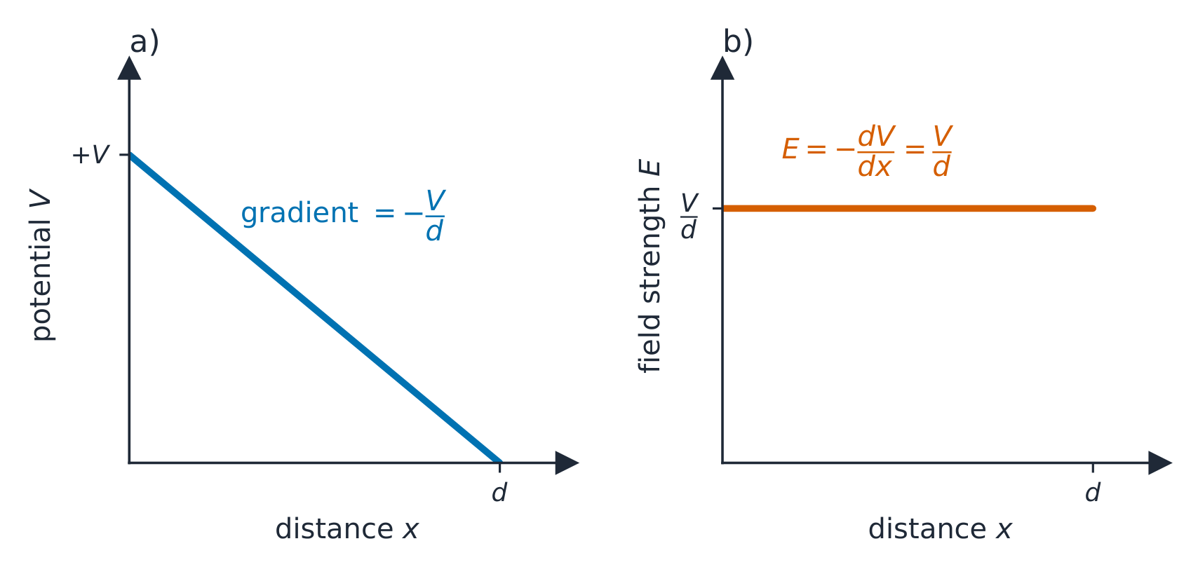
בשדה אחיד הפוטנציאל יורד באופן עקבי עם המרחק הפרש הפוטנציאלים בין שתי נקודות הוא השינוי באנרגיה הפוטנציאלית ליחידת מטען שנע ביןיהן: $\Delta V=\Delta U_E/q$. סוללה יוצרת הפרש פוטנציאלים כימי: תגובות בפנים מפרידות מטען חיובי ממטען שלילי ומחזיקות את המגעים במרחק קבוע ⟨$\Delta V$⟩ אחד מהשני.
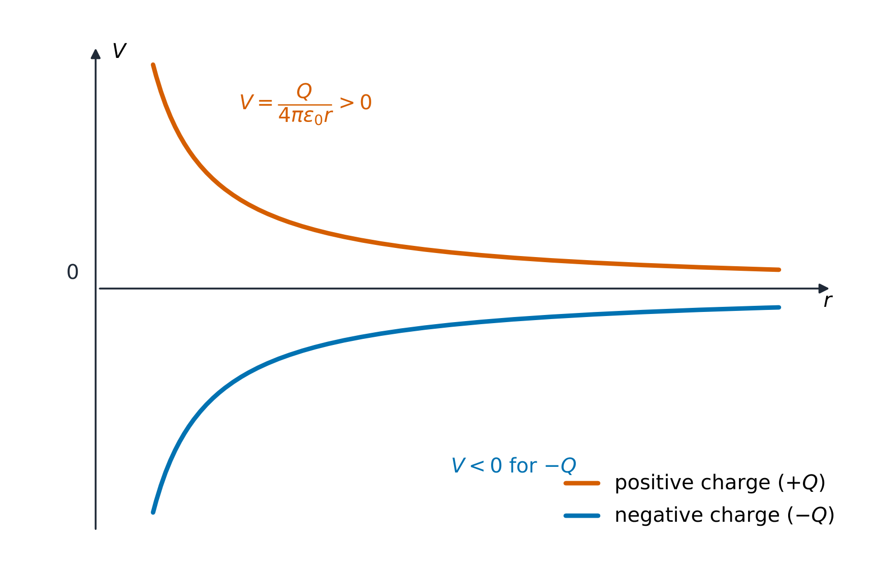
הפוטנציאל סמוך לטען נקודתי משתנה לפי 1/r מפות שטח פוטנציאל
קו שטח פוטנציאל (נקרא גם איזוליין) מחבר נקודות בעלות אותו פוטנציאל. ארבעה כללים מאפשרים לקרוא כל מפה:
- איזולינים הם ניצבים לקווי השדה בכל מקום שבו הם חוצים אותם.
- $\vec{E}$ מצביע מ$V$ גבוה ל$V$ נמוך – לעולם לא לאורך קו מתח. הזזת מטען לאורך קו מתח אינה דורשת עבודה.
- איזולינים צפופים משמעותם שדה חזק: $E\approx-\Delta V/\Delta x$.
- ניתן לשרטט את מפת השדה מתוך מפת איזולינים, ואת מפת האיזולינים מתוך מפת השדה.
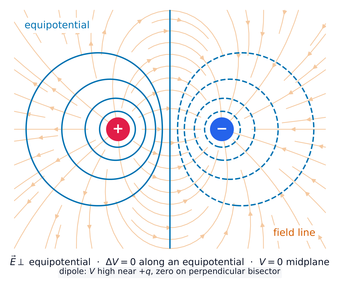
קווי שטח פוטנציאל סביב דופול חוצים את קווי השדה בזווית ישרה כישור מבחן. נתונה מפה עם קווי מתח המרוחקים זה מזה ב-$10\ \text{V}$, הערך הממוצע בין קווים הוא כ-$2\ \text{cm}$. חשב את $E\approx\dfrac{10}{0.02}=500\ \text{V/m}$, שמצביע מהקו בעל הערך הגבוה אל הקו בעל הערך הנמוך. העבודה שבוצעה על ידי גורם חיצוני בהזזת מטען $q$ לאט מ-$A$ ל-$B$ היא $W=q(V_B-V_A)$ – מסלול ההזזה אינו משנה.
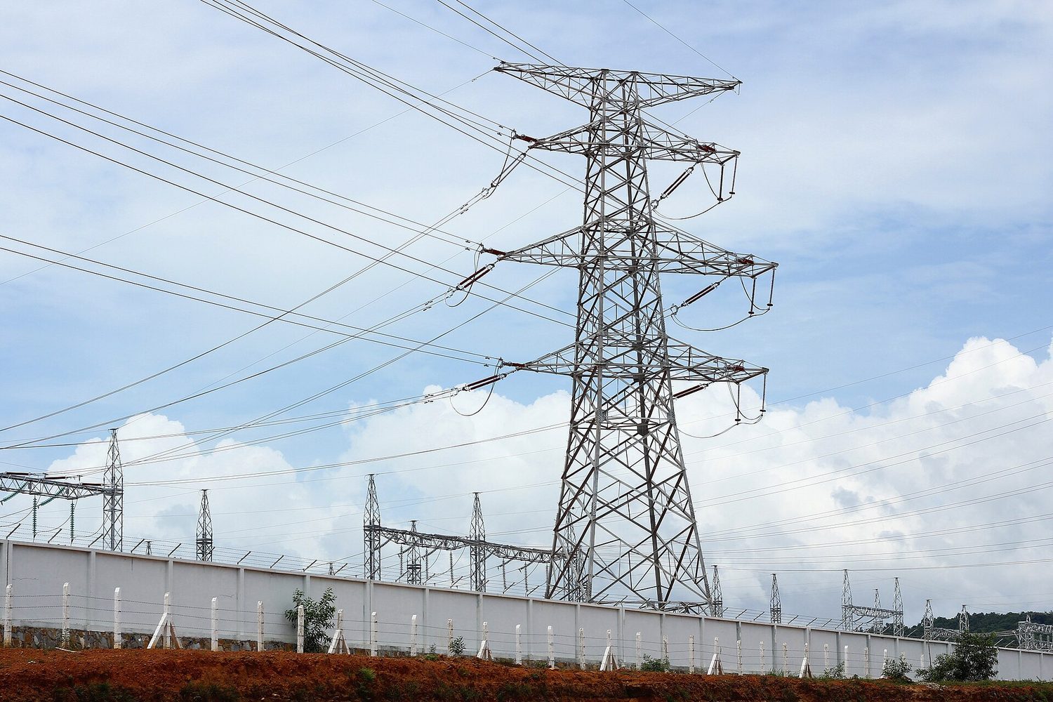
קווי מתח גבוה: אנרגיה פוטנציאלית חשמלית מומרת ומועברת כתורעה במתח גבוה Explore · חקורField lines and the potential around a charge · קווי שדה והפוטנציאל סביב מטען
Electric potential is the energy per unit charge. It falls off with distance from a positive charge; the field lines point from high potential to low. · פוטנציאל חשמלי הוא האנרגיה ליחידת מטען. הוא יורד ככל שהמרחק ממטען חיובי גדל; קווי השדה מכוונים מפוטנציאל גבוה לנמוך.
Vocabulary · מילון מונחים Train · אימוןEnglish עברית work/wɜːk/ עבודה electric potential energy/ɪˈlektrɪk pəˈtenʃl ˈenədʒi/ אנרגיה פוטנציאלית חשמלית kinetic energy/kɪˈnetɪk ˈenədʒi/ אנרגיה קינטית conservative force/kənˈsɜːvətɪv fɔːs/ כוח שמרני system/ˈsɪstəm/ מערכת Electric potential/ɪˈlektrɪk pəˈtenʃl/ פוטנציאל חשמלי scalar/ˈskeɪlə/ סקאלר point charges/pɔɪnt ˈtʃɑːdʒɪz/ טענות נקודתיות superposition/ˌsuːpəpəˈzɪʃn/ הפרעה (סופרפוזיציה) continuous charge distribution/kənˈtɪnjuːəs tʃɑːdʒ ˌdɪstrɪˈbjuːʃn/ חלוקת טענה רציפה integrate/ˈɪntɪɡreɪt/ לאינטגרציה gradient/ˈɡreɪdɪənt/ שיפוע potential difference/pəˈtenʃl ˈdɪfrəns/ הפרש פוטנציאלים equipotential/ˌiːkwɪpəˈtenʃl/ אEquipotential (אי-פוטנציאלי) isoline/ˈaɪsəliːn/ קו איזוליני perpendicular/ˌpɜːpənˈdɪkjʊlə/ ניצב field lines/fiːld laɪnz/ קווי שדה 9.3
Conservation of Electric Energy · שימור אנרגיה חשמלית
Syllabus · סיילבוס
EnglishLearning Objective 9.3.A: Describe changes in a system due to a difference in electric potential between two locations.
- 9.3.A.1 When a charged object moves between two locations with different electric potentials, the resulting change in the electric potential energy of the object-field system is given by the following equation.
- Equation: $\Delta U_E = q\Delta V$
- 9.3.A.2 The movement of a charged object between two points with different electric potentials results in a change in kinetic energy of the object consistent with the conservation of energy.
עבריתמטרות הלמידה 9.3.A: לתאר שינויים במערכת כתוצאה מהפרש בפוטנציאל חשמלי בין שני מיקומים.
- 9.3.A.1 כאשר גוף טעון נע בין שני מיקומים עם פוטנציאלים חשמליים שונים, השינוי הנובע באנרגיה הפוטנציאלית החשמלית של מערכת הגוף-שדה נתון על ידי המשוואה הבאה.
- משוואה: $\Delta U_E = q\Delta V$
- 9.3.A.2 תנועת גוף טעון בין שתי נקודות עם פוטנציאלים חשמליים שונים גורמת לשינוי באנרגיה הקינטית של הגוף תואם לשימור האנרגיה.
Source: College Board AP Course and Exam Description · מקור: תיאור הקורס והמבחן של College Board AP
EnglishWhen a charge $q$ moves between two points that differ in potential by $\Delta V$, the potential energy of the charge–field system changes by
$$\Delta U_E=q\,\Delta V.$$If only the electric force acts, total energy is conserved, so the kinetic energy changes by the opposite amount:
$$\Delta K=-\Delta U_E=-q\,\Delta V.$$Watch the two signs together: a positive charge speeds up when it moves to lower potential, while a negative charge speeds up when it moves to higher potential. Both are just the system trading potential energy for kinetic energy. This is how particle accelerators give charged particles their energy, and it underlies energy analysis in circuits.
Worked example. A proton ($q=1.6\times10^{-19}\ \text{C}$, $m=1.67\times10^{-27}\ \text{kg}$) starts at rest and is accelerated through a potential drop of $500\ \text{V}$ (it moves to lower potential, so $\Delta V=-500\ \text{V}$ and $\Delta K=-q\,\Delta V=+8.0\times10^{-17}\ \text{J}$). Setting $\Delta K=\tfrac12 mv^2$:
$$v=\sqrt{\frac{2(8.0\times10^{-17})}{1.67\times10^{-27}}}=3.1\times10^{5}\ \text{m/s}.$$Exam skill. Choose energy methods, not kinematics, whenever the field is non-uniform or the path curves: only the end-point potentials matter. A typical FRQ chain is $q\,\Delta V \to \Delta K \to v$, with one line of justification: "the electric force is conservative, so energy is conserved."
עבריתכאשר מטען $q$ זז בין שתי נקודות שהפרש הפוטנציאל ביניהן הוא $\Delta V$, האנרגיה הפוטנציאלית של מערכת המטען-שדה משתנה ב-
$$\Delta U_E=q\,\Delta V.$$אם רק הכוח החשמלי פועל, האנרגיה הכוללת שמורה, ולכן האנרגיה הקינטית משתנה בכמות ההפוכה:
$$\Delta K=-\Delta U_E=-q\,\Delta V.$$הסתכלו על שני הסימנים יחד: מטען חיובי מאיץ כאשר הוא זז ל-פוטנציאל נמוך, בעוד שמטען שלילי מאיץ כאשר הוא זז ל-פוטנציאל גבוה. שניהם פשוט מחליפים את האנרגיה הפוטנציאלית באנרגיה קינטית. זוהי הדרך שבה מאיצי חלקיקים מספקים לחלקיקים טעונים אנרגיה, והיא מהווה בסיס לניתוח אנרגטי במעגלים.
דוגמה פתורה. פרוטון ($q=1.6\times10^{-19}\ \text{C}$, $m=1.67\times10^{-27}\ \text{kg}$) מתחיל ממצב רגיעה ומאיץ בשטח פוטנציאל של ⟨$500\ \text{V}$⟩ (הוא זז לפוטנציאל נמוך, ולכן $\Delta V=-500\ \text{V}$ ו-$\Delta K=-q\,\Delta V=+8.0\times10^{-17}\ \text{J}$). נקבע $\Delta K=\tfrac12 mv^2$:
$$v=\sqrt{\frac{2(8.0\times10^{-17})}{1.67\times10^{-27}}}=3.1\times10^{5}\ \text{m/s}.$$כישור למבחן. בחרו בשיטות אנרגטיות ולא בקינמטיקה, כאשר השדה אינו אחיד או שהמסלול מתעקם: רק פוטנציאלי הנקודות הקצה חשובים. שרשרת FRQ אופיינית היא $q\,\Delta V \to \Delta K \to v$, עם שורת נימוק אחת: "הכוח החשמלי הוא שימורי, ולכן האנרגיה שמורה."
9.3
Exam tips · טיפים לבחינות
English- Relate field and potential by $V=-\int \vec E\cdot d\vec l$ and $\vec E=-\nabla V$ (in 1-D, $E_x=-\tfrac{dV}{dx}$).
- Potential is a scalar — add contributions with signs, no vector components needed.
- Potential energy of a pair is $U=\tfrac{1}{4\pi\varepsilon_0}\tfrac{q_1 q_2}{r}$; use energy conservation for a charge's speed.
- Know that no work is done moving along an equipotential, which is perpendicular to $\vec E$.
- Choose the zero of potential (usually infinity) and state it.
עברית- קשר בין שדה לפוטנציאל באמצעות $V=-\int \vec E\cdot d\vec l$ ו$\vec E=-\nabla V$ (ב-1-D, $E_x=-\tfrac{dV}{dx}$).
- פוטנציאל הוא סקלרי – יש להוסיף תרומות עם סימנים, ללא צורך ברכיבי וקטור.
- האנרגיה הפוטנציאלית של זוג היא $U=\tfrac{1}{4\pi\varepsilon_0}\tfrac{q_1 q_2}{r}$; השתמשו בשימור אנרגיה כדי למצוא את מהירותו של מטען.
- לדעת שאין עבודה נעשית בהזזה לאורך שטח פוטנציאל, שהוא ניצב ל-$\vec E$.
- בחר את אפס הפוטנציאל (בדרך כלל אינסוף) וצין אותו.
-
10
Conductors and Capacitors · מוליכים ומכבידים
Watch lesson · צפה בשיעור10.1
Electrostatics with Conductors · אלקטרוסטטיקה עם מוליכים
Syllabus · סיילבוס
Learning Objective Essential Knowledge 10.1.A
Describe the charge distribution within a conductor.- 10.1.A.1 An ideal conductor is a material in which electrons are able to move freely.
- 10.1.A.2 When a conductor is in electrostatic equilibrium, mutual repulsion of excess charge carriers results in those charge carriers residing entirely on the surface of the conductor.
- 10.1.A.2.i In a conductor with a negative net charge, excess electrons reside on the surface of the conductor.
- 10.1.A.2.ii In a conductor with a positive net charge, the surface becomes deficient in electrons, and can be modeled as if positive charge carriers reside on the surface of the conductor.
- 10.1.A.3 Excess charges will move to the surface of a conductor to create a state of electrostatic equilibrium within the conductor.
- 10.1.A.3.i The time interval over which charges reach electrostatic equilibrium within a conductor is so short as to be negligible.
- 10.1.A.3.ii When a conductor reaches electrostatic equilibrium, all points on the surface of the conductor have the same electric potential, and the conductor becomes an equipotential surface.
- 10.1.A.3.iii The charge density on the surface of a conductor will be greater where there are points or edges compared to planar areas.
- 10.1.A.4 All excess charges reside on the surface of a conductor, which means there is no net charge in the interior of the conductor, and the electric field is zero within the conductor.
- 10.1.A.5 The electric field is perpendicular to the outer surface of a conductor.
- 10.1.A.6 A conductor can be polarized in the presence of an external electric field. This is a consequence of the conductor remaining an equipotential surface.
- 10.1.A.7 Electrostatic shielding is the process of surrounding an area with a closed, conducting shell to create a region inside the conductor that is free from external electric fields.
Source: College Board AP Course and Exam Description · מקור: תיאור הקורס והמבחן של College Board AP
EnglishIn an ideal conductor 导体, electrons move freely. Put extra charge on one and the charges repel each other until, almost instantly, they settle into electrostatic equilibrium 静电平衡. In that state the conductor has four properties you must be able to state and use:
- The electric field inside the conductor is zero. If it were not, free electrons would still be moving.
- All excess charge sits on the surface. (Negative net charge = extra electrons on the surface; positive = a shortage of electrons there.)
- The field just outside is perpendicular 垂直 to the surface, with magnitude $E=\sigma/\varepsilon_0$. Any parallel component would push charge sideways along the surface.
- The whole conductor is one equipotential surface 等势面: every point, inside and on the surface, is at the same potential.
Charge density is largest where the surface curves sharply – at points and edges – so the outside field is strongest there. In an external field a conductor polarizes: charge shifts on its surface so that the interior stays field-free and the body stays an equipotential. Surrounding a region with a closed conducting shell keeps outside fields out entirely – electrostatic shielding 静电屏蔽, the idea behind the Faraday cage 法拉第笼.
עבריתבמוליך אידיאלי, אלקטרונים נעים בחופשיות. אם מוסיפים מטען עודף למוליך, המטענים דוחים זה את זה עד שחולף זמן קצר מאוד והם מתקיים איזון אלקטרוסטטי. במצב זה למוליך יש ארבעה מאפיינים שאתה חייב לדעת להגיד ולהשתמש בהם:
- השדה החשמלי בתוך המוליך הוא אפס. אם לא היה כזה, האלקטרונים החופשיים עדיין היו נעים.
- כל המטען העודף יושב על הפני השטח. (מטען נקי שלילי = אלקטרונים נוספים על הפני השטח; חיובי = מחסור באלקטרונים שם.)
- השדה מיד מחוץ לפני השטח הוא ניצב לפני השטח, בעוצמה $E=\sigma/\varepsilon_0$. כל רכיב מקביל לדחיפת מטען בצד לאורך הפני השטח.
- כל המוליך הוא פני פוטנציאל אחיד: כל נקודה, בתוך ובפני השטח, נמצאת באותו פוטנציאל.
צפיפות המטען הגבוהה ביותר היא במקומות שבהם הפני שטח מתכופפים בחריפות – בנקודות ובקצוות – ולכן השדה החיצוני חזק שם ביותר. בשדה חיצוני, מוליך מתקוטב: המטען משתנה בפני השטח כך שהפנים נותר ללא שדה והגוף נשאר פני פוטנציאל אחיד. סביבת אזור עם מעטפת מוליכת סגורה שומרת על שדות חיצוניים מחוץ לחלוטין – הגנה אלקטרוסטטית, הרעיון שעומד מאחורי כלוב פאראדיי.
10.2
Redistribution of Charge Between Conductors · חלוקת מטען בין מוליכים
Syllabus · סיילבוס
EnglishLearning Objective 10.2.A: Describe the movement of charge and the resulting interactions when conductors physically contact each other.
- 10.2.A.1 When conductors are in electrical contact, charges will be redistributed such that the surfaces of each conductor are at the same electric potential.
- 10.2.A.2 Ground is an idealized reference point that has zero electric potential and can absorb or provide an infinite amount of charge without changing its electric potential.
- 10.2.A.3 Charge can be induced on a conductor by grounding the conductor in the presence of an external electric field.
עבריתמטרת הלמידה 10.2.A: לתאר את תנועת המטען והאינטראקציות הנובעות מכך כאשר מוליכים נוגעים זה בזה פיזית.
- 10.2.A.1 כאשר מוליכים במגע חשמלי, מטענים יופצו מחדש כך שפני השטח של כל מוליך יהיו באותו פוטנציאל חשמלי.
- 10.2.A.2 האדמה היא נקודת ייחוס אידיאלית בעלת פוטנציאל חשמלי אפס ויכולה לספוג או לספק כמות אינסופית של מטען ללא שינוי בפוטנציאל החשמלי שלה.
- 10.2.A.3 מטען יכול להיות מושפע (ינדוקציה) על מוליך על ידי חיבורו לאדמה בנוכחות שדה חשמלי חיצוני.
Source: College Board AP Course and Exam Description · מקור: תיאור הקורס והמבחן של College Board AP
EnglishWhen two conductors touch (or are wired together), charge flows between them until both surfaces reach the same potential – that is the stopping condition, not "equal charges". A larger sphere holds more charge at the same potential ($V=kQ/R$), so it takes the larger share.
Worked example. A small sphere of radius $R$ carrying $+6.0\ \mu\text{C}$ touches a distant sphere of radius $2R$, then they separate. Equal potentials require $\dfrac{kq_1}{R}=\dfrac{kq_2}{2R}$, so $q_2=2q_1$. With $q_1+q_2=6.0\ \mu\text{C}$: $q_1=2.0\ \mu\text{C}$ and $q_2=4.0\ \mu\text{C}$.
Ground 接地 is an idealized reference at zero potential that can absorb or supply any amount of charge. Grounding a conductor while an external charge is nearby leaves the conductor with a net induced charge 感应电荷: the external field pushes charge of one sign to ground, and cutting the ground wire before removing the external charge traps the rest.
עבריתכששני מוליכים נוגעים זה בזה (או מחוברים בלולאה), מטען זורם ביניהם עד ששני הפני השטח מגיעים ל-אותו פוטנציאל – זה תנאי עצירת הזרימה, ולא "מטענים שווים". כדור גדול יותר מכיל יותר מטען באותו פוטנציאל ($V=kQ/R$), ולכן הוא לוקח את החלק הגדול יותר.
דוגמה מפורטת. כדור קטן ברדיוס $R$ נושא מטען $+6.0\ \mu\text{C}$ נוגע בכדור רחוק ברדיוס $2R$, ואז הם נפרדים. פוטנציאלים שווים דורשים $\dfrac{kq_1}{R}=\dfrac{kq_2}{2R}$, ולכן $q_2=2q_1$. עם $q_1+q_2=6.0\ \mu\text{C}$: $q_1=2.0\ \mu\text{C}$ ו$q_2=4.0\ \mu\text{C}$.
הארקה היא ייחוס אידיאלי באפס פוטנציאל שיכול לספוג או לספק כל כמות של מטען. הארקת מוליך כאשר מטען חיצוני נמצא בקרבתו משאירה את המוליך עם מטען מושרה נטו: השדה החיצוני דוחה מטען של סימן אחד להארקה, וחיתוך חוט ההארקה לפני הסרת המטען החיצוני לוכד את שאר המטען.
10.3
Capacitors · קבלים
Syllabus · סיילבוס
EnglishLearning Objective 10.3.A: Describe the physical properties of a parallel-plate capacitor.
- 10.3.A.1 A parallel-plate capacitor consists of two separated parallel conducting surfaces that can hold equal amounts of charge with opposite signs.
- 10.3.A.2 Capacitance relates the magnitude of the charge stored on each plate to the electric potential difference created by the separation of those charges.
- Equation: $C = \dfrac{Q}{\Delta V}$
- 10.3.A.2.i The capacitance of a capacitor depends only on the physical properties of the capacitor, such as the capacitor's shape and the material used to separate the plates.
- 10.3.A.2.ii The capacitance of a parallel-plate capacitor is proportional to the area of one of its plates and inversely proportional to the distance between its plates. The constant of proportionality is the product of the dielectric constant, $\kappa$, of the material between the plates and the electric permittivity of free space, $\varepsilon_0$.
- Equation: $C = \dfrac{\kappa \varepsilon_0 A}{d}$
- 10.3.A.3 The electric field between two charged parallel plates with uniformly distributed electric charge, such as in a parallel-plate capacitor, is constant in both magnitude and direction, except near the edges of the plates.
- 10.3.A.3.i The magnitude of the electric field between two charged parallel plates, where the plate separation is much smaller than the dimensions of the plates, can be determined by applying Gauss's law and the principle of superposition.
- Equation: $E = \dfrac{Q}{\varepsilon_0 A}$
- 10.3.A.3.ii The electric field is proportional to the surface charge density on either plate of the capacitor.
- 10.3.A.3.iii A charged particle between two oppositely charged parallel plates undergoes constant acceleration, and therefore its motion shares characteristics with the projectile motion of an object with mass in the gravitational field near Earth's surface.
- 10.3.A.3.i The magnitude of the electric field between two charged parallel plates, where the plate separation is much smaller than the dimensions of the plates, can be determined by applying Gauss's law and the principle of superposition.
- 10.3.A.4 The electric potential energy stored in a capacitor is equal to the work done by an external force to separate that amount of charge on the capacitor.
- 10.3.A.5 The electric potential energy stored in a capacitor is described by the equation $U_C = \dfrac{1}{2} Q \Delta V$.
Boundary statement: While other shapes are also able to separate charges, AP Physics C: Electricity & Magnetism only expects the quantitative analysis and description of parallel-plate capacitors, concentric spherical capacitors, and coaxial cylindrical capacitors.
עבריתמטרת הלמידה 10.3.A: לתאר את התכונות הפיזיקליות של קבל לוחות מקבילים.
- 10.3.A.1 קבל לוחות מקבילים מורכב משתי משטחים מוליכים מקבילים ומרוחקים שמסוגלים להכיל כמויות שוות של מטען עם סימנים מנוגדים.
- 10.3.A.2 הקיבול קובע את הקשר בין גודל המטען המאוחסן בכל לוח לבין הפרש הפוטנציאל החשמלי הנוצר על ידי ההפרדה בין מטענים אלו.
- משוואה: $C = \dfrac{Q}{\Delta V}$
- 10.3.A.2.i הקיבול של קבל תלוי רק בתכונות הפיזיקליות שלו, כגון צורת הקבל והחומר המשמש להפרידה בין הלוחות.
- 10.3.A.2.ii הקיבול של קבל לוחות מקבילים פרופורציונלי לשטח אחד מהלוחות והופך לפרופורציונלי הפוך למרחק בין הלוחות. קבוע הפרופורציונליות הוא מכפלת קבוע הדיאלקטרי, $\kappa$, של החומר שבין הלוחות והאפריטיביות החשמלית של ריק, $\varepsilon_0$.
- משוואה: $C = \dfrac{\kappa \varepsilon_0 A}{d}$
- 10.3.A.3 השדה החשמלי בין שני לוחות מקבילים טעונים עם מטען חשמלי המפוזר באופן אחיד, כגון בקבל לוחות מקבילים, הוא קבוע גם בגודלו וגם בכיוונו, למעט בקרבת קצוות הלוחות.
- 10.3.A.3.i גודל השדה החשמלי בין שני לוחות מקבילים טעונים, כאשר מרחק הלוחות קטן משמעותית מממדי הלוחות, ניתן לחשב באמצעות חוק גאוס ועקרון הסופרפוזיציה.
- משוואה: $E = \dfrac{Q}{\varepsilon_0 A}$
- 10.3.A.3.ii השדה החשמלי פרופורציונלי לצפיפות המטען השטחית על כל לוח מהקבל.
- 10.3.A.3.iii חלקיק טעון בין שני לוחות מקבילים עם מטענים מנוגדים עובר בתאוצה קבועה, ולכן התנועה שלו משתפת מאפיינים עם תנועת הפרציל של גוף בעל מסה בשדה הכבידה בקרבת פני כדור הארץ.
- 10.3.A.3.i גודל השדה החשמלי בין שני לוחות מקבילים טעונים, כאשר מרחק הלוחות קטן משמעותית מממדי הלוחות, ניתן לחשב באמצעות חוק גאוס ועקרון הסופרפוזיציה.
- 10.3.A.4 האנרגיה הפוטנציאלית החשמלית המאוחסנת בקבל שווה לעבודה שנעשתה על ידי כוח חיצוני כדי להפריד כמות זו של מטען על הקבל.
- 10.3.A.5 האנרגיה הפוטנציאלית החשמלית המאוחסנת בקבל מתוארת על ידי המשוואה $U_C = \dfrac{1}{2} Q \Delta V$.
הצהרת גבול: בעוד שצורות אחרות יכולות גם הן להפריד מטענים, AP Physics C: חשמל ומגנטיות דורשת רק ניתוח כמותי ותיאור של קבלים לוחות מקבילים, קבלים כדוריים ממוקדים וקבלים צילינדרים קואקסיאליים.
Source: College Board AP Course and Exam Description · מקור: תיאור הקורס והמבחן של College Board AP
EnglishCharging a capacitor (RC) A capacitor 电容器 stores charge on two conductors separated by a gap: $+Q$ on one plate, $-Q$ on the other. Its capacitance 电容 relates the stored charge to the potential difference between the plates:
$$C=\frac{Q}{\Delta V}.$$Capacitance depends only on geometry and the material in the gap – never on $Q$ or $\Delta V$ themselves.
Worked derivation (parallel plates). For a parallel-plate capacitor 平行板电容器 with plate area $A$ and small gap $d$: Gauss's law plus superposition 叠加 gives a uniform 均匀 field between the plates, $E=\dfrac{\sigma}{\varepsilon_0}=\dfrac{Q}{\varepsilon_0 A}$ (each plate alone contributes $\sigma/2\varepsilon_0$; between the plates the two add, outside they cancel). A uniform field means $\Delta V=Ed=\dfrac{Qd}{\varepsilon_0 A}$, so
$$C=\frac{Q}{\Delta V}=\frac{\varepsilon_0 A}{d}.$$This $E\to\Delta V\to C$ chain is a standard FRQ derivation – learn it as three steps, and quote each one. The same method handles the other two shapes AP expects: concentric spheres ($C=4\pi\varepsilon_0\dfrac{ab}{b-a}$) and a coaxial cylinder of length $L$, where $E=\dfrac{\lambda}{2\pi\varepsilon_0 r}$ gives $\Delta V=\dfrac{\lambda}{2\pi\varepsilon_0}\ln\dfrac{b}{a}$ and so $C=\dfrac{2\pi\varepsilon_0 L}{\ln(b/a)}$.
Worked example. Plates of area $A=0.020\ \text{m}^2$ and gap $d=1.0\ \text{mm}$: $C=\dfrac{8.85\times10^{-12}(0.020)}{1.0\times10^{-3}}=1.8\times10^{-10}\ \text{F}$. Charged to $100\ \text{V}$ it holds $Q=CV=1.8\times10^{-8}\ \text{C}$.
Because the field between the plates is uniform, a charged particle there feels a constant force, so it moves with constant acceleration – exactly like projectile motion 抛体运动 in gravity: constant speed across, uniform acceleration towards a plate.
Worked example. An electron enters midway between plates at $v_0=2.0\times10^{7}\ \text{m/s}$, parallel to them. The field is $E=1.0\times10^{3}\ \text{N/C}$ and the plates are $4.0\ \text{cm}$ long. Acceleration: $a=\dfrac{eE}{m}=\dfrac{(1.6\times10^{-19})(1.0\times10^{3})}{9.11\times10^{-31}}=1.8\times10^{14}\ \text{m/s}^2$. Time between the plates: $t=\dfrac{0.040}{2.0\times10^{7}}=2.0\times10^{-9}\ \text{s}$. Deflection: $y=\tfrac12at^{2}=\tfrac12(1.8\times10^{14})(2.0\times10^{-9})^{2}\approx3.5\times10^{-4}\ \text{m}$ – about $0.35\ \text{mm}$ towards the positive plate.
Storing charge takes work 功: an external force must move each bit of charge against the field of the charge already there. The total work ends up as stored potential energy,
$$U_C=\tfrac12\,Q\,\Delta V=\tfrac12 C(\Delta V)^2=\frac{Q^2}{2C}.$$The factor $\tfrac12$ is the area of the triangle under the $Q$–$\Delta V$ line: the first charge moved across costs almost nothing, the last costs the full $\Delta V$.
Capacitors combine oppositely to resistors: in parallel 并联 the capacitances add ($C_{\text{eq}}=C_1+C_2$, same $\Delta V$, charges add), while in series 串联 the reciprocals add ($\tfrac{1}{C_{\text{eq}}}=\tfrac{1}{C_1}+\tfrac{1}{C_2}$, same $Q$, voltages add).
Worked example. A $2\ \mu\text{F}$ and a $4\ \mu\text{F}$ capacitor in series: $\tfrac{1}{C}=\tfrac12+\tfrac14$, so $C=\tfrac43\ \mu\text{F}$. The same pair in parallel: $6\ \mu\text{F}$.
עבריתטעינת קבל (RC) קבל מאחסן מטען על שני מוליכים המופרדים על ידי רווח: $+Q$ על פלט אחת, $-Q$ על הפלט השנייה. ה-קיבול שלו מקשר את המטען המאוחסן להפרש הפוטנציאל בין הפלטים:
$$C=\frac{Q}{\Delta V}.$$הקיבול תלוי רק בגיאומטריה ובחומר שבמרווח – לעולם לא ב$Q$ או ב$\Delta V$ עצמם.
מסקרת מפורטת (צלעות מקבילות). עבור קבל צלעות מקבילות עם שטח צלעות $A$ ומרווח קטן $d$: חוק גאוס יחד עם סופרפוזיציה נותנו שדה אחיד בין הצלעות, $E=\dfrac{\sigma}{\varepsilon_0}=\dfrac{Q}{\varepsilon_0 A}$ (כל צלע לבדה תורמת $\sigma/2\varepsilon_0$; בין הצלעות שתי התרומות נוספות, מחוץ לצלעות הן מבטלות זו את זו). שדה אחיד פירושו $\Delta V=Ed=\dfrac{Qd}{\varepsilon_0 A}$, ולכן
$$C=\frac{Q}{\Delta V}=\frac{\varepsilon_0 A}{d}.$$שרשרת זו של $E\to\Delta V\to C$ היא מסקרת FRQ סטנדרטית – למד אותה כשלושה שלבים, והסתמך עליהם. אותו שיטה טיפול בשתי הצורות האחרות AP מצפה להן: כדורים ממוקדים ($C=4\pi\varepsilon_0\dfrac{ab}{b-a}$) וצילינדר קואקסיאלי באורך $L$, שבו $E=\dfrac{\lambda}{2\pi\varepsilon_0 r}$ נותן $\Delta V=\dfrac{\lambda}{2\pi\varepsilon_0}\ln\dfrac{b}{a}$ וכך גם $C=\dfrac{2\pi\varepsilon_0 L}{\ln(b/a)}$.
דוגמה מפורטת. צלעות בשטח $A=0.020\ \text{m}^2$ ומרווח $d=1.0\ \text{mm}$: $C=\dfrac{8.85\times10^{-12}(0.020)}{1.0\times10^{-3}}=1.8\times10^{-10}\ \text{F}$. מטעון ל$100\ \text{V}$ הוא מאחסן $Q=CV=1.8\times10^{-8}\ \text{C}$.
מכיוון שהשדה בין הצלעות הוא אחיד, חלקיק טעון שם מרגיש כוח קבוע, ולכן הוא נע עם תאוצה קבועה – בדיוק כמו תנועת פרוגטייל בכבידה: מהירות קבועה אופקית, תאוצה אחידה לכיוון צלע.
חלקיק טעון בין הצלעות נע על פרבולה, כמו פרוגטייל דוגמה פתורה. אלקטרון נכנס במרכז בין לוחות ב$v_0=2.0\times10^{7}\ \text{m/s}$, מקביל אליהם. השדה הוא $E=1.0\times10^{3}\ \text{N/C}$ והלוחות הם $4.0\ \text{cm}$ באורך. האצטות: $a=\dfrac{eE}{m}=\dfrac{(1.6\times10^{-19})(1.0\times10^{3})}{9.11\times10^{-31}}=1.8\times10^{14}\ \text{m/s}^2$. הזמן שבין הלוחות: $t=\dfrac{0.040}{2.0\times10^{7}}=2.0\times10^{-9}\ \text{s}$. הסטייה: $y=\tfrac12at^{2}=\tfrac12(1.8\times10^{14})(2.0\times10^{-9})^{2}\approx3.5\times10^{-4}\ \text{m}$ – כמעט $0.35\ \text{mm}$ כלפי הלוח החיובי.
אחסון מטען דורש עבודה: כוח חיצוני צריך להזיז כל יחידת מטען נגד שדה המטען הקיים. העבודה הכוללת מסתיימת כאנרגיה פוטנציאלית מאוחסנת,
$$U_C=\tfrac12\,Q\,\Delta V=\tfrac12 C(\Delta V)^2=\frac{Q^2}{2C}.$$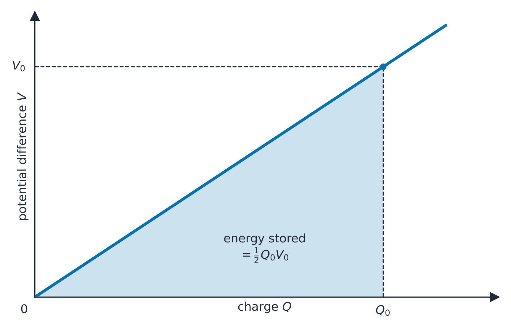
האנרגיה הארוזה בקבל היא השטח מתחת לקו הטעינה-מתח שלו הגורם $\tfrac12$ הוא שטח המשולש מתחת לקו $Q$–$\Delta V$: המטען הראשון שנעבר עלה בעלות זניחה, והאחרון עלה בעלות מלאה של $\Delta V$.
קבלים מחוברים הפוך למנגנונים: במקביל הקבלויות מתחברות ($C_{\text{eq}}=C_1+C_2$, אותו $\Delta V$, המטענים מתחברים), ואילו בסדרה ההפוכים מתחברים ($\tfrac{1}{C_{\text{eq}}}=\tfrac{1}{C_1}+\tfrac{1}{C_2}$, אותו $Q$, המתחים מתחברים).
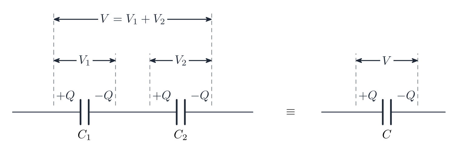
קבלים בסדרה נושאים את אותו מטען, ומתחי הקצה שלהם מתחברים דוגמה פתורה. קבל $2\ \mu\text{F}$ וקבל $4\ \mu\text{F}$ בסדרה: $\tfrac{1}{C}=\tfrac12+\tfrac14$, ולכן $C=\tfrac43\ \mu\text{F}$. אותה זוגיות במקביל: $6\ \mu\text{F}$.
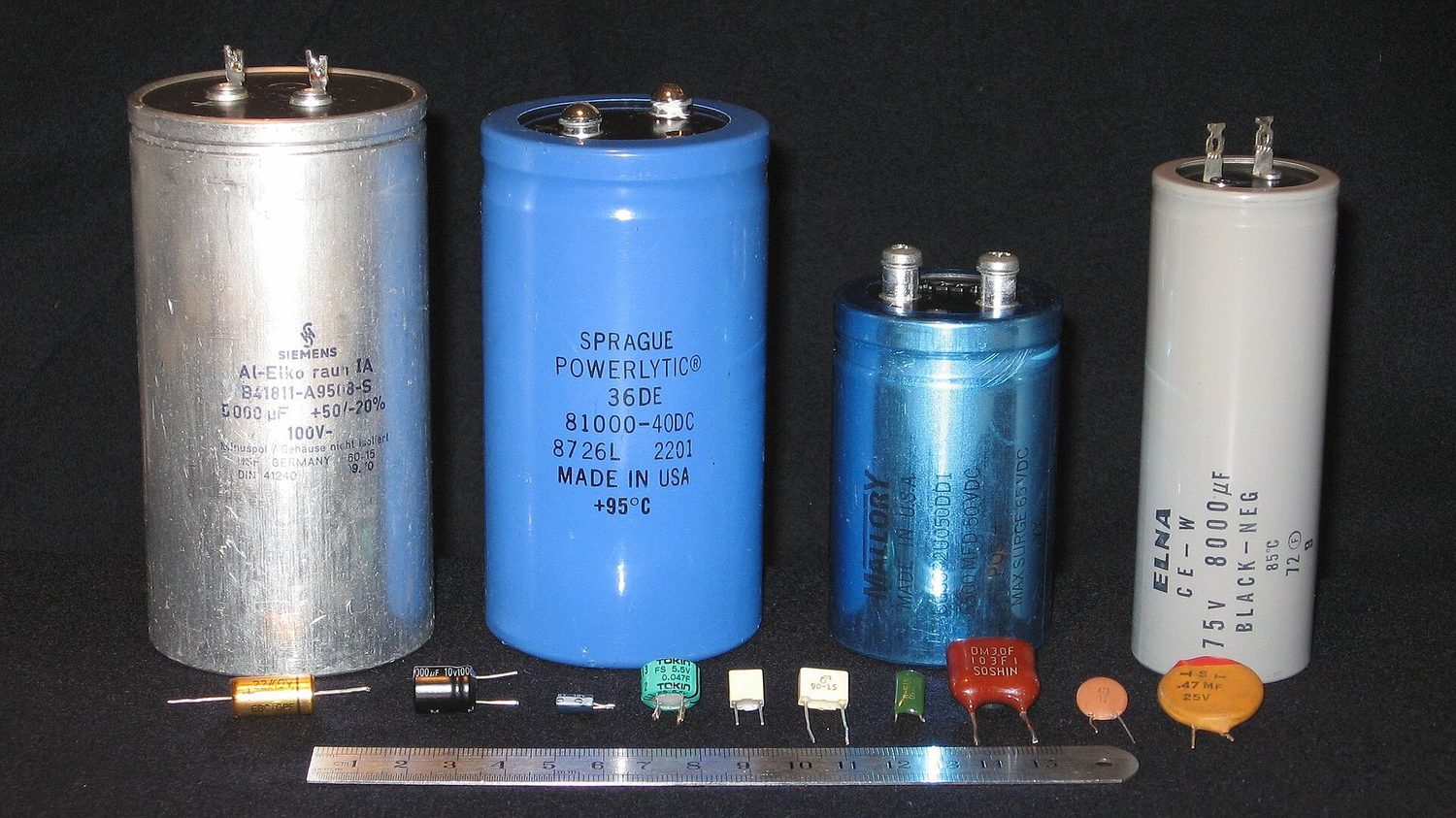
קבלים מגוונים: מכשירים לאחסון מטען ואנרגיה בשדה חשמלי בין מוליכים 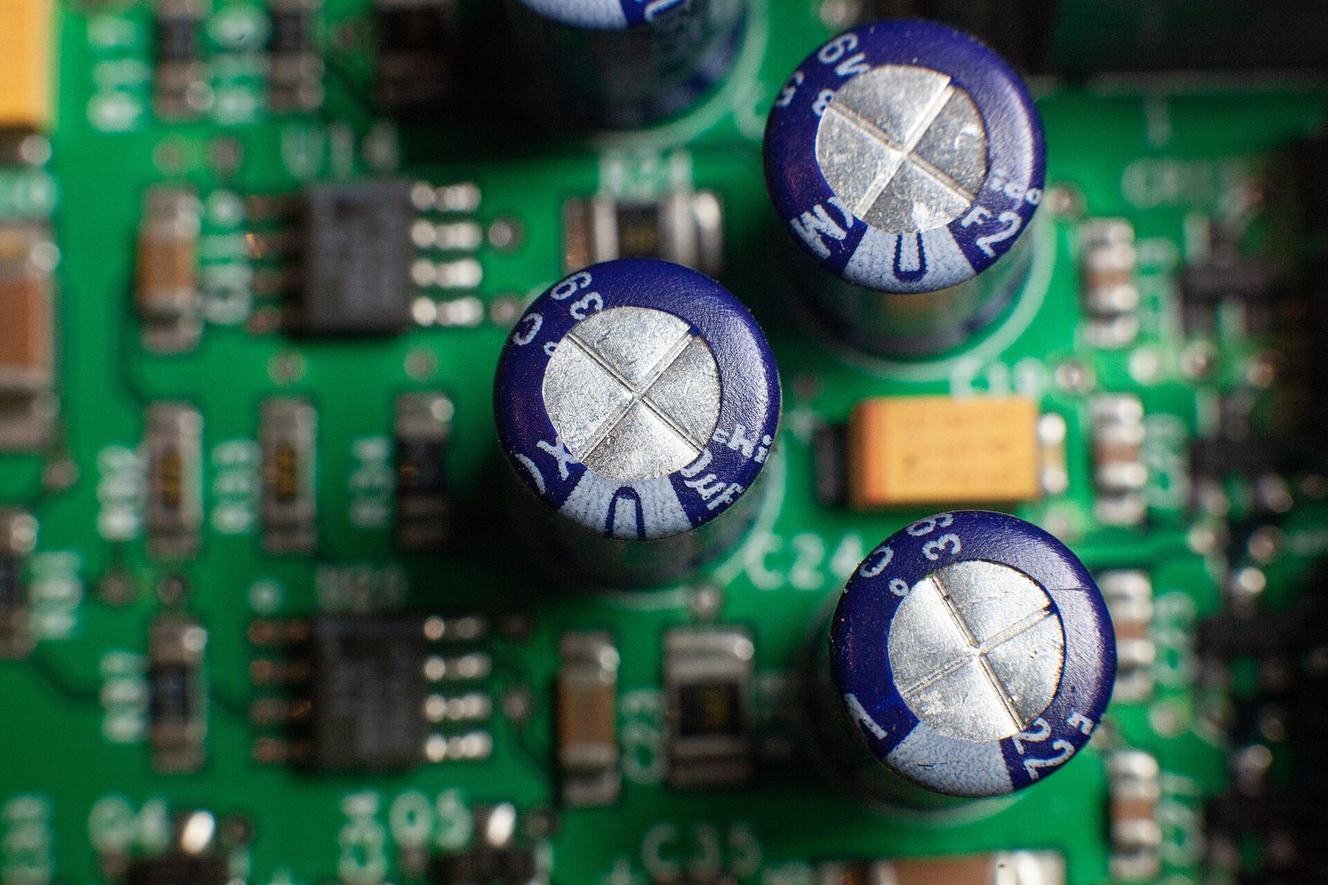
קבלים אלקטרוליטיים על לוח מעגלים: הקבלות אוכרת אנרגיה כ-U = ½CV² Explore · חקורCharge and discharge a capacitor · טעינה ופריקת קבל
A capacitor stores charge on two plates, filling and emptying exponentially with time constant $\tau=RC$. Bigger $R$ or $C$ slows it down. · קבל מאחסן מטען על שני פלאטים, נטען ומתפרק אקספוננציאלית עם זמן-קבוע $\tau=RC$. ערך גדול יותר של $R$ או $C$ מאט את התהליך.
Vocabulary · מילון מונחים Train · אימוןEnglish עברית conductor/kənˈdʌktə/ מו Interructor electrostatic equilibrium/ɪˌlektrəʊˈstætɪk ˌiːkwɪˈlɪbrɪəm/ איזון אלקטרוסטטי perpendicular/ˌpɜːpənˈdɪkjʊlə/ ניצב equipotential surface/ˌiːkwɪpəˈtenʃl ˈsɜːfɪs/ פני שווה-פוטנציאל electrostatic shielding/ɪˌlektrəʊˈstætɪk ˈʃiːldɪŋ/ הגנה אלקסטטית Faraday cage/ˈfærədeɪ keɪdʒ/ כלוב פאראדיי ground/ɡraʊnd/ הארקה induced charge/ɪnˈdjuːst tʃɑːdʒ/ מטען מושרה capacitor/kəˈpæsɪtə/ קבל capacitance/kəˈpæsɪtəns/ קיבול parallel-plate capacitor/ˈpærəlel pleɪt kəˈpæsɪtə/ קבל לוחות מקבילים superposition/ˌsuːpəpəˈzɪʃn/ הפרעה (סופרפוזיציה) uniform/ˈjuːnɪfɔːm/ אחיד projectile motion/prəˈdʒektaɪl ˈməʊʃn/ תנועת פרויקטייל work/wɜːk/ עבודה series/ˈsɪəriːz/ סדרתי 10.4
Dielectrics · דיאלקטרקים

Syllabus · סיילבוס
EnglishLearning Objective 10.4.A: Describe how a dielectric inserted between the plates of a capacitor changes the properties of the capacitor.
- 10.4.A.1 In a dielectric material, electric charges are not as free to move as they are in a conductor. Instead, the material becomes polarized in the presence of an external electric field.
- 10.4.A.2 The dielectric constant of a material relates the electric permittivity of that material to the permittivity of free space.
- Equation: $\kappa = \dfrac{\varepsilon}{\varepsilon_0}$
- 10.4.A.3 The electric field created by a polarized dielectric is opposite in direction to the external field.
- 10.4.A.4 The electric field between the plates of an isolated parallel-plate capacitor decreases when a dielectric is placed between the plates.
- Equation: $\kappa = \dfrac{E_0}{E}$
- 10.4.A.5 The insertion of a dielectric into a capacitor may change the capacitance of the capacitor.
- Equation: $C = \kappa C_0$
עבריתמטרת הלמידה 10.4.A: לתאר כיצד הכנסת דיאלקטריקה בין לוחות הקבל משנה את תכונות הקבל.
- 10.4.A.1 בחומר דיאלקטרי, מטענים חשמליים אינם חופשיים לנוע כמו שהם במוליך. במקום זאת, החומר הופך לפולריזציה בנוכחות שדה חשמלי חיצוני.
- 10.4.A.2 הקבוע הדיאלקטרי של חומר מקשר את הקיבולת החשמלית (האפסיילון) של החומר לקיבולת החשמלית של הרווח.
- משוואה: $\kappa = \dfrac{\varepsilon}{\varepsilon_0}$
- 10.4.A.3 השדה החשמלי שנוצר על ידי דיאלקטרי פולריזציה הוא נגד לכיוון השדה החיצוני.
- 10.4.A.4 השדה החשמלי בין לוחות קבל-מטען מקביל מבודד מצטמצם כאשר מוחדר ביניהם דיאלקטרי.
- משוואה: $\kappa = \dfrac{E_0}{E}$
- 10.4.A.5 הכנסת דיאלקטרי לתוך קבל עשויה לשנות את הקיבולת שלו.
- משוואה: $C = \kappa C_0$
Source: College Board AP Course and Exam Description · מקור: תיאור הקורס והמבחן של College Board AP
EnglishA dielectric 电介质 is an insulating material. Its charges cannot travel, but in an external field each molecule stretches or turns slightly – the material becomes polarized 极化. The lined-up molecules create their own small field opposite to the applied one, so the net field inside the material drops:
$$E=\frac{E_0}{\kappa},\qquad \kappa=\frac{\varepsilon}{\varepsilon_0}\ \ (\kappa>1),$$where $\kappa$ is the dielectric constant 介电常数, the ratio of the material's permittivity to the permittivity of free space 真空介电常数.
Filling a capacitor with dielectric multiplies its capacitance:
$$C=\kappa\,C_0\qquad\left(\text{parallel plates: } C=\frac{\kappa\varepsilon_0 A}{d}\right).$$What happens next depends on what stays fixed – a favourite exam trap:
battery stays connected ($\Delta V$ fixed) battery removed first ($Q$ fixed) charge $Q$ rises to $\kappa Q_0$ unchanged voltage $\Delta V$ unchanged drops to $\Delta V_0/\kappa$ field $E$ unchanged drops to $E_0/\kappa$ energy $U$ rises to $\kappa U_0$ drops to $U_0/\kappa$ Worked example. A $100\ \text{pF}$ capacitor is charged to $12\ \text{V}$, disconnected, then filled with a $\kappa=3$ dielectric. $Q$ is trapped, so $\Delta V$ falls to $4\ \text{V}$ and the stored energy falls to one-third – the missing energy went into pulling the dielectric in. Reconnected to the $12\ \text{V}$ battery instead, the capacitor would hold three times the charge and three times the energy.
Exam skill. Always begin dielectric questions by writing down which quantity is held fixed ($Q$ or $\Delta V$), then let $C=\kappa C_0$ drive everything else through $Q=C\Delta V$ and $U=\tfrac12 C(\Delta V)^2$.
עבריתדיאלקטרק הוא חומר מבודד. המטענים בו אינם יכולים לנוע, אך בשדה חיצוני כל מולקולה נמתחת או מסתובבת מעט – החומר הופך למקוטב. המולקולות המיושרות יוצרות שדה קטן משלהן נגד השדה המופעל, כך שהשדה הנקי בתוך החומר יורד:
$$E=\frac{E_0}{\kappa},\qquad \kappa=\frac{\varepsilon}{\varepsilon_0}\ \ (\kappa>1),$$כאשר $\kappa$ הוא קבוע הדיאלקטרק, היחס בין קבוע הדיאלקטרק של החומר לבין קבוע הדיאלקטרק של ריק.
דיאלקטרק מקוטב יוצר שדה פנימי המנוגד לשדה המופעל מילוי קבל בדיאלקטרק מכפיל את הקבלות שלו:
$$C=\kappa\,C_0\qquad\left(\text{parallel plates: } C=\frac{\kappa\varepsilon_0 A}{d}\right).$$מה שקורה בהמשך תלוי ב מה שנשאר קבוע – כמעצר ב Exam נפוץ:
הסוללה מחוברת ($\Delta V$ קבוע) הסוללה מופרדת תחילה ($Q$ קבוע) מטען $Q$ עולה ל$\kappa Q_0$ אינו משתנה מתח $\Delta V$ אינו משתנה יורד ל$\Delta V_0/\kappa$ שדה $E$ אינו משתנה יורד ל$E_0/\kappa$ אנרגיה $U$ עולה ל$\kappa U_0$ יורדת ל$U_0/\kappa$ דוגמה מודגמת. קבלן $100\ \text{pF}$ נטען ל$12\ \text{V}$, נתקע, ואז מלא בדיאלקטריק $\kappa=3$. $Q$ נכלא, ולכן $\Delta V$ יורד ל$4\ \text{V}$ והאנרגיה האגורה יורד לשליש – האנרגיה החסרה הלכה למשיכת הדיאלקטריק פנימה. מחובר מחדש לסוללה $12\ \text{V}$ במקום זאת, הקבלן יכיל שלוש פעמים יותר מטען ושלוש פעמים יותר אנרגיה.
מיומנות מבחן. תמיד התחל שאלות דיאלקטריק בכתיבה מהכמות הנשמרת קבועה ($Q$ או $\Delta V$), ואז תן ל$C=\kappa C_0$ להניע הכל שאר דרך $Q=C\Delta V$ ו$U=\tfrac12 C(\Delta V)^2$.
Explore · חקורAdd a dielectric · הוסף דיאלקטרי
A dielectric between the plates raises the capacitance, so the capacitor holds more charge at the same voltage. Watch the charge build faster. · דיאלקטרית בין הפלאטים מגבירה את הקיבול, כך שהקבל שומר יותר מטען באותו מתח. שימו לב למטען שנצבר מהר יותר.
Vocabulary · מילון מונחים Train · אימוןEnglish עברית parallel/ˈpærəlel/ מקביל dielectric/ˌdaɪɪˈlektrɪk/ דיאלקטרית polarized/ˈpəʊləraɪzd/ ממוסל dielectric constant/ˌdaɪɪˈlektrɪk ˈkɒnstənt/ קבוע דיאלקטרי permittivity of free space/ˌpɜːmɪˈtɪvəti ɒv friː speɪs/ הפרמיטיביות של ריק 10.4
Exam tips · טיפים לבחינות
English- In electrostatic equilibrium a conductor has $\vec E=0$ inside and all excess charge on the surface.
- Apply Gauss's law $\oint \vec E\cdot d\vec A=\tfrac{q_{enc}}{\varepsilon_0}$ with a symmetry-matched Gaussian surface (sphere, cylinder, pillbox).
- The whole conductor is one equipotential, and the surface field is perpendicular to it.
- For a capacitor use $C=\tfrac{Q}{V}$, energy $U=\tfrac12 CV^2$, and how a dielectric raises $C$.
- Pick the Gaussian surface so $\vec E$ is constant and parallel (or zero) on each part.
עברית- בשיווי משקל אלקטרוסטטי למוליך יש $\vec E=0$ בתוך וכל המטען העודף על הפני.
- יישם אתחוק גאוס $\oint \vec E\cdot d\vec A=\tfrac{q_{enc}}{\varepsilon_0}$ עם פני גאוס המתאימים לסימטריה (כדור, צילינדר, קופסת טabliya).
- כל המוליך הוא איזו-פוטנציאל אחד, ושדה המשטח מאונך אליו.
- עבור קבלן השתמש ב$C=\tfrac{Q}{V}$, אנרגיה $U=\tfrac12 CV^2$, וכיצה דיאלקטריק מעלה $C$.
- בחר את פני גאוס כך ש$\vec E$ יהיה קבוע ומקביל (או אפס) בכל חלק.
-
11
Electric Circuits · מעגלים חשמליים
Watch lesson · צפה בשיעור11.1
Electric Current
Syllabus · סיילבוס
EnglishLearning Objective 11.1.A: Describe the movement of electric charges through a medium.
- 11.1.A.1 Current is the rate at which charge passes through a cross-sectional area of a wire.
- Equation: $I = \dfrac{dq}{dt}$
- 11.1.A.1.i Current within a conductor consists of charge carriers traveling through the conductor with an average drift velocity.
- Equation: $I = nqv_d A$
- 11.1.A.1.ii Electric charge moves in a circuit in response to an electric potential difference, sometimes referred to as electromotive force, or $\mathrm{emf}$ ($\mathcal{E}$).
- 11.1.A.1.iii If the current is zero in a section of wire, the net motion of charge carriers in the wire is also zero, although individual charge carriers will not have zero speed.
- 11.1.A.2 Current density is the flow of charge per unit area.
- Equation: $I = \int \vec{J} \cdot d\vec{A}$
- 11.1.A.2.i Current density is related to the motion of the charge carriers within a conductor.
- Equation: $\vec{J} = nq\vec{v}_d$
- 11.1.A.2.ii Current density is a vector quantity.
- 11.1.A.2.iii A potential difference across a conductor creates an electric field within the conductor that is proportional to the resistivity of the conductor and the current density.
- Equation: $\vec{E} = \rho\vec{J}$
- 11.1.A.3 If a function of current density is given, the total current can be determined by integrating the current density over the area.
- Equation: $I_{\text{tot}} = \int \vec{J}(r) \cdot d\vec{A}$
- 11.1.A.4 Although current is a scalar quantity, it does have a direction. Because its direction is relative to the current carrier and not space, current does not obey the laws of vector addition and has no vector components.
- 11.1.A.4.i The direction of conventional current is chosen to be the direction in which positive charge would move.
- 11.1.A.4.ii In common circuits, the current is actually due to the movement of electrons (negative charge carriers).
עבריתמטרת למידה 11.1.A: לתאר את תנועת מטענים חשמליים דרך תווך.
- 11.1.A.1 זרם הוא הקצב שעבורו מטען עובר דרך שטח חתך של חוט.
- משוואה: $I = \dfrac{dq}{dt}$
- 11.1.A.1.i הזרם בתוך מוליך מורכב ממטענים נעים דרך המוליך עם מהירות נדיפה ממוצעת.
- משוואה: $I = nqv_d A$
- 11.1.A.1.ii מטען חשמלי זז במעגל כתוצאה מפער פוטנציאל חשמלי, הנקרא לעיתים כוח אלקטרומניטיבי או $\mathrm{emf}$ ($\mathcal{E}$).
- 11.1.A.1.iii אם הזרם באזור מסוים של חוט הוא אפס, התנועה הכוללת של נשאי המטען בחוט היא גם כן אפס, למרות שהמהירות של כל נשי מטען בודד אינה אפס.
- 11.1.A.2 צפיפות הזרם היא זרימת המטען ליחידת שטח.
- משוואה: $I = \int \vec{J} \cdot d\vec{A}$
- 11.1.A.2.i צפיפות הזרם קשורה לתנועת נשאי המטען בתוך מוליך.
- משוואה: $\vec{J} = nq\vec{v}_d$
- 11.1.A.2.ii צפיפות הזרם היא גודל וקטורי.
- 11.1.A.2.iii פער פוטנציאל על פני מוליך יוצר שדה חשמלי בתוכו הפרופורציונלי להתנגדות הסגולית של המוליך ולצפיפות הזרם.
- משוואה: $\vec{E} = \rho\vec{J}$
- 11.1.A.3 אם נתונה פונקציה של צפיפות זרם, ניתן לחשב את הזרם הכולל על ידי אינטגרציה של צפיפות הזרם לאורך השטח.
- משוואה: $I_{\text{tot}} = \int \vec{J}(r) \cdot d\vec{A}$
- 11.1.A.4 למרות שהזרם הוא גודל סקלארי, יש לו כיוון. מכיוון שהכיוון שלו תלוי בנשי המטען ולא במרחב, הזרם אינו עומד בחוקי חיבור וקטורים ואין לו רכיבי וקטור.
- 11.1.A.4.i הכיוון של הזרם המקובל נבחר להיות הכיוון בו יזוז מטען חיובי.
- 11.1.A.4.ii במעגלים רגילים, הזרם בפועל נובע מתנועת אלקטרונים (נשי מטען שליליים).
Source: College Board AP Course and Exam Description · מקור: תיאור הקורס והמבחן של College Board AP
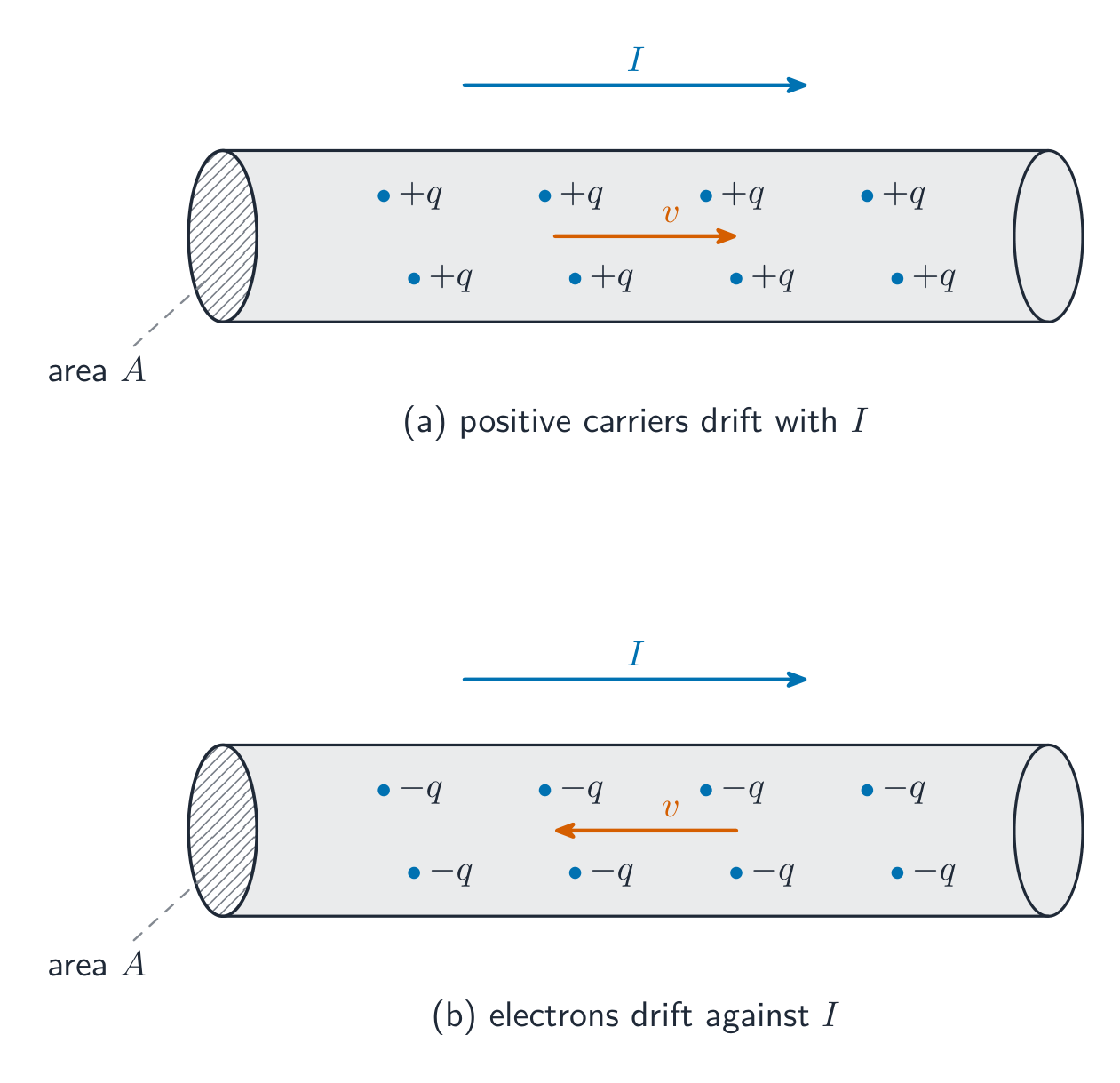
Electric current 电流 is the rate at which charge passes a cross-section of wire, $I=\dfrac{dq}{dt}$, measured in amperes 安培. Conventional current points the way positive charge would move. Microscopically, a current is a slow drift of many carriers:
$$I=nqv_dA,$$with $n$ the number of carriers per volume, $q$ the charge each carries, $v_d$ the drift velocity 漂移速度, and $A$ the cross-sectional area 横截面积.
Charge carriers drift slowly through a conductor to make a current Worked example. A copper wire with $A=1.0\times10^{-6}\ \text{m}^2$ and $n=8.5\times10^{28}\ \text{m}^{-3}$ carries $1.7\ \text{A}$. Then $v_d=\dfrac{I}{nqA}=\dfrac{1.7}{(8.5\times10^{28})(1.6\times10^{-19})(1.0\times10^{-6})}\approx1.3\times10^{-4}\ \text{m/s}$ – the carriers drift slower than a snail, even though the signal travels near light speed.
Current density 电流密度 is charge flow per unit area, $\vec{J}=nq\vec{v}_d$, linked to the field driving it by $\vec{E}=\rho\vec{J}$. In general $I=\int\vec{J}\cdot d\vec{A}$; if $J(r)$ varies across the wire, integrate it over the cross-section to get the total current. One care point: current has a direction along its wire, but it is a scalar 标量 – currents do not add as vectors, and there are no "components of current".
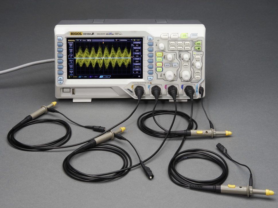
An oscilloscope: voltage against time reveals how current and charge evolve in a circuit Vocabulary · מילון מונחים Train · אימוןEnglish עברית Electric current/ɪˈlektrɪk ˈkʌrənt/ זרם חשמלי amperes/ˈæmpeəz/ אמפרים drift velocity/drɪft vəˈlɒsɪti/ מהירות סחיפה cross-sectional area/krɒs ˈsekʃənl ˈeərɪə/ שטח חתך רוחב Current density/ˈkʌrənt ˈdensɪti/ צפיפות זרם scalar/ˈskeɪlə/ סקאלר 11.2
Electric Circuits
Syllabus · סיילבוס
EnglishLearning Objective 11.2.A: Describe the behavior of a circuit.
- 11.2.A.1 A circuit is composed of electrical loops, which can include wires, batteries, resistors, lightbulbs, capacitors, inductors, switches, ammeters, and voltmeters.
- 11.2.A.2 A closed electrical loop is a closed path through which charges may flow.
- 11.2.A.2.i A closed circuit is one in which charges would be able to flow.
- 11.2.A.2.ii An open circuit is one in which charges would not be able to flow.
- 11.2.A.2.iii A short circuit is one in which charges would be able to flow with no change in potential difference.
- 11.2.A.3 A single circuit element may be part of multiple electrical loops.
- 11.2.A.4 Circuit schematics are representations used to describe and analyze electric circuits.
- 11.2.A.4.i The properties of an electric circuit are dependent on the physical arrangement of its constituent elements.
- 11.2.A.4.ii Circuit elements have common symbols that are used to create schematic diagrams. Variable elements are indicated by a diagonal strikethrough arrow across the standard symbol for that element. (Symbols: Battery, Bulb, Switch, Capacitor, Resistor, Ammeter, Voltmeter, Inductor.)
Boundary statement: Unless otherwise specified, all circuit schematic diagrams will be drawn using conventional current.
עבריתמטרת למידה 11.2.A: לתאר את התנהגותו של מעגל חשמלי.
- 11.2.A.1 מעגל חשמלי מורכב מלולאות חשמליות, שעלולות לכלול חוטים, סוללות, נגדים, נורות, קבלים, סלילי השראה, מתגים, אמפרמטרים ווולטמטרים.
- 11.2.A.2 מעגל חשמלי סגור הוא מסלול סגור דרכו מטענים יכולים לזרום.
- 11.2.A.2.i מעגל סגור הוא אחד שבו מטענים היו יכולים לזרום.
- 11.2.A.2.ii מעגל פתוח הוא אחד שבו מטענים לא היו יכולים לזרום.
- 11.2.A.2.iii קצר חשמלי הוא מצב שבו מטענים יוכלו לזרום ללא שינוי בהפרש הפוטנציאל.
- 11.2.A.3 אלמנט מעגל אחד עשוי להיות חלק ממספר לולאות חשמליות.
- 11.2.A.4 תרשימי מעגלים הם נציגים המשמשים לתאר ולנתח מעגלים חשמליים.
- 11.2.A.4.i המאפיינים של מעגל חשמלי תלויים בסידור הפיזי של האלמנטים המרכיבים אותו.
- 11.2.A.4.ii רכיבי מעגל הם בעלי סמלים סטנדרטיים המשמשים ליצירת סכמות חשמליות. רכיבים משתנים מסומנים על ידי חץ אלכסוני חוצה את הסמל הסטנדרטי של הרכיב. (סמלים: סוללה, נורה, מתג, קבל, נגד, אמפרמטר, וולטמטר, סליל השראה.)
הצהרת גבול: אלא אם כן צוין אחרת, כל תרשימי המעגלים יצורו באמצעות זרם קונבנציונלי.
Source: College Board AP Course and Exam Description · מקור: תיאור הקורס והמבחן של College Board AP
A circuit is a set of closed loops built from wires, batteries, resistors, lightbulbs, capacitors, inductors, switches, and meters; charge can flow only around a closed path. One element can belong to several loops at once – that is what makes multi-loop problems interesting. Every analysis starts by reading the circuit diagram 电路图: trace each loop and identify which elements share the same current (series 串联) and which share the same potential difference (parallel 并联).
Explore · חקורBuild series and parallel circuits · בנה מעגלים בסדר ובמקביל
In series the same current flows through every bulb and voltage divides; in parallel each branch gets the full voltage. Switch mode to see the bulbs' brightness change. · בסדר, אותה עוצמה זורמת דרך כל נורה והמתח מתחלק; במקביל, לכל ענף מגיע המתח המלא. החלף מצב כדי לראות כיצד בהירות הנורות משתנה.
Vocabulary · מילון מונחים Train · אימוןEnglish עברית circuit diagram/ˈsɜːkɪt ˈdaɪəɡræm/ תרשים מעגל חשמלי series/ˈsɪəriːz/ סדרתי parallel/ˈpærəlel/ מקביל 11.3
Resistance, Resistivity, and Ohm's Law
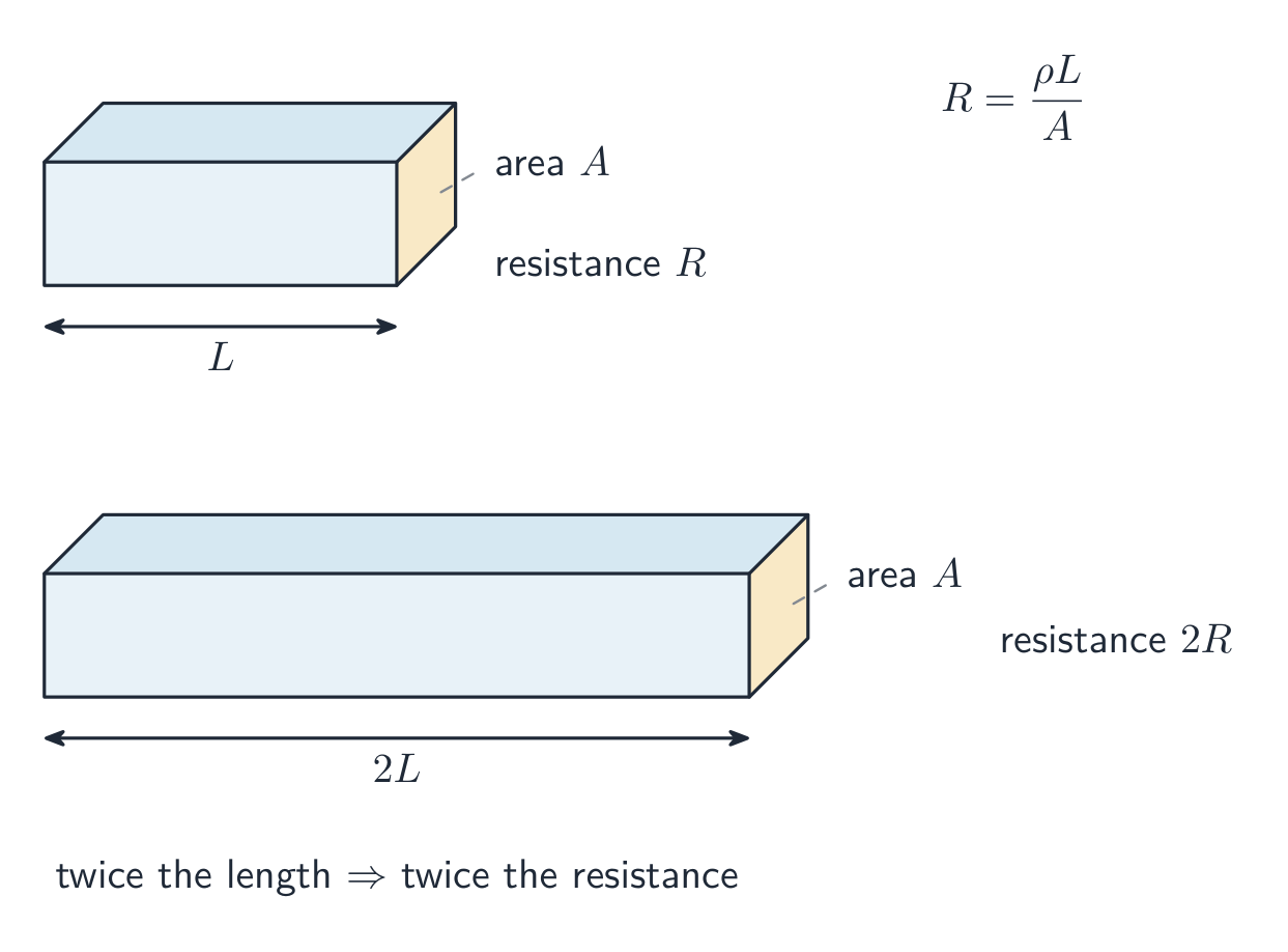
Syllabus · סיילבוס
EnglishLearning Objective 11.3.A: Describe the resistance of an object using physical properties of that object.
- 11.3.A.1 Resistance is a measure of the degree to which an object opposes the movement of electric charge.
- 11.3.A.2 The resistance of a resistor with uniform geometry is proportional to its resistivity and length and is inversely proportional to its cross-sectional area.
- Equation: $R = \dfrac{\rho\ell}{A}$
- 11.3.A.2.i Resistivity is a fundamental property of a material that depends on its atomic and molecular structure and quantifies how strongly the material opposes the motion of electric charge.
- 11.3.A.2.ii The resistivity of a conductor typically increases with temperature.
- 11.3.A.2.iii The total resistance of a resistor with uniform geometry, but that is made of a material whose resistivity varies along the length of the resistor, is given by $R = \int \dfrac{\rho(\ell)\,d\ell}{A}$.
Learning Objective 11.3.B: Describe the electrical characteristics of elements of a circuit.
- 11.3.B.1 Ohm's law relates current, resistance, and potential difference across a conductive element of a circuit.
- Equation: $I = \dfrac{\Delta V}{R}$
- 11.3.B.1.i Materials that obey Ohm's law have constant resistance for all currents and are called ohmic materials.
- 11.3.B.1.ii The resistivity of an ohmic material is constant regardless of temperature.
- 11.3.B.1.iii Resistors can also convert electrical energy to thermal energy, which may change the temperature of both the resistor and the resistor's environment.
- 11.3.B.1.iv The resistance of an ohmic circuit element can be determined from the slope of a graph of the current in the element as a function of the potential difference across the element.
עבריתמטרה לימודית 11.3.A: לתאר את ההתנגדות של חפץ באמצעות מאפיינים פיזיקליים שלו.
- 11.3.A.1 התנגדות היא מדד לדרגה שבה חפץ מונע את תנועת המטען החשמלי.
- 11.3.A.2 ההתנגדות של נגד בעל גיאומטריה אחידה פרופורציונלית להתנגדות הסגולית ולאורכו, והופכת פרופורציונלית לשטח החתך שלו.
- משוואה: $R = \dfrac{\rho\ell}{A}$
- 11.3.A.2.i התנגדות סגולית היא מאפיין בסיסי של חומר התלוי במבנה האטומי והמולקולרי שלו ומכמת עד כמה החומר מונע תנועת מטען חשמלי.
- 11.3.A.2.ii ההתנגדות הסגולית של מוליך עולה לרוב עם הטמפרטורה.
- 11.3.A.2.iii ההתנגדות הכוללת של נגד בעל גיאומטריה אחידה אך העשוי מחומר whose התנגדות הסגולית משתנה לאורך אורך הנגד, נתונה על ידי $R = \int \dfrac{\rho(\ell)\,d\ell}{A}$.
מטרה לימודית 11.3.B: לתאר את המאפיינים החשמליים של אלמנטים במעגל.
- 11.3.B.1 חוק אוהם מקשר בין זרם, התנגדות והפרש פוטנציאל על פני אלמנט מוליך במעגל.
- משוואה: $I = \dfrac{\Delta V}{R}$
- 11.3.B.1.i חומרים העומדים בחוק אוהם בעלי התנגדות קבועה לכל הזרמים ונקראים חומרים אוםיים.
- 11.3.B.1.ii ההתנגדות הסגולית של חומר אומי קבועה ללא קשר לטמפרטורה.
- 11.3.B.1.iii נגדים יכולים גם להמיר אנרגיה חשמלית לאנרגיה תרמית, מה שעשוי לשנות את טמפרטורת הנגד ואת הסביבה סביבו.
- 11.3.B.1.iv ההתנגדות של אלמנט מעגל אומי ניתן לקבוע מהשיפוע של גרף הזרם באלמנט כתפקוד הפרש הפוטנציאל על פניו.
Source: College Board AP Course and Exam Description · מקור: תיאור הקורס והמבחן של College Board AP
Resistance 电阻 measures how strongly an object opposes charge flow. It grows with the material's resistivity 电阻率 and the conductor's length, and shrinks with its area:
$$R=\frac{\rho\,\ell}{A}.$$Ohm's law 欧姆定律 relates the current through an element to the potential difference across it:
$$I=\frac{\Delta V}{R}.$$A longer conductor has more resistance; a wider one has less Worked example. Stretch a wire to double its length: the volume is fixed, so the area halves, and $R=\rho\ell/A$ becomes $\rho(2\ell)/(A/2)=4R$ – four times the resistance. An element is ohmic 欧姆性 if $R$ stays constant (a straight line through the origin on an $I$–$\Delta V$ graph); a lightbulb filament, which heats up, is not.
Explore · חקורApply Ohm's law · החל את חוק אוהם
Ohm's law $V=IR$: for a fixed resistance, current is proportional to voltage. Raise the resistance and the same voltage pushes less current. · חוק אוהם $V=IR$: עבור התנגדות קבועה, העוצמה פרופורציונלית למתח. הגדלת ההתנגדות תגרום לכך שהאותו מתח יניע עוצמה פחותה.
Vocabulary · מילון מונחים Train · אימוןEnglish עברית Resistance/rɪˈzɪstəns/ התנגדות חשמלית resistivity/ˌriːzɪˈstɪvəti/ התנגדות סגולית Ohm's law/əʊmz lɔː/ חוק אום ohmic/ˈəʊmɪk/ אומי 11.4
Electric Power
Syllabus · סיילבוס
EnglishLearning Objective 11.4.A: Describe the transfer of energy into, out of, or within an electric circuit, in terms of power.
- 11.4.A.1 The rate at which energy is transferred, converted, or dissipated by a circuit element depends on the current in the element and the electric potential difference across it.
- Equation: $P = I\Delta V$
- Equation: $P = I^2 R = \dfrac{\Delta V^2}{R}$
- 11.4.A.2 The brightness of a lightbulb increases with power, so power can be used to qualitatively predict the brightness of lightbulbs in a circuit.
Boundary statement: AP Physics C: Electricity & Magnetism only expects students to analyze the transfer of mechanical and electrical energy, although students should be aware that electrical energy can also be dissipated in the form of thermal energy.
עבריתמטרה לימודית 11.4.A: לתאר את העברת האנרגיה לתוך, מחוץ או בתוך מעגל חשמלי, בגדרות הספק.
- 11.4.A.1 קצב העברת אנרגיה, המרתה או פיזוריה על ידי רכיב במעגל תלוי בעוצמת הזרם ברכיב ובהפרש הפוטנציאל החשמלי בינו.
- משוואה: $P = I\Delta V$
- משוואה: $P = I^2 R = \dfrac{\Delta V^2}{R}$
- 11.4.A.2 בהירות נורת חשמל עולה עם הספק, ולכן הספק יכול לשמש לחיזוי איכותני של בהירות נורות במעגל חשמלי.
הצהרת גבול: AP Physics C: חשמל ומגנטיות מצפה רק מבתי-הספר לבצע ניתוח של העברת אנרגיה מכנית וחשמלית, אולם עליהם לדעת שאנרגיה חשמלית עשויה להסתדר גם בצורת אנרגיה תרמית.
Source: College Board AP Course and Exam Description · מקור: תיאור הקורס והמבחן של College Board AP
A charge $q$ falling through a potential difference $\Delta V$ gives up energy $q\Delta V$, so the rate of energy transfer in an element is
$$P=I\,\Delta V=I^2R=\frac{(\Delta V)^2}{R}.$$In a resistor all of it becomes heat. Use the form whose quantities you actually know – and use power to rank lightbulb brightness: brighter = more power, not necessarily more resistance. In series, the larger resistance is brighter ($P=I^2R$, same $I$); in parallel, the smaller one is ($P=\Delta V^2/R$, same $\Delta V$).
Explore · חקורRead an I-V characteristic · קרא מאפיין I-V
Power is $P=IV$. A resistor's I-V line is straight, but a lamp curves as it heats and its resistance rises. The area under I-V relates to the energy delivered. · ההספק הוא $P=IV$. קו ה-I-V של נגד הוא ישר, אך של מנורה הוא מעוגל בשל חימום ועליית ההתנגדות שלו. השטח מתחת לקו ה-I-V קשור לאנרגיה שהועברה.
11.5
Compound Direct Current Circuits
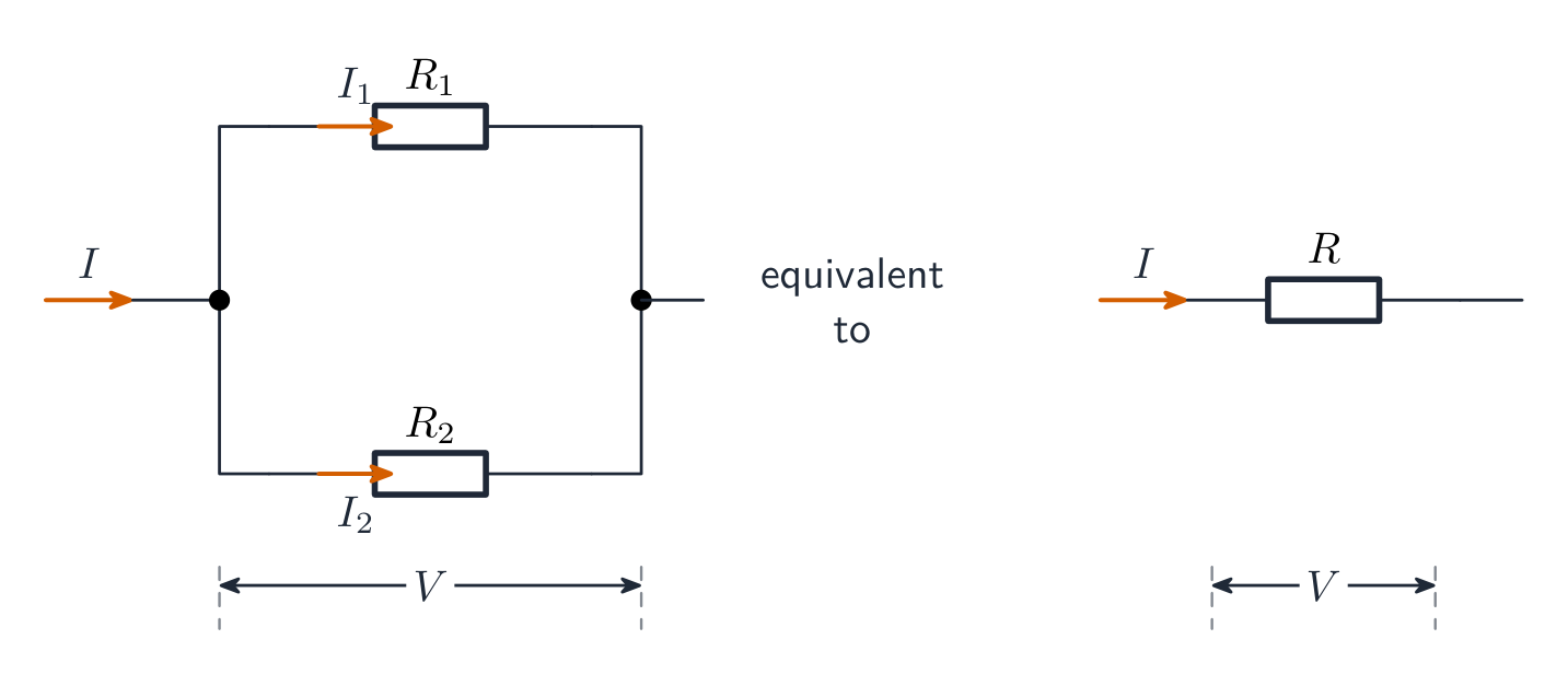
Syllabus · סיילבוס
EnglishLearning Objective 11.5.A: Describe the equivalent resistance of multiple resistors connected in a circuit.
- 11.5.A.1 Circuit elements may be connected in series and/or in parallel.
- 11.5.A.1.i A series connection is one in which any charge passing through one circuit element must proceed through all elements in that connection and has no other path available. The current in each element in series must be the same.
- 11.5.A.1.ii A parallel connection is one in which charges may pass through one of two or more paths. Across each path, the potential difference is the same.
- 11.5.A.2 A collection of resistors in a circuit may be analyzed as though it were a single resistor with an equivalent resistance $R_{\text{eq}}$.
- 11.5.A.2.i The equivalent resistance of a set of resistors in series is the sum of the individual resistances.
- Equation: $R_{\text{eq},s} = \sum_{i} R_i$
- 11.5.A.2.ii The inverse of the equivalent resistance of a set of resistors connected in parallel is equal to the sum of the inverses of the individual resistances.
- Equation: $\dfrac{1}{R_{\text{eq},p}} = \sum_{i} \dfrac{1}{R_i}$
- 11.5.A.2.iii When resistors are connected in parallel, the number of paths available to charges increases, and the equivalent resistance of the group of resistors decreases.
- 11.5.A.2.i The equivalent resistance of a set of resistors in series is the sum of the individual resistances.
Learning Objective 11.5.B: Describe a circuit with resistive wires and a battery with internal resistance.
- 11.5.B.1 Ideal batteries have negligible internal resistance. Ideal wires have negligible resistance.
- 11.5.B.1.i The resistance of wires that are good conductors may normally be neglected, because their resistance is much smaller than that of other elements of a circuit.
- 11.5.B.1.ii The resistance of wires may only be neglected if the circuit contains other elements that do have resistance.
- 11.5.B.1.iii The potential difference a battery would supply if it were ideal is the potential difference measured across the terminals when there is no current in the battery and is sometimes referred to as its $\mathrm{emf}$ ($\mathcal{E}$).
- 11.5.B.2 The internal resistance of a nonideal battery may be treated as the resistance of a resistor in series with an ideal battery and the remainder of the circuit.
- 11.5.B.3 When there is current in a nonideal battery with internal resistance $r$, the potential difference across the terminals of the battery is reduced relative to the potential difference when there is no current in the battery.
- Equation: $\Delta V_{\text{terminal}} = \mathcal{E} - Ir$
Learning Objective 11.5.C: Describe the measurement of current and potential difference in a circuit.
- 11.5.C.1 Ammeters are used to measure current at a specific point in a circuit.
- 11.5.C.1.i Ammeters must be connected in series with the element in which current is being measured.
- 11.5.C.1.ii Ideal ammeters have zero resistance so that they do not affect the current in the element that they are in series with.
- 11.5.C.2 Voltmeters are used to measure electric potential difference between two points in a circuit.
- 11.5.C.2.i Voltmeters must be connected in parallel with the element across which potential difference is being measured.
- 11.5.C.2.ii Ideal voltmeters have infinite resistance so that no charge flows through them.
- 11.5.C.3 Nonideal ammeters and voltmeters will change the properties of the circuit being measured.
Boundary statement: Unless otherwise stated, all batteries, wires, and meters are assumed to be ideal. Circuits with batteries of different potential differences connected in parallel will not be assessed.
עבריתמטרות למידה 11.5.A: לתאר התנגדות שקולה של מספר מתנגדים מחוברים במעגל.
- 11.5.A.1 רכיבי מעגל יכולים להיות מחוברים בסדרה וב/או במקביל.
- 11.5.A.1.i חיבור בסדרה הוא חיבור שבו כל מטען חולף דרך רכיב מעגלי אחד חייב לעבור דרך כל הרכיבים בחיבור זה ואין לו אופנה אחרת. עוצמת הזרם בכל רכיב בסדרה חייבת להיות זהה.
- 11.5.A.1.ii חיבור מקביל הוא חיבור שבו מטענים עשויים לעבור דרך אחד משני מסלולים או יותר. על כל מסלול, ההפרש הפוטנציאלי זהה.
- 11.5.A.2 סט של מתנגדים במעגל יכול להתנתח כאילו היהו מתנגד יחיד עם התנגדות שקולה $R_{\text{eq}}$.
- 11.5.A.2.i ההתנגדות השקולה של סט של מתנגדים בסדרה היא סכום ההתנגדויות הבודדות.
- משוואה: $R_{\text{eq},s} = \sum_{i} R_i$
- 11.5.A.2.ii ההופך של ההתנגדות השקולה של סט של מתנגדים המקוונים במקביל שווה לסכום ההופכים של ההתנגדויות הבודדות.
- משוואה: $\dfrac{1}{R_{\text{eq},p}} = \sum_{i} \dfrac{1}{R_i}$
- 11.5.A.2.iii כאשר מתנגדים מקוונים במקביל, מספר האופנות הזמינות למטענים עולה, וההתנגדות השקולה של קבוצת המתנגדים יורדת.
- 11.5.A.2.i ההתנגדות השקולה של סט של מתנגדים בסדרה היא סכום ההתנגדויות הבודדות.
מטרות למידה 11.5.B: לתאר מעגל עם חוטים התנגדותיים וסוללה עם התנגדות פנימית.
- 11.5.B.1 סוללות אידיאליות יש להן התנגדות פנימית זניחה. חוטים אידיאליים יש להם התנגדות זניחה.
- 11.5.B.1.i התנגדות חוטים שהם מוליכים טובים יכולה בדרך כלל להתעלם ממנה, מכיוון שהתנגדותם קטנה משמעותית מזו של רכיבים אחרים במעגל.
- 11.5.B.1.ii התנגדות החוטים יכולה להתעלם ממנה רק אם המעגל מכיל רכיבים אחרים שיש להם התנגדות.
- 11.5.B.1.iii הפרש הפוטנציאל שמסוללה הייתה מספקת אם הייתה אידיאלית הוא הפרש הפוטנציאל שנמדד בין הקולות כאשר אין זרם בסוללה, ומכונה לעיתים קרובות כ-$\mathrm{emf}$ ($\mathcal{E}$).
- 11.5.B.2 ההתנגדות הפנימית של סוללה שאינה אידיאלית יכולה להתנהל כהתנגדות של מתנגד בסדרה עם סוללה אידיאלית ושאר המעגל.
- 11.5.B.3 כאשר יש זרם בסוללה שאינה אידיאלית עם התנגדות פנימית $r$, הפרש הפוטנציאל בין קולות הסוללה מצומצם ביחס להפרש הפוטנציאל כאשר אין זרם בסוללה.
- משוואה: $\Delta V_{\text{terminal}} = \mathcal{E} - Ir$
מטרות למידה 11.5.C: לתאר מדידת זרם והפרש פוטנציאל במעגל.
- 11.5.C.1 אמפרמטרים משמשים למדידת זרם בנקודה ספציפית במעגל.
- 11.5.C.1.i אמפרמטרים חייבים להיות מחוברים בסדרה עם האלמנט בו נמדד הזרם.
- 11.5.C.1.ii אמפרמטרים אידיאליים הם בעלי התנגדות אפס כדי שלא ישנו את הזרם באלמנט בו הם מחוברים בסדרה.
- 11.5.C.2 וולטמטרים משמשים למדידת הפרש פוטנציאל חשמלי בין שתי נקודות במעגל.
- 11.5.C.2.i וולטמטרים חייבים להיות מחוברים במקביל לאלמנט שעליו נמדד הפרש הפוטנציאל.
- 11.5.C.2.ii וולטמטרים אידיאליים בעלי התנגדות אינסופית כך שאין זרימת מטען דרכם.
- 11.5.C.3 אמפרמטרים ווולטמטרים לא-אידיאליים יעבירו שינוי בתכונות המעגל הנמדד.
הצהרת גבול: אלא אם כן צוין אחרת, כל הסוללות, החוטים והמדדים נחשבים לאידיאליים. מעגלים המכילים סוללות עם הפרשי פוטנציאל שונים המחוברים במקביל לא יהיו נכללים בבחינה.
Source: College Board AP Course and Exam Description · מקור: תיאור הקורס והמבחן של College Board AP
Reduce resistor networks to an equivalent resistance 等效电阻: series resistances add ($R_{\text{eq}}=R_1+R_2+\cdots$), while parallel resistances add as reciprocals ($\tfrac{1}{R_{\text{eq}}}=\tfrac{1}{R_1}+\tfrac{1}{R_2}+\cdots$ – always less than the smallest branch). Collapse the network step by step to find the battery current, then expand back out to find each element's current and voltage.
Worked example. A $12\ \text{V}$ battery drives a $4.0\ \Omega$ and a $2.0\ \Omega$ resistor in series: $R_{\text{eq}}=6.0\ \Omega$, $I=2.0\ \text{A}$, the voltages split $8.0\ \text{V}$ and $4.0\ \text{V}$, and the $4.0\ \Omega$ resistor dissipates $P=I^2R=16\ \text{W}$.
Resistors in parallel combine to a smaller equivalent resistance Real batteries are not ideal. Model a battery as an ideal battery 理想电池 of emf $\varepsilon$ in series with its own internal resistance 内阻 $r$. When current flows, some emf is used up inside, so the terminal voltage 端电压 – what a voltmeter across the battery actually reads – drops:
$$\Delta V_{\text{terminal}}=\varepsilon-Ir.$$Worked example. A battery with $\varepsilon=12\ \text{V}$ and $r=0.50\ \Omega$ supplies $2.0\ \text{A}$: the terminals sit at $\Delta V=12-2.0(0.50)=11\ \text{V}$. With no current, a voltmeter reads the full $12\ \text{V}$.
Meters: an ammeter 电流表 goes in series at the point whose current you want (ideal ammeter: zero resistance); a voltmeter 电压表 goes in parallel across the element (ideal voltmeter: infinite resistance). Non-ideal meters disturb the circuit they measure – a real ammeter adds series resistance, a real voltmeter steals current.
Vocabulary · מילון מונחים Train · אימוןEnglish עברית equivalent resistance/ɪˈkwɪvələnt rɪˈzɪstəns/ התנגדות שקולה ideal battery/aɪˈdɪəl ˈbætəri/ סוללה אידיאלית internal resistance/ɪnˈtɜːnl rɪˈzɪstəns/ התנגדות פנימית terminal voltage/ˈtɜːmɪnl ˈvəʊltɪdʒ/ מתח טרמינלים ammeter/ˈæmiːtə/ ממוס voltmeter/ˈvəʊltmiːtə/ וולמטר 11.6
Kirchhoff's Loop Rule
Syllabus · סיילבוס
EnglishLearning Objective 11.6.A: Describe a circuit or elements of a circuit by applying Kirchhoff's loop rule.
- 11.6.A.1 Energy changes in simple electrical circuits may be represented in terms of charges moving through electric potential differences within circuit elements.
- Equation: $\Delta U_E = q\Delta V$
- 11.6.A.2 Kirchhoff's loop rule is a consequence of the conservation of energy.
- 11.6.A.2.i Kirchhoff's loop rule states that the sum of potential differences across all circuit elements in a single closed loop must equal zero.
- Equation: $\sum \Delta V = 0$
- 11.6.A.2.ii The values of electric potential at points in a circuit can be represented by a graph of electric potential as a function of position within a loop.
- 11.6.A.2.i Kirchhoff's loop rule states that the sum of potential differences across all circuit elements in a single closed loop must equal zero.
עבריתמטרת למידה 11.6.A: לתאר מעגל או אלמנטים במעגל באמצעות יישום חוק הלולאה של קירכהוף.
- 11.6.A.1 שינויים באנרגיה במעגלים חשמליים פשוטים יכולים להוצג באמצעות מטענים הנעים דרך הפרשי פוטנציאל חשמלי בתוך אלמנטים במעגל.
- משוואה: $\Delta U_E = q\Delta V$
- 11.6.A.2 חוק הלולאה של קירכהוף הוא תוצאה של חוק השימור של אנרגיה.
- 11.6.A.2.i חוק הלולאה של קירשוף קובע כי סכום ההפרשים הפוטנציאליים על פני כל רכיבי המעגל בלולאה סגורה אחת חייב להיות שווה לאפס.
- משוואה: $\sum \Delta V = 0$
- 11.6.A.2.ii ערכי הפוטנציאל החשמלי בנקודות במעגל יכולים להוצג באמצעות גרף של פוטנציאל חשמלי כתלות במיקום בתוך לולאה.
- 11.6.A.2.i חוק הלולאה של קירשוף קובע כי סכום ההפרשים הפוטנציאליים על פני כל רכיבי המעגל בלולאה סגורה אחת חייב להיות שווה לאפס.
Source: College Board AP Course and Exam Description · מקור: תיאור הקורס והמבחן של College Board AP
Charges moving through potential differences exchange energy ($\Delta U_E=q\Delta V$), and energy must balance around any closed path. That is Kirchhoff's loop rule 基尔霍夫回路定则:
$$\sum\Delta V=0\ \text{around any closed loop}.$$Sign discipline wins these problems: crossing a battery from $-$ to $+$ is $+\varepsilon$; crossing a resistor with the assumed current is $-IR$ (against it, $+IR$). Write one equation per independent loop.
Vocabulary · מילון מונחים Train · אימוןEnglish עברית Kirchhoff's loop rule/ˈkɜːkhɒfs luːp ruːl/ חוק הלולאה של קירשוף 11.7
Kirchhoff's Junction Rule
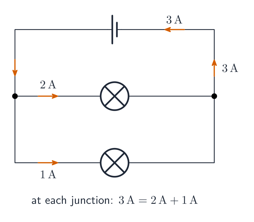
Syllabus · סיילבוס
EnglishLearning Objective 11.7.A: Describe a circuit or elements of a circuit by applying Kirchhoff's junction rule.
- 11.7.A.1 Kirchhoff's junction rule is a consequence of the conservation of electric charge.
- 11.7.A.2 Kirchhoff's junction rule states that the total amount of charge entering a junction per unit time must equal the total amount of charge exiting that junction per unit time.
- Equation: $\sum I_{\text{in}} = \sum I_{\text{out}}$
עבריתמטרת למידה 11.7.A: לתאר מעגל או אלמנטים במעגל באמצעות יישום חוק הצומת של קירכהוף.
- 11.7.A.1 חוק הצומת של קירכהוף הוא תוצאה של חוק השימור של מטען חשמלי.
- 11.7.A.2 חוק הצומת של קירכהוף קובע שהסך הכל של המטען הנכנס לצומת ביחידת זמן חייב להיות שווה לסך הכל של המטען היוצא מצומת זה ביחידת זמן.
- משוואה: $\sum I_{\text{in}} = \sum I_{\text{out}}$
Source: College Board AP Course and Exam Description · מקור: תיאור הקורס והמבחן של College Board AP
Kirchhoff's junction rule 基尔霍夫节点定则 is conservation of charge at a junction 节点:
$$\sum I_{\text{in}}=\sum I_{\text{out}}.$$Current divides at a junction: what flows in equals what flows out Together the two rules solve any multi-loop circuit: assign a current to each branch, write junction equations, then loop equations, and solve. A negative answer just means that current flows opposite to your assumed direction.
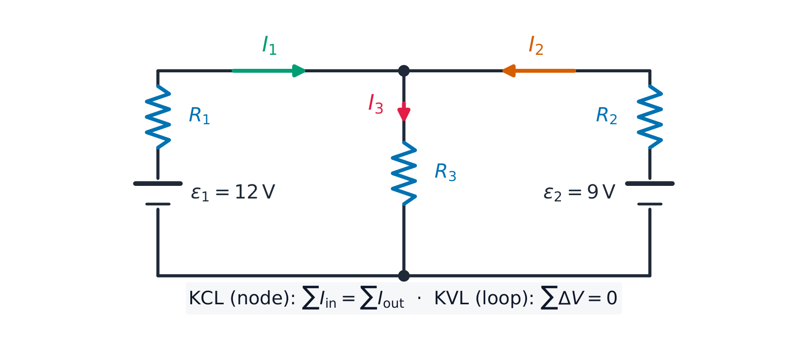
Two loop equations and one junction equation solve this two-battery circuit Worked example. In the circuit above, $\varepsilon_1=12\ \text{V}$ with $R_1=1.0\ \Omega$ on the left, $\varepsilon_2=9.0\ \text{V}$ with $R_2=1.0\ \Omega$ on the right, and a shared middle resistor $R_3=2.0\ \Omega$ carrying $I_3=I_1+I_2$ (junction rule). The two loop equations are
$$12=I_1+2(I_1+I_2)=3I_1+2I_2,\qquad 9=I_2+2(I_1+I_2)=2I_1+3I_2.$$Solving: $I_1=3.6\ \text{A}$, $I_2=0.60\ \text{A}$, so $I_3=4.2\ \text{A}$ through the middle. Check with the second loop: $2(3.6)+3(0.60)=9.0$ ✓.
Vocabulary · מילון מונחים Train · אימוןEnglish עברית Kirchhoff's junction rule/ˈkɜːkhɒfs ˈdʒʌŋkʃn ruːl/ חוק הצומת של קירשוף junction/ˈdʒʌŋkʃn/ נקודת חיבור 11.8
Resistor-Capacitor (RC) Circuits
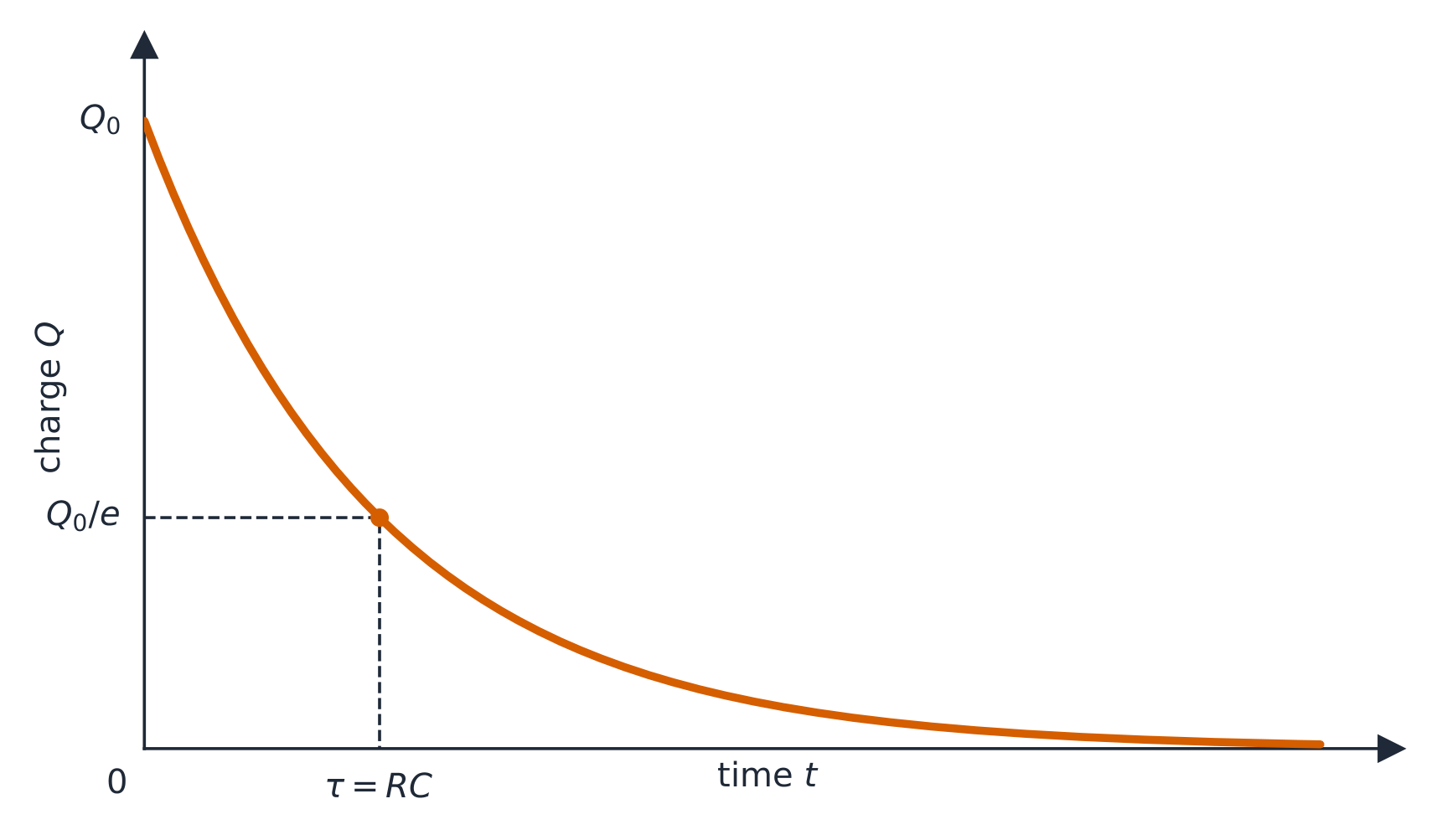
Syllabus · סיילבוס
EnglishLearning Objective 11.8.A: Describe the equivalent capacitance of multiple capacitors.
- 11.8.A.1 A collection of capacitors in a circuit may be analyzed as though it was a single capacitor with an equivalent capacitance $C_{\text{eq}}$.
- 11.8.A.1.i The inverse of the equivalent capacitance of a set of capacitors connected in series is equal to the sum of the inverses of the individual capacitances.
- Equation: $\dfrac{1}{C_{\text{eq},s}} = \sum_{i} \dfrac{1}{C_i}$
- 11.8.A.1.ii The equivalent capacitance of a set of capacitors in series is less than the capacitance of the smallest capacitor.
- 11.8.A.1.iii The equivalent capacitance of a set of capacitors in parallel is the sum of the individual capacitances.
- Equation: $C_{\text{eq},p} = \sum_{i} C_i$
- 11.8.A.1.i The inverse of the equivalent capacitance of a set of capacitors connected in series is equal to the sum of the inverses of the individual capacitances.
- 11.8.A.2 As a result of conservation of charge, each of the capacitors in series must have the same magnitude of charge on each plate.
Learning Objective 11.8.B: Describe the behavior of a circuit containing combinations of resistors and capacitors.
- 11.8.B.1 The charge on a capacitor or the current in a resistor in an RC circuit can be described by a fundamental differential equation derived from Kirchhoff's loop rule.
- Equation: $\mathcal{E} = \dfrac{dq}{dt}R + \dfrac{q}{C}$
- 11.8.B.2 The time constant ($\tau$) is a significant feature of an RC circuit.
- 11.8.B.2.i The time constant of an RC circuit is a measure of how quickly the capacitor will charge or discharge and is defined as $\tau = R_{\text{eq}}C_{\text{eq}}$.
- 11.8.B.2.ii For a charging capacitor, the time constant represents the time required for the capacitor's charge to increase from zero to approximately 63 percent of its final asymptotic value.
- 11.8.B.2.iii For a discharging capacitor, the time constant represents the time required for the capacitor's charge to decrease from fully charged to approximately 37 percent of its initial value.
- 11.8.B.3 The potential difference across a capacitor and the current in the branch of the circuit containing the capacitor each change over time as the capacitor charges and discharges, but both will reach a steady state after a long time interval.
- 11.8.B.3.i Immediately after being placed in a circuit, an uncharged capacitor acts like a wire, and charge can easily flow to or from the plates of the capacitor.
- 11.8.B.3.ii As a capacitor charges, changes to the potential difference across the capacitor affect the charge on the plates of the capacitor, the current in the circuit branch in which the capacitor is located, and the electric potential energy stored in the capacitor.
- 11.8.B.3.iii The potential difference across a capacitor, the current in the circuit branch in which the capacitor is located, and the electric potential energy stored in the capacitor all change with respect to time and asymptotically approach steady state conditions.
- 11.8.B.3.iv After a long time, a charging capacitor approaches a state of being fully charged, reaching a maximum potential difference at which there is zero current in the circuit branch in which the capacitor is located.
- 11.8.B.3.v Immediately after a charged capacitor begins discharging, the amount of charge on the capacitor and the energy stored in the capacitor begin to decrease.
- 11.8.B.3.vi As a capacitor discharges, the amount of charge on the capacitor, the potential difference across the capacitor, and the current in the circuit branch in which the capacitor is located all decrease until a steady state is reached.
- 11.8.B.3.vii After either charging or discharging for times much greater than the time constant, the capacitor and the relevant circuit branch may be modeled using steady-state conditions.
עבריתמטרת הלמידה 11.8.A: לתאר את הקיבול השווה של קבלים מרובים.
- 11.8.A.1 קבוצת קבלים במעגל ניתנת לניתוח כאילו מדובר בקבל יחיד בעל קיבול שקול $C_{\text{eq}}$.
- 11.8.A.1.i ההופך לקיבול השווה של סדרת קבלים מחוברים בסדרה שווה לסכום ההופכים של הקיבולים הבודדים.
- משוואה: $\dfrac{1}{C_{\text{eq},s}} = \sum_{i} \dfrac{1}{C_i}$
- 11.8.A.1.ii הקיבול השווה של סדרת קבלים הוא קטן מהקיבול של הקבל הקטן ביותר.
- 11.8.A.1.iii הקיבול השווה של סדרת קבלים מחוברים במקביל הוא סכום הקיבולים הבודדים.
- משוואה: $C_{\text{eq},p} = \sum_{i} C_i$
- 11.8.A.1.i ההופך לקיבול השווה של סדרת קבלים מחוברים בסדרה שווה לסכום ההופכים של הקיבולים הבודדים.
- 11.8.A.2 כתוצאה משמירת המטען, לכל אחד מהקבלים בסדרה חייב להיות אותו גודל של מטען על כל פלטה.
מטרת הלמידה 11.8.B: לתאר את התנהגות מעגל המכיל שילובים של נגדיויות וקבלים.
- 11.8.B.1 המטען על קבל או הזרם ברזיסטור במעגל RC ניתן לתיאור באמצעות משוואה דיפרנציאלית בסיסית הנגזרת מחוק הלולאה של קירשוף.
- משוואה: $\mathcal{E} = \dfrac{dq}{dt}R + \dfrac{q}{C}$
- 11.8.B.2 הקבוע הזמני ($\tau$) הוא מאפיין משמעותי במעגל RC.
- 11.8.B.2.i הקבוע הזמני של מעגל RC הוא מדד לכמה מהר הקבל יטעון או יפרק, ומוגדר כ$\tau = R_{\text{eq}}C_{\text{eq}}$.
- 11.8.B.2.ii עבור קבל בטעינה, הקבוע הזמני מייצג את הזמן הדרוש כדי שהמטען על הקבל יעלה מאפס לכ-63% מערכו האסימפטוטי הסופי.
- 11.8.B.2.iii עבור קבל בפריקה, הקבוע הזמני מייצג את הזמן הדרוש כדי שהמטען על הקבל ירד ממצב טעון לחלוטין לכ-37% מערכו ההתחלתי.
- 11.8.B.3 ההפרש הפוטנציאלי על פני קבל והזרם בענף המעגל המכיל את הקבל משתנים עם הזמן כאשר הקבל נטען ומתפרק, אך שניהם יגיעו למצב יציב לאחר מרווח זמן ארוך.
- 11.8.B.3.i מיד לאחר הוצבתו במעגל, קבל לא טעון מתנהג כמו חוט, ומטען יכול לזרום בקלות אל או מן הפלטות של הקבל.
- 11.8.B.3.ii כשהקבל נטען, שינויים בהפרש הפוטנציאלי על פני הקבל משפיעים על המטען על פלטותיו, על הזרם בענף המעגל בו הוא ממוקם ועל אנרגיה פוטנציאלית חשמלית שמאחסנת בקבל.
- 11.8.B.3.iii ההפרש הפוטנציאלי על פני הקבל, הזרם בענף המעגל בו הוא ממוקם ואנרגיה פוטנציאלית חשמלית שמאחסנת בקבל כולם משתנים ביחס לזמן וגוברים אסימפטוטית לעבר תנאי מצב יציב.
- 11.8.B.3.iv לאחר זמן ארוך, קבל בטעינה מתקרב למצב טעון לחלוטין, ומגיע להפרש פוטנציאל מקסימלי שבו אין זרם בענף המעגל בו הקבל ממוקם.
- 11.8.B.3.v מיד לאחר שהקבל הטעון מתחיל לפרק, כמות המטען על הקבל והאנרגיה המאחסנת בו מתחילות לרדת.
- 11.8.B.3.vi כשהקבל מתפרק, כמות המטען עליו, ההפרש הפוטנציאלי על פניו והזרם בענף המעגל בו הוא ממוקם כולם יורדים עד שהתנאים היציבים יושגו.
- 11.8.B.3.vii לאחר טעינה או פריקה במשך זמנים הארוכים משמעותית מהקבוע הזמני, ניתן לדגמן את הקבל ואת ענף המעגל הרלוונטי באמצעות תנאי מצב יציב.
Source: College Board AP Course and Exam Description · מקור: תיאור הקורס והמבחן של College Board AP
Discharging a capacitor: τ = RC Charging a capacitor (RC) Capacitor networks reduce like resistors but with the rules swapped: parallel capacitances add ($C_{\text{eq}}=C_1+C_2$), series add as reciprocals – and capacitors in series must carry the same charge on each plate, by conservation of charge. Use the equivalent capacitance 等效电容 to analyse the network, then expand back.
In an RC circuit RC电路, Kirchhoff's loop rule gives the differential equation
$$\varepsilon=R\frac{dq}{dt}+\frac{q}{C},$$whose solutions are exponentials with time constant 时间常数 $\tau=RC$:
$$q(t)=Q\big(1-e^{-t/RC}\big)\ \text{(charging)},\qquad q(t)=Q\,e^{-t/RC}\ \text{(discharging)},\qquad i(t)=\frac{\varepsilon}{R}e^{-t/RC}.$$The current is largest at the first instant and decays – it never "waits" for the capacitor. Learn the two limits: at $t=0$ an uncharged capacitor acts like a plain wire (maximum current); after a long time it is fully charged, no current flows in its branch, and it acts like a break. In any steady state 稳态, cover the capacitor branch with your finger, solve the resistor circuit, then read the capacitor's voltage from the element it sits across.
The charge on a capacitor decays exponentially as it discharges Worked example. With $R=5.0\ \text{k}\Omega$, $C=200\ \mu\text{F}$, and a $10\ \text{V}$ battery: $\tau=RC=1.0\ \text{s}$; initial current $\dfrac{\varepsilon}{R}=2.0\ \text{mA}$; after one time constant the charge is $q=CV(1-e^{-1})\approx1.3\times10^{-3}\ \text{C}$, about $63\%$ of full charge, and the current has fallen to $37\%$ of its initial value.
A real circuit on a breadboard: a resistor and capacitor together set how fast the voltage rises and falls Vocabulary · מילון מונחים Train · אימוןEnglish עברית equivalent capacitance/ɪˈkwɪvələnt kəˈpæsɪtəns/ קיבולת שקולה RC circuit/ˌɑː ˈsiː ˈsɜːkɪt/ מעגל RC time constant/taɪm ˈkɒnstənt/ קבוע זמן steady state/ˈstedi steɪt/ מצב יציב 11.8
Exam tips
- Relate current to charge flow $I=\tfrac{dQ}{dt}$ and use $J=\sigma E$, $R=\tfrac{\rho L}{A}$ for resistance.
- Apply Kirchhoff's laws (junction: charge; loop: energy) with consistent sign conventions.
- Analyse RC circuits with calculus: charging/discharging give exponentials with time constant $\tau=RC$.
- Combine resistors (series add, parallel reciprocal) and track power $P=IV=I^2R$.
- At $t=0$ a capacitor acts like a wire; after a long time ($t\to\infty$) it acts like an open branch.
- 11.1.A.1 Current is the rate at which charge passes through a cross-sectional area of a wire.
-
12
Magnetic Fields and Electromagnetism · שדות מגנטיים וחשמל-מגנטיות
Watch lesson · צפה בשיעור12.1
Magnetic Fields · שדות מגנטיים
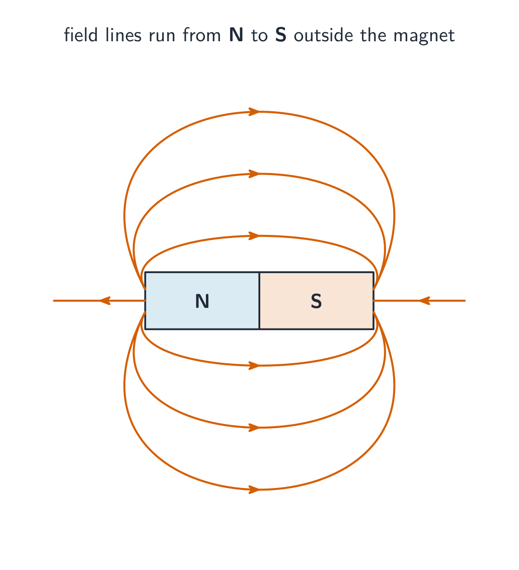
Syllabus · סיילבוס
EnglishLearning Objective 12.1.A: Describe the properties of a magnetic field.
- 12.1.A.1 A magnetic field is a vector field that can be used to determine the magnetic force exerted on moving electric charges, electric currents, or magnetic materials.
- 12.1.A.1.i Magnetic fields can be produced by magnetic dipoles or combinations of dipoles, but never by monopoles.
- 12.1.A.1.ii Magnetic dipoles have north and south polarity.
- 12.1.A.2 A magnetic field is a vector quantity and can be represented using vector field maps.
- 12.1.A.3 Magnetic field lines must form closed loops, as described by Gauss's law for magnetism.
- 12.1.A.3.i Maxwell's equations are the collection of equations that fully describe electromagnetism. Gauss's law for magnetism is Maxwell's second equation.
- Equation: $\oint \vec{B} \cdot d\vec{A} = 0$
- 12.1.A.3.ii Magnetic fields in a bar magnet form closed loops, with the external magnetic field pointing away from one end (defined as the north pole) and returning to the other end (defined as the south pole).
- 12.1.A.3.i Maxwell's equations are the collection of equations that fully describe electromagnetism. Gauss's law for magnetism is Maxwell's second equation.
Learning Objective 12.1.B: Describe the magnetic behavior of a material as a result of the configuration of magnetic dipoles in the material.
- 12.1.B.1 Magnetic dipoles result from the circular or rotational motion of electric charges. In magnetic materials, this can be the motion of electrons.
- 12.1.B.1.i Permanent magnetism and induced magnetism are system properties that both result from the alignment of magnetic dipoles within a system.
- 12.1.B.1.ii No magnetic north pole is ever found in isolation from a south pole. For example, if a bar magnet is broken in half, both halves are magnetic dipoles.
- 12.1.B.1.iii Magnetic poles of the same polarity will repel; magnetic poles of opposite polarity will attract.
- 12.1.B.1.iv The magnitude of the magnetic field from a magnetic dipole decreases with increasing distance from the dipole.
- 12.1.B.2 A magnetic dipole, such as a magnetic compass, placed in a magnetic field will tend to align with the magnetic field.
- 12.1.B.3 A material's composition influences its magnetic behavior in the presence of an external magnetic field.
- 12.1.B.3.i Ferromagnetic materials such as iron, nickel, and cobalt can be permanently magnetized by an external field that causes the alignment of magnetic domains or atomic magnetic dipoles.
- 12.1.B.3.ii Paramagnetic materials such as aluminum, titanium, and magnesium interact weakly with an external magnetic field, in that the magnetic dipoles of the material do not remain aligned after the external field is removed.
- 12.1.B.3.iii All materials have the property of diamagnetism, in that their electronic structure creates a usually weak alignment of the dipole moments of the material opposite the external magnetic field.
- 12.1.B.4 Earth's magnetic field may be approximated as a magnetic dipole.
Learning Objective 12.1.C: Describe the magnetic permeability of a material.
- 12.1.C.1 Magnetic permeability is a measurement of the amount of magnetization in a material in response to an external magnetic field.
- 12.1.C.2 Free space has a constant value of magnetic permeability, known as the vacuum permeability $\mu_0$, that appears in equations representing physical relationships.
- 12.1.C.3 The permeability of matter has values different from that of free space and arises from the matter's composition and arrangement. It is not a constant for a material and varies based on many factors, including temperature, orientation, and strength of the external field.
עבריתמטרות למידה 12.1.A: תאר את מאפייני השדה המגנטי.
- 12.1.A.1 שדה מגנטי הוא שדה וקטורי שיכול לשמש לקביעת הכוח המגנטי הפועל על מטענים חשמליים נעים, זרמים חשמליים או חומרים מגנטיים.
- 12.1.A.1.i שדות מגנטיים יכולים להיות מופקים ממגנטים דו-קוטביים (דיפולים) או משילובים של דיפולים, אך לעולם לא ממגנטים חד-קוטביים (מונופולים).
- 12.1.A.1.ii למגנטים דו-קוטביים יש קוטביות צפונית ודרומית.
- 12.1.A.2 שדה מגנטי הוא גודל וקטורי ואפשר להציג אותו באמצעות מפות שדה וקטוריות.
- 12.1.A.3 קווי השדה המגנטי חייבים ליצור לולאות סגורות, כפי שמתואר בחוק גאוס למגנטיות.
- 12.1.A.3.i משוואות מקסוול הן קבוצת המשוואות המתארת במלואה את האלקטרומגנטיות. חוק גאוס למגנטיות הוא המשוואה השנייה של מקסוול.
- משוואה: $\oint \vec{B} \cdot d\vec{A} = 0$
- 12.1.A.3.ii שדות מגנטיים בסוגר מבר יוצרים לולאות סגורות, כאשר השדה המגנטי החיצוני מכוון הרחק מאחד הקצה (שהוגדר כקוטב צפוני) וחוזר לקצה השני (שהוגדר כקוטב דרומי).
- 12.1.A.3.i משוואות מקסוול הן קבוצת המשוואות המתארת במלואה את האלקטרומגנטיות. חוק גאוס למגנטיות הוא המשוואה השנייה של מקסוול.
מטרות למידה 12.1.B: תאר את ההתנהגות המגנטית של חומר כתוצאה מהקונפיגורציה של הדיפולים המגנטיים בתוכו.
- 12.1.B.1 דיפולים מגנטיים נובעים מתנועה מעגלית או סיבובית של מטענים חשמליים. בחומרים מגנטיים, זה עשוי להיות תנועת אלקטרונים.
- 12.1.B.1.i מגנטיות קבועה ומגנטיות מושרדת הן מאפייני מערכת הנובעים משנייהם מהסדרת הדיפולים המגנטיים בתוך המערכת.
- 12.1.B.1.ii לעולם לא נמצא קוטב צפוני בודד ללא קוטב דרומי. לדוגמה, אם מקלט בר נשבר לחצי, כל מחצית היא דיפול מגנטי.
- 12.1.B.1.iii קוטבים מגנטיים בעלי אותה קוטביות ידחו זה את זה; קוטבים מגנטיים בעלי קוטביות הפוכה יתארו זה עם זה.
- 12.1.B.1.iv הגודל של השדה המגנטי מדיפול מגנטי יור随着 העלייה במרחק מהדיפול.
- 12.1.B.2 דיפול מגנטי, כמו מצפן מגנטי, הממוקם בשדה מגנטי י tende להתארגן בהתאם לשדה המגנטי.
- 12.1.B.3 הרכב החומר משפיע על התנהגותו המגנטית בנוכחות שדה מגנטי חיצוני.
- 12.1.B.3.i חומרים פרומגנטיים כמו ברזל, ניקל וקובלט יכולים להיות מוגנטיים באופן קבוע על ידי שדה חיצוני הגורם לסדרת הדומיינים המגנטיים או הדיפולים האטומיים המגנטיים.
- 12.1.B.3.ii חומרים פאראמגנטיים כמו אלומיניום, טיטניום ומגנזיום מתאימים בצורה חלשה לשדה מגנטי חיצוני, שכן הדיפולים המגנטיים של החומר אינם נשארים מסודרים לאחר הסרת השדה החיצוני.
- 12.1.B.3.iii לכל החומרים יש את התכונה של דיאמגנטיות, שבה המבנה האלקטרוני שלהם יוצר סדרת דיפולים בדרך כלל חלשה בכיוון הפוך לשדה המגנטי החיצוני.
- 12.1.B.4 השדה המגנטי של כדור הארץ ניתן לקירוב כדיפול מגנטי.
מטרה לימודית 12.1.C: לתאר את הנפגעות המגנטית של חומר.
- 12.1.C.1 נפגעות מגנטית היא מידה לכמות ההתמגנות בחומר כתגובה לשדה מגנטי חיצוני.
- 12.1.C.2 לחלל הפנוי יש ערך קבוע של נפגעות מגנטית, המכונה נפגעות וקום $\mu_0$, הופיע במשוואות המייצגות קשרים פיזיקליים.
- 12.1.C.3 לנפגעות החומר יש ערכים שונים מזה של החלל הפנוי והיא נובעת מההרכב והסידור של החומר. היא אינה קבועה עבור חומר מסוים ומשתנה בהתאם לגורמים רבים, כולל טמפרטורה, כיוון וחוזק השדה החיצוני.
Source: College Board AP Course and Exam Description · מקור: תיאור הקורס והמבחן של College Board AP
EnglishA magnetic field 磁场 $\vec{B}$ is a vector field 矢量场 that surrounds magnets, moving charges, and currents; it determines the magnetic force on any moving charge placed in it. Magnetic field lines 磁感线 must form closed loops: they leave the north pole, return to the south pole, and continue through the magnet. Denser lines mean a stronger field.
Closed loops are the content of Gauss's law for magnetism, the second of Maxwell's equations 麦克斯韦方程组:
$$\oint \vec{B}\cdot d\vec{A}=0.$$The net magnetic flux through any closed surface is zero – as many field lines leave as enter. That is exactly the statement that isolated magnetic monopoles 磁单极子 do not exist. Every source of magnetism is a magnetic dipole 磁偶极子 (a north–south pair), made by circulating charge – in materials, the motion of electrons. Break a bar magnet in half and you get two smaller dipoles, never a lone pole. Like poles repel, opposite poles attract, and a free dipole – a compass 指南针 – rotates to line up with the local field. Earth's own field is approximately a dipole, which is why a compass works. Dipole fields weaken with distance.
How a material responds to an external field depends on how its internal dipoles behave:
- Ferromagnetic 铁磁性 (iron, nickel, cobalt): an external field aligns whole magnetic domains 磁畴, and the alignment survives after the field is removed – a permanent magnet.
- Paramagnetic 顺磁性 (aluminum, titanium): dipoles align weakly with the field but relax when it is removed.
- Diamagnetic 抗磁性 (all materials): the electronic structure produces a usually weak alignment opposite to the field.
The strength of a material's response is its magnetic permeability 磁导率. Free space has the constant value $\mu_0$ (the vacuum permeability); the permeability of matter differs from $\mu_0$ and is not even constant – it varies with temperature, orientation, and field strength.
עבריתשדה מגנטי $\vec{B}$ הוא שדה וקטורי המקיף מגנטים, מטענים זזים וזרמים; הוא קובע את הכוח המגנטי על כל מטען זז המופקם בו. קווי שדה מגנטי חייבים ליצור לולאות סגורות: הם יוצאים מקוטב הצפון, חוזרים לקוטב הדרום, וממשיכים דרך המגנט. קווים צפופים יותר מעידים על שדה חזק יותר.
קווי שדה עוברים מ-N ל-S מחוץ למגנט מוט לולאות סגורות הן תוכן חוק גאוס למגנטיות, השני במשוואות מקסוול:
$$\oint \vec{B}\cdot d\vec{A}=0.$$השטף המגנטי הכולל דרך כל פני שטח סגורים הוא אפילו – אותו מספר קווי שדה יוצא כמו שנכנס. זה בדיוק הביע לכך שאין מונופולים מגנטיים מבודדים. כל מקור של מגנטיות הוא דו-קוטב מגנטי (זוג צפון-דרום), שנוצר על ידי מטען מסתובב – בחומרים, זה תנועת אלקטרונים. שביתו מגנט מוט לשניים ותקבלו שני דו-קוטבים קטנים יותר, לעולם לא קוטב בודד. קוטבים זהים דוחים, קוטבים מנוגדים מושכים, ודו-קוטב חופשי – מצפן – מסתובב כדי להסתדר עם השדה המקומי. השדה של כדור הארץ הוא בקירוב דו-קוטב, ולכן מצפן עובד. שדות דו-קוטבים חולשים עם המרחק.
התגובה של חומר לשדה חיצוני תלויה בהתנהגות המונופולים הפנימיים שלו:
- פרומגנטי (ברזל, ניקל, קובלט): שדה חיצוני מיישר את כל הדומיינים המגנטיים, והיישור נשמר לאחר הסרת השדה – מגנט קבוע.
- פאראמגנטי (אלומיניום, טיטניום): המונופולים מתיישבים בחולשה עם השדה אך מתרופפים כאשר הוא מוסר.
- דיאמגנטי (כל החומרים): המבנה האלקטרוני יוצר לרוב יישור חלש נגד כיוון השדה.
עוצמת התגובה של החומר היא החדירות המגנטית. לחלל ריק יש ערך קבוע $\mu_0$ (חדירות הוואקום); חדירות החומר שונה מ-$\mu_0$ ואף אינה קבועה – היא משתנה לפי טמפרטורה, כיוון ועוצמת השדה.

אורורה: חלקיקים טעונים מהשמש מכוונים על ידי השדה המגנטי של כדור הארץ לכיוון הקוטבים Explore · חקורSee a magnet's field lines · ראה קווי שדה מגנטי
Magnetic field lines run from north to south outside a magnet; where they crowd together the field is strongest. · קווי שדה מגנטי עוברים מצפון לדרום מחוץ למגנט; כשהם צפופים יחד השדה חזק ביותר.
12.2
Magnetism and Moving Charges · מגנטיות ומטענים זזים
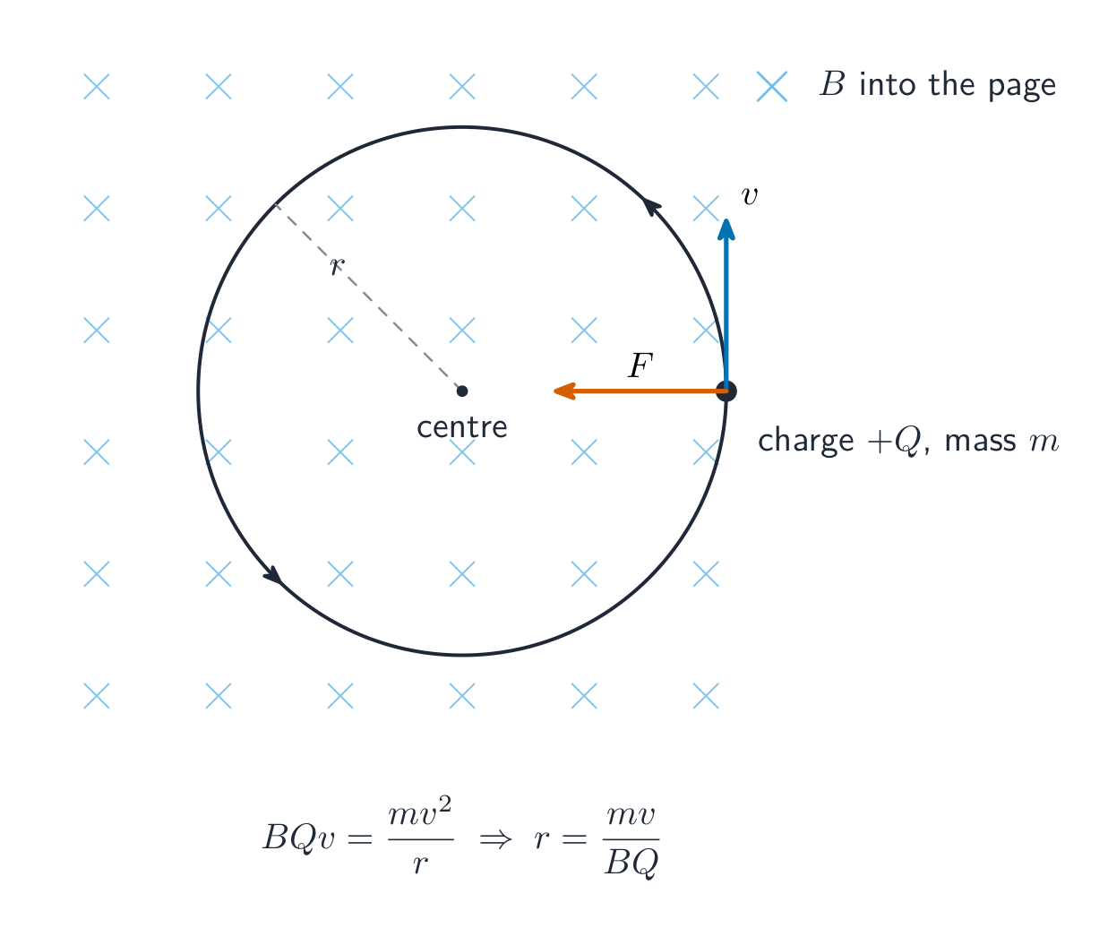
Syllabus · סיילבוס
EnglishLearning Objective 12.2.A: Describe the magnetic field produced by moving charged objects.
- 12.2.A.1 A single moving charged object produces a magnetic field.
- 12.2.A.1.i The magnetic field at a particular point produced by a moving charged object depends on the object's velocity and the distance between the point and the object.
- 12.2.A.1.ii At a point in space, the direction of the magnetic field produced by a moving charged object is perpendicular to both the velocity of the object and the position vector from the object to that point in space and can be determined using the right-hand rule.
- 12.2.A.1.iii The magnitude of the magnetic field is a maximum when the velocity vector and the position vector from the object to that point in space are perpendicular.
Learning Objective 12.2.B: Describe the force exerted on moving charged objects by a magnetic field.
- 12.2.B.1 A magnetic field will exert a force on a charged object moving within that field, with magnitude and direction that depend on the cross-product of the charge's velocity and the magnetic field.
- Equation: $\vec{F}_B = q\left(\vec{v} \times \vec{B}\right)$
- 12.2.B.2 In a region containing both a magnetic field and an electric field, a moving charged object will experience independent forces from each field.
- 12.2.B.3 The Hall effect describes the potential difference created in a conductor by an external magnetic field that has a component perpendicular to the direction of charges moving in the conductor.
עבריתמטרה לימודית 12.2.A: לתאר את השדה המגנטי הנוצר על ידי אובייקטים טעונים הזזים.
- 12.2.A.1 אובייקט טעון זז יחיד מייצר שדה מגנטי.
- 12.2.A.1.i השדה המגנטי בנקודה ספציפית הנוצר על ידי אובייקט טעון זז תלוי במהירות האובייקט ובמרחק בין הנקודה לבין האובייקט.
- 12.2.A.1.ii בנקודה במרחב, הכיוון של השדה המגנטי הנוצר על ידי אובייקט טעון זז מאונך גם למהירות האובייקט וגם לווקטור המיקום מהאובייקט לנקודה זו במרחב,并可确定使用右手定则。 (Note: The original text had a mix of English and Chinese here; translating the full concept: ) ניתן לקבוע זאת באמצעות כלל היד הימנית.
- 12.2.A.1.iii הגודל של השדה המגנטי הוא מקסימלי כאשר וקטור המהירות ווקטור המיקום מהאובייקט לנקודה זו במרחב מאונכים זה לזה.
מטרה לימודית 12.2.B: לתאר את הכוח הפועל על אובייקטים טעונים זזים על ידי שדה מגנטי.
- 12.2.B.1 שדה מגנטי יפעיל כוח על אובייקט טעון הנע בתוך השדה, עם גודל וכיוון התלויים בכפל וקטורי של מהירות הטעינה והשדה המגנטי.
- משוואה: $\vec{F}_B = q\left(\vec{v} \times \vec{B}\right)$
- 12.2.B.2 באזור המכיל גם שדה מגנטי וגם שדה חשמלי, אובייקט טעון הנע יחווה כוחות עצמאיים מכל שדה.
- 12.2.B.3 אפקט הול מתאר הפרש פוטנציאל הנוצר במוליך על ידי שדה מגנטי חיצוני בעל רכיב אנכי לכיוון תנועת הטעונים במוליך.
Source: College Board AP Course and Exam Description · מקור: תיאור הקורס והמבחן של College Board AP
EnglishA moving charge in a magnetic field A moving charge does two things: it creates a magnetic field, and it feels a force in an external one. The field it creates at a point is perpendicular 垂直 to both its velocity and the position vector from charge to point (right-hand rule again), and is largest where those two are perpendicular – zero directly ahead of or behind the motion.
The force on a charge moving in a field $\vec{B}$ is the cross product
$$\vec{F}_B=q\,\vec{v}\times\vec{B},\qquad F=qvB\sin\theta,$$perpendicular to both $\vec{v}$ and $\vec{B}$ – point the fingers of your right hand along $\vec{v}$, curl toward $\vec{B}$, and the thumb gives the force on a positive charge (reverse it for negative). Because $\vec{F}_B\perp\vec{v}$, the magnetic force does no work on the charge: it changes direction, never speed.
A charge moving perpendicular to a uniform field therefore travels in a circle, the magnetic force supplying the centripetal force 向心力:
$$qvB=\frac{mv^2}{r}\quad\Rightarrow\quad r=\frac{mv}{qB},\qquad T=\frac{2\pi m}{qB}.$$Notice the period $T$ does not depend on the speed – faster particles ride larger circles in the same time.
Worked example. A proton ($q=1.6\times10^{-19}\ \text{C}$, $m=1.67\times10^{-27}\ \text{kg}$) enters a $0.50\ \text{T}$ field at $2.0\times10^{5}\ \text{m/s}$, perpendicular to it. The magnetic force $F=qvB=1.6\times10^{-14}\ \text{N}$ bends it into a circle of radius $r=\dfrac{mv}{qB}=\dfrac{1.67\times10^{-27}(2.0\times10^{5})}{1.6\times10^{-19}(0.50)}=4.2\times10^{-3}\ \text{m}$.
In a region with both an electric and a magnetic field, the two forces act independently and add as vectors. Balancing them makes a velocity selector 速度选择器: with $\vec{E}$ and $\vec{B}$ crossed, only charges with $qE=qvB$, i.e. $v=E/B$, pass straight through. The Hall effect 霍尔效应 is the same physics inside a conductor: a field with a component perpendicular to the current pushes the moving carriers sideways, charge builds up on one face, and a measurable potential difference appears across the conductor – its sign reveals whether the carriers are positive or negative.
עבריתמטען נע בשדה מגנטי מטען הנע לבצע שתי פעולות: הוא יוצר שדה מגנטי, וזה חש בכוח בשדה חיצוני. השדה שהוא יוצר בנקודה נתונה הוא ניצב לגבי גם מהירותו וגם וקטור המיקום ממטען לנקודה (שוב כלל היד הימנית), והוא מקסימלי שם ששניהם ניצבים זה לזה – אפס בדיוק קדימה או אחורה לתנועה.
הכוח על מטען הנע בשדה $\vec{B}$ הוא מכפלה וקטורית
$$\vec{F}_B=q\,\vec{v}\times\vec{B},\qquad F=qvB\sin\theta,$$ניצבה לשני $\vec{v}$ ול-$\vec{B}$ – נקודו אצבעות היד הימנית לאורך $\vec{v}$, כיפפו לעבר $\vec{B}$, והאגודל מצביע על הכוח על מטען חיובי (הפכו עבור מטען שלילי). מכיוון ש-$\vec{F}_B\perp\vec{v}$, הכוח המגנטי אינו מבצע עבודה על המטען: הוא משנה כיוון, לעולם אינו משנה מהירות.
מטען הנע בניצב לשדה אחיד לכן נע במעגל, כאשר הכוח המגנטי מספק את הכוח המרכזי:
$$qvB=\frac{mv^2}{r}\quad\Rightarrow\quad r=\frac{mv}{qB},\qquad T=\frac{2\pi m}{qB}.$$שימו לב שהתקופה $T$ אינה תלויה במהירות – חלקיקים מהירים יותר רוכבים על מעגלים גדולים יותר באותו זמן.
חלקיק טעון הנע אופקית לשדה מגנטי עוקף מסלול מעגלי דוגמה פתורה. פרוטון ($q=1.6\times10^{-19}\ \text{C}$, $m=1.67\times10^{-27}\ \text{kg}$) נכנס לשדה $0.50\ \text{T}$ במהירות $2.0\times10^{5}\ \text{m/s}$, בניצב אליו. הכוח המגנטי $F=qvB=1.6\times10^{-14}\ \text{N}$ מכופף אותו למעגל ברדיוס $r=\dfrac{mv}{qB}=\dfrac{1.67\times10^{-27}(2.0\times10^{5})}{1.6\times10^{-19}(0.50)}=4.2\times10^{-3}\ \text{m}$.
באזור בו ישנם גם שדה חשמלי וגם שדה מגנטי, שני הכוחות פועלים באופן עצמאי ומת加ים כוקטורים. איזון ביניהם יוצר מסנן מהירות: עם $\vec{E}$ ו-$\vec{B}$ ניצבים זה לזה, רק מטענים בעלי $qE=qvB$, כלומר $v=E/B$, עוברים ישר דרכו. אפקט הול הוא אותה פיזיקה בתוך מוליך: שדה עם רכיב ניצב לזרם דוחף את נושאי המטען הנעים צדדים, מטען מצטבר על צד אחד, ומתקבל הפרש פוטנציאל מדיד בין צדדים – סימונו חושף האם נושאי המטען הם חיוביים או שליליים.
Explore · חקורForce on a moving charge · כוח על מטען הנע
A charge moving through a magnetic field feels a force $F=qvB$ at right angles to both its velocity and the field — the basis of the motor effect. Reverse either and the force flips. · מטען הנע דרך שדה מגנטי מרגיש כוח $F=qvB$ המאונך גם לכיוון מהירותו וגם לשדה — בסיס אפקט המנוע. הפיכת אחד מהם הופכת את הכוח.
12.3
Magnetic Fields of Current-Carrying Wires · שדות מגנטיים של חוטים המוליכים זרם
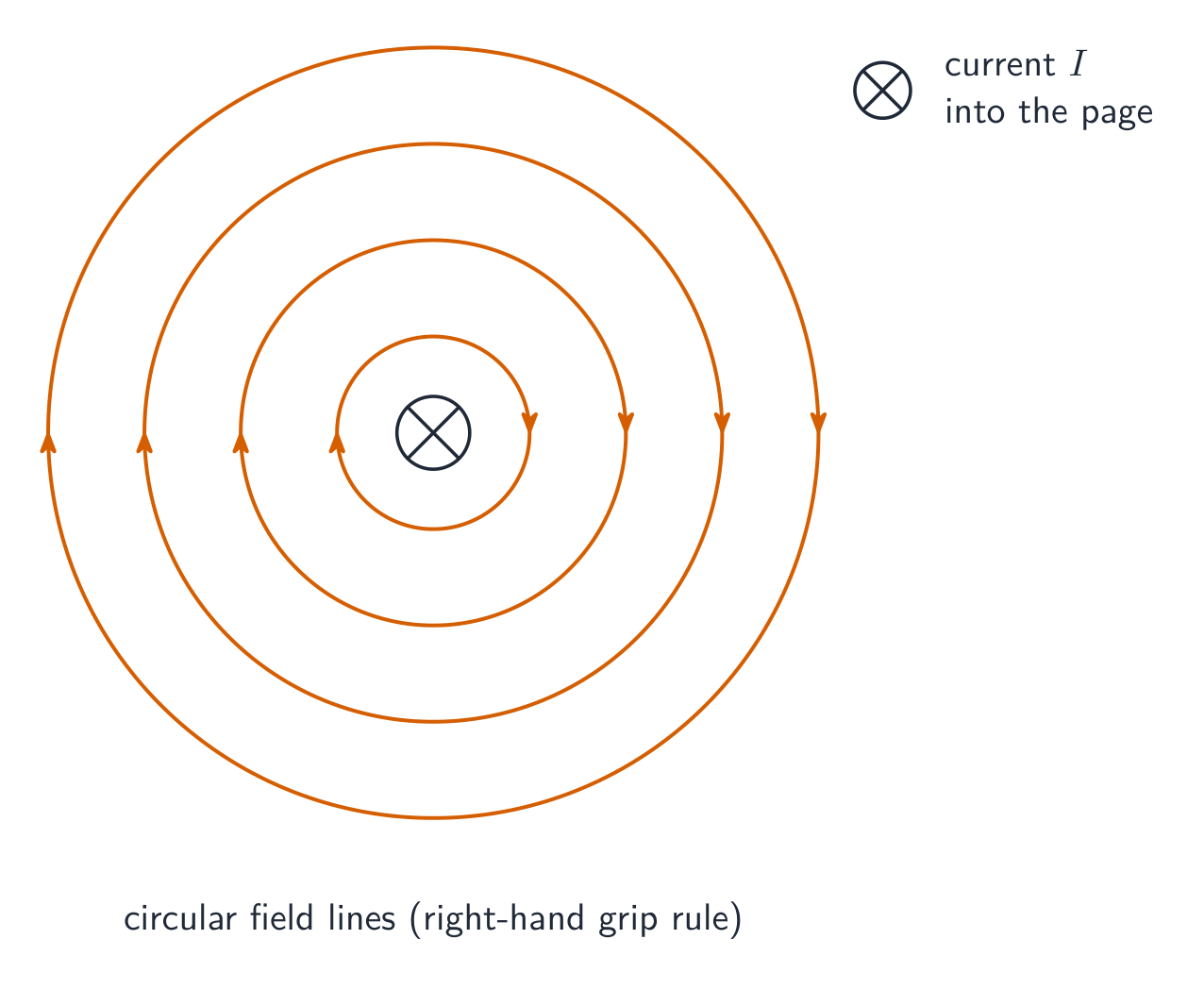
Syllabus · סיילבוס
EnglishLearning Objective 12.3.A: Describe the magnetic field produced by a current-carrying wire.
- 12.3.A.1 The Biot-Savart law defines the magnitude and direction of a magnetic field created by an electrical current.
- Equation: $d\vec{B} = \dfrac{\mu_0}{4\pi} \dfrac{I(d\vec{\ell} \times \hat{r})}{r^2}$
- 12.3.A.2 The magnetic field vectors around a small segment of a current-carrying wire are tangent to concentric circles centered on that wire. The field has no component toward, away from, or parallel to the segment of the current-carrying wire.
- 12.3.A.3 The Biot-Savart law can be used to derive the magnitudes and directions of magnetic fields around segments of current-carrying wires, for example at the center of a circular loop of wire.
- Equation: $B_{\text{center of loop}} = \dfrac{\mu_0 I}{2R}$
Learning Objective 12.3.B: Describe the force exerted on current-carrying wires by a magnetic field.
- 12.3.B.1 A magnetic field will exert a force on a current-carrying wire.
- Equation: $\vec{F}_B = \int I\left(d\vec{\ell} \times \vec{B}\right)$
Boundary statement: AP Physics C: Electricity & Magnetism only expects students to perform quantitative analysis of certain cases of current-carrying conductors using the Biot-Savart law, such as at a location along the perpendicular bisector of a straight conductor, at a location along the central axis of a circular loop, or at the center of a segment of a circular loop.
עבריתמטרה לימודית 12.3.A: לתאר את השדה המגנטי הנוצר על ידי חוט המעביר זרם.
- 12.3.A.1 חוק ביאו-סבאר מגדיר את הגודל והכיוון של שדה מגנטי הנוצר על ידי זרם חשמלי.
- משוואה: $d\vec{B} = \dfrac{\mu_0}{4\pi} \dfrac{I(d\vec{\ell} \times \hat{r})}{r^2}$
- 12.3.A.2 וקטורי השדה המגנטי סביב קטע קטן של חוט נושא זרם הם מגעים לעיגולים ממוקדים הממוקמים על אותו חוט. לשדה אין רכיב כלפי, מרחק או מקביל לקטע החוט נושא הזרם.
- 12.3.A.3 ניתן להשתמש בחוק ביאו-סבאר כדי לגזור את הגדלים והכיוונים של שדות מגנטיים סביב קטעים של חוטים נושאי זרם, לדוגמה במרכז לולאת חוט מעגלית.
- משוואה: $B_{\text{center of loop}} = \dfrac{\mu_0 I}{2R}$
מטרת הלמידה 12.3.B: לתאר את הכוח הפועל על חוטים נושאי זרם על ידי שדה מגנטי.
- 12.3.B.1 שדה מגנטי יפעיל כוח על חוט נושא זרם.
- משוואה: $\vec{F}_B = \int I\left(d\vec{\ell} \times \vec{B}\right)$
הצהרת גבול: AP Physics C: חשמל ומגנטיות מצפה רק מבחינת הסטודנטים לבצע ניתוח כמותי של מקרים מסוימים של מוליכים נושאי זרם באמצעות חוק ביאו-סבאר, כמו במיקום לאורך האנך האמצעי של מוליך ישר, במיקום לאורך הציר המרכזי של לולאה מעגלית, או במרכז קטע של לולאה מעגלית.
Source: College Board AP Course and Exam Description · מקור: תיאור הקורס והמבחן של College Board AP
EnglishThe magnetic field around a current A current is a stream of moving charges, so it creates a magnetic field. The Biot–Savart law 毕奥-萨伐尔定律 adds up the field of each current element:
$$d\vec{B}=\frac{\mu_0}{4\pi}\frac{I\,d\vec{l}\times\hat{r}}{r^2}.$$Around any straight segment the field vectors are tangent 相切 to concentric circles 同心圆 centred on the wire – no component toward, away from, or along the wire. Curl your right hand around the wire with the thumb along the current: your fingers give the field direction.
The Biot–Savart integrals AP expects: a long straight wire ($B=\dfrac{\mu_0 I}{2\pi r}$, or a point on the perpendicular bisector of a finite wire), and the centre of a circular loop,
$$B_{\text{centre of loop}}=\frac{\mu_0 I}{2R},$$where every element $d\vec{l}$ is perpendicular to $\hat{r}$ and equally distant $R$ – say that in an FRQ derivation. An arc that is a fraction of a full circle contributes that same fraction of $\mu_0 I/2R$ at its centre.
A field also pushes on a current-carrying wire, element by element:
$$\vec{F}_B=\int I\,d\vec{l}\times\vec{B}\qquad(\vec{F}=I\vec{L}\times\vec{B}\ \text{for a straight wire in a uniform field}).$$Worked example. Two long parallel wires a distance $d=0.10\ \text{m}$ apart each carry $5.0\ \text{A}$ in the same direction. Wire 1's field at wire 2 is $B=\dfrac{\mu_0 I}{2\pi d}=1.0\times10^{-5}\ \text{T}$, so wire 2 feels $\dfrac{F}{L}=I B=5.0\times10^{-5}\ \text{N/m}$, pulled toward wire 1. Same-direction currents attract; opposite currents repel.
עבריתהשדה המגנטי סביב זרם זרם הוא זרימה של מטענים נעים, ולכן הוא יוצר שדה מגנטי. חוק ביאו-סבאר- סוכך את השדה של כל אלמנט זרם:
$$d\vec{B}=\frac{\mu_0}{4\pi}\frac{I\,d\vec{l}\times\hat{r}}{r^2}.$$סביב כל קטע ישר, וקטורי השדה הם משיקים ל-מעגלים מרוכזים שמרכזם בחוט – אין רכיב כלפי פנים, מחוצה או לאורך החוט. כופפו את יד הימנית סביב החוט כאשר האגודל מצביע לאורך הזרם: אצבעותיכם מראות את כיוון השדה.
קווי שדה מעגליים קונצנטריים עוטפים חוט ישר המוליך זרם אינטגרלי הביאו-סבאר ש-AP מצפה להם: חוט ישר ארוך ($B=\dfrac{\mu_0 I}{2\pi r}$, או נקודה על האנך המאונך למחצית חוט מוגבל), ומרכז של לולאה מעגלית,
$$B_{\text{centre of loop}}=\frac{\mu_0 I}{2R},$$כאשר כל אלמנט $d\vec{l}$ ניצב ל-$\hat{r}$ ונמצא באותה מרחק $R$ – אמרו זאת בנגזיר FRQ. קשת שהיא שבר של מעגל שלם תתרם אותו שבר של $\mu_0 I/2R$ במרכז שלה.
שדה מגנטי גם דוחף על חוט המוליך זרם, אלמנט אלמנט:
$$\vec{F}_B=\int I\,d\vec{l}\times\vec{B}\qquad(\vec{F}=I\vec{L}\times\vec{B}\ \text{for a straight wire in a uniform field}).$$דוגמה מפורטת. שני חוטים ארוכים ומקבילים במרחק $d=0.10\ \text{m}$ זה מזה נושאים כל אחד זרם $5.0\ \text{A}$ באותה כיוון. השדה של חוט 1 בחוט 2 הוא $B=\dfrac{\mu_0 I}{2\pi d}=1.0\times10^{-5}\ \text{T}$, ולכן חוט 2 מרגיש כוח $\dfrac{F}{L}=I B=5.0\times10^{-5}\ \text{N/m}$, הנמשך לכיוון חוט 1. זרמים באותה כיוון נמשכים; זרמים בכיוונים הפוכים נדחים.
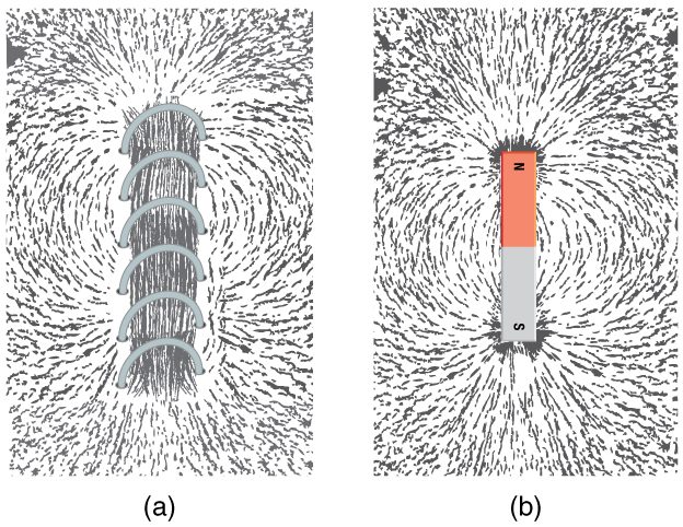
סליל המעביר זרם (סולנואיד) יוצר שדה מגנטי דומה בדיוק לשדה של מקטב מוטרב Vocabulary · מילון מונחים Train · אימוןEnglish עברית magnetic field/mæɡˈnetɪk fiːld/ שדה מגנטי vector field/ˈvektə fiːld/ שדה וקטורי magnetic field lines/mæɡˈnetɪk fiːld laɪnz/ קווי שדה מגנטי Maxwell's equations/ˈmækswelz ɪˈkweɪʒnz/ משוואות מקסוול magnetic monopoles/mæɡˈnetɪk ˈmɒnəʊpəʊlz/ מונופולים מגנטיים magnetic dipole/mæɡˈnetɪk ˈdaɪpəʊl/ דו-קוטב מגנטי compass/ˈkʌmpəs/ מצפן Ferromagnetic/ˌferəməɡˈnetɪk/ פרומגנטי magnetic domains/mæɡˈnetɪk dəˈmeɪnz/ תחומים מגנטיים Paramagnetic/ˌpærəməɡˈnetɪk/ פראמגנטי Diamagnetic/ˌdaɪəməɡˈnetɪk/ דיאמגנטי magnetic permeability/mæɡˈnetɪk ˌpɜːməˈbɪlɪti/ חדירות מגנטית perpendicular/ˌpɜːpənˈdɪkjʊlə/ ניצב centripetal force/senˈtrɪpɪtl fɔːs/ כוח צנטריפטלי velocity selector/vəˈlɒsɪti sɪˈlektə/ בוחן מהירות Hall effect/hɔːl ɪˈfekt/ אפקט הול Biot–Savart law/ˈbɪɒt ˈsævɑːt lɔː/ חוק ביו-סבאר tangent/ˈtændʒənt/ טנגנס concentric circles/kənˈsentrɪk ˈsɜːklz/ מעגלים קונצנטריים Ampère's law/ˈæmpeəz lɔː/ חוק אמפיר Amperian loop/æmˈpɪərɪən luːp/ לולאת אמפיר current density/ˈkʌrənt ˈdensɪti/ צפיפות זרם superposition/ˌsuːpəpəˈzɪʃn/ הפרעה (סופרפוזיציה) solenoid/ˈsəʊlənɔɪd/ סולנואיד 12.4
Ampère's Law · חוק אמפère
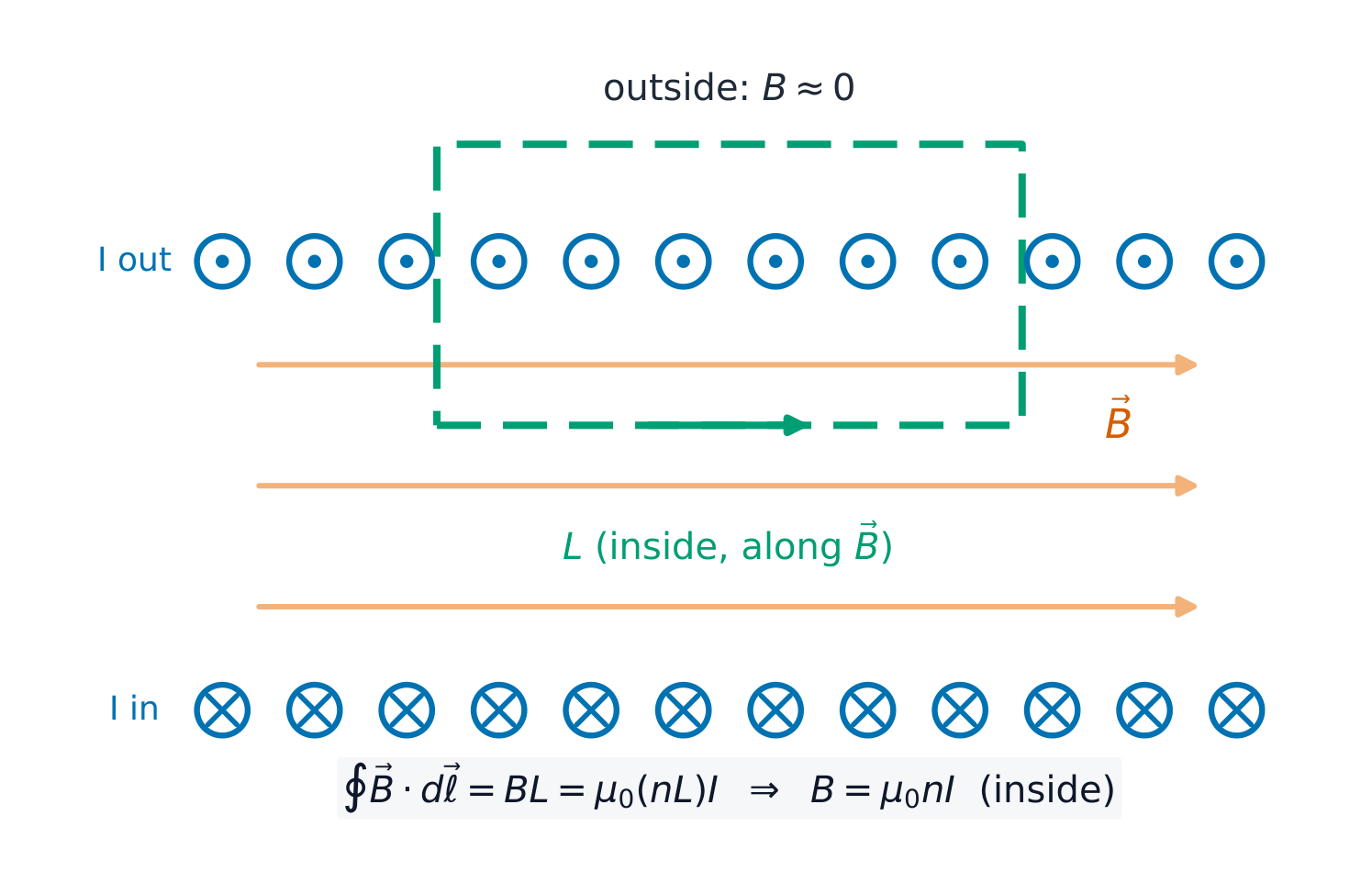
Syllabus · סיילבוס
EnglishLearning Objective 12.4.A: Use Ampère's law to describe the magnetic field created by a moving charge carrier.
- 12.4.A.1 Ampère's law relates the magnitude of the magnetic field to the current enclosed by a closed imaginary path called an Amperian loop.
- Equation: $\oint \vec{B} \cdot d\vec{\ell} = \mu_0 I_{\text{enc}}$
- 12.4.A.1.i Ampère's law can be used to determine the magnetic field near a long, straight current-carrying wire.
- Equation: $B_{\text{wire}} = \dfrac{\mu_0}{2\pi} \dfrac{I}{r}$
- 12.4.A.1.ii Unless otherwise stated, all solenoids are assumed to be very long, with uniform magnetic fields inside the solenoids and negligible magnetic fields outside the solenoids.
- 12.4.A.1.iii Ampère's law can be used to determine the magnetic field inside of a long solenoid.
- Equation: $B_{\text{sol}} = \mu_0 n I$
- 12.4.A.2 An Amperian loop is a closed path around a current-carrying conductor.
- 12.4.A.3 The principle of superposition can be used to determine the net magnetic field at a point in space created by various combinations of current-carrying conductors, or conducting loops, segments, or cylinders.
- 12.4.A.4 Maxwell's equations are the collection of equations that fully describe electromagnetism. Maxwell's fourth equation is Ampère's law with Maxwell's addition; it states that magnetic fields can be generated by electric current (Ampère's law) and that a changing electric field creates a magnetic field, similar to the way a moving charge creates a magnetic field (Maxwell's addition).
- Equation: $\oint \vec{B} \cdot d\vec{\ell} = \mu_0 I + \mu_0 \varepsilon_0 \dfrac{d\Phi_E}{dt}$
Boundary statement: AP Physics C: Electricity & Magnetism only expects quantitative application of Ampère's law limited to situations involving symmetrical magnetic fields. Long straight wires, long solenoids carrying currents, as well as conductive slabs or cylindrical conductors carrying a current density, are the types of shapes to which Ampère's law will be applied on the AP Physics C: Electricity & Magnetism Exam.
Boundary statement: AP Physics C: Electricity & Magnetism does not expect students to use Maxwell's fourth equation with a changing electric field. However, students should understand that a changing electric field generates a magnetic field.
עבריתמטרת הלמידה 12.4.A: להשתמש בחוק אמפר כדי לתאר את השדה המגנטי הנוצר על ידי נשיא מטען נע.
- 12.4.A.1 חוק אמפר מקשר בין גודל השדה המגנטי לבין הזרם הכלוא בתוך לולאה מדומית סגורה הנקראת לולאת אמפר.
- משוואה: $\oint \vec{B} \cdot d\vec{\ell} = \mu_0 I_{\text{enc}}$
- 12.4.A.1.i ניתן להשתמש בחוק אמפר כדי לקבוע את השדה המגנטי סביב חוט ישר וארוך נושא זרם.
- משוואה: $B_{\text{wire}} = \dfrac{\mu_0}{2\pi} \dfrac{I}{r}$
- 12.4.A.1.ii אלא אם כן צוין אחרת, כל הסולנוידים נחשבים לארוכים מאוד, עם שדות מגנטיים אחידים בתוך הסולנוידים ושדות מגנטיים זניחים מחוץ לסולנוידים.
- 12.4.A.1.iii ניתן להשתמש בחוק אמפר כדי לקבוע את השדה המגנטי בתוך סולנויד ארוך.
- משוואה: $B_{\text{sol}} = \mu_0 n I$
- 12.4.A.2 לולעת אמפר היא מסלול סגור סביב מוליך העובר בו זרם חשמלי.
- 12.4.A.3 ניתן להשתמש בעקרון הסופרפוזיציה כדי לקבוע את השדה המגנטי הכולל בנקודה כלשהי במרחב שנוצר על ידי שילובים שונים של מוליכים העוברים בהם זרמים, או לולאות הולכה, קטעים או צילינדרים.
- 12.4.A.4 משוואות מקסוול הן קבוצת המשוואות המתארת במלואה את האלקטרומגנטיות. משוואת מקסוול הרביעית היא חוק אמפר עם התוספת של מקסוול; היא קובעת כי שדות מגנטיים יכולים להיות נוצרים על ידי זרם חשמלי (חוק אמפר) וכי שדה חשמלי משתנה יוצר שדה מגנטי, בדומה לכך שטעינה נעה יוצרת שדה מגנטי (התוספת של מקסוול).
- משוואה: $\oint \vec{B} \cdot d\vec{\ell} = \mu_0 I + \mu_0 \varepsilon_0 \dfrac{d\Phi_E}{dt}$
הצהרת גבול: AP Physics C: חשמל ומגנטיות מצפה רק ליישום כמותי של חוק אמפר המוגבל למצבים המעורבים בשדות מגנטיים סימטריים. חוטים ישרים ארוכים, סולנוידים ארוכים העוברים בהם זרמים, כמו גם לוחות מוליכים או מוליכים צילינדריים העוברים בהם צפיפות זרם, הם סוגי הצורות אליהן ייושם חוק אמפר בבחינת AP Physics C: חשמל ומגנטיות.
הצהרת גבול: AP Physics C: חשמל ומגנטיות אינו מצפה מתלמידים להשתמש במשוואת מקסוול הרביעית עם שדה חשמלי משתנה. עם זאת, התלמידים צריכים להבין ששדה חשמלי משתנה מייצר שדה מגנטי.
Source: College Board AP Course and Exam Description · מקור: תיאור הקורס והמבחן של College Board AP
EnglishFor symmetric current distributions, Ampère's law 安培定律 finds the field far faster than Biot–Savart:
$$\oint \vec{B}\cdot d\vec{l}=\mu_0 I_{\text{enc}}.$$Choose an Amperian loop 安培环路 that matches the symmetry, so that $B$ is constant along the loop (and parallel to it) and comes out of the integral. AP applies it to long straight wires, long solenoids, and conductors carrying a current density 电流密度 (slabs and cylinders); combinations are handled by superposition 叠加.
Worked example. Find the field $0.10\ \text{m}$ from a long wire carrying $5.0\ \text{A}$. A circular loop of radius $r$ shares the field's symmetry, so $B(2\pi r)=\mu_0 I$ and
$$B=\frac{\mu_0 I}{2\pi r}=\frac{(4\pi\times10^{-7})(5.0)}{2\pi(0.10)}=1.0\times10^{-5}\ \text{T}.$$A long solenoid 螺线管 (assumed: uniform field inside, negligible field outside) is the other classic. Take a rectangular loop with one side of length $L$ inside, parallel to the axis: only that side contributes to the integral, so $BL=\mu_0 (nL) I$ and
$$B_{\text{sol}}=\mu_0 n I,$$with $n$ the turns per metre.
Worked example (cylinder). A solid cylindrical conductor of radius $R$ carries current $I$ spread uniformly over its cross-section. Inside ($r
Exam skill. Every Ampère's-law answer earns its marks in the setup: name the loop, state why $B$ is constant and parallel to it (symmetry), and count $I_{\text{enc}}$ carefully before you solve. Maxwell's fourth equation adds one more idea you should know qualitatively: a changing electric field also creates a magnetic field – but AP will not ask you to compute with that term.
עבריתלחלוקות זרם סימטריות, חוק אמפère מוצא את השדה הרבה מהר יותר מאשר ביוט-סבר:
$$\oint \vec{B}\cdot d\vec{l}=\mu_0 I_{\text{enc}}.$$בחרו מעגל אמפרי התואם את הסימטריה, כך ש$B$ יהיה קבוע לאורך המעגל (וחלקי ממנו) ויציא מהאינטגרל. AP משתמש בכך עבור חוטים ישרים ארוכים, סולנוידים ארוכים ומוליכים עם צפיפות זרם (לוחות וגלילים); שילובים טיפולים על ידי סופרפוזיציה.
דוגמה מופתרת. מצאו את השדה $0.10\ \text{m}$ מאורך חוט ארוך העובר בו $5.0\ \text{A}$. מעגל עגול ברדיוס $r$ משתף סימטריה זו של השדה, ולכן $B(2\pi r)=\mu_0 I$ ו
$$B=\frac{\mu_0 I}{2\pi r}=\frac{(4\pi\times10^{-7})(5.0)}{2\pi(0.10)}=1.0\times10^{-5}\ \text{T}.$$סליל ארוך (סולנויד) הוא הקלאסי השני (בהנחה: שדה אחיד בתוך, שדה זניח מחוץ). לקח לולאה מלבנית עם צד אחד באורך $L$ בתוך, מקביל לציר: רק צד זה תורם לאינטגרל, ולכן $BL=\mu_0 (nL) I$ ו
$$B_{\text{sol}}=\mu_0 n I,$$כאשר $n$ הוא מספר ההליכות למטר.
לולאת אמפère מלבנית גוזרת את השדה האחיד בתוך סליל דוגמה מפורטת (צילינדר). מוליך צילינדרי מוצק בעל רדיוס $R$ ועובר בו זרם $I$ המפוזר באופן אחיד על פני חתכו. בתוך ($r
מיומנות לבחינה. לכל תשובה בחוק אמפère יש להרוויח את נקודותיה בהגדרה: קרא את שם הלולאה, ציין למה $B$ קבוע ונאנך לה (סימטריה), וחשב בזהירות את $I_{\text{enc}}$ לפני שהפתרת. משוואת רביעית של מקסוול מוסיפה רעיון נוסף שחייבת לדעת באופן איכותי: שדה חשמלי משתנה גם הוא יוצר שדה מגנטי – אך AP לא יבקש ממך לחשב עם האיבר הזה.
12.4
Exam tips · טיפים לבחינות
English- The magnetic force $\vec F=q\vec v\times\vec B$ is perpendicular to velocity — use the right-hand rule and note it does no work.
- A charge in a uniform field moves in a circle with $r=\tfrac{mv}{qB}$.
- Find the field of currents with Biot–Savart $d\vec B=\tfrac{\mu_0}{4\pi}\tfrac{I\,d\vec l\times\hat r}{r^2}$ or Ampère's law $\oint \vec B\cdot d\vec l=\mu_0 I_{enc}$ when there is symmetry.
- Force on a wire is $\vec F=I\vec L\times\vec B$; keep the cross-product direction straight.
- Distinguish the force on a charge from the field the current creates.
עברית- הכוח המגנטי $\vec F=q\vec v\times\vec B$ הוא ניצב למהירות — השתמש בכלל היד הימנית והערה שהוא לא מבצע עבודה.
- מטען בשדה אחיד נע במסלול עגול עם $r=\tfrac{mv}{qB}$.
- מצא את שדה הזרמים עם ביוט-סבר $d\vec B=\tfrac{\mu_0}{4\pi}\tfrac{I\,d\vec l\times\hat r}{r^2}$ או חוק אמפère $\oint \vec B\cdot d\vec l=\mu_0 I_{enc}$ כאשר יש סימטריה.
- כוח על חוט הוא $\vec F=I\vec L\times\vec B$; שמור על כיוון מכפלת הצלב נכון.
- הבדל בין הכוח על מטען לבין השדה שהזרם יוצר.
- 12.1.A.1 A magnetic field is a vector field that can be used to determine the magnetic force exerted on moving electric charges, electric currents, or magnetic materials.
-
13
Electromagnetic Induction · השראה אלקטרומגנטית
Watch lesson · צפה בשיעור13.1
Magnetic Flux · זרימת מגנטים
Syllabus · סיילבוס
EnglishLearning Objective 13.1.A: Describe the magnetic flux through an arbitrary area or geometric shape.
- 13.1.A.1 For a magnetic field $\vec{B}$ that is constant across an area $\vec{A}$, the magnetic flux through the area is defined as $\Phi_B = \vec{B} \cdot \vec{A}$ .
- 13.1.A.1.i The area vector is defined as perpendicular to the plane of the surface and outward from a closed surface.
- 13.1.A.1.ii The sign of flux is given by the dot product of the magnetic field vector and the area vector.
- 13.1.A.2 The total magnetic flux passing through a surface is defined by the surface integral of the magnetic field over the surface area.
- Equation: $\Phi_B = \displaystyle\int \vec{B} \cdot d\vec{A}$
עבריתמטרת לימוד 13.1.A: לתאר את הפlux המגנטי דרך שטח או צורה גיאומטרית כלשהי.
- 13.1.A.1 עבור שדה מגנטי $\vec{B}$ הקבוע לאורך שטח $\vec{A}$, הפlux המגנטי דרך השטח מוגדר כ-$\Phi_B = \vec{B} \cdot \vec{A}$.
- 13.1.A.1.i וקטור השטח מוגדר כניצב למישור המשטח וחוצה אותו החוצה מפני שטח סגור.
- 13.1.A.1.ii סימן הפlux נתון על ידי מכפלת הנקודתית של וקטור השדה המגנטי ווקטור השטח.
- 13.1.A.2 הפlux המגנטי הכולל העובר דרך משטח מוגדר על ידי האיגרל השטחי של השדה המגנטי לאורך שטח המשטח.
- משוואה: $\Phi_B = \displaystyle\int \vec{B} \cdot d\vec{A}$
Source: College Board AP Course and Exam Description · מקור: תיאור הקורס והמבחן של College Board AP
EnglishMagnetic flux 磁通量 measures how much magnetic field passes through a surface. For a uniform field through a flat loop it is the dot product $\Phi_B=\vec{B}\cdot\vec{A}=BA\cos\theta$; in general it is the surface integral 面积分
$$\Phi_B=\int \vec{B}\cdot d\vec{A}.$$The area vector 面积矢量 is perpendicular to the surface (outward from a closed one), and the sign of the flux comes from the dot product. Flux changes if $B$ changes, the area changes, or the loop turns – keep all three routes in mind, because each one is an exam question.
עבריתזרימת מגנטים מדדת כמה שדה מגנטי עובר דרך משטח. עבור שדה אחיד דרך לולאה שטוחה זהו המכפלה הסקלרית $\Phi_B=\vec{B}\cdot\vec{A}=BA\cos\theta$; באופן כללי זו אינטגרל משטחי
$$\Phi_B=\int \vec{B}\cdot d\vec{A}.$$ווקטור השטח הוא ניצב למשטח (כלפי חוץ ממסגרת סגורה), ותוסיף הזרימה נובעת מהמכפלה הסקלרית. הזרימה משתנה אם $B$ משתנה, השטח משתנה, או הלולאה מתהפכת – שמור את שלושת הדרך במחשבה, כי כל אחת מהן היא שאלת בחינה.
13.2
Electromagnetic Induction · השראה אלקטרומגנטית
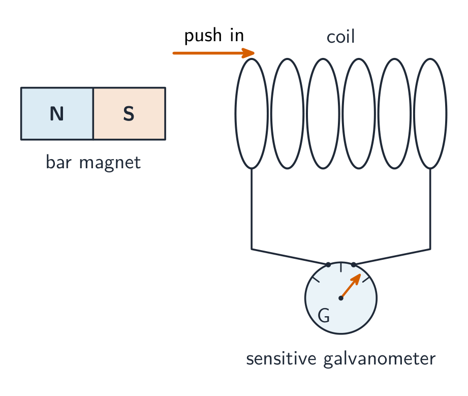
Syllabus · סיילבוס
EnglishLearning Objective 13.2.A: Describe the induced electric potential difference resulting from a change in magnetic flux.
- 13.2.A.1 Faraday's law describes the relationship between changing magnetic flux and the resulting induced emf in a system.
- Equation: $\mathcal{E} = -\dfrac{d\Phi_B}{dt} = -\dfrac{d\left(\vec{B} \cdot \vec{A}\right)}{dt}$
- 13.2.A.1.i When the area of the surface being considered is constant, the induced emf is equal to the area multiplied by the rate of change in the component of the magnetic field perpendicular to the surface.
- 13.2.A.1.ii When the magnetic field is constant, the induced emf is equal to the magnetic field multiplied by the rate of change in area perpendicular to the magnetic field.
- 13.2.A.1.iii When an emf is induced in a long solenoid, the total induced emf is equal to the induced emf in a single loop multiplied by the number of loops in the solenoid.
- Equation: $\left|\mathcal{E}_{\text{sol}}\right| = N\left|\dfrac{d\Phi_B}{dt}\right|$
- 13.2.A.2 Lenz's law is used to determine the direction of an induced emf resulting from a changing magnetic flux.
- 13.2.A.2.i An induced emf generates a current that creates a magnetic field that opposes the change in magnetic flux.
- 13.2.A.2.ii The right-hand rule is used to determine the relationships between current, emf, and magnetic flux.
- 13.2.A.3 Maxwell's equations are the collection of equations that fully describe electromagnetism. Maxwell's third equation is Faraday's law of induction, which describes the relationship between a changing magnetic flux and an induced electric field.
- Equation: $\mathcal{E} = \oint \vec{E} \cdot d\vec{\ell} = -\dfrac{d\Phi_B}{dt}$
- 13.2.A.4 Maxwell's equations can be used to show that electric and magnetic fields obey wave equations and that electromagnetic waves travel at a constant speed in free space.
- Equation (derived): $c = \dfrac{1}{\sqrt{\varepsilon_0 \mu_0}}$
Boundary statement: AP Physics C: Electricity & Magnetism does not expect students to mathematically derive the speed of light in free space from Maxwell's equations. This relationship is included above solely as an indication of the further applications, implications, and connections to physical phenomena that students may study in more advanced physics courses.
עבריתמטרת לימוד 13.2.A: לתאר את הפרש הפוטנציאל החשמלי המושרה הנובע משינוי בפflux המגנטי.
- 13.2.A.1 חוק פראדיי מתאר את הקשר בין שינוי בפflux המגנטי לבין ה-EMF המושרה בתוצאתו במערכת.
- משוואה: $\mathcal{E} = -\dfrac{d\Phi_B}{dt} = -\dfrac{d\left(\vec{B} \cdot \vec{A}\right)}{dt}$
- 13.2.A.1.i כאשר שטח המשטח הנבחן הוא קבוע, ה-EMF המושרה שווה לשטח כפול קצב השינוי ברכיב השדה המגנטי הניצב למשטח.
- 13.2.A.1.ii כאשר השדה המגנטי קבוע, ה-EMF המושרה שווה לשדה המגנטי כפול קצב השינוי בשטח הניצב לשדה המגנטי.
- 13.2.A.1.iii כאשר EMF מושרד בסולנויד ארוך, ה-EMF המושרה הכולל שווה ל-EMF המושרד בלולאה אחת כפול מספר הלולאות בסולנויד.
- משוואה: $\left|\mathcal{E}_{\text{sol}}\right| = N\left|\dfrac{d\Phi_B}{dt}\right|$
- 13.2.A.2 חוק לנץ משמש לקביעת הכיוון של ה-EMF המושרה הנובע משינוי בפflux המגנטי.
- 13.2.A.2.i EMF מושרד מייצר זרם היוצר שדה מגנטי הנגד לשינוי בפflux המגנטי.
- 13.2.A.2.ii כלל היד הימנית משמש לקביעת הקשרים בין זרם, EMF ופflux מגנטי.
- 13.2.A.3 משוואות מקסוול הן קבוצת המשוואות המתארת במלואה את האלקטרומגנטיות. משוואה שלישית של מקסוול היא חוק האינדוקציה של פאראדי, המתאר את הקשר בין שינוי בשיטת השדה המגנטי לשדה חשמלי מופעל.
- משוואה: $\mathcal{E} = \oint \vec{E} \cdot d\vec{\ell} = -\dfrac{d\Phi_B}{dt}$
- 13.2.A.4 ניתן להשתמש במשוואות מקסוול כדי להראות שהשדות החשמליים והמגנטיים עומדים במשוואות גל, ושגלים אלקטרומגנטיים נעים במהירות קבועה בחלל ריק.
- משוואה (מובקעת): $c = \dfrac{1}{\sqrt{\varepsilon_0 \mu_0}}$
ניסוח לגבול: AP Physics C: חשמל ומגנטיות אינה מצפה מתלמידים לבצע נגזרות מתמטיות למהירות האור בחלל ריק מתוך משוואות מקסוול. קשר זה כלול לעיל רק כהמחשה של יישומים, השפעות וקשרים נוספים לתופעות פיזיקליות שבהם התלמידים עשויים ללמוד בקורסי פיזיקה מתקדמים יותר.
Source: College Board AP Course and Exam Description · מקור: תיאור הקורס והמבחן של College Board AP
EnglishElectromagnetic induction A changing flux induces an emf 电动势 – Faraday's law 法拉第定律:
$$\varepsilon=-\frac{d\Phi_B}{dt}.$$With constant area, $\varepsilon=-A\,\dfrac{dB_\perp}{dt}$; with constant field, $\varepsilon=-B\,\dfrac{dA_\perp}{dt}$. A coil of $N$ turns multiplies the single-loop emf: $|\varepsilon_{\text{sol}}|=N\left|\dfrac{d\Phi_B}{dt}\right|$.
Lenz's law 楞次定律 is the minus sign: the induced current 感应电流 flows so that its own magnetic field opposes the change in flux that created it. Push a magnet toward a loop and the loop pushes back; pull it away and the loop pulls it in. Use the right-hand rule 右手定则 to turn "oppose the change" into a current direction.
A rod of length $L$ sliding at speed $v$ across a field is the special case worth memorising – the motional emf 动生电动势 $\varepsilon=BLv$.
Worked example. A $0.20\ \text{m}$ rod slides at $3.0\ \text{m/s}$ across a $0.50\ \text{T}$ field: $\varepsilon=BLv=0.50(0.20)(3.0)=0.30\ \text{V}$. Equivalently, if a single loop's flux drops from $0.020\ \text{Wb}$ to $0.008\ \text{Wb}$ in $0.030\ \text{s}$, the average emf is $\varepsilon=\dfrac{0.012}{0.030}=0.40\ \text{V}$.
Faraday's law is also the third of Maxwell's equations 麦克斯韦方程组, in a deeper form: a changing magnetic flux creates a circulating electric field, $\oint\vec{E}\cdot d\vec{l}=-\dfrac{d\Phi_B}{dt}$ – that field is what pushes the charges around the loop. Together, Maxwell's equations predict electromagnetic waves 电磁波 travelling at $c=1/\sqrt{\varepsilon_0\mu_0}$ (you should know this connection, but AP will not ask you to derive it).
עבריתהשראת אלקטרומגנטית שינוי בזרימת השדה גורם להופעת המ"ע – חוק פאראדי:
$$\varepsilon=-\frac{d\Phi_B}{dt}.$$עם שטח קבוע, $\varepsilon=-A\,\dfrac{dB_\perp}{dt}$; עם שדה קבוע, $\varepsilon=-B\,\dfrac{dA_\perp}{dt}$. סליל בעל $N$ הליכות מכפיל את ה-EMF של לולאה אחת: $|\varepsilon_{\text{sol}}|=N\left|\dfrac{d\Phi_B}{dt}\right|$.
חוק לנץ הוא סימן החסר: הזרם המושפע זורם כך שהשדה המגנטי שלו מונע את השינוי בזרימה שיצר אותו. דוחפים מגנט לעבר לולאה והלולאה דוחפת בחזרה; משלחים אותו והלולאה מושכת אותו פנימה. השתמשו בכלל היד הימנית כדי להפוך "להנגד את השינוי" לכיוון הזרם.
זוזת מקטב לתוך סליל מופעת כוח אלקטרו-מניעי (e.m.f.) שמדריך זרם מוט באורך $L$ הנע במהירות $v$ בשדה הוא המקרה הפרטי ששווה לשנן – ההמ"ע תנועה $\varepsilon=BLv$.
דוגמה מפורטת. מוט $0.20\ \text{m}$ נע במהירות $3.0\ \text{m/s}$ בשדה $0.50\ \text{T}$: $\varepsilon=BLv=0.50(0.20)(3.0)=0.30\ \text{V}$. באופן שקול, אם זרימת לולאה אחידה יורדת מ$0.020\ \text{Wb}$ ל$0.008\ \text{Wb}$ בתוך $0.030\ \text{s}$, ההמ"ע הממוצעת היא $\varepsilon=\dfrac{0.012}{0.030}=0.40\ \text{V}$.
חוק פאראדי הוא גם השלישי במשוואות מקסוול, בצורה עמוקה יותר: זרימה מגנטית משתנה יוצרת שדה חשמלי מסתובב, $\oint\vec{E}\cdot d\vec{l}=-\dfrac{d\Phi_B}{dt}$ – שדה זה הוא מה שמדחוף את המטענים סביב הלולאה. ביחד, משוואות מקסוול חוזה גלי אלקטרומגנטיים הנעים במהירות $c=1/\sqrt{\varepsilon_0\mu_0}$ (אתם צריכים לדעת קשר זה, אך AP לא יבקש ממכם להוכיח אותו).
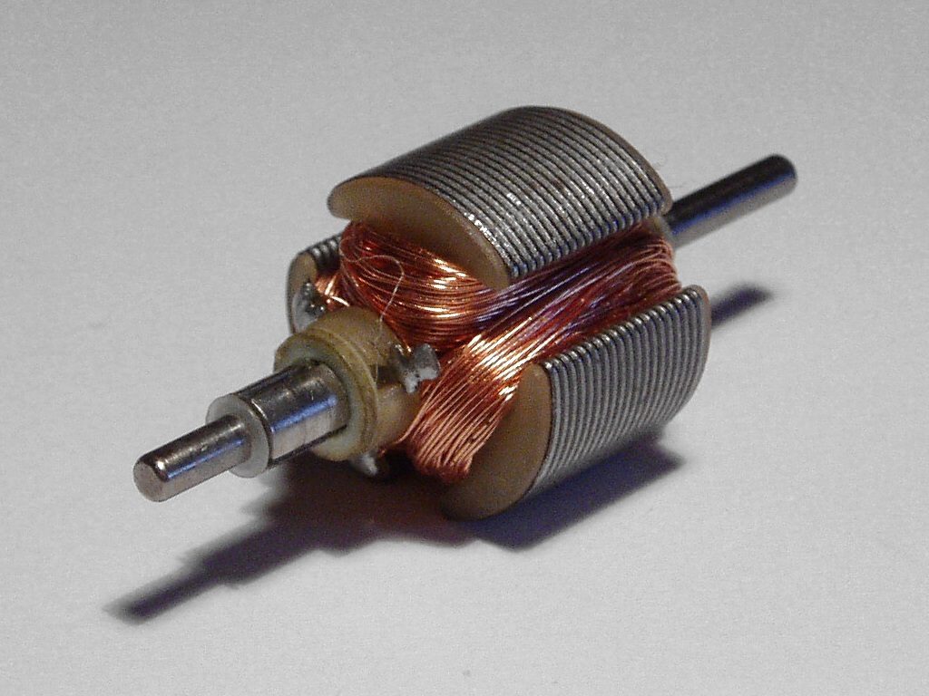
סלילי חוט מסתובבים בשדה מגנטי: הזזתם בשדה גורמים להופעת זרם, זו הבסיס לגנרטור 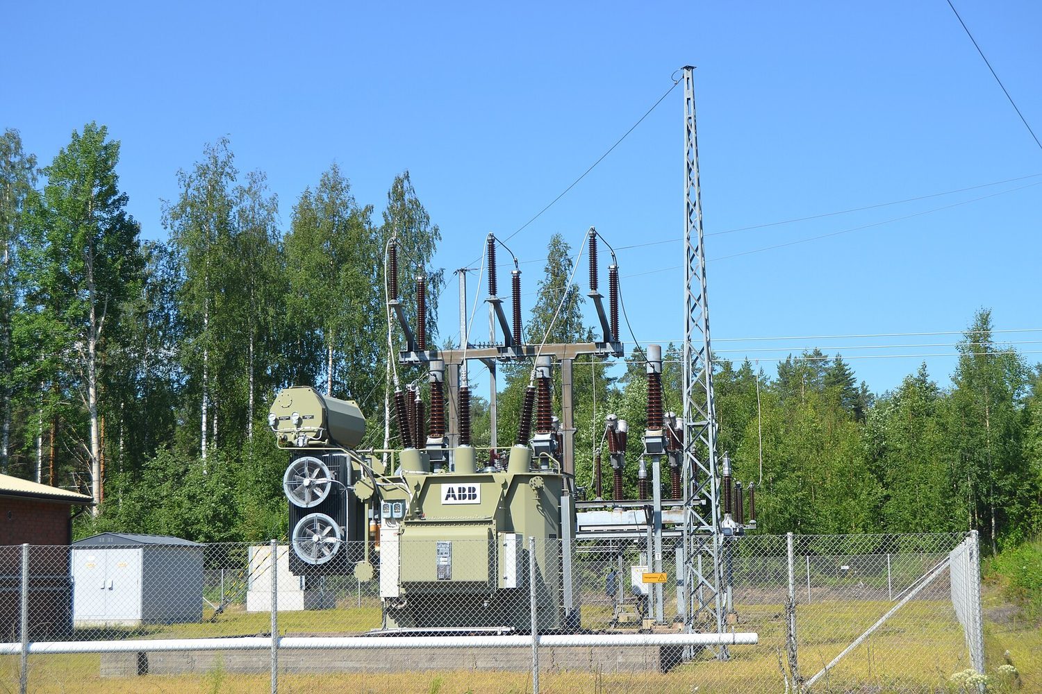
מתחנת חשמל: הזרם המגנטי המשתנה בסלילים מופע את המתחים המספקים חשמל לרשת Explore · חקורInduce a current by moving a magnet · להפעיל זרם על ידי הזזת מגנט
A changing magnetic flux through a coil induces an EMF (Faraday's law); its direction opposes the change (Lenz's law). Move the magnet faster for a bigger EMF. · שינוי בשטף מגנטי דרך סליל מעורר כוח חשמלי (חוק פארادאי); כיוונו מתנגד לשינוי (חוק לנץ). הזזת המגנט מהר יותר תניב כוח חשמלי גדול יותר.
Vocabulary · מילון מונחים Train · אימוןEnglish עברית Magnetic flux/mæɡˈnetɪk flʌks/ השטף המגנטי surface integral/ˈsɜːfɪs ˈɪntɪɡrəl/ אינטגרל פני שטח area vector/ˈeərɪə ˈvektə/ ווקטור שטח emf/emf/ כוח חשמלי Faraday's law/ˈfærədeɪz lɔː/ חוק פאראדיי Lenz's law/ˈlentsɪz lɔː/ חוק לנץ induced current/ɪnˈdjuːst ˈkʌrənt/ זרם מושרה right-hand rule/raɪt hænd ruːl/ כלל היד ימין motional emf/ˈməʊʃənl emf/ כוח חשמלי תנועתי Maxwell's equations/ˈmækswelz ɪˈkweɪʒnz/ משוואות מקסוול electromagnetic waves/ɪˌlektrəʊməɡˈnetɪk weɪvz/ גלים אלקטרומגנטיים eddy currents/ˈedi ˈkʌrənts/ זרמי עורף generator/ˈdʒenəreɪtə/ גנרטור inductance/ɪnˈdʌktəns/ עצמת השראה inductor/ɪnˈdʌktə/ סולנואיד solenoid/ˈsəʊlənɔɪd/ סולנואיד magnetic permeability/mæɡˈnetɪk ˌpɜːməˈbɪlɪti/ חדירות מגנטית RL circuit/ˌɑː ˈel ˈsɜːkɪt/ מעגל RL differential equation/ˌdɪfəˈrenʃl ɪˈkweɪʒn/ משוואה דיפרנציאלית time constant/taɪm ˈkɒnstənt/ קבוע זמן LC circuit/ˌel ˈsiː ˈsɜːkɪt/ מעגל LC oscillates/ˈɒsɪleɪts/ מתנודדת simple harmonic motion/ˈsɪmpl hɑːˈmɒnɪk ˈməʊʃn/ תנועה הרמונית פשוטה conservation of energy/ˌkɒnsəˈveɪʃn ɒv ˈenədʒi/ שימור אנרגיה 13.3
Induced Currents and Magnetic Forces · זרמים מושעים וכוחות מגנטיים
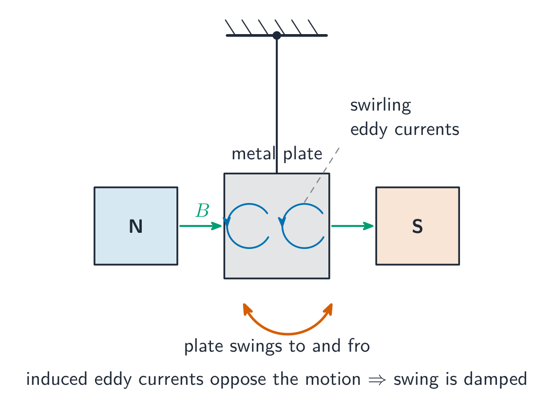
Syllabus · סיילבוס
EnglishLearning Objective 13.3.A: Describe the force exerted on a conductor due to the interaction between an external magnetic field and an induced current within that conductor.
- 13.3.A.1 When an induced current is created in a conductive loop, the already-present magnetic field will exert a magnetic force on the moving charge carriers within the loop.
- Equation: $\vec{F}_B = \displaystyle\int I\left(d\vec{\ell} \times \vec{B}\right)$
- 13.3.A.2 When current is induced in a conducting loop, magnetic forces are only exerted on the segments of the loop that are within the external magnetic field. These magnetic forces may cause translational or rotational acceleration.
- 13.3.A.3 The force on a conducting loop is proportional to the induced current in the loop, which depends on the rate of change of magnetic flux, the resistance of the loop, and the velocity of the loop.
- 13.3.A.4 Newton's second law can be applied to a conducting loop moving in a magnetic field as it experiences an induced emf.
עבריתמטרות למידה 13.3.A: תאר את הכוח הפועל על מוליך בשל האינטראקציה בין שדה מגנטי חיצוני לזרם מופעל בתוך המוליך.
- 13.3.A.1 כאשר נוצר זרם מופעל בטבעת מוליכה, השדה המגנטי הקיים יפעיל כוח מגנטי על נשיאי המטען הנעים בתוך הטבעת.
- משוואה: $\vec{F}_B = \displaystyle\int I\left(d\vec{\ell} \times \vec{B}\right)$
- 13.3.A.2 כאשר זרם מופעל בטבעת מוליכה, כוחות מגנטיים פועלים רק על המקטעים של הטבעת הנמצאים בתוך השדה המגנטי החיצוני. כוחות מגנטיים אלו עשויים לגרום להאצה תרגולית או סיבובית.
- 13.3.A.3 הכוח הפועל על טבעת מוליכה פרופורציונלי לזרם המופעל בה, התלוי בקצב השינוי בשיטת השדה המגנטי, ההתנגדות של הטבעת ובמהירות הטבעת.
- 13.3.A.4 ניתן להחיל את חוק השני של ניוטון על טבעת מוליכה הנעה בשדה מגנטי בעת חוויתה EMF מופעל.
Source: College Board AP Course and Exam Description · מקור: תיאור הקורס והמבחן של College Board AP
EnglishOnce an induced current flows, the external field exerts forces on it ($\vec{F}=\int I\,d\vec{l}\times\vec{B}$) – and by Lenz's law those forces always resist the motion that causes the induction. Only the segments of the loop actually inside the field feel a force, which can make a loop accelerate, rotate, or brake. This is the origin of eddy currents 涡电流 braking, and you can apply Newton's second law to a moving loop or rod like any other mechanics problem.
The classic setup is a rod sliding on conducting rails connected by a resistor:
Worked example (the full chain). Rails $L=0.20\ \text{m}$ apart with resistance $R=0.60\ \Omega$ sit in a $0.50\ \text{T}$ field into the page. The rod is pushed at a constant $3.0\ \text{m/s}$. Then: $\varepsilon=BLv=0.30\ \text{V}$; $I=\varepsilon/R=0.50\ \text{A}$; the field pushes back on the rod with $F=BIL=0.50(0.50)(0.20)=0.050\ \text{N}$. The pushing force does work at $P=Fv=0.15\ \text{W}$ – exactly the $P=I^2R=0.15\ \text{W}$ dissipated in the resistor. Mechanical work becomes electrical energy: that is a generator 发电机, and energy is conserved. Released with no push, the rod slows exponentially: $ma=-\dfrac{B^2L^2}{R}v$.
Exam skill. FRQs walk this exact chain: flux $\to$ emf $\to$ current $\to$ force $\to$ Newton's second law. Write each link separately and check the direction with Lenz's law at the end.
עבריתברגע שעובר זרם מושע, השדה החיצוני מפעיל כוחות עליו ($\vec{F}=\int I\,d\vec{l}\times\vec{B}$) – ובשל חוק לנץ, כוחות אלו תמיד מונעים את התנועה שגרמה להשעה. רק הקטעים של הלולאה שנמצאים בפועל בתוך השדה מרגישים בכוח, ודבר יכול לגרום ללולאה להאיץ, לסובב או לבלום. זוהי העלילה של בלמי זרמים עוקפיים, וניתן לחשב את חוק ניוטון השני עבור לולאה או מוט נעים כמו כל בעיה אחרת במכניקה.
ההתקן הקלאסי הוא מוט החולק על מסילות מוליכות המחוברות על ידי נגד:ההרכבה הקלאסית היא מוט הנע על מסילות מוליכות המחוברות באמצעות נגד:

מוט הנע על מסילות: הזרם המושע מרגיש בכוח המנוגד לתנועה דוגמה מפורטת (השרשרת המלאה). מסילות $L=0.20\ \text{m}$ מרחוק זה מזה עם התנגדות $R=0.60\ \Omega$ נמצאות בשדה $0.50\ \text{T}$ הפונה לתוך הדף. המוט נדחף במהירות קבועה $3.0\ \text{m/s}$. אז: $\varepsilon=BLv=0.30\ \text{V}$; $I=\varepsilon/R=0.50\ \text{A}$; השדה דוחף בחזרה על המוט בכוח של $F=BIL=0.50(0.50)(0.20)=0.050\ \text{N}$. כוח הדחיפה מבצע עבודה בקצב $P=Fv=0.15\ \text{W}$ – בדיוק ה$P=I^2R=0.15\ \text{W}$ המבוזר בנגד. עבודה מכנית הופכת לאנחיה חשמלית: זהו גנרטור, ואנחיה שמורה. אם משחררים אותו ללא דחיפה, המוט מאט באופן אקספוננציאלי: $ma=-\dfrac{B^2L^2}{R}v$.
מיומנות למבחן. FRQs עוברים על אותה שרשרת בדיוק: זרימה $\to$ המ"ע $\to$ זרם $\to$ כוח $\to$ חוק ניוטון השני. כתבו כל קשר בנפרד ובדקו את הכיוון עם חוק לנץ בסוף.
13.4
Inductance · אינדוקטיביות
Syllabus · סיילבוס
EnglishLearning Objective 13.4.A: Describe the physical and electrical properties of an inductor.
- 13.4.A.1 Inductance is the tendency of a conductor to oppose a change in electrical current.
- 13.4.A.1.i Inductance of a conductor depends on the physical properties of the conductor. Straight wires are typically modeled as having zero inductance.
- 13.4.A.1.ii An inductor, such as a solenoid, is a circuit element that has significant inductance.
- 13.4.A.1.iii The inductance of a solenoid is dependent on the total number of turns, the length of the solenoid, the cross-sectional area of the solenoid, and magnetic permeability of the solenoid's core.
- Equation: $L_{\text{sol}} = \dfrac{\mu_{\text{core}} N^2 A}{\ell}$
- 13.4.A.2 Inductors store energy in the magnetic field that is generated by current in the inductor.
- Equation: $U_L = \dfrac{1}{2} L I^2$
- 13.4.A.2.i The energy stored in the magnetic field generated by an inductor in which current is flowing can be dissipated through a resistor or used to charge a capacitor.
- 13.4.A.2.ii The transfer of energy generated in an inductor to other forms of energy obeys conservation laws.
- 13.4.A.3 By applying Faraday's law to an inductor and using the definition of inductance, induced emf can be related to inductance and the rate of change of current.
- Equation: $\mathcal{E}_i = -L\dfrac{dI}{dt}$
עבריתמטרות למידה 13.4.A: תאר את המאפיינים הפיזיקליים והחשמליים של סליל השראה.
- 13.4.A.1 השראה היא הנטייה של מוליך להתנגד לשינוי בזרם חשמלי.
- 13.4.A.1.i השראה של מוליך תלויה במאפיינים הפיזיקליים שלו. חוטים ישרים מתודגמים בדרך כלל כבעלי השראה אפסית.
- 13.4.A.1.ii סליל השראה, כמו סולנויד, הוא אלמנט מעגל חשמלי בעל השראה משמעותית.
- 13.4.A.1.iii השראה של סולנויד תלויה בסך הכל מסלילים, באורך הסולנויד, בשטח החתך שלו ובמחזוריות המגנטית (Permeability) של ליבת הסולנויד.
- משוואה: $L_{\text{sol}} = \dfrac{\mu_{\text{core}} N^2 A}{\ell}$
- 13.4.A.2 סלילי השראה מאחסנים אנרגיה בשדה המגנטי שנוצר על ידי הזרם בסליל.
- משוואה: $U_L = \dfrac{1}{2} L I^2$
- 13.4.A.2.i האנרגיה הארוזה בשדה המגנטי שנוצר על ידי סליל השראה דרך זורם בו יכולה להיות מפוזרת דרך נגד או משמשת לטעינת קבל.
- 13.4.A.2.ii העברת האנרגיה שנוצרה בסליל השראה לצורות אנרגיה אחרות עומדת בחוקי השימור.
- 13.4.A.3 על ידי היישום של חוק פאראדי לסליל השראה ובשימוש בהגדרת ההשראה, ניתן לקשר את ה-EMF המופעל להשראה ולקצב השינוי בזרם.
- משוואה: $\mathcal{E}_i = -L\dfrac{dI}{dt}$
Source: College Board AP Course and Exam Description · מקור: תיאור הקורס והמבחן של College Board AP
EnglishInductance 电感 is a conductor's tendency to oppose a change in its own current: changing current changes its own flux, which self-induces an emf. From Faraday's law,
$$\varepsilon=-L\frac{dI}{dt}.$$An inductor 电感器 is a circuit element built to have large inductance – usually a solenoid 螺线管, where geometry gives
$$L_{\text{sol}}=\frac{\mu_{\text{core}}N^2A}{\ell},$$with $N$ total turns, area $A$, length $\ell$, and the magnetic permeability 磁导率 of the core. (Straight wires are modelled as having zero inductance.) An inductor carrying current $I$ stores energy in its magnetic field:
$$U_L=\tfrac{1}{2}LI^2,$$which can later be dissipated in a resistor or moved into a capacitor – conservation of energy applies as usual.
עבריתאינדוקטיביות היא נטייתו של מוליך להתנגד לשינוי בזרם שלו: זרם משתנה משנה את הזרימה שלו, וזה גורם להופעת המ"ע עצמית. ממשוואת פאראדי,
$$\varepsilon=-L\frac{dI}{dt}.$$סליל הוא רכיב במעגל חשמלי המיועד להפיק אינדוקטוריות גבוהות – בדרך כלל סולנויד, שבו הגיאומטריה נותנת
$$L_{\text{sol}}=\frac{\mu_{\text{core}}N^2A}{\ell},$$עם $N$ הליכוד כולל, שטח $A$, אורך $\ell$ ונבילות מגנטית של ליבת הסליל. (חוטים ישרים מודלים כאילו יש להם אינדוקטוריות אפס.) סליל העובר בו זרם $I$ מאחסן אנרגיה בשדה המגנטי שלו:
$$U_L=\tfrac{1}{2}LI^2,$$שהיא יכולה להתפרק מאוחר יותר בתנגדות או לעבור לקבל – חוק שימור האנרגיה חל כרגיל.
13.5
Circuits with Resistors and Inductors · מעגלים עם תנגדות וסליבים
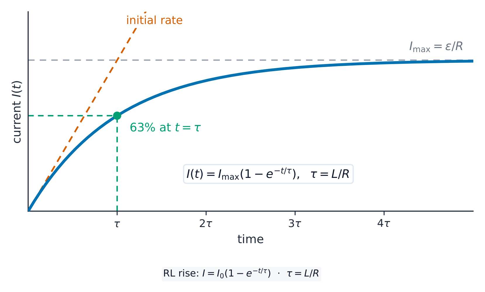
Syllabus · סיילבוס
EnglishLearning Objective 13.5.A: Describe the physical and electrical properties of a circuit containing a combination of resistors and a single inductor.
- 13.5.A.1 A resistor will dissipate energy that was stored in an inductor as the current changes.
- 13.5.A.2 Kirchhoff's loop rule can be applied to a series LR circuit with a battery of emf $\mathcal{E}$, resulting in a differential equation that describes the current in the loop.
- Equation (derived): $\mathcal{E} = IR + L\dfrac{dI}{dt}$
- 13.5.A.3 The time constant is a significant feature of the behavior of an LR circuit.
- 13.5.A.3.i The time constant of a circuit is a measure of how quickly an LR circuit will reach a steady state and is described with the equation $\tau = \dfrac{L}{R_{\text{eq}}}$ .
- 13.5.A.3.ii The time constant represents the time an LR circuit would take to reach a steady state if the system continued to change at the initial rate of change.
- 13.5.A.3.iii For an inductor that has zero initial current, the time constant represents the time required for the current in the inductor to reach approximately 63 percent of its final asymptotic value.
- 13.5.A.3.iv For an inductor with an initial current, the time constant represents the time required for the current in the inductor to reach approximately 37 percent of its initial value.
- 13.5.A.4 The electric properties of inductors change during the time interval in which the current in the inductor changes, but will exhibit steady state behavior after a long time interval.
- 13.5.A.4.i When a switch is initially closed or opened in a circuit containing an inductor, the induced emf will be equal in magnitude and opposite in direction to the applied potential difference across the branch containing the inductor.
- 13.5.A.4.ii The potential difference across an inductor, the current in the inductor, and the energy stored in the inductor are exponential with respect to time and have asymptotes that are determined by the initial conditions of the circuit.
- 13.5.A.4.iii After a time much greater than the time constant of the circuit, an inductor will behave as a conducting wire with zero resistance.
עבריתמטרות למידה 13.5.A: תאר את התכונות הפיזיקליות והחשמליות של מעגל המכיל שילוב של נגדים וסולנואיד אחד.
- 13.5.A.1 נגד יפזר אנרגיה שהתאגרה בסולנואיד כאשר הזורם משתנה.
- 13.5.A.2 ניתן ליישם את חוק הלולאה של קירכוף על מעגל LR סריתי עם מקור כוח $\mathcal{E}$, מה שמוביל למשוואה דיפרנציאלית המתארת את הזורם במעגל.
- משוואה (מובקעת): $\mathcal{E} = IR + L\dfrac{dI}{dt}$
- 13.5.A.3 זמן האופיין הוא מאפיין משמעותי בהתנהגותו של מעגל LR.
- 13.5.A.3.i זמן האופיין של מעגל הוא מדד לכמה מהר מעגל LR יגיע למצב יציב, ומתואר באמצעות המשוואה $\tau = \dfrac{L}{R_{\text{eq}}}$.
- 13.5.A.3.ii זמן האופיין מייצג את הזמן שעבר מעגל LR כדי להגיע למצב יציב, אם המערכת הייתה ממשיכה לשנות עצמה בקצב השינוי ההתחלתי.
- 13.5.A.3.iii עבור סולנואיד בעל זורם התחלתי אפס, זמן האופיין מייצג את הזמן הנדרש כדי שהזורם בסולנואיד יגיע לכ-63 אחוזים מערכו האסימפטוטי הסופי.
- 13.5.A.3.iv עבור סולנואיד עם זורם התחלתי, זמן האופיין מייצג את הזמן הנדרש כדי שהזורם בסולנואיד יגיע לכ-37 אחוזים מערכו ההתחלתי.
- 13.5.A.4 התכונות החשמליות של סולנואידים משתנות במהלך פרק הזמן בו הזורם בהם משתנה, אך יציגו התנהגות מצב יציב לאחר פרק זמן ארוך.
- 13.5.A.4.i כאשר מתג נסגר או נפתח בתחילה במעגל המכיל סולנואיד, ה-EMF המיוצר יהיה שווה בגודלו והפוך בכיוונו לגבי ההפרש הפוטנציאלי המופעל על הענף המכיל את הסולנואיד.
- 13.5.A.4.ii ההפרש הפוטנציאלי על פני סולנואיד, הזורם בסולנואיד והאנרגיה האגורה בו הם פונקציות מעריכיות ביחס לזמן ויש להן אסימפטות הקבועות על ידי תנאי ההתחלה של המעגל.
- 13.5.A.4.iii לאחר זמן הגדול משמעותית מזמן האופיין של המעגל, סולנואיד יתנהג כמו חוט מוליך בעל התנגדות אפס.
Source: College Board AP Course and Exam Description · מקור: תיאור הקורס והמבחן של College Board AP
EnglishIn an RL circuit RL电路, Kirchhoff's loop rule for a battery $\varepsilon$, resistor $R$, and inductor $L$ in series gives a differential equation 微分方程:
$$\varepsilon=IR+L\frac{dI}{dt}\quad\Rightarrow\quad I(t)=\frac{\varepsilon}{R}\big(1-e^{-t/\tau}\big),\qquad \tau=\frac{L}{R}.$$The time constant 时间常数 $\tau$ sets the pace: after one $\tau$ a rising current reaches about $63\%$ of its final value (a decaying one falls to $37\%$); it is also how long the change would take at the initial rate. Learn the two limits – they answer most conceptual questions:
- Just after the switch closes ($t=0$): current cannot jump, so the inductor momentarily blocks it, self-inducing an emf equal and opposite to the applied potential difference.
- Long after ($t\gg\tau$): the current is steady, $dI/dt=0$, and the inductor behaves as a plain wire – the exact opposite of a capacitor.
Worked example. $\varepsilon=12\ \text{V}$, $R=6.0\ \Omega$, $L=3.0\ \text{H}$: final current $\varepsilon/R=2.0\ \text{A}$, $\tau=L/R=0.50\ \text{s}$. At $t=0.50\ \text{s}$ the current is $2.0(1-e^{-1})\approx1.3\ \text{A}$. At $t=0$ the inductor's potential difference is the full $12\ \text{V}$; as $t\to\infty$ it falls to zero. Current, inductor voltage, and stored energy are all exponential in time.
עבריתבמעגל RL RL, חוק לולאת קירשוף לסוללה $\varepsilon$, תנגדות $R$ וסליל $L$ בסדר נותן משוואה דיפרנציאלית:
$$\varepsilon=IR+L\frac{dI}{dt}\quad\Rightarrow\quad I(t)=\frac{\varepsilon}{R}\big(1-e^{-t/\tau}\big),\qquad \tau=\frac{L}{R}.$$ה-קבוע הזמן $\tau$ קובע את הקצב: לאחר זמן $\tau$ אחד, זרם עולה מגיע לכ-$63\%$ מהערך הסופי שלו (זרם דועה יורד ל-$37\%$); זה גם הזמן שהשינוי היה לוקח בקצב ההתחלתי. למדו את שני הגבולות – הם עונים על רוב השאלות הקונספטואליות:
- מיד אחרי סגירת המתג ($t=0$): הזרם לא יכול לקפוץ, ולכן הסליל חוסם אותו לרגע, ומייצר EMF עצמי שווה והפוך לפוטנציאל המופעל.
- לאחר זמן רב ($t\gg\tau$): הזרם יציב, $dI/dt=0$, והסליל מתנהג כמו חוט פשוט – בדיוק ההפך מקבל.
הזרם במעגל RL עולה אקספוננציאלית, ומגיע ל-63% בזמן קבוע אחד דוגמה מופתרת. $\varepsilon=12\ \text{V}$, $R=6.0\ \Omega$, $L=3.0\ \text{H}$: זרם סופי $\varepsilon/R=2.0\ \text{A}$, $\tau=L/R=0.50\ \text{s}$. ב$t=0.50\ \text{s}$ הזרם הוא $2.0(1-e^{-1})\approx1.3\ \text{A}$. ב$t=0$ הפרש הפוטנציאלים של הסליל הוא כולו $12\ \text{V}$; כאשר $t\to\infty$ הוא צומח לאפס. הזרם, מתח הסליל והאנרגיה המאוגרת הם כולם פונקציות אקספוננציאליות בזמן.
13.6
Circuits with Capacitors and Inductors · מעגלים עם קבלים וסליבים
Syllabus · סיילבוס
EnglishLearning Objective 13.6.A: Describe the physical and electrical properties of a circuit containing a combination of capacitors and a single inductor.
- 13.6.A.1 In circuits containing only a charged capacitor and an inductor (LC circuits), the maximum current in the inductor can be determined using conservation of energy within the circuit.
- 13.6.A.2 In LC circuits, the time dependence of the charge stored in the capacitor can be modeled as simple harmonic motion.
- Equation (derived): $\dfrac{d^2 q}{dt^2} = -\dfrac{1}{LC} q$
- 13.6.A.3 The angular frequency of an oscillating LC circuit can be derived from the differential equation that describes an LC circuit.
- Equation (derived): $\omega = \dfrac{1}{\sqrt{LC}}$
עבריתמטרות למידה 13.6.A: תאר את התכונות הפיזיקליות והחשמליות של מעגל המכיל שילוב של קבלים וסולנואיד אחד.
- 13.6.A.1 במעגלים המכילים רק קבל מטעון וסולנואיד (מעגלי LC), ניתן לחשב את הזורם המקסימלי בסולנואיד באמצעות שימור האנרגיה בתוך המעגל.
- 13.6.A.2 במעגלי LC, התלות בזמן של המטען האגור בקבל יכולה להיות מודלית כתנועה הרמונית פשוטה.
- משוואה (מובקעת): $\dfrac{d^2 q}{dt^2} = -\dfrac{1}{LC} q$
- 13.6.A.3 התדר הזוויתי של מעגל LC מתנדנד ניתן לגזירה ממשוואה דיפרנציאלית המתארת מעגל LC.
- משוואה (מובקעת): $\omega = \dfrac{1}{\sqrt{LC}}$
Source: College Board AP Course and Exam Description · מקור: תיאור הקורס והמבחן של College Board AP
EnglishLC circuit: energy sloshes like a spring An LC circuit LC电路 has no resistance, so nothing dissipates energy: it oscillates 振荡, sloshing energy between the capacitor's electric field and the inductor's magnetic field. The loop rule gives
$$\frac{d^2q}{dt^2}=-\frac{1}{LC}\,q,$$the same equation as a mass on a spring – simple harmonic motion 简谐运动 with charge playing the role of displacement and
$$\omega=\frac{1}{\sqrt{LC}}.$$The total energy $\dfrac{q^2}{2C}+\tfrac12LI^2$ stays constant: all in the capacitor at maximum charge, all in the inductor at maximum current.
Worked example. $L=2.0\ \text{H}$, $C=8.0\ \mu\text{F}$: $\omega=\dfrac{1}{\sqrt{2.0(8.0\times10^{-6})}}=250\ \text{rad/s}$, period $T=2\pi/\omega\approx0.025\ \text{s}$. If the capacitor starts charged to $12\ \text{V}$, then $U=\tfrac12CV^2=5.8\times10^{-4}\ \text{J}$, and the maximum current follows from $\tfrac12LI_{\max}^2=U$: $I_{\max}=\sqrt{2U/L}=0.024\ \text{A}$ – conservation of energy 能量守恒, no calculus needed.
עבריתמעגל LC: האנרגיה רועדת כמו בקפיץ למעגל LC אין התנגדות, ולכן אין פיזור אנרגיה: הוא מתנודה, ומעביר אנרגיה בין השדה החשמלי של הקבל לשדה המגנטי של הסליל. חוק הלולאה נותן
$$\frac{d^2q}{dt^2}=-\frac{1}{LC}\,q,$$אותה משוואה כמו מסה בקפיץ – תנועה הרמונית פשוטה כאשר המטען משחק את תפקיד ההזחה ו
$$\omega=\frac{1}{\sqrt{LC}}.$$האנרגיה הכוללת $\dfrac{q^2}{2C}+\tfrac12LI^2$ נשארת קבועה: כולה בקבל בטעינה מקסימלית, כולה בסליל בזרם מקסימלי.
דוגמה מפורטת. $L=2.0\ \text{H}$, $C=8.0\ \mu\text{F}$: $\omega=\dfrac{1}{\sqrt{2.0(8.0\times10^{-6})}}=250\ \text{rad/s}$, תקופה $T=2\pi/\omega\approx0.025\ \text{s}$. אם הקבל מתחיל טעון ל-$12\ \text{V}$, אז $U=\tfrac12CV^2=5.8\times10^{-4}\ \text{J}$, והזרם המקסימלי נובע מ-$\tfrac12LI_{\max}^2=U$: $I_{\max}=\sqrt{2U/L}=0.024\ \text{A}$ – שימור אנרגיה, ללא צורך באינטגרציה.
13.6
Exam tips · טיפים לבחינות
English- Compute flux $\Phi_B=\int \vec B\cdot d\vec A$ and get the induced EMF from Faraday's law $\varepsilon=-\tfrac{d\Phi_B}{dt}$.
- Use Lenz's law (the minus sign) to fix the direction: the induced current opposes the change in flux.
- Flux changes three ways — changing $B$, changing area, or changing angle — identify which and differentiate.
- For a rod of length $L$ moving at speed $v$, the motional EMF is $BLv$.
- An inductor stores energy $\tfrac12 LI^2$ and resists changes in current (RL time constant $\tau=L/R$).
עברית- לחשב השטף $\Phi_B=\int \vec B\cdot d\vec A$ ולקבל את ה-EMF המושרה מ-חוק פאראדיי $\varepsilon=-\tfrac{d\Phi_B}{dt}$.
- להשתמש ב-חוק לנץ (הסימן השלילי) כדי לקבוע את הכיוון: הזרם המושרה מתנגד לשינוי בשטף.
- השינוי בשרף מתרחש בשלושה אורחים — שינוי ב$B$, שינוי בשטח, או שינוי בזווית — זיהו את האחד והפרידו ביניהם באמצעות גזירה.
- עבור מוט באורך $L$ הנע במהירות $v$, ה-EMF התנועתי הוא $BLv$.
- סולנויד מאחסן אנרגיה $\tfrac12 LI^2$ ומונע שינויים בזרם (קבוע הזמן RL הוא $\tau=L/R$).
- 13.1.A.1 For a magnetic field $\vec{B}$ that is constant across an area $\vec{A}$, the magnetic flux through the area is defined as $\Phi_B = \vec{B} \cdot \vec{A}$ .