แม่เหล็กไฟฟ้า

7.1

หลักสูตรนี้คืออะไร และการใช้หลักสูตรนี้

นี่คือรายวิชาที่เจ็ดในหลักสูตรวิศวกรรมไฟฟ้าระดับมหาวิทยาลัย: แม่เหล็กไฟฟ้า — หลักฟิสิกส์เบื้องหลังวงจร เอนเทนนา และ มอเตอร์ วงจรซ่อนสนามภายในสายไฟ; รายวิชานี้จะเปิดกล่องนั้นออก

หน่วย 7.1 ทบทวนเครื่องมือการคำนวณเวกเตอร์ (ตัวดำเนินการของ EE02, ตอนนี้รวม พิกัดและสมมาตร)
หน่วย 7.2–7.4 สร้างพื้นฐานความคงที่: ไฟฟ้าสถิต, แม่เหล็กสถิต, และ สมการแม็กซ์เวลล์แบบรวมกัน
หน่วย 7.5–7.6 กระจายคลื่นและส่งผ่านสายส่ง
หน่วย 7.7 เปิดเรื่องแคว้นนำคลื่นและเอนเทนนา

เรื่องราวของการคำนวณคือลิงก์เดียว: การเชื่อมต่อวิทยุ 3 GHz ระหว่างบอร์ดสองชิ้น บนโต๊ะทำงาน —-field, คลื่น, สายเคเบิล,ไกด์, และเสาอากาศของมัน ทุกอย่าง คำตอบเรื่อง field ด้านล่างนี้คำนวณด้วยสองวิธี (Gauss เทียบกับการอินทิเกรตโดยตรง; Ampère เทียบกับ Biot-Savart) และทุกคำตอบเรื่องคลื่นถูกตรวจสอบกับกรณีจำกัด (สุญญากาศ, ตัวนำสมบูรณ์, กระแสตรง)

7.1

เครื่องมือสนามเวกเตอร์

ทำไมถึงสำคัญ ตัวรับสัญญาณ GPS ในโทรศัพท์รับ −130 dBm ว่าจะใช้งานได้หรือไม่นั้น ขึ้นอยู่กับความเบี่ยงเบนและหมุนรอบ จุดดำเนินการ EE02 คือ ไวยากรณ์; ที่นี่ใช้พิกัดและเรียนรู้ทางลัดความสมมาตรที่ ทำให้เรขาคณิตจริงจัดการได้

แนวคิดพร้อมภาพประกอบ Field มีการไหลออกต่อหน่วยปริมาตร (คือ ความเบี่ยงเบน) และการหมุนรอบต่อหน่วยพื้นที่ (คือ การหมุนรอบ) ก่อน สัมผัสกับอินทิกรัล ทดสอบความสมมาตรของแหล่งกำเนิด: สเฟียร์เต็มรูปแบบ ทรงกระบอก → ทรงกระบอกแบบ coaxial ($dA = r^{2}\sin θ\,dθ\,dφ$); ไม่มีเลย → อินทิเกรตโดยตรง ทรงกระบอก → ทรงกระบอกแบบร่วมแกน ($dA = r\,dφ\,dl$); ไม่มี → โดยตรง อินทิกรัลตามสูตรสนาม

ทฤษฎีบทดิเวอร์เจนซ์ในฐานะการจัดบันทึกบนลูกบาศก์หน่วย: ฟลักซ์ออกจากหน้าเท่ากับดิเวอร์เจนซ์อินทิกรัลทั่วทั้งปริมาตร — หนึ่งลูกบาศก์, สองวิธี: อินทิกรัล 6x ทั่วกล่อง หรือนับฟลักซ์ผ่านหน้าทั้งหมด

ระบุว่าการไหลสุทธิของ field ผ่านพื้นผิวปิดเท่ากับปริมาตร

$$\oint_{S} \mathbf{F} \cdot d\mathbf{A} = \int_{V} (\nabla \cdot \mathbf{F})\,dV$$

ระบุว่าฟลักซ์สุทธิที่ไหลออกผ่านพื้นผิวปิดเท่ากับปริมาตร อินทิกรัลของแหล่งกำเนิด สำหรับแหล่งกำเนิดแบบสมมาตร อินทิกรัลพื้นผิวจะ ลดรูปเหลือ $E \times A$; การหาค่าสนามจึงทำได้ในบรรทัดเดียว — นั่นคือ บรรทัดเดียวที่เป็นตัวอย่างทุกข้อของกฎเกาซ์ในรายวิชานี้

ตัวอย่างที่แสดงวิธีทำ 1 — การหาดิฟเวอเจนซ์ด้วยพิกัด ให้ $\mathbf{F} = (3x^{2}, 0, 0)$: $\nabla \cdot \mathbf{F} = \partial(3x^{2})/\partial x = 6x$, ดังนั้นที่จุด $(2, 0, 0)$ ค่าดิฟเวอเจนซ์มีค่าเท่ากับ 12 ต่อหน่วยปริมาตร ตรวจสอบที่จุด จุด $(−2, 0, 0)$: สนามยังชี้ตาม $+x$ ($3x^{2}$ ไม่เคย ลบ), แต่ดิเวอร์เจนซ์คือ −12 — สัญญาณติดตามการเปลี่ยนแปลงของสนาม (ความหนาแน่นของแหล่งกำเนิด) ไม่ใช่ทิศทางที่มันชี้

ตัวอย่างที่แสดงวิธีทำ 2 — theorem บนลูกบาศก์ ฟลักซ์ของ $\mathbf{F}$ นั้น ออกจากลูกบาศก์หนึ่งหน่วย $[0,1]^{3}$, โดยใช้วิธีปริมาตร: $\int_{0}^{1}\int_{0}^{1}\int_{0}^{1} 6x\,dx\,dy\,dz = 6 \cdot \tfrac{1}{2} = 3$. โดย วิธีพื้นผิว: เฉพาะหน้า $x = 1$ เท่านั้นที่มีฟลักซ์ ($3 \cdot 1 \cdot 1 = 3$; หน้า $x = 0$ มี $3x^{2} = 0$, อีกสี่หน้าเป็น ขนานกับ $\mathbf{F}$) — รวม 3 ✓. ทั้งสองวิธี ได้ค่าเดียว: ทฤษฎีบทนี้ เอกลักษณ์ทางบัญชีที่คุณสามารถตรวจสอบได้ตลอดเวลา

ข้อผิดพลาดทั่วไป. การอินทิเกรต $r^{2}$ แต่ดิฟเฟอเรนเชีย $1/r^{2}$ (ตัวอย่างของเกาส์ส่วนใหญ่จะซ่อนขั้นตอนหนึ่งไว้ — ให้เขียนทั้งสองอย่างอย่างชัดเจน) ลืม $dA = r^{2}\sinθ\,dθ\,dφ$ ของทรงกลมมี $r^{2}$ ที่ตัดกับสนามของ แหล่งกำเนิดที่ไม่สมมาตร: ไม่มีสมมาตร ก็ไม่มี $1/r^{2}$, ไม่มีทางลัด แหล่งกำเนิดที่ไม่สมมาตร: ไม่มีสมมาตร, ไม่มี $E \times A$, ไม่มีทางลัด

สรุป. การกระจายตัว = ความหนาแน่นของการไหลออก, การหมุนวน = ความหนาแน่นของการหมุนวน; สมมาตรช่วยเลือกพื้นผิว; ทฤษฎีบทการกระจายตัวเป็นการตรวจสอบแบบสองช่องทาง ซึ่งทำให้คำตอบทั้งหมดในนี้สามารถตรวจสอบด้วยตนเองได้

สำรวจ

A field can point right and still have negative divergence

$\oint_S\mathbf{F}\cdot d\mathbf{A}=\int_V\nabla\cdot\mathbf{F}\,dV,\quad \mathbf{F}=(3x^2,0,0)$

Start with the worked unit cube and recover total outward flux 3 by both surface and volume routes. Move the box to negative x, where the field still points right but more enters than leaves. A box centred on zero has cancelling source and sink contributions. Compare the local probes at x = 2 and x = −2 to distinguish field direction from divergence sign.

คำศัพท์ ฝึกฝน

English	ไทย
electromagnetics	แม่เหล็กไฟฟ้าและคลื่น
divergence/daɪˈvɜːdʒəns/	ดิเวอร์เจนซ์
curl/kɜːl/	เคอร์ล
Gauss's law/ˈɡaʊsɪz lɔː/	กฎของเกาส์
potential/pəˈtenʃl/	ศักย์ไฟฟ้า

7.2

ไฟฟ้าสถิต

เหตุผลที่สำคัญ. Every capacitor, every insulation failure, every touch เซ็นเซอร์ทุกตัว, การล้มเหลวของฉนวนทุกชนิด, และเซ็นเซอร์สัมผัสทุกตัว ล้วนเป็นปัญหาไฟฟ้าสถิตที่สวมป้ายชื่อองค์ประกอบ

แนวคิด พร้อมภาพประกอบ. สนามคูลอมบ์จากประจุจุด, $E = q/(4\pi\varepsilon_{0}r^{2})\,\hat{r}$, รวบรวมเข้าเป็น กฎของเกาส์:

$$\oint \mathbf{E} \cdot d\mathbf{A} = \frac{Q_{enc}}{\varepsilon_{0}},$$

และสมมาตรแปลงอินทิกรัลให้เป็นเลขคณิต: สำหรับแหล่งกำเนิดที่มีสมมาตรทรงกลม, $E \cdot 4\pi r^{2} = Q_{enc}/\varepsilon_{0}$.

สนามไฟฟ้าของลูกบอลที่มีประจุสม่ำเสมอ: เพิ่มขึ้นเชิงเส้นกับ r ภายใน, ลดลงตาม 1/r² ภายนอก, เท่ากันที่ r = a — ลูกบอลสม่ำเสมอ: E ∝ r ภายใน, E ∝ 1/r² ภายนอก, ต่อเนื่องที่พื้นผิว

การพิสูจน์. ภายในทรงกลมที่มีประจุสม่ำเสมอรัศมี $a$ และ ความหนาแน่น $\rho$, ประจุที่ถูกกักเก็บจะเพิ่มขึ้นตาม $r^{3}$ ในขณะที่พื้นที่ของ พื้นที่ของทรงกลมเพิ่มขึ้นตาม $r^{2}$:

$$E(r) \cdot 4\pi r^{2} = \frac{\rho \cdot \tfrac{4}{3}\pi r^{3}}{\varepsilon_{0}} \;\Longrightarrow\; E = \frac{\rho r}{3\varepsilon_{0}} \;(r<a), \qquad E = \frac{\rho a^{3}}{3\varepsilon_{0}r^{2}} \;(r>a).$$

ศักย์ไฟฟ้า จะรวมสนามเข้าด้วยกัน: $V(r) = -\int_{\infty}^{r} \mathbf{E} \cdot d\mathbf{l}$; ความจุไฟฟ้า ของ ทรงกลมที่แยกตัวออกจะสอดคล้องกับ $C = Q/V = 4\pi\varepsilon_{0}a$ — ประมาณ 1.1 pF ต่อ ซม. ของรัศมี, ทำไมวัตถุในสุญญากาศจึงจับคู่กันได้น้อยมาก. ที่ขอบเขตของไดอิเล็กทริก the boundary conditions are: tangential $E$ continuous, normal $D = \varepsilon E$ ขาดหายไปเท่าใดก็ได้ขึ้นอยู่กับประจุพื้นผิวอิสระ

ตัวอย่างวิธีทำ 1 — ทรงกลม ทั้งสองบริเวณ. ด้วย $\rho = 1\ \mu\text{C/m}^{3}$ และ $a = 2$ เซนติเมตร: ที่พื้นผิว $r = a$, สมการทั้งสองให้ $E = \rho a/3\varepsilon_{0} = (10^{-6} \cdot 0.02)/(3 \times 8.854 \times 10^{-12}) = 753$ V/m ✓ หนึ่งค่า, สองเส้นทาง ที่ $r = 4$ ซม. (สองเท่าของรัศมี) รูปแบบภายนอก ให้ค่า $753/4 = 188$ V/m — ซึ่งคือการลดลง $1/r^{2}$, ห่างออกไปหนึ่งออกเตฟ

ตัวอย่างทำแบบฝึกหัด 2 — ขยายไปยังไดอิเล็กทริก. เก็บความหนาแน่นประจุอิสระเดิม และให้ไดอิเล็กทริกแบบเอกพันธุ์และเชิงเส้นเติมเต็มทุกพื้นที่, ทั้งภายในและภายนอกบริเวณที่มีประจุ ด้วย $\varepsilon_{r} = 4$, สนาม ทุกที่ลดลงด้วย 4× และค่าบนพื้นผิวกลายเป็น 188 V/m. ค่า การโพลาไรซ์ เปลี่ยนแปลง $E$ ในขณะที่ $D = \varepsilon E$ ไม่เปลี่ยนแปลงสำหรับ ประจุอิสระเดียวกัน ประจุที่ติดอยู่ในทรงกลมคือ $Q_{bound} = -(1 - 1/\varepsilon_{r})Q_{free} = -0.75Q_{free}$. มันกระจายอยู่ทั่วปริมาตรที่มีประจุ ไม่มีประจุที่ติดเพิ่ม ประจุผิวที่$r = a$, เนื่องจากไดอิเล็กทริกเหมือนกันทั้งสองด้าน และการโพลาไรซ์ต่อเนื่องกันที่จุดนั้น ทรงกลมไดอิเล็กทริกที่ถูก ล้อมรอบด้วยสุญญากาศเป็นปัญหาขอบเขตแบบอื่น

ข้อผิดพลาดทั่วไป. การใช้ $4\pi r^{2}$ เมื่อรูปทรงเป็นทรงกระบอก ($2\pi r l$). ผสม $\varepsilon_{0}$ และ $\varepsilon = \varepsilon_{0}\varepsilon_{r}$ กึ่งกลางปัญหา — ภายในทรงกลม: ประจุที่ถูกห่อหุ้ม ไม่ใช่ประจุทั้งหมด คือสิ่งที่ ก๊อซส์มองเห็น เกาส์มองเห็น

สรุป. กฎของเกาส์บวกสมมาตร: $E \times A = Q_{enc}/\varepsilon$; ที่ ทรงกลมเพิ่มขึ้นเชิงเส้นภายใน, ลดลงตาม $1/r^{2}$ ภายนอก, สอดคล้องกันที่ พื้นผิว. ไดอิเล็กทริกแบ่งสนามด้วย $\varepsilon_{r}$ และเก็บ ความต่างเป็นประจุถูกจำกัด

สำรวจ

The Gaussian surface counts only the charge inside it

$E_r4\pi r^2=Q_{enc}/\varepsilon,\quad D_r=\varepsilon E_r$

Recover the worked sphere surface field of 753 V/m, then probe half the radius for 377 V/m and twice the radius for 188 V/m. Inside, enclosed charge grows as r cubed and the field rises linearly; outside, charge stays fixed and the field falls as inverse radius squared. Fill all space with the same dielectric and compare E with D. Reverse the free charge to see the field direction change without changing the inside/outside law.

คำศัพท์ ฝึกฝน

English	ไทย
boundary conditions	เงื่อนไขขอบเขต

7.3

แม่เหล็กสถิต

ทำไมถึงสำคัญ. มอเตอร์, รีเลย์, แม่เหล็ก MRI และขดลวดทุกชนิดเริ่มต้น ด้วยคู่กฎเดียวกัน: บิโอ-ซาวาร์ต์สำหรับกรณีทั่วไป, แอมป์เออร์เมื่อ สมมาตรเป็นแบบอย่างที่ดี

The idea, with a picture. Currents make fields. Biot-Savart law integrates every current element's contribution; **Ampère's $\oint \mathbf{B} \cdot d\mathbf{l} = \mu_{0}I_{enc}$ ห่อหุ้มสนาม การทดสอบสมมาตรจากหน่วย 7.1 จะช่วยตัดสินใจเลือกใช้วิธีใด

กฎของแอมแปร์บนโซเลนอยด์อนันต์: ลูปสี่เหลี่ยมผืนผ้าตัดผ่าน N รอบพันวน ซึ่งปิดล้อม NI ampere-turns ทำให้ได้ B ที่สม่ำเสมอภายในและศูนย์ภายนอก — วงจอลูปแอมป์เออร์สี่เหลี่ยมผืนผ้าตัดสายพัน; ด้านยาวภายนอกให้ค่าศูนย์

การพิสูจน์ สำหรับโซเลนอยด์อนันต์ที่มี $n$ รอบต่อเมตร, เลือกลูปแอมแปร์สี่เหลี่ยมผืนผ้าโดยมีด้านยาวด้านหนึ่งอยู่ภายใน (ยาว $l$), อีกด้านหนึ่งอยู่ภายนอก และด้านสั้นตัดผ่านรอบพันวน ผลรวมกระแสที่ปิดล้อม คือ $n l I$; สนามภายนอกของโซเลนอยด์อนันต์หายไปจากการหักล้าง และด้านสั้นไม่มีส่วนร่วม (สนามขนานกับ การหักล้าง และด้านสั้นไม่ได้มีส่วนร่วม (สนามตั้งฉากกับ ดังนั้น $B \cdot l = \mu_{0} n l I$:

$$B = \mu_{0} n I \quad \text{(inside, uniform)}, \qquad B \approx 0 \;\; \text{(outside)}.$$

ฟลักซ์แม่เหล็ก $\Phi = \int \mathbf{B} \cdot d\mathbf{A}$ นำไปสู่ ความเหนี่ยวนำ $L = N\Phi/I$; สำหรับโซเลนอยด์, $L/l = \mu_{0}n^{2}A$. ค่านี้ แรงลอเรนซ์ $\mathbf{F} = q\mathbf{v} \times \mathbf{B}$ บิดเบี่ยงประจุเคลื่อนที่ ให้เป็นวงกลมรัศมี $r = mv/qB$ — วงโคจรไซโคลตรอน

ตัวอย่างปฏิบัติ 1 — การคำนวณโซเลนอยด์ ด้วย $n = 1000$ รอบ/ม และ $I = 2$ A: ได้ $B = 4\pi \times 10^{-7} \times 1000 \times 2 = 2.51$ mT ภายใน สม่ำเสมอ ตามแกน การตรวจสอบด้วยกฎของบิโอ–ซาวาร์ต์จะต้องอินทิเกรตพันลูป — นี่คือเหตุผลที่การทดสอบสมมาตรควรทำก่อน: ใช้เพียงบรรทัดเดียวแทนหน้ากระดาษทั้งแผ่น

ตัวอย่างแสดงวิธีทำ 2 — วงโคจรและแรง ประจุ $1\ \mu$C ที่ $10^{6}$ m/s เคลื่อนที่ในทิศทางตั้งฉากกับสนามแม่เหล็ก $1$ T จะได้รับ $F = qvB = 10^{-6} \times 10^{6} \times 1 = 1$ N — และเคลื่อนที่เป็นวงกลมที่มีรัศมี $r = mv/qB$: สำหรับอิเล็กตรอน ($m = 9.11 \times 10^{-31}$ kg), $r = (9.11 \times 10^{-31} \times 10^{6})/(1.6 \times 10^{-19} \times 1) = 5.7\ \mu$m — ซึ่งเป็น รัศมีไซโคลทรอนที่กำหนดรูปทรงของแมกนีตรอนและสเปกโตรมิเตอร์ ตรวจสอบ ความเร็ว: อิเล็กตรอนที่ $10^{6}$ m/s มีพลังงาน 2.85 eV — ซึ่งอยู่ ในช่วงที่ไม่เป็นสัมพัทธภาพ จึงสามารถใช้สูตรนี้ได้ถูกต้อง

ข้อผิดพลาดพบบ่อย การลืมว่ากฎของแอมแปร์ต้องใช้กระแสรวมทั้งหมด ที่ถูกล้อมรอบ (ลูปที่มี $N$ รอบ → $NI$) การสันนิษฐานว่า $\mathbf{B}$ เป็นฟังก์ชันต่อเนื่อง ผ่านแผ่นกระแส (องค์ประกอบสัมผัสจะเปลี่ยนแปลงไปจำนวน $\mu_{0}K$) และการใช้สูตรโซเลนอยด์สำหรับคอยล์สั้น: คำว่า "ไม่จำกัด" ในที่นี้ หมายถึงความยาว ≫ เส้นผ่านศูนย์กลาง หรือหากไม่เช่นนั้นสนามจะอ่อนลงและไม่สม่ำเสมอ

สรุป กฎแอมแปร์รวมกับความสมมาตร: $B \cdot l = \mu_{0}I_{enc}$; โซเลนอยด์ไม่จำกัด โซลินอยด์รวมฟลักซ์เข้าด้วยกัน, $B = \mu_{0}nI$, $L/l = \mu_{0}n^{2}A$; การเคลื่อนที่ ประจุไฟฟ้าหมุนวนที่ $r = mv/qB$.

สำรวจ

A long coil is nearly infinite at its centre, not at its ends

$B_{\infty}=\mu_0nI,\quad B_z(0)=B_{\infty}\frac{L}{\sqrt{L^2+4R^2}}$

Start with the lesson's n = 1000 turns/m and I = 2 A, giving the infinite-coil value 2.51 mT. Compare a chosen finite coil 20 cm long with radius 1 cm, then shorten it to 2 cm while keeping n and I fixed. Probe the centre, end and beyond the end to see where the infinite-solenoid shortcut loses accuracy. Reversing current changes field direction while the geometric reduction stays the same.

คำศัพท์ ฝึกฝน

English	ไทย
Biot-Savart law	กฎของบิโอ-ซาฟาร์
Ampere's law	กฎของแอมแปร์
magnetic flux/mæɡˈnetɪk flʌks/	ฟลักซ์แม่เหล็ก
inductance/ɪnˈdʌktəns/	ความเหนี่ยวนำ
Lorentz force	แรงลอเรนซ์
displacement current/dɪˈspleɪsmənt ˈkʌrənt/	กระแสแบบเคลื่อนที่

7.4

สมการแมกซ์เวลล์

พจน์เดียวที่แม็กซ์เวลล์เพิ่มเข้าไปเพื่อทำให้สมการสมบูรณ์ แนวคิดพร้อมภาพประกอบ สถิติ + กระแสการกระจัด

ทำให้ชุดสมการครบถ้วน: ทำให้ชุดสมบูรณ์:

$$\nabla \cdot \mathbf{E} = \rho/\varepsilon_{0} \qquad \nabla \cdot \mathbf{B} = 0$$

$$\nabla \times \mathbf{E} = -\partial\mathbf{B}/\partial t \qquad \nabla \times \mathbf{B} = \mu_{0}\mathbf{J} + \mu_{0}\varepsilon_{0}\,\partial\mathbf{E}/\partial t$$

กล่องทั้งสี่เป็นวงจรปิด: การไหลเวียน $\mathbf{E}$ ทำให้เกิดการเปลี่ยนแปลง การไหลเวียน $\mathbf{B}$, การไหลเวียน $\mathbf{B}$ ทำให้เกิดการเปลี่ยนแปลง $\mathbf{E}$ — ยั่งยืนด้วยตนเอง คลื่นไฟฟ้าแม่เหล็ก

ตัวเก็บประจุกำลังชาร์จที่ 1 A: กระแสนำหยุดอยู่ที่แผ่นขั้ว กระแสเคลื่อนที่ต่อเนื่องในวงจรLoop Ampère ทั้งสองวงอ่านค่า 1 A — อินทิกรัลตามเส้นไม่สามารถขึ้นอยู่กับพื้นผิวใดที่คุณใช้ปิดได้ — กระแสเคลื่อนที่ทำให้สิ่งนี้เป็นจริง

การพิสูจน์: กฎการอนุรักษ์ประจุ $\nabla \cdot \mathbf{J} = -\partial\rho/\partial t$ บังคับให้ต้องมีการแก้ไข: นำไดเวอร์เจนซ์ของกฎแอมแปร์เดิมไปทำ ($\nabla \times \mathbf{B} = \mu_{0}\mathbf{J}$) และด้านซ้ายจะเป็นศูนย์โดยนิยามเสมอ ในขณะที่ด้านขวาคือ $-\mu_{0}\partial\rho/\partial t$ — ไม่เป็นศูนย์ทุกครั้งที่ประจุ สะสมอยู่ เพิ่ม $\mu_{0}\varepsilon_{0}\partial\mathbf{E}/\partial t$ เข้าไปเพื่อแก้ไข เพราะ กฎของเกาส์แปลงดิเวอร์เจนซ์ของเทอมนั้นให้เท่ากับเป๊ะๆ $+\mu_{0}\partial\rho/\partial t$ วงจรสมบูรณ์แล้ว

ตัวอย่างฝึกหัด 1 — แอมแปร์ที่หายไปของตัวเก็บประจุ ตัวเก็บประจุแบบแผ่นขนาน กำลังชาร์จที่ $dQ/dt = 1$ A ระหว่างแผ่นขั้วไม่มีกระแสนำ กระแสไฟฟ้ามีอยู่จริง แต่ลูปแอมแปร์รอบสายไฟต้องอ่านค่าเท่าเดิม 1 แอมแปร์ไม่ว่าจะเลือกพื้นผิวใดมาครอบคลุม ลูประหว่างแผ่นตัวเก็บประจุ $E = Q/(\varepsilon_{0}A)$ ดังนั้น $\varepsilon_{0}A \cdot \partial E/\partial t = dQ/dt = 1$ A ✓ — กระแสเคลื่อนที่คือกระแสนำในเชิงตัวเลข

ตัวอย่างฝึกหัด 2 — เพิ่มระดับสู่ความเร็วคลื่น ในพื้นที่ไร้แหล่งกำเนิด ($\rho = 0$, $\mathbf{J} = 0$), ทำเคิร์ลของสมการเคิร์ล $\mathbf{E}$ และ แทนที่ด้วย $\mathbf{B}$:

$$\nabla^{2}\mathbf{E} = \mu_{0}\varepsilon_{0}\,\partial^{2}\mathbf{E}/\partial t^{2},$$

สมการคลื่นด้วยความเร็ว $c = 1/\sqrt{\mu_{0}\varepsilon_{0}}$. แทนค่า จำนวน: $1/\sqrt{\mu_{0}\varepsilon_{0}} = 3.0 \times 10^{8}$ m/s — แสง, จากค่าคงที่สองค่าที่วัดได้บนโต๊ะทดลอง บจท. ของ เรื่องเล่ากำลังดำเนินต่อที่นี่

ข้อผิดพลาดที่พบบ่อย. การพิจารณากระแสการกระจัดเป็นเพียงการบันทึกทางบัญชีที่เลือกได้ (มันคือสิ่งที่ทำให้สมการสอดคล้องกันและเป็นสิ่งที่นำพาคลื่น) ลืมว่าสมการไหนมีเครื่องหมายลบ (ฟาราเดย์: นั่นคือกฎเลนซ์, สนามเหนี่ยวนำต้านทานการเปลี่ยนแปลง) และการใช้สภาวะนิ่ง สถิต: การแผ่รังสี IS พจน์แก้ไขที่ทำหน้าที่ของมันเอง

สรุป. สี่สมการ, ลูปเดียว; กระแสการกระจัดปิดวงจรการ อนุรักษ์ประจุและในสุญญากาศ ให้สมการคลื่นที่ $c = 1/\sqrt{\mu_{0}\varepsilon_{0}}$.

สำรวจ

Same loop, two surfaces; Maxwell supplies the missing ampere

$I_D=\varepsilon_0 A\frac{\partial E}{\partial t}=\frac{dQ}{dt}=I$

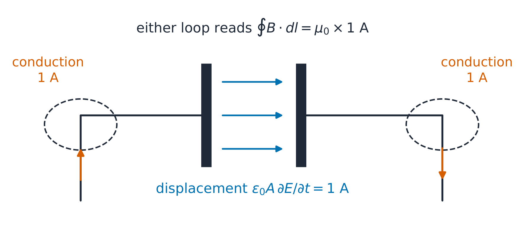
Start with the worked charging current of 1 A and compare a surface cutting the wire with one passing through the vacuum gap. The original law gives different predictions; including the changing-electric-flux term makes both totals equal. Change plate area to alter the field rate while its product with ε₀A remains the same current. Hold a nonzero stored charge to distinguish electric field from changing electric field.

7.5

คลื่นระนาบ

ทำไมถึงสำคัญ. Wi-Fi, เรดาร์, แสงอาทิตย์ และ carrier ที่ 3 GHz ของ link บนโต๊ะ ทั้งหมดเป็นคำตอบเดียวกัน: คลื่นระนาบ

แนวคิด, พร้อมภาพประกอบ. ในพื้นที่ที่ไม่มีแหล่งกำเนิด สมการคลื่นมี คำตอบที่ง่ายที่สุดคือ คลื่นระนาบ: $\mathbf{E}$, $\mathbf{B}$ และ ทิศทางการแพร่กระจาย ตั้งฉากกันเป็นแบบ mutual, ในเฟสเดียวกัน มี $B = E/c$. ความต้านทานภายใน $\eta_{0} = \sqrt{\mu_{0}/\varepsilon_{0}} = 377\ \Omega$ ของสุญญากาศกำหนดอัตราส่วนของ $E$ ต่อ $H$; เวกเตอร์พอยंटิง $\mathbf{S} = \mathbf{E} \times \mathbf{H}$ ทิศทางไปตามทิศทางการแพร่กระจายพร้อม $S = E^{2}/\eta_{0}$ (ทันที; พร้อม rms ค่าของ$E$นี่คือความหนาแน่นกำลังเฉลี่ย, ในขณะที่คลื่นไซน์ที่มีแอมพลิจูด $E_{0}$ มีค่าเฉลี่ย $E_{0}^{2}/2\eta_{0}$).

คลื่นระนาบเคลื่อนที่ตามแกน z: E และ B สั่นสะเทือนพร้อมเฟสกันและตั้งฉากกัน พร้อมแสดงความยาวคลื่น 300 เมตร — E และ B พร้อมเฟสและตั้งฉากกัน; λ = 300 เมตร ที่ 1 MHz

การพิสูจน์. สำหรับ $\mathbf{E} = E_{0}\cos(\omega t - kz)\,\hat{x}$, กฎของฟาราเดย์ $\partial B/\partial t = -\partial E/\partial z$ ความหนาแน่นกำลังจะเกิดจากอิมพีแดนซ์: $B = (k/\omega)E = E/c$. ความหนาแน่นกำลังตามมาจากอิมพิแดนซ์: $H = E/\eta_{0}$, ดังนั้น $S = E \times H = E^{2}/\eta_{0}$ — จำนวนหนึ่งต่อคลื่น

ตัวอย่างทำแล้ว 1 — อ่านตัวเลขออกมา. คลื่น 100 V/m (rms) ที่ 1 MHz: $B = 100/(3 \times 10^{8}) = 0.333\ \mu$ T; ความยาวคลื่น $\lambda = c/f = 300$ เมตร; ความหนาแน่นกำลัง $S = 100^{2}/377 = 26.5$ W/m². ตรวจสอบ เส้นทางอิมพิแดนซ์: $H = 100/377 = 0.265$ A/m, และ $E \times H = 26.5$ ✓ — ทั้งสองเส้นทางตรงกันเพราะเป็นอัตราส่วนเดียวกัน

ตัวอย่างวิธีทำ 2 — ขยายผลไปยังผิวตัวนำ. ใน ตัวนำ $e^{-\alpha z}$ มม.; $\delta = \sqrt{2/(\omega\mu\sigma)}$. ทองแดง ($\sigma = 5.8 \times 10^{7}$): ที่ 50 Hz, อธิบายว่าทำไมการป้องกันจึงทำงานได้ ทำไมกระแส RF จึงวิ่งบนพื้นผิว และทำไมเส้นสัญญาณ $\delta = \sqrt{2/(2\pi \cdot 50 \cdot 4\pi \times 10^{-7} \cdot 5.8 \times 10^{7})} = 9.3$ GHz ของสายเชื่อมต่อบนโต๊ะทดสอบต้องกว้างและชุบทอง ที่1 GHz, $\delta = 2.1\ \mu$m — บางกว่าประมาณ4500เท่าสำหรับยี่สิบ สองสิบล้านเท่า ($\delta \propto 1/\sqrt{f}$ ✓). ตัวเลขเดียวนี้ อธิบายว่าทำไม shields จึงทำงานได้, ทำไมกระแส RF ลอยอยู่บนพื้นผิว, และทำไม เส้นกราฟ 3 GHz ของลิงก์บนโต๊ะทำงานต้องการทองแดงกว้างและเรียบ: ที่ 3 GHz กระแสจะอาศัย ในชั้นบนสุด1.2 µm, ดังนั้นความหยาบของผิวและการชุบใดๆ ที่นั่นกำหนดการสูญเสีย (ทองคำ การชุบป้องกันสนิม; การนำไฟฟ้าแย่กว่าทองแดง)

ข้อผิดพลาดที่พบบ่อย. การใช้ $c$ ในไดอิเล็กทริก — ความเร็วที่นั่นคือ $1/\sqrt{\mu\varepsilon}$ (≈ 0.67c ในสายโคแอกซ์ด้านล่าง). การผสม $E/H$ (377 Ω ใน พื้นที่) ด้วย $E/B$ ($c$ — ความเร็ว ไม่ใช่อิมพีแดนซ์) และลืมว่า สนามของคลื่นเป็นเฟสเดียวกันในสื่อ LOSSLESS เท่านั้น.

สรุป. คลื่นระนาบ: $E \perp B \perp \hat{k}$, $B = E/c$, $S = E^{2}/\eta_{0}$; ตัวนำกลืนคลื่นในฐานะ $e^{-z/\delta}$ ด้วย $\delta = \sqrt{2/\omega\mu\sigma}$.

สำรวจ

Both fields reverse; energy still flows forward

$\mathbf{S}=\mathbf{E}\times\mathbf{H},\quad \langle S\rangle=E_{\rm rms}^2/\eta=E_{\rm peak}^2/(2\eta)$

Start with the worked 100 V/m RMS wave at 1 MHz. Its average power is about 26.5 W/m², while its instantaneous power at a field crest is twice that. Reinterpret the same number as a peak field and the average halves. Advance half a cycle to reverse E and H together without reversing the Poynting vector. Compare a uniform dielectric to vacuum, keeping the entered electric field specified.

คำศัพท์ ฝึกฝน

English	ไทย
plane wave	คลื่นระนาบ
intrinsic impedance	อิมพีแดนส์ภายใน
Poynting vector/ˈpɔɪntɪŋ ˈvektə/	เวกเตอร์พอยติง
skin depth	ความลึกผิว
good conductor	ตัวนำที่ดี
telegrapher equations	สมการเทเลกราฟ
characteristic impedance	อิมพีแดนส์ลักษณะเฉพาะ
bounce diagram	แผนภาพการสะท้อนกลับ
cutoff frequency/ˈkʌtɒf ˈfriːkwənsi/	ความถี่ตัด
guide wavelength	ความยาวคลื่นในแนวนำ
dipole/ˈdaɪpəʊl/	เสาอากาศไดโพล
Friis equation	สมการฟริส

7.6

สายส่งสัญญาณ

ทำไมถึงสำคัญ. สายเชื่อมต่อบนโต๊ะทำงานเชื่อมบอร์ดสองแผ่นด้วย 40 เซนติเมตรของ สายโคแอกซ์; ที่ 3 GHz นั้นเท่ากับหกความยาวคลื่น — ไม่ใช่วงจรอีกต่อไป แต่เป็น สายส่งสัญญาณ

แนวคิด พร้อมภาพประกอบ สมการเทเลกราฟ พิจารณา สายเป็นอินดักแตนซ์กระจาย $L'$ และ-capacitance $C'$ ต่อเมตร: $\partial v/\partial x = -L'\partial i/\partial t$ และ $\partial i/\partial x = -C'\partial v/\partial t$. คำตอบของพวกเขาคือแรงดัน/กระแส คลื่นที่มี $v_{p} = 1/\sqrt{L'C'}$ และอิมพิแดนซ์ลักษณะเฉพาะของสาย $Z_{0} = \sqrt{L'/C'}$.

แผนภาพการสะท้อนสำหรับขั้นบันได 12 V บนสาย 50-โอห์ม ไปยังโหลดเปิด: คลื่นเข้า 12 V/0.24 A, การสะท้อน +12 V ทำให้แรงดันเพิ่มขึ้นสองเท่าและลดกระแสให้เป็นศูนย์ที่โหลด — ลายเซ็นปลายเปิด: แรงดันเพิ่มขึ้นเป็นสองเท่า, กระแสลดลงเป็นศูนย์

การหาสมการ. หาอนุพันธ์ของสมการแรกใน $x$ และสมการที่สอง ใน $t$ และตัด $\partial^{2}i/\partial x \partial t$ ออก: สมการคลื่นสำหรับ $v$ ด้วยความเร็ว $1/\sqrt{L'C'}$. ที่โหลด $Z_{L}$, การจับคู่จะให้ สัมประสิทธิ์การสะท้อน $\Gamma = (Z_{L} - Z_{0})/(Z_{L} + Z_{0})$: สายลัด ($\Gamma = -1$) จะกลับเฟส, เปิดวงจร ($\Gamma = +1$) จะเพิ่มแรงดันสองเท่าและ ตัดกระแส — แผนภาพ bounce ติดตามทุกการสะท้อน.

ตัวอย่างฝึกหัด 1 — สายโคแอกซ์จริง. RG-316-คลาส สายโคแอกซ์กับ $L' = 250$ nH/m และ $C' = 100$ pF/m: $Z_{0} = \sqrt{250 \times 10^{-9}/100 \times 10^{-12}} = \sqrt{2500} = 50\ \Omega$ ✓ (สาย มาตรฐาน — ตัวเลขถูกเลือกมาเพื่อให้เป็นเช่นนั้น); $v_{p} = 1/\sqrt{250 \times 10^{-9} \times 100 \times 10^{-12}} = 2 \times 10^{8}$ m/s = 0.67 c. ส่วน 40 ซม. ของสายเชื่อมบนโต๊ะนี้มีความยาวหกคลื่นที่ 3 GHz ($\lambda = v_{p}/f = 6.7$ ซม.) — เพื่อยืนยันแนวคิด "เส้นนำสัญญาณ ไม่ใช่วงจร" โดยใช้ อุปกรณ์บนโต๊ะทดลอง

ตัวอย่างวิธีทำ 2 — การเปลี่ยนระดับแบบเปิด. ขับดันสาย 50 Ω ด้วย ขั้นบันได 12 V แบบปลายเปิด คลื่นตกกระทบมีค่า 12 V และ $12/50 = 0.24$ A. ที่จุดเปิด $\Gamma = +1$: ความสะท้อน +12 V จะเพิ่มขึ้นเป็นสองเท่า แรงดันโหลดจะเข้าสู่ค่า 24 V และกระแสสะท้อน $-0.24$ A จะหักล้างกัน VSWR มีแนวโน้มเป็นอนันต์ ซึ่งเป็นลายเซ็นของวงจรเปิดที่เครื่องวัดคลื่นนิ่งจะอ่านได้ เมื่อ VSWR มีแนวโน้มเป็นอนันต์ ลายเซ็นวงจรเปิดจะบ่งบอกถึงคลื่นนิ่ง ที่มิเตอร์อ่านค่าได้

ข้อผิดพลาดพบบ่อย. ใช้ $Z_{0}$ เป็นความต้านทานทางกายภาพ (ซึ่งเป็น อัตราส่วน; สาย 50 Ω ที่ไม่มีสูญเสียจะไม่กระจายพลังงาน) คำนวณ $\lambda$ ด้วย $c$ แทนที่จะใช้ $v_{p}$ (เกิดข้อผิดพลาด 30% ใน PTFE) และลืมการสะท้อนจากด้านแหล่งจ่าย: เครื่องขับที่ไม่ตรงกันจะสะท้อนกลับ และแผนภาพ bounce ต้องรวมสิ่งนี้ไว้ด้วย การสะท้อน: ตัวขับที่ไม่เข้ากันจะสะท้อนกลับ และแผนภาพการกระเจิงต้อง รวมมันไว้ด้วย

สรุป. $Z_{0} = \sqrt{L'/C'}$, $v_{p} = 1/\sqrt{L'C'}$; $\Gamma = (Z_{L}-Z_{0})/(Z_{L}+Z_{0})$; จุดเปิดเพิ่มแรงดันสองเท่า จุดลัดลดเหลือศูนย์; เส้นยาวเป็นคลื่น และแผนภาพการสะท้อนคือระบบบันทึกข้อมูล

สำรวจ

Follow the step to the load and back

$\Gamma=(R-Z_0)/(R+Z_0),\quad V=V^++V^-,\quad I=(V^+-V^-)/Z_0$

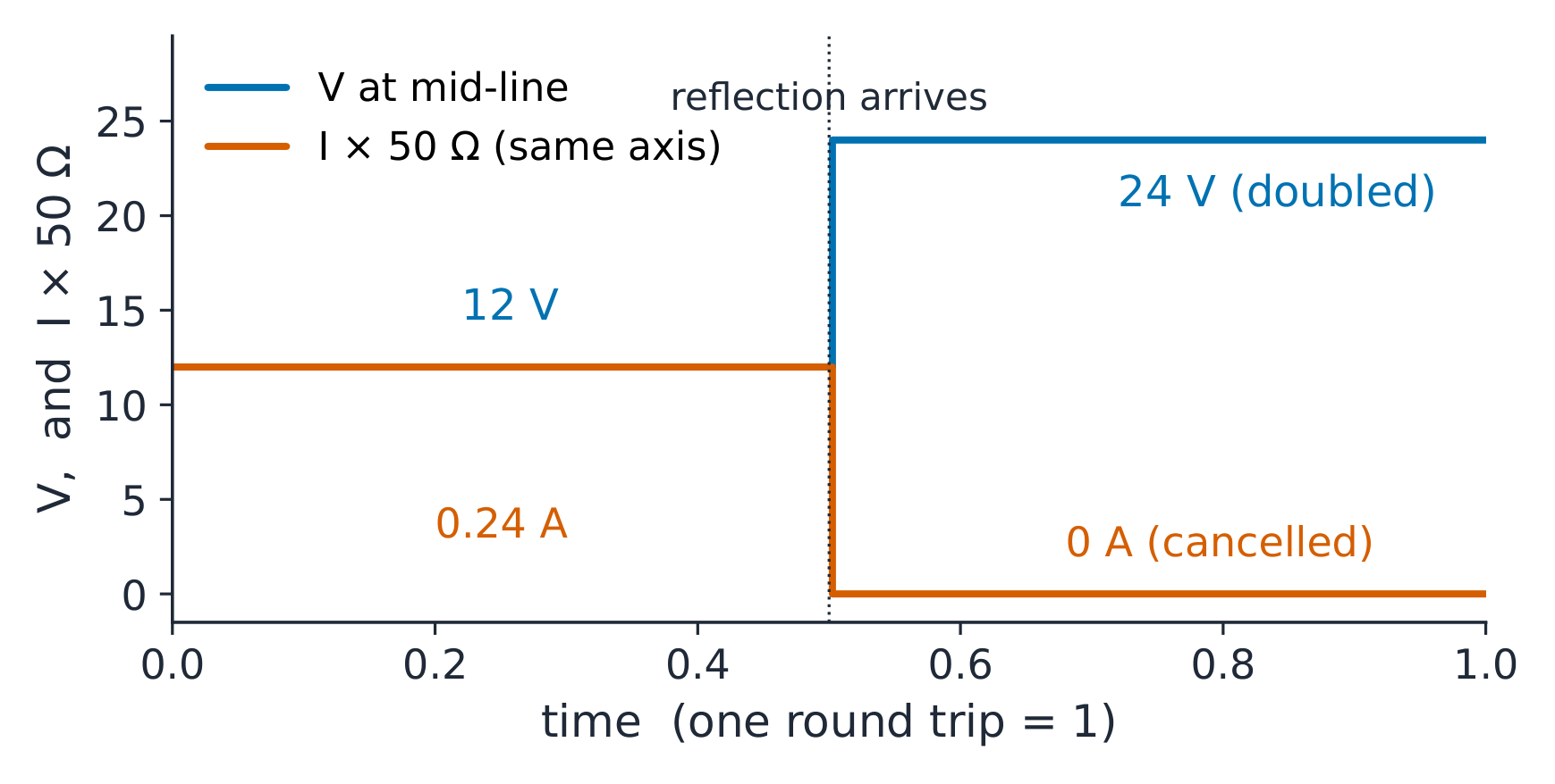
A 24 V source with 50 Ω series resistance launches the worked 12 V incident step. Follow its finite propagation delay to the open load, where voltage doubles and current cancels. Compare a short and a matched load, then change the source resistance to see whether the returning wave is absorbed or reflected again.

คำศัพท์ ฝึกฝน

English	ไทย
capacitance/kəˈpæsɪtəns/	ความจุไฟฟ้า

7.7

ท่อส่งคลื่นและเสาอากาศ

ความสำคัญ. เหนือ ~10 GHz สายโคแอกซ์จะสูญเสียพลังงานมากเกินไป; เชื่อมต่อบนโต๊ะทำงาน _backhaul (และเรดาร์ทุกชนิด) จะเปลี่ยนมาใช้ท่อกลวง และเมตรสุดท้ายของ การเชื่อมโยงวิทยุทุกชนิดคือเสาอากาศเสมอ.

แนวคิด พร้อมภาพประกอบ. ท่อโลหะกลวงนำคลื่นได้เฉพาะเมื่อมี เหนือความถี่ ตัด (cutoff): โหมดหลักของคู่อารมณ์แบบสี่เหลี่ยมผืนผ้าจะ ตัดที่ $f_{c} = c/(2a)$ ($a$ = ขนาดกว้าง) เหนือความถี่ตัดแล้ว ความยาวคลื่น ในคู่อารมณ์จะยืดออก: $\lambda_{g} = \lambda/\sqrt{1 - (f_{c}/f)^{2}}$ — คลื่นเดินทางแบบคดงอ ดังนั้นจำนวนรอบตามแกนต่อเมตรของท่อจึงน้อยลง รอบต่อเมตรของท่อ เสาอากาศปิดวงจรเชื่อมโยง: ครึ่งคลื่น ดิปอล มีกำลังขยาย 2.15 dBi และความต้านทานอินพุต ≈ 73 Ω; ค่า แต่ละ dB ในโซ่คือการตัดสินใจในการออกแบบ; พจน์สุดท้ายคือเรขาคณิตล้วนๆ

$$P_{r}/P_{t} = G_{r}G_{t}\left(\frac{\lambda}{4\pi R}\right)^{2}.$$

งบประมาณลิงค์ฟริสในลักษณะของห่วงโซ่: กำลังส่ง, กำลังขยายเสาอากาศ, ปัจจัยการกระจาย, กำลังรับ — เสาอากาศ 10-dBi สองตัว ระยะห่าง 1 กม. ที่ความถี่ 3 GHz — ทุก dB ในห่วงโซ่คือการตัดสินใจด้านการออกแบบ; พจน์สุดท้ายคือเรขาคณิตล้วนๆ

การพิสูจน์. ระหว่างแผ่นของคู่อารมณ์ สนามไฟฟ้าจะต้องปรับให้เข้ากับ คลื่นนิ่งครึ่งคลื่นตาม $a$: ที่ $a = \lambda_{c}/2$ เมื่อความถี่ตัด ดังนั้น $f_{c} = c/2a$. ตามแนวคู่อารมณ์ ค่าคงที่การแพร่กระจายจะสอดคล้องกับ $k_{g}^{2} = k^{2} - (\pi/a)^{2}$; การแก้สมการเพื่อหาค่าความยาวคลื่นจะได้สูตร การยืดออกข้างต้น ห่วงโซ่ฟริสเป็นการคูณกัน: กำลังส่ง × ทั้งคู่ ผลคูณของกำลัง × ตัวคูณการกระจาย $(\lambda/4\pi R)^{2}$ — ซึ่งเป็นอัตราส่วนพื้นที่ คือ ช่องรับสัญญาณเสาอากาศเทียบกับพื้นที่ทรงกลม

ตัวอย่างคำนวณ 1 — WR-90 ที่แถบ X เสานำคลื่น WR-90 มี $a = 22.86$ มิลลิเมตร: $f_{c} = 3 \times 10^{8}/(2 \times 0.02286) = 6.56$ กิกะเฮิร์ตซ์ — แถบ X (8.2–12.4 กิกะเฮิร์ตซ์) ทำงานเหนือค่าตัดต่อ ได้ที่ 10 กิกะเฮิร์ตซ์ ($\lambda = 30$ มิลลิเมตร): $\lambda_{g} = 30/\sqrt{1 - 0.656^{2}} = 39.8$ มิลลิเมตร — ยาวกว่าในสุญญากาศ 33% ตรวจสอบขอบเขต: เมื่อ $f \to f_{c}$, $\lambda_{g} \to \infty$ (คลื่นหยุด); เมื่อ $f \to \infty$, $\lambda_{g} \to \lambda$ (รูปแบบ zigzag หายไป) ✓

ตัวอย่างคำนวณ 2 — งบประมาณลิงก์บนโต๊ะทำงาน เสาอากาศสองตัวที่มี 10 dBi (G = 10) วางห่างกัน 1 เมตร บนโต๊ะทำงาน ที่ความถี่ 3 กิกะเฮิร์ตซ์ ($\lambda = 0.1$ เมตร): $P_{r}/P_{t} = 10 \times 10 \times (0.1/(4\pi \times 1))^{2} = 100 \times 6.33 \times 10^{-5} = 6.3 \times 10^{-3}$ — มีการสูญเสีย 22 dB ยังจัดการได้ง่ายบนโต๊ะทำงาน ขยายระยะให้แผ่นวงจรเดียวกันห่างกัน 1 กิโลเมตร: $(0.1/(4\pi \times 1000))^{2} = 6.33 \times 10^{-11}$, คูณด้วย 100 = $6.3 \times 10^{-9}$ (−82 dB) — งบประมาณลิงก์ที่ใช้กำหนดขนาดจานรับสัญญาณ หนึ่ง สูตร สองสเกล และอัตราส่วนระหว่างมันคือเรขาคณิตบริสุทธิ์ ($R^{2}$, เป็นปัจจัยของ $10^{6}$ ✓)

ข้อผิดพลาดที่พบบ่อย การใช้มิติแคบของเสานำสำหรับ $f_{c}$ (ค่าตัดต่อ ถูกกำหนดโดยมิติกว้าง) การนำไปใช้ $\lambda_{g}$ เหมือนกับ $\lambda$ ในสมการ Friis (ความยาวคลื่นในสุญญากาศควรอยู่ในตำแหน่งนั้น) และการระบุค่ากำไรของไดโพลเป็น dB โดยไม่ใส่ "i": 2.15 dBi เปรียบเทียบกับ isotropic; เปรียบเทียบกับไดโพล จะมีค่าเป็นศูนย์

สรุป. คู่มือ: $f_{c} = c/2a$, $\lambda_{g} = \lambda/\sqrt{1-(f_{c}/f)^{2}}$ (ยืดออก, เป็นอนันต์ที่จุดตัด). เสาอากาศ: ฟอร์ริส $P_{r}/P_{t} = G_{r}G_{t}(\lambda/4\pi R)^{2}$ —เรขาคณิตกำหนดพจน์สุดท้าย ทุกครั้ง

สำรวจ

A transverse half-wave decides whether the mode travels

$f_c=c/(2a),\quad \beta^2=k^2-(\pi/a)^2,\quad \lambda_g=2\pi/\beta$

Start with WR-90 at 10 GHz and compare its 39.8 mm guide wavelength with the 30 mm free-space wavelength. Change the wide dimension and frequency to cross cutoff. The transverse field still fits the walls, but the axial pattern changes from a travelling wave to a decaying field. Near cutoff, its phase spacing becomes very long.