Skip to content · ⁨ข้ามไปยังเนื้อหา⁩
Subjects · ⁨รายวิชา⁩

A-Level Further Mathematics · ⁨Further Mathematics A-Level⁩

Tips · ⁨เคล็ดลับ⁩

A-Level Further Mathematics (9231) ตั้งอยู่บนพื้นฐานของ 9709 และสมมติว่าผู้เรียนมีความรู้ในรายวิชานั้นอยู่แล้ว: Further Pure 1 และ 2, Further Mechanics และ Further Probability & Statistics วิชานี้จะเรียนไปพร้อมๆ กับ Maths ไม่ใช่แทนที่ และส่วนประกอบใดที่จะเข้าสอบขึ้นอยู่กับเกณฑ์การรับเข้าของโรงเรียนคุณ

Further Pure เป็นส่วนที่บรรจุกลไกใหม่ๆ ไว้มากที่สุด —包括 matrices และ linear transformations, numbers ในรูป polar และ exponential, curves แบบ polar, hyperbolic functions, differential equations และ proof by induction นี่คือเนื้อหาใหม่จริงๆ ไม่ใช่แค่ความยากขึ้นของเนื้อหาเดิมที่คุ้นเคย

ความยากที่แท้จริงคือ เวลา ไม่ใช่ความคิด การคำนวณทางพีชคณิตมีความยาวพอที่ ข้อผิดพลาดในบรรทัดที่สองจะติดมาจนถึงตอนจบ ดังนั้นให้เขียนวิธีทำอย่างละเอียดและตรวจสอบที่จุดกึ่งกลาง

  • 1

    Further Pure Mathematics 1 · ⁨คณิตศาสตร์บริสุทธิ์เพิ่มเติม 1⁩

    Watch lesson · ⁨ดูบทเรียน⁩
    English

    This handout covers Topic 1: Further Pure Mathematics 进阶纯数学 1. It adds new algebra, matrices, polar coordinates, more vectors, and proof by induction.

    ไทย

    เอกสารฉบับนี้ครอบคลุมหัวข้อที่ 1: คณิตศาสตร์บริสุทธิ์เพิ่มเติม 1 เพิ่มพีชคณิตใหม่ เมทริกซ์ พิกัดขั้วเวกเตอร์เพิ่มเติมและการพิสูจน์ด้วยการอุปนัย

    1.1

    Roots of polynomial equations · ⁨รากของสมการพหุนาม⁩

    Syllabus · ⁨หลักสูตร⁩
    English
    Candidates should be able to: Notes and examples
    • recall and use the relations between the roots and coefficients of polynomial equations e.g. to evaluate symmetric functions of the roots or to solve problems involving unknown coefficients in equations; restricted to equations of degree 2, 3 or 4 only.
    • use a substitution to obtain an equation whose roots are related in a simple way to those of the original equation Substitutions will not be given for the easiest cases, e.g. where the new roots are reciprocals or squares or a simple linear function of the old roots.
    ไทย
    ผู้เข้าสอบควรสามารถ: หมายเหตุและตัวอย่าง
    • จำและใช้ความสัมพันธ์ระหว่าง ราก และ สัมประสิทธิ์ ของสมการพหุนาม เช่น เพื่อคำนวณ ฟังก์ชันสมมาตร ของรากหรือแก้ปัญหาที่เกี่ยวข้องกับสัมประสิทธิ์ที่ไม่ทราบในสมการ; จำกัดเฉพาะสมการที่มีดีกรี 2, 3 หรือ 4 เท่านั้น.
    • ใช้ การแทนค่า เพื่อให้ได้สมการwhose roots are related in a simple way to those of the original equation การแทนค่าจะไม่ให้สำหรับกรณีที่ง่ายที่สุด, เช่น ที่รากใหม่เป็น reciprocals หรือกำลังสองหรือฟังก์ชันเชิงเส้นที่เรียบง่ายของรากเก่า.

    Source: Cambridge International syllabus · ⁨แหล่งที่มา: หลักสูตร Cambridge International⁩

    English

    For a polynomial equation, the roots 根 are linked to the coefficients 系数. For $ax^2 + bx + c = 0$ with roots $\alpha, \beta$:

    $$\alpha + \beta = -\frac{b}{a}, \qquad \alpha\beta = \frac{c}{a}.$$
    For a cubic $ax^3 + bx^2 + cx + d = 0$ with roots $\alpha, \beta, \gamma$:
    $$\sum\alpha = -\frac{b}{a}, \qquad \sum\alpha\beta = \frac{c}{a}, \qquad \alpha\beta\gamma = -\frac{d}{a}.$$
    Sums like $\sum\alpha$ and $\sum\alpha\beta$ are symmetric functions 对称函数 of the roots (unchanged if the roots are swapped). To find an equation whose roots are changed in a simple way, use a substitution 代换 (for example, put $w = \alpha + 1$).

    Worked example. The equation $x^2 - 5x + 6 = 0$ has roots $\alpha, \beta$. Find the equation with roots $\alpha + 1, \beta + 1$.

    Here $\alpha + \beta = 5$ and $\alpha\beta = 6$. The new sum is $(\alpha + 1) + (\beta + 1) = 7$, and the new product is $(\alpha + 1)(\beta + 1) = \alpha\beta + \alpha + \beta + 1 = 6 + 5 + 1 = 12$. So the new equation is

    $$x^2 - 7x + 12 = 0.$$

    ไทย

    สำหรับสมการพหุนาม ราก จะเชื่อมโยงกับ สัมประสิทธิ์ สำหรับ $ax^2 + bx + c = 0$ ที่มีราก $\alpha, \beta$:

    $$\alpha + \beta = -\frac{b}{a}, \qquad \alpha\beta = \frac{c}{a}.$$
    สำหรับสมการกำลังสาม $ax^3 + bx^2 + cx + d = 0$ ที่มีราก $\alpha, \beta, \gamma$:
    $$\sum\alpha = -\frac{b}{a}, \qquad \sum\alpha\beta = \frac{c}{a}, \qquad \alpha\beta\gamma = -\frac{d}{a}.$$
    ผลบวกแบบ $\sum\alpha$ และ $\sum\alpha\beta$ เป็น ฟังก์ชันสมมาตร ของราก (ไม่เปลี่ยนแปลงหากสลับราก) เพื่อหาสมการwhose roots are changed in a simple way, ใช้ การแทนค่า (เช่น วาง $w = \alpha + 1$)

    ตัวอย่างทำ. สมการ $x^2 - 5x + 6 = 0$ มีราก $\alpha, \beta$. หาสมการwhose roots are $\alpha + 1, \beta + 1$.

    ที่นี่ $\alpha + \beta = 5$ และ $\alpha\beta = 6$. ผลบวกใหม่คือ $(\alpha + 1) + (\beta + 1) = 7$ และผลคูณใหม่คือ $(\alpha + 1)(\beta + 1) = \alpha\beta + \alpha + \beta + 1 = 6 + 5 + 1 = 12$. ดังนั้นสมการใหม่คือ

    $$x^2 - 7x + 12 = 0.$$

    Explore · ⁨สำรวจ⁩

    Roots of a polynomial · ⁨รากของพหุนาม⁩

    y = ax³ + bx² + cx + d

    The roots are where the curve meets the x-axis — their sum and product link to the coefficients. · ⁨รากคือจุดที่กราฟตัดแกน x — ผลบวกและผลคูณของรากเชื่อมโยงกับสัมประสิทธิ์⁩

    Vocabulary · ⁨คำศัพท์⁩ Train · ⁨ฝึกฝน⁩
    English ไทย
    Further Pure Mathematics/ˈfɜːðə pjʊə ˌmæθɪˈmætɪks/ คณิตศาสตร์บริสุทธิ์เพิ่มเติม
    roots/ruːts/ ราก
    coefficients/ˌkəʊɪˈfɪʃənts/ สัมประสิทธิ์
    substitution/ˌsʌbstɪˈtjuːʃn/ substitution
    rational function/ˈræʃənl ˈfʌŋkʃn/ ฟังก์ชันตรรกยะ
    1.2

    Rational functions and graphs · ⁨ฟังก์ชันตรรกยะและกราฟ⁩

    Syllabus · ⁨หลักสูตร⁩
    English
    Candidates should be able to: Notes and examples
    • sketch graphs of simple rational functions, including the determination of oblique asymptotes, in cases where the degree of the numerator and the denominator are at most 2 Including determination of the set of values taken by the function, e.g. by the use of a discriminant. Detailed plotting of curves will not be required, but sketches will generally be expected to show significant features, such as turning points, asymptotes and intersections with the axes.
    • understand and use relationships between the graphs of $y = f(x)$, $y^2 = f(x)$, $y = \frac{1}{f(x)}$, $y = |f(x)|$ and $y = f(|x|)$ Including use of such sketch graphs in the course of solving equations or inequalities.
    ไทย
    ผู้เข้าสอบควรสามารถ: หมายเหตุและตัวอย่าง
    • วาดกราฟของ ฟังก์ชันตรรกยะ แบบง่าย, بما其中包括การกำหนด เส้นสัมผัสเฉียง, ในกรณีที่ดีกรีของตัวเศษและตัวส่วนไม่เกิน 2 รวมถึงการกำหนดเซตของค่าที่ฟังก์ชันรับ, เช่น通过使用 discriminant. การวาดกราฟโดยละเอียดจะไม่ต้องการ, แต่จะคาดหวังให้ภาพร่างแสดงลักษณะสำคัญ, เช่น จุดเปลี่ยน, เส้นอสมптอท และจุดตัดกับแกน.
    • เข้าใจและใช้ความสัมพันธ์ระหว่างกราฟของ $y = f(x)$, $y^2 = f(x)$, $y = \frac{1}{f(x)}$, $y = |f(x)|$ และ $y = f(|x|)$ รวมถึงการใช้กราฟภาพร่างเช่นนี้ในกระบวนการแก้สมการหรืออสมการ.

    Source: Cambridge International syllabus · ⁨แหล่งที่มา: หลักสูตร Cambridge International⁩

    English

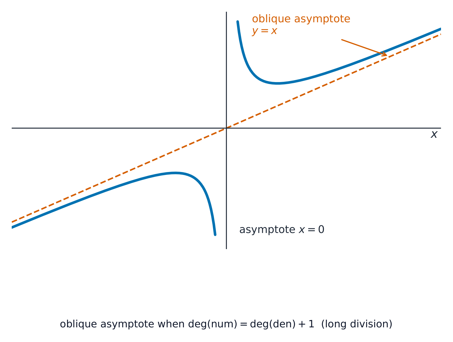
    A rational function 有理函数 is a fraction of two polynomials. When the top has degree exactly one higher than the bottom, the graph has an oblique asymptote 斜渐近线 (a slanted line the curve approaches); find it by dividing out. You should also be able to relate the graph of $y = f(x)$ to those of $y^2 = f(x)$, $y = \dfrac{1}{f(x)}$, $y = |f(x)|$ and $y = f(|x|)$. Find the set of values the function can take using the discriminant 判别式, and locate its turning points 驻点.

    Worked example. Find the oblique asymptote of $y = \dfrac{x^2 + x + 1}{x + 1}$.

    Divide out the fraction: $\dfrac{x^2 + x + 1}{x + 1} = x + \dfrac{1}{x + 1}$. As $x \to \pm\infty$ the remainder $\dfrac{1}{x+1} \to 0$, so the curve approaches the line $y = x$ — the oblique asymptote.

    ไทย

    ฟังก์ชันตรรกยะ เป็นเศษส่วนของพหุนามสองตัว เมื่อตัวบนมีดีกรีสูงกว่าตัวล่างพอดีหนึ่งขั้น กราฟจะมี เส้นเอียงอนันต์ (เส้นเฉียงที่เส้นโค้งเข้าใกล้); หาค่าได้โดยการหารออก คุณควร还能 connects the graph of $y = f(x)$ to those of $y^2 = f(x)$, $y = \dfrac{1}{f(x)}$, $y = |f(x)|$ and $y = f(|x|)$. หาเซตของค่าที่ฟังก์ชันสามารถรับได้โดยใช้ ดิสคริมิแนนต์ และระบุจุด เปลี่ยนทิศทาง ของมัน

    เส้นโค้งตรรกยะสองสาขาวิ่งคู่ไปกับเส้นประเฉียง
    ห่างจากจุดกำเนิด เส้นโค้งโอบล้อมเส้นเฉียง $y=x$; ใกล้ $x=0$ มันวิ่งออกไปตามเส้นอนันต์แนวตั้ง

    ตัวอย่างทำ. หาเส้นเอียงอนันต์ของ $y = \dfrac{x^2 + x + 1}{x + 1}$.

    หารเศษส่วนออก: $\dfrac{x^2 + x + 1}{x + 1} = x + \dfrac{1}{x + 1}$. เมื่อ $x \to \pm\infty$ เศษเหลือ $\dfrac{1}{x+1} \to 0$ ดังนั้นกราฟจะเข้าใกล้เส้น $y = x$ — ซึ่งคือเส้นอสมптอทเฉียง

    Explore · ⁨สำรวจ⁩

    Rational functions · ⁨ฟังก์ชันเศษส่วน⁩

    y = a/(x − b) + c

    A rational function has asymptotes the curve approaches but never touches. · ⁨ฟังก์ชันเศษส่วนมี เส้นประ ที่กราฟเข้าใกล้แต่ไม่เคยสัมผัส⁩

    Vocabulary · ⁨คำศัพท์⁩ Train · ⁨ฝึกฝน⁩
    English ไทย
    oblique asymptote/əˈbliːk ˈæsɪmptəʊt/ เส้นเอียงลิมิต
    method of differences/ˈmeθəd ɒv ˈdɪfrənsɪz/ วิธีผลต่าง
    convergent/kənˈvɜːdʒənt/ การชนกัน (convergent)
    sum to infinity/sʌm tʊ ɪnˈfɪnɪti/ ผลบวกถึงอนันต์
    1.3

    Summation of series · ⁨ผลรวมของอนุกรม⁩

    Syllabus · ⁨หลักสูตร⁩
    English
    Candidates should be able to: Notes and examples
    • use the standard results for $\sum r$, $\sum r^2$, $\sum r^3$ to find related sums
    • use the method of differences to obtain the sum of a finite series Use of partial fractions to express a general term in a suitable form may be required.
    • recognise, by direct consideration of a sum to $n$ terms, when a series is convergent, and find the sum to infinity in such cases
    ไทย
    ผู้เข้าสอบควรสามารถ: หมายเหตุและตัวอย่าง
    • ใช้ผลลัพธ์มาตรฐานสำหรับ $\sum r$, $\sum r^2$, $\sum r^3$ เพื่อหาผลรวมที่เกี่ยวข้อง
    • ใช้ วิธีผลต่าง เพื่อหาผลรวมของอนุกรมจำกัด การใช้ เศษส่วนย่อย เพื่อแสดงพจน์ทั่วไปในรูปแบบที่เหมาะสมอาจจำเป็น.
    • ชี้ชัดว่าเมื่อใดอนุกรมหนึ่งจะเป็น ลู่เข้า โดยพิจารณาผลบวก $n$ พจน์โดยตรง และหาค่า ผลบวกอนันต์ ในกรณีดังกล่าว

    Source: Cambridge International syllabus · ⁨แหล่งที่มา: หลักสูตร Cambridge International⁩

    English

    Learn the standard results:

    $$\sum_{r=1}^{n} r = \tfrac12 n(n+1), \qquad \sum_{r=1}^{n} r^2 = \tfrac16 n(n+1)(2n+1), \qquad \sum_{r=1}^{n} r^3 = \tfrac14 n^2(n+1)^2.$$
    The method of differences 差分法 sums a series by cancelling middle terms: if partial fractions 部分分式 write each term as $f(r) - f(r+1)$, almost everything cancels. From the sum to $n$ terms you can see whether a series is convergent 收敛 and, if so, find its sum to infinity 无穷和.

    Worked example. Find $\displaystyle\sum_{r=1}^{n} (2r + 1)$.

    $$\sum_{r=1}^{n}(2r + 1) = 2\sum_{r=1}^{n} r + \sum_{r=1}^{n} 1 = 2\cdot\tfrac12 n(n+1) + n = n(n+1) + n = n(n+2).$$

    ไทย

    เรียนรู้ผลลัพธ์มาตรฐาน:

    $$\sum_{r=1}^{n} r = \tfrac12 n(n+1), \qquad \sum_{r=1}^{n} r^2 = \tfrac16 n(n+1)(2n+1), \qquad \sum_{r=1}^{n} r^3 = \tfrac14 n^2(n+1)^2.$$
    วิธีผลต่าง รวมนิพจน์โดยตัดพจน์ตรงกลางออก: ถ้าใช้ เศษส่วนย่อย เขียนแต่ละพจน์ในรูป $f(r) - f(r+1)$, แทบทุกสิ่งจะตัดกัน จากผลรวมของ $n$ พจน์ คุณสามารถตรวจสอบว่าอนุกรมนี้เป็น อนุกรมลู่เข้า หรือไม่ และหากเป็น如此 จะหา ผลรวมอนันต์ ของมันได้

    ตัวอย่างมีคำตอบ. หา $\displaystyle\sum_{r=1}^{n} (2r + 1)$.

    $$\sum_{r=1}^{n}(2r + 1) = 2\sum_{r=1}^{n} r + \sum_{r=1}^{n} 1 = 2\cdot\tfrac12 n(n+1) + n = n(n+1) + n = n(n+2).$$

    Explore · ⁨สำรวจ⁩

    Sequences and their sums · ⁨อนุกรมและผลรวมของ它们⁩

    Step through the terms and the running total — the idea behind a series and its sum to n terms. · ⁨เดินผ่านพจน์และผลรวมสะสม — แนวคิดเรื่อง อนุกรม และผลรวมถึง n พจน์⁩

    1.4

    Matrices · ⁨เมทริกซ์⁩

    Syllabus · ⁨หลักสูตร⁩
    English
    Candidates should be able to: Notes and examples
    carry out operations of matrix addition, subtraction and multiplication, and recognise the terms zero matrix and identity (or unit) matrix Including non-square matrices. Matrices will have at most 3 rows and columns.
    recall the meaning of the terms singular and non-singular as applied to square matrices and, for $2 \times 2$ and $3 \times 3$ matrices, evaluate determinants and find inverses of non-singular matrices The notations $\det \mathbf{M}$ for the determinant of a matrix $\mathbf{M}$, and $\mathbf{I}$ for the identity matrix, will be used.
    understand and use the result, for non-singular matrices, $(\mathbf{AB})^{-1} = \mathbf{B}^{-1}\mathbf{A}^{-1}$ Extension to the product of more than two matrices may be required.
    understand the use of $2 \times 2$ matrices to represent certain geometric transformations in the $x$-$y$ plane, in particular: – understand the relationship between the transformations represented by $\mathbf{A}$ and $\mathbf{A}^{-1}$ – recognise that the matrix product $\mathbf{AB}$ represents the transformation that results from the transformation represented by $\mathbf{B}$ followed by the transformation represented by $\mathbf{A}$ – recall how the area scale factor of a transformation is related to the determinant of the corresponding matrix – find the matrix that represents a given transformation or sequence of transformations Understanding of the terms rotation, reflection, enlargement, stretch and shear for 2D transformations will be required. Other 2D transformations may be included, but no particular knowledge of them is expected.
    understand the meaning of invariant as applied to points and lines in the context of transformations represented by matrices, and solve simple problems involving invariant points and invariant lines. e.g. to locate the invariant points of the transformation represented by $\begin{pmatrix} 6 & 5 \\ 2 & 3 \end{pmatrix}$, or to find the invariant lines through the origin for $\begin{pmatrix} 4 & -1 \\ 2 & 1 \end{pmatrix}$, or to show that any line with gradient 1 is invariant for $\begin{pmatrix} 2 & 0 \\ 1 & 1 \end{pmatrix}$.
    ไทย
    ผู้เข้าสอบควรสามารถ: หมายเหตุและตัวอย่าง
    ทำการดำเนินการของ การบวกเมทริกซ์, การลบ และการคูณเมทริกซ์ และระบุคำศัพท์ เมทริกซ์ศูนย์ และ เมทริกซ์เอกลักษณ์ (หรือเมทริกซ์หน่วย) รวมถึงเมทริกซ์ที่ไม่เป็นสี่เหลี่ยม จตุรัส เมทริกซ์จะมีจำนวนแถวและหลักไม่เกิน 3
    ทบทวนความหมายของคำว่า เอกฐาน และ ไม่เอกฐาน ที่ใช้กับเมทริกซ์สี่เหลี่ยมจตุรัส และสำหรับเมทริกซ์ขนาด $2 \times 2$ และ $3 \times 3$ ให้คำนวณ ดีเทอร์มิแนนต์ และหา อินเวอร์ส ของเมทริกซ์ที่ไม่เอกฐาน จะใช้สัญลักษณ์ $\det \mathbf{M}$ สำหรับดีเทอร์มิแนนต์ของเมทริกซ์ $\mathbf{M}$ และ $\mathbf{I}$ สำหรับเมทริกซ์เอกลักษณ์
    เข้าใจและใช้ผลลัพธ์สำหรับเมทริกซ์ที่ไม่เอกฐาน: $(\mathbf{AB})^{-1} = \mathbf{B}^{-1}\mathbf{A}^{-1}$ อาจต้องการขยายไปยังผลคูณของเมทริกซ์มากกว่าสองเมทริกซ์
    เข้าใจการใช้เมทริกซ์ $2 \times 2$ เพื่อแสดงการเปลี่ยนแปลงทางเรขาคณิตบางประเภทในระนาบ $x$-$y$ โดยเฉพาะ: – เข้าใจความสัมพันธ์ระหว่างการเปลี่ยนแปลงที่แทนด้วย $\mathbf{A}$ และ $\mathbf{A}^{-1}$ – ชี้ชัดว่าผลคูณเมทริกซ์ $\mathbf{AB}$ แสดงถึงการเปลี่ยนแปลงที่เกิดจากการเปลี่ยนแปลงที่แทนด้วย $\mathbf{B}$ ตามด้วยการเปลี่ยนแปลงที่แทนด้วย $\mathbf{A}$ – ทบทวนวิธีที่ ตัวคูณพื้นที่ ของการเปลี่ยนแปลงมีความสัมพันธ์กับดีเทอร์มิแนนต์ของเมทริกซ์ที่เกี่ยวข้อง – หาเมทริกซ์ที่แสดงการเปลี่ยนแปลงที่กำหนดให้หรือลำดับของการเปลี่ยนแปลง ต้องเข้าใจคำศัพท์ การหมุน, การสะท้อน, การขยาย, การยืด และ การคดเคี้ยว สำหรับการเปลี่ยนแปลง 2 มิติ อาจมีการเปลี่ยนแปลง 2 มิติอื่นๆ แต่ไม่จำเป็นต้องมีความรู้เฉพาะเจาะจงเกี่ยวกับพวกมัน
    เข้าใจความหมายของ ค่าคงที่ ที่ใช้กับจุดและเส้นตรงในบริบทของการเปลี่ยนแปลงที่แทนด้วยเมทริกซ์ และแก้โจทย์ปัญหาพื้นฐานเกี่ยวกับ จุดคงที่ และ เส้นคงที่ เช่น: เพื่อหาจุดคงที่ของการเปลี่ยนแปลงที่แทนด้วย $\begin{pmatrix} 6 & 5 \\ 2 & 3 \end{pmatrix}$, หรือหาเส้นคงที่ผ่านจุดกำเนิดสำหรับ $\begin{pmatrix} 4 & -1 \\ 2 & 1 \end{pmatrix}$, หรือพิสูจน์ว่าเส้นตรงทุกเส้นที่มีความชัน 1 เป็นค่าคงที่สำหรับ $\begin{pmatrix} 2 & 0 \\ 1 & 1 \end{pmatrix}$

    Source: Cambridge International syllabus · ⁨แหล่งที่มา: หลักสูตร Cambridge International⁩

    English
    A matrix moves the plane

    A matrix 矩阵 is a rectangular block of numbers. Matrix addition adds entries in matching positions; you can also subtract and multiply matrices (multiplication is row $\times$ column). The zero matrix 零矩阵 has every entry $0$, and the identity matrix 单位矩阵 (or unit matrix) $I$ leaves any matrix unchanged under multiplication.

    For a $2\times 2$ matrix $A = \begin{pmatrix} a & b \\ c & d \end{pmatrix}$, the determinant 行列式 is $\det A = ad - bc$. If $\det A \neq 0$ the matrix is non-singular (otherwise it is a singular matrix 奇异矩阵), and the inverse matrix 逆矩阵 is

    $$A^{-1} = \frac{1}{ad - bc}\begin{pmatrix} d & -b \\ -c & a \end{pmatrix}.$$
    For a product, $(AB)^{-1} = B^{-1}A^{-1}$. A $2\times 2$ matrix can represent a geometric transformation 几何变换 of the plane — a rotation 旋转, reflection 反射, enlargement 放大, stretch 拉伸 or shear 切变: the determinant gives the area scale factor, and a product $AB$ means "do $B$, then $A$". Points or lines that do not move are called invariant points 不变点 and invariant lines 不变直线.

    Worked example. Find the inverse of $A = \begin{pmatrix} 3 & 1 \\ 2 & 4 \end{pmatrix}$.

    $\det A = 3\times 4 - 1\times 2 = 10$, so

    $$A^{-1} = \frac{1}{10}\begin{pmatrix} 4 & -1 \\ -2 & 3 \end{pmatrix}.$$

    ไทย
    เมทริกซ์เคลื่อนที่ระนาบ

    เมทริกซ์ คือตารางสี่เหลี่ยมผืนผ้าของตัวเลข การบวกเมทริกซ์ บวกสมาชิกในตำแหน่งที่ตรงกัน; สามารถลบและคูณเมทริกซ์ได้ (การคูณคือแถว $\times$ คูณ คอลัมน์) เมทริกซ์ศูนย์ มีสมาชิกทุกตัวเป็น $0$, และ เมทริกซ์เอกลักษณ์ (หรือ เมทริกซ์หน่วย) $I$ ทำให้เมทริกซ์ใดไม่เปลี่ยนแปลงภายใต้การคูณ

    สำหรับเมทริกซ์ขนาด $2\times 2$ $A = \begin{pmatrix} a & b \\ c & d \end{pmatrix}$, ดีเทอร์มิแนนต์ คือ $\det A = ad - bc$. ถ้า $\det A \neq 0$ เมทริกซ์นี้จะไม่ выроเจิด (non-singular) (แต่ถ้าไม่เป็นเช่นนั้นจะเป็น เมทริกซ์ выроเจิด / singular matrix), และ เมทริกซ์ผกผัน คือ

    $$A^{-1} = \frac{1}{ad - bc}\begin{pmatrix} d & -b \\ -c & a \end{pmatrix}.$$
    สำหรับผลิตภัณฑ์, $(AB)^{-1} = B^{-1}A^{-1}$. เมทริกซ์ $2\times 2$ สามารถแสดง การแปลงเรขาคณิต ของระนาบ — การหมุน, การสะท้อน, การขยายขนาด, การยืด หรือ การบิดเบี้ยว: ดีเทอร์มิแนนต์ให้ปัจจัยการปรับพื้นที่, และการคูณ $AB$ หมายถึง "ทำ $B$, แล้ว $A$" จุดหรือเส้นที่ไม่เคลื่อนที่เรียกว่า จุดคงที่ และ เส้นคงที่

     สี่เหลี่ยมจัตุรัสหน่วยและสี่เหลี่ยมด้านขนานขนาดใหญ่ที่มัน映射ไปยังภายใต้เมทริกซ์
    เมทริกซ์ส่งสี่เหลี่ยมจัตุรัสหน่วยไปสู่สี่เหลี่ยมด้านขนานที่มีพื้นที่เท่ากับดีเทอร์มิแนนต์.

    ตัวอย่างมีคำตอบ. หาผกผันของ $A = \begin{pmatrix} 3 & 1 \\ 2 & 4 \end{pmatrix}$.

    $\det A = 3\times 4 - 1\times 2 = 10$, ดังนั้น

    $$A^{-1} = \frac{1}{10}\begin{pmatrix} 4 & -1 \\ -2 & 3 \end{pmatrix}.$$

    Explore · ⁨สำรวจ⁩

    Matrices as transformations · ⁨เมทริกซ์ในฐานะการแปลง⁩

    Change the four entries and watch the unit square map to a new shape. The determinant is the area scale factor. · ⁨เปลี่ยนองค์ประกอบทั้งสี่แล้วดูว่าสี่เหลี่ยมหน่วยถูกแปลงเป็นรูปร่างใหม่ ดีเทอร์มิแนนต์ คือปัจจัยขยายพื้นที่⁩

    Vocabulary · ⁨คำศัพท์⁩ Train · ⁨ฝึกฝน⁩
    English ไทย
    matrix/ˈmeɪtrɪks/ เมทริกซ์
    zero matrix/ˈzɪərəʊ ˈmeɪtrɪks/ เมทริกซ์ศูนย์
    identity matrix/aɪˈdentɪti ˈmeɪtrɪks/ เมทริกซ์เอกลักษณ์
    determinant/dɪˈtɜːmɪnənt/ ดีเทอร์มิแนนต์
    singular matrix/ˈsɪŋɡjʊlə ˈmeɪtrɪks/ เมทริกซ์เอกฐาน
    inverse matrix/ɪnˈvɜːs ˈmeɪtrɪks/ เมทริกซ์ผกผัน
    geometric transformation/ˌdʒiːəʊˈmetrɪk trænsfɔːˈmeɪʃn/ การแปลงเรขาคณิต
    invariant points/ɪnˈveərɪənt pɔɪnts/ จุดคงที่
    invariant lines/ɪnˈveərɪənt laɪnz/ เส้นคงที่
    polar coordinates/ˈpəʊlə kəʊˈɔːdɪnəts/ พิกัดขั้ว
    Cartesian coordinates/kɑːˈtiːzɪən kəʊˈɔːdɪnəts/ พิกัดคาร์ทีเซียน
    polar curves/ˈpəʊlə kɜːvz/ เส้นโค้งขั้ว
    Watch lesson · ⁨ดูบทเรียน⁩
    1.5

    Polar coordinates · ⁨พิกัดเชิงขั้ว⁩

    Syllabus · ⁨หลักสูตร⁩
    English
    Candidates should be able to: Notes and examples
    understand the relations between Cartesian and polar coordinates, and convert equations of curves from Cartesian to polar form and vice versa The convention $r \geqslant 0$ will be used.
    sketch simple polar curves, for $0 \leqslant \theta < 2\pi$ or $-\pi < \theta \leqslant \pi$ or a subset of either of these intervals Detailed plotting of curves will not be required, but sketches will generally be expected to show significant features, such as symmetry, coordinates of intersections with the initial line, the form of the curve at the pole and least/greatest values of $r$.
    recall the formula $\frac{1}{2} \int r^2 \mathrm{d}\theta$ for the area of a sector, and use this formula in simple cases.
    ไทย
    ผู้เข้าสอบควรสามารถ: หมายเหตุและตัวอย่าง
    เข้าใจความสัมพันธ์ระหว่าง พิกัดเดकारต และ พิกัดขั้ว และแปลงสมการของเส้นโค้งจากรูปแบบเดคารตเป็นรูปแบบขั้วและในทางกลับกัน ใช้ธรรมเนียม $r \geqslant 0$
    วาดแผนภาพ เส้นโค้งขั้ว แบบง่าย สำหรับ $0 \leqslant \theta < 2\pi$ หรือ $-\pi < \theta \leqslant \pi$ หรือช่วงย่อยของช่วงเหล่านี้ ไม่จำเป็นต้องวาดกราฟเส้นโค้งอย่างละเอียด แต่แผนภาพควรแสดงลักษณะสำคัญโดยทั่วไป เช่น ความสมมาตร, พิกัดของจุดตัดกับเส้นเริ่มต้น, รูปแบบของเส้นโค้งที่จุดกำเนิด และค่าต่ำสุด/สูงสุดของ $r$
    ทบทวนสูตร $\frac{1}{2} \int r^2 \mathrm{d}\theta$ สำหรับพื้นที่ของส่วนวงกลม และใช้สูตรนี้ในกรณีพื้นฐาน

    Source: Cambridge International syllabus · ⁨แหล่งที่มา: หลักสูตร Cambridge International⁩

    English
    Tracing a polar curve: the cardioid

    Polar coordinates 极坐标 give a point by its distance $r$ from the origin and its angle $\theta$. They link to Cartesian coordinates 直角坐标 by

    $$x = r\cos\theta, \qquad y = r\sin\theta, \qquad r^2 = x^2 + y^2.$$

    You should sketch simple polar curves 极坐标曲线, and find the area of a sector with

    $$\text{area} = \tfrac12\int r^2\,d\theta.$$

    Worked example. Convert the polar equation $r = 4\cos\theta$ to Cartesian form.

    Multiply both sides by $r$: $r^2 = 4r\cos\theta$, so $x^2 + y^2 = 4x$. Completing the square gives $(x - 2)^2 + y^2 = 4$, a circle of radius $2$ centred at $(2, 0)$.

    ไทย
    การวาดเส้นโค้งเชิงขั้ว: คาร์ดิอยด์
     มองลงบันไดเกลียวขนาดใหญ่
    บันไดเกลียว: เกลียวถูกอธิบายอย่างเป็นธรรมชาติโดยใช้พิกัดเชิงขั้ว.

    พิกัดเชิงขั้ว กำหนดจุดโดยระยะ $r$ จากจุดกำเนิดและมุม $\theta$.它们เชื่อมโยงกับ พิกัดคาร์ทีเซียน ผ่าน

    $$x = r\cos\theta, \qquad y = r\sin\theta, \qquad r^2 = x^2 + y^2.$$

     จุดที่เข้าถึงได้ด้วยระยะ r ที่มุม theta, พร้อมองค์ประกอบ x และ y ของมัน
    พิกัดเชิงขั้ว $(r,\theta)$ แปลงเป็นพิกัดคาร์ทีเซียนโดย $x=r\cos\theta$ และ $y=r\sin\theta$.

    คุณควรวาดแผนภาพ เส้นโค้งเชิงขั้ว ง่ายๆ, และหาพื้นที่ของส่วนวงกลมด้วย

    $$\text{area} = \tfrac12\int r^2\,d\theta.$$

     คาร์ดิอยด์รูปหัวใจวาดบนตารางพิกัดเชิงขั้ว
    คาร์ดิอยด์ $r=1+\cos\theta$, วาดโดยตรงจาก $r$ ในฐานะฟังก์ชันของ $\theta$

    ตัวอย่างมีคำตอบ. แปลงสมการเชิงขั้ว $r = 4\cos\theta$ เป็นรูปแบบคาร์ทีเซียน.

    คูณทั้งสองข้างด้วย $r$: $r^2 = 4r\cos\theta$, ดังนั้น $x^2 + y^2 = 4x$. การทำให้เป็นกำลังสองสมบูรณ์จะได้ $(x - 2)^2 + y^2 = 4$, ซึ่งเป็นวงกลมที่มีรัศมี $2$ และมีศูนย์กลางอยู่ที่ $(2, 0)$.

    Explore · ⁨สำรวจ⁩

    Polar curves · ⁨เส้นโค้งเชิงขั้ว⁩

    Pick a curve and change a. In polar form a point is set by its distance r and angle θ — that draws roses, cardioids and spirals. · ⁨เลือกเส้นโค้งและเปลี่ยนค่า a ในรูปแบบเชิงขั้ว จุดกำหนดโดยระยะ r และมุม θ ซึ่งสร้างรูปกุหลาบ คาร์ดิอยด์ และสไปรัล⁩

    Watch lesson · ⁨ดูบทเรียน⁩
    1.6

    Vectors · ⁨เวกเตอร์⁩

    Syllabus · ⁨หลักสูตร⁩
    English
    Candidates should be able to: Notes and examples
    use the equation of a plane in any of the forms $ax + by + cz = d$ or $\mathbf{r.n} = p$ or $\mathbf{r} = \mathbf{a} + \lambda\mathbf{b} + \mu\mathbf{c}$ and convert equations of planes from one form to another as necessary in solving problems
    recall that the vector product $\mathbf{a} \times \mathbf{b}$ of two vectors can be expressed either as $|\mathbf{a}||\mathbf{b}|\sin\theta\hat{\mathbf{n}}$, where $\hat{\mathbf{n}}$ is a unit vector, or in component form as $(a_2b_3 - a_3b_2)\mathbf{i} + (a_3b_1 - a_1b_3)\mathbf{j} + (a_1b_2 - a_2b_1)\mathbf{k}$
    use equations of lines and planes, together with scalar and vector products where appropriate, to solve problems concerning distances, angles and intersections, including: – determining whether a line lies in a plane, is parallel to a plane or intersects a plane, and finding the point of intersection of a line and a plane when it exists – finding the foot of the perpendicular from a point to a plane – finding the angle between a line and a plane, and the angle between two planes – finding an equation for the line of intersection of two planes – calculating the shortest distance between two skew lines – finding an equation for the common perpendicular to two skew lines.
    ไทย
    ผู้เข้าสอบควรสามารถ: หมายเหตุและตัวอย่าง
    ใช้สมการของ ระนาบ ในรูปแบบใดๆ คือ $ax + by + cz = d$ หรือ $\mathbf{r.n} = p$ หรือ $\mathbf{r} = \mathbf{a} + \lambda\mathbf{b} + \mu\mathbf{c}$ และแปลงสมการระนาบจากรูปแบบหนึ่งไปเป็นอีก dạngหนึ่งตามจำเป็นในการแก้ปัญหา
    ทบทวนว่า ผลคูณเวกเตอร์ $\mathbf{a} \times \mathbf{b}$ ของเวกเตอร์สองตัวสามารถเขียนได้ทั้งในรูป $|\mathbf{a}||\mathbf{b}|\sin\theta\hat{\mathbf{n}}$, ซึ่ง $\hat{\mathbf{n}}$ เป็นเวกเตอร์หน่วย, หรือในรูปแบบองค์ประกอบคือ $(a_2b_3 - a_3b_2)\mathbf{i} + (a_3b_1 - a_1b_3)\mathbf{j} + (a_1b_2 - a_2b_1)\mathbf{k}$
    ใช้สมการของเส้นตรงและระนาบ ร่วมกับ ผลคูณสเกลาร์และผลคูณเวกเตอร์ เมื่อเหมาะสม เพื่อแก้โจทย์ปัญหาเกี่ยวกับระยะห่าง มุม และจุดตัด รวมถึง: – การตรวจสอบว่าเส้นตรงอยู่ในระนาบ, ขนานกับระนาบ หรือตัดกับระนาบ และหาจุดตัดของเส้นตรงกับระนาบเมื่อมีอยู่ – การหาจุดตกตั้งฉากจากจุดหนึ่งไปยังระนาบ – การหามุมระหว่างเส้นตรงกับระนาบ และมุมระหว่างระนาบสองระนาบ – การหาสมการของเส้นตรงที่เป็นรอยตัดของระนาบสองระนาบ – การคำนวณระยะสั้นที่สุดระหว่าง เส้นตรงอ้อม – การหาสมการของเส้นตรงตั้งฉากร่วมของเส้นตรงอ้อมสองเส้น

    Source: Cambridge International syllabus · ⁨แหล่งที่มา: หลักสูตร Cambridge International⁩

    English

    In three dimensions a plane 平面 can be written as $ax + by + cz = d$, or $\mathbf{r}\cdot\mathbf{n} = p$, or $\mathbf{r} = \mathbf{a} + \lambda\mathbf{b} + \mu\mathbf{c}$. Besides the scalar product, there is the vector product 向量积 of two vectors 向量:

    $$\mathbf{a}\times\mathbf{b} = |\mathbf{a}|\,|\mathbf{b}|\sin\theta\;\hat{\mathbf{n}},$$
    which gives a vector at right angles to both. With scalar and vector products you can find distances, angles, and where lines and planes meet — including the shortest distance between skew lines 异面直线.

    Worked example. Find $\mathbf{a}\times\mathbf{b}$ for $\mathbf{a} = \mathbf{i} + \mathbf{j}$ and $\mathbf{b} = \mathbf{j} + \mathbf{k}$.

    $$\mathbf{a}\times\mathbf{b} = \begin{vmatrix} \mathbf{i} & \mathbf{j} & \mathbf{k} \\ 1 & 1 & 0 \\ 0 & 1 & 1 \end{vmatrix} = \mathbf{i}(1) - \mathbf{j}(1) + \mathbf{k}(1) = \mathbf{i} - \mathbf{j} + \mathbf{k}.$$

    ไทย
     เรือใบพร้อม sail full spinnaker
    แรงเช่นลมและน้ำคือเวกเตอร์ — พวกมันมีทั้งขนาดและทิศทาง.

    ในสามมิติ ระนาบ สามารถเขียนได้เป็น $ax + by + cz = d$, หรือ $\mathbf{r}\cdot\mathbf{n} = p$, หรือ $\mathbf{r} = \mathbf{a} + \lambda\mathbf{b} + \mu\mathbf{c}$ นอกเหนือจากผลคูณสเกลาร์แล้ว ยังมี ผลคูณเวกเตอร์ ของ เวกเตอร์ สองตัว:

    $$\mathbf{a}\times\mathbf{b} = |\mathbf{a}|\,|\mathbf{b}|\sin\theta\;\hat{\mathbf{n}},$$
    ซึ่งให้เวกเตอร์ที่ตั้งฉากกับทั้งสอง ตัว Using scalar and vector products you can find distances, angles, and where lines and planes meet — including the shortest distance between skew lines.

     Two vectors spanning a parallelogram with their vector product standing straight up
    $\mathbf{a}\times\mathbf{b}$ ตั้งฉากกับเวกเตอร์ทั้งสอง; ความยาวของมันเท่ากับพื้นที่ของสี่เหลี่ยมด้านขนานที่พวกมันสร้าง.

    ตัวอย่างมีคำตอบ. หา $\mathbf{a}\times\mathbf{b}$ สำหรับ $\mathbf{a} = \mathbf{i} + \mathbf{j}$ และ $\mathbf{b} = \mathbf{j} + \mathbf{k}$.

    $$\mathbf{a}\times\mathbf{b} = \begin{vmatrix} \mathbf{i} & \mathbf{j} & \mathbf{k} \\ 1 & 1 & 0 \\ 0 & 1 & 1 \end{vmatrix} = \mathbf{i}(1) - \mathbf{j}(1) + \mathbf{k}(1) = \mathbf{i} - \mathbf{j} + \mathbf{k}.$$

    Explore · ⁨สำรวจ⁩

    Vectors · ⁨เวกเตอร์⁩

    a · b = |a||b|cos θ

    The dot product is zero exactly when two vectors are perpendicular. · ⁨ผลคูณสเกลาร์ เป็นศูนย์ก็ต่อเมื่อเวกเตอร์สองตัว ตั้งฉากกัน⁩

    Vocabulary · ⁨คำศัพท์⁩ Train · ⁨ฝึกฝน⁩
    English ไทย
    plane/pleɪn/ ระนาบ
    vector product/ˈvektə ˈprɒdʌkt/ ผลคูณเวกเตอร์
    vectors/ˈvektəz/ เวกเตอร์
    skew lines/skjuː laɪnz/ เส้นตรงไม่ตัดกัน
    mathematical induction/ˌmæθɪˈmætɪkl ɪnˈdʌkʃn/ การพิสูจน์ด้วยอุปนัย
    conjecture/kənˈdʒektʃə/ ข้อสันนิษฐาน
    inductive proof/ɪnˈdʌktɪv pruːf/ การพิสูจน์แบบอุปนัย
    symmetric functions/sɪˈmetrɪk ˈfʌŋkʃnz/ ฟังก์ชันสมมาตร
    discriminant/dɪˈskrɪmɪnənt/ discriminant
    turning points/ˈtɜːnɪŋ pɔɪnts/ จุดกลับตัว
    partial fractions/ˈpɑːʃl ˈfrækʃnz/ การแยกเศษส่วนย่อย
    rotation/rəʊˈteɪʃn/ 旋转
    reflection/rɪˈflekʃn/ สะท้อน
    enlargement/enˈlɑːdʒmənt/ การขยาย
    stretch/stretʃ/ การขยาย
    shear/ʃɪə/ การเฉือน
    Watch lesson · ⁨ดูบทเรียน⁩
    1.7

    Proof by induction · ⁨การพิสูจน์โดยการอุปนัย⁩

    Syllabus · ⁨หลักสูตร⁩
    English
    Candidates should be able to: Notes and examples
    use the method of mathematical induction to establish a given result e.g. $\sum_{r=1}^{n} r^4 = \frac{1}{4}n^2(n+1)^2$, $u_n = \frac{1}{2}(1 + 3^{n-1})$ for the sequence given by $u_{n+1} = 3u_n - 1$ and $u_1 = 1$, $\begin{pmatrix} 4 & -1 \\ 6 & -1 \end{pmatrix}^n = \begin{pmatrix} 3 \times 2^n - 2 & 1 - 2^n \\ 3 \times 2^{n+1} - 6 & 3 - 2^{n+1} \end{pmatrix}$, $3^{2n} + 2 \times 5^n - 3$ is divisible by 8.
    recognise situations where conjecture based on a limited trial followed by inductive proof is a useful strategy, and carry this out in simple cases. e.g. find the $n$th derivative of $x e^x$, find $\sum_{r=1}^{n} r \times r!$.
    ไทย
    ผู้เข้าสอบควรสามารถ: หมายเหตุและตัวอย่าง
    ใช้วิธีการ อุปนัยทางคณิตศาสตร์ เพื่อยืนยันผลลัพธ์ที่กำหนดให้ เช่น: $\sum_{r=1}^{n} r^4 = \frac{1}{4}n^2(n+1)^2$, $u_n = \frac{1}{2}(1 + 3^{n-1})$ สำหรับลำดับที่กำหนดโดย $u_{n+1} = 3u_n - 1$ และ $u_1 = 1$, $\begin{pmatrix} 4 & -1 \\ 6 & -1 \end{pmatrix}^n = \begin{pmatrix} 3 \times 2^n - 2 & 1 - 2^n \\ 3 \times 2^{n+1} - 6 & 3 - 2^{n+1} \end{pmatrix}$, $3^{2n} + 2 \times 5^n - 3$ หารด้วย 8 ลงตัว
    ชี้ชัดสถานการณ์ที่ การคาดเดา จากตัวอย่างจำกัดตามด้วยการ พิสูจน์ด้วยการอุปนัย เป็นกลยุทธ์ที่มีประโยชน์ และดำเนินการ这在ในกรณีพื้นฐาน เช่น: หาอนุพันธ์อันดับ $n$ ของ $x e^x$, หา $\sum_{r=1}^{n} r \times r!$

    Source: Cambridge International syllabus · ⁨แหล่งที่มา: หลักสูตร Cambridge International⁩

    English
    Induction: the domino proof

    Mathematical induction 数学归纳法 proves a result for every positive integer $n$ in two steps:

    1. Base case: show the result is true for $n = 1$.
    2. Inductive step: assume it is true for $n = k$, then prove it for $n = k + 1$.

    If both steps work, the result is true for all $n$. Often you first make a conjecture 猜想 (a sensible guess) from a few cases, then confirm it by inductive proof 归纳证明.

    Worked example. Prove that $\displaystyle\sum_{r=1}^{n} r = \tfrac12 n(n+1)$.

    Base case $n = 1$: the left side is $1$ and the right side is $\tfrac12(1)(2) = 1$. True. Inductive step: assume $\displaystyle\sum_{r=1}^{k} r = \tfrac12 k(k+1)$. Then

    $$\sum_{r=1}^{k+1} r = \tfrac12 k(k+1) + (k+1) = (k+1)\left(\tfrac{k}{2} + 1\right) = \tfrac12 (k+1)(k+2).$$
    This is the formula with $n = k + 1$, so by induction it holds for all $n$.

    ไทย
    Induction: the domino proof

    การพิสูจน์โดยอุปมากรรมทางคณิตศาสตร์ ใช้ยืนยันผลลัพธ์สำหรับจำนวนเต็มบวกทุก $n$ ในสองขั้นตอน:

    1. กรณีฐาน: แสดงให้เห็นว่าผลลัพธ์นั้นเป็นจริงสำหรับ $n = 1$.
    2. ขั้นอุปนัย: สมมติว่าเป็นจริงสำหรับ $n = k$, จากนั้นพิสูจน์它为 $n = k + 1$.

    หากทั้งสองขั้นทำงานได้สำเร็จ, ผลลัพธ์จะเป็นจริงสำหรับทุก $n$. มักจะเริ่มจากการทำ ข้อสันนิษฐาน (การเดาอย่างมีเหตุผล) จากบางกรณี, แล้วยืนยันโดย การพิสูจน์แบบอุปนัย.

     A row of dominoes: the first is falling (the base case), and arrows show each one knocking over the next (the inductive step), so all of them fall
    Induction resembles dominoes: the base case toppling the first, and the inductive step making each one knock over the next — so the result holds for every n

    ตัวอย่างแบบฝึกหัด. พิสูจน์ว่า $\displaystyle\sum_{r=1}^{n} r = \tfrac12 n(n+1)$.

    กรณีฐาน $n = 1$: ด้านซ้ายคือ $1$ และด้านขวาคือ $\tfrac12(1)(2) = 1$. เป็นจริง. ขั้นอุปนัย: สมมติ $\displaystyle\sum_{r=1}^{k} r = \tfrac12 k(k+1)$. ดังนั้น

    $$\sum_{r=1}^{k+1} r = \tfrac12 k(k+1) + (k+1) = (k+1)\left(\tfrac{k}{2} + 1\right) = \tfrac12 (k+1)(k+2).$$
    นี่คือสูตรที่มี $n = k + 1$, ดังนั้นโดยการอุปนัย มันจึงเป็นจริงสำหรับทุก $n$.

    Explore · ⁨สำรวจ⁩

    Proof by induction route · ⁨เส้นทางของการพิสูจน์โดยการเหนี่ยวนำ⁩

    See induction as a first domino plus a rule that pushes every next case. · ⁨มองการเหนี่ยวนำเหมือนโดมิโนตัวแรกบวกกฎที่ดันกรณีถัดไปทุกครั้ง⁩

    Watch lesson · ⁨ดูบทเรียน⁩
    1.7

    Exam tips · ⁨ข้อแนะนำสำหรับการสอบ⁩

    English
    • Use the relationships between roots and coefficients (sum, sum of pairs, product) instead of solving the polynomial.
    • For proof by induction, set out the base case, assume the result for $n = k$, prove it for $n = k+1$, and write a clear closing statement.
    • Sketch rational-function graphs with their asymptotes and turning points; use the method of differences for a summation.
    • For matrices, know the determinant, inverse and invariant lines, and interpret each transformation geometrically.
    ไทย
    • ใช้ ความสัมพันธ์ระหว่างรากและสัมประสิทธิ์ (ผลรวม, ผลรวมของคู่, ผลคูณ) แทนการแก้พหุนาม.
    • สำหรับ การพิสูจน์ด้วยการอุปนัย, จัดการกรณีฐาน, สมมติผลลัพธ์สำหรับ $n = k$, พิสูจน์它为 $n = k+1$, และเขียนบทสรุปที่ชัดเจน.
    • วาดแผนภาพ กราฟฟังก์ชันอัตราส่วน พร้อมเส้นประสมและจุดกลับตัว; ใช้ วิธีผลต่าง สำหรับการหาผลรวม.
    • สำหรับ เมทริกซ์, ต้องรู้ดีเทอร์มิแนนต์, ผกผัน, และเส้นคงที่, และตีความการแปลงแต่ละชนิดในเชิงเรขาคณิต.
  • 2

    Further Pure Mathematics 2 · ⁨คณิตศาสตร์บริสุทธิ์เพิ่มเติม 2⁩

    Watch lesson · ⁨ดูบทเรียน⁩
    English

    This handout covers Topic 2: Further Pure Mathematics 进阶纯数学 2. It adds hyperbolic functions, eigenvalues, new differentiation and integration, de Moivre's theorem, and methods for differential equations.

    ไทย

    เอกสารฉบับนี้ครอบคลุมหัวข้อที่ 2: คณิตศาสตร์บริสุทธิ์เพิ่มเติม 2. ซึ่งเพิ่มฟังก์ชันไฮเปอร์โบลิก, ค่าเฉพาะ, การหาอนุพันธ์และการอินทิเกรตใหม่, ทฤษฎีบทเด มัวร์, และวิธีการสำหรับสมการเชิงอนุพันธ์.

    2.1

    Hyperbolic functions · ⁨ฟังก์ชันไฮเปอร์โบลิก⁩

    Syllabus · ⁨หลักสูตร⁩
    English
    Candidates should be able to: Notes and examples
    understand the definitions of the hyperbolic functions $\sinh x$, $\cosh x$, $\tanh x$, $\text{sech } x$, $\text{cosech } x$, $\text{coth } x$ in terms of the exponential function
    sketch the graphs of hyperbolic functions
    prove and use identities involving hyperbolic functions e.g. $\cosh^2 x - \sinh^2 x \equiv 1$, $\sinh 2x \equiv 2 \sinh x \cosh x$, and similar results corresponding to the standard trigonometric identities.
    understand and use the definitions of the inverse hyperbolic functions and derive and use the logarithmic forms
    ไทย
    ผู้เข้าสอบควรสามารถ: หมายเหตุและตัวอย่าง
    เข้าใจนิยามของ ฟังก์ชันไฮเปอร์โบลิก $\sinh x$, $\cosh x$, $\tanh x$, $\text{sech } x$, $\text{cosech } x$, $\text{coth } x$ ในtermsของฟังก์ชันเอ็กซ์โพเนนเชียล
    วาดกราฟของ ฟังก์ชันไฮเปอร์โบลิก
    พิสูจน์และใช้เอกลักษณ์ที่เกี่ยวข้องกับ ฟังก์ชันไฮเปอร์โบลิก เช่น: $\cosh^2 x - \sinh^2 x \equiv 1$, $\sinh 2x \equiv 2 \sinh x \cosh x$, และผลลัพธ์คล้ายคลึงกันที่สอดคล้องกับเอกลักษณ์ตรีโกณมิติมาตรฐาน
    เข้าใจและใช้นิยามของ ฟังก์ชันไฮเปอร์โบลิกผกผัน และหาและใช้รูปแบบลอการิทึม

    Source: Cambridge International syllabus · ⁨แหล่งที่มา: หลักสูตร Cambridge International⁩

    English
    cosh and sinh built from exponentials

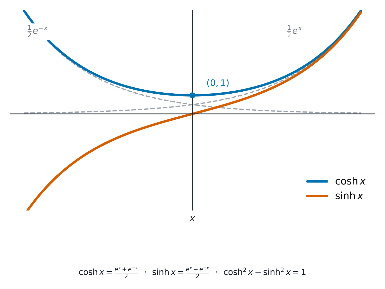
    The hyperbolic functions 双曲函数 are built from the exponential function:

    $$\cosh x = \frac{e^x + e^{-x}}{2}, \qquad \sinh x = \frac{e^x - e^{-x}}{2}, \qquad \tanh x = \frac{\sinh x}{\cosh x}.$$

    They obey identities much like the trigonometric ones, the main one being $\cosh^2 x - \sinh^2 x = 1$. The three reciprocals complete the set: $\operatorname{sech} x = \dfrac{1}{\cosh x}$, $\operatorname{cosech} x = \dfrac{1}{\sinh x}$, and $\coth x = \dfrac{1}{\tanh x} = \dfrac{\cosh x}{\sinh x}$ – all built from $e^x$ too, and worth recognising in integrals and mark schemes. The inverse hyperbolic functions 反双曲函数 have a logarithmic form 对数形式, for example $\sinh^{-1} x = \ln\!\left(x + \sqrt{x^2 + 1}\right)$.

    Worked example. Show that $\cosh^2 x - \sinh^2 x = 1$.

    $$\cosh^2 x - \sinh^2 x = \frac{(e^x + e^{-x})^2 - (e^x - e^{-x})^2}{4} = \frac{(e^{2x} + 2 + e^{-2x}) - (e^{2x} - 2 + e^{-2x})}{4} = \frac{4}{4} = 1.$$

    ไทย
    cosh และ sinh สร้างจากฟังก์ชันเอ็กซ์โพเนนเชียล
    สายเคเบิล overhead ที่ห้อยตัวเป็นเส้นโค้งระหว่างจุดรองรับ
    สายที่พาดลงจะเกิดรูปทรง catenary — ซึ่งเป็นโค้งของ hyperbolic cosine

    ฟังก์ชันไฮเปอร์โบลิกถูกสร้างจากฟังก์ชันเอ็กซ์โพเนนเชียล:

    $$\cosh x = \frac{e^x + e^{-x}}{2}, \qquad \sinh x = \frac{e^x - e^{-x}}{2}, \qquad \tanh x = \frac{\sinh x}{\cosh x}.$$

    curve cosh และ sinh พร้อมเลขชี้กำลังทั้งสองที่สร้างมันขึ้นมา
    $\cosh$ เป็นค่าเฉลี่ยของ $e^x$ และ $e^{-x}$; $\sinh$ เป็นครึ่งหนึ่งของผลต่างของทั้งสอง.

    ฟังก์ชันเหล่านี้เป็นไปตามเอกลักษณ์คล้ายกับตรีโกณมิติ โดยหลักๆ คือ $\cosh^2 x - \sinh^2 x = 1$. ฟังก์ชัน ผกผัน (reciprocals) ทั้งสามเสริมชุดนี้ให้สมบูรณ์: $\operatorname{sech} x = \dfrac{1}{\cosh x}$, $\operatorname{cosech} x = \dfrac{1}{\sinh x}$, และ $\coth x = \dfrac{1}{\tanh x} = \dfrac{\cosh x}{\sinh x}$ – ซึ่งทั้งหมดสร้างจาก $e^x$ เช่นกัน และมีประโยชน์ในการจดจำเพื่อใช้ในอินทิกรัลและสเกลคะแนน The inverse hyperbolic functions มี รูปแบบลอการิทึม, ตัวอย่างเช่น $\sinh^{-1} x = \ln\!\left(x + \sqrt{x^2 + 1}\right)$.

    ตัวอย่างวิธีทำ. แสดงว่า $\cosh^2 x - \sinh^2 x = 1$

    $$\cosh^2 x - \sinh^2 x = \frac{(e^x + e^{-x})^2 - (e^x - e^{-x})^2}{4} = \frac{(e^{2x} + 2 + e^{-2x}) - (e^{2x} - 2 + e^{-2x})}{4} = \frac{4}{4} = 1.$$

    Explore · ⁨สำรวจ⁩

    Hyperbolic functions · ⁨ฟังก์ชันไฮเปอร์โบลิก⁩

    y = a cosh(x)

    cosh is the catenary (a hanging chain) — even, with its minimum at (0, a). · ⁨cosh คือ เส้นโค้งสายโซ่ (catenary) — แม้จะมีค่าต่ำสุดที่จุด (0, a)⁩

    Vocabulary · ⁨คำศัพท์⁩ Train · ⁨ฝึกฝน⁩
    English ไทย
    Further Pure Mathematics/ˈfɜːðə pjʊə ˌmæθɪˈmætɪks/ คณิตศาสตร์บริสุทธิ์เพิ่มเติม
    hyperbolic functions/ˌhaɪpəˈbɒlɪk ˈfʌŋkʃnz/ ฟังก์ชันไฮเปอร์โบลิก
    inverse hyperbolic functions/ɪnˈvɜːs ˌhaɪpəˈbɒlɪk ˈfʌŋkʃnz/ ฟังก์ชันไฮเปอร์โบลิกผกผัน
    logarithmic form/ˌlɒɡəˈrɪθmɪk fɔːm/ รูปเลขยกกำลัง
    matrix equation/ˈmeɪtrɪks ɪˈkweɪʒn/ สมการเมทริกซ์
    2.2

    Matrices · ⁨เมทริกซ์⁩

    Syllabus · ⁨หลักสูตร⁩
    English
    Candidates should be able to: Notes and examples
    formulate a problem involving the solution of 3 linear simultaneous equations in 3 unknowns as a problem involving the solution of a matrix equation, or vice versa
    understand the cases that may arise concerning the consistency or inconsistency of 3 linear simultaneous equations, relate them to the singularity or otherwise of the corresponding matrix, solve consistent systems, and interpret geometrically in terms of lines and planes e.g. three planes meeting in a common point, or in a common line, or having no common points.
    understand the terms 'characteristic equation', 'eigenvalue' and 'eigenvector', as applied to square matrices Including use of the definition $\mathbf{Ae} = \lambda \mathbf{e}$ to prove simple properties, e.g. that $\lambda^n$ is an eigenvalue of $\mathbf{A}^n$.
    find eigenvalues and eigenvectors of $2 \times 2$ and $3 \times 3$ matrices Restricted to cases where the eigenvalues are real and distinct.
    express a square matrix in the form $\mathbf{QDQ}^{-1}$, where $\mathbf{D}$ is a diagonal matrix of eigenvalues and $\mathbf{Q}$ is a matrix whose columns are eigenvectors, and use this expression e.g. in calculating powers of $2 \times 2$ or $3 \times 3$ matrices.
    use the fact that a square matrix satisfies its own characteristic equation. e.g. in finding successive powers of a matrix or finding an inverse matrix; restricted to $2 \times 2$ or $3 \times 3$ matrices only.
    ไทย
    ผู้เข้าสอบควรสามารถ: หมายเหตุและตัวอย่าง
    จัดรูปโจทย์ปัญหา涉及的การแก้ระบบสมการเชิงเส้นพร้อมกัน 3 ตัวใน 3 ตัวแปร ให้เป็นการแก้ สมการเมทริกซ์ หรือในทางกลับกัน
    เข้าใจกรณีต่างๆ ที่อาจเกิดขึ้นเกี่ยวกับการ consistency หรือ inconsistency ของระบบสมการเชิงเส้นพร้อมกัน 3 ตัว เชื่อมโยงกับความเป็น เอกฐาน หรือไม่ของเมทริกซ์ที่เกี่ยวข้อง แก้ระบบที่ consistent และตีความในเชิงเรขาคณิตโดยใช้เส้นตรงและระนาบ เช่น: สามระนาบตัดกันที่จุดเดียว, ตัดกันที่เส้นตรงเดียวกัน, หรือไม่มีจุดตัดร่วมกัน
    เข้าใจคำว่า 'สมการลักษณะเฉพาะ', 'ค่า eigenvalue' และ 'vector eigenvector', ที่ใช้กับเมทริกซ์สี่เหลี่ยมจตุรัส รวมถึงการใช้นิยาม $\mathbf{Ae} = \lambda \mathbf{e}$ เพื่อพิสูจน์คุณสมบัติพื้นฐาน เช่น: ว่า $\lambda^n$ เป็น eigenvalue ของ $\mathbf{A}^n$
    หา ค่าเฉพาะ (eigenvalues) และ เวกเตอร์เฉพาะ (eigenvectors) ของเมทริกซ์ $2 \times 2$ และ $3 \times 3$ จำกัดเฉพาะกรณีที่ค่าเฉพาะเป็นจำนวนจริงและแตกต่างกันเท่านั้น
    แสดงเมทริกซ์กำลังสองในรูป $\mathbf{QDQ}^{-1}$, โดยที่ $\mathbf{D}$ เป็น เมทริกซ์แนวทแยง ที่มีค่าเฉพาะ และ $\mathbf{Q}$ เป็นเมทริกซ์ที่มีคอลัมน์เป็นเวกเตอร์เฉพาะ, และใช้การแสดงนี้ เช่น ในการหาacesของ $2 \times 2$ หรือ $3 \times 3$ matrices.
    ใช้ข้อเท็จจริงว่าเมทริกซ์กำลังสองจะสอดคล้องกับ สมการลักษณะเฉพาะ (characteristic equation) ของมันเอง เช่น ในการหาacesต่อเนื่องของเมทริกซ์หรือในการหามาทริกซ์ผกผัน; จำกัดเฉพาะเมทริกซ์ $2 \times 2$ หรือ $3 \times 3$ เท่านั้น

    Source: Cambridge International syllabus · ⁨แหล่งที่มา: หลักสูตร Cambridge International⁩

    English
    A matrix moves the plane

    You can write three linear equations in three unknowns as a single matrix equation 矩阵方程 $A\mathbf{x} = \mathbf{b}$. If $A$ is non-singular there is one solution; if $A$ is singular the equations are either inconsistent (no solution) or have infinitely many.

    For a square matrix $A$, the characteristic equation 特征方程 is $\det(A - \lambda I) = 0$. Its solutions are the eigenvalues 特征值 $\lambda$, and for each one the vector $\mathbf{v}$ with $A\mathbf{v} = \lambda\mathbf{v}$ is an eigenvector 特征向量. You can then write $A = QDQ^{-1}$, where $D$ is a diagonal matrix 对角矩阵 of eigenvalues and the columns of $Q$ are the eigenvectors.

    Worked example. Find the eigenvalues of $A = \begin{pmatrix} 2 & 1 \\ 1 & 2 \end{pmatrix}$.

    The characteristic equation is

    $$\det\begin{pmatrix} 2 - \lambda & 1 \\ 1 & 2 - \lambda \end{pmatrix} = (2 - \lambda)^2 - 1 = 0 \;\Rightarrow\; 2 - \lambda = \pm 1.$$
    So $\lambda = 1$ or $\lambda = 3$. (The eigenvector for $\lambda = 3$ is $\begin{pmatrix} 1 \\ 1 \end{pmatrix}$ and for $\lambda = 1$ is $\begin{pmatrix} 1 \\ -1 \end{pmatrix}$.)

    ไทย
    เมทริกซ์เคลื่อนที่ระนาบ

    คุณสามารถเขียนสมการเชิงเส้นสามสมการในสามตัวแปรให้เป็น สมการเมทริกซ์ เดียว $A\mathbf{x} = \mathbf{b}$. หาก $A$ เป็น non-singular จะมีคำตอบเดียว; ถ้า $A$ เป็น singular สมการอาจไม่สอดคล้องกัน (ไม่มีคำตอบ) หรือมีคำตอบจำนวนนับไม่ถ้วน

    สำหรับเมทริกซ์สี่เหลี่ยม $A$, สมการลักษณะเฉพาะ (characteristic equation) คือ $\det(A - \lambda I) = 0$. คำตอบของมันคือ ค่าไอเกน (eigenvalues) $\lambda$, และสำหรับแต่ละค่า เวกเตอร์ $\mathbf{v}$ ที่ satisfy $A\mathbf{v} = \lambda\mathbf{v}$ จะเรียกว่า เวกเตอร์ไอเกน (eigenvector). จากนั้นคุณสามารถเขียน $A = QDQ^{-1}$, โดยที่ $D$คือ เมทริกซ์แนวทแยง ของค่าไอเกนและคอลัมน์ของ $Q$คือเวกเตอร์ไอเกน

    Eigenvector ที่ยืดออกตามแนวเดิมของตัวเอง ข้างๆเวกเตอร์ทั่วไปที่ถูกหมุนไปจากแนวเดิม
    การคูณเวกเตอร์ไอเกนด้วย $A$จะทำให้มันยืดออกเพียงอย่างเดียว; เวกเตอร์ทั่วไปจะถูกหมุนไปยังทิศทางใหม่

    ตัวอย่างวิธีทำ. หา eigenvalues ของ $A = \begin{pmatrix} 2 & 1 \\ 1 & 2 \end{pmatrix}$

    สมการลักษณะเฉพาะคือ

    $$\det\begin{pmatrix} 2 - \lambda & 1 \\ 1 & 2 - \lambda \end{pmatrix} = (2 - \lambda)^2 - 1 = 0 \;\Rightarrow\; 2 - \lambda = \pm 1.$$
    ดังนั้น $\lambda = 1$ หรือ $\lambda = 3$. (Eigenvector สำหรับ $\lambda = 3$ คือ $\begin{pmatrix} 1 \\ 1 \end{pmatrix}$ และสำหรับ $\lambda = 1$ คือ $\begin{pmatrix} 1 \\ -1 \end{pmatrix}$.)

    Explore · ⁨สำรวจ⁩

    Transformations and the determinant · ⁨การแปลงและดีเทอร์มิแนนต์⁩

    Change the matrix to rotate, stretch or shear the unit square; the determinant shows how area changes. · ⁨เปลี่ยนเมทริกซ์เพื่อหมุน ยืด หรือเอียงสี่เหลี่ยมหน่วย; ดีเทอร์มิแนนต์ แสดงการเปลี่ยนแปลงของพื้นที่⁩

    Vocabulary · ⁨คำศัพท์⁩ Train · ⁨ฝึกฝน⁩
    English ไทย
    characteristic equation/ˌkærɪktəˈrɪstɪk ɪˈkweɪʒn/ สมการลักษณะเฉพาะ
    eigenvalues/ˈaɪdʒənvæljuːz/ ค่า eigenvalue
    eigenvector/ˈaɪdʒənvektə/ เวกเตอร์เฉพาะ
    diagonal matrix/daɪˈæɡənl ˈmeɪtrɪks/ เมทริกซ์ทแยงมุม
    Watch lesson · ⁨ดูบทเรียน⁩
    2.3

    Differentiation · ⁨การหาอนุพันธ์ (Differentiation)⁩

    Syllabus · ⁨หลักสูตร⁩
    English
    Candidates should be able to: Notes and examples
    • differentiate hyperbolic functions and differentiate $\sin^{-1}x$, $\cos^{-1}x$, $\sinh^{-1}x$, $\cosh^{-1}x$ and $\tanh^{-1}x$
    • obtain an expression for $\frac{\text{d}^2y}{\text{d}x^2}$ in cases where the relation between $x$ and $y$ is defined implicitly or parametrically
    • derive and use the first few terms of a Maclaurin's series for a function. Derivation of a general term is not included, but successive 'implicit' differentiation steps may be required, e.g. for $y = \tan x$ following an initial differentiation rearranged as $y' = 1 + y^2$.
    ไทย
    ผู้เข้าสอบควรสามารถ: หมายเหตุและตัวอย่าง
    • หาอนุพันธ์ของ ฟังก์ชันไฮเปอร์บอลิก และหาอนุพันธ์ของ $\sin^{-1}x$, $\cos^{-1}x$, $\sinh^{-1}x$, $\cosh^{-1}x$ และ $\tanh^{-1}x$
    • หาพจน์สำหรับ $\frac{\text{d}^2y}{\text{d}x^2}$ ในกรณีความสัมพันธ์ระหว่าง $x$ และ $y$ ถูกกำหนดโดย notification หรือ parametrically
    • สร้างและใช้พจน์แรกๆ ของ อนุกรม Maclaurin สำหรับฟังก์ชันหนึ่ง ไม่รวมการสร้างพจน์ทั่วไป แต่อาจต้องใช้ขั้นตอนการหาอนุพันธ์แบบ 'implicit' ต่อเนื่อง เช่น สำหรับ $y = \tan x$ หลังจากการจัดรูปการหาอนุพันธ์ครั้งแรกเป็น $y' = 1 + y^2$

    Source: Cambridge International syllabus · ⁨แหล่งที่มา: หลักสูตร Cambridge International⁩

    English

    You can now differentiate the hyperbolic functions and the inverse functions $\sin^{-1}x$, $\tan^{-1}x$, $\sinh^{-1}x$ and so on. You can also find $\dfrac{d^2y}{dx^2}$ for curves given implicitly or parametrically.

    A Maclaurin's series 麦克劳林级数 writes a function as a power series:

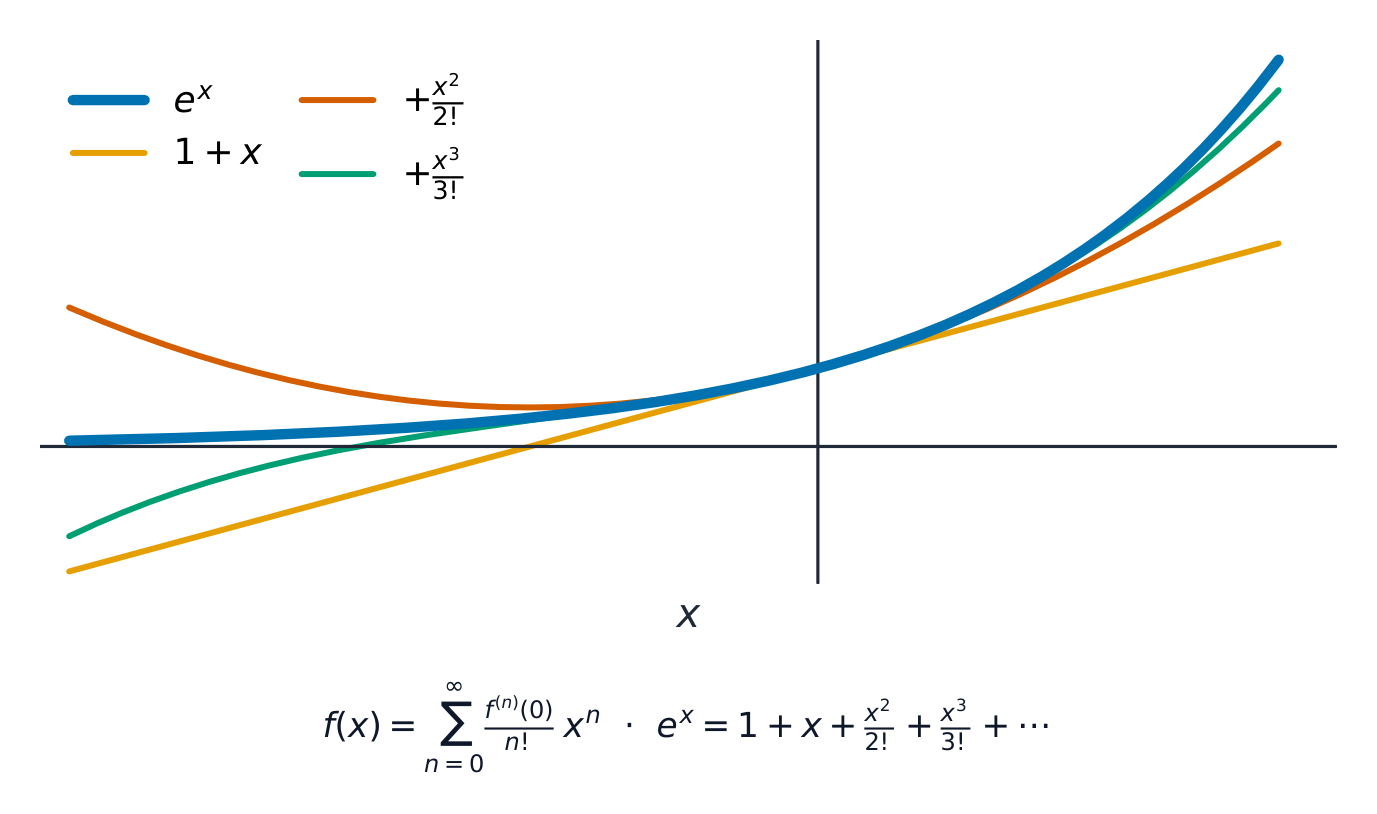
    $$f(x) = f(0) + f'(0)\,x + \frac{f''(0)}{2!}\,x^2 + \frac{f'''(0)}{3!}\,x^3 + \cdots$$
    For example $e^x = 1 + x + \dfrac{x^2}{2!} + \dfrac{x^3}{3!} + \cdots$

    Worked example. Find the Maclaurin series of $f(x) = \ln(1+x)$ up to the term in $x^3$.

    $f(0) = 0$; $f'(x) = \dfrac{1}{1+x}$ so $f'(0) = 1$; $f''(x) = \dfrac{-1}{(1+x)^2}$ so $f''(0) = -1$; $f'''(x) = \dfrac{2}{(1+x)^3}$ so $f'''(0) = 2$. Substituting into the series:

    $$\ln(1+x) = x - \frac{x^2}{2} + \frac{x^3}{3} - \cdots$$
    ไทย

    ตอนนี้คุณสามารถหาอนุพันธ์ของฟังก์ชันไฮเปอร์โบลิกและฟังก์ชันผกผัน $\sin^{-1}x$, $\tan^{-1}x$, $\sinh^{-1}x$ เป็นต้น คุณสามารถหา $\dfrac{d^2y}{dx^2}$ สำหรับโค้งที่กำหนดโดยทางอ้อมหรือแบบพารามิترได้เช่นกัน

    อนุกรมมาคลอริน (Maclaurin's series) เขียนฟังก์ชันให้อยู่ในรูปอนุกรมกำลัง:

    $$f(x) = f(0) + f'(0)\,x + \frac{f''(0)}{2!}\,x^2 + \frac{f'''(0)}{3!}\,x^3 + \cdots$$
    ตัวอย่างเช่น $e^x = 1 + x + \dfrac{x^2}{2!} + \dfrac{x^3}{3!} + \cdots$

    curve e^x พร้อมการประมาณด้วยพหุนามสามแบบที่มีดีกรีเพิ่มขึ้น
    การเพิ่มพจน์มากขึ้นทำให้พหุนามตรงกับ $e^x$ ได้ในช่วงกว้างขึ้นรอบ $x=0$

    ตัวอย่างวิธีทำ. หา Maclaurin series ของ $f(x) = \ln(1+x)$ ไปจนถึงพจน์ที่มี $x^3$

    $f(0) = 0$; $f'(x) = \dfrac{1}{1+x}$ ดังนั้น $f'(0) = 1$; $f''(x) = \dfrac{-1}{(1+x)^2}$ ดังนั้น $f''(0) = -1$; $f'''(x) = \dfrac{2}{(1+x)^3}$ ดังนั้น $f'''(0) = 2$. แทนค่าลงในอนุกรม:

    $$\ln(1+x) = x - \frac{x^2}{2} + \frac{x^3}{3} - \cdots$$
    Explore · ⁨สำรวจ⁩

    The gradient at a point · ⁨ความชันที่จุดหนึ่ง⁩

    gradient = dy/dx

    The derivative is the slope of the tangent, however exotic the function. · ⁨อนุพันธ์ คือความชันของ เส้นสัมผัส ไม่ว่าฟังก์ชันนั้นจะซับซ้อนแค่ไหน⁩

    Vocabulary · ⁨คำศัพท์⁩ Train · ⁨ฝึกฝน⁩
    English ไทย
    Maclaurin's series/məˈklɔːrɪnz ˈsɪəriːz/ อนุกรม Maclaurin
    Watch lesson · ⁨ดูบทเรียน⁩
    2.4

    Integration · ⁨การหาอินทิกรัล (Integration)⁩

    Syllabus · ⁨หลักสูตร⁩
    English
    Candidates should be able to: Notes and examples
    • integrate hyperbolic functions and recognise integrals of functions of the form $\frac{1}{\sqrt{a^2 - x^2}}$, $\frac{1}{\sqrt{x^2 + a^2}}$ and $\frac{1}{\sqrt{x^2 - a^2}}$, and integrate associated functions using trigonometric substitutions or hyperbolic substitutions as appropriate Including use of completing the square where necessary, e.g. to integrate $\frac{1}{\sqrt{x^2 + x}}$.
    • derive and use reduction formulae for the evaluation of definite integrals e.g. $\int_0^{\frac{1}{2}\pi} \sin^n x \text{ d}x$, $\int_0^1 \text{e}^{-x}(1-x)^n \text{ d}x$. In harder cases hints may be given, e.g. $\int_0^{\frac{1}{4}\pi} \sec^n x \text{ d}x$ by considering $\frac{\text{d}}{\text{d}x}(\tan x \sec^n x)$.
    • understand how the area under a curve may be approximated by areas of rectangles, and use rectangles to estimate or set bounds for the area under a curve or to derive inequalities or limits concerning sums Questions may involve either rectangles of unit width or rectangles whose width can tend to zero, e.g. $1 + \ln n > \sum_{r=1}^n \frac{1}{r} > \ln(n+1)$, $\sum_{r=1}^n \frac{1}{n}\left(1 + \frac{r}{n}\right)^{-1} \approx \int_0^1 (1+x)^{-1} \text{ d}x$. continued
    • use integration to find – arc lengths for curves with equations in Cartesian coordinates, including the use of a parameter, or in polar coordinates – surface areas of revolution about one of the axes for curves with equations in Cartesian coordinates, including the use of a parameter. Any questions involving integration may require techniques from Cambridge International A Level Mathematics (9709) applied to more difficult cases, e.g. integration by parts for $\int e^x \sin x \mathrm{d}x$, or use of the substitution $t = \tan \frac{1}{2}x$. Surface areas of revolution for curves with equations in polar coordinates will not be required.
    ไทย
    ผู้เข้าสอบควรสามารถ: หมายเหตุและตัวอย่าง
    • หาปริณิยของ ฟังก์ชันไฮเปอร์บอลิก และระบุปริณิยของฟังก์ชันในรูป $\frac{1}{\sqrt{a^2 - x^2}}$, $\frac{1}{\sqrt{x^2 + a^2}}$ และ $\frac{1}{\sqrt{x^2 - a^2}}$, และหาปริณิยของฟังก์ชันที่เกี่ยวข้องโดยใช้ การแทนค่าตรีโกณมิติ หรือ การแทนค่าไฮเปอร์บอลิก ตามความเหมาะสม รวมถึงการใช้ การเติมเต็มกำลังสอง เมื่อจำเป็น เช่น เพื่อหาปริณิยของ $\frac{1}{\sqrt{x^2 + x}}$
    • สร้างและใช้ สูตรลดรูป เพื่อหาค่าของปริณิยจำกัด เช่น $\int_0^{\frac{1}{2}\pi} \sin^n x \text{ d}x$, $\int_0^1 \text{e}^{-x}(1-x)^n \text{ d}x$ ในกรณีที่ยากขึ้นอาจมีคำแนะนำ เช่น $\int_0^{\frac{1}{4}\pi} \sec^n x \text{ d}x$ โดยการพิจารณา $\frac{\text{d}}{\text{d}x}(\tan x \sec^n x)$
    • เข้าใจว่าพื้นที่ใต้กราฟสามารถประมาณได้ด้วยพื้นที่สี่เหลี่ยมผืนผ้า และใช้สี่เหลี่ยมผืนผ้าเพื่อประมาณหรือกำหนดขอบเขตของพื้นที่ใต้กราฟ หรือเพื่อสร้างอสมการหรือลิมิตเกี่ยวกับผลบวก คำถามอาจเกี่ยวข้องกับสี่เหลี่ยมผืนผ้าที่มีความกว้างเป็นหน่วยเดียวหรือสี่เหลี่ยมผืนผ้าwhose width สามารถเข้าใกล้ศูนย์ได้ เช่น $1 + \ln n > \sum_{r=1}^n \frac{1}{r} > \ln(n+1)$, $\sum_{r=1}^n \frac{1}{n}\left(1 + \frac{r}{n}\right)^{-1} \approx \int_0^1 (1+x)^{-1} \text{ d}x$. ต่อไป
    ใช้ การหาปริณิย เพื่อหา – ความยาวส่วนโค้งสำหรับกราฟที่มีสมการในพิกัดคาร์ทีเซียน รวมถึงการใช้พารามิเตอร์, หรือในพิกัดขั้ว – พื้นที่ผิวของการหมุนรอบแกนใดแกนหนึ่งของกราฟที่มีสมการในพิกัดคาร์ทีเซียน รวมถึงการใช้พารามิเตอร์ คำถามใดๆ ที่เกี่ยวข้องกับการหาปริณิยอาจต้องใช้เทคนิคจาก Cambridge International A Level Mathematics (9709) กับกรณีที่ยากขึ้น เช่น การหาปริณิยด้วยการแบ่งส่วน (integration by parts) สำหรับ $\int e^x \sin x \mathrm{d}x$, หรือการใช้การแทนค่า $t = \tan \frac{1}{2}x$ พื้นที่ผิวของการหมุนสำหรับกราฟที่มีสมการในพิกัดขั้วจะไม่ต้องการ

    Source: Cambridge International syllabus · ⁨แหล่งที่มา: หลักสูตร Cambridge International⁩

    English

    Learn these standard integrals:

    $$\int \frac{1}{a^2 + x^2}\,dx = \frac{1}{a}\tan^{-1}\frac{x}{a} + C, \qquad \int \frac{1}{\sqrt{a^2 - x^2}}\,dx = \sin^{-1}\frac{x}{a} + C.$$
    A trigonometric substitution, a hyperbolic substitution, or completing the square 配方法 in the denominator handles related forms. A reduction formula 递推公式 links an integral $I_n$ to $I_{n-1}$, so you can work down step by step. Integration also gives the arc length 弧长 of a curve and the surface area of revolution 旋转曲面面积 when a curve is turned about an axis.

    Worked example. Find $\displaystyle\int \frac{1}{\sqrt{4 - x^2}}\,dx$.

    Here $a^2 = 4$, so $a = 2$ and

    $$\int \frac{1}{\sqrt{4 - x^2}}\,dx = \sin^{-1}\frac{x}{2} + C.$$

    Bounding a sum by an integral. Draw rectangles of unit width under, or over, a decreasing curve such as $y=\frac1x$. Each rectangle of height $\frac1r$ is trapped between two integral strips, so summing gives

    $$\ln(n+1) < \sum_{r=1}^{n}\frac1r < 1 + \ln n.$$
    Shrinking the rectangle width to $\frac1n\to 0$ turns such a sum into a Riemann sum 黎曼和 that equals the integral in the limit, e.g. $\displaystyle\lim_{n\to\infty}\frac1n\sum_{r=1}^{n}f\!\left(\frac{r}{n}\right)=\int_0^1 f(x)\,dx$.

    ไทย

    จำอินทิกรัลมาตรฐานเหล่านี้:

    $$\int \frac{1}{a^2 + x^2}\,dx = \frac{1}{a}\tan^{-1}\frac{x}{a} + C, \qquad \int \frac{1}{\sqrt{a^2 - x^2}}\,dx = \sin^{-1}\frac{x}{a} + C.$$
    การแทนค่าตรีโกณมิติ, การแทนค่าไฮเปอร์โบลิก, หรือ การเติมให้สมบูรณ์กำลังสอง (completing the square) ในตัวส่วน สามารถจัดการกับรูปแบบที่เกี่ยวข้องได้ สูตรลดรูป (reduction formula) เชื่อมโยงอินทิกรัล $I_n$ กับ $I_{n-1}$ ทำให้คุณสามารถคำนวณทีละขั้นได้ การอินทิเกรตยังให้ ความยาวส่วนโค้ง (arc length) ของ曲线และ พื้นที่ผิวจากการหมุน (surface area of revolution) เมื่อcurve หมุนรอบแกน

    ตัวอย่างมีคำตอบ. หา $\displaystyle\int \frac{1}{\sqrt{4 - x^2}}\,dx$.

    ที่นี่ $a^2 = 4$, ดังนั้น $a = 2$ และ

    $$\int \frac{1}{\sqrt{4 - x^2}}\,dx = \sin^{-1}\frac{x}{2} + C.$$

    การจำกัดผลรวมด้วยอินทิกรัล. วาดสี่เหลี่ยมผืนผ้าที่มีความกว้างหนึ่งหน่วยใต้หรือเหนือ curve ที่ลดลงเช่น $y=\frac1x$. สี่เหลี่ยมผืนผ้าแต่ละอันมีความสูง $\frac1r$ ถูกขังอยู่ระหว่างแถบอินทิกรัลสองแถบ ดังนั้นเมื่อรวมกันจะได้

    $$\ln(n+1) < \sum_{r=1}^{n}\frac1r < 1 + \ln n.$$
    การหดขนาดความกว้างของสี่เหลี่ยมผืนผ้าให้เหลือ $\frac1n\to 0$ จะเปลี่ยนผลรวมดังกล่าวให้เป็น Riemann sum ซึ่งเท่ากับอินทิกรัลในลิมิต เช่น $\displaystyle\lim_{n\to\infty}\frac1n\sum_{r=1}^{n}f\!\left(\frac{r}{n}\right)=\int_0^1 f(x)\,dx$

    Explore · ⁨สำรวจ⁩

    The area under the curve · ⁨พื้นที่ใต้กราฟ⁩

    area = ∫ f(x) dx

    Every integral measures the area under the curve — drag the limits. · ⁨ทุกอินทิกรัลวัด พื้นที่ ภายใต้กราฟ — ลากขอบเขต⁩

    Vocabulary · ⁨คำศัพท์⁩ Train · ⁨ฝึกฝน⁩
    English ไทย
    completing the square/kəmˈpliːtɪŋ ðə skweə/ การเติมกำลังสองสมบูรณ์
    reduction formula/rɪˈdʌkʃn ˈfɔːmjʊlə/ สูตรลดรูป
    arc length/ɑːk leŋθ/ ความยาวส่วนโค้ง
    surface area of revolution/ˈsɜːfɪs ˈeərɪə ɒv ˌrevəˈluːʃn/ พื้นที่ผิวจากการหมุน
    Riemann sum/ˈriːmən sʌm/ ผลรวมรีแมน
    complex number/ˈkɒmpleks ˈnʌmbə/ จำนวนเชิงซ้อน
    Watch lesson · ⁨ดูบทเรียน⁩
    2.5

    Complex numbers · ⁨จำนวนเชิงซ้อน (Complex numbers)⁩

    Syllabus · ⁨หลักสูตร⁩
    English
    Candidates should be able to: Notes and examples
    • understand de Moivre’s theorem, for a positive or negative integer exponent, in terms of the geometrical effect of multiplication and division of complex numbers
    • prove de Moivre’s theorem for a positive integer exponent e.g. by induction.
    • use de Moivre’s theorem for a positive or negative rational exponent e.g. expressing $\cos 5\theta$ in terms of $\cos \theta$ or $\tan 5\theta$ in terms of $\tan \theta$.
    – to express trigonometrical ratios of multiple angles in terms of powers of trigonometrical ratios of the fundamental angle e.g. expressing $\sin^6 \theta$ in terms of $\cos 2\theta$, $\cos 4\theta$ and $\cos 6\theta$.
    – to express powers of $\sin \theta$ and $\cos \theta$ in terms of multiple angles
    – in the summation of series e.g. using the '$C + \mathrm{i}S$' method to sum series such as $\sum_{r=1}^{n} \binom{n}{r} \sin r\theta$.
    – in finding and using the $n$th roots of unity.
    ไทย
    ผู้เข้าสอบควรสามารถ: หมายเหตุและตัวอย่าง
    เข้าใจ ทฤษฎีบท de Moivre, สำหรับเลขชี้กำลังเป็นจำนวนเต็มบวกหรือลบ, ในแง่ของผลกระทบทางเรขาคณิตของการคูณและการหาร จำนวนเชิงซ้อน
    พิสูจน์ ทฤษฎีบท de Moivre สำหรับเลขชี้กำลังเป็นจำนวนเต็มบวก เช่น โดยใช้การพิสูจน์ด้วยวิธีอุปนัย (induction)
    ใช้ ทฤษฎีบท de Moivre สำหรับเลขชี้กำลังเป็นจำนวนตรรกยะบวกหรือลบ เช่น การแสดง $\cos 5\theta$ ในรูป $\cos \theta$ หรือ $\tan 5\theta$ ในรูป $\tan \theta$
    – เพื่อแสดงอัตราส่วนตรีโกณมิติของมุมหลายเท่าในรูปกำลังของอัตราส่วนตรีโกณมิติของมุมพื้นฐาน เช่น การแสดง $\sin^6 \theta$ ในรูป $\cos 2\theta$, $\cos 4\theta$ และ $\cos 6\theta$
    – เพื่อแสดงกำลังของ $\sin \theta$ และ $\cos \theta$ ในรูปมุมหลายเท่า
    – ในการหาผลบวกของอนุกรม เช่น การใช้วิธี '$C + \mathrm{i}S$' เพื่อหาผลบวกอนุกรมเช่น $\sum_{r=1}^{n} \binom{n}{r} \sin r\theta$
    – ในการหาและใช้ $n$th รากของเอกฐาน (roots of unity)

    Source: Cambridge International syllabus · ⁨แหล่งที่มา: หลักสูตร Cambridge International⁩

    English
    The nth roots of unity form a polygon
    Multiplying complex numbers: lengths multiply, angles add
    Multiplying by i is a rotation

    A complex number 复数 in polar form is $z = r(\cos\theta + i\sin\theta)$. De Moivre's theorem 棣莫弗定理 says that for any integer $n$,

    $$(\cos\theta + i\sin\theta)^n = \cos n\theta + i\sin n\theta.$$
    It is used to expand $\cos n\theta$ and $\sin n\theta$ in powers, to sum series, and to find the $n$ roots of unity 单位根 (the solutions of $z^n = 1$, equally spaced around the unit circle).

    Worked example. Use de Moivre's theorem to express $\cos 3\theta$ in terms of $\cos\theta$.

    Take the real part of $(\cos\theta + i\sin\theta)^3 = \cos 3\theta + i\sin 3\theta$:

    $$\cos 3\theta = \cos^3\theta - 3\cos\theta\sin^2\theta = \cos^3\theta - 3\cos\theta(1 - \cos^2\theta) = 4\cos^3\theta - 3\cos\theta.$$

    ไทย
    รากที่ n ของเอกฐานประกอบด้วยรูปหลายเหลี่ยม
    การคูณจำนวนเชิงซ้อน: ความยาวคูณกัน มุมบวกกัน
    การคูณด้วย i คือการหมุน
    หัวบรอกโคลี Romanesque แสดงเกลียวที่มีลักษณะซ้ำตัวเอง
    ลวดลายที่เหมือนตัวเองอย่างบรอกโคลี Romanesco เกิดจากการทำซ้ำฟังก์ชันในระนาบเชิงซ้อน

    จำนวนเชิงซ้อนในรูปแบบขั้วคือ $z = r(\cos\theta + i\sin\theta)$. ทฤษฎีบทเดโมวัวร์ (De Moivre's theorem) กล่าวว่าสำหรับจำนวนเต็ม $n$ ใดๆ,

    $$(\cos\theta + i\sin\theta)^n = \cos n\theta + i\sin n\theta.$$
    ใช้เพื่อขยาย $\cos n\theta$ และ $\sin n\theta$ เป็นกำลัง เพื่อรวมอนุกรม และหา $n$ รากของเอกฐาน (roots of unity) (คำตอบของ $z^n = 1$, เรียงห่างกันเท่าๆ รอบวงกลมหน่วย)

    จุดห้าจุดกระจายตัวเท่าๆ บนวงกลมหน่วยบนแผนภาพ Argand
    คำตอบทั้งห้าของ $z^5=1$ กระจายห่างกัน $72^\circ$ เท่าๆ บนวงกลมหน่วย

    ตัวอย่างวิธีทำ. ใช้ทฤษฎีบทเดโมวัวร์เพื่อเขียน $\cos 3\theta$ ในเทอมของ $\cos\theta$

    lấyส่วนจริงของ $(\cos\theta + i\sin\theta)^3 = \cos 3\theta + i\sin 3\theta$:

    $$\cos 3\theta = \cos^3\theta - 3\cos\theta\sin^2\theta = \cos^3\theta - 3\cos\theta(1 - \cos^2\theta) = 4\cos^3\theta - 3\cos\theta.$$

    Explore · ⁨สำรวจ⁩

    The Argand diagram

    Drag the point to explore modulus and argument — the language of complex numbers in polar (modulus–argument) form. · ⁨ลากจุดเพื่อสำรวจโมดูลัสและอาร์กิวเมนต์ — ภาษาของจำนวนเชิงซ้อนในรูปแบบเชิงขั้ว (โมดูลัส-อาร์กิวเมนต์)⁩

    Vocabulary · ⁨คำศัพท์⁩ Train · ⁨ฝึกฝน⁩
    English ไทย
    De Moivre's theorem/də ˈmɔɪvəz ˈθɪərəm/ ทฤษฎีบท De Moivre
    roots of unity/ruːts ɒv ˈjuːnɪti/ รากของหน่วย
    Watch lesson · ⁨ดูบทเรียน⁩
    2.6

    Differential equations · ⁨สมการเชิงอนุพันธ์ (Differential equations)⁩

    Syllabus · ⁨หลักสูตร⁩
    English
    Candidates should be able to: Notes and examples
    • find an integrating factor for a first order linear differential equation, and use an integrating factor to find the general solution e.g. $\frac{\mathrm{d}y}{\mathrm{d}x} - 2y = x^2$, $x\frac{\mathrm{d}y}{\mathrm{d}x} - y = x^4$, $\frac{\mathrm{d}y}{\mathrm{d}x} + y\coth x = \cosh x$.
    • recall the meaning of the terms 'complementary function' and 'particular integral' in the context of linear differential equations, and recall that the general solution is the sum of the complementary function and a particular integral
    find the complementary function for a first or second order linear differential equation with constant coefficients For second order equations, including the cases where the auxiliary equation has distinct real roots, a repeated real root or conjugate complex roots.
    recall the form of, and find, a particular integral for a first or second order linear differential equation in the cases where a polynomial or $ae^{bx}$ or $a\cos px + b\sin px$ is a suitable form, and in other simple cases find the appropriate coefficient(s) given a suitable form of particular integral e.g. evaluate $k$ given that $kx \cos 2x$ is a particular integral of
    $$\frac{\text{d}^2y}{\text{d}x^2} + 4y = \sin 2x$$
    .
    use a given substitution to reduce a differential equation to a first or second order linear equation with constant coefficients or to a first order equation with separable variables e.g. the substitution $x = e^t$ to reduce to linear form a differential equation with terms of the form
    $$ax^2\frac{\text{d}^2y}{\text{d}x^2} + bx\frac{\text{d}y}{\text{d}x} + cy$$
    , or the substitution $y = ux$ to reduce
    $$\frac{\text{d}y}{\text{d}x} = \frac{x+y}{x-y}$$
    to separable form.
    use initial conditions to find a particular solution to a differential equation, and interpret a solution in terms of a problem modelled by a differential equation.
    ไทย
    ผู้เข้าสอบควรสามารถ: หมายเหตุและตัวอย่าง
    หา ตัวประกอบบูรณาการ (integrating factor) สำหรับ สมการเชิงอนุพันธ์เชิงเส้นอันดับหนึ่ง และใช้ ตัวประกอบบูรณาการ เพื่อหาคำตอบทั่วไป เช่น $\frac{\mathrm{d}y}{\mathrm{d}x} - 2y = x^2$, $x\frac{\mathrm{d}y}{\mathrm{d}x} - y = x^4$, $\frac{\mathrm{d}y}{\mathrm{d}x} + y\coth x = \cosh x$
    จำความหมายของคำว่า 'ฟังก์ชันเสริม (complementary function)' และ 'อินทิกรัลเฉพาะ (particular integral)' ในบริบทของ สมการเชิงอนุพันธ์เชิงเส้น, และจำได้ว่าคำตอบทั่วไปคือผลบวกของ ฟังก์ชันเสริม และ อินทิกรัลเฉพาะ
    หาค่า ฟังก์ชันเสริม สำหรับสมการเชิงอนุพันธ์เชิงเส้นอันดับหนึ่งหรืออันดับสองที่มีสัมประสิทธิ์คงที่ สำหรับสมการอันดับสอง รวมถึงกรณีที่ สมการช่วย (auxiliary equation) มีรากจริงที่แตกต่างกัน รากจริงซ้ำ หรือรากจินตภาพคู่สม
    จำรูปแบบและหาค่า อินทิกรัลเฉพาะ สำหรับสมการเชิงอนุพันธ์เชิงเส้นอันดับหนึ่งหรืออันดับสองในกรณีที่พหุนามหรือ $ae^{bx}$ หรือ $a\cos px + b\sin px$ เป็นรูปแบบที่เหมาะสม, และในกรณีอื่นๆ ที่เรียบง่าย ให้หาสัมประสิทธิ์ที่เหมาะสมให้เมื่อทราบรูปแบบของอินทิกรัลเฉพาะ เช่น คำนวณ $k$ โดยกำหนดให้ $kx \cos 2x$ เป็นอินทิกรัลเฉพาะของ
    $$\frac{\text{d}^2y}{\text{d}x^2} + 4y = \sin 2x$$
    ใช้ การแทนค่า ที่กำหนดให้เพื่อลดรูปสมการเชิงอนุพันธ์ให้เป็นสมการเชิงเส้นอันดับหนึ่งหรืออันดับสองที่มีสัมประสิทธิ์คงที่ หรือให้เป็นสมการอันดับหนึ่งที่มี ตัวแปรแยกได้ (separable variables) เช่น การแทนค่า $x = e^t$ เพื่อลดรูปสมการเชิงอนุพันธ์ที่มีพจน์ในรูป
    $$ax^2\frac{\text{d}^2y}{\text{d}x^2} + bx\frac{\text{d}y}{\text{d}x} + cy$$
    ให้เป็นรูปเชิงเส้น, หรือการแทนค่า $y = ux$ เพื่อลด
    $$\frac{\text{d}y}{\text{d}x} = \frac{x+y}{x-y}$$
    ให้เป็นรูปที่แยกตัวแปรได้
    ใช้ เงื่อนไขเริ่มต้น เพื่อหาค่า คำตอบเฉพาะ ของสมการเชิงอนุพันธ์, และตีความคำตอบในแง่ของปัญหาที่ถูกจำลองด้วยสมการเชิงอนุพันธ์

    Source: Cambridge International syllabus · ⁨แหล่งที่มา: หลักสูตร Cambridge International⁩

    English

    For a first order linear equation $\dfrac{dy}{dx} + P(x)\,y = Q(x)$, multiply by the integrating factor 积分因子 $\mu = e^{\int P\,dx}$. The left side then becomes $\dfrac{d}{dx}(\mu y)$, so you can integrate directly.

    For a linear equation with constant coefficients, the general solution 通解 is the sum of two parts: the complementary function 余函数 (the solution of the equation with the right side set to $0$, found from the auxiliary equation) and a particular integral 特积分 (any one solution of the full equation). Initial conditions then fix the constants to give the particular solution 特解; simpler equations with separable variables 可分离变量 are integrated directly.

    Worked example. Solve $\dfrac{dy}{dx} + 2y = e^x$.

    The integrating factor is $\mu = e^{\int 2\,dx} = e^{2x}$. Multiplying through gives $\dfrac{d}{dx}\!\left(y\,e^{2x}\right) = e^{3x}$, so

    $$y\,e^{2x} = \tfrac13 e^{3x} + C \;\Rightarrow\; y = \tfrac13 e^x + C e^{-2x}.$$

    Second order, constant coefficients. For $\dfrac{d^2y}{dx^2}+b\dfrac{dy}{dx}+cy=f(x)$, solve the auxiliary equation 辅助方程 $m^2+bm+c=0$. The complementary function depends on its roots:

    • two distinct real roots $m_1,m_2$: $y=Ae^{m_1x}+Be^{m_2x}$;
    • a repeated root $m$: $y=(A+Bx)e^{mx}$;
    • complex roots $p\pm qi$: $y=e^{px}(A\cos qx+B\sin qx)$.

    Then add a particular integral by trying a form matching $f(x)$ (a polynomial, $ae^{bx}$, or $a\cos px+b\sin px$); if that trial already appears in the complementary function, multiply it by $x$.

    Worked example. Solve $\dfrac{d^2y}{dx^2}-4\dfrac{dy}{dx}+4y=0$. The auxiliary equation $m^2-4m+4=(m-2)^2=0$ has a repeated root $m=2$, so $y=(A+Bx)e^{2x}$.

    ไทย

    สำหรับสมการเชิงเส้นอันดับหนึ่ง $\dfrac{dy}{dx} + P(x)\,y = Q(x)$, คูณด้วย ตัวประกอบอินทิเกรต (integrating factor) $\mu = e^{\int P\,dx}$. ด้านซ้ายจะกลายเป็น $\dfrac{d}{dx}(\mu y)$, sehinggaคุณสามารถอินทิเกรตโดยตรง

    สำหรับสมการเชิงเส้นสัมประสิทธิ์คงที่ คำตอบทั่วไป (general solution) คือผลบวกของสองส่วน: ฟังก์ชันเสริม (complementary function) (คำตอบของสมการwhen side kanan ตั้งเป็น $0$, หาได้จาก auxiliary equation) และ อินทิกรัลเฉพาะ (particular integral) (คำตอบใดคำตอบหนึ่งของสมการเต็ม) เงื่อนไขเริ่มต้น (Initial conditions) จะกำหนดค่าคงที่เพื่อให้ได้ คำตอบเฉพาะ (particular solution); สมการที่ง่ายกว่าที่มี ตัวแปรแยกได้ (separable variables) จะอินทิเกรตโดยตรง

    ตารางของส่วนเอียงสั้นๆ พร้อมเส้นโซลูชันสองเส้นวิ่งผ่านตารางนั้น
    โค้งคำตอบจะติดตามสนามความชัน (slope field) โดยสัมผัสกับส่วนประกอบเล็กๆ ทุกที่

    ตัวอย่างวิธีทำ. แก้ $\dfrac{dy}{dx} + 2y = e^x$

    ตัวประกอบอินทิเกรตคือ $\mu = e^{\int 2\,dx} = e^{2x}$. คูณทั่วแล้วจะได้ $\dfrac{d}{dx}\!\left(y\,e^{2x}\right) = e^{3x}$, ดังนั้น

    $$y\,e^{2x} = \tfrac13 e^{3x} + C \;\Rightarrow\; y = \tfrac13 e^x + C e^{-2x}.$$

    สมการเชิงอนุพันธ์อันดับสอง สัมประสิทธิ์คงที่ สำหรับ $\dfrac{d^2y}{dx^2}+b\dfrac{dy}{dx}+cy=f(x)$ ให้แก้ สมการช่วย $m^2+bm+c=0$. ฟังก์ชันเสริมขึ้นอยู่กับรากของสมการนี้:

    • รากจริงที่แตกต่างกันสองค่า $m_1,m_2$: $y=Ae^{m_1x}+Be^{m_2x}$;
    • รากซ้ำ $m$: $y=(A+Bx)e^{mx}$;
    • รากเชิงซ้อน $p\pm qi$: $y=e^{px}(A\cos qx+B\sin qx)$.

    จากนั้นเพิ่มผลเฉลยเฉพาะโดยลองใช้รูปแบบที่ตรงกับ $f(x)$ (พหุนาม, $ae^{bx}$, หรือ $a\cos px+b\sin px$); หากรูปแบบทดสอบนั้นปรากฏอยู่ในฟังก์ชันเสริมอยู่แล้ว ให้ คูณด้วย $x$

    ตัวอย่างวิธีทำ. แก้ $\dfrac{d^2y}{dx^2}-4\dfrac{dy}{dx}+4y=0$. สมการช่วย $m^2-4m+4=(m-2)^2=0$ มีรากซ้ำ $m=2$ ดังนั้น $y=(A+Bx)e^{2x}$.

    Explore · ⁨สำรวจ⁩

    Differential equations · ⁨สมการเชิงอนุพันธ์⁩

    dy/dx = a y

    The equation sets the slope everywhere; the solution follows those slopes. · ⁨สมการกำหนด slope ทุกที่; คำตอบ จะตาม slope เหล่านี้⁩

    Vocabulary · ⁨คำศัพท์⁩ Train · ⁨ฝึกฝน⁩
    English ไทย
    integrating factor/ˈɪntɪɡreɪtɪŋ ˈfæktə/ ตัวประกอบอินทิเกรต
    general solution/ˈdʒenərəl səˈluːʃn/ คำตอบทั่วไป
    complementary function/ˌkɒmplɪˈmentəri ˈfʌŋkʃn/ ฟังก์ชันเสริม
    particular integral/pəˈtɪkjʊlə ˈɪntɪɡrəl/ อินทิกรัลเฉพาะ
    particular solution/pəˈtɪkjʊlə səˈluːʃn/ คำตอบเฉพาะ
    separable variables/ˈsepərəbl ˈveərɪəblz/ ตัวแปรแยกได้
    auxiliary equation/ɔːkˈsɪlɪəri ɪˈkweɪʒn/ สมการช่วย
    2.6

    Exam tips · ⁨ข้อแนะนำสำหรับการสอบ⁩

    English
    • Learn the hyperbolic identities and derivatives, and use the inverse hyperbolic functions in integration.
    • Solve a linear differential equation as complementary function $+$ particular integral, then apply the boundary conditions.
    • Use de Moivre's theorem for powers and roots of complex numbers and to derive trigonometric identities.
    • Reduce an integral to a standard form by a stated substitution.
    ไทย
    • จำ เอกลักษณ์ forecast hyperbolic และอนุพันธ์ของมันได้ และใช้ฟังก์ชัน forecast hyperbolic แบบผกผันในการหาปริพันธ์
    • แก้ สมการเชิงอนุพันธ์เชิงเส้น โดยหาฟังก์ชันเสริม $+$ ผลเฉลยเฉพาะ แล้วใช้เงื่อนไขขอบเขต
    • ใช้ ทฤษฎีบท de Moivre สำหรับเลขยกกำลังและรากของจำนวนเชิงซ้อน และการพิสูจน์เอกลักษณ์ตรีโกณมิติ
    • ลดรูปปริพันธ์ให้อยู่ในมาตรฐาน bằng การแทนตัวแปรที่กำหนดให้
  • 3

    Further Mechanics · ⁨กลศาสตร์เพิ่มเติม⁩

    Watch lesson · ⁨ดูบทเรียน⁩
    English

    This handout covers Topic 3: Further Mechanics 进阶力学. It extends mechanics to projectiles, rigid bodies, circular motion, elastic strings, variable forces and collisions. Take $g = 10\ \text{m s}^{-2}$.

    ไทย

    เอกสารฉบับนี้ครอบคลุมหัวข้อที่ 3: กลศาสตร์ขั้นสูง ซึ่งขยายเนื้อหากลศาสตร์ไปยังวัตถุโปรเจกไทล์ วัตถุแข็งเกร็ง การเคลื่อนที่วงกลม สายยางยืด แรงแปรผัน และการชนกัน เลือก $g = 10\ \text{m s}^{-2}$

    3.1

    Motion of a projectile · ⁨การเคลื่อนที่ของวัตถุโปรเจกไทล์⁩

    Syllabus · ⁨หลักสูตร⁩
    English
    Candidates should be able to: Notes and examples
    • model the motion of a projectile as a particle moving with constant acceleration and understand any limitations of the model Vector methods are not required
    • use horizontal and vertical equations of motion to solve problems on the motion of projectiles, including finding the magnitude and direction of the velocity at a given time or position, the range on a horizontal plane and the greatest height reached
    • derive and use the Cartesian equation of the trajectory of a projectile, including problems in which the initial speed and/or angle of projection may be unknown. Knowledge of the 'bounding parabola' for accessible points is not included.
    ไทย
    ผู้เข้าสอบควรสามารถ: หมายเหตุและตัวอย่าง
    📐 สร้างแบบจำลองการเคลื่อนที่ของ วัตถุถูกยิง ว่าเป็นอนุภาคที่เคลื่อนที่ด้วยความเร่งคงที่ และเข้าใจข้อจำกัดของแบบจำลอง ไม่จำเป็นต้องใช้วิธีการเวกเตอร์
    📐 ใช้สมการการเคลื่อนที่แนวนอนและแนวตั้งเพื่อแก้ปัญหาเกี่ยวกับการเคลื่อนที่ของวัตถุถูกยิง, รวมถึงการหาขนาดและทิศทางของความเร็ว ณ เวลาหรือตำแหน่งที่กำหนด, ระยะทางบนระนาบแนวนอน และความสูงสูงสุดที่ถึงได้
    • หาและใช้ สมการคาร์ทีเซียน ของเส้นทางการเคลื่อนที่ของวัตถุที่กระโดดขึ้นในอากาศ รวมถึงปัญหาที่มีความเร็วเริ่มต้นและ/หรือมุมในการยิงไม่ทราบค่า ไม่รวมถึงความรู้เกี่ยวกับ 'พาราโบลาจำกัด' สำหรับจุดที่เข้าถึงได้

    Source: Cambridge International syllabus · ⁨แหล่งที่มา: หลักสูตร Cambridge International⁩

    English
    Dropped vs thrown: falling together

    A projectile 抛射体 moves freely under gravity, so it has constant acceleration 匀加速 $g$ downwards and no horizontal acceleration. Treat the horizontal and vertical motions separately. If it is launched at speed $u$ and angle $\alpha$:

    $$\text{horizontal: } x = u\cos\alpha\,\cdot t, \qquad \text{vertical: } y = u\sin\alpha\,\cdot t - \tfrac12 g t^2.$$
    Eliminating $t$ gives the Cartesian equation 直角坐标方程 of the trajectory 轨迹 (the path), which is a parabola. For a fixed launch speed, all the trajectories lie under a bounding parabola 包络抛物线 (the envelope of reachable points). The range on level ground is $\dfrac{u^2\sin 2\alpha}{g}$ and the greatest height is $\dfrac{u^2\sin^2\alpha}{2g}$.

    Worked example. A ball is thrown at $u = 20\ \text{m s}^{-1}$ at $30^\circ$ to the horizontal. Find the range and greatest height.

    $$\text{range} = \frac{20^2\sin 60^\circ}{10} = 40\times 0.866 = 34.6\ \text{m}, \qquad \text{height} = \frac{20^2\sin^2 30^\circ}{2\times 10} = \frac{400\times 0.25}{20} = 5\ \text{m}.$$

    ไทย
    ปล่อย vs ทิ้ง: หล่นพร้อมกัน
    น้ำพวยพุ่งเป็นโค้งในบ่อน้ำใหญ่
    พวยงาน้ำเคลื่อนที่ตามเส้นทางพาราโบลา — การเคลื่อนที่แบบโปรเจกไทล์คลาสสิกภายใต้แรงโน้มถ่วง

    วัตถุ โปรเจกไทล์ เคลื่อนที่อย่างอิสระภายใต้แรงโน้มถ่วง จึงมี ความเร่งคงที่ $g$ ชี้ลงด้านล่างและไม่มีความเร่งแนวนอน พิจารณาการเคลื่อนที่แนวนอนและแนวตั้งแยกจากกัน หากมันถูกยิงด้วยความเร็ว $u$ ที่มุม $\alpha$:

    $$\text{horizontal: } x = u\cos\alpha\,\cdot t, \qquad \text{vertical: } y = u\sin\alpha\,\cdot t - \tfrac12 g t^2.$$
    การกำจัด $t$ จะได้ สมการคาร์ทีเซียน ของ เส้นทาง (trajectory) ซึ่งเป็นพาราโบลา สำหรับความเร็วในการยิงคงที่ เส้นทางทั้งหมดจะอยู่ใต้ พาราโบลาค่าจำกัด (bounding parabola; envelope of reachable points) ระยะทางบนพื้นราบคือ $\dfrac{u^2\sin 2\alpha}{g}$ และความสูงสูงสุดคือ $\dfrac{u^2\sin^2\alpha}{2g}$

    เส้นทางพาราโบลาที่แยกความเร็วในการยิงออกเป็นองค์ประกอบแนวนอนและแนวตั้ง
    เส้นทางเป็นพาราโบลา; ความเร็วในการยิง $u$ แยกออกเป็นองค์ประกอบแนวนอนที่คงที่และองค์ประกอบแนวตั้งที่ช้าลงเนื่องจากแรงโน้มถ่วง

    ตัวอย่างวิธีทำ. ขวดยิงด้วยความเร็ว $u = 20\ \text{m s}^{-1}$ ที่มุม $30^\circ$ เทียบกับแนวนอน หาระยะทางและความสูงสูงสุด

    $$\text{range} = \frac{20^2\sin 60^\circ}{10} = 40\times 0.866 = 34.6\ \text{m}, \qquad \text{height} = \frac{20^2\sin^2 30^\circ}{2\times 10} = \frac{400\times 0.25}{20} = 5\ \text{m}.$$

    Explore · ⁨สำรวจ⁩

    Launch a projectile · ⁨ยิงวัตถุ⁩

    Fire the ball, then change the angle and speed. The horizontal motion is steady while gravity pulls it down — together they trace a parabola. Find the angle for the longest range, and try the Moon. · ⁨ยิงลูกบอล แล้วเปลี่ยนมุมและความเร็ว การเคลื่อนที่แนวนอนมีความคงที่ขณะที่แรงโน้มถ่วงดึงลง — ทั้งสองรวมกันสร้างเส้นโค้งพาราโบลา หามุมที่ให้ระยะทางไกลที่สุด และลองทำบนดวงจันทร์⁩

    Vocabulary · ⁨คำศัพท์⁩ Train · ⁨ฝึกฝน⁩
    English ไทย
    Further Mechanics/ˈfɜːðə mɪˈkænɪks/ กลศาสตร์เพิ่มเติม
    projectile/prəˈdʒektaɪl/ วัตถุถูกยิง
    constant acceleration/ˈkɒnstənt əkˌseləˈreɪʃn/ ความเร่งคงที่
    Cartesian equation/kɑːˈtiːzɪən ɪˈkweɪʒn/ สมการคาร์ทีเซียน
    trajectory/trəˈdʒektəri/ เส้นทาง
    bounding parabola/ˈbaʊndɪŋ pəˈræbələ/ พาราโบลาขอบเขต
    3.2

    Equilibrium of a rigid body · ⁨สมดุลของวัตถุแข็งเกร็ง⁩

    Syllabus · ⁨หลักสูตร⁩
    English
    Candidates should be able to: Notes and examples
    • calculate the moment of a force about a point For questions involving coplanar forces only; understanding of the vector nature of moments is not required.
    • use the result that the effect of gravity on a rigid body is equivalent to a single force acting at the centre of mass of the body, and identify the position of the centre of mass of a uniform body using considerations of symmetry
    • use given information about the position of the centre of mass of a triangular lamina and other simple shapes Proofs of results given in the MF19 List of formulae are not required.
    • determine the position of the centre of mass of a composite body by considering an equivalent system of particles Simple cases only, e.g. a uniform L-shaped lamina, or a uniform cone joined at its base to a uniform hemisphere of the same radius.
    • use the principle that if a rigid body is in equilibrium under the action of coplanar forces then the vector sum of the forces is zero and the sum of the moments of the forces about any point is zero, and the converse of this
    • solve problems involving the equilibrium of a single rigid body under the action of coplanar forces, including those involving toppling or sliding.
    ไทย
    ผู้เข้าสอบควรสามารถ: หมายเหตุและตัวอย่าง
    • คำนวณ โมเมนต์ ของแรงรอบจุดหนึ่ง สำหรับข้อสอบที่เกี่ยวข้องกับ แรงระนาบ เท่านั้น; ความเข้าใจในลักษณะเวกเตอร์ของโมเมนต์ไม่จำเป็น
    • ใช้ผลลัพธ์ที่ว่าผลของแรงโน้มถ่วงต่อ ร่างกายแข็ง มีผลเทียบเท่าแรงเดียวกระทำที่ จุดศูนย์กลางมวล ของร่างกาย และระบุตำแหน่งของจุดศูนย์กลางมวลของร่างกายสม่ำเสมอโดยใช้หลักการสมมาตร
    • ใช้ข้อมูลที่กำหนดให้เกี่ยวกับตำแหน่งของจุดศูนย์กลางมวลของแผ่นบางรูปสามเหลี่ยมและรูปร่างเรียบง่ายอื่นๆ การพิสูจน์ผลลัพธ์ที่ระบุไว้ในรายการสูตร MF19 ไม่จำเป็น
    • กำหนดตำแหน่งของจุดศูนย์กลางมวลของ ร่างกายประกอบ โดยพิจารณาจากระบบอนุภาคที่เทียบเท่า กรณีง่ายเท่านั้น เช่น แผ่นบางรูปตัว L สม่ำเสมอ หรือกรวยสม่ำเสมอเชื่อมฐานกับครึ่งทรงกลมสม่ำเสมอที่มีรัศมีเท่ากัน
    • ใช้หลักการที่ว่าถ้าร่างกายแข็งอยู่ใน สมดุล ภายใต้การกระทำของแรงระนาบ แล้วผลรวมของแรงเป็นศูนย์และผลรวมของโมเมนต์ของแรงรอบจุดใดๆ เป็นศูนย์ และกลับด้านของสิ่งนี้
    • แก้ปัญหา涉及到การสมดุลของร่างกายแข็งภายใต้การกระทำของแรงระนาบ بماที่涉及到 การล้ม หรือ การลื่นไถล

    Source: Cambridge International syllabus · ⁨แหล่งที่มา: หลักสูตร Cambridge International⁩

    English

    The moment 力矩 of a force about a point is force $\times$ perpendicular distance; it measures turning effect. The weight of a body acts at its centre of mass 质心, which you can find using symmetry 对称 for a uniform flat shape (a lamina 薄片), or by treating a composite body as a set of particles.

    A rigid body under coplanar forces 共面力 is in equilibrium 平衡 when two conditions both hold: the vector sum of the forces is zero, and the sum of the moments about any point is zero. A body may also be on the edge of toppling 翻倒 (turning over) or sliding 滑动 (slipping).

    Worked example. A uniform beam $AB$ of length $4\ \text{m}$ and weight $100\ \text{N}$ rests on a pivot at $A$. A vertical force $F$ at $B$ keeps it horizontal. Find $F$.

    Take moments about $A$ (the weight acts at the centre, $2\ \text{m}$ from $A$):

    $$F\times 4 = 100\times 2 \;\Rightarrow\; F = 50\ \text{N}.$$

    ไทย

    โมเมนต์ ของแรงรอบจุดหนึ่งคือ แรง $\times$ คูยะ距ตั้งฉาก; เป็นตัววัดผลหมุน น้ำหนักของวัตถุกระทำที่ ศูนย์มวล ซึ่งคุณสามารถหาได้โดยใช้ ความสมมาตร สำหรับรูปร่างแบนเรียบสม่ำเสมอ (แผ่นบาง; lamina), หรือโดยการพิจารณาวัตถุผสมเป็นกลุ่มของอนุภาค

    วัตถุแข็งเกร็งที่อยู่ภายใต้ แรงระนาบ อยู่ในสภาวะ สมดุล เมื่อเงื่อนไขทั้งสองนี้เป็นจริง: ผลรวมเวกเตอร์ของแรงเป็นศูนย์ และผลรวมโมเมนต์รอบจุดใด ๆ เป็นศูนย์ วัตถุนั้นอาจอยู่ในสภาวะใกล้จะ คว่ำ (toppling) หรือ ลื่นไถล (sliding)

    คานบนจุดหมุนที่มีน้ำหนักอยู่ที่ศูนย์กลางและรับแรงที่ปลายอีกด้านหนึ่ง
    การคำนวณโมเมนต์รอบจุดหมุน $A$ ทำให้ผลหมุนสมดุล: $F\times4 = 100\times2$.

    ตัวอย่างวิธีทำ. คานสม่ำเสมอ $AB$ ยาว $4\ \text{m}$ และมีน้ำหนัก $100\ \text{N}$ วางอยู่บนจุดหมุนที่ $A$. แรงตั้งฉาก $F$ ที่ $B$ ทำให้คานอยู่ในแนวนอน หา $F$

    คำนวณโมเมนต์รอบ $A$ (น้ำหนักกระทำที่ศูนย์กลาง, $2\ \text{m}$ จาก $A$):

    $$F\times 4 = 100\times 2 \;\Rightarrow\; F = 50\ \text{N}.$$

    Explore · ⁨สำรวจ⁩

    Equilibrium of forces · ⁨สมดุลของแรง⁩

    resultant = 0 · ⁨ผลรวม = 0⁩

    A body is in equilibrium when the forces add tip-to-tail back to zero. · ⁨วัตถุอยู่ใน สมดุล เมื่อผลรวมของแรง ปลายต่อหัว กลับไปเป็นศูนย์⁩

    Vocabulary · ⁨คำศัพท์⁩ Train · ⁨ฝึกฝน⁩
    English ไทย
    moment/ˈməʊmənt/ ปัจจุบัน
    centre of mass/ˈsentə ɒv mæs/ ศูนย์กลางมวล
    symmetry/ˈsɪmətri/ symmetry
    equilibrium/ˌiːkwɪˈlɪbrɪəm/ จุดดุลยภาพ
    toppling/ˈtɒplɪŋ/ การล้มลง
    sliding/ˈslaɪdɪŋ/ การเลื่อน
    angular speed/ˈæŋɡjʊlə spiːd/ ความเร็วเชิงมุม
    centripetal acceleration/senˈtrɪpɪtl əkˌseləˈreɪʃn/ ความเร่งเข้าสู่ศูนย์กลาง
    horizontal circle/ˌhɒrɪˈzɒntl ˈsɜːkl/ วงกลมแนวนอน
    vertical circle/ˈvɜːtɪkl ˈsɜːkl/ วงกลมแนวตั้ง
    Hooke's law/hʊks lɔː/ กฎของฮুক
    modulus of elasticity/ˈmɒdjʊləs ɒv ɪlæˈstɪsɪti/ โมดูลัสของความยืดหยุ่น
    elastic potential energy/ɪˈlæstɪk pəˈtenʃl ˈenədʒi/ พลังงานศักย์ยืดหยุ่น
    differential equation/ˌdɪfəˈrenʃl ɪˈkweɪʒn/ สมการเชิงอนุพันธ์
    lamina/ˈlæmɪnə/ แผ่นบาง
    coplanar forces/ˌkəʊˈpleɪnə ˈfɔːsɪz/ แรงระนาบ
    3.3

    Circular motion · ⁨การเคลื่อนที่วงกลม⁩

    Syllabus · ⁨หลักสูตร⁩
    English
    Candidates should be able to: Notes and examples
    understand the concept of angular speed for a particle moving in a circle, and use the relation $v = r\omega$
    understand that the acceleration of a particle moving in a circle with constant speed is directed towards the centre of the circle, and use the formulae $r\omega^2$ and $\frac{v^2}{r}$. Proof of the acceleration formulae is not required.
    solve problems which can be modelled by the motion of a particle moving in a horizontal circle with constant speed
    solve problems which can be modelled by the motion of a particle in a vertical circle without loss of energy. Including finding a normal contact force or the tension in a string, locating points at which these are zero, and conditions for complete circular motion.
    ไทย
    ผู้เข้าสอบควรสามารถ: หมายเหตุและตัวอย่าง
    เข้าใจแนวคิดของ ความเร็วเชิงมุม สำหรับอนุภาคที่เคลื่อนที่ในวงกลม และใช้ความสัมพันธ์ $v = r\omega$
    เข้าใจว่า ความเร่ง ของอนุภาคที่เคลื่อนที่ในวงกลมด้วยความเร็วคงที่จะชี้เข้าหาจุดศูนย์กลางของวงกลม และใช้สูตร $r\omega^2$ และ $\frac{v^2}{r}$ ไม่จำเป็นต้องพิสูจน์สูตรความเร่ง
    แก้ปัญหาที่สามารถจำลองด้วยการเคลื่อนที่ของอนุภาคในวงกลมแนวนอนด้วยความเร็วคงที่
    แก้ปัญหาที่สามารถจำลองด้วยการเคลื่อนที่ของอนุภาคในวงกลมแนวตั้งโดยไม่สูญเสียพลังงาน รวมถึงการหา แรงสัมผัสปกติ หรือ แรงตึง ในเชือก การหาจุดที่แรงเหล่านี้เป็นศูนย์ และเงื่อนไขสำหรับการเคลื่อนที่วงกลมเต็มวง

    Source: Cambridge International syllabus · ⁨แหล่งที่มา: หลักสูตร Cambridge International⁩

    English

    For a particle moving in a circle of radius $r$, the angular speed 角速度 $\omega$ links to the speed by $v = r\omega$. The acceleration points towards the centre — the centripetal acceleration 向心加速度 — with size

    $$a = r\omega^2 = \frac{v^2}{r}.$$

    In a horizontal circle 水平圆 the speed is constant — as in a conical pendulum 圆锥摆 (a mass swung on a string). In a vertical circle 竖直圆 use energy conservation, because the speed changes with height; the normal contact force 法向接触力 or string tension provides the centripetal force.

    Worked example. A particle moves in a horizontal circle of radius $2\ \text{m}$ with angular speed $3\ \text{rad s}^{-1}$. Find its speed and acceleration.

    $$v = r\omega = 2\times 3 = 6\ \text{m s}^{-1}, \qquad a = r\omega^2 = 2\times 3^2 = 18\ \text{m s}^{-2}.$$

    ไทย

    สำหรับอนุภาคที่เคลื่อนที่ในวงกลมรัศมี $r$, ความเร็วเชิงมุม $\omega$ เชื่อมโยงกับความเร็วด้วย $v = r\omega$. ความเร่งชี้เข้าหาจุดศูนย์กลาง —即 ความเร่งสู่ศูนย์กลาง — ซึ่งมีขนาด

    $$a = r\omega^2 = \frac{v^2}{r}.$$

    อนุภาคบนวงกลมที่มีความเร็วตามเส้นสัมผัสและความเร่งเข้าหาจุดศูนย์กลาง
    ความเร็วชี้ตามเส้นสัมผัส; ความเร่งชี้เข้าหาจุดศูนย์กลาง
    นักกีฬาหมุนลูกค้อนบนเชือกตึงไปด้านข้าง ลูกบอลเบลอด้วยความเร็ว
    นักเหมาลูกค้อนเป็นแผนภาพเคลื่อนที่ของหน้าจอบน. เชือกตึงดึงลูกบอลเข้าหาจุดศูนย์กลาง —即แรงดึงเข้าหานั้นคือแรงสู่ศูนย์กลาง — ในขณะที่ความเร็วของลูกบอลชี้ตามเส้นสัมผัส ปล่อยมือออกแล้ว ไม่มีแรงเข้าหาเหลืออยู่ ลูกบอลจะบินตรงออกจากเส้นสัมผัส

    ใน วงกลมแนวนอน ความเร็วคงที่ — какใน ลูกตุ้มนูน (conical pendulum; มวลแขวนบนเชือก) ใน วงกลมแนวตั้ง ใช้กฎอนุรักษ์พลังงาน เพราะความเร็วเปลี่ยนตามความสูง; แรงสัมผัสปกติ หรือแรงตึงเชือกทำหน้าที่เป็นแรงสู่ศูนย์กลาง

    ตัวอย่างวิธีทำ. อนุภาคเคลื่อนที่ในวงกลมแนวนอนรัศมี $2\ \text{m}$ ด้วยความเร็วเชิงมุม $3\ \text{rad s}^{-1}$. หาความเร็วและความเร่งของมัน

    $$v = r\omega = 2\times 3 = 6\ \text{m s}^{-1}, \qquad a = r\omega^2 = 2\times 3^2 = 18\ \text{m s}^{-2}.$$

    Explore · ⁨สำรวจ⁩

    Angle in radians · ⁨มุมในหน่วยเรเดียน⁩

    Circular motion is measured in radians: drag the angle θ and radius r to see the arc swept — angular speed ω turns this into v = rω. · ⁨การเคลื่อนที่วงกลมวัดด้วยเรเดียน: ลากมุม θ และรัศมี r เพื่อดูส่วนโค้งที่กวาดผ่าน — ความเร็วเชิงมุม ω เปลี่ยนสิ่งนี้ให้เป็น v = rω⁩

    Vocabulary · ⁨คำศัพท์⁩ Train · ⁨ฝึกฝน⁩
    English ไทย
    conical pendulum/ˈkɒnɪkl ˈpendjʊləm/ ลูกตุ้มนาฬิกาขี้ผึ้ง
    normal contact force/ˈnɔːml ˈkɒntækt fɔːs/ แรงสัมผัสปกติ
    oblique impact/əˈbliːk ˈɪmpækt/ การชนเฉียง
    3.4

    Hooke's law · ⁨กฎของฮุก⁩

    Syllabus · ⁨หลักสูตร⁩
    English
    Candidates should be able to: Notes and examples
    use Hooke’s law as a model relating the force in an elastic string or spring to the extension or compression, and understand the term modulus of elasticity
    use the formula for the elastic potential energy stored in a string or spring Proof of the formula is not required.
    solve problems involving forces due to elastic strings or springs, including those where considerations of work and energy are needed. e.g. a particle moving horizontally or vertically or on an inclined plane while attached to one or more strings or springs, or a particle attached to an elastic string acting as a 'conical pendulum'.
    ไทย
    ผู้เข้าสอบควรสามารถ: หมายเหตุและตัวอย่าง
    ใช้ กฎของฮุค เป็นแบบจำลองที่เชื่อมโยงแรงในเชือกยืดหยุ่นหรือสปริงกับการยืดหรือการอัด และเข้าใจคำศัพท์ โมดูลัสของความยืดหยุ่น
    ใช้สูตรสำหรับ พลังงานศักย์ยืดหยุ่น ที่สะสมในเชือกหรือสปริง ไม่จำเป็นต้องพิสูจน์สูตร
    แก้ปัญหา涉及到แรงจากเชือกยืดหยุ่นหรือสปริง بماที่涉及到需要考虑功和能量 เช่น อนุภาคเคลื่อนที่ในแนวนอนหรือแนวตั้งหรือบนพื้นเอียงโดยยึดติดกับหนึ่งหรือหลายเชือกหรือสปริง หรืออนุภาคที่ยึดติดกับเชือกยืดหยุ่นที่ทำหน้าที่เป็น 'ลูกตุ้มนูน'

    Source: Cambridge International syllabus · ⁨แหล่งที่มา: หลักสูตร Cambridge International⁩

    English

    Hooke's law 胡克定律 says the tension in an elastic string or spring is proportional to its extension $x$:

    $$T = \frac{\lambda x}{L},$$
    where $L$ is the natural length and $\lambda$ is the modulus of elasticity 弹性模量. Stretching stores elastic potential energy 弹性势能:
    $$E = \frac{\lambda x^2}{2L}.$$

    Worked example. An elastic string of natural length $2\ \text{m}$ and modulus $50\ \text{N}$ is stretched by $0.5\ \text{m}$. Find the tension and the stored energy.

    $$T = \frac{50\times 0.5}{2} = 12.5\ \text{N}, \qquad E = \frac{50\times 0.5^2}{2\times 2} = 3.125\ \text{J}.$$

    ไทย

    กฎของฮุก บอกว่าแรงตึงในสายยางยืดหรือสปริงเป็นสัดส่วนกับการยืดออก $x$:

    $$T = \frac{\lambda x}{L},$$
    โดยที่ $L$ คือความยาวธรรมชาติและ $\lambda$ คือ โมดูลัสของความยืดหยุ่น. การยืดออกเก็บ พลังงานศักย์ยืดหยุ่น ไว้:
    $$E = \frac{\lambda x^2}{2L}.$$

    เส้นกราฟแรงตึง-การยืดออกตรง พร้อมสามเหลี่ยมใต้เส้นที่ถูกแรเงาเพื่อแสดงพลังงาน
    แรงตึงเพิ่มขึ้นตามสัดส่วนกับการยืดออก; สามเหลี่ยมที่แรเงาคือพลังงานยืดหยุ่นที่เก็บไว้

    ตัวอย่างวิธีทำ. สายยางยืดมีความยาวธรรมชาติ $2\ \text{m}$ และโมดูลัส $50\ \text{N}$ ถูกยืดออก $0.5\ \text{m}$. หาแรงตึงและพลังงานที่เก็บไว้

    $$T = \frac{50\times 0.5}{2} = 12.5\ \text{N}, \qquad E = \frac{50\times 0.5^2}{2\times 2} = 3.125\ \text{J}.$$

    Explore · ⁨สำรวจ⁩

    Hooke's law · ⁨กฎของฮুক⁩

    F = k·x

    Force is proportional to extension — the gradient is the stiffness k. · ⁨แรง แปรผันตรงกับ การยืด — ความชันคือค่าความแข็ง k⁩

    3.5

    Linear motion under a variable force · ⁨การเคลื่อนที่เชิงเส้นภายใต้แรงแปรผัน⁩

    Syllabus · ⁨หลักสูตร⁩
    English
    Candidates should be able to: Notes and examples
    solve problems which can be modelled as the linear motion of a particle under the action of a variable force, by setting up and solving an appropriate differential equation. Including use of $v \frac{\mathrm{d}v}{\mathrm{d}x}$ for acceleration, where appropriate. Calculus required is restricted to content from Pure Mathematics 3 in Cambridge International A Level Mathematics (9709). Only differential equations in which the variables are separable are included.
    ไทย
    ผู้เข้าสอบควรสามารถ: หมายเหตุและตัวอย่าง
    แก้ปัญหาที่สามารถจำลองเป็นการเคลื่อนที่เชิงเส้นของอนุภาคภายใต้การกระทำของ แรงแปรผัน โดยการตั้งและแก้ สมการเชิงอนุพันธ์ ที่เหมาะสม รวมถึงการใช้ $v \frac{\mathrm{d}v}{\mathrm{d}x}$ สำหรับความเร่ง เมื่อเหมาะสม calculus ที่ต้องการจำกัดอยู่เฉพาะเนื้อหาจาก Pure Mathematics 3 ใน Cambridge International A Level Mathematics (9709) มีเพียงสมการเชิงอนุพันธ์ที่แยกตัวแปรได้เท่านั้น

    Source: Cambridge International syllabus · ⁨แหล่งที่มา: หลักสูตร Cambridge International⁩

    English

    When the force depends on position $x$, use acceleration in the form $a = v\dfrac{dv}{dx}$, which turns Newton's law into a differential equation 微分方程 relating $v$ and $x$.

    Worked example. A particle of mass $8\ \text{kg}$ moves along a line under a variable force 变力 of size $(x^3 + 4x)\ \text{N}$ acting in the direction of motion. When $x = 0$, $v = 1$. Find $v$ in terms of $x$.

    Newton's law gives $8v\dfrac{dv}{dx} = x^3 + 4x$. Separating and integrating:

    $$\int 8v\,dv = \int (x^3 + 4x)\,dx \;\Rightarrow\; 4v^2 = \tfrac14 x^4 + 2x^2 + C.$$
    At $x = 0$, $v = 1$ gives $C = 4$, so $4v^2 = \tfrac14 x^4 + 2x^2 + 4 = 4\left(\tfrac{x^2}{4} + 1\right)^2$. Hence $v = \tfrac14 x^2 + 1$.

    ไทย

    เมื่อแรงขึ้นอยู่กับตำแหน่ง $x$, ใช้ความเร่งในรูปแบบ $a = v\dfrac{dv}{dx}$ ซึ่งแปลงกฎของนิวตันให้เป็น สมการเชิงอนุพันธ์ ที่เชื่อมโยง $v$ กับ $x$

    การเลือกรูปแบบความเร่ง: ใช้ dv/dt เมื่อแรงขึ้นกับเวลา, v(dv/dx) เมื่อแรงขึ้นกับตำแหน่ง
    ใช้ dv/dt เมื่อแรงขึ้นกับเวลา, v(dv/dx) เมื่อแรงขึ้นกับตำแหน่ง

    ตัวอย่างที่คำนวณแล้ว. อนุภาคที่มีมวล $8\ \text{kg}$ เคลื่อนที่ตามเส้นตรงภายใต้ แรงแปรผัน ขนาด $(x^3 + 4x)\ \text{N}$ ที่กระทำในทิศทางของการเคลื่อนที่ เมื่อ $x = 0$, $v = 1$. จงหา $v$ ในรูปของ $x$.

    กฎของนิวตันให้ $8v\dfrac{dv}{dx} = x^3 + 4x$. แยกตัวแปรและอินทิเกรต:

    $$\int 8v\,dv = \int (x^3 + 4x)\,dx \;\Rightarrow\; 4v^2 = \tfrac14 x^4 + 2x^2 + C.$$
    เมื่อ $x = 0$, $v = 1$ ให้ $C = 4$, ดังนั้น $4v^2 = \tfrac14 x^4 + 2x^2 + 4 = 4\left(\tfrac{x^2}{4} + 1\right)^2$. จึงได้ $v = \tfrac14 x^2 + 1$.

    ตัวอย่างที่คำนวณแล้วในรูปแบบแผนภาพ: กฎของนิวตันกลายเป็นสมการเชิงอนุพันธ์ แยกตัวแปรและอินทิเกรต จากนั้นใช้เงื่อนไขเริ่มต้นเพื่อหาค่า v เป็นฟังก์ชันของ x
    แรงที่ขึ้นอยู่กับตำแหน่งจะกลายเป็นสมการเชิงอนุพันธ์ในตัวแปร v และ x
    Explore · ⁨สำรวจ⁩

    Work from a variable force · ⁨งานจากแรงแปรผัน⁩

    W = ∫ F dx

    When the force changes, the work done is the area under the force–distance graph. · ⁨เมื่อแรงเปลี่ยนไป งานที่ทำ คือ พื้นที่ ภายใต้กราฟแรง–ระยะทาง⁩

    Vocabulary · ⁨คำศัพท์⁩ Train · ⁨ฝึกฝน⁩
    English ไทย
    variable force/ˈveərɪəbl fɔːs/ แรงแปรผัน
    conservation of momentum/ˌkɒnsəˈveɪʃn ɒv məʊˈmentəm/ การอนุรักษ์โมเมนตัม
    Newton's experimental law/ˈnjuːtnz ekˌsperɪˈmentl lɔː/ กฎการทดลองของนิวตัน
    coefficient of restitution/ˌkəʊɪˈfɪʃənt ɒv rɪstɪˈtjuːʃn/ สัมประสิทธิ์การคืนตัว
    3.6

    Momentum · ⁨โมเมนตัม⁩

    Syllabus · ⁨หลักสูตร⁩
    English
    Candidates should be able to: Notes and examples
    recall Newton’s experimental law and the definition of the coefficient of restitution, the property $0 \leqslant e \leqslant 1$, and the meaning of the terms ‘perfectly elastic’ ($e = 1$) and ‘inelastic’ ($e = 0$)
    use conservation of linear momentum and/or Newton’s experimental law to solve problems that may be modelled as the direct or oblique impact of two smooth spheres, or the direct or oblique impact of a smooth sphere with a fixed surface.
    ไทย
    ผู้เข้าสอบควรสามารถ: หมายเหตุและตัวอย่าง
    จำ กฎการทดลองของนิวตัน และนิยามของ สัมประสิทธิ์การคืนตัว คุณสมบัติ $0 \leqslant e \leqslant 1$ และความหมายของคำว่า 'ยืดหยุ่นสมบูรณ์' ($e = 1$) และ 'ไม่ยืดหยุ่น' ($e = 0$)
    ใช้ การอนุรักษ์โมเมนตัมเชิงเส้น และ/หรือ กฎการทดลองของนิวตัน เพื่อแก้ปัญหาที่อาจจำลองเป็นการ ชนตรง หรือ ชนเฉียง ของทรงกลมเรียบสองลูก หรือ ชนตรง หรือ ชนเฉียง ของทรงกลมเรียบกับพื้นผิวคงที่

    Source: Cambridge International syllabus · ⁨แหล่งที่มา: หลักสูตร Cambridge International⁩

    English

    In a collision, total linear momentum is conserved — the conservation of linear momentum 动量守恒. The bounciness is measured by Newton's experimental law 牛顿实验定律, which defines the coefficient of restitution 恢复系数 $e$:

    $$e = \frac{\text{speed of separation}}{\text{speed of approach}}, \qquad 0 \leqslant e \leqslant 1.$$
    Here $e = 1$ is perfectly elastic (no energy lost) and $e = 0$ is inelastic (the bodies stay together). In an oblique impact 斜碰撞, resolve the velocities along and perpendicular to the line of impact, applying restitution along it.

    Worked example. A sphere $A$ of mass $2\ \text{kg}$ moving at $5\ \text{m s}^{-1}$ hits a stationary sphere $B$ of mass $3\ \text{kg}$, with $e = 0.5$. Find the speeds afterwards.

    Momentum: $2(5) = 2v_A + 3v_B$, so $2v_A + 3v_B = 10$. Restitution: $v_B - v_A = 0.5(5) = 2.5$. Solving together gives $v_A = 0.5\ \text{m s}^{-1}$ and $v_B = 3.0\ \text{m s}^{-1}$.

    ไทย
    ลูกบอลเหล็กห้าลูกในเครื่องแสดงการ conserveโมเมนตัมของนิวตัน
    เครื่องแสดงการ conserveโมเมนตัมของนิวต้อนสาธิตหลักการ conserveโมเมนตัมในการชนกัน.

    ในการชนกัน โมเมนตัมเชิงเส้นรวม จะถูก conserve — ซึ่งเรียกว่า การ conserveโมเมนตัมเชิงเส้น. ความยืดหยุ่นวัดโดย กฎการทดลองของนิวตัน ซึ่งนิยาม สัมประสิทธิ์ความคืนตัว $e$:

    $$e = \frac{\text{speed of separation}}{\text{speed of approach}}, \qquad 0 \leqslant e \leqslant 1.$$
    ที่นี่ $e = 1$ คือการชนแบบยืดหยุ่นสมบูรณ์ (ไม่มีการสูญเสียพลังงาน) และ $e = 0$ คือการชนแบบไม่ยืดหยุ่น (วัตถุติดกัน) ในการชนแบบ เอียง ให้แยกความเร็วตามแนวและตั้งฉากกับแนวการชน โดยประยุกต์ใช้ค่าสัมประสิทธิ์ความคืนตัวตามแนวนั้นเท่านั้น

    ทรงกลมสองลูกก่อนและหลังการชน เคลื่อนที่ออกจากกันด้วยความเร็วต่างกัน
    สัมประสิทธิ์ความคืนตัว $e$ เปรียบเทียบความเร็วที่วัตถุแยกออกจากกันกับความเร็วก่อนที่เข้ามาชนกัน.

    ตัวอย่างที่คำนวณแล้ว. ทรงกลม $A$ ที่มีมวล $2\ \text{kg}$ เคลื่อนที่ด้วยความเร็ว $5\ \text{m s}^{-1}$ ชนกับทรงกลม $B$ ที่หยุดนิ่งซึ่งมีมวล $3\ \text{kg}$ โดยมี $e = 0.5$. จงหาความเร็วหลังจากการชน

    โมเมนตัม: $2(5) = 2v_A + 3v_B$, ดังนั้น $2v_A + 3v_B = 10$. สัมประสิทธิ์ความคืนตัว: $v_B - v_A = 0.5(5) = 2.5$. แก้ระบบสมการจะได้ $v_A = 0.5\ \text{m s}^{-1}$ และ $v_B = 3.0\ \text{m s}^{-1}$.

    Explore · ⁨สำรวจ⁩

    A collision · ⁨การชน⁩

    Set each mass and speed, then collide them. Total momentum is conserved — see how the velocities come out. · ⁨ตั้งมวลและความเร็วของแต่ละวัตถุแล้วชนกัน โมเมนตัมรวมอนุรักษ์ไว้ — ดูความเร็วสุดท้ายที่เกิดขึ้น⁩

    3.6

    Exam tips · ⁨ข้อแนะนำสำหรับการสอบ⁩

    English
    • For projectiles, resolve into horizontal (constant velocity) and vertical ($a = g$) motion, linked by the same time.
    • For a rigid body in equilibrium, take moments about a point that removes an unknown force.
    • For circular motion, use $F = mv^2/r = m\omega^2 r$ towards the centre; in a vertical circle check the minimum speed at the top.
    • With a variable force, use $a = v\,\frac{dv}{dx}$ and integrate; elastic PE $= \frac{\lambda x^2}{2L}$.
    ไทย
    • สำหรับ ** projectile** ให้แยกเป็นcomponent การเคลื่อนที่แนวนอน (ความเร็วคงที่) และแนวตั้ง ($a = g$) เชื่อมต่อกันด้วยเวลาเดียวกัน
    • สำหรับ วัตถุแข็งที่สมดุล ให้หาโมเมนต์รอบจุดที่ลบแรงที่ไม่ทราบค่าออก
    • สำหรับการเคลื่อนที่วงกลม ใช้ $F = mv^2/r = m\omega^2 r$ เข้าหาจุดศูนย์กลาง; ในวงกลมแนวตั้งต้องตรวจสอบความเร็วขั้นต่ำที่สุดที่จุดสูงสุด
    • กับ แรงแปรผัน ใช้ $a = v\,\frac{dv}{dx}$ และอินทิเกรต; พลังงานศักย์ยืดหยุ่น $= \frac{\lambda x^2}{2L}$.
  • 4

    Further Probability & Statistics · ⁨ความน่าจะเป็นและสถิติเพิ่มเติม⁩

    Watch lesson · ⁨ดูบทเรียน⁩
    English

    This handout covers Topic 4: Further Probability & Statistics 进阶概率统计. It adds continuous distributions, small-sample inference, the chi-squared and non-parametric tests, and probability generating functions.

    ไทย

    เอกสารนี้ครอบคลุมหัวข้อที่ 4: ความน่าจะเป็นและสถิติเพิ่มเติม ซึ่งเพิ่มการแจกแจงต่อเนื่อง การอนุมานจากตัวอย่างขนาดเล็ก การทดสอบ chi-squared และการทดสอบ non-parametric รวมถึงฟังก์ชันสร้างความน่าจะเป็น

    4.1

    Continuous random variables · ⁨ตัวแปรสุ่มต่อเนื่อง⁩

    Syllabus · ⁨หลักสูตร⁩
    English
    Candidates should be able to: Notes and examples
    use a probability density function which may be defined piecewise
    use the general result $\text{E}(g(X)) = \int f(x)g(x) \, \mathrm{d}x$ where $f(x)$ is the probability density function of the continuous random variable $X$ and $g(X)$ is a function of $X$
    understand and use the relationship between the probability density function (PDF) and the cumulative distribution function (CDF), and use either to evaluate probabilities or percentiles
    use cumulative distribution functions (CDFs) of related variables in simple cases. e.g. given the CDF of a variable $X$, find the CDF of a related variable $Y$, and hence its PDF, e.g. where $Y = X^3$.
    ไทย
    ผู้เข้าสอบควรสามารถ: หมายเหตุและตัวอย่าง
    ใช้ ฟังก์ชันความหนาแน่นของความน่าจะเป็น ซึ่งอาจกำหนดแบบแบ่งช่วง
    ใช้ผลลัพธ์ทั่วไป $\text{E}(g(X)) = \int f(x)g(x) \, \mathrm{d}x$ เมื่อ $f(x)$ เป็น ฟังก์ชันความหนาแน่นของความน่าจะเป็น ของตัวแปรสุ่มต่อเนื่อง $X$ และ $g(X)$ เป็นฟังก์ชันของ $X$
    เข้าใจและใช้ความสัมพันธ์ระหว่าง ฟังก์ชันความหนาแน่นของความน่าจะเป็น (PDF) กับ ฟังก์ชันการแจกแจงสะสม (CDF) และใช้ทั้งสองอย่างเพื่อคำนวณความน่าจะเป็นหรือเปอร์เซ็นไทล์
    ใช้ ฟังก์ชันการแจกแจงสะสม (CDFs) ของตัวแปรที่เกี่ยวข้องในกรณีง่าย เช่น ให้ CDF ของตัวแปร $X$ หา CDF ของตัวแปรที่เกี่ยวข้อง $Y$ และดังนั้นจึงได้ PDF ของมัน เช่น เมื่อ $Y = X^3$

    Source: Cambridge International syllabus · ⁨แหล่งที่มา: หลักสูตร Cambridge International⁩

    English

    A continuous variable $X$ is described by a probability density function 概率密度函数 $f(x)$, which may be defined piecewise. The probability over a range is the area under $f$, and the mean of any function of $X$ is

    $$E(g(X)) = \int g(x)\,f(x)\,dx.$$

    The cumulative distribution function 累积分布函数 $F(x) = P(X \leqslant x)$ is the running total: $F(x) = \displaystyle\int_{-\infty}^{x} f(t)\,dt$, and $f(x) = F'(x)$. Use $F$ to find probabilities and percentiles 百分位数 (for example, the median 中位数 solves $F(x) = 0.5$).

    Worked example. A variable has $f(x) = \tfrac12 x$ for $0 \leqslant x \leqslant 2$. Find the median.

    The cumulative distribution function is $F(x) = \displaystyle\int_0^x \tfrac12 t\,dt = \tfrac14 x^2$. Set $F(m) = 0.5$:

    $$\tfrac14 m^2 = 0.5 \;\Rightarrow\; m^2 = 2 \;\Rightarrow\; m = \sqrt{2} = 1.41.$$

    The distribution of a related variable. If $Y=g(X)$, find $Y$'s distribution through its cumulative function. For $Y=X^2$: $F_Y(y)=P(X^2\leqslant y)=P(-\sqrt y\leqslant X\leqslant\sqrt y)=F_X(\sqrt y)-F_X(-\sqrt y)$, then differentiate for $f_Y=F_Y'$. When $g$ is monotonic increasing there is a shortcut, $F_Y(y)=F_X\big(g^{-1}(y)\big)$.

    Worked example. With $f_X(x)=\tfrac12 x$ on $[0,2]$ (so $F_X(x)=\tfrac14 x^2$), let $Y=X^2$. For $0\leqslant y\leqslant 4$, $F_Y(y)=F_X(\sqrt y)=\tfrac14 y$, so $f_Y(y)=F_Y'(y)=\tfrac14$ – that is, $Y$ is uniform on $[0,4]$.

    ไทย

    ตัวแปรต่อเนื่อง $X$ อธิบายได้ด้วย ฟังก์ชันความหนาของความน่าจะเป็น $f(x)$ ซึ่งอาจกำหนดเป็นpiecewise. ความน่าจะเป็นในช่วงหนึ่งคือพื้นที่ใต้ $f$, และค่าเฉลี่ยของฟังก์ชันใดๆ ของ $X$ คือ

    $$E(g(X)) = \int g(x)\,f(x)\,dx.$$

    กราฟความหนาที่พื้นด้านซ้ายของค่ามัธยฐานถูกทาสีเทาเป็นครึ่งหนึ่ง
    ค่ามัธยฐานอยู่ที่จุดที่พื้นที่ใต้ $f(x)$ ทางด้านซ้ายของมันเท่ากับ $0.5$ พอดี.

    ฟังก์ชันการแจกแจงสะสม $F(x) = P(X \leqslant x)$ คือผลรวมสะสม: $F(x) = \displaystyle\int_{-\infty}^{x} f(t)\,dt$, และ $f(x) = F'(x)$. ใช้ $F$ เพื่อหาความน่าจะเป็นและ เปอร์เซ็นไทล์ (เช่น ค่ามัธยฐาน แก้สมการ $F(x) = 0.5$).

    กราฟสะสมที่เพิ่มขึ้นจาก 0 ถึง 1 โดยอ่านค่ามัธยฐานที่ระดับสูง 0.5
    กราฟสะสม $F(x)$ เพิ่มขึ้นจาก $0$ ไปยัง $1$; ระดับสูง $0.5$ ถูกเข้าถึงที่ค่ามัธยฐาน.

    ตัวอย่างที่คำนวณแล้ว. ตัวแปรหนึ่งมี $f(x) = \tfrac12 x$ สำหรับ $0 \leqslant x \leqslant 2$. จงหาค่ามัธยฐาน

    ฟังก์ชันการแจกแจงสะสมคือ $F(x) = \displaystyle\int_0^x \tfrac12 t\,dt = \tfrac14 x^2$. ตั้ง $F(m) = 0.5$:

    $$\tfrac14 m^2 = 0.5 \;\Rightarrow\; m^2 = 2 \;\Rightarrow\; m = \sqrt{2} = 1.41.$$

    การแจกแจงของตัวแปรที่เกี่ยวข้อง. ถ้า $Y=g(X)$, จงหาการแจกแจงของ $Y$ ผ่านฟังก์ชันสะสมของมัน. สำหรับ $Y=X^2$: $F_Y(y)=P(X^2\leqslant y)=P(-\sqrt y\leqslant X\leqslant\sqrt y)=F_X(\sqrt y)-F_X(-\sqrt y)$, แล้วหาอนุพันธ์เพื่อได้ $f_Y=F_Y'$. เมื่อ $g$ เป็นฟังก์ชันเพิ่มขึ้นอย่าง monotonic จะมีวิธีลัดคือ $F_Y(y)=F_X\big(g^{-1}(y)\big)$.

    ตัวอย่างที่คำนวณแล้ว. เมื่อ $f_X(x)=\tfrac12 x$ บน $[0,2]$ (ดังนั้น $F_X(x)=\tfrac14 x^2$), ให้ $Y=X^2$. สำหรับ $0\leqslant y\leqslant 4$, $F_Y(y)=F_X(\sqrt y)=\tfrac14 y$, ดังนั้น $f_Y(y)=F_Y'(y)=\tfrac14$ – นั่นคือ $Y$ มีการแจกแจงแบบสม่ำเสมอบน $[0,4]$.

    Explore · ⁨สำรวจ⁩

    Continuous random variables · ⁨ตัวแปรสุ่มต่อเนื่อง⁩

    P(a < X < b) = ∫ f(x) dx

    For a continuous variable, probability is the area under the density curve. · ⁨สำหรับตัวแปรต่อเนื่อง ความน่าจะเป็นคือ พื้นที่ใต้เส้นโค้งความหนาแน่น⁩

    Vocabulary · ⁨คำศัพท์⁩ Train · ⁨ฝึกฝน⁩
    English ไทย
    probability density function/ˌprɒbəˈbɪlɪti ˈdensɪti ˈfʌŋkʃn/ ฟังก์ชันความหนาแน่นความน่าจะเป็น
    cumulative distribution function/ˈkjuːmjʊlətɪv ˌdɪstrɪˈbjuːʃn ˈfʌŋkʃn/ ฟังก์ชันการแจกแจงสะสม
    percentiles/pəˈsentaɪlz/ percentiles
    median/ˈmiːdiːən/ มัธยฐาน
    hypothesis test/haɪˈpɒθəsɪs test/ การทดสอบสมมติฐาน
    confidence interval/ˈkɒnfɪdəns ˈɪntəvl/ confidence interval
    4.2

    Inference using normal and t-distributions · ⁨การอนุมานโดยใช้การแจกแจงnormalและt⁩

    Syllabus · ⁨หลักสูตร⁩
    English
    Candidates should be able to: Notes and examples
    formulate hypotheses and apply a hypothesis test concerning the population mean using a small sample drawn from a normal population of unknown variance, using a t-test
    calculate a pooled estimate of a population variance from two samples Calculations based on either raw or summarised data may be required.
    formulate hypotheses concerning the difference of population means, and apply, as appropriate: - a 2-sample t-test - a paired sample t-test - a test using a normal distribution The ability to select the test appropriate to the circumstances of a problem is expected.
    determine a confidence interval for a population mean, based on a small sample from a normal population with unknown variance, using a t-distribution
    determine a confidence interval for a difference of population means, using a t-distribution or a normal distribution, as appropriate.
    ไทย
    ผู้เข้าสอบควรสามารถ: หมายเหตุและตัวอย่าง
    ตั้งสมมติฐานและใช้ การทดสอบสมมติฐาน เกี่ยวกับค่าเฉลี่ยประชากร โดยใช้ตัวอย่างเล็กที่สุ่มมาจากประชากรที่มีการแจกแจงปกติที่มีความแปรปรวนไม่ทราบค่า โดยใช้ t-test
    คำนวณ ค่าประมาณรวม ของความแปรปรวนประชากรจากตัวอย่างสองชุด อาจต้องการการคำนวณจากข้อมูลดิบหรือข้อมูลที่สรุปแล้ว
    ตั้งสมมติฐานเกี่ยวกับผลต่างของค่าเฉลี่ยประชากร และใช้ตามความเหมาะสม: - t-test สำหรับตัวอย่าง 2 ชุด - t-test สำหรับตัวอย่างคู่ - การทดสอบที่ใช้ การแจกแจงปกติ คาดหวังว่าผู้เรียนจะสามารถเลือกการทดสอบที่เหมาะสมกับสถานการณ์ของปัญหา
    กำหนด ช่วงความเชื่อมั่น สำหรับค่าเฉลี่ยประชากร โดยอ้างอิงจากตัวอย่างเล็กจากประชากรที่มีการแจกแจงปกติที่มีความแปรปรวนไม่ทราบค่า โดยใช้ การแจกแจง t
    กำหนด ช่วงความเชื่อมั่น สำหรับผลต่างของค่าเฉลี่ยประชากร โดยใช้ การแจกแจง t หรือ การแจกแจงปกติ ตามความเหมาะสม

    Source: Cambridge International syllabus · ⁨แหล่งที่มา: หลักสูตร Cambridge International⁩

    English

    When a sample is small and the population variance is unknown, base your hypothesis test 假设检验 on the $t$-distribution instead of the normal. The same idea gives a confidence interval 置信区间 for the mean:

    $$\bar{x} \pm t\,\frac{s}{\sqrt{n}},$$
    where $t$ comes from the $t$-tables with $n - 1$ degrees of freedom. To compare two populations, use a two-sample (2-sample) or paired-sample $t$-test, after finding a pooled estimate 合并估计 of the shared variance when appropriate.

    Worked example. A sample of $n = 10$ has mean $\bar{x} = 50$ and standard deviation $s = 4$. Find a $95\%$ confidence interval for the mean (use $t = 2.262$ for $9$ degrees of freedom).

    $$50 \pm 2.262\times\frac{4}{\sqrt{10}} = 50 \pm 2.86 \;\Rightarrow\; (47.1,\ 52.9).$$

    ไทย
    กระดานของ Galton ที่มีลูกบอลเรียงตัวเป็นรูป колокол
    กระดานของ Galton: ลูกบอลที่ตกลงผ่านหมุดจะสะสมตัวเป็นรูป колокол ของการแจกแจงnormal.

    เมื่อตัวอย่างมีขนาดเล็กและความแปรปรวนของประชากรไม่ทราบ ให้ใช้การทดสอบสมมติฐานบนการแจกแจง $t$ แทนที่จะเป็นnormal. แนวคิดเดียวกันนี้ให้ ช่วงความเชื่อมั่น สำหรับค่าเฉลี่ย:

    $$\bar{x} \pm t\,\frac{s}{\sqrt{n}},$$
    ซึ่ง $t$ มาจากตาราง $t$ ที่มี $n - 1$ องศาแห่งอิสรภาพ. เพื่อเปรียบเทียบประชากรสองกลุ่ม ให้ใช้การทดสอบ สองตัวอย่าง (two-sample) (2-sample) หรือการทดสอบ คู่ (paired-sample) $t$-test หลังจากหาค่าประมาณความแปรปรวนรวม (pooled estimate) ของความแปรปรวนร่วมกันเมื่อจำเป็นแล้ว.

    กราฟการแจกแจงt که sitting ต่ำและกว้างกว่า standard normal
    สำหรับตัวอย่างขนาดเล็ก การแจกแจง $t$ จะแบนลงและมีหางหนักกว่า ดังนั้นค่าวิกฤตจึงมีค่ามากกว่า

    ตัวอย่างที่คำนวณแล้ว. ตัวอย่างขนาด $n = 10$ มีค่าเฉลี่ย $\bar{x} = 50$ และส่วนเบี่ยงเบนมาตรฐาน $s = 4$. จงหาช่วงความเชื่อมั่น $95\%$ สำหรับค่าเฉลี่ย (ใช้ $t = 2.262$ สำหรับ $9$ degrees of freedom).

    $$50 \pm 2.262\times\frac{4}{\sqrt{10}} = 50 \pm 2.86 \;\Rightarrow\; (47.1,\ 52.9).$$

    Explore · ⁨สำรวจ⁩

    Why small samples need t instead of z · ⁨ทำไมตัวอย่างขนาดเล็กจึงต้องใช้ t แทน z⁩

    With $\sigma$ unknown you use $t$, and $t$ has heavier tails than the normal (drawn dashed behind it) — so its critical values are larger and the interval is wider. At the worked example's $9$ degrees of freedom the widget reads $t^* = 2.262$, exactly the table value used above. Sweep df up and $t$ collapses onto the normal. · ⁨เมื่อ $\sigma$ ไม่ทราบใช้ $t$ และ $t$ มีหางหนากว่าปกติ (วาดด้วยเส้นประอยู่เบื้องหลัง) — ดังนั้นค่าวิกฤตจึง มากกว่า และช่วงมีความกว้างกว่า ที่ $9$ Degrees of freedom ของตัวอย่างที่คำนวณ Widget อ่านค่าได้ $t^* = 2.262$ ตรงกับค่าในตารางที่ใช้อ้างอิงข้างต้น ลาก df ขึ้นไปและ $t$ จะซ้อนทับกับกราฟปกติ⁩

    Explore · ⁨สำรวจ⁩

    The normal distribution · ⁨การแจกแจงปกติ⁩

    Shade a tail to find a probability — the basis of confidence intervals and hypothesis tests. · ⁨แรเงาหางเพื่อหาค่าความน่าจะเป็น — เป็นพื้นฐานของช่วงความเชื่อมั่นและการทดสอบสมมติฐาน⁩

    Vocabulary · ⁨คำศัพท์⁩ Train · ⁨ฝึกฝน⁩
    English ไทย
    pooled estimate/puːld ˈestɪmət/ ประมาณการรวม
    degrees of freedom/dɪˈɡriːz ɒv ˈfriːdəm/ ระดับอิสระ
    goodness of fit/ˈɡʊdnəs ɒv fɪt/ ความเหมาะสมของการแจกแจง (goodness of fit)
    independence/ˌɪndɪˈpendəns/ ความเป็นอิสระ
    contingency table/kənˈtɪndʒənsi ˈteɪbl/ ตารางความถี่ร่วม
    4.3

    Chi-squared tests · ⁨การทดสอบ Chi-squared⁩

    Syllabus · ⁨หลักสูตร⁩
    English
    Candidates should be able to: Notes and examples
    fit a theoretical distribution, as prescribed by a given hypothesis, to given data Questions will not involve lengthy calculations.
    use a $\chi^2$-test, with the appropriate number of degrees of freedom, to carry out the corresponding goodness of fit analysis Classes should be combined so that each expected frequency is at least 5.
    use a $\chi^2$-test, with the appropriate number of degrees of freedom, for independence in a contingency table. Yates’ correction is not required. Where appropriate, either rows or columns should be combined so that the expected frequency in each cell is at least 5.
    ไทย
    ผู้เข้าสอบควรสามารถ: หมายเหตุและตัวอย่าง
    ปรับการแจกแจงทางทฤษฎีตามสมมติฐานที่กำหนดให้เข้ากับข้อมูลที่ได้รับ ข้อสอบจะไม่要求进行 lengthy calculations (การคำนวณที่ยาวนาน).
    ใช้การทดสอบ $\chi^2$ ด้วยจำนวนองศาอิสระที่เหมาะสม เพื่อทำการวิเคราะห์ ความเหมาะสมของการปรับให้เข้ากัน (goodness of fit) ควรรวมกลุ่มเพื่อให้ค่าความถี่ที่คาดหวังของแต่ละกลุ่มมีอย่างน้อย 5.
    ใช้การทดสอบ $\chi^2$ ด้วยจำนวนองศาอิสระที่เหมาะสม เพื่อตรวจสอบความเป็นอิสระใน ตารางความถ่วง (contingency table). ไม่จำเป็นต้องใช้การแก้ไขของ Yates. หากจำเป็น ให้รวมแถวหรือคอลัมน์เพื่อให้ค่าความถี่ที่คาดหวังในแต่ละเซลล์มีอย่างน้อย 5.

    Source: Cambridge International syllabus · ⁨แหล่งที่มา: หลักสูตร Cambridge International⁩

    English

    A $\chi^2$-test (chi-squared test 卡方检验) compares observed counts $O$ with expected counts $E$ from a theoretical distribution 理论分布:

    $$\chi^2 = \sum \frac{(O - E)^2}{E}.$$
    Compare this with a table value for the right number of degrees of freedom 自由度. Two uses: a goodness of fit 拟合优度 test (does the data follow the proposed model?), and a test for independence 独立性 of two variables in a contingency table 列联表.

    Worked example. Four equally likely categories give observed counts $20, 30, 25, 25$ (so each expected count is $25$). Test the fit at the $5\%$ level.

    $$\chi^2 = \frac{(20-25)^2 + (30-25)^2 + 0 + 0}{25} = \frac{25 + 25}{25} = 2.$$
    With $4 - 1 = 3$ degrees of freedom the table value is $7.815$. Since $2 < 7.815$, do not reject the model.

    ไทย

    การทดสอบ $\chi^2$ (chi-squared test) เปรียบเทียบจำนวนสังเกตได้ $O$ กับจำนวนคาดหวัง $E$ จาก การแจกแจงทฤษฎี:

    $$\chi^2 = \sum \frac{(O - E)^2}{E}.$$
    เปรียบเทียบกับค่าในตารางสำหรับจำนวน degrees of freedom ที่ถูกต้อง. ใช้งานสองแบบ: การทดสอบ ความเหมาะสมของการจัดวาง (ข้อมูลสอดคล้องกับโมเดลที่เสนอหรือไม่?) และการทดสอบ ความเป็นอิสระ ของตัวแปรสองตัวใน ตารางถ่วงน้ำหนัก

    กราฟ chi-squared ที่เบี่ยงไปทางขวาพร้อมส่วนหาง 5% ด้านบนที่ถูกทาสีBeyond ค่าวิกฤต
    การทดสอบปฏิเสธโมเดลเมื่อ $\chi^2$ เกินค่าวิกฤต ลงไปในส่วนหางสีเทา $5\%$

    ตัวอย่างที่คำนวณแล้ว. สี่หมวดหมู่ที่มีความน่าเท่ากันให้จำนวนสังเกตได้ $20, 30, 25, 25$ (ดังนั้นจำนวนคาดหวังแต่ละอันคือ $25$). ทดสอบความเหมาะสมที่ระดับ $5\%$

    $$\chi^2 = \frac{(20-25)^2 + (30-25)^2 + 0 + 0}{25} = \frac{25 + 25}{25} = 2.$$
    ด้วย $4 - 1 = 3$ degrees of freedom ค่าในตารางคือ $7.815$. เนื่องจาก $2 < 7.815$, ไม่ปฏิเสธโมเดล

    Explore · ⁨สำรวจ⁩

    The chi-squared distribution and its 5% tail · ⁨การแจกแจง chi-squared และหาง 5%⁩

    The worked example on this page gives $\chi^2 = 2$ with $3$ degrees of freedom against a table value of $7.815$ — the widget reproduces both. Drag df to see why the critical value changes with the number of categories. · ⁨ตัวอย่างที่คำนวณหน้านี้เป็น $\chi^2 = 2$ กับ $3$ Degrees of freedom เทียบกับค่าในตาราง $7.815$ — Widget นี้ทำซ้ำทั้งสองอย่าง ลาก df เพื่อดูว่าค่าวิกฤตเปลี่ยนตามจำนวนหมวดหมู่อย่างไร⁩

    Explore · ⁨สำรวจ⁩

    Chi-squared test route · ⁨เส้นทางทดสอบ Chi-squared⁩

    Follow observed and expected counts to a test decision. · ⁨ติดตามจำนวนสังเกตและจำนวนคาดหวังไปสู่การตัดสินใจทดสอบ⁩

    Vocabulary · ⁨คำศัพท์⁩ Train · ⁨ฝึกฝน⁩
    English ไทย
    chi-squared test/kaɪ skweəd test/ การทดสอบchi-squared
    theoretical distribution/θɪəˈretɪkl ˌdɪstrɪˈbjuːʃn/ การแจกแจงทฤษฎี
    4.4

    Non-parametric tests · ⁨การทดสอบ Non-parametric⁩

    Syllabus · ⁨หลักสูตร⁩
    English
    Candidates should be able to: Notes and examples
    understand the idea of a non-parametric test and appreciate situations in which such a test might be useful e.g. when sampling from a population which cannot be assumed to be normally distributed.
    understand the basis of the sign test, the Wilcoxon signed-rank test and the Wilcoxon rank-sum test Including knowledge that Wilcoxon tests are valid only for symmetrical distributions.
    use a single-sample sign test and a single-sample Wilcoxon signed-rank test to test a hypothesis concerning a population median Including the use of normal approximations where appropriate. Questions will not involve tied ranks or observations equal to the population median value being tested.
    use a paired-sample sign test, a Wilcoxon matched-pairs signed-rank test and a Wilcoxon rank-sum test, as appropriate, to test for identity of populations. Including the use of normal approximations where appropriate. Questions will not involve tied ranks or zero‑difference pairs.
    ไทย
    ผู้เข้าสอบควรสามารถ: หมายเหตุและตัวอย่าง
    เข้าใจแนวคิดของการ ทดสอบแบบไม่มีพารามิเตอร์ และตระหนักถึงสถานการณ์ที่การทดสอบเช่นนี้อาจเป็นประโยชน์ เช่น เมื่อสุ่มตัวอย่างจากประชากรที่ไม่สามารถสันนิษฐานได้ว่ามีการแจกแจงแบบปกติ.
    เข้าใจพื้นฐานของ การทดสอบเครื่องหมาย (sign test), การทดสอบ Wilcoxon แบบลงอันดับ (Wilcoxon signed-rank test) และ การทดสอบ Wilcoxon แบบรวมอันดับ (Wilcoxon rank-sum test) รวมถึงความรู้ว่าการทดสอบของ Wilcoxon จะใช้ได้กับเฉพาะการแจกแจงแบบสมมาตรเท่านั้น.
    ใช้ การทดสอบเครื่องหมาย แบบตัวอย่างเดียวและ การทดสอบ Wilcoxon แบบลงอันดับ แบบตัวอย่างเดียว เพื่อทดสอบสมมติฐานเกี่ยวกับ มัธยฐาน ของประชากร รวมถึงการใช้ค่าประมาณด้วยฟังก์ชันปกติเมื่อเหมาะสม ข้อสอบจะไม่涉及 tied ranks (อันดับซ้ำ) หรือค่าสังเกตที่เท่ากับค่ามัธยฐานของประชากรที่กำลังทดสอบ.
    ใช้ การทดสอบเครื่องหมาย แบบคู่, การทดสอบ Wilcoxon แบบจับคู่ (Wilcoxon matched-pairs signed-rank test) และ การทดสอบ Wilcoxon แบบรวมอันดับ ตามความเหมาะสม เพื่อทดสอบว่าประชากรมีเอกลักษณ์เดียวกันหรือไม่ รวมถึงการใช้ค่าประมาณด้วยฟังก์ชันปกติเมื่อเหมาะสม ข้อสอบจะไม่涉及 tied ranks (อันดับซ้ำ) หรือคู่ที่มีค่าต่างกันเป็นศูนย์.

    Source: Cambridge International syllabus · ⁨แหล่งที่มา: หลักสูตร Cambridge International⁩

    English

    A non-parametric test 非参数检验 makes no assumption that the data is normal, so it is useful when that assumption fails. The basic ones are:

    • the sign test 符号检验: count how many values fall above and below a proposed median, and test those counts with a binomial model;
    • the Wilcoxon signed-rank test 威尔科克森符号秩检验 (the matched-pairs test for paired data), which also uses the sizes of the differences, not just their signs;
    • the Wilcoxon rank-sum test 威尔科克森秩和检验, for comparing two separate samples.

    Worked example. Test whether a median is $5$. In a sample of $10$ values (none equal to $5$), $9$ lie above $5$ and $1$ lies below. Test at the $5\%$ level (two-tailed).

    Under $H_0$ (median $= 5$) the number above follows $B(10, 0.5)$. The observed result ($9$ above) is extreme, so find $P(X \geq 9) = \binom{10}{9}(0.5)^{10} + (0.5)^{10} = \dfrac{11}{1024} = 0.0107$. For a two-tailed test compare with $\tfrac{1}{2}(5\%) = 0.025$. Since $0.0107 < 0.025$, reject $H_0$: there is evidence the median is not $5$.

    ไทย

    การทดสอบแบบไม่พารามิเตอร์ (non-parametric test) ไม่สมมติฐานว่าข้อมูลมีการแจกแจงปกติ ดังนั้นจึงมีประโยชน์เมื่อสมมติฐานดังกล่าวไม่เป็นจริง การทดสอบพื้นฐานมีดังนี้:

    • การทดสอบเครื่องหมาย (sign test): นับจำนวนค่าที่อยู่เหนือและต่ำกว่ามัธยฐานที่เสนอ แล้วทดสอบจำนวนเหล่านั้นด้วยโมเดลทวินาม;
    • การทดสอบWilcoxon signed-rank (การทดสอบคู่จับคู่สำหรับข้อมูลที่จับคู่กัน) ซึ่งใช้ขนาดของความแตกต่างไม่ใช่เพียงเครื่องหมายของความแตกต่าง;
    • การทดสอบWilcoxon rank-sum สำหรับเปรียบเทียบตัวอย่างอิสระสองกลุ่ม
    เส้นจำนวนที่มีเส้นประแทนมัธยฐาน: จุดสามจุดด้านล่างมีเครื่องหมายลบ และสี่จุดด้านบนมีเครื่องหมายบวก
    การทดสอบเครื่องหมายนับจำนวนค่าที่อยู่เหนือและต่ำกว่ามัธยฐานที่เสนอ จากนั้นทดสอบจำนวนเหล่านั้นด้วยโมเดลทวินาม

    ตัวอย่างฝึกหัด. ทดสอบว่ามัธยฐานเป็น $5$ หรือไม่ ในตัวอย่าง $10$ ค่า (ไม่มีค่าเท่ากับ $5$), มี $9$ ค่าอยู่ เหนือ $5$ และมี $1$ ค่าอยู่ด้านล่าง ทดสอบที่ระดับ $5\%$ (สองหาง).

    ภายใต้ $H_0$ (มัธยฐาน $= 5$) จำนวนค่าที่อยู่เหนือจะปฏิบัติตาม $B(10, 0.5)$. ผลลัพธ์ที่สังเกตได้ ($9$ ค่าอยู่เหนือ) เป็นค่าสุดขั้ว ดังนั้นให้หา $P(X \geq 9) = \binom{10}{9}(0.5)^{10} + (0.5)^{10} = \dfrac{11}{1024} = 0.0107$. สำหรับการทดสอบสองหาง ให้เปรียบเทียบกับ $\tfrac{1}{2}(5\%) = 0.025$. เนื่องจาก $0.0107 < 0.025$, ปฏิเสธ $H_0$: มีหลักฐานว่ามัธยฐานไม่ใช่ $5$.

    Explore · ⁨สำรวจ⁩

    Non-parametric test chooser · ⁨ผู้เลือกการทดสอบแบบไม่มีพารามิเตอร์⁩

    Choose the rank-based test that matches the data situation. · ⁨เลือกการทดสอบที่อาศัยอันดับที่ตรงกับสถานการณ์ข้อมูล⁩

    Vocabulary · ⁨คำศัพท์⁩ Train · ⁨ฝึกฝน⁩
    English ไทย
    non-parametric test/nɒn ˌpærəˈmetrɪk test/ การทดสอบแบบไม่พารามิเตอร์
    sign test/saɪn test/ sign test
    Wilcoxon signed-rank test/ˈwɪlkɒksn saɪnd ræŋk test/ การทดสอบ Wilcoxon signed-rank
    Wilcoxon rank-sum test/ˈwɪlkɒksn ræŋk sʌm test/ การทดสอบ Wilcoxon rank-sum
    probability generating function/ˌprɒbəˈbɪlɪti ˈdʒenəreɪtɪŋ ˈfʌŋkʃn/ ฟังก์ชันสร้างความน่าจะเป็น
    Further Probability & Statistics/ˈfɜːðə ˌprɒbəˈbɪlɪti ænd stəˈtɪstɪks/ ความน่าจะเป็นและสถิติเพิ่มเติม
    4.5

    Probability generating functions · ⁨ฟังก์ชันสร้างโอกาส (probability generating functions)⁩

    Syllabus · ⁨หลักสูตร⁩
    English
    Candidates should be able to: Notes and examples
    understand the concept of a probability generating function (PGF) and construct and use the PGF for given distributions Including the discrete uniform, binomial, geometric and Poisson distributions.
    use formulae for the mean and variance of a discrete random variable in terms of its PGF, and use these formulae to calculate the mean and variance of a given probability distribution
    use the result that the PGF of the sum of independent random variables is the product of the PGFs of those random variables.
    ไทย
    ผู้เข้าสอบควรสามารถ: หมายเหตุและตัวอย่าง
    เข้าใจแนวคิดของ ฟังก์ชันสร้าง peluang (PGF) และสร้างและใช้ PGF สำหรับการแจกแจงที่กำหนดให้ รวมถึงการแจกแจงแบบสม่ำเสมอแบบไม่ต่อเนื่อง, แบบไบนอม, แบบเรขาคณิต และแบบปอยซง.
    ใช้สูตรสำหรับค่าเฉลี่ยและความแปรปรวนของตัวแปรสุ่มแบบไม่ต่อเนื่องในรูปของ PGF และใช้สูตรเหล่านี้เพื่อคำนวณค่าเฉลี่ยและความแปรปรวนของการแจกแจง peluangที่กำหนดให้
    ใช้ผลลัพธ์ที่ว่า PGF ของผลบวกของตัวแปรสุ่มที่เป็นอิสระต่อกันคือผลคูณของ PGF ของตัวแปรสุ่มเหล่านั้น.

    Source: Cambridge International syllabus · ⁨แหล่งที่มา: หลักสูตร Cambridge International⁩

    English

    The probability generating function 概率母函数 of a discrete variable $X$ is

    $$G(t) = E(t^X) = \sum_x P(X = x)\,t^x.$$
    It packs the whole distribution into one function. The mean and variance come from its derivatives at $t = 1$: $E(X) = G'(1)$ and $\mathrm{Var}(X) = G''(1) + G'(1) - \big(G'(1)\big)^2$. Also, the PGF of a sum of independent variables is the product of their PGFs.

    Worked example. $X$ has $P(X=0) = 0.5$, $P(X=1) = 0.3$, $P(X=2) = 0.2$. Find $E(X)$ using the PGF.

    Here $G(t) = 0.5 + 0.3t + 0.2t^2$, so $G'(t) = 0.3 + 0.4t$ and

    $$E(X) = G'(1) = 0.3 + 0.4 = 0.7.$$

    ไทย
    ลูกเต๋าหลายชนิด
    ลูกเต๋า: จุดเริ่มต้นของการคำนวณโอกาสและตัวแปรสุ่มแบบไม่ต่อเนื่อง.

    ฟังก์ชันสร้างโอกาสของตัวแปรไม่ต่อเนื่อง $X$ คือ

    $$G(t) = E(t^X) = \sum_x P(X = x)\,t^x.$$
    มันรวมการแจกแจงทั้งหมดไว้ในฟังก์ชันเดียว ค่าเฉลี่ยและความแปรปรวนหาได้จากอนุพันธ์ที่ $t = 1$: $E(X) = G'(1)$ และ $\mathrm{Var}(X) = G''(1) + G'(1) - \big(G'(1)\big)^2$. นอกจากนี้ PGF ของผลรวมของตัวแปรอิสระคือผลคูณของ PGF ของตัวแปรเหล่านั้น

    ตัวอย่างฝึกหัด. $X$ มี $P(X=0) = 0.5$, $P(X=1) = 0.3$, $P(X=2) = 0.2$. หา $E(X)$ โดยใช้ PGF.

    ที่นี่ $G(t) = 0.5 + 0.3t + 0.2t^2$, ดังนั้น $G'(t) = 0.3 + 0.4t$ และ

    $$E(X) = G'(1) = 0.3 + 0.4 = 0.7.$$

    PGF ของลูกเต๋าสุ่มจัดมวลเท่ากันที่ 1 ถึง 6 ลงใน G(t)
    PGF ของลูกเต๋าสัมผัสรวมมวลเท่ากันที่ 1 ถึง 6 ไว้ใน G(t)
    Explore · ⁨สำรวจ⁩

    Probability generating function lab · ⁨ห้องปฏิบัติการฟังก์ชันสร้างความน่าจะเป็น⁩

    G(x) = p0 + p1 x + p2 x^2 + ...

    Change x and see how a PGF stores probabilities in powers of x. · ⁨เปลี่ยน x และดูว่า PGF เก็บความน่าจะเป็นในกำลังของ x อย่างไร⁩

    4.5

    Exam tips · ⁨ข้อแนะนำสำหรับการสอบ⁩

    English
    • For a continuous random variable, the pdf integrates to $1$ over its range, and $E(X) = \int x f(x)\,dx$.
    • Use the $t$-distribution when the sample is small and the population variance is unknown; state the degrees of freedom.
    • For a chi-squared test compute $\sum (O-E)^2/E$, compare with the critical value at the right degrees of freedom, and combine classes with $E < 5$.
    • State $H_0$ and $H_1$ and give the conclusion in context for every test.
    ไทย
    • สำหรับ ตัวแปรสุ่มต่อเนื่อง, pdf จะอินทิเกรตได้ $1$ ในช่วงของตัวแปร, และ $E(X) = \int x f(x)\,dx$.
    • ใช้ การแจกแจง$t$ เมื่อตัวอย่างมีขนาดเล็กและความแปรปรวนของประชากรไม่ทราบ; ระบุองศาอิสระ
    • สำหรับการทดสอบ chi-squared คำนวณ $\sum (O-E)^2/E$, เปรียบเทียบกับค่าวิกฤตที่องศาอิสระทางขวา, และ รวมคลาสที่มี $E < 5$
    • ระบุ $H_0$ และ $H_1$ และให้ข้อสรุป ในบริบท สำหรับทุกการทดสอบ

Log in or create account · ⁨เข้าสู่ระบบหรือสร้างบัญชี⁩

IGCSE, A-Level & AP