This handout covers Topic 1: Further Pure Mathematics 进阶纯数学 1. It adds new algebra, matrices, polar coordinates, more vectors, and proof by induction.
日本語
このプリントは、トピック 1:純数学(Further Pure Mathematics) 1 を扱っています。新しい代数、行列、極座標、より高度なベクトル、帰納法による証明が追加されます。
1.1
Roots of polynomial equations · 多項式方程式の根
Syllabus · シラバス
English
Candidates should be able to:
Notes and examples
• recall and use the relations between the roots and coefficients of polynomial equations
e.g. to evaluate symmetric functions of the roots or to solve problems involving unknown coefficients in equations; restricted to equations of degree 2, 3 or 4 only.
• use a substitution to obtain an equation whose roots are related in a simple way to those of the original equation
Substitutions will not be given for the easiest cases, e.g. where the new roots are reciprocals or squares or a simple linear function of the old roots.
Sums like $\sum\alpha$ and $\sum\alpha\beta$ are symmetric functions 对称函数 of the roots (unchanged if the roots are swapped). To find an equation whose roots are changed in a simple way, use a substitution 代换 (for example, put $w = \alpha + 1$).
Worked example. The equation $x^2 - 5x + 6 = 0$ has roots $\alpha, \beta$. Find the equation with roots $\alpha + 1, \beta + 1$.
Here $\alpha + \beta = 5$ and $\alpha\beta = 6$. The new sum is $(\alpha + 1) + (\beta + 1) = 7$, and the new product is $(\alpha + 1)(\beta + 1) = \alpha\beta + \alpha + \beta + 1 = 6 + 5 + 1 = 12$. So the new equation is
The roots are where the curve meets the x-axis — their sum and product link to the coefficients. · 解とは曲線がx軸と交わる点であり、それらの和と積は係数と関連している。
1.2
Rational functions and graphs · 有理関数とグラフ
Syllabus · シラバス
English
Candidates should be able to:
Notes and examples
• sketch graphs of simple rational functions, including the determination of oblique asymptotes, in cases where the degree of the numerator and the denominator are at most 2
Including determination of the set of values taken by the function, e.g. by the use of a discriminant. Detailed plotting of curves will not be required, but sketches will generally be expected to show significant features, such as turning points, asymptotes and intersections with the axes.
• understand and use relationships between the graphs of $y = f(x)$, $y^2 = f(x)$, $y = \frac{1}{f(x)}$, $y = |f(x)|$ and $y = f(|x|)$
Including use of such sketch graphs in the course of solving equations or inequalities.
Source: Cambridge International syllabus · 出典: Cambridge International シラバス
English
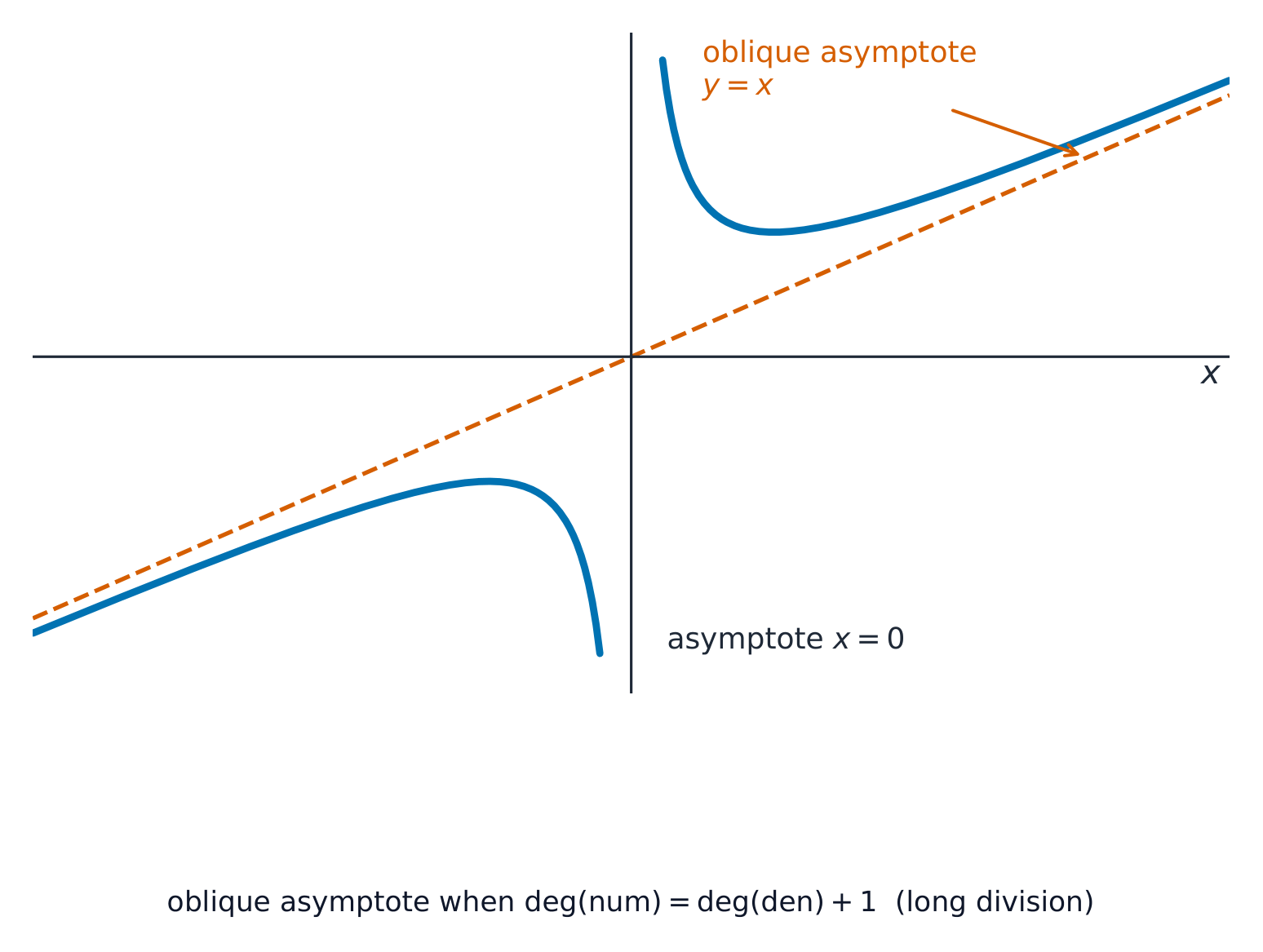
A rational function 有理函数 is a fraction of two polynomials. When the top has degree exactly one higher than the bottom, the graph has an oblique asymptote 斜渐近线 (a slanted line the curve approaches); find it by dividing out. You should also be able to relate the graph of $y = f(x)$ to those of $y^2 = f(x)$, $y = \dfrac{1}{f(x)}$, $y = |f(x)|$ and $y = f(|x|)$. Find the set of values the function can take using the discriminant 判别式, and locate its turning points 驻点.
Worked example. Find the oblique asymptote of $y = \dfrac{x^2 + x + 1}{x + 1}$.
Divide out the fraction: $\dfrac{x^2 + x + 1}{x + 1} = x + \dfrac{1}{x + 1}$. As $x \to \pm\infty$ the remainder $\dfrac{1}{x+1} \to 0$, so the curve approaches the line $y = x$ — the oblique asymptote.
The method of differences 差分法 sums a series by cancelling middle terms: if partial fractions 部分分式 write each term as $f(r) - f(r+1)$, almost everything cancels. From the sum to $n$ terms you can see whether a series is convergent 收敛 and, if so, find its sum to infinity 无穷和.
Worked example. Find $\displaystyle\sum_{r=1}^{n} (2r + 1)$.
$$\sum_{r=1}^{n}(2r + 1) = 2\sum_{r=1}^{n} r + \sum_{r=1}^{n} 1 = 2\cdot\tfrac12 n(n+1) + n = n(n+1) + n = n(n+2).$$
carry out operations of matrix addition, subtraction and multiplication, and recognise the terms zero matrix and identity (or unit) matrix
Including non-square matrices. Matrices will have at most 3 rows and columns.
recall the meaning of the terms singular and non-singular as applied to square matrices and, for $2 \times 2$ and $3 \times 3$ matrices, evaluate determinants and find inverses of non-singular matrices
The notations $\det \mathbf{M}$ for the determinant of a matrix $\mathbf{M}$, and $\mathbf{I}$ for the identity matrix, will be used.
understand and use the result, for non-singular matrices, $(\mathbf{AB})^{-1} = \mathbf{B}^{-1}\mathbf{A}^{-1}$
Extension to the product of more than two matrices may be required.
understand the use of $2 \times 2$ matrices to represent certain geometric transformations in the $x$-$y$ plane, in particular: – understand the relationship between the transformations represented by $\mathbf{A}$ and $\mathbf{A}^{-1}$ – recognise that the matrix product $\mathbf{AB}$ represents the transformation that results from the transformation represented by $\mathbf{B}$ followed by the transformation represented by $\mathbf{A}$ – recall how the area scale factor of a transformation is related to the determinant of the corresponding matrix – find the matrix that represents a given transformation or sequence of transformations
Understanding of the terms rotation, reflection, enlargement, stretch and shear for 2D transformations will be required. Other 2D transformations may be included, but no particular knowledge of them is expected.
understand the meaning of invariant as applied to points and lines in the context of transformations represented by matrices, and solve simple problems involving invariant points and invariant lines.
e.g. to locate the invariant points of the transformation represented by $\begin{pmatrix} 6 & 5 \\ 2 & 3 \end{pmatrix}$, or to find the invariant lines through the origin for $\begin{pmatrix} 4 & -1 \\ 2 & 1 \end{pmatrix}$, or to show that any line with gradient 1 is invariant for $\begin{pmatrix} 2 & 0 \\ 1 & 1 \end{pmatrix}$.
Source: Cambridge International syllabus · 出典: Cambridge International シラバス
English
A matrix moves the plane
A matrix 矩阵 is a rectangular block of numbers. Matrix addition adds entries in matching positions; you can also subtract and multiply matrices (multiplication is row $\times$ column). The zero matrix 零矩阵 has every entry $0$, and the identity matrix 单位矩阵 (or unit matrix) $I$ leaves any matrix unchanged under multiplication.
For a $2\times 2$ matrix $A = \begin{pmatrix} a & b \\ c & d \end{pmatrix}$, the determinant 行列式 is $\det A = ad - bc$. If $\det A \neq 0$ the matrix is non-singular (otherwise it is a singular matrix 奇异矩阵), and the inverse matrix 逆矩阵 is
$$A^{-1} = \frac{1}{ad - bc}\begin{pmatrix} d & -b \\ -c & a \end{pmatrix}.$$
For a product, $(AB)^{-1} = B^{-1}A^{-1}$. A $2\times 2$ matrix can represent a geometric transformation 几何变换 of the plane — a rotation 旋转, reflection 反射, enlargement 放大, stretch 拉伸 or shear 切变: the determinant gives the area scale factor, and a product $AB$ means "do $B$, then $A$". Points or lines that do not move are called invariant points 不变点 and invariant lines 不变直线.
Worked example. Find the inverse of $A = \begin{pmatrix} 3 & 1 \\ 2 & 4 \end{pmatrix}$.
$2\times 2$ 行列 $A = \begin{pmatrix} a & b \\ c & d \end{pmatrix}$ に対して、行列式は $\det A = ad - bc$ である。$\det A \neq 0$ の場合、この行列は非特異行列(そうでなければ特異行列)であり、逆行列は以下の通りである。
$$A^{-1} = \frac{1}{ad - bc}\begin{pmatrix} d & -b \\ -c & a \end{pmatrix}.$$
Change the four entries and watch the unit square map to a new shape. The determinant is the area scale factor. · 4つの要素を変化させ、単位正方形が新たな形状に変換される様子を見る。行列式は面積の拡大率である。
understand the relations between Cartesian and polar coordinates, and convert equations of curves from Cartesian to polar form and vice versa
The convention $r \geqslant 0$ will be used.
sketch simple polar curves, for $0 \leqslant \theta < 2\pi$ or $-\pi < \theta \leqslant \pi$ or a subset of either of these intervals
Detailed plotting of curves will not be required, but sketches will generally be expected to show significant features, such as symmetry, coordinates of intersections with the initial line, the form of the curve at the pole and least/greatest values of $r$.
recall the formula $\frac{1}{2} \int r^2 \mathrm{d}\theta$ for the area of a sector, and use this formula in simple cases.
You should sketch simple polar curves 极坐标曲线, and find the area of a sector with
$$\text{area} = \tfrac12\int r^2\,d\theta.$$
Worked example. Convert the polar equation $r = 4\cos\theta$ to Cartesian form.
Multiply both sides by $r$: $r^2 = 4r\cos\theta$, so $x^2 + y^2 = 4x$. Completing the square gives $(x - 2)^2 + y^2 = 4$, a circle of radius $2$ centred at $(2, 0)$.
Pick a curve and change a. In polar form a point is set by its distance r and angle θ — that draws roses, cardioids and spirals. · 曲線を選択して a を変更する。極座標形式では点は距離 r と角度 θ で指定され、これによりバラ曲線、心形線、螺旋線が描かれる。
use the equation of a plane in any of the forms $ax + by + cz = d$ or $\mathbf{r.n} = p$ or $\mathbf{r} = \mathbf{a} + \lambda\mathbf{b} + \mu\mathbf{c}$ and convert equations of planes from one form to another as necessary in solving problems
recall that the vector product$\mathbf{a} \times \mathbf{b}$ of two vectors can be expressed either as $|\mathbf{a}||\mathbf{b}|\sin\theta\hat{\mathbf{n}}$, where $\hat{\mathbf{n}}$ is a unit vector, or in component form as $(a_2b_3 - a_3b_2)\mathbf{i} + (a_3b_1 - a_1b_3)\mathbf{j} + (a_1b_2 - a_2b_1)\mathbf{k}$
use equations of lines and planes, together with scalar and vector products where appropriate, to solve problems concerning distances, angles and intersections, including: – determining whether a line lies in a plane, is parallel to a plane or intersects a plane, and finding the point of intersection of a line and a plane when it exists – finding the foot of the perpendicular from a point to a plane – finding the angle between a line and a plane, and the angle between two planes – finding an equation for the line of intersection of two planes – calculating the shortest distance between two skew lines – finding an equation for the common perpendicular to two skew lines.
Source: Cambridge International syllabus · 出典: Cambridge International シラバス
English
In three dimensions a plane 平面 can be written as $ax + by + cz = d$, or $\mathbf{r}\cdot\mathbf{n} = p$, or $\mathbf{r} = \mathbf{a} + \lambda\mathbf{b} + \mu\mathbf{c}$. Besides the scalar product, there is the vector product 向量积 of two vectors 向量:
which gives a vector at right angles to both. With scalar and vector products you can find distances, angles, and where lines and planes meet — including the shortest distance between skew lines 异面直线.
Worked example. Find $\mathbf{a}\times\mathbf{b}$ for $\mathbf{a} = \mathbf{i} + \mathbf{j}$ and $\mathbf{b} = \mathbf{j} + \mathbf{k}$.
use the method of mathematical induction to establish a given result
e.g. $\sum_{r=1}^{n} r^4 = \frac{1}{4}n^2(n+1)^2$, $u_n = \frac{1}{2}(1 + 3^{n-1})$ for the sequence given by $u_{n+1} = 3u_n - 1$ and $u_1 = 1$, $\begin{pmatrix} 4 & -1 \\ 6 & -1 \end{pmatrix}^n = \begin{pmatrix} 3 \times 2^n - 2 & 1 - 2^n \\ 3 \times 2^{n+1} - 6 & 3 - 2^{n+1} \end{pmatrix}$, $3^{2n} + 2 \times 5^n - 3$ is divisible by 8.
recognise situations where conjecture based on a limited trial followed by inductive proof is a useful strategy, and carry this out in simple cases.
e.g. find the $n$th derivative of $x e^x$, find $\sum_{r=1}^{n} r \times r!$.
Source: Cambridge International syllabus · 出典: Cambridge International シラバス
English
Induction: the domino proof
Mathematical induction 数学归纳法 proves a result for every positive integer $n$ in two steps:
Base case: show the result is true for $n = 1$.
Inductive step: assume it is true for $n = k$, then prove it for $n = k + 1$.
If both steps work, the result is true for all $n$. Often you first make a conjecture 猜想 (a sensible guess) from a few cases, then confirm it by inductive proof 归纳证明.
Worked example. Prove that $\displaystyle\sum_{r=1}^{n} r = \tfrac12 n(n+1)$.
Base case$n = 1$: the left side is $1$ and the right side is $\tfrac12(1)(2) = 1$. True.
Inductive step: assume $\displaystyle\sum_{r=1}^{k} r = \tfrac12 k(k+1)$. Then
This handout covers Topic 2: Further Pure Mathematics 进阶纯数学 2. It adds hyperbolic functions, eigenvalues, new differentiation and integration, de Moivre's theorem, and methods for differential equations.
日本語
This handout covers Topic 2: Further Pure Mathematics 进阶纯数学 2. It adds hyperbolic functions, eigenvalues, new differentiation and integration, de Moivre's theorem, and methods for differential equations.
2.1
Hyperbolic functions
Syllabus · シラバス
English
Candidates should be able to:
Notes and examples
understand the definitions of the hyperbolic functions$\sinh x$, $\cosh x$, $\tanh x$, $\text{sech } x$, $\text{cosech } x$, $\text{coth } x$ in terms of the exponential function
sketch the graphs of hyperbolic functions
prove and use identities involving hyperbolic functions
e.g. $\cosh^2 x - \sinh^2 x \equiv 1$, $\sinh 2x \equiv 2 \sinh x \cosh x$, and similar results corresponding to the standard trigonometric identities.
understand and use the definitions of the inverse hyperbolic functions and derive and use the logarithmic forms
e.g. $\cosh^2 x - \sinh^2 x \equiv 1$, $\sinh 2x \equiv 2 \sinh x \cosh x$ および標準的な三角関数の恒等式に対応する同様の結果.
逆双曲線関数の定義を理解し利用し、対数形を導出・利用する
Source: Cambridge International syllabus · 出典: Cambridge International シラバス
English
cosh and sinh built from exponentials
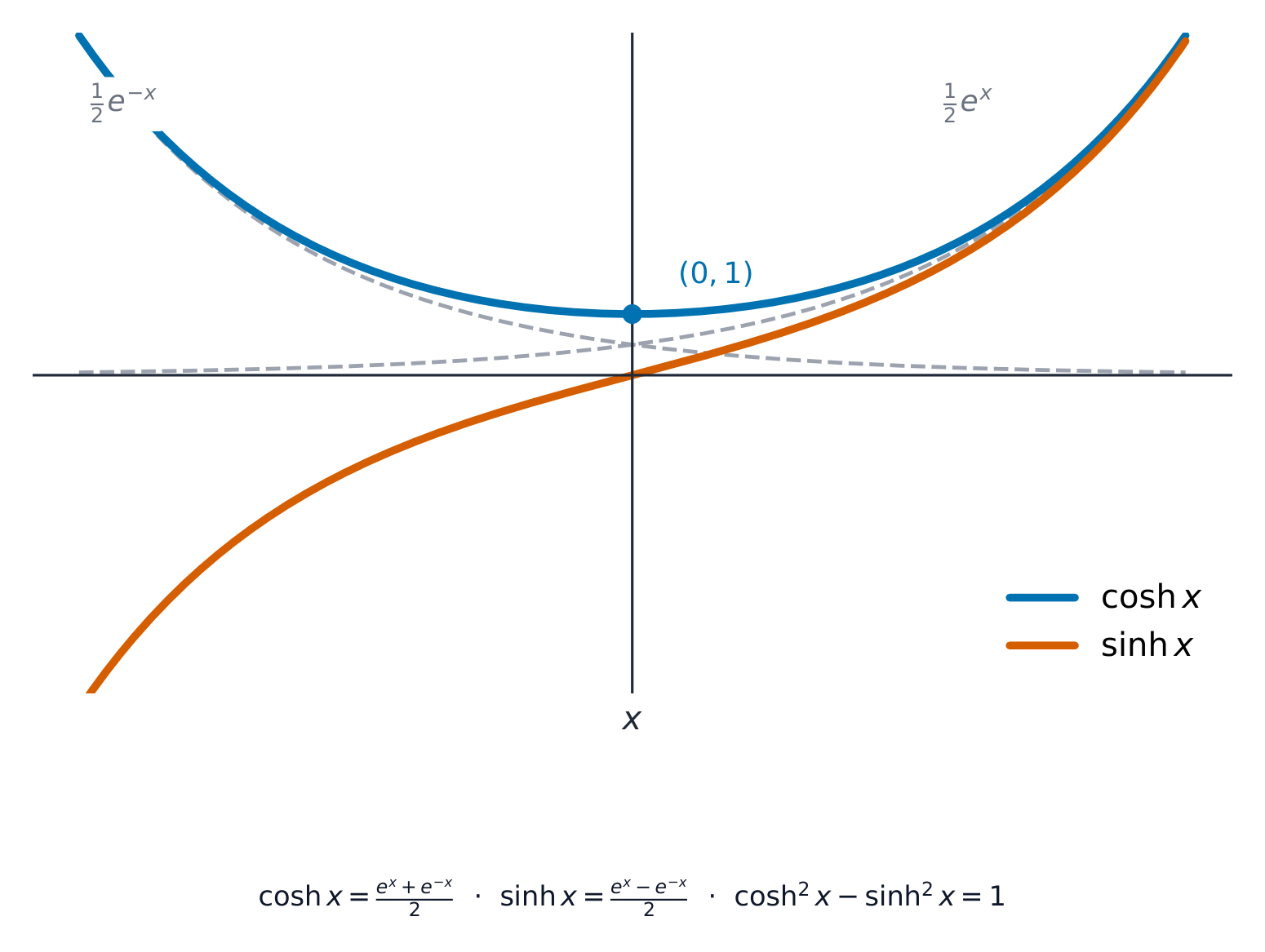
The hyperbolic functions 双曲函数 are built from the exponential function:
$$\cosh x = \frac{e^x + e^{-x}}{2}, \qquad \sinh x = \frac{e^x - e^{-x}}{2}, \qquad \tanh x = \frac{\sinh x}{\cosh x}.$$
They obey identities much like the trigonometric ones, the main one being $\cosh^2 x - \sinh^2 x = 1$. The three reciprocals complete the set: $\operatorname{sech} x = \dfrac{1}{\cosh x}$, $\operatorname{cosech} x = \dfrac{1}{\sinh x}$, and $\coth x = \dfrac{1}{\tanh x} = \dfrac{\cosh x}{\sinh x}$ – all built from $e^x$ too, and worth recognising in integrals and mark schemes. The inverse hyperbolic functions 反双曲函数 have a logarithmic form 对数形式, for example $\sinh^{-1} x = \ln\!\left(x + \sqrt{x^2 + 1}\right)$.
Worked example. Show that $\cosh^2 x - \sinh^2 x = 1$.
cosh and sinh built from exponentialsA hanging cable forms a catenary — the curve of the hyperbolic cosine.
The hyperbolic functions 双曲函数 are built from the exponential function:
$$\cosh x = \frac{e^x + e^{-x}}{2}, \qquad \sinh x = \frac{e^x - e^{-x}}{2}, \qquad \tanh x = \frac{\sinh x}{\cosh x}.$$
$\cosh$ is the average of $e^x$ and $e^{-x}$; $\sinh$ is half their difference.
They obey identities much like the trigonometric ones, the main one being $\cosh^2 x - \sinh^2 x = 1$. The three reciprocals complete the set: $\operatorname{sech} x = \dfrac{1}{\cosh x}$, $\operatorname{cosech} x = \dfrac{1}{\sinh x}$, and $\coth x = \dfrac{1}{\tanh x} = \dfrac{\cosh x}{\sinh x}$ – all built from $e^x$ too, and worth recognising in integrals and mark schemes. The inverse hyperbolic functions 反双曲函数 have a logarithmic form 对数形式, for example $\sinh^{-1} x = \ln\!\left(x + \sqrt{x^2 + 1}\right)$.
Worked example. Show that $\cosh^2 x - \sinh^2 x = 1$.
formulate a problem involving the solution of 3 linear simultaneous equations in 3 unknowns as a problem involving the solution of a matrix equation, or vice versa
understand the cases that may arise concerning the consistency or inconsistency of 3 linear simultaneous equations, relate them to the singularity or otherwise of the corresponding matrix, solve consistent systems, and interpret geometrically in terms of lines and planes
e.g. three planes meeting in a common point, or in a common line, or having no common points.
understand the terms 'characteristic equation', 'eigenvalue' and 'eigenvector', as applied to square matrices
Including use of the definition $\mathbf{Ae} = \lambda \mathbf{e}$ to prove simple properties, e.g. that $\lambda^n$ is an eigenvalue of $\mathbf{A}^n$.
find eigenvalues and eigenvectors of $2 \times 2$ and $3 \times 3$ matrices
Restricted to cases where the eigenvalues are real and distinct.
express a square matrix in the form $\mathbf{QDQ}^{-1}$, where $\mathbf{D}$ is a diagonal matrix of eigenvalues and $\mathbf{Q}$ is a matrix whose columns are eigenvectors, and use this expression
e.g. in calculating powers of $2 \times 2$ or $3 \times 3$ matrices.
use the fact that a square matrix satisfies its own characteristic equation.
e.g. in finding successive powers of a matrix or finding an inverse matrix; restricted to $2 \times 2$ or $3 \times 3$ matrices only.
Source: Cambridge International syllabus · 出典: Cambridge International シラバス
English
A matrix moves the plane
You can write three linear equations in three unknowns as a single matrix equation 矩阵方程$A\mathbf{x} = \mathbf{b}$. If $A$ is non-singular there is one solution; if $A$ is singular the equations are either inconsistent (no solution) or have infinitely many.
For a square matrix $A$, the characteristic equation 特征方程 is $\det(A - \lambda I) = 0$. Its solutions are the eigenvalues 特征值$\lambda$, and for each one the vector $\mathbf{v}$ with $A\mathbf{v} = \lambda\mathbf{v}$ is an eigenvector 特征向量. You can then write $A = QDQ^{-1}$, where $D$ is a diagonal matrix 对角矩阵 of eigenvalues and the columns of $Q$ are the eigenvectors.
Worked example. Find the eigenvalues of $A = \begin{pmatrix} 2 & 1 \\ 1 & 2 \end{pmatrix}$.
So $\lambda = 1$ or $\lambda = 3$. (The eigenvector for $\lambda = 3$ is $\begin{pmatrix} 1 \\ 1 \end{pmatrix}$ and for $\lambda = 1$ is $\begin{pmatrix} 1 \\ -1 \end{pmatrix}$.)
日本語
A matrix moves the plane
You can write three linear equations in three unknowns as a single matrix equation 矩阵方程 $A\mathbf{x} = \mathbf{b}$. If $A$ is non-singular there is one solution; if $A$ is singular the equations are either inconsistent (no solution) or have infinitely many.
For a square matrix $A$, the characteristic equation 特征方程 is $\det(A - \lambda I) = 0$. Its solutions are the eigenvalues 特征值 $\lambda$, and for each one the vector $\mathbf{v}$ with $A\mathbf{v} = \lambda\mathbf{v}$ is an eigenvector 特征向量. You can then write $A = QDQ^{-1}$, where $D$ is a diagonal matrix 对角矩阵 of eigenvalues and the columns of $Q$ are the eigenvectors.
Multiplying an eigenvector by $A$ only stretches it; a general vector is turned to a new direction.
Worked example. Find the eigenvalues of $A = \begin{pmatrix} 2 & 1 \\ 1 & 2 \end{pmatrix}$.
So $\lambda = 1$ or $\lambda = 3$. (The eigenvector for $\lambda = 3$ is $\begin{pmatrix} 1 \\ 1 \end{pmatrix}$ and for $\lambda = 1$ is $\begin{pmatrix} 1 \\ -1 \end{pmatrix}$.)
Explore · 探索
Transformations and the determinant · 変換と行列式
Change the matrix to rotate, stretch or shear the unit square; the determinant shows how area changes. · 行列を変化させて単位正方形を回転、伸縮、せん断する——行列式は面積の変化を示す。
• differentiate hyperbolic functions and differentiate $\sin^{-1}x$, $\cos^{-1}x$, $\sinh^{-1}x$, $\cosh^{-1}x$ and $\tanh^{-1}x$
• obtain an expression for $\frac{\text{d}^2y}{\text{d}x^2}$ in cases where the relation between $x$ and $y$ is defined implicitly or parametrically
• derive and use the first few terms of a Maclaurin's series for a function.
Derivation of a general term is not included, but successive 'implicit' differentiation steps may be required, e.g. for $y = \tan x$ following an initial differentiation rearranged as $y' = 1 + y^2$.
Source: Cambridge International syllabus · 出典: Cambridge International シラバス
English
You can now differentiate the hyperbolic functions and the inverse functions $\sin^{-1}x$, $\tan^{-1}x$, $\sinh^{-1}x$ and so on. You can also find $\dfrac{d^2y}{dx^2}$ for curves given implicitly or parametrically.
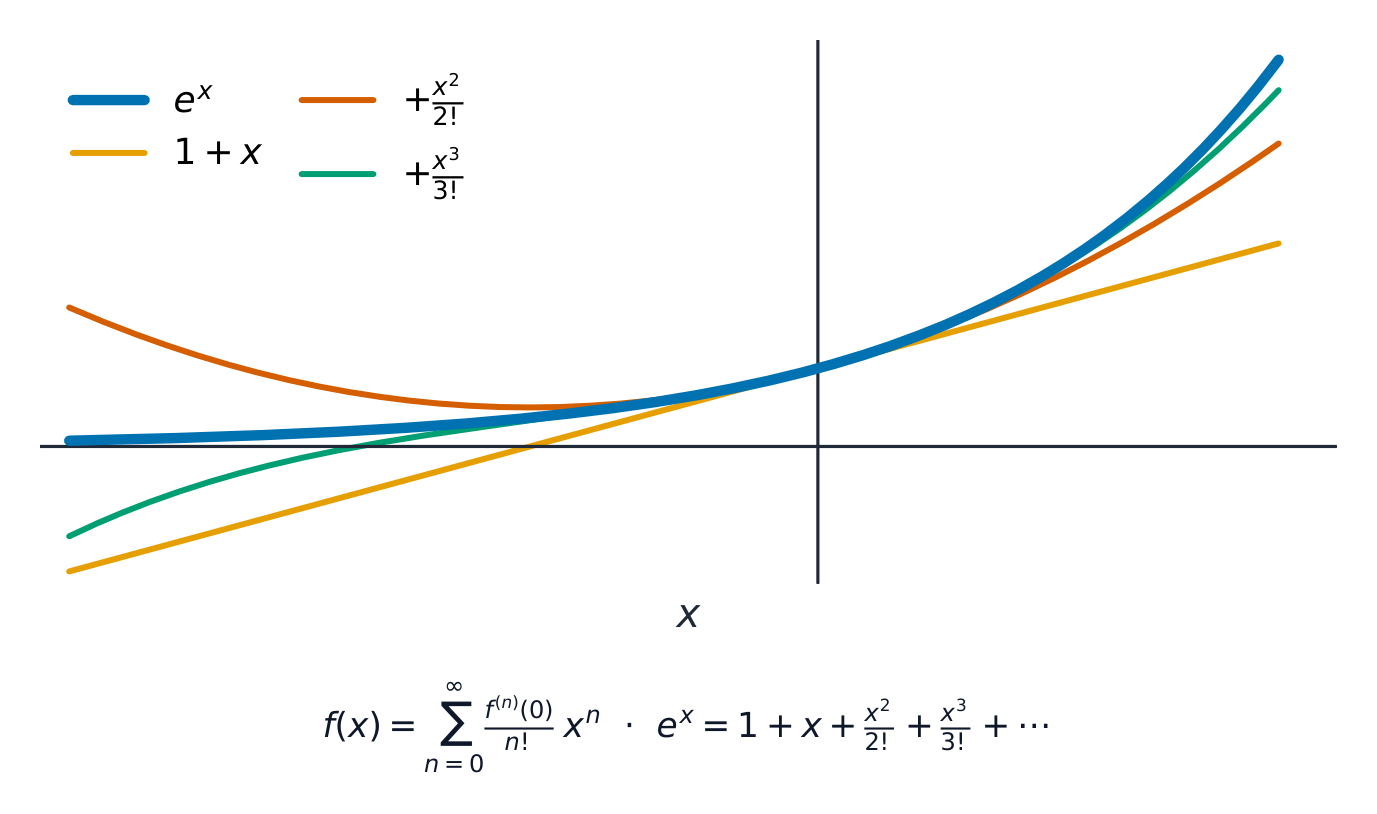
A Maclaurin's series 麦克劳林级数 writes a function as a power series:
For example $e^x = 1 + x + \dfrac{x^2}{2!} + \dfrac{x^3}{3!} + \cdots$
Worked example. Find the Maclaurin series of $f(x) = \ln(1+x)$ up to the term in $x^3$.
$f(0) = 0$; $f'(x) = \dfrac{1}{1+x}$ so $f'(0) = 1$; $f''(x) = \dfrac{-1}{(1+x)^2}$ so $f''(0) = -1$; $f'''(x) = \dfrac{2}{(1+x)^3}$ so $f'''(0) = 2$. Substituting into the series:
$$\ln(1+x) = x - \frac{x^2}{2} + \frac{x^3}{3} - \cdots$$
日本語
You can now differentiate the hyperbolic functions and the inverse functions $\sin^{-1}x$, $\tan^{-1}x$, $\sinh^{-1}x$ and so on. You can also find $\dfrac{d^2y}{dx^2}$ for curves given implicitly or parametrically.
A Maclaurin's series 麦克劳林级数 writes a function as a power series:
For example $e^x = 1 + x + \dfrac{x^2}{2!} + \dfrac{x^3}{3!} + \cdots$Adding more terms makes the polynomial match $e^x$ over a wider stretch around $x=0$.
Worked example. Find the Maclaurin series of $f(x) = \ln(1+x)$ up to the term in $x^3$.
$f(0) = 0$; $f'(x) = \dfrac{1}{1+x}$ so $f'(0) = 1$; $f''(x) = \dfrac{-1}{(1+x)^2}$ so $f''(0) = -1$; $f'''(x) = \dfrac{2}{(1+x)^3}$ so $f'''(0) = 2$. Substituting into the series:
$$\ln(1+x) = x - \frac{x^2}{2} + \frac{x^3}{3} - \cdots$$
Explore · 探索
The gradient at a point · ある点における勾配
gradient = dy/dx · 勾配 = dy/dx
The derivative is the slope of the tangent, however exotic the function. · 導関数とは、どのような複雑な関数であっても、その接線の傾きである。
• integrate hyperbolic functions and recognise integrals of functions of the form $\frac{1}{\sqrt{a^2 - x^2}}$, $\frac{1}{\sqrt{x^2 + a^2}}$ and $\frac{1}{\sqrt{x^2 - a^2}}$, and integrate associated functions using trigonometric substitutions or hyperbolic substitutions as appropriate
Including use of completing the square where necessary, e.g. to integrate $\frac{1}{\sqrt{x^2 + x}}$.
• derive and use reduction formulae for the evaluation of definite integrals
e.g. $\int_0^{\frac{1}{2}\pi} \sin^n x \text{ d}x$, $\int_0^1 \text{e}^{-x}(1-x)^n \text{ d}x$. In harder cases hints may be given, e.g. $\int_0^{\frac{1}{4}\pi} \sec^n x \text{ d}x$ by considering $\frac{\text{d}}{\text{d}x}(\tan x \sec^n x)$.
• understand how the area under a curve may be approximated by areas of rectangles, and use rectangles to estimate or set bounds for the area under a curve or to derive inequalities or limits concerning sums
Questions may involve either rectangles of unit width or rectangles whose width can tend to zero, e.g. $1 + \ln n > \sum_{r=1}^n \frac{1}{r} > \ln(n+1)$, $\sum_{r=1}^n \frac{1}{n}\left(1 + \frac{r}{n}\right)^{-1} \approx \int_0^1 (1+x)^{-1} \text{ d}x$. continued
• use integration to find – arc lengths for curves with equations in Cartesian coordinates, including the use of a parameter, or in polar coordinates – surface areas of revolution about one of the axes for curves with equations in Cartesian coordinates, including the use of a parameter.
Any questions involving integration may require techniques from Cambridge International A Level Mathematics (9709) applied to more difficult cases, e.g. integration by parts for $\int e^x \sin x \mathrm{d}x$, or use of the substitution $t = \tan \frac{1}{2}x$. Surface areas of revolution for curves with equations in polar coordinates will not be required.
積分を含む問題はCambridge International A Level Mathematics (9709)の技術を用いてより難易度の高い場合に適用されることもあり、例:$\int e^x \sin x \mathrm{d}x$に対する部分積分、または置換$t = \tan \frac{1}{2}x$の使用。Cartesian座標以外の回転体表面積は不要。
Source: Cambridge International syllabus · 出典: Cambridge International シラバス
A trigonometric substitution, a hyperbolic substitution, or completing the square 配方法 in the denominator handles related forms. A reduction formula 递推公式 links an integral $I_n$ to $I_{n-1}$, so you can work down step by step. Integration also gives the arc length 弧长 of a curve and the surface area of revolution 旋转曲面面积 when a curve is turned about an axis.
Worked example. Find $\displaystyle\int \frac{1}{\sqrt{4 - x^2}}\,dx$.
Bounding a sum by an integral. Draw rectangles of unit width under, or over, a decreasing curve such as $y=\frac1x$. Each rectangle of height $\frac1r$ is trapped between two integral strips, so summing gives
$$\ln(n+1) < \sum_{r=1}^{n}\frac1r < 1 + \ln n.$$
Shrinking the rectangle width to $\frac1n\to 0$ turns such a sum into a Riemann sum 黎曼和 that equals the integral in the limit, e.g. $\displaystyle\lim_{n\to\infty}\frac1n\sum_{r=1}^{n}f\!\left(\frac{r}{n}\right)=\int_0^1 f(x)\,dx$.
A trigonometric substitution, a hyperbolic substitution, or completing the square 配方法 in the denominator handles related forms. A reduction formula 递推公式 links an integral $I_n$ to $I_{n-1}$, so you can work down step by step. Integration also gives the arc length 弧长 of a curve and the surface area of revolution 旋转曲面面积 when a curve is turned about an axis.
Worked example. Find $\displaystyle\int \frac{1}{\sqrt{4 - x^2}}\,dx$.
Bounding a sum by an integral. Draw rectangles of unit width under, or over, a decreasing curve such as $y=\frac1x$. Each rectangle of height $\frac1r$ is trapped between two integral strips, so summing gives
$$\ln(n+1) < \sum_{r=1}^{n}\frac1r < 1 + \ln n.$$
Shrinking the rectangle width to $\frac1n\to 0$ turns such a sum into a Riemann sum 黎曼和 that equals the integral in the limit, e.g. $\displaystyle\lim_{n\to\infty}\frac1n\sum_{r=1}^{n}f\!\left(\frac{r}{n}\right)=\int_0^1 f(x)\,dx$.
Explore · 探索
The area under the curve · 曲線下の面積
area = ∫ f(x) dx
Every integral measures the area under the curve — drag the limits. · すべての積分は曲線下の面積を測る—— limits をドラッグせよ。
• understand de Moivre’s theorem, for a positive or negative integer exponent, in terms of the geometrical effect of multiplication and division of complex numbers
• prove de Moivre’s theorem for a positive integer exponent
e.g. by induction.
• use de Moivre’s theorem for a positive or negative rational exponent
e.g. expressing $\cos 5\theta$ in terms of $\cos \theta$ or $\tan 5\theta$ in terms of $\tan \theta$.
– to express trigonometrical ratios of multiple angles in terms of powers of trigonometrical ratios of the fundamental angle
e.g. expressing $\sin^6 \theta$ in terms of $\cos 2\theta$, $\cos 4\theta$ and $\cos 6\theta$.
– to express powers of $\sin \theta$ and $\cos \theta$ in terms of multiple angles
– in the summation of series
e.g. using the '$C + \mathrm{i}S$' method to sum series such as $\sum_{r=1}^{n} \binom{n}{r} \sin r\theta$.
It is used to expand $\cos n\theta$ and $\sin n\theta$ in powers, to sum series, and to find the $n$roots of unity 单位根 (the solutions of $z^n = 1$, equally spaced around the unit circle).
Worked example. Use de Moivre's theorem to express $\cos 3\theta$ in terms of $\cos\theta$.
Take the real part of $(\cos\theta + i\sin\theta)^3 = \cos 3\theta + i\sin 3\theta$:
The nth roots of unity form a polygonMultiplying complex numbers: lengths multiply, angles addMultiplying by i is a rotationSelf-similar patterns like Romanesco broccoli arise from iterating functions in the complex plane.
A complex number 复数 in polar form is $z = r(\cos\theta + i\sin\theta)$. De Moivre's theorem 棣莫弗定理 says that for any integer $n$,
It is used to expand $\cos n\theta$ and $\sin n\theta$ in powers, to sum series, and to find the $n$roots of unity 单位根 (the solutions of $z^n = 1$, equally spaced around the unit circle).
The five solutions of $z^5=1$ are equally spaced $72^\circ$ apart on the unit circle.
Worked example. Use de Moivre's theorem to express $\cos 3\theta$ in terms of $\cos\theta$.
Take the real part of $(\cos\theta + i\sin\theta)^3 = \cos 3\theta + i\sin 3\theta$:
Drag the point to explore modulus and argument — the language of complex numbers in polar (modulus–argument) form. · 点をドラッグして絶対値と偏角を探る——複素数の極座標(絶対値–偏角)表示における表現方法である。
• find an integrating factor for a first order linear differential equation, and use an integrating factor to find the general solution
e.g. $\frac{\mathrm{d}y}{\mathrm{d}x} - 2y = x^2$, $x\frac{\mathrm{d}y}{\mathrm{d}x} - y = x^4$, $\frac{\mathrm{d}y}{\mathrm{d}x} + y\coth x = \cosh x$.
• recall the meaning of the terms 'complementary function' and 'particular integral' in the context of linear differential equations, and recall that the general solution is the sum of the complementary function and a particular integral
find the complementary function for a first or second order linear differential equation with constant coefficients
For second order equations, including the cases where the auxiliary equation has distinct real roots, a repeated real root or conjugate complex roots.
recall the form of, and find, a particular integral for a first or second order linear differential equation in the cases where a polynomial or $ae^{bx}$ or $a\cos px + b\sin px$ is a suitable form, and in other simple cases find the appropriate coefficient(s) given a suitable form of particular integral
e.g. evaluate $k$ given that $kx \cos 2x$ is a particular integral of
use a given substitution to reduce a differential equation to a first or second order linear equation with constant coefficients or to a first order equation with separable variables
e.g. the substitution $x = e^t$ to reduce to linear form a differential equation with terms of the form
use initial conditions to find a particular solution to a differential equation, and interpret a solution in terms of a problem modelled by a differential equation.
Source: Cambridge International syllabus · 出典: Cambridge International シラバス
English
For a first order linear equation $\dfrac{dy}{dx} + P(x)\,y = Q(x)$, multiply by the integrating factor 积分因子$\mu = e^{\int P\,dx}$. The left side then becomes $\dfrac{d}{dx}(\mu y)$, so you can integrate directly.
For a linear equation with constant coefficients, the general solution 通解 is the sum of two parts: the complementary function 余函数 (the solution of the equation with the right side set to $0$, found from the auxiliary equation) and a particular integral 特积分 (any one solution of the full equation). Initial conditions then fix the constants to give the particular solution 特解; simpler equations with separable variables 可分离变量 are integrated directly.
Worked example. Solve $\dfrac{dy}{dx} + 2y = e^x$.
The integrating factor is $\mu = e^{\int 2\,dx} = e^{2x}$. Multiplying through gives $\dfrac{d}{dx}\!\left(y\,e^{2x}\right) = e^{3x}$, so
$$y\,e^{2x} = \tfrac13 e^{3x} + C \;\Rightarrow\; y = \tfrac13 e^x + C e^{-2x}.$$
Second order, constant coefficients. For $\dfrac{d^2y}{dx^2}+b\dfrac{dy}{dx}+cy=f(x)$, solve the auxiliary equation 辅助方程$m^2+bm+c=0$. The complementary function depends on its roots:
two distinct real roots $m_1,m_2$: $y=Ae^{m_1x}+Be^{m_2x}$;
Then add a particular integral by trying a form matching $f(x)$ (a polynomial, $ae^{bx}$, or $a\cos px+b\sin px$); if that trial already appears in the complementary function, multiply it by $x$.
Worked example. Solve $\dfrac{d^2y}{dx^2}-4\dfrac{dy}{dx}+4y=0$. The auxiliary equation $m^2-4m+4=(m-2)^2=0$ has a repeated root $m=2$, so $y=(A+Bx)e^{2x}$.
日本語
For a first order linear equation $\dfrac{dy}{dx} + P(x)\,y = Q(x)$, multiply by the integrating factor 积分因子 $\mu = e^{\int P\,dx}$. The left side then becomes $\dfrac{d}{dx}(\mu y)$, so you can integrate directly.
For a linear equation with constant coefficients, the general solution 通解 is the sum of two parts: the complementary function 余函数 (the solution of the equation with the right side set to $0$, found from the auxiliary equation) and a particular integral 特积分 (any one solution of the full equation). Initial conditions then fix the constants to give the particular solution 特解; simpler equations with separable variables 可分离变量 are integrated directly.
A solution curve follows the slope field, staying tangent to the little segments everywhere.
Worked example. Solve $\dfrac{dy}{dx} + 2y = e^x$.
The integrating factor is $\mu = e^{\int 2\,dx} = e^{2x}$. Multiplying through gives $\dfrac{d}{dx}\!\left(y\,e^{2x}\right) = e^{3x}$, so
$$y\,e^{2x} = \tfrac13 e^{3x} + C \;\Rightarrow\; y = \tfrac13 e^x + C e^{-2x}.$$
Second order, constant coefficients. For $\dfrac{d^2y}{dx^2}+b\dfrac{dy}{dx}+cy=f(x)$, solve the auxiliary equation 辅助方程 $m^2+bm+c=0$. The complementary function depends on its roots:
two distinct real roots $m_1,m_2$: $y=Ae^{m_1x}+Be^{m_2x}$;
Then add a particular integral by trying a form matching $f(x)$ (a polynomial, $ae^{bx}$, or $a\cos px+b\sin px$); if that trial already appears in the complementary function, multiply it by $x$.
Worked example. Solve $\dfrac{d^2y}{dx^2}-4\dfrac{dy}{dx}+4y=0$. The auxiliary equation $m^2-4m+4=(m-2)^2=0$ has a repeated root $m=2$, so $y=(A+Bx)e^{2x}$.
Explore · 探索
Differential equations · 微分方程式
dy/dx = a y
The equation sets the slope everywhere; the solution follows those slopes. · 方程式は everywhere で傾きを設定し、解はその傾きに従う。
This handout covers Topic 3: Further Mechanics 进阶力学. It extends mechanics to projectiles, rigid bodies, circular motion, elastic strings, variable forces and collisions. Take $g = 10\ \text{m s}^{-2}$.
日本語
This handout covers Topic 3: Further Mechanics 进阶力学. It extends mechanics to projectiles, rigid bodies, circular motion, elastic strings, variable forces and collisions. Take $g = 10\ \text{m s}^{-2}$.
3.1
Motion of a projectile
Syllabus · シラバス
English
Candidates should be able to:
Notes and examples
• model the motion of a projectile as a particle moving with constant acceleration and understand any limitations of the model
Vector methods are not required
• use horizontal and vertical equations of motion to solve problems on the motion of projectiles, including finding the magnitude and direction of the velocity at a given time or position, the range on a horizontal plane and the greatest height reached
• derive and use the Cartesian equation of the trajectory of a projectile, including problems in which the initial speed and/or angle of projection may be unknown.
Knowledge of the 'bounding parabola' for accessible points is not included.
Source: Cambridge International syllabus · 出典: Cambridge International シラバス
English
Dropped vs thrown: falling together
A projectile 抛射体 moves freely under gravity, so it has constant acceleration 匀加速$g$ downwards and no horizontal acceleration. Treat the horizontal and vertical motions separately. If it is launched at speed $u$ and angle $\alpha$:
$$\text{horizontal: } x = u\cos\alpha\,\cdot t, \qquad \text{vertical: } y = u\sin\alpha\,\cdot t - \tfrac12 g t^2.$$
Eliminating $t$ gives the Cartesian equation 直角坐标方程 of the trajectory 轨迹 (the path), which is a parabola. For a fixed launch speed, all the trajectories lie under a bounding parabola 包络抛物线 (the envelope of reachable points). The range on level ground is $\dfrac{u^2\sin 2\alpha}{g}$ and the greatest height is $\dfrac{u^2\sin^2\alpha}{2g}$.
Worked example. A ball is thrown at $u = 20\ \text{m s}^{-1}$ at $30^\circ$ to the horizontal. Find the range and greatest height.
Dropped vs thrown: falling togetherWater jets follow parabolic paths — the classic projectile motion under gravity.
A projectile 抛射体 moves freely under gravity, so it has constant acceleration 匀加速 $g$ downwards and no horizontal acceleration. Treat the horizontal and vertical motions separately. If it is launched at speed $u$ and angle $\alpha$:
$$\text{horizontal: } x = u\cos\alpha\,\cdot t, \qquad \text{vertical: } y = u\sin\alpha\,\cdot t - \tfrac12 g t^2.$$
Eliminating $t$ gives the Cartesian equation 直角坐标方程 of the trajectory 轨迹 (the path), which is a parabola. For a fixed launch speed, all the trajectories lie under a bounding parabola 包络抛物线 (the envelope of reachable points). The range on level ground is $\dfrac{u^2\sin 2\alpha}{g}$ and the greatest height is $\dfrac{u^2\sin^2\alpha}{2g}$.
The path is a parabola; the launch speed $u$ splits into a steady horizontal part and a vertical part slowed by gravity.
Worked example. A ball is thrown at $u = 20\ \text{m s}^{-1}$ at $30^\circ$ to the horizontal. Find the range and greatest height.
Fire the ball, then change the angle and speed. The horizontal motion is steady while gravity pulls it down — together they trace a parabola. Find the angle for the longest range, and try the Moon. · ボールを打ち上げ、角度と速度を変えてみろ。水平方向の運動は一定で、重力が下向きに引く——これらを合わせると放物線が描かれる。最長飛距離となる角度を探してみよう。月面でも試してみよう。
For questions involving coplanar forces only; understanding of the vector nature of moments is not required.
• use the result that the effect of gravity on a rigid body is equivalent to a single force acting at the centre of mass of the body, and identify the position of the centre of mass of a uniform body using considerations of symmetry
• use given information about the position of the centre of mass of a triangular lamina and other simple shapes
Proofs of results given in the MF19 List of formulae are not required.
• determine the position of the centre of mass of a composite body by considering an equivalent system of particles
Simple cases only, e.g. a uniform L-shaped lamina, or a uniform cone joined at its base to a uniform hemisphere of the same radius.
• use the principle that if a rigid body is in equilibrium under the action of coplanar forces then the vector sum of the forces is zero and the sum of the moments of the forces about any point is zero, and the converse of this
• solve problems involving the equilibrium of a single rigid body under the action of coplanar forces, including those involving toppling or sliding.
Source: Cambridge International syllabus · 出典: Cambridge International シラバス
English
The moment 力矩 of a force about a point is force $\times$ perpendicular distance; it measures turning effect. The weight of a body acts at its centre of mass 质心, which you can find using symmetry 对称 for a uniform flat shape (a lamina 薄片), or by treating a composite body as a set of particles.
A rigid body under coplanar forces 共面力 is in equilibrium 平衡 when two conditions both hold: the vector sum of the forces is zero, and the sum of the moments about any point is zero. A body may also be on the edge of toppling 翻倒 (turning over) or sliding 滑动 (slipping).
Worked example. A uniform beam $AB$ of length $4\ \text{m}$ and weight $100\ \text{N}$ rests on a pivot at $A$. A vertical force $F$ at $B$ keeps it horizontal. Find $F$.
Take moments about $A$ (the weight acts at the centre, $2\ \text{m}$ from $A$):
$$F\times 4 = 100\times 2 \;\Rightarrow\; F = 50\ \text{N}.$$
日本語
The moment 力矩 of a force about a point is force $\times$ perpendicular distance; it measures turning effect. The weight of a body acts at its centre of mass 质心, which you can find using symmetry 对称 for a uniform flat shape (a lamina 薄片), or by treating a composite body as a set of particles.
A rigid body under coplanar forces 共面力 is in equilibrium 平衡 when two conditions both hold: the vector sum of the forces is zero, and the sum of the moments about any point is zero. A body may also be on the edge of toppling 翻倒 (turning over) or sliding 滑动 (slipping).
Taking moments about the pivot $A$ balances the turning effects: $F\times4 = 100\times2$.
Worked example. A uniform beam $AB$ of length $4\ \text{m}$ and weight $100\ \text{N}$ rests on a pivot at $A$. A vertical force $F$ at $B$ keeps it horizontal. Find $F$.
Take moments about $A$ (the weight acts at the centre, $2\ \text{m}$ from $A$):
$$F\times 4 = 100\times 2 \;\Rightarrow\; F = 50\ \text{N}.$$
Explore · 探索
Equilibrium of forces · 力の平衡
resultant = 0 · 合力 = 0
A body is in equilibrium when the forces add tip-to-tail back to zero. · ある物体が 平衡状態 にあるとは、力が 頭から尾へ つなげられたとき結果としてゼロになることを意味する。
understand the concept of angular speed for a particle moving in a circle, and use the relation $v = r\omega$
understand that the acceleration of a particle moving in a circle with constant speed is directed towards the centre of the circle, and use the formulae $r\omega^2$ and $\frac{v^2}{r}$.
Proof of the acceleration formulae is not required.
solve problems which can be modelled by the motion of a particle moving in a horizontal circle with constant speed
solve problems which can be modelled by the motion of a particle in a vertical circle without loss of energy.
Including finding a normal contact force or the tension in a string, locating points at which these are zero, and conditions for complete circular motion.
Source: Cambridge International syllabus · 出典: Cambridge International シラバス
English
For a particle moving in a circle of radius $r$, the angular speed 角速度$\omega$ links to the speed by $v = r\omega$. The acceleration points towards the centre — the centripetal acceleration 向心加速度 — with size
$$a = r\omega^2 = \frac{v^2}{r}.$$
In a horizontal circle 水平圆 the speed is constant — as in a conical pendulum 圆锥摆 (a mass swung on a string). In a vertical circle 竖直圆 use energy conservation, because the speed changes with height; the normal contact force 法向接触力 or string tension provides the centripetal force.
Worked example. A particle moves in a horizontal circle of radius $2\ \text{m}$ with angular speed $3\ \text{rad s}^{-1}$. Find its speed and acceleration.
For a particle moving in a circle of radius $r$, the angular speed 角速度 $\omega$ links to the speed by $v = r\omega$. The acceleration points towards the centre — the centripetal acceleration 向心加速度 — with size
$$a = r\omega^2 = \frac{v^2}{r}.$$
The velocity points along the tangent; the acceleration points inward to the centre.The hammer thrower is a moving diagram of this page. The taut wire pulls the ball toward the centre — that inward pull is the centripetal force — while the ball's velocity points along the tangent. Let go, and with no inward force left the ball flies straight off that tangent
In a horizontal circle 水平圆 the speed is constant — as in a conical pendulum 圆锥摆 (a mass swung on a string). In a vertical circle 竖直圆 use energy conservation, because the speed changes with height; the normal contact force 法向接触力 or string tension provides the centripetal force.
Worked example. A particle moves in a horizontal circle of radius $2\ \text{m}$ with angular speed $3\ \text{rad s}^{-1}$. Find its speed and acceleration.
Circular motion is measured in radians: drag the angle θ and radius r to see the arc swept — angular speed ω turns this into v = rω. · 円周運動はラジアンで測られる:角度 θ と半径 r をドラッグして掃過される弧を見てみよう——角速度 ω はこれを v = rω に変換する。
use Hooke’s law as a model relating the force in an elastic string or spring to the extension or compression, and understand the term modulus of elasticity
use the formula for the elastic potential energy stored in a string or spring
Proof of the formula is not required.
solve problems involving forces due to elastic strings or springs, including those where considerations of work and energy are needed.
e.g. a particle moving horizontally or vertically or on an inclined plane while attached to one or more strings or springs, or a particle attached to an elastic string acting as a 'conical pendulum'.
Source: Cambridge International syllabus · 出典: Cambridge International シラバス
English
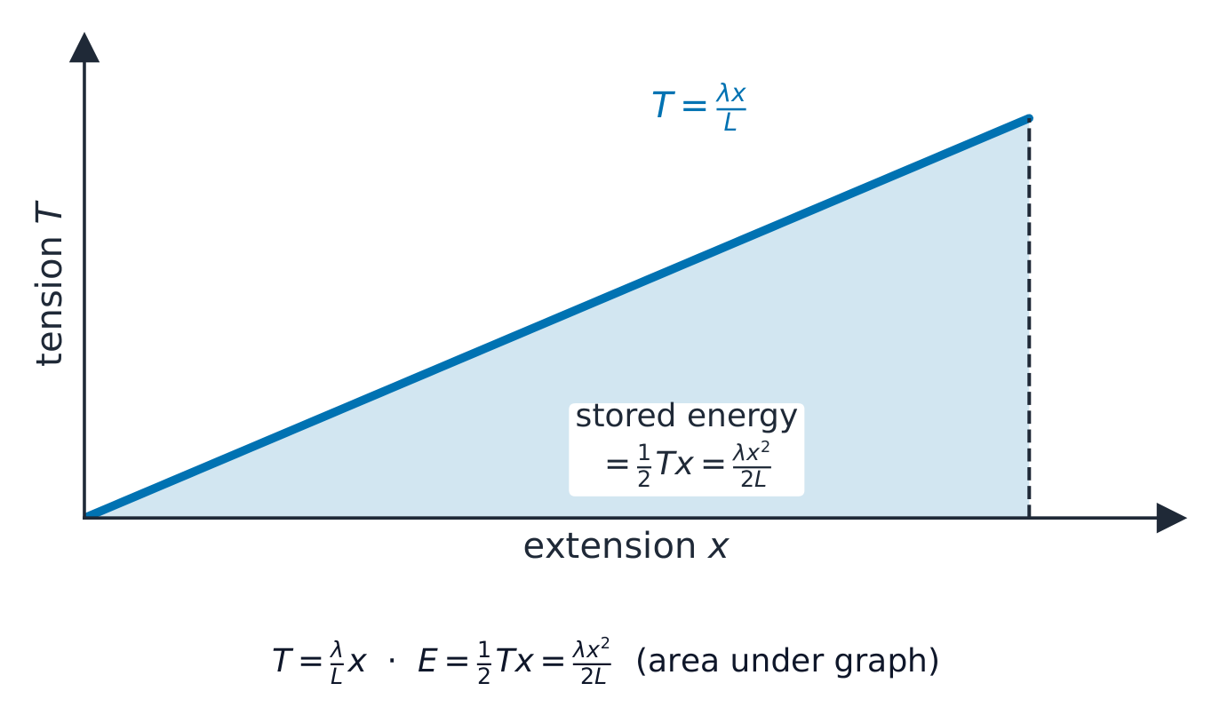
Hooke's law 胡克定律 says the tension in an elastic string or spring is proportional to its extension $x$:
$$T = \frac{\lambda x}{L},$$
where $L$ is the natural length and $\lambda$ is the modulus of elasticity 弹性模量. Stretching stores elastic potential energy 弹性势能:
$$E = \frac{\lambda x^2}{2L}.$$
Worked example. An elastic string of natural length $2\ \text{m}$ and modulus $50\ \text{N}$ is stretched by $0.5\ \text{m}$. Find the tension and the stored energy.
Hooke's law 胡克定律 says the tension in an elastic string or spring is proportional to its extension $x$:
$$T = \frac{\lambda x}{L},$$
where $L$ is the natural length and $\lambda$ is the modulus of elasticity 弹性模量. Stretching stores elastic potential energy 弹性势能:
$$E = \frac{\lambda x^2}{2L}.$$
Tension rises in proportion to extension; the shaded triangle is the stored elastic energy.
Worked example. An elastic string of natural length $2\ \text{m}$ and modulus $50\ \text{N}$ is stretched by $0.5\ \text{m}$. Find the tension and the stored energy.
solve problems which can be modelled as the linear motion of a particle under the action of a variable force, by setting up and solving an appropriate differential equation.
Including use of $v \frac{\mathrm{d}v}{\mathrm{d}x}$ for acceleration, where appropriate. Calculus required is restricted to content from Pure Mathematics 3 in Cambridge International A Level Mathematics (9709). Only differential equations in which the variables are separable are included.
Source: Cambridge International syllabus · 出典: Cambridge International シラバス
English
When the force depends on position $x$, use acceleration in the form $a = v\dfrac{dv}{dx}$, which turns Newton's law into a differential equation 微分方程 relating $v$ and $x$.
Worked example. A particle of mass $8\ \text{kg}$ moves along a line under a variable force 变力 of size $(x^3 + 4x)\ \text{N}$ acting in the direction of motion. When $x = 0$, $v = 1$. Find $v$ in terms of $x$.
Newton's law gives $8v\dfrac{dv}{dx} = x^3 + 4x$. Separating and integrating:
When the force depends on position $x$, use acceleration in the form $a = v\dfrac{dv}{dx}$, which turns Newton's law into a differential equation 微分方程 relating $v$ and $x$.
Use dv/dt when the force depends on time, v dv/dx when it depends on position
Worked example. A particle of mass $8\ \text{kg}$ moves along a line under a variable force 变力 of size $(x^3 + 4x)\ \text{N}$ acting in the direction of motion. When $x = 0$, $v = 1$. Find $v$ in terms of $x$.
Newton's law gives $8v\dfrac{dv}{dx} = x^3 + 4x$. Separating and integrating:
At $x = 0$, $v = 1$ gives $C = 4$, so $4v^2 = \tfrac14 x^4 + 2x^2 + 4 = 4\left(\tfrac{x^2}{4} + 1\right)^2$. Hence $v = \tfrac14 x^2 + 1$.
A position-dependent force becomes a differential equation in v and x
Explore · 探索
Work from a variable force · 可変力からの仕事
W = ∫ F dx
When the force changes, the work done is the area under the force–distance graph. · 力が変化するとき、行われた仕事 は 力–距離グラフの曲線下の面積 である。
recall Newton’s experimental law and the definition of the coefficient of restitution, the property $0 \leqslant e \leqslant 1$, and the meaning of the terms ‘perfectly elastic’ ($e = 1$) and ‘inelastic’ ($e = 0$)
use conservation of linear momentum and/or Newton’s experimental law to solve problems that may be modelled as the direct or oblique impact of two smooth spheres, or the direct or oblique impact of a smooth sphere with a fixed surface.
Source: Cambridge International syllabus · 出典: Cambridge International シラバス
English
In a collision, total linear momentum is conserved — the conservation of linear momentum 动量守恒. The bounciness is measured by Newton's experimental law 牛顿实验定律, which defines the coefficient of restitution 恢复系数$e$:
$$e = \frac{\text{speed of separation}}{\text{speed of approach}}, \qquad 0 \leqslant e \leqslant 1.$$
Here $e = 1$ is perfectly elastic (no energy lost) and $e = 0$ is inelastic (the bodies stay together). In an oblique impact 斜碰撞, resolve the velocities along and perpendicular to the line of impact, applying restitution along it.
Worked example. A sphere $A$ of mass $2\ \text{kg}$ moving at $5\ \text{m s}^{-1}$ hits a stationary sphere $B$ of mass $3\ \text{kg}$, with $e = 0.5$. Find the speeds afterwards.
A Newton's cradle demonstrates conservation of momentum in collisions.
In a collision, total linear momentum is conserved — the conservation of linear momentum 动量守恒. The bounciness is measured by Newton's experimental law 牛顿实验定律, which defines the coefficient of restitution 恢复系数 $e$:
$$e = \frac{\text{speed of separation}}{\text{speed of approach}}, \qquad 0 \leqslant e \leqslant 1.$$
Here $e = 1$ is perfectly elastic (no energy lost) and $e = 0$ is inelastic (the bodies stay together). In an oblique impact 斜碰撞, resolve the velocities along and perpendicular to the line of impact, applying restitution along it.
The coefficient of restitution $e$ compares how fast the bodies separate with how fast they approached.
Worked example. A sphere $A$ of mass $2\ \text{kg}$ moving at $5\ \text{m s}^{-1}$ hits a stationary sphere $B$ of mass $3\ \text{kg}$, with $e = 0.5$. Find the speeds afterwards.
Set each mass and speed, then collide them. Total momentum is conserved — see how the velocities come out. · 各質量と速度を設定して衝突させる。全体的な運動量は保存される——速度がどのように決まるかを確認する。
This handout covers Topic 4: Further Probability & Statistics 进阶概率统计. It adds continuous distributions, small-sample inference, the chi-squared and non-parametric tests, and probability generating functions.
日本語
This handout covers Topic 4: Further Probability & Statistics 进阶概率统计. It adds continuous distributions, small-sample inference, the chi-squared and non-parametric tests, and probability generating functions.
4.1
Continuous random variables
Syllabus · シラバス
Candidates should be able to:
Notes and examples
use a probability density function which may be defined piecewise
use the general result $\text{E}(g(X)) = \int f(x)g(x) \, \mathrm{d}x$ where $f(x)$ is the probability density function of the continuous random variable $X$ and $g(X)$ is a function of $X$
understand and use the relationship between the probability density function (PDF) and the cumulative distribution function (CDF), and use either to evaluate probabilities or percentiles
use cumulative distribution functions (CDFs) of related variables in simple cases.
e.g. given the CDF of a variable $X$, find the CDF of a related variable $Y$, and hence its PDF, e.g. where $Y = X^3$.
Source: Cambridge International syllabus · 出典: Cambridge International シラバス
English
A continuous variable $X$ is described by a probability density function 概率密度函数$f(x)$, which may be defined piecewise. The probability over a range is the area under $f$, and the mean of any function of $X$ is
$$E(g(X)) = \int g(x)\,f(x)\,dx.$$
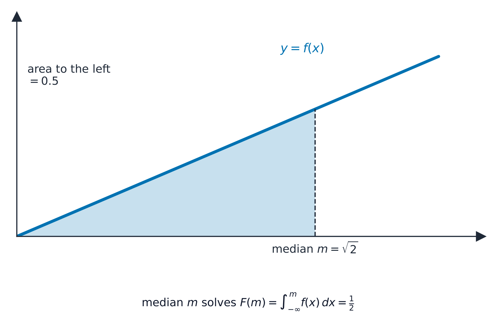
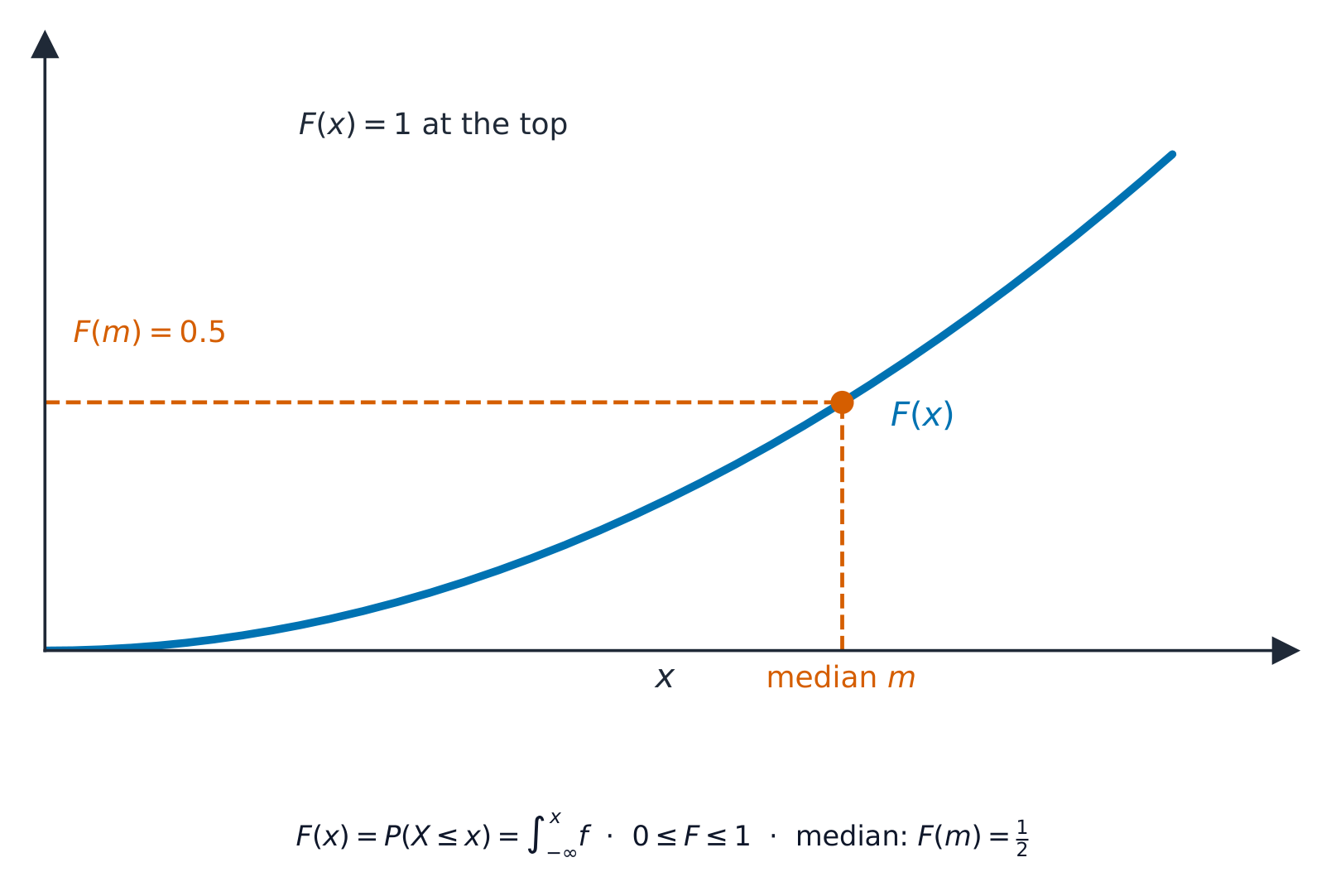
The cumulative distribution function 累积分布函数$F(x) = P(X \leqslant x)$ is the running total: $F(x) = \displaystyle\int_{-\infty}^{x} f(t)\,dt$, and $f(x) = F'(x)$. Use $F$ to find probabilities and percentiles 百分位数 (for example, the median 中位数 solves $F(x) = 0.5$).
Worked example. A variable has $f(x) = \tfrac12 x$ for $0 \leqslant x \leqslant 2$. Find the median.
The cumulative distribution function is $F(x) = \displaystyle\int_0^x \tfrac12 t\,dt = \tfrac14 x^2$. Set $F(m) = 0.5$:
The distribution of a related variable. If $Y=g(X)$, find $Y$'s distribution through its cumulative function. For $Y=X^2$: $F_Y(y)=P(X^2\leqslant y)=P(-\sqrt y\leqslant X\leqslant\sqrt y)=F_X(\sqrt y)-F_X(-\sqrt y)$, then differentiate for $f_Y=F_Y'$. When $g$ is monotonic increasing there is a shortcut, $F_Y(y)=F_X\big(g^{-1}(y)\big)$.
Worked example. With $f_X(x)=\tfrac12 x$ on $[0,2]$ (so $F_X(x)=\tfrac14 x^2$), let $Y=X^2$. For $0\leqslant y\leqslant 4$, $F_Y(y)=F_X(\sqrt y)=\tfrac14 y$, so $f_Y(y)=F_Y'(y)=\tfrac14$ – that is, $Y$ is uniform on $[0,4]$.
日本語
A continuous variable $X$ is described by a probability density function 概率密度函数 $f(x)$, which may be defined piecewise. The probability over a range is the area under $f$, and the mean of any function of $X$ is
$$E(g(X)) = \int g(x)\,f(x)\,dx.$$
The median sits where the area under $f(x)$ to its left is exactly $0.5$.
The cumulative distribution function 累积分布函数 $F(x) = P(X \leqslant x)$ is the running total: $F(x) = \displaystyle\int_{-\infty}^{x} f(t)\,dt$, and $f(x) = F'(x)$. Use $F$ to find probabilities and percentiles 百分位数 (for example, the median 中位数 solves $F(x) = 0.5$).
The cumulative graph $F(x)$ rises from $0$ to $1$; the height $0.5$ is reached at the median.
Worked example. A variable has $f(x) = \tfrac12 x$ for $0 \leqslant x \leqslant 2$. Find the median.
The cumulative distribution function is $F(x) = \displaystyle\int_0^x \tfrac12 t\,dt = \tfrac14 x^2$. Set $F(m) = 0.5$:
The distribution of a related variable. If $Y=g(X)$, find $Y$'s distribution through its cumulative function. For $Y=X^2$: $F_Y(y)=P(X^2\leqslant y)=P(-\sqrt y\leqslant X\leqslant\sqrt y)=F_X(\sqrt y)-F_X(-\sqrt y)$, then differentiate for $f_Y=F_Y'$. When $g$ is monotonic increasing there is a shortcut, $F_Y(y)=F_X\big(g^{-1}(y)\big)$.
Worked example. With $f_X(x)=\tfrac12 x$ on $[0,2]$ (so $F_X(x)=\tfrac14 x^2$), let $Y=X^2$. For $0\leqslant y\leqslant 4$, $F_Y(y)=F_X(\sqrt y)=\tfrac14 y$, so $f_Y(y)=F_Y'(y)=\tfrac14$ – that is, $Y$ is uniform on $[0,4]$.
Explore · 探索
Continuous random variables · 連続型確率変数
P(a < X < b) = ∫ f(x) dx
For a continuous variable, probability is the area under the density curve. · 連続変数において、確率は密度曲線下の面積である。
probability density function/ˌprɒbəˈbɪlɪti ˈdensɪti ˈfʌŋkʃn/
確率密度関数
cumulative distribution function/ˈkjuːmjʊlətɪv ˌdɪstrɪˈbjuːʃn ˈfʌŋkʃn/
累積分布関数
percentiles/pəˈsentaɪlz/
パーセンタイル
median/ˈmiːdiːən/
中央値
4.2
Inference using normal and t-distributions
Syllabus · シラバス
English
Candidates should be able to:
Notes and examples
formulate hypotheses and apply a hypothesis test concerning the population mean using a small sample drawn from a normal population of unknown variance, using a t-test
calculate a pooled estimate of a population variance from two samples
Calculations based on either raw or summarised data may be required.
formulate hypotheses concerning the difference of population means, and apply, as appropriate: - a 2-sample t-test - a paired sample t-test - a test using a normal distribution
The ability to select the test appropriate to the circumstances of a problem is expected.
determine a confidence interval for a population mean, based on a small sample from a normal population with unknown variance, using a t-distribution
determine a confidence interval for a difference of population means, using a t-distribution or a normal distribution, as appropriate.
Source: Cambridge International syllabus · 出典: Cambridge International シラバス
English
When a sample is small and the population variance is unknown, base your hypothesis test 假设检验 on the $t$-distribution instead of the normal. The same idea gives a confidence interval 置信区间 for the mean:
$$\bar{x} \pm t\,\frac{s}{\sqrt{n}},$$
where $t$ comes from the $t$-tables with $n - 1$ degrees of freedom. To compare two populations, use a two-sample (2-sample) or paired-sample$t$-test, after finding a pooled estimate 合并估计 of the shared variance when appropriate.
Worked example. A sample of $n = 10$ has mean $\bar{x} = 50$ and standard deviation $s = 4$. Find a $95\%$ confidence interval for the mean (use $t = 2.262$ for $9$ degrees of freedom).
A Galton board: balls falling through pins pile up into the bell-shaped normal distribution.
When a sample is small and the population variance is unknown, base your hypothesis test 假设检验 on the $t$-distribution instead of the normal. The same idea gives a confidence interval 置信区间 for the mean:
$$\bar{x} \pm t\,\frac{s}{\sqrt{n}},$$
where $t$ comes from the $t$-tables with $n - 1$ degrees of freedom. To compare two populations, use a two-sample (2-sample) or paired-sample$t$-test, after finding a pooled estimate 合并估计 of the shared variance when appropriate.
For a small sample the $t$-distribution is flatter with heavier tails, so its critical values are larger.
Worked example. A sample of $n = 10$ has mean $\bar{x} = 50$ and standard deviation $s = 4$. Find a $95\%$ confidence interval for the mean (use $t = 2.262$ for $9$ degrees of freedom).
Why small samples need t instead of z · 小サンプルで t 分布を使う必要がある理由
With $\sigma$ unknown you use $t$, and $t$ has heavier tails than the normal (drawn dashed behind it) — so its critical values are larger and the interval is wider. At the worked example's $9$ degrees of freedom the widget reads $t^* = 2.262$, exactly the table value used above. Sweep df up and $t$ collapses onto the normal. · 未知の $\sigma$ に対して $t$ を用い、$t$ は正規分布(破線で背後に描く)より尾が太い——そのため臨界値は大きく、区間も広くなる。解例の $9$ 自由度においてウィジェットは $t^* = 2.262$ を読み取り、これは上記で使用した表の値と一致する。df を上げると $t$ は正規分布に収束する。
Explore · 探索
The normal distribution · 正規分布
Shade a tail to find a probability — the basis of confidence intervals and hypothesis tests. · 片側 tail を着色して確率を求める——信頼区間や仮説検定の基礎である。
fit a theoretical distribution, as prescribed by a given hypothesis, to given data
Questions will not involve lengthy calculations.
use a $\chi^2$-test, with the appropriate number of degrees of freedom, to carry out the corresponding goodness of fit analysis
Classes should be combined so that each expected frequency is at least 5.
use a $\chi^2$-test, with the appropriate number of degrees of freedom, for independence in a contingency table.
Yates’ correction is not required. Where appropriate, either rows or columns should be combined so that the expected frequency in each cell is at least 5.
Source: Cambridge International syllabus · 出典: Cambridge International シラバス
English
A $\chi^2$-test (chi-squared test 卡方检验) compares observed counts $O$ with expected counts $E$ from a theoretical distribution 理论分布:
$$\chi^2 = \sum \frac{(O - E)^2}{E}.$$
Compare this with a table value for the right number of degrees of freedom 自由度. Two uses: a goodness of fit 拟合优度 test (does the data follow the proposed model?), and a test for independence 独立性 of two variables in a contingency table 列联表.
Worked example. Four equally likely categories give observed counts $20, 30, 25, 25$ (so each expected count is $25$). Test the fit at the $5\%$ level.
With $4 - 1 = 3$ degrees of freedom the table value is $7.815$. Since $2 < 7.815$, do not reject the model.
日本語
A $\chi^2$-test (chi-squared test 卡方检验) compares observed counts $O$ with expected counts $E$ from a theoretical distribution 理论分布:
$$\chi^2 = \sum \frac{(O - E)^2}{E}.$$
Compare this with a table value for the right number of degrees of freedom 自由度. Two uses: a goodness of fit 拟合优度 test (does the data follow the proposed model?), and a test for independence 独立性 of two variables in a contingency table 列联表.
The test rejects the model when $\chi^2$ exceeds the critical value, landing in the shaded $5\%$ tail.
Worked example. Four equally likely categories give observed counts $20, 30, 25, 25$ (so each expected count is $25$). Test the fit at the $5\%$ level.
With $4 - 1 = 3$ degrees of freedom the table value is $7.815$. Since $2 < 7.815$, do not reject the model.
Explore · 探索
The chi-squared distribution and its 5% tail · カイ二乗分布と5%の右端
The worked example on this page gives $\chi^2 = 2$ with $3$ degrees of freedom against a table value of $7.815$ — the widget reproduces both. Drag df to see why the critical value changes with the number of categories. · このページの worked example は $\chi^2 = 2$ を $3$ の自由度に対して示しており、表の値は $7.815$ です。このウィジェットは両方を再現します。df をドラッグして、カテゴリー数によって臨界値がなぜ変化するかを確認してください。
Explore · 探索
Chi-squared test route · カイ二乗検定の流れ
Follow observed and expected counts to a test decision. · 観測値と期待値に基づき検定の結論を出す。
understand the idea of a non-parametric test and appreciate situations in which such a test might be useful
e.g. when sampling from a population which cannot be assumed to be normally distributed.
understand the basis of the sign test, the Wilcoxon signed-rank test and the Wilcoxon rank-sum test
Including knowledge that Wilcoxon tests are valid only for symmetrical distributions.
use a single-sample sign test and a single-sample Wilcoxon signed-rank test to test a hypothesis concerning a population median
Including the use of normal approximations where appropriate. Questions will not involve tied ranks or observations equal to the population median value being tested.
use a paired-sample sign test, a Wilcoxon matched-pairs signed-rank test and a Wilcoxon rank-sum test, as appropriate, to test for identity of populations.
Including the use of normal approximations where appropriate. Questions will not involve tied ranks or zero‑difference pairs.
Source: Cambridge International syllabus · 出典: Cambridge International シラバス
English
A non-parametric test 非参数检验 makes no assumption that the data is normal, so it is useful when that assumption fails. The basic ones are:
the sign test 符号检验: count how many values fall above and below a proposed median, and test those counts with a binomial model;
the Wilcoxon signed-rank test 威尔科克森符号秩检验 (the matched-pairs test for paired data), which also uses the sizes of the differences, not just their signs;
the Wilcoxon rank-sum test 威尔科克森秩和检验, for comparing two separate samples.
Worked example. Test whether a median is $5$. In a sample of $10$ values (none equal to $5$), $9$ lie above$5$ and $1$ lies below. Test at the $5\%$ level (two-tailed).
Under $H_0$ (median $= 5$) the number above follows $B(10, 0.5)$. The observed result ($9$ above) is extreme, so find $P(X \geq 9) = \binom{10}{9}(0.5)^{10} + (0.5)^{10} = \dfrac{11}{1024} = 0.0107$. For a two-tailed test compare with $\tfrac{1}{2}(5\%) = 0.025$. Since $0.0107 < 0.025$, reject $H_0$: there is evidence the median is not $5$.
日本語
A non-parametric test 非参数检验 makes no assumption that the data is normal, so it is useful when that assumption fails. The basic ones are:
the sign test 符号检验: count how many values fall above and below a proposed median, and test those counts with a binomial model;
the Wilcoxon signed-rank test 威尔科克森符号秩检验 (the matched-pairs test for paired data), which also uses the sizes of the differences, not just their signs;
the Wilcoxon rank-sum test 威尔科克森秩和检验, for comparing two separate samples.
The sign test counts how many values fall above and below the proposed median, then tests those counts with a binomial model
Worked example. Test whether a median is $5$. In a sample of $10$ values (none equal to $5$), $9$ lie above$5$ and $1$ lies below. Test at the $5\%$ level (two-tailed).
Under $H_0$ (median $= 5$) the number above follows $B(10, 0.5)$. The observed result ($9$ above) is extreme, so find $P(X \geq 9) = \binom{10}{9}(0.5)^{10} + (0.5)^{10} = \dfrac{11}{1024} = 0.0107$. For a two-tailed test compare with $\tfrac{1}{2}(5\%) = 0.025$. Since $0.0107 < 0.025$, reject $H_0$: there is evidence the median is not $5$.
Explore · 探索
Non-parametric test chooser · 非参数検定の選び方
Choose the rank-based test that matches the data situation. · データの状況に合う順位検定を選択せよ。
understand the concept of a probability generating function (PGF) and construct and use the PGF for given distributions
Including the discrete uniform, binomial, geometric and Poisson distributions.
use formulae for the mean and variance of a discrete random variable in terms of its PGF, and use these formulae to calculate the mean and variance of a given probability distribution
use the result that the PGF of the sum of independent random variables is the product of the PGFs of those random variables.
Source: Cambridge International syllabus · 出典: Cambridge International シラバス
English
The probability generating function 概率母函数 of a discrete variable $X$ is
$$G(t) = E(t^X) = \sum_x P(X = x)\,t^x.$$
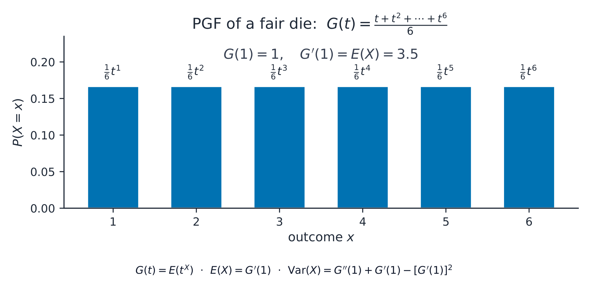
It packs the whole distribution into one function. The mean and variance come from its derivatives at $t = 1$: $E(X) = G'(1)$ and $\mathrm{Var}(X) = G''(1) + G'(1) - \big(G'(1)\big)^2$. Also, the PGF of a sum of independent variables is the product of their PGFs.
Worked example.$X$ has $P(X=0) = 0.5$, $P(X=1) = 0.3$, $P(X=2) = 0.2$. Find $E(X)$ using the PGF.
Here $G(t) = 0.5 + 0.3t + 0.2t^2$, so $G'(t) = 0.3 + 0.4t$ and
$$E(X) = G'(1) = 0.3 + 0.4 = 0.7.$$
日本語
Dice: a starting point for probability and discrete random variables.
The probability generating function 概率母函数 of a discrete variable $X$ is
$$G(t) = E(t^X) = \sum_x P(X = x)\,t^x.$$
It packs the whole distribution into one function. The mean and variance come from its derivatives at $t = 1$: $E(X) = G'(1)$ and $\mathrm{Var}(X) = G''(1) + G'(1) - \big(G'(1)\big)^2$. Also, the PGF of a sum of independent variables is the product of their PGFs.
Worked example.$X$ has $P(X=0) = 0.5$, $P(X=1) = 0.3$, $P(X=2) = 0.2$. Find $E(X)$ using the PGF.
Here $G(t) = 0.5 + 0.3t + 0.2t^2$, so $G'(t) = 0.3 + 0.4t$ and
$$E(X) = G'(1) = 0.3 + 0.4 = 0.7.$$
PGF of a fair die packs equal masses at 1 through 6 into G(t)
Explore · 探索
Probability generating function lab · 確率生成関数の実験
G(x) = p0 + p1 x + p2 x^2 + ...
Change x and see how a PGF stores probabilities in powers of x. · xを変化させ、PGFがxのべき乗で確率をどのように格納するかを確認する。
Type to search notes, lessons, code, vocabulary and past-paper questions across every subject. · すべての科目でノートImplemented、Implemented、コード、語彙、過去問問題を検索するために入力してください。