A-Level Further Mathematics · מתמטיקה מתקדמת A-Level
Tips · טיפים
מתמטיקה נוספת A-Level (9231) יושבת מעל 9709 ומניחה אותה: מתמטיקה נוספת 1 ו-2, מכניקה נוספת, והסתברות וסטטיסטיקה נוספת. היא נלקחת בצדד המתמטיקה, לא במקום שלה, והרכבים שתבצע תלויים בכניסה של בית הספר שלך.
מתמטיקה נוספת מחזיקה את רוב המנגנון החדש — מטריצות וטרנספורמציות ליניאריות, מספרים מרוכבים בצורה קוטבית ואקספוננציאלית, עקומים קוטביים, פונקציות היפרבוליות, משוואות דיפרנציאליות, הוכחה באינדוקציה. זהו תוכן אמיתית חדש, לא גרסאות קשות יותר של תוכן מוכר.
הקושי המציאותי הוא זמן, לא רעיונות. האלגברה ארוכה מספיק כך ששגיאה בשורה שנייה תשרד עד לסוף, ולכן כתוב את השיטה במלואה ובדוק בנקודת האמצע.
This handout covers Topic 1: Further Pure Mathematics 进阶纯数学 1. It adds new algebra, matrices, polar coordinates, more vectors, and proof by induction.
עברית
דף זה מכסה נושא 1: מתמטיקה נקייה נוספת 1. הוא מוסיף אלגברה חדשה, מטריצות, קואורדינטות קוטביות, וקטורים נוספים, והוכחה באינדוקציה.
1.1
Roots of polynomial equations · שורשים של משוואות פולינומיות
Syllabus · סיילבוס
English
Candidates should be able to:
Notes and examples
• recall and use the relations between the roots and coefficients of polynomial equations
e.g. to evaluate symmetric functions of the roots or to solve problems involving unknown coefficients in equations; restricted to equations of degree 2, 3 or 4 only.
• use a substitution to obtain an equation whose roots are related in a simple way to those of the original equation
Substitutions will not be given for the easiest cases, e.g. where the new roots are reciprocals or squares or a simple linear function of the old roots.
עברית
המועמדים אמורים להיות מסוגלים:
הערות לדוגמאות
• להיזכר ולהשתמש בקשרים בין שורשים למקדמים של משוואות פולינומיות
לדוגמה, כדי לחשב פונקציות סימטריות של השורשים או לפתור בעיות המעורבות במקדמים לא ידועים במשוואות; מוגבל למשוואות ממעלה 2, 3 או 4 בלבד.
• להשתמש בהצבה לקבלת משוואה ששורשיה קשורים באופן פשוט לשורשים של המשוואה המקורית
ההצבות לא תינתנה עבור המקרים הקלים ביותר, לדוגמה כאשר השורשים החדשים הם הפוכים, ריבועים או פונקציה ליניארית פשוטה של השורשים הישנים.
Source: Cambridge International syllabus · מקור: הסיילבוס הבינלאומי של קמבריד'ג'
English
For a polynomial equation, the roots 根 are linked to the coefficients 系数. For $ax^2 + bx + c = 0$ with roots $\alpha, \beta$:
Sums like $\sum\alpha$ and $\sum\alpha\beta$ are symmetric functions 对称函数 of the roots (unchanged if the roots are swapped). To find an equation whose roots are changed in a simple way, use a substitution 代换 (for example, put $w = \alpha + 1$).
Worked example. The equation $x^2 - 5x + 6 = 0$ has roots $\alpha, \beta$. Find the equation with roots $\alpha + 1, \beta + 1$.
Here $\alpha + \beta = 5$ and $\alpha\beta = 6$. The new sum is $(\alpha + 1) + (\beta + 1) = 7$, and the new product is $(\alpha + 1)(\beta + 1) = \alpha\beta + \alpha + \beta + 1 = 6 + 5 + 1 = 12$. So the new equation is
$$x^2 - 7x + 12 = 0.$$
עברית
למשוואה פולינומית, ה-שורשים קשורים ל-מקדמים. עבור $ax^2 + bx + c = 0$ עם שורשים $\alpha, \beta$:
סכומים כמו $\sum\alpha$ ו$\sum\alpha\beta$ הם פונקציות סימטריות של השורשים (לא משתנות אם השורשים מוחלפים). כדי למצוא משוואה whose roots are changed in a simple way, use a substitution (for example, put $w = \alpha + 1$).
דוגמה מפורשת. המשוואה $x^2 - 5x + 6 = 0$ יש שורשים $\alpha, \beta$. מצאו את המשוואה עם שורשים $\alpha + 1, \beta + 1$.
הנה $\alpha + \beta = 5$ ו-$\alpha\beta = 6$. הסכום החדש הוא $(\alpha + 1) + (\beta + 1) = 7$, והמכפלה החדשה היא $(\alpha + 1)(\beta + 1) = \alpha\beta + \alpha + \beta + 1 = 6 + 5 + 1 = 12$. לכן המשוואה החדשה היא
$$x^2 - 7x + 12 = 0.$$
Explore · חקור
Roots of a polynomial · שורשים של פולינום
y = ax³ + bx² + cx + d
The roots are where the curve meets the x-axis — their sum and product link to the coefficients. · השורשים הם הנקודות שבהן העקומה חוצה את ציר ה-x — הסכום והמכפלה שלהם קשורים למקדמים.
Further Pure Mathematics/ˈfɜːðə pjʊə ˌmæθɪˈmætɪks/
מתמטיקה נטו נוספת
roots/ruːts/
שורשים
coefficients/ˌkəʊɪˈfɪʃənts/
מקדמים
substitution/ˌsʌbstɪˈtjuːʃn/
החלפה
rational function/ˈræʃənl ˈfʌŋkʃn/
פונקציה רציונלית
1.2
Rational functions and graphs · פונקציות רציונליות וגרפים
Syllabus · סיילבוס
English
Candidates should be able to:
Notes and examples
• sketch graphs of simple rational functions, including the determination of oblique asymptotes, in cases where the degree of the numerator and the denominator are at most 2
Including determination of the set of values taken by the function, e.g. by the use of a discriminant. Detailed plotting of curves will not be required, but sketches will generally be expected to show significant features, such as turning points, asymptotes and intersections with the axes.
• understand and use relationships between the graphs of $y = f(x)$, $y^2 = f(x)$, $y = \frac{1}{f(x)}$, $y = |f(x)|$ and $y = f(|x|)$
Including use of such sketch graphs in the course of solving equations or inequalities.
עברית
המועמדים אמורים להיות מסוגלים:
הערות לדוגמאות
• לערוך גרפים של פונקציות רציונליות פשוטות, כולל קביעת אסימפטוטות אלכסוניות, במקרים שבהם מעלת המונה והמכנה אינם עולים על 2
כולל קביעת קבוצת הערכים הנלקחת על ידי הפונקציה, לדוגמה באמצעות דיסקרימיננטה. ציור מדויק של curves לא יהיה נדרש, אך גרפים טריים יצופו בדרך כלל להציג מאפיינים משמעותיים, כמו נקודות שינוי, אסימפטוטות וחיתוך עם הצירים.
• להבין ולהשתמש בקשרים בין הגרפים של $y = f(x)$, $y^2 = f(x)$, $y = \frac{1}{f(x)}$, $y = |f(x)|$ ו$y = f(|x|)$
כולל השימוש בגרפים טריים אלו בתהליך פתרון משוואות או אי-שוויונות.
Source: Cambridge International syllabus · מקור: הסיילבוס הבינלאומי של קמבריד'ג'
English
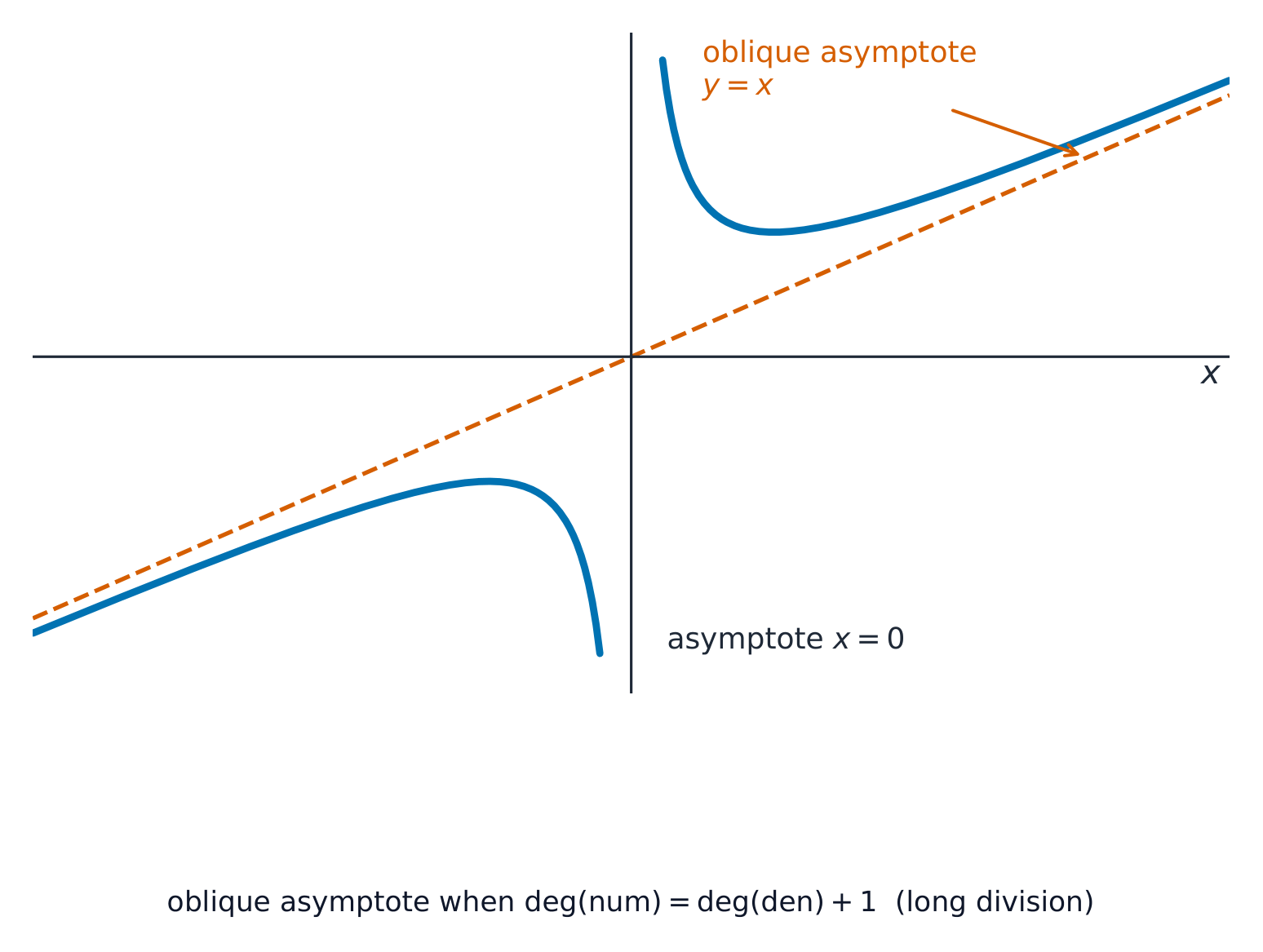
A rational function 有理函数 is a fraction of two polynomials. When the top has degree exactly one higher than the bottom, the graph has an oblique asymptote 斜渐近线 (a slanted line the curve approaches); find it by dividing out. You should also be able to relate the graph of $y = f(x)$ to those of $y^2 = f(x)$, $y = \dfrac{1}{f(x)}$, $y = |f(x)|$ and $y = f(|x|)$. Find the set of values the function can take using the discriminant 判别式, and locate its turning points 驻点.
Worked example. Find the oblique asymptote of $y = \dfrac{x^2 + x + 1}{x + 1}$.
Divide out the fraction: $\dfrac{x^2 + x + 1}{x + 1} = x + \dfrac{1}{x + 1}$. As $x \to \pm\infty$ the remainder $\dfrac{1}{x+1} \to 0$, so the curve approaches the line $y = x$ — the oblique asymptote.
עברית
פונקציה רציונלית היא שבר של שני פולינומים. כאשר דרגת המונה גבוהה ב-1 בדיוק מדרגת המכנה, לגרף יש אסימפטוטה אלכסונית (קו אלכסוני שהעקומה מתקרבת אליו); ניתן למצוא אותה על ידי ביצוע חלוקה. עליך גם להיות מסוגל לקשר את הגרף של $y = f(x)$ לגרפים של $y^2 = f(x)$, $y = \dfrac{1}{f(x)}$, $y = |f(x)|$ ו-$y = f(|x|)$. מצא את קבוצת הערכים שתוכל לקבל מהפונקציה באמצעות הדיסקרימיננטה, ומיקום הנקודות המינוף שלה.
רחוק מהראשית העקומה נדבקת לקו האלכסוני $y=x$; בקרבת $x=0$ היא יורדת לאורך האסימפטוטה האנכית.
דוגמה מפורטת. מצא את האסימפטוטה האלכסונית של $y = \dfrac{x^2 + x + 1}{x + 1}$.
בצע חלוקה לשבר: $\dfrac{x^2 + x + 1}{x + 1} = x + \dfrac{1}{x + 1}$. מכיוון ש-$x \to \pm\infty$ שארית ה$\dfrac{1}{x+1} \to 0$, העקומה מתקרבת לקו $y = x$ — האסימפטוטה האלכסונית.
Explore · חקור
Rational functions · פונקציות רציונליות
y = a/(x − b) + c
A rational function has asymptotes the curve approaches but never touches. · לפונקציה רציונלית יש אסימפטוטות שהעקומה שואפת אליהן אך לעולם אינה נוגעת בהן.
The method of differences 差分法 sums a series by cancelling middle terms: if partial fractions 部分分式 write each term as $f(r) - f(r+1)$, almost everything cancels. From the sum to $n$ terms you can see whether a series is convergent 收敛 and, if so, find its sum to infinity 无穷和.
Worked example. Find $\displaystyle\sum_{r=1}^{n} (2r + 1)$.
$$\sum_{r=1}^{n}(2r + 1) = 2\sum_{r=1}^{n} r + \sum_{r=1}^{n} 1 = 2\cdot\tfrac12 n(n+1) + n = n(n+1) + n = n(n+2).$$
שיטת ההפרשים מחשבת סכום סדרה על ידי ביטול איברים אמצעיים: אם שברים חלקיים כותבים כל איבר כ$f(r) - f(r+1)$, כמעט הכל מתבטל. ממציאת הסכום עד $n$ איברים ניתן לראות האם סדרה מתכנסת, ואם כן, למצוא את סכומה האינסופי.
דוגמה מפורטת. מצא $\displaystyle\sum_{r=1}^{n} (2r + 1)$.
$$\sum_{r=1}^{n}(2r + 1) = 2\sum_{r=1}^{n} r + \sum_{r=1}^{n} 1 = 2\cdot\tfrac12 n(n+1) + n = n(n+1) + n = n(n+2).$$
Explore · חקור
Sequences and their sums · סדרות וסכומיהן
Step through the terms and the running total — the idea behind a series and its sum to n terms. · תנוע לאורך האיברים והסכום הצובר — הרעיון מאחורי סדרה וסכומה ל-n איברים.
carry out operations of matrix addition, subtraction and multiplication, and recognise the terms zero matrix and identity (or unit) matrix
Including non-square matrices. Matrices will have at most 3 rows and columns.
recall the meaning of the terms singular and non-singular as applied to square matrices and, for $2 \times 2$ and $3 \times 3$ matrices, evaluate determinants and find inverses of non-singular matrices
The notations $\det \mathbf{M}$ for the determinant of a matrix $\mathbf{M}$, and $\mathbf{I}$ for the identity matrix, will be used.
understand and use the result, for non-singular matrices, $(\mathbf{AB})^{-1} = \mathbf{B}^{-1}\mathbf{A}^{-1}$
Extension to the product of more than two matrices may be required.
understand the use of $2 \times 2$ matrices to represent certain geometric transformations in the $x$-$y$ plane, in particular: – understand the relationship between the transformations represented by $\mathbf{A}$ and $\mathbf{A}^{-1}$ – recognise that the matrix product $\mathbf{AB}$ represents the transformation that results from the transformation represented by $\mathbf{B}$ followed by the transformation represented by $\mathbf{A}$ – recall how the area scale factor of a transformation is related to the determinant of the corresponding matrix – find the matrix that represents a given transformation or sequence of transformations
Understanding of the terms rotation, reflection, enlargement, stretch and shear for 2D transformations will be required. Other 2D transformations may be included, but no particular knowledge of them is expected.
understand the meaning of invariant as applied to points and lines in the context of transformations represented by matrices, and solve simple problems involving invariant points and invariant lines.
e.g. to locate the invariant points of the transformation represented by $\begin{pmatrix} 6 & 5 \\ 2 & 3 \end{pmatrix}$, or to find the invariant lines through the origin for $\begin{pmatrix} 4 & -1 \\ 2 & 1 \end{pmatrix}$, or to show that any line with gradient 1 is invariant for $\begin{pmatrix} 2 & 0 \\ 1 & 1 \end{pmatrix}$.
עברית
המועמדים אמורים להיות מסוגלים:
הערות לדוגמאות
לבצע פעולות של חיבור, חיסור וכפל מטריצות, ולהכיר את המונחים מטריצת אפס ומטריצת זהות (או יחידה)
כולל מטריצות שאינן רבועיות. המטריצות יהיו בעלות עד 3 שורות ועמודות.
להיזכר במשמעות המונחים סינגולרי ולא-סינגולרי כפי שהם חלים על מטריצות רבועיות, ולעבור על מטריצות $2 \times 2$ ו$3 \times 3$, לחשב קובעים ולמצוא הפוכים של מטריצות לא-סינגולריות
להבין ולהשתמש בתוצאה, עבור מטריצות לא-סינגולריות, $(\mathbf{AB})^{-1} = \mathbf{B}^{-1}\mathbf{A}^{-1}$
הרחבה ל מכפלה של יותר משתי מטריצות עשויה להיות נדרשת.
הבנת השימוש במטריצות $2 \times 2$ כדי לייצג מספר טרנספורמציות גיאומטריות במישור $x$-$y$, ובפרט: – הבנת הקשר בין הטרנספורמציות המיוצגות על ידי $\mathbf{A}$ ו-$\mathbf{A}^{-1}$ – זיהוי כי מכפלת המטריצות $\mathbf{AB}$ מייצגת את הטרנספורמציה הנובעת מהטרנספורמציה המיוצגת על ידי $\mathbf{B}$ שלאחריה נעשית הטרנספורמציה המיוצגת על ידי $\mathbf{A}$ – הזכרת הקשר בין גורם קנה מידה לשטח של טרנספורמציה לבין הדטרמיננטה של המטריצה המתאימה – מציאת המטריצה המייצגת טרנספורמציה נתונה או סדרת טרנספורמציות
דרישה להבנת המונחים סיבוב, השתקפות, הגדלה, מתיחה וזחילה עבור טרנספורמציות 2D. ייתכן שיוכללו טרנספורמציות 2D נוספות, אך אין צורך בידע ספציפי לגביהן.
להבין את המשמעות של בלתי משתנה כפי שהיא חלה על נקודות וקווים בהקשר של המרות המיוצגות על ידי מטריצות, ולפתור בעיות פשוטות המעורבות בנקודות בלתי משתנות וקווים בלתי משתנים.
לדוגמה, למצוא את נקודות השינוי של ההמרה המיוצגת על ידי $\begin{pmatrix} 6 & 5 \\ 2 & 3 \end{pmatrix}$, או למצוא את הקווים הבלתי משתנים העוברים דרך הראשית עבור $\begin{pmatrix} 4 & -1 \\ 2 & 1 \end{pmatrix}$, או להראות כי כל קו עם שיפוע 1 הוא בלתי משתנה עבור $\begin{pmatrix} 2 & 0 \\ 1 & 1 \end{pmatrix}$.
Source: Cambridge International syllabus · מקור: הסיילבוס הבינלאומי של קמבריד'ג'
English
A matrix moves the plane
A matrix 矩阵 is a rectangular block of numbers. Matrix addition adds entries in matching positions; you can also subtract and multiply matrices (multiplication is row $\times$ column). The zero matrix 零矩阵 has every entry $0$, and the identity matrix 单位矩阵 (or unit matrix) $I$ leaves any matrix unchanged under multiplication.
For a $2\times 2$ matrix $A = \begin{pmatrix} a & b \\ c & d \end{pmatrix}$, the determinant 行列式 is $\det A = ad - bc$. If $\det A \neq 0$ the matrix is non-singular (otherwise it is a singular matrix 奇异矩阵), and the inverse matrix 逆矩阵 is
$$A^{-1} = \frac{1}{ad - bc}\begin{pmatrix} d & -b \\ -c & a \end{pmatrix}.$$
For a product, $(AB)^{-1} = B^{-1}A^{-1}$. A $2\times 2$ matrix can represent a geometric transformation 几何变换 of the plane — a rotation 旋转, reflection 反射, enlargement 放大, stretch 拉伸 or shear 切变: the determinant gives the area scale factor, and a product $AB$ means "do $B$, then $A$". Points or lines that do not move are called invariant points 不变点 and invariant lines 不变直线.
Worked example. Find the inverse of $A = \begin{pmatrix} 3 & 1 \\ 2 & 4 \end{pmatrix}$.
מטריצה היא בלוק מלבני של מספרים. חיבור מטריצות מוסיף איברים במיקומים תואמים; ניתן גם לחסר ולכפול מטריצות (כפל הוא שורה $\times$ עמודה). המטריצה הרווחית היא בעלת כל איבר $0$, וה-מטריצה היחידית (או מטריצת היחיד) $I$ משאירה כל מטריצה ללא שינוי תחת כפל.
עבור מטריצה $2\times 2$$A = \begin{pmatrix} a & b \\ c & d \end{pmatrix}$, ה-דטרמיננטה היא $\det A = ad - bc$. אם $\det A \neq 0$ המטריצה היא אי-סינגולרית (אחרת היא מטריצה סינגולרית), וה-מטריצה ההפוכה היא
$$A^{-1} = \frac{1}{ad - bc}\begin{pmatrix} d & -b \\ -c & a \end{pmatrix}.$$
עבור מכפלה, $(AB)^{-1} = B^{-1}A^{-1}$. מטריצה $2\times 2$ יכולה לייצג המרה גיאומטרית של המישור — סיבוב, השתקפות, הגדלה, מתיחה או זחילה: הדטרמיננטה נותנת את גורם הקנה מידה לשטח, ומכפלה $AB$ משמעותה "עשה $B$, אחר כך $A$". נקודות או קווים שלא זזים נקראים נקודות אינבריאנטיות ו-קווים אינבריאנטיים.
המטריצה שולחת את מربع היחיד לפרללוגרם whose שטח הוא הקובעת.
דוגמה מפורטת. מצא את ההפוך של $A = \begin{pmatrix} 3 & 1 \\ 2 & 4 \end{pmatrix}$.
Change the four entries and watch the unit square map to a new shape. The determinant is the area scale factor. · שנה את ארבעת האלמנטים והצפה איך הריבוע היחידה מתמפה לצורה חדשה. הדיטרמיננטה היא גורם הקנה מידה של השטח.
understand the relations between Cartesian and polar coordinates, and convert equations of curves from Cartesian to polar form and vice versa
The convention $r \geqslant 0$ will be used.
sketch simple polar curves, for $0 \leqslant \theta < 2\pi$ or $-\pi < \theta \leqslant \pi$ or a subset of either of these intervals
Detailed plotting of curves will not be required, but sketches will generally be expected to show significant features, such as symmetry, coordinates of intersections with the initial line, the form of the curve at the pole and least/greatest values of $r$.
recall the formula $\frac{1}{2} \int r^2 \mathrm{d}\theta$ for the area of a sector, and use this formula in simple cases.
עברית
המועמדים אמורים להיות מסוגלים:
הערות לדוגמאות
להבין את הקשרים בין קואורדינטות קרטזיות לקואורדינטות קוטביות, ולהמיר משוואות של curves מפורמ קרטזי לקוטבי ולהפוך
הקונבנציה $r \geqslant 0$ תיستخدم.
שרטט עקומות קוטביות פשוטות, עבור $0 \leqslant \theta < 2\pi$ או $-\pi < \theta \leqslant \pi$ או תת-קבוצה מכל אחד מהמרווחים הללו
אינו נדרש ביצוע גרף מדויק של העקומות, אך יצופה שהשרטוט יציג מאפיינים משמעותיים, כגון סימטריה, קואורדינטות החיתוך עם הקו ההתחלתי, צורת העקומה בקוטב וערכים מינימליים/מקסימליים של $r$.
תזכור את הנוסחה $\frac{1}{2} \int r^2 \mathrm{d}\theta$ לשטח של עיגולית, והשתמש בנוסחה זו במקרים פשוטים.
Source: Cambridge International syllabus · מקור: הסיילבוס הבינלאומי של קמבריד'ג'
English
Tracing a polar curve: the cardioid
Polar coordinates 极坐标 give a point by its distance $r$ from the origin and its angle $\theta$. They link to Cartesian coordinates 直角坐标 by
You should sketch simple polar curves 极坐标曲线, and find the area of a sector with
$$\text{area} = \tfrac12\int r^2\,d\theta.$$
Worked example. Convert the polar equation $r = 4\cos\theta$ to Cartesian form.
Multiply both sides by $r$: $r^2 = 4r\cos\theta$, so $x^2 + y^2 = 4x$. Completing the square gives $(x - 2)^2 + y^2 = 4$, a circle of radius $2$ centred at $(2, 0)$.
עברית
שרטוט עקומה קוטבית: הקרדיוידמדרגות ספירליות: ספיירות מתוארות באופן טבעי באמצעות קואורדינטות קוטביות.
קואורדינטות קוטביות נותנות נקודה לפי המרחק $r$ מהראשית והזווית $\theta$. הן מקושרות לקואורדינטות קרטזיות על ידי
קואורדינטות קוטביות $(r,\theta)$ מונחות לקרטזיות על ידי $x=r\cos\theta$ ו-$y=r\sin\theta$.
עליך לשרטט עקומות קוטביות פשוטות, ולמצוא את שטח העיגולון עם
$$\text{area} = \tfrac12\int r^2\,d\theta.$$
הקרדיויד $r=1+\cos\theta$, מצויר ישירות מתוך $r$ כפונקציה של $\theta$.
דוגמה מוצגת. המרה למשוואה קוטבית $r = 4\cos\theta$ לצורה קרטזית.
כפול את שני האגפים ב-$r$: $r^2 = 4r\cos\theta$, ולכן $x^2 + y^2 = 4x$. השלמת מربع נותנת $(x - 2)^2 + y^2 = 4$, מעגל בעל רדיוס $2$ שמרכזו ב-$(2, 0)$.
Explore · חקור
Polar curves · עקומות קוטביות
Pick a curve and change a. In polar form a point is set by its distance r and angle θ — that draws roses, cardioids and spirals. · בחר עקומה ושנה את a. בצורת הקוטב נקודה מוגדרת לפי המרחק r והזווית θ — הדבר יוצר ורדים, קרדיוئידים וספירלות.
use the equation of a plane in any of the forms $ax + by + cz = d$ or $\mathbf{r.n} = p$ or $\mathbf{r} = \mathbf{a} + \lambda\mathbf{b} + \mu\mathbf{c}$ and convert equations of planes from one form to another as necessary in solving problems
recall that the vector product$\mathbf{a} \times \mathbf{b}$ of two vectors can be expressed either as $|\mathbf{a}||\mathbf{b}|\sin\theta\hat{\mathbf{n}}$, where $\hat{\mathbf{n}}$ is a unit vector, or in component form as $(a_2b_3 - a_3b_2)\mathbf{i} + (a_3b_1 - a_1b_3)\mathbf{j} + (a_1b_2 - a_2b_1)\mathbf{k}$
use equations of lines and planes, together with scalar and vector products where appropriate, to solve problems concerning distances, angles and intersections, including: – determining whether a line lies in a plane, is parallel to a plane or intersects a plane, and finding the point of intersection of a line and a plane when it exists – finding the foot of the perpendicular from a point to a plane – finding the angle between a line and a plane, and the angle between two planes – finding an equation for the line of intersection of two planes – calculating the shortest distance between two skew lines – finding an equation for the common perpendicular to two skew lines.
עברית
המועמדים אמורים להיות מסוגלים:
הערות לדוגמאות
השתמש במשוואת מישור בכל אחת מהצורות $ax + by + cz = d$ או $\mathbf{r.n} = p$ או $\mathbf{r} = \mathbf{a} + \lambda\mathbf{b} + \mu\mathbf{c}$ והמיר משוואות מישור מצורה לצורה אחרת בהתאם הנדרש לפתרון בעיות
תזכור כי מכפלת וקטורית$\mathbf{a} \times \mathbf{b}$ של שני וקטורים ניתן לביטוי גם בצורה $|\mathbf{a}||\mathbf{b}|\sin\theta\hat{\mathbf{n}}$, כאשר $\hat{\mathbf{n}}$ הוא וקטור יחיד, או בצורה רכיבים כ$(a_2b_3 - a_3b_2)\mathbf{i} + (a_3b_1 - a_1b_3)\mathbf{j} + (a_1b_2 - a_2b_1)\mathbf{k}$
השתמש במשוואות של קווים ומישורים, יחד עם מכפלות סקאלריות ווקטוריות כפי שמתאים, לפתרון בעיות הקשורות למרחקים, זוויות וחיתוכים, כולל: – קביעת האם קו נמצא במישור, מקביל למישור או חותך מישור, ומציאת נקודת החיתוך בין קו למישור כאשר היא קיימת – מציאת רגל המטרה מנקודה למישור – מציאת הזווית בין קו למישור, ובין שני מישורים – מציאת משוואה לקו החיתוך של שני מישורים – חישוב המרחק הקצר ביותר בין שני קווים אלכסוניים (שלא נחתכים ולא מקבילים) – מציאת משוואה למטרה המשותפת לשני קווים אלכסוניים.
Source: Cambridge International syllabus · מקור: הסיילבוס הבינלאומי של קמבריד'ג'
English
In three dimensions a plane 平面 can be written as $ax + by + cz = d$, or $\mathbf{r}\cdot\mathbf{n} = p$, or $\mathbf{r} = \mathbf{a} + \lambda\mathbf{b} + \mu\mathbf{c}$. Besides the scalar product, there is the vector product 向量积 of two vectors 向量:
which gives a vector at right angles to both. With scalar and vector products you can find distances, angles, and where lines and planes meet — including the shortest distance between skew lines 异面直线.
Worked example. Find $\mathbf{a}\times\mathbf{b}$ for $\mathbf{a} = \mathbf{i} + \mathbf{j}$ and $\mathbf{b} = \mathbf{j} + \mathbf{k}$.
כוחות כמו רוח ומים הם וקטורים — להם גם גודל וגם כיוון.
בשלושה ממדים מישור ניתן לכתוב כ-$ax + by + cz = d$, או כ-$\mathbf{r}\cdot\mathbf{n} = p$, או כ-$\mathbf{r} = \mathbf{a} + \lambda\mathbf{b} + \mu\mathbf{c}$. בנוסף ל מכפלה סקלרית, קיימת גם מכפלה וקטורית של שני וקטורים:
שמניבה וקטור מאונך לשניהם. עם מכפלות סקלריות ווקטוריות ניתן למצוא מרחקים, זוויות, ואת נקודות החיתוך של ישרים ומישורים — כולל המרחק הקצר ביותר בין ישרים סקסיים (שלוויים).
$\mathbf{a}\times\mathbf{b}$ מאונך לשני הוקטורים; אורכו שווה לשטח המקבילית שהם משקיפים.
דוגמה מוצגת. מצאו $\mathbf{a}\times\mathbf{b}$ עבור $\mathbf{a} = \mathbf{i} + \mathbf{j}$ ו$\mathbf{b} = \mathbf{j} + \mathbf{k}$.
זיהוי מצבים שבהם ניחוש המבוסס על ניסיון מוגבל שאחריו הוכחה אינדוקטיבית היא אסטרטגיה שימושית, וביצוע זאת במקרים פשוטים.
לדוגמה: מציאת ה$n$-הנגזרת של $x e^x$, מציאת $\sum_{r=1}^{n} r \times r!$.
Source: Cambridge International syllabus · מקור: הסיילבוס הבינלאומי של קמבריד'ג'
English
Induction: the domino proof
Mathematical induction 数学归纳法 proves a result for every positive integer $n$ in two steps:
Base case: show the result is true for $n = 1$.
Inductive step: assume it is true for $n = k$, then prove it for $n = k + 1$.
If both steps work, the result is true for all $n$. Often you first make a conjecture 猜想 (a sensible guess) from a few cases, then confirm it by inductive proof 归纳证明.
Worked example. Prove that $\displaystyle\sum_{r=1}^{n} r = \tfrac12 n(n+1)$.
Base case$n = 1$: the left side is $1$ and the right side is $\tfrac12(1)(2) = 1$. True.
Inductive step: assume $\displaystyle\sum_{r=1}^{k} r = \tfrac12 k(k+1)$. Then
This is the formula with $n = k + 1$, so by induction it holds for all $n$.
עברית
אינדוקציה: ההוכחה באמצעות קוביות דומינו
אינדוקציה מתמטית מוכיחה תוצאה לכל מספר טבעי חיובי $n$ בשני שלבים:
מקרה בסיס: להראות שהתוצאה נכונה עבור $n = 1$.
שלב אינדוקטיבי: להניח שהיא נכונה עבור $n = k$, ולאחר מכן להוכיחה עבור $n = k + 1$.
אם שני השלבים עובדים, התוצאה נכונה לכל $n$. לעיתים קרובות תחילה מעשים ניחוש (הנחיה הגיונית) מכמה מקרים, ואז מאשרים אותו באמצעות הוכחת אינדוקציה.
האינדוקציה דומה לקוביות דומינו: מקרה הבסיס הופך את הראשונה, והשלב האינדוקטיבי גורם לכל אחת לגרוף את הבאה — כך התוצאה תקפה לכל n
דוגמה מוצגת. הוכיחו כי $\displaystyle\sum_{r=1}^{n} r = \tfrac12 n(n+1)$.
מקרה בסיס$n = 1$: האגף שמאל הוא $1$ והאגף ימין הוא $\tfrac12(1)(2) = 1$. נכון.
שלב אינדוקטיבי: הנחתי $\displaystyle\sum_{r=1}^{k} r = \tfrac12 k(k+1)$. אז
זוהי הנוסחה עם $n = k + 1$, ולכן לפי עקרון האינדוקציה היא מתקיימת לכל $n$.
Explore · חקור
Proof by induction route · מסלול ההוכחה באמצעות אינדוקציה
See induction as a first domino plus a rule that pushes every next case. · תחשבו על אינדוקציה כעל המדומה הראשונה בתור, שאליו מצטרפת כלל הדוחף את כל המקרה הבא.
This handout covers Topic 2: Further Pure Mathematics 进阶纯数学 2. It adds hyperbolic functions, eigenvalues, new differentiation and integration, de Moivre's theorem, and methods for differential equations.
עברית
דף זה מכסה את הנושא 2: מתמטיקה נקייה מתקדמת 2. הוא מוסיף פונקציות היפרבוליות, ערכים עצמיים, נגזרות ואינטגרלים חדשים, משפט דה מואבר ושיטות לפתרון משוואות דיפרנציאליות.
2.1
Hyperbolic functions · פונקציות היפרבוליות
Syllabus · סיילבוס
English
Candidates should be able to:
Notes and examples
understand the definitions of the hyperbolic functions$\sinh x$, $\cosh x$, $\tanh x$, $\text{sech } x$, $\text{cosech } x$, $\text{coth } x$ in terms of the exponential function
sketch the graphs of hyperbolic functions
prove and use identities involving hyperbolic functions
e.g. $\cosh^2 x - \sinh^2 x \equiv 1$, $\sinh 2x \equiv 2 \sinh x \cosh x$, and similar results corresponding to the standard trigonometric identities.
understand and use the definitions of the inverse hyperbolic functions and derive and use the logarithmic forms
לדוגמה: $\cosh^2 x - \sinh^2 x \equiv 1$, $\sinh 2x \equiv 2 \sinh x \cosh x$ ותוצאות דומות המקבילות לזהויות טריגונומטריות סטנדרטיות.
הבנה והשתמשות בהגדרות של פונקציות ההיפרבוליות ההפוכות וגזירה והשתמשות בצורות הלוגריתמיות שלהן
Source: Cambridge International syllabus · מקור: הסיילבוס הבינלאומי של קמבריד'ג'
English
cosh and sinh built from exponentials
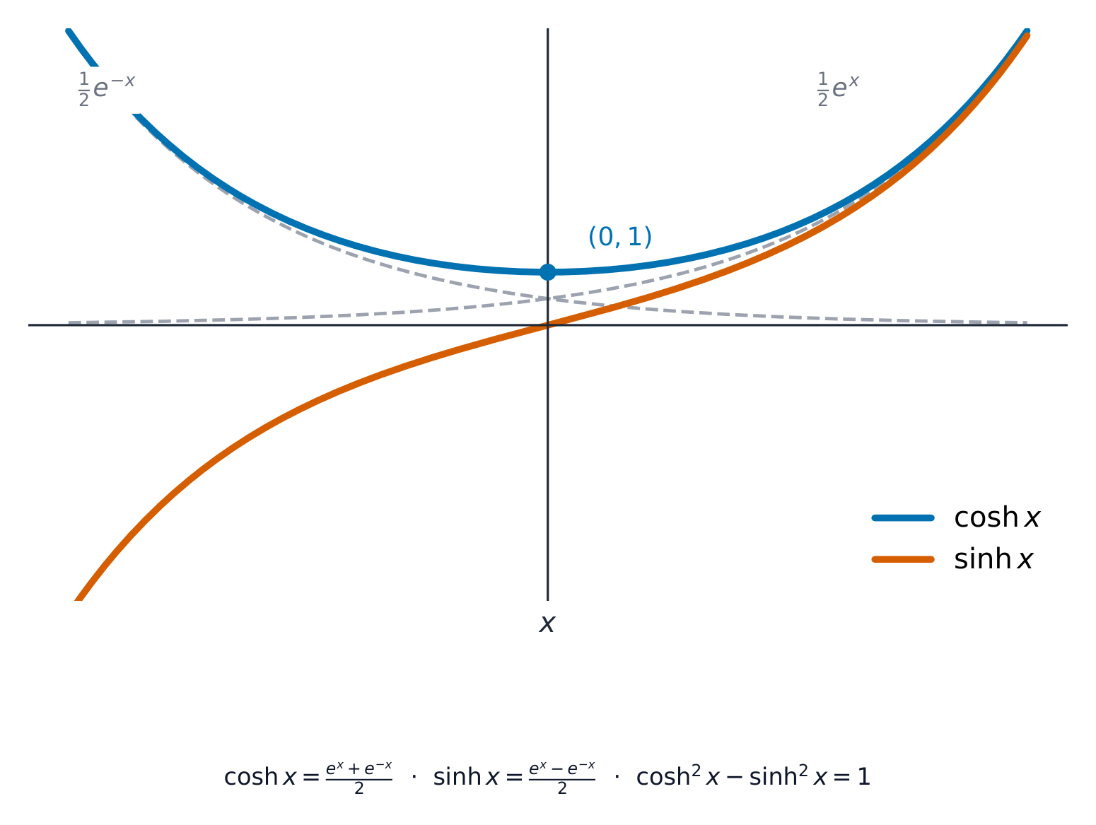
The hyperbolic functions 双曲函数 are built from the exponential function:
$$\cosh x = \frac{e^x + e^{-x}}{2}, \qquad \sinh x = \frac{e^x - e^{-x}}{2}, \qquad \tanh x = \frac{\sinh x}{\cosh x}.$$
They obey identities much like the trigonometric ones, the main one being $\cosh^2 x - \sinh^2 x = 1$. The three reciprocals complete the set: $\operatorname{sech} x = \dfrac{1}{\cosh x}$, $\operatorname{cosech} x = \dfrac{1}{\sinh x}$, and $\coth x = \dfrac{1}{\tanh x} = \dfrac{\cosh x}{\sinh x}$ – all built from $e^x$ too, and worth recognising in integrals and mark schemes. The inverse hyperbolic functions 反双曲函数 have a logarithmic form 对数形式, for example $\sinh^{-1} x = \ln\!\left(x + \sqrt{x^2 + 1}\right)$.
Worked example. Show that $\cosh^2 x - \sinh^2 x = 1$.
$$\cosh x = \frac{e^x + e^{-x}}{2}, \qquad \sinh x = \frac{e^x - e^{-x}}{2}, \qquad \tanh x = \frac{\sinh x}{\cosh x}.$$
$\cosh$ הוא הממוצע של $e^x$ ו-$e^{-x}$; $\sinh$ הוא מחצית ההפרש שלהם.
הן מקיימות זהויות דומות מאוד לאלו הטריגונומטריות, והעיקר בהן הוא $\cosh^2 x - \sinh^2 x = 1$. השלושה הופכים משלים את הסט: $\operatorname{sech} x = \dfrac{1}{\cosh x}$, $\operatorname{cosech} x = \dfrac{1}{\sinh x}$, ו-$\coth x = \dfrac{1}{\tanh x} = \dfrac{\cosh x}{\sinh x}$ – כולם בנויים גם כן מ-$e^x$, וחשוב לזהות אותם באינטגרלים ובמפתח ציונים. הפונקציות ההיפרבוליות ההפוכות להן צורה לוגاریتمית, לדוגמה $\sinh^{-1} x = \ln\!\left(x + \sqrt{x^2 + 1}\right)$.
דוגמה מפורטת. הראו כי $\cosh^2 x - \sinh^2 x = 1$.
cosh is the catenary (a hanging chain) — even, with its minimum at (0, a). · cosh הוא הקטנריה (שרשרת תלויה) — פונקציה זוגית, עם מינימום בנקודה (0, a).
2.2
Matrices · מטריצות
Syllabus · סיילבוס
English
Candidates should be able to:
Notes and examples
formulate a problem involving the solution of 3 linear simultaneous equations in 3 unknowns as a problem involving the solution of a matrix equation, or vice versa
understand the cases that may arise concerning the consistency or inconsistency of 3 linear simultaneous equations, relate them to the singularity or otherwise of the corresponding matrix, solve consistent systems, and interpret geometrically in terms of lines and planes
e.g. three planes meeting in a common point, or in a common line, or having no common points.
understand the terms 'characteristic equation', 'eigenvalue' and 'eigenvector', as applied to square matrices
Including use of the definition $\mathbf{Ae} = \lambda \mathbf{e}$ to prove simple properties, e.g. that $\lambda^n$ is an eigenvalue of $\mathbf{A}^n$.
find eigenvalues and eigenvectors of $2 \times 2$ and $3 \times 3$ matrices
Restricted to cases where the eigenvalues are real and distinct.
express a square matrix in the form $\mathbf{QDQ}^{-1}$, where $\mathbf{D}$ is a diagonal matrix of eigenvalues and $\mathbf{Q}$ is a matrix whose columns are eigenvectors, and use this expression
e.g. in calculating powers of $2 \times 2$ or $3 \times 3$ matrices.
use the fact that a square matrix satisfies its own characteristic equation.
e.g. in finding successive powers of a matrix or finding an inverse matrix; restricted to $2 \times 2$ or $3 \times 3$ matrices only.
עברית
המועמדים אמורים להיות מסוגלים:
הערות לדוגמאות
ניסוח בעיה הכוללת פתרון של 3 משוואות ליניאריות מקבילות ב3 נעלמים כבעיה הכוללת פתרון של משוואת מטריצות, או להפך
הבנת המקרים העלולים להתרחש לגבי התאמה או אי-התאמה של 3 משוואות ליניאריות סמוכות, קשר אותם לסינגולריות או אי-היא של המטריצה המתאימה, פתרון מערכות תואמות, ופרשנות גיאומטרית במונחים של קווים ומישורים
לדוגמה: שלושה מישורים שנפגשים בנקודה משותפת, או בקו משותף, או שאינם משתפים נקודות כלל.
הבנת המונחים 'משוואה אופיינית', 'ערך אופייני' ו'וקטור אופייני', כפי שהם חלים על מטריצות ריבועיות
כולל השימוש בהגדרה $\mathbf{Ae} = \lambda \mathbf{e}$ להוכחת תכונות פשוטות, לדוגמה: כי $\lambda^n$ הוא ערך אופייני של $\mathbf{A}^n$.
מציאת ערכים אופייניים ווקטורים אופייניים של מטריצות $2 \times 2$ ו$3 \times 3$
מוגבל למקרים שבהם הערכים האופייניים הם ממשיים ושונים זה מזה.
ביטוי מטריצה ריבועית בצורה $\mathbf{QDQ}^{-1}$, כאשר $\mathbf{D}$ היא מטריצה אלכסונית של ערכים אופייניים ו$\mathbf{Q}$ היא מטריצה שעמודותיה הן וקטורים אופייניים, והשתמשות בביטוי זה
לדוגמה: בחישוב חזקות של מטריצות $2 \times 2$ או $3 \times 3$.
השתמש בעובדה שמטריצה ריבועית מקיימת את המשוואה האופיינית שלה.
לדוגמה: במציאת חזקות עוקבות של מטריצה או במציאת מטריצה הפוכה; מוגבל רק למטריצות $2 \times 2$ או $3 \times 3$.
Source: Cambridge International syllabus · מקור: הסיילבוס הבינלאומי של קמבריד'ג'
English
A matrix moves the plane
You can write three linear equations in three unknowns as a single matrix equation 矩阵方程$A\mathbf{x} = \mathbf{b}$. If $A$ is non-singular there is one solution; if $A$ is singular the equations are either inconsistent (no solution) or have infinitely many.
For a square matrix $A$, the characteristic equation 特征方程 is $\det(A - \lambda I) = 0$. Its solutions are the eigenvalues 特征值$\lambda$, and for each one the vector $\mathbf{v}$ with $A\mathbf{v} = \lambda\mathbf{v}$ is an eigenvector 特征向量. You can then write $A = QDQ^{-1}$, where $D$ is a diagonal matrix 对角矩阵 of eigenvalues and the columns of $Q$ are the eigenvectors.
Worked example. Find the eigenvalues of $A = \begin{pmatrix} 2 & 1 \\ 1 & 2 \end{pmatrix}$.
So $\lambda = 1$ or $\lambda = 3$. (The eigenvector for $\lambda = 3$ is $\begin{pmatrix} 1 \\ 1 \end{pmatrix}$ and for $\lambda = 1$ is $\begin{pmatrix} 1 \\ -1 \end{pmatrix}$.)
עברית
מטריצה מזיזה את המישור
ניתן לכתוב שלושה משוואות ליניאריות בשלושה נעלמים כמשוואת מטריצה אחת $A\mathbf{x} = \mathbf{b}$. אם $A$ היא לא סינגולרית יש פתרון אחד; אם $A$ היא סינגולרית, המשוואות או אינן תואמות (ללא פתרון) או שיש להן אינסוף פתרונות.
למטריצה ריבועית $A$, המשוואה האופיינית היא $\det(A - \lambda I) = 0$. הפתרונות שלה הם הערכים המיוחדים$\lambda$, ולכל אחד מהם הווקטור $\mathbf{v}$ המקיים $A\mathbf{v} = \lambda\mathbf{v}$ הוא ווקטור מיוחד. לאחר מכן ניתן לכתוב $A = QDQ^{-1}$, כאשר $D$ היא מטריצה אלכסונית של ערכים מיוחדים ועמודות ה-$Q$ הן הווקטורים המיוחדים.
הכפלת ווקטור מיוחד ב-$A$ רק מושכת אותו; וקטור כללי מסתובב לכיוון חדש.
דוגמה מפורטת. מצאו את הערכים המיוחדים של $A = \begin{pmatrix} 2 & 1 \\ 1 & 2 \end{pmatrix}$.
לכן $\lambda = 1$ או $\lambda = 3$. (הווקטור המיוחד עבור $\lambda = 3$ הוא $\begin{pmatrix} 1 \\ 1 \end{pmatrix}$ ועבור $\lambda = 1$ הוא $\begin{pmatrix} 1 \\ -1 \end{pmatrix}$.)
Explore · חקור
Transformations and the determinant · הפיכות והדיטרמיננטה
Change the matrix to rotate, stretch or shear the unit square; the determinant shows how area changes. · שנו את המטריצה כדי לסובב, למתוח או לעוות את הריבוע היחיד; ה-דטרמיננטה מראה כיצד השטח משתנה.
• differentiate hyperbolic functions and differentiate $\sin^{-1}x$, $\cos^{-1}x$, $\sinh^{-1}x$, $\cosh^{-1}x$ and $\tanh^{-1}x$
• obtain an expression for $\frac{\text{d}^2y}{\text{d}x^2}$ in cases where the relation between $x$ and $y$ is defined implicitly or parametrically
• derive and use the first few terms of a Maclaurin's series for a function.
Derivation of a general term is not included, but successive 'implicit' differentiation steps may be required, e.g. for $y = \tan x$ following an initial differentiation rearranged as $y' = 1 + y^2$.
• קבל ביטוי עבור $\frac{\text{d}^2y}{\text{d}x^2}$ במקרים שבהם הקשר בין $x$ ל-$y$ מוגדר אינפלסיטיבית או פרמטרית
• נגזר ושתמש במונחים הראשונים מסדרת מקלורן עבור פונקציה.
הגזרת איבר כללי אינה נכללת, אך ייתכן שיידרשו צעדים עוקבים של גזירה סתומה, לדוגמה עבור $y = \tan x$ לאחר הסדר התחלתי שנעשה על ידי טרנספורמציה כזו: $y' = 1 + y^2$.
Source: Cambridge International syllabus · מקור: הסיילבוס הבינלאומי של קמבריד'ג'
English
You can now differentiate the hyperbolic functions and the inverse functions $\sin^{-1}x$, $\tan^{-1}x$, $\sinh^{-1}x$ and so on. You can also find $\dfrac{d^2y}{dx^2}$ for curves given implicitly or parametrically.
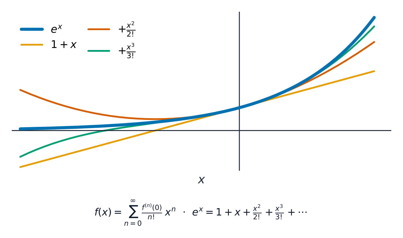
A Maclaurin's series 麦克劳林级数 writes a function as a power series:
For example $e^x = 1 + x + \dfrac{x^2}{2!} + \dfrac{x^3}{3!} + \cdots$
Worked example. Find the Maclaurin series of $f(x) = \ln(1+x)$ up to the term in $x^3$.
$f(0) = 0$; $f'(x) = \dfrac{1}{1+x}$ so $f'(0) = 1$; $f''(x) = \dfrac{-1}{(1+x)^2}$ so $f''(0) = -1$; $f'''(x) = \dfrac{2}{(1+x)^3}$ so $f'''(0) = 2$. Substituting into the series:
$$\ln(1+x) = x - \frac{x^2}{2} + \frac{x^3}{3} - \cdots$$
עברית
עתה ניתן לגזור את הפונקציות ההיפרבוליות ואת הפונקציות ההפוכות $\sin^{-1}x$, $\tan^{-1}x$, $\sinh^{-1}x$ וכדומה. ניתן גם למצוא $\dfrac{d^2y}{dx^2}$ לעקומות נתונות באופן איפלט או פרמטרי.
• integrate hyperbolic functions and recognise integrals of functions of the form $\frac{1}{\sqrt{a^2 - x^2}}$, $\frac{1}{\sqrt{x^2 + a^2}}$ and $\frac{1}{\sqrt{x^2 - a^2}}$, and integrate associated functions using trigonometric substitutions or hyperbolic substitutions as appropriate
Including use of completing the square where necessary, e.g. to integrate $\frac{1}{\sqrt{x^2 + x}}$.
• derive and use reduction formulae for the evaluation of definite integrals
e.g. $\int_0^{\frac{1}{2}\pi} \sin^n x \text{ d}x$, $\int_0^1 \text{e}^{-x}(1-x)^n \text{ d}x$. In harder cases hints may be given, e.g. $\int_0^{\frac{1}{4}\pi} \sec^n x \text{ d}x$ by considering $\frac{\text{d}}{\text{d}x}(\tan x \sec^n x)$.
• understand how the area under a curve may be approximated by areas of rectangles, and use rectangles to estimate or set bounds for the area under a curve or to derive inequalities or limits concerning sums
Questions may involve either rectangles of unit width or rectangles whose width can tend to zero, e.g. $1 + \ln n > \sum_{r=1}^n \frac{1}{r} > \ln(n+1)$, $\sum_{r=1}^n \frac{1}{n}\left(1 + \frac{r}{n}\right)^{-1} \approx \int_0^1 (1+x)^{-1} \text{ d}x$. continued
• use integration to find – arc lengths for curves with equations in Cartesian coordinates, including the use of a parameter, or in polar coordinates – surface areas of revolution about one of the axes for curves with equations in Cartesian coordinates, including the use of a parameter.
Any questions involving integration may require techniques from Cambridge International A Level Mathematics (9709) applied to more difficult cases, e.g. integration by parts for $\int e^x \sin x \mathrm{d}x$, or use of the substitution $t = \tan \frac{1}{2}x$. Surface areas of revolution for curves with equations in polar coordinates will not be required.
עברית
המועמדים אמורים להיות מסוגלים:
הערות לדוגמאות
• אינטגרל פונקציות היפרבוליות והכר זא אינטגרלים של פונקציות מהצורה $\frac{1}{\sqrt{a^2 - x^2}}$, $\frac{1}{\sqrt{x^2 + a^2}}$ ו-$\frac{1}{\sqrt{x^2 - a^2}}$, ואינטגרל פונקציות קשורות באמצעות החלפות טריגונומטריות או החלפות היפרבוליות בהתאם
כולל שימוש ב-השלמת ריבוע כאשר יש צורך, לדוגמה כדי לאינטגרל $\frac{1}{\sqrt{x^2 + x}}$.
• נגזר ושתמש ב-נוסחות הורדה לחישוב אינטגרלים מוגדרים
לדוגמה: $\int_0^{\frac{1}{2}\pi} \sin^n x \text{ d}x$, $\int_0^1 \text{e}^{-x}(1-x)^n \text{ d}x$. במקרים קשים יותר ייתכן שתנתנו רמזים, לדוגמה $\int_0^{\frac{1}{4}\pi} \sec^n x \text{ d}x$ על ידי בחינת $\frac{\text{d}}{\text{d}x}(\tan x \sec^n x)$.
• הבן כיצד ניתן לקרב את השטח תחת עקומה באמצעות שטחי מלבנים, ושתמש במלבנים להערכת שטח תחת עקומה או לקביעת גבולים לשטח זה, או לגזירת אי-שוויונות או גבולות הקשורים לסכומים
ייתכן שהשאלות יכללו מלבנים בעלות רוחב יחיד או מלבנים שרוחבם יכול להתקרב לאפס, לדוגמה: $1 + \ln n > \sum_{r=1}^n \frac{1}{r} > \ln(n+1)$, $\sum_{r=1}^n \frac{1}{n}\left(1 + \frac{r}{n}\right)^{-1} \approx \int_0^1 (1+x)^{-1} \text{ d}x$. המשך...
• השתמש ב-אינטגרציה כדי למצוא – אורכי קשת לעקומות עם משוואות בקואורדינטות קרטזיות, כולל שימוש בפראמטר, או בשטחי פני שטח של סיבוב סביב אחד הצירים לעקומות עם משוואות בקואורדינטות קרטזיות, כולל שימוש בפראמטר.
כל שאלה המכילה אינטגרציה עשויה דורשת טכניקות מתוך Cambridge International A Level Mathematics (9709) המיושמות על מקרים קשים יותר, לדוגמה אינטגרציה בחלקים עבור $\int e^x \sin x \mathrm{d}x$, או שימוש בהחלפה $t = \tan \frac{1}{2}x$. לא יידרש חישוב שטחי פני שטח של סיבוב לעקומות עם משוואות בקואורדינטות קוטביות.
Source: Cambridge International syllabus · מקור: הסיילבוס הבינלאומי של קמבריד'ג'
A trigonometric substitution, a hyperbolic substitution, or completing the square 配方法 in the denominator handles related forms. A reduction formula 递推公式 links an integral $I_n$ to $I_{n-1}$, so you can work down step by step. Integration also gives the arc length 弧长 of a curve and the surface area of revolution 旋转曲面面积 when a curve is turned about an axis.
Worked example. Find $\displaystyle\int \frac{1}{\sqrt{4 - x^2}}\,dx$.
Bounding a sum by an integral. Draw rectangles of unit width under, or over, a decreasing curve such as $y=\frac1x$. Each rectangle of height $\frac1r$ is trapped between two integral strips, so summing gives
$$\ln(n+1) < \sum_{r=1}^{n}\frac1r < 1 + \ln n.$$
Shrinking the rectangle width to $\frac1n\to 0$ turns such a sum into a Riemann sum 黎曼和 that equals the integral in the limit, e.g. $\displaystyle\lim_{n\to\infty}\frac1n\sum_{r=1}^{n}f\!\left(\frac{r}{n}\right)=\int_0^1 f(x)\,dx$.
הצבה טריגונומטרית, הצבה היפרבולית או השלמה לריבוע במכנה מטפלים בצורות הקשורות. נוסחת הפחתה מקשרת אינטגרל $I_n$ ל$I_{n-1}$, כך שניתן לחשב צעד אחר צעד. אינטגרציה מספקת גם את אורך הקשת של עקומה ואת שטח המשטח הנוצר מהיפוך עקומה סביב ציר.
דוגמה מפורטת. מצא $\displaystyle\int \frac{1}{\sqrt{4 - x^2}}\,dx$.
גבול לסכום באמצעות אינטגרל. שרטטו מלבנים בעובי יחיד מתחת או מעל עקומה יורדת כמו $y=\frac1x$. כל מלבן בגובה $\frac1r$ כלוא בין שתי רצועות אינטגרל, ולכן הסכום נותן
$$\ln(n+1) < \sum_{r=1}^{n}\frac1r < 1 + \ln n.$$
צמצום עובי המלבן ל$\frac1n\to 0$ הופך סכום זה לסכום רימן השווה לאינטגרל בגבול, לדוגמה $\displaystyle\lim_{n\to\infty}\frac1n\sum_{r=1}^{n}f\!\left(\frac{r}{n}\right)=\int_0^1 f(x)\,dx$.
Explore · חקור
The area under the curve · השטח תחת העקומה
area = ∫ f(x) dx · שטח = ∫ f(x) dx
Every integral measures the area under the curve — drag the limits. · כל אינטגרל מודד את השטח תחת העקומה — גרור את הגבולות.
• understand de Moivre’s theorem, for a positive or negative integer exponent, in terms of the geometrical effect of multiplication and division of complex numbers
• prove de Moivre’s theorem for a positive integer exponent
e.g. by induction.
• use de Moivre’s theorem for a positive or negative rational exponent
e.g. expressing $\cos 5\theta$ in terms of $\cos \theta$ or $\tan 5\theta$ in terms of $\tan \theta$.
– to express trigonometrical ratios of multiple angles in terms of powers of trigonometrical ratios of the fundamental angle
e.g. expressing $\sin^6 \theta$ in terms of $\cos 2\theta$, $\cos 4\theta$ and $\cos 6\theta$.
– to express powers of $\sin \theta$ and $\cos \theta$ in terms of multiple angles
– in the summation of series
e.g. using the '$C + \mathrm{i}S$' method to sum series such as $\sum_{r=1}^{n} \binom{n}{r} \sin r\theta$.
– in finding and using the $n$th roots of unity.
עברית
המועמדים אמורים להיות מסוגלים:
הערות לדוגמאות
• הבן את משפט דה מואבר, עבור מעריך שלם חיובי או שלילי, במובן ההשפעה הגיאומטרית של הכפלה וחילוק מספרים מרוכבים
• הוכח את משפט דה מואבר עבור מעריך שלם חיובי
לדוגמה: באמצעות אינדוקציה.
• השתמש ב-משפט דה מואבר עבור מעריך רציונלי חיובי או שלילי
לדוגמה: הביע $\cos 5\theta$ באמצעות $\cos \theta$ או $\tan 5\theta$ באמצעות $\tan \theta$.
– ביטוי היחסים הטריגונומטריים של זוויות כפולות באמצעות חזקות של היחסים הטריגונומטריים של הזווית היסודית
לדוגמה: ביטוי $\sin^6 \theta$ באמצעות $\cos 2\theta$, $\cos 4\theta$ ו-$\cos 6\theta$.
– כדי לבטא חזקות של $\sin \theta$ ו-$\cos \theta$ באמצעות זוויות כפולות
– בסכום סדרות
לדוגמה: שיטת ה-'$C + \mathrm{i}S$' לסכום סדרות כמו $\sum_{r=1}^{n} \binom{n}{r} \sin r\theta$.
– במציאה ובשימוש ב-שורשים ה-$n$ של היחידה.
Source: Cambridge International syllabus · מקור: הסיילבוס הבינלאומי של קמבריד'ג'
English
The nth roots of unity form a polygonMultiplying complex numbers: lengths multiply, angles addMultiplying by i is a rotation
A complex number 复数 in polar form is $z = r(\cos\theta + i\sin\theta)$. De Moivre's theorem 棣莫弗定理 says that for any integer $n$,
It is used to expand $\cos n\theta$ and $\sin n\theta$ in powers, to sum series, and to find the $n$roots of unity 单位根 (the solutions of $z^n = 1$, equally spaced around the unit circle).
Worked example. Use de Moivre's theorem to express $\cos 3\theta$ in terms of $\cos\theta$.
Take the real part of $(\cos\theta + i\sin\theta)^3 = \cos 3\theta + i\sin 3\theta$:
השורשים ה-n-יים של היחידות יוצרים רבועוןהכפלת מספרים מרוכבים: האורכים מכפילים, הזוויות מחברותהכפלה ב-i היא סיבובתבניות סמי-דומות כמו כרוב רומנסקו נוצרות על ידי איטרציה של פונקציות במישור המרוכב.
מספר מרוכב בצורה קוטבית הוא $z = r(\cos\theta + i\sin\theta)$. משפט דה מואבר אומר כי לכל מספר שלם $n$,
הוא משמש לפיתוח $\cos n\theta$ ו$\sin n\theta$ בחזקות, לסכום סדרות ולמציאת ה$n$שורשי היחידה (פתרונות המשוואה $z^n = 1$, המפוזרים באופן שווה סביב מעגל היחידה).
חמישת הפתרונות של $z^5=1$ מפוזרים באופן שווה במרחק $72^\circ$ זה מזה על מעגל היחידה.
דוגמה מופתרת. השתמש במשפט דה מואבר כדי לבטא את $\cos 3\theta$ באמצעות $\cos\theta$.
לקח את החלק הממשי של $(\cos\theta + i\sin\theta)^3 = \cos 3\theta + i\sin 3\theta$:
Drag the point to explore modulus and argument — the language of complex numbers in polar (modulus–argument) form. · גרור את הנקודה לחקר המודולוס והארגומנט — לשון המספרים המרוכבים בצורת קוטבית (מודולוס–ארגומנט).
• find an integrating factor for a first order linear differential equation, and use an integrating factor to find the general solution
e.g. $\frac{\mathrm{d}y}{\mathrm{d}x} - 2y = x^2$, $x\frac{\mathrm{d}y}{\mathrm{d}x} - y = x^4$, $\frac{\mathrm{d}y}{\mathrm{d}x} + y\coth x = \cosh x$.
• recall the meaning of the terms 'complementary function' and 'particular integral' in the context of linear differential equations, and recall that the general solution is the sum of the complementary function and a particular integral
find the complementary function for a first or second order linear differential equation with constant coefficients
For second order equations, including the cases where the auxiliary equation has distinct real roots, a repeated real root or conjugate complex roots.
recall the form of, and find, a particular integral for a first or second order linear differential equation in the cases where a polynomial or $ae^{bx}$ or $a\cos px + b\sin px$ is a suitable form, and in other simple cases find the appropriate coefficient(s) given a suitable form of particular integral
e.g. evaluate $k$ given that $kx \cos 2x$ is a particular integral of
use a given substitution to reduce a differential equation to a first or second order linear equation with constant coefficients or to a first order equation with separable variables
e.g. the substitution $x = e^t$ to reduce to linear form a differential equation with terms of the form
use initial conditions to find a particular solution to a differential equation, and interpret a solution in terms of a problem modelled by a differential equation.
עברית
המועמדים אמורים להיות מסוגלים:
הערות לדוגמאות
• מציאת גורם אינטגרציה למשוואה דיפרנציאלית ליניארית מסדר ראשון, ושימוש בגורם זה למציאת הפתרון הכללי
לדוגמה: $\frac{\mathrm{d}y}{\mathrm{d}x} - 2y = x^2$, $x\frac{\mathrm{d}y}{\mathrm{d}x} - y = x^4$, $\frac{\mathrm{d}y}{\mathrm{d}x} + y\coth x = \cosh x$.
• לשחזר את משמעות המונחים פונקציה משלימה ו-אינטגרל פרטי בהקשר של משוואות דיפרנציאליות ליניאריות, ולשחזר שהפתרון הכללי הוא סכום הפונקציה המשלימה והאינטגרל הפרטי
למצוא את הפונקציה המשלימה עבור משוואה דיפרנציאלית ליניארית מסדר ראשון או שני עם מקדמים קבועים
עבור משוואות מסדר שני, כולל המקרים שבהם למשוואה העזרית יש שורשים מציאיים נפרדים, שורש מציאית כפולה או שורשים מרוכבים זוגיים.
הזכרת הצורה ולמציאת אינטגרל פרטי למשוואה דיפרנציאלית ליניארית מסדר ראשון או שני במקרים שבהם פולינום או $ae^{bx}$ או $a\cos px + b\sin px$ הם צורות מתאימות, ובמקרים פשוטים אחרים מציאת המקדם(ים) המתאימים בהינתן צורה מתאימה לאינטגרל פרטי
לדוגמה: חישוב $k$ בהינתן ש-$kx \cos 2x$ הוא אינטגרל פרטי של
להשתמש בתנאי התחלה כדי למצוא פתרון פרטי למשוואה דיפרנציאלית, ולפרש פתרון בהקשר של דגם בעיה המודל על ידי משוואה דיפרנציאלית.
Source: Cambridge International syllabus · מקור: הסיילבוס הבינלאומי של קמבריד'ג'
English
For a first order linear equation $\dfrac{dy}{dx} + P(x)\,y = Q(x)$, multiply by the integrating factor 积分因子$\mu = e^{\int P\,dx}$. The left side then becomes $\dfrac{d}{dx}(\mu y)$, so you can integrate directly.
For a linear equation with constant coefficients, the general solution 通解 is the sum of two parts: the complementary function 余函数 (the solution of the equation with the right side set to $0$, found from the auxiliary equation) and a particular integral 特积分 (any one solution of the full equation). Initial conditions then fix the constants to give the particular solution 特解; simpler equations with separable variables 可分离变量 are integrated directly.
Worked example. Solve $\dfrac{dy}{dx} + 2y = e^x$.
The integrating factor is $\mu = e^{\int 2\,dx} = e^{2x}$. Multiplying through gives $\dfrac{d}{dx}\!\left(y\,e^{2x}\right) = e^{3x}$, so
$$y\,e^{2x} = \tfrac13 e^{3x} + C \;\Rightarrow\; y = \tfrac13 e^x + C e^{-2x}.$$
Second order, constant coefficients. For $\dfrac{d^2y}{dx^2}+b\dfrac{dy}{dx}+cy=f(x)$, solve the auxiliary equation 辅助方程$m^2+bm+c=0$. The complementary function depends on its roots:
two distinct real roots $m_1,m_2$: $y=Ae^{m_1x}+Be^{m_2x}$;
Then add a particular integral by trying a form matching $f(x)$ (a polynomial, $ae^{bx}$, or $a\cos px+b\sin px$); if that trial already appears in the complementary function, multiply it by $x$.
Worked example. Solve $\dfrac{d^2y}{dx^2}-4\dfrac{dy}{dx}+4y=0$. The auxiliary equation $m^2-4m+4=(m-2)^2=0$ has a repeated root $m=2$, so $y=(A+Bx)e^{2x}$.
עברית
עבור משוואה ליניארית מסדר ראשון $\dfrac{dy}{dx} + P(x)\,y = Q(x)$, כפל ב-גורם האינטגרציה$\mu = e^{\int P\,dx}$. צד שמאל יהפוך אז ל$\dfrac{d}{dx}(\mu y)$, כך שתוכל לאינטגרל ישירות.
עבור משוואה ליניארית עם מקדמים קבועים, הפתרון הכללי הוא סכום של שני חלקים: הפונקציה המשלימה (הפתרון למשוואה כאשר הצד ימני מוגדר כ$0$, שנמצא מהמשוואה העזר) והאינטגרל פרטי (כל פתרון אחד של המשוואה המלאה). תנאי התחלה קובעים את הקבועים ומניבים את הפתרון הפרטי; משוואות פשוטות יותר עם משתנים ניתנים להפרדה אינטגרלות ישירות.
עקומת פתרון עוברת לאורך שדה השיפוע, נשארת מגעת למקטעים הקטנים בכל מקום.
דוגמה מופתרת. פתור את $\dfrac{dy}{dx} + 2y = e^x$.
גורם האינטגרציה הוא $\mu = e^{\int 2\,dx} = e^{2x}$. הכפלה במונה מניבה $\dfrac{d}{dx}\!\left(y\,e^{2x}\right) = e^{3x}$, ולכן
$$y\,e^{2x} = \tfrac13 e^{3x} + C \;\Rightarrow\; y = \tfrac13 e^x + C e^{-2x}.$$
דרגה שנייה, מקדמים קבועים. עבור $\dfrac{d^2y}{dx^2}+b\dfrac{dy}{dx}+cy=f(x)$, פתור את המשוואה העזרית$m^2+bm+c=0$. הפונקציה המשלימה תלויה בשורשים שלה:
שני שורשים ממשיים שונים $m_1,m_2$: $y=Ae^{m_1x}+Be^{m_2x}$;
לאחר מכן הוסף אינטגרל פרטי על ידי ניסיון צורה התואמת את $f(x)$ (פולינום, $ae^{bx}$ או $a\cos px+b\sin px$); אם צורה זו מופיעה כבר בפונקציה המשלימה, כפול אותה ב$x$.
דוגמה מופתרת. פתור את $\dfrac{d^2y}{dx^2}-4\dfrac{dy}{dx}+4y=0$. המשוואה העזר $m^2-4m+4=(m-2)^2=0$ היא בעלת שורש כפול $m=2$, ולכן $y=(A+Bx)e^{2x}$.
Explore · חקור
Differential equations · משוואות דיפרנציאליות
dy/dx = a y
The equation sets the slope everywhere; the solution follows those slopes. · המשוואה קובעת את השיפוע בכל מקום; הפתרון עוקב אחר שיפועים אלו.
This handout covers Topic 3: Further Mechanics 进阶力学. It extends mechanics to projectiles, rigid bodies, circular motion, elastic strings, variable forces and collisions. Take $g = 10\ \text{m s}^{-2}$.
עברית
עמוד זה עוסק בנושא 3: מכניקה נוספת. הוא הרחיב את המכניקה לירי רב-כיווני, גוף קשיח, תנועה מעגלית, חוטים אלסטיים, כוחות משתנים והתנגשויות. לקחת $g = 10\ \text{m s}^{-2}$.
3.1
Motion of a projectile · תנועת ירי רב-כיווני
Syllabus · סיילבוס
English
Candidates should be able to:
Notes and examples
• model the motion of a projectile as a particle moving with constant acceleration and understand any limitations of the model
Vector methods are not required
• use horizontal and vertical equations of motion to solve problems on the motion of projectiles, including finding the magnitude and direction of the velocity at a given time or position, the range on a horizontal plane and the greatest height reached
• derive and use the Cartesian equation of the trajectory of a projectile, including problems in which the initial speed and/or angle of projection may be unknown.
Knowledge of the 'bounding parabola' for accessible points is not included.
עברית
המועמדים אמורים להיות מסוגלים:
הערות לדוגמאות
• לדגם את תנועת גוף טס כחלקיק הנע באיץ קבוע ולהבין כל הגבלות הדגם
שיטות וקטוריות אינן נדרשות
• להשתמש במשוואות התנועה האופקיות והאנכיות לפתרון בעיות הקשורות בתנועת גופי טוס, כולל מציאת הגודל והכיוון של המהירות בזמן או מיקום נתונים, הטווח במישור אופקי וגובהו המקסימלי של הגוף
• להסיק ולהשתמש במשוואה הקרטזית של מסלול הגוף הטס, כולל בעיות שבהן המהירות ההתחלתית ו/או זווית השיגור עשויות להיות לא ידועות.
ידע ב'פרבולת החסם' עבור נקודות נגישות אינו כלול.
Source: Cambridge International syllabus · מקור: הסיילבוס הבינלאומי של קמבריד'ג'
English
Dropped vs thrown: falling together
A projectile 抛射体 moves freely under gravity, so it has constant acceleration 匀加速$g$ downwards and no horizontal acceleration. Treat the horizontal and vertical motions separately. If it is launched at speed $u$ and angle $\alpha$:
$$\text{horizontal: } x = u\cos\alpha\,\cdot t, \qquad \text{vertical: } y = u\sin\alpha\,\cdot t - \tfrac12 g t^2.$$
Eliminating $t$ gives the Cartesian equation 直角坐标方程 of the trajectory 轨迹 (the path), which is a parabola. For a fixed launch speed, all the trajectories lie under a bounding parabola 包络抛物线 (the envelope of reachable points). The range on level ground is $\dfrac{u^2\sin 2\alpha}{g}$ and the greatest height is $\dfrac{u^2\sin^2\alpha}{2g}$.
Worked example. A ball is thrown at $u = 20\ \text{m s}^{-1}$ at $30^\circ$ to the horizontal. Find the range and greatest height.
נפילה מול זריקה: נופלים יחדזרמי המים עוקבים אחר מסלולים פרבוליים — ירי רב-כיווני קלאסי תחת כבידה.
ירי רב-כיווני מתרחש בחופשיות תחת הכבידה, ולכן יש לו תאוצה קבועה$g$ כלפי מטה ואין לו תאוצה אופקית. יש לבדוק את התנועה האופקית והאנכית בנפרד. אם הירי מתבצע במהירות $u$ ובזווית $\alpha$:
$$\text{horizontal: } x = u\cos\alpha\,\cdot t, \qquad \text{vertical: } y = u\sin\alpha\,\cdot t - \tfrac12 g t^2.$$
הוצאת $t$ נותנת את המשוואה הקרטוזית של המסלול (הדרך), שהוא פרבולה. עבור מהירות ירי קבועה, כל המסלולים נמצאים מתחת לפרבולה מגבלתית (המעטפת של הנקודות הניתנות להשגה). הטווח על קרקע שטוחה הוא $\dfrac{u^2\sin 2\alpha}{g}$ והגובה המקסימלי הוא $\dfrac{u^2\sin^2\alpha}{2g}$.
המסלול הוא פרבולה; מהירות היציאה $u$ מתפצלת לחלק אופקי יציב וחלק אנכי שנחלש על ידי הכבידה.
דוגמה מפורטת. כדור זרקו ב$u = 20\ \text{m s}^{-1}$ בזווית $30^\circ$ לאופק. מצאו את הטווח ואת הגובה המקסימלי.
Fire the ball, then change the angle and speed. The horizontal motion is steady while gravity pulls it down — together they trace a parabola. Find the angle for the longest range, and try the Moon. · שחרר הכדור, ולאחר מכן שינוי הזווית והמהירות. התנועה האופקית היא אחידה בעוד שהכבידה מושכת אותו למטה — יחד הם מתאר们 פרבולה. מצאו את הזווית לקליטת טווח מקסימלית, ונסו את הירח.
For questions involving coplanar forces only; understanding of the vector nature of moments is not required.
• use the result that the effect of gravity on a rigid body is equivalent to a single force acting at the centre of mass of the body, and identify the position of the centre of mass of a uniform body using considerations of symmetry
• use given information about the position of the centre of mass of a triangular lamina and other simple shapes
Proofs of results given in the MF19 List of formulae are not required.
• determine the position of the centre of mass of a composite body by considering an equivalent system of particles
Simple cases only, e.g. a uniform L-shaped lamina, or a uniform cone joined at its base to a uniform hemisphere of the same radius.
• use the principle that if a rigid body is in equilibrium under the action of coplanar forces then the vector sum of the forces is zero and the sum of the moments of the forces about any point is zero, and the converse of this
• solve problems involving the equilibrium of a single rigid body under the action of coplanar forces, including those involving toppling or sliding.
עברית
המועמדים אמורים להיות מסוגלים:
הערות לדוגמאות
• לחשב את מומנט של כוח סביב נקודה
בשאלות הכוללות רק כוחות מצומט-מישורי; הבנת האופי הוקטורי של מומנטים אינה נדרשת.
• להשתמש בתוצאה כי השפעת הכובד על גוף קשיח שקולה לכוח יחיד הפועל במרכז המסה של הגוף, ולזהות את מיקום מרכז המסה של גוף אחיד באמצעות considerations של סימטריה
• להשתמש במידע נתון על מיקום מרכז המסה של צלחת משולשת וצורות פשוטות אחרות
הוכחות לתוצאות המפורטות ברשימת הנוסחאות MF19 אינן נדרשות.
• לקבוע את מיקום מרכז המסה של גוף מורכב על ידי בחינת מערכת שקולה של חלקיקים
מקרים פשוטים בלבד, לדוגמה: צלחת L-צורה אחידה, או חרוט אחיד מחובר בבסיסו לגולגולת אחידה באותו רדיוס.
• להשת基本原则 in העקרון כי אם גוף קשיח נמצא באיזון תחת השפעת כוחות מצומט-מישורים אז הסכום הוקטורי של הכוחות הוא אפס והסכום המומנטים של הכוחות סביב כל נקודה הוא אפס, וההפך מאותו עיקרון
• לפתור בעיות הקשורות לאיזון גוף קשיח יחיד תחת השפעת כוחות מצומט-מישורים, כוללthose הכוללים התהפכות או החלקה.
Source: Cambridge International syllabus · מקור: הסיילבוס הבינלאומי של קמבריד'ג'
English
The moment 力矩 of a force about a point is force $\times$ perpendicular distance; it measures turning effect. The weight of a body acts at its centre of mass 质心, which you can find using symmetry 对称 for a uniform flat shape (a lamina 薄片), or by treating a composite body as a set of particles.
A rigid body under coplanar forces 共面力 is in equilibrium 平衡 when two conditions both hold: the vector sum of the forces is zero, and the sum of the moments about any point is zero. A body may also be on the edge of toppling 翻倒 (turning over) or sliding 滑动 (slipping).
Worked example. A uniform beam $AB$ of length $4\ \text{m}$ and weight $100\ \text{N}$ rests on a pivot at $A$. A vertical force $F$ at $B$ keeps it horizontal. Find $F$.
Take moments about $A$ (the weight acts at the centre, $2\ \text{m}$ from $A$):
$$F\times 4 = 100\times 2 \;\Rightarrow\; F = 50\ \text{N}.$$
עברית
המומנט של כוח סביב נקודה הוא כוח $\times$ מרחק אנכי; הוא מדד להשפעת סיבוב. משקל הגוף פועל במרכז המסה שלו, שניתן למצוא באמצעות סימטריה עבור צורה שטוחה אחידה (למינה), או על ידי התייחסות לגוף מורכב כסדרה של חלקיקים.
גוף קשיח תחת כוחות בשטח נמצא באיזון כאשר שתי התנאים מתקיימים גם יחד: הסכום הווקטורי של הכוחות הוא אפס, והסכום המומנטים סביב כל נקודה הוא אפס. גוף עשוי גם להיות בקצה התהפכות (התהפכות) או החלקה (החלקה).
הוצאת מומנטים סביב ציר הסיבוב $A$ מאזנת את השפעות הסיבוב: $F\times4 = 100\times2$.
דוגמא פותרת. קורה אחיד $AB$ באורך $4\ \text{m}$ ובמשקל $100\ \text{N}$ מונח על ציר סיבוב בנקודה $A$. כוח אנכי $F$ בנקודה $B$ משמרת אותו אופקי. מצאו את $F$.
לקחת מומנטים ביחס לנקודה $A$ (המשקל פועל במרכז, במרחק $2\ \text{m}$ מהנקודה $A$):
$$F\times 4 = 100\times 2 \;\Rightarrow\; F = 50\ \text{N}.$$
Explore · חקור
Equilibrium of forces · איזון כוחות
resultant = 0 · כוח רוטט = 0
A body is in equilibrium when the forces add tip-to-tail back to zero. · גוף נמצא באיזון כאשר הכוחות מתחברים קצה-לקצה חוזרים לאפס.
understand the concept of angular speed for a particle moving in a circle, and use the relation $v = r\omega$
understand that the acceleration of a particle moving in a circle with constant speed is directed towards the centre of the circle, and use the formulae $r\omega^2$ and $\frac{v^2}{r}$.
Proof of the acceleration formulae is not required.
solve problems which can be modelled by the motion of a particle moving in a horizontal circle with constant speed
solve problems which can be modelled by the motion of a particle in a vertical circle without loss of energy.
Including finding a normal contact force or the tension in a string, locating points at which these are zero, and conditions for complete circular motion.
עברית
המועמדים אמורים להיות מסוגלים:
הערות לדוגמאות
הבנת מושג מהירות זוויתית של חלקיק הנע במעגל, ושימוש בקשר $v = r\omega$
להבין כי האיץ של חלקיק הנע במעגל במהירות קבועה מכוון אל מרכז המעגל, ולהשתמש בנוסחאות $r\omega^2$ ו$\frac{v^2}{r}$.
הוכחה לנוסחאות האיץ אינה נדרשת.
לפתור בעיות שתוכלו לדגם על ידי תנועת חלקיק הנע במעגל אופקי במהירות קבועה
לפתור בעיות שיכולות להיות מודללות על ידי תנועת חלקיק במעגל אנכי ללא איבוד אנרגיה.
כולל מציאת כוח נורמלי או מתח במיתר, מיקום נקודות שבהם כוחות אלו מתאפסים, ותנאים לתנועה מעגלית מלאה.
Source: Cambridge International syllabus · מקור: הסיילבוס הבינלאומי של קמבריד'ג'
English
For a particle moving in a circle of radius $r$, the angular speed 角速度$\omega$ links to the speed by $v = r\omega$. The acceleration points towards the centre — the centripetal acceleration 向心加速度 — with size
$$a = r\omega^2 = \frac{v^2}{r}.$$
In a horizontal circle 水平圆 the speed is constant — as in a conical pendulum 圆锥摆 (a mass swung on a string). In a vertical circle 竖直圆 use energy conservation, because the speed changes with height; the normal contact force 法向接触力 or string tension provides the centripetal force.
Worked example. A particle moves in a horizontal circle of radius $2\ \text{m}$ with angular speed $3\ \text{rad s}^{-1}$. Find its speed and acceleration.
לחלקיק הנע במסלול מעגלי ברדיוס $r$, המהירות הזוויתית$\omega$ מקושרת למהירות הקונית לפי $v = r\omega$. ההאצה מכוונת כלפי המרכז — ההאצה המרכזית — בגודל
$$a = r\omega^2 = \frac{v^2}{r}.$$
המהירות מכוונת לאורך המשיק; התאוצה מכוונת פנימה אל המרכז.המנפח הוא דיאגרמה נעת של דף זה. החוט המתוח מושך את הכדור אל המרכז — משיכה פנימה זו היא הכוח המרכזי — בעוד שהמהירות של הכדור מכוונת לאורך המשיק. אם משחררים את החוט, וללא כוח פנימי שנותר, הכדור יעוף ישר לאורך המשיק.
בעיגון אופקי המהירות קבועה — כמו במנדולי קוני (מסה המונפת על חוט). בעיגון אנכי יש להשתמש בשמירת אנרגיה, מכיוון שהמהירות משתנה בהתאם לגובה; כוח המגע או מתח החוט מספקים את הכוח המרכזי.
דוגמא פותרת. חלקיק נע במעגל אופקי ברדיוס $2\ \text{m}$ עם מהירות זוויתית $3\ \text{rad s}^{-1}$. מצאו את מהירותו והאצתו.
Circular motion is measured in radians: drag the angle θ and radius r to see the arc swept — angular speed ω turns this into v = rω. · תנועה מעגלית נמדדת ברדיאנים: גרור את הזווית θ ואת הרדיוס r כדי לראות את הקשת הנעברת — מהירות זוויתית ω הופכת זאת ל-v = rω.
3.4
Hooke's law · חוק הוק
Syllabus · סיילבוס
English
Candidates should be able to:
Notes and examples
use Hooke’s law as a model relating the force in an elastic string or spring to the extension or compression, and understand the term modulus of elasticity
use the formula for the elastic potential energy stored in a string or spring
Proof of the formula is not required.
solve problems involving forces due to elastic strings or springs, including those where considerations of work and energy are needed.
e.g. a particle moving horizontally or vertically or on an inclined plane while attached to one or more strings or springs, or a particle attached to an elastic string acting as a 'conical pendulum'.
עברית
המועמדים אמורים להיות מסוגלים:
הערות לדוגמאות
להשתמש ב-חוק הוק כמודל המקשר בין הכוח במיתר אלסטי או בקפיץ לבין הארכה או הדחיסה, ולהבין את המונח מודול גמישות
להשתמש בנוסחה ל-אנרגיה פוטנציאלית אלסטית מאוגרת במיתר או בקפיץ
הוכחת הנוסחה אינה נדרשת.
לפתור בעיות הקשורות לכוחות של מיתרים אלסטיים או קפיצים, כולל מקרים בהם נדרשים עיכובי עבודה ואנרגיה.
לדוגמה: חלקיק הנע באופן אופקי, אנכי או על מישור משופע ומחובר למיתר או לקפיץ אחד או יותר, או חלקיק המחובר למיתר אלסטי הפועל כ-'דודון-צונית'.
Source: Cambridge International syllabus · מקור: הסיילבוס הבינלאומי של קמבריד'ג'
English
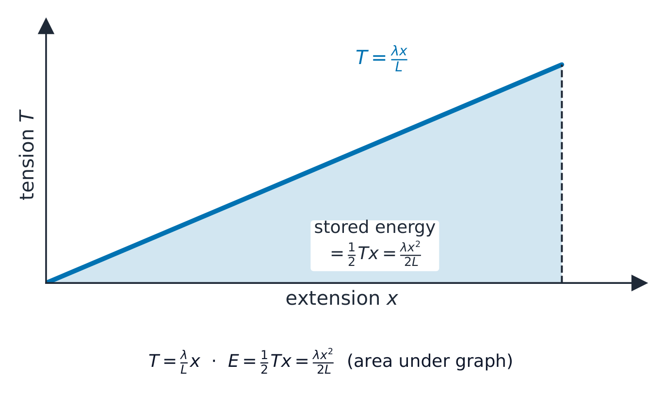
Hooke's law 胡克定律 says the tension in an elastic string or spring is proportional to its extension $x$:
$$T = \frac{\lambda x}{L},$$
where $L$ is the natural length and $\lambda$ is the modulus of elasticity 弹性模量. Stretching stores elastic potential energy 弹性势能:
$$E = \frac{\lambda x^2}{2L}.$$
Worked example. An elastic string of natural length $2\ \text{m}$ and modulus $50\ \text{N}$ is stretched by $0.5\ \text{m}$. Find the tension and the stored energy.
Force is proportional to extension — the gradient is the stiffness k. · כוח פרופורציונלי לארכיפה — השיפוע הוא הקשיחות k.
3.5
Linear motion under a variable force · תנועה קווית תחת כוח משתנה
Syllabus · סיילבוס
English
Candidates should be able to:
Notes and examples
solve problems which can be modelled as the linear motion of a particle under the action of a variable force, by setting up and solving an appropriate differential equation.
Including use of $v \frac{\mathrm{d}v}{\mathrm{d}x}$ for acceleration, where appropriate. Calculus required is restricted to content from Pure Mathematics 3 in Cambridge International A Level Mathematics (9709). Only differential equations in which the variables are separable are included.
עברית
המועמדים אמורים להיות מסוגלים:
הערות לדוגמאות
לפתור בעיות שיכולות להיות מודללות כתנועה ליניארית של חלקיק תחת השפעת כוח משתנה, על ידי הצבת ופתרון משוואה דיפרנציאלית מתאימה.
כולל שימוש ב$v \frac{\mathrm{d}v}{\mathrm{d}x}$ לתאוצה, כאשר יש צורך בכך. החשבונות הנדרשים מוגבלים לחומר מן המתמטיקה הטהורה 3 במסגרת Cambridge International A Level Mathematics (9709). כלולות רק משוואות דיפרנציאליות שהמשתנים בהן ניתנים להפרדה.
Source: Cambridge International syllabus · מקור: הסיילבוס הבינלאומי של קמבריד'ג'
English
When the force depends on position $x$, use acceleration in the form $a = v\dfrac{dv}{dx}$, which turns Newton's law into a differential equation 微分方程 relating $v$ and $x$.
Worked example. A particle of mass $8\ \text{kg}$ moves along a line under a variable force 变力 of size $(x^3 + 4x)\ \text{N}$ acting in the direction of motion. When $x = 0$, $v = 1$. Find $v$ in terms of $x$.
Newton's law gives $8v\dfrac{dv}{dx} = x^3 + 4x$. Separating and integrating:
כאשר הכוח תלוי במיקום $x$, השתמשו בהאצה בצורה $a = v\dfrac{dv}{dx}$, מה שהופך את חוק ניוטון למשוואה דיפרנציאלית המקשרת בין $v$ ל$x$.
השתמשו ב-dv/dt כאשר הכוח תלוי בזמן, וב-v·dv/dx כאשר הוא תלוי במיקום
דוגמא פתורה. חלקיק המסה $8\ \text{kg}$ נע לאורך קו תחת כוח משתנה בגודל $(x^3 + 4x)\ \text{N}$ הפועל בכיוון התנועה. כאשר $x = 0$, $v = 1$. מצאו את $v$ באמצעות $x$.
חוק ניוטן נותן $8v\dfrac{dv}{dx} = x^3 + 4x$. בידוד משתנים ואינטגרציה:
coefficient of restitution/ˌkəʊɪˈfɪʃənt ɒv rɪstɪˈtjuːʃn/
מקדם החזרה
bounding parabola/ˈbaʊndɪŋ pəˈræbələ/
פרבולה חוסמת
lamina/ˈlæmɪnə/
למינה (מלבד דו-ממדי)
coplanar forces/ˌkəʊˈpleɪnə ˈfɔːsɪz/
כוחות מצטבים
conical pendulum/ˈkɒnɪkl ˈpendjʊləm/
פנדול קוני
normal contact force/ˈnɔːml ˈkɒntækt fɔːs/
כוח מגע אנכי
oblique impact/əˈbliːk ˈɪmpækt/
התנגשות אלכסונית
3.6
Momentum · תנע
Syllabus · סיילבוס
English
Candidates should be able to:
Notes and examples
recall Newton’s experimental law and the definition of the coefficient of restitution, the property $0 \leqslant e \leqslant 1$, and the meaning of the terms ‘perfectly elastic’ ($e = 1$) and ‘inelastic’ ($e = 0$)
use conservation of linear momentum and/or Newton’s experimental law to solve problems that may be modelled as the direct or oblique impact of two smooth spheres, or the direct or oblique impact of a smooth sphere with a fixed surface.
עברית
המועמדים אמורים להיות מסוגלים:
הערות לדוגמאות
לזכור את חוק ניוסטון הניסויי והגדרת מקדם ההתאוששות, התכונה $0 \leqslant e \leqslant 1$, והמשמעות של המונחים 'אלסטי מושלם' ($e = 1$) ו'לא-אלסטי' ($e = 0$)
להשתמש בשימור תנע ליניארי וב/או בחוק ניוסטון הניסויי כדי לפתור בעיות שיכולות להיות מודללות כהתנגשות ישירה או אלכסונית של שני כדורים חלקים, או התנגשות ישירה או אלכסונית של כדור חלק עם משטח קבוע.
Source: Cambridge International syllabus · מקור: הסיילבוס הבינלאומי של קמבריד'ג'
English
In a collision, total linear momentum is conserved — the conservation of linear momentum 动量守恒. The bounciness is measured by Newton's experimental law 牛顿实验定律, which defines the coefficient of restitution 恢复系数$e$:
$$e = \frac{\text{speed of separation}}{\text{speed of approach}}, \qquad 0 \leqslant e \leqslant 1.$$
Here $e = 1$ is perfectly elastic (no energy lost) and $e = 0$ is inelastic (the bodies stay together). In an oblique impact 斜碰撞, resolve the velocities along and perpendicular to the line of impact, applying restitution along it.
Worked example. A sphere $A$ of mass $2\ \text{kg}$ moving at $5\ \text{m s}^{-1}$ hits a stationary sphere $B$ of mass $3\ \text{kg}$, with $e = 0.5$. Find the speeds afterwards.
בתהליך התנגשות, תנע ליני כולו שמר — שימור התנע הליני. גמישות התהליך נמדדת לפי חוק ניסויי של ניוטון, המגדיר את מקדם ההתאוששות$e$:
$$e = \frac{\text{speed of separation}}{\text{speed of approach}}, \qquad 0 \leqslant e \leqslant 1.$$
כאן $e = 1$ היא אלסטית לחלוטין (אין אובדן אנרגיה) ו-$e = 0$ היא אי-אלסטית (גוף נשאר מחובר). בהתנגשות אלכסונית, פירקים את המהירויות לאורך ו perpendicular לקו ההתנגשות, ומיישמים את מקדם החזרה לאורך זה.
מקדם החזרה $e$ משווה את מהירות ההפרדה בין הגופים למהירות הקרבתם.
דוגמא פתורה. כדור $A$ בעל מסה $2\ \text{kg}$ הנע במהירות $5\ \text{m s}^{-1}$ פוגע בכדור עומד $B$ בעל מסה $3\ \text{kg}$, כאשר $e = 0.5$. מצאו את המהירויות לאחר מכן.
תנע: $2(5) = 2v_A + 3v_B$, ולכן $2v_A + 3v_B = 10$. חזרה: $v_B - v_A = 0.5(5) = 2.5$. פתרון יחד נותן $v_A = 0.5\ \text{m s}^{-1}$ ו-$v_B = 3.0\ \text{m s}^{-1}$.
Explore · חקור
A collision · פגישה
Set each mass and speed, then collide them. Total momentum is conserved — see how the velocities come out. · קבעו כל מסה ומהירות, ואז התנגשו ביניהן. תנע כולל נשמר — ראו כיצד מהירויות הפליטה מתקבלות.
3.6
Exam tips · טיפים לבחינות
English
For projectiles, resolve into horizontal (constant velocity) and vertical ($a = g$) motion, linked by the same time.
For a rigid body in equilibrium, take moments about a point that removes an unknown force.
For circular motion, use $F = mv^2/r = m\omega^2 r$ towards the centre; in a vertical circle check the minimum speed at the top.
With a variable force, use $a = v\,\frac{dv}{dx}$ and integrate; elastic PE $= \frac{\lambda x^2}{2L}$.
עברית
עבור גופי זריקה, פירוק לתנועה אופקית (מהירות קבועה) ואנכית ($a = g$), הקשורות על ידי אותו זמן.
עבור גוף מוצק בשיווי משקל, לוקחים מומנטים סביב נקודה שמבטלת כוח לא ידוע.
עבור תנועה מעגלית, משתמשים ב-$F = mv^2/r = m\omega^2 r$ לכיוון המרכז; במעגל אנכי בודקים את המהירות המינימלית בראש.
עם כוח משתנה, משתמשים ב-$a = v\,\frac{dv}{dx}$ ואינטגרלים; אנרגיה פוטנציאלית אלסטית $= \frac{\lambda x^2}{2L}$.
4
Further Probability & Statistics · סיכום והסתברות נוספים
This handout covers Topic 4: Further Probability & Statistics 进阶概率统计. It adds continuous distributions, small-sample inference, the chi-squared and non-parametric tests, and probability generating functions.
4.1
Continuous random variables
Syllabus · סיילבוס
English
Candidates should be able to:
Notes and examples
use a probability density function which may be defined piecewise
use the general result $\text{E}(g(X)) = \int f(x)g(x) \, \mathrm{d}x$ where $f(x)$ is the probability density function of the continuous random variable $X$ and $g(X)$ is a function of $X$
understand and use the relationship between the probability density function (PDF) and the cumulative distribution function (CDF), and use either to evaluate probabilities or percentiles
use cumulative distribution functions (CDFs) of related variables in simple cases.
e.g. given the CDF of a variable $X$, find the CDF of a related variable $Y$, and hence its PDF, e.g. where $Y = X^3$.
עברית
המועמדים אמורים להיות מסוגלים:
הערות לדוגמאות
להשתמש בפונקציית צפיפות הסתברות שעשויה להיות מוגדרת במקטעים
להשתמש בתוצאה הכללית $\text{E}(g(X)) = \int f(x)g(x) \, \mathrm{d}x$ כאשר $f(x)$ היא פונקציית צפיפות ההסתברות של המשתנה הרנדומלי הרציף $X$ ו$g(X)$ היא פונקציה של $X$
להבין ולהשתמש בקשר בין פונקציית צפיפות ההסתברות (PDF) לבין פונקציית ההתפלגות המצטברת (CDF), ולהשתמש באחת מהן כדי לחשב הסתברויות או אחוזונים
להשתמש בפונקציות התפלגות מצטברת (CDFs) של משתנים קשורים במקרים פשוטים.
לדוגמה: נתונה CDF של משתנה $X$, מצאו את ה-CDF של משתנה קשור $Y$, ומכאן את ה-PDF שלו, לדוגמה כאשר $Y = X^3$.
Source: Cambridge International syllabus · מקור: הסיילבוס הבינלאומי של קמבריד'ג'
A continuous variable $X$ is described by a probability density function 概率密度函数$f(x)$, which may be defined piecewise. The probability over a range is the area under $f$, and the mean of any function of $X$ is
$$E(g(X)) = \int g(x)\,f(x)\,dx.$$
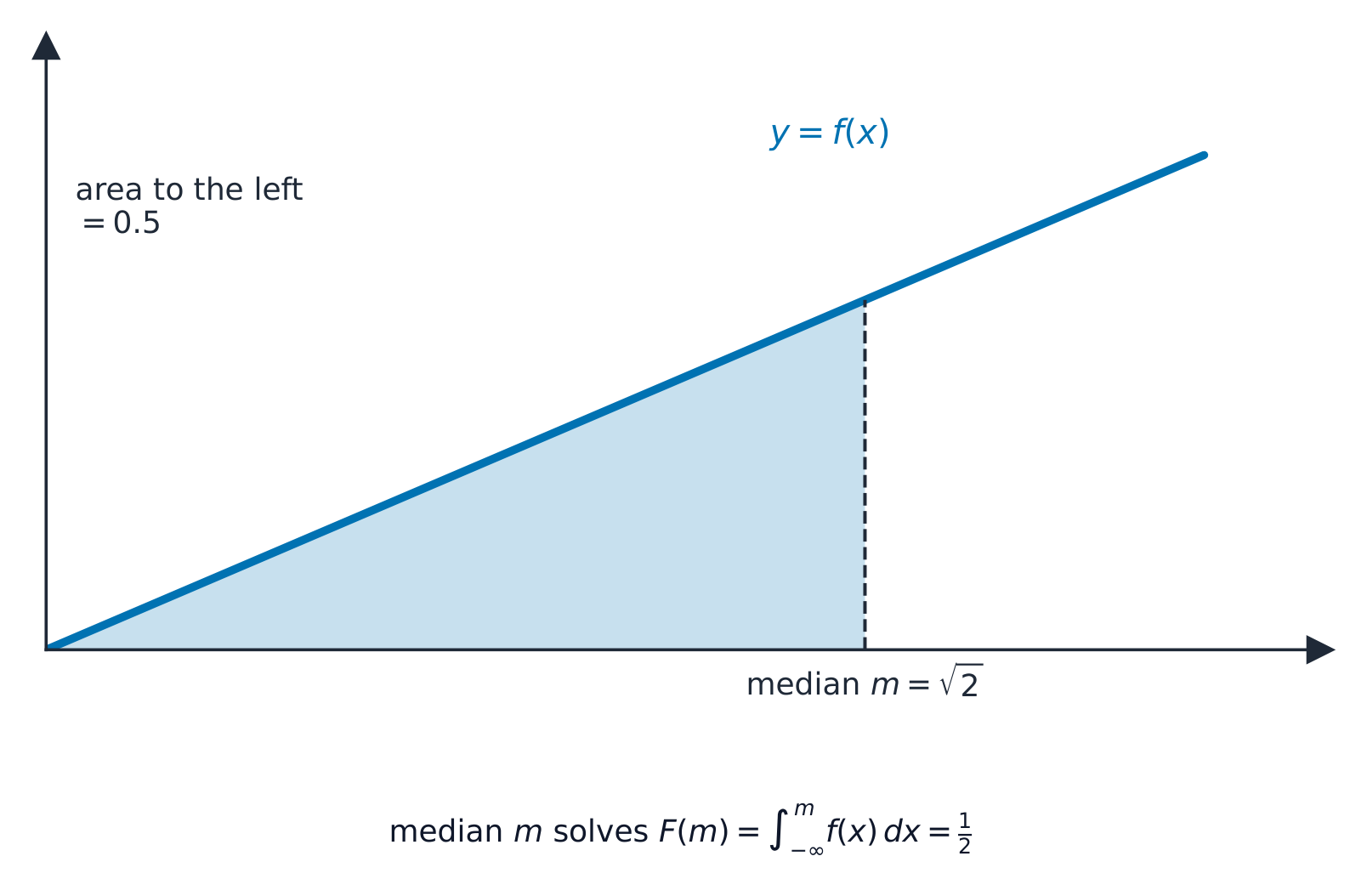
The median sits where the area under $f(x)$ to its left is exactly $0.5$.
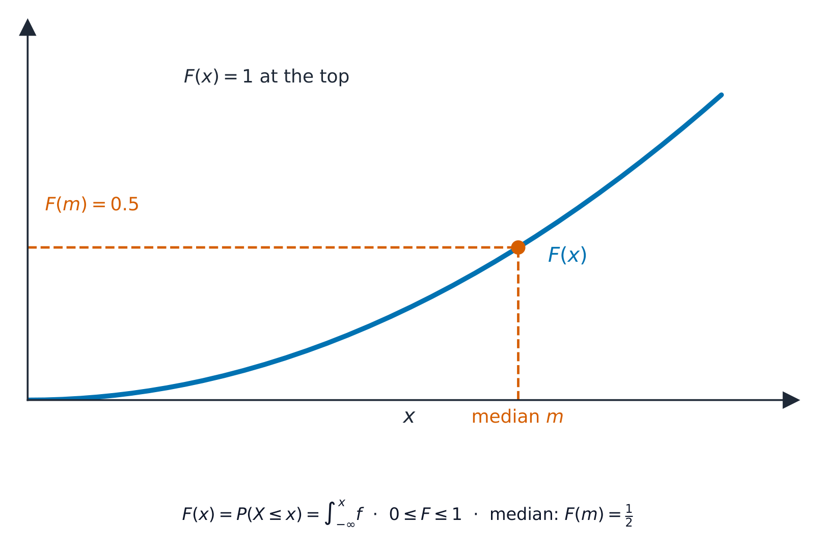
The cumulative distribution function 累积分布函数$F(x) = P(X \leqslant x)$ is the running total: $F(x) = \displaystyle\int_{-\infty}^{x} f(t)\,dt$, and $f(x) = F'(x)$. Use $F$ to find probabilities and percentiles 百分位数 (for example, the median 中位数 solves $F(x) = 0.5$).
The cumulative graph $F(x)$ rises from $0$ to $1$; the height $0.5$ is reached at the median.
Worked example. A variable has $f(x) = \tfrac12 x$ for $0 \leqslant x \leqslant 2$. Find the median.
The cumulative distribution function is $F(x) = \displaystyle\int_0^x \tfrac12 t\,dt = \tfrac14 x^2$. Set $F(m) = 0.5$:
The distribution of a related variable. If $Y=g(X)$, find $Y$'s distribution through its cumulative function. For $Y=X^2$: $F_Y(y)=P(X^2\leqslant y)=P(-\sqrt y\leqslant X\leqslant\sqrt y)=F_X(\sqrt y)-F_X(-\sqrt y)$, then differentiate for $f_Y=F_Y'$. When $g$ is monotonic increasing there is a shortcut, $F_Y(y)=F_X\big(g^{-1}(y)\big)$.
Worked example. With $f_X(x)=\tfrac12 x$ on $[0,2]$ (so $F_X(x)=\tfrac14 x^2$), let $Y=X^2$. For $0\leqslant y\leqslant 4$, $F_Y(y)=F_X(\sqrt y)=\tfrac14 y$, so $f_Y(y)=F_Y'(y)=\tfrac14$ – that is, $Y$ is uniform on $[0,4]$.
Explore · חקור
Continuous random variables · משתנים מקריים רציפים
P(a < X < b) = ∫ f(x) dx
For a continuous variable, probability is the area under the density curve. · למשתנה רציף, הסתברות היא ה-שטח מתחת לעקומת הצפיפות.
probability density function/ˌprɒbəˈbɪlɪti ˈdensɪti ˈfʌŋkʃn/
פונקציית צפיפות הסתברות
cumulative distribution function/ˈkjuːmjʊlətɪv ˌdɪstrɪˈbjuːʃn ˈfʌŋkʃn/
פונקציית ההתפלגות המצטברת
percentiles/pəˈsentaɪlz/
אחוזונים
median/ˈmiːdiːən/
חציון
4.2
Inference using normal and t-distributions
Syllabus · סיילבוס
Candidates should be able to:
Notes and examples
formulate hypotheses and apply a hypothesis test concerning the population mean using a small sample drawn from a normal population of unknown variance, using a t-test
calculate a pooled estimate of a population variance from two samples
Calculations based on either raw or summarised data may be required.
formulate hypotheses concerning the difference of population means, and apply, as appropriate: - a 2-sample t-test - a paired sample t-test - a test using a normal distribution
The ability to select the test appropriate to the circumstances of a problem is expected.
determine a confidence interval for a population mean, based on a small sample from a normal population with unknown variance, using a t-distribution
determine a confidence interval for a difference of population means, using a t-distribution or a normal distribution, as appropriate.
Source: Cambridge International syllabus · מקור: הסיילבוס הבינלאומי של קמבריד'ג'
A Galton board: balls falling through pins pile up into the bell-shaped normal distribution.
When a sample is small and the population variance is unknown, base your hypothesis test 假设检验 on the $t$-distribution instead of the normal. The same idea gives a confidence interval 置信区间 for the mean:
$$\bar{x} \pm t\,\frac{s}{\sqrt{n}},$$
where $t$ comes from the $t$-tables with $n - 1$ degrees of freedom. To compare two populations, use a two-sample (2-sample) or paired-sample$t$-test, after finding a pooled estimate 合并估计 of the shared variance when appropriate.
For a small sample the $t$-distribution is flatter with heavier tails, so its critical values are larger.
Worked example. A sample of $n = 10$ has mean $\bar{x} = 50$ and standard deviation $s = 4$. Find a $95\%$ confidence interval for the mean (use $t = 2.262$ for $9$ degrees of freedom).
Why small samples need t instead of z · מדום דגימות קטנות יש להשתמש ב-t במקום ב-z
With $\sigma$ unknown you use $t$, and $t$ has heavier tails than the normal (drawn dashed behind it) — so its critical values are larger and the interval is wider. At the worked example's $9$ degrees of freedom the widget reads $t^* = 2.262$, exactly the table value used above. Sweep df up and $t$ collapses onto the normal. · כאשר יש לך $\sigma$ לא ידועים, משתמשים ב-$t$, ול-$t$ יש זנבות כבדים יותר מאשר הנורמלי (מצויר בקו מקווקוה מאחוריו) — ולכן הערכים הקריטיים שלו הם גדולים יותר והמרווח רחב יותר. במעבר לדוגמה המפורטת עם $9$ דרגות חופש, הווידג'ט מציג $t^* = 2.262$, בדיוק כמו הערך בטבלה שהשתמשנו בו למעלה. גרור את df כלפי מעלה וה-$t$ מתכנס אל הנורמלי.
Explore · חקור
The normal distribution · החלוקה הנורמלית
Shade a tail to find a probability — the basis of confidence intervals and hypothesis tests. · צללו זנב כדי למצוא הסתברות — זהו הבסיס למרווחי אמון ולמבחני הישגיות.
fit a theoretical distribution, as prescribed by a given hypothesis, to given data
Questions will not involve lengthy calculations.
use a $\chi^2$-test, with the appropriate number of degrees of freedom, to carry out the corresponding goodness of fit analysis
Classes should be combined so that each expected frequency is at least 5.
use a $\chi^2$-test, with the appropriate number of degrees of freedom, for independence in a contingency table.
Yates’ correction is not required. Where appropriate, either rows or columns should be combined so that the expected frequency in each cell is at least 5.
עברית
המועמדים אמורים להיות מסוגלים:
הערות לדוגמאות
התאמת חלוקה תיאורטית, כפי שנקבע על ידי הנחת יסוד נתונה, לנתונים הנתונים
השאלות לא יכללו חישובים ארוכים.
ביצוע מבחן $\chi^2$, עם מספר הדרגות החופשי המתאים, לבצע את אנליזת ההתאמה הטובה ההתאמת
יש לשלב מחלקות כך שתדירות מצופה בכל אחת תהיה לפחות 5.
ביצוע מבחן $\chi^2$, עם מספר הדרגות החופשי המתאים, לבדיקת עצמאות בטבלת קונטינגנצי.
אינו נדרש תיקון יייטס. כאשר מתאים, יש לשלב שורות או עמודות כך שתדירות מצופה בתא כלשהו תהיה לפחות 5.
Source: Cambridge International syllabus · מקור: הסיילבוס הבינלאומי של קמבריד'ג'
A $\chi^2$-test (chi-squared test 卡方检验) compares observed counts $O$ with expected counts $E$ from a theoretical distribution 理论分布:
$$\chi^2 = \sum \frac{(O - E)^2}{E}.$$
Compare this with a table value for the right number of degrees of freedom 自由度. Two uses: a goodness of fit 拟合优度 test (does the data follow the proposed model?), and a test for independence 独立性 of two variables in a contingency table 列联表.
The test rejects the model when $\chi^2$ exceeds the critical value, landing in the shaded $5\%$ tail.
Worked example. Four equally likely categories give observed counts $20, 30, 25, 25$ (so each expected count is $25$). Test the fit at the $5\%$ level.
With $4 - 1 = 3$ degrees of freedom the table value is $7.815$. Since $2 < 7.815$, do not reject the model.
Explore · חקור
The chi-squared distribution and its 5% tail · התפלגות קי-ריבוע והזנב ה-5% שלה
The worked example on this page gives $\chi^2 = 2$ with $3$ degrees of freedom against a table value of $7.815$ — the widget reproduces both. Drag df to see why the critical value changes with the number of categories. · הדוגמה המפורטת בדף מציגה $\chi^2 = 2$ עם $3$ דרגות חופש לעומת ערך טבלאי של $7.815$ — הווידג'ט משחזר את שניהם. גרור את df כדי לראות מדוע הערך הקריטי משתנה בהתאם למספר הקטגוריות.
Explore · חקור
Chi-squared test route · דרך מבחן קי-ריבוע
Follow observed and expected counts to a test decision. · עקוב אחר ספירות מצופות ומצופות להחלטת מבחן.
understand the idea of a non-parametric test and appreciate situations in which such a test might be useful
e.g. when sampling from a population which cannot be assumed to be normally distributed.
understand the basis of the sign test, the Wilcoxon signed-rank test and the Wilcoxon rank-sum test
Including knowledge that Wilcoxon tests are valid only for symmetrical distributions.
use a single-sample sign test and a single-sample Wilcoxon signed-rank test to test a hypothesis concerning a population median
Including the use of normal approximations where appropriate. Questions will not involve tied ranks or observations equal to the population median value being tested.
use a paired-sample sign test, a Wilcoxon matched-pairs signed-rank test and a Wilcoxon rank-sum test, as appropriate, to test for identity of populations.
Including the use of normal approximations where appropriate. Questions will not involve tied ranks or zero‑difference pairs.
עברית
המועמדים אמורים להיות מסוגלים:
הערות לדוגמאות
הבנת הרעיון של מבחן פארמטרי והיכרות עם מצבים שבהם מבחן כזה עשוי להיות שימושי
לדוגמה: בעת דגימה מאוכלוסייה שאין להניח שהיא חלוקה נורמלית.
הבנת היסוד של מבחן הסימן, מבחן דירוג הסימן של וילקוקסון ומבחן סך הדירוגים של וילקוקסון
כולל ידע בכך שמבחני וילקוקסון תקפים רק לחלוקות סימטריות.
שימוש במבחן סימן למדגם יחיד ובמבחן דירוג הסימן של וילקוקסון למדגם יחיד, כדי לבדוק הנחה לגבי מדiane האוכלוסייה
כולל שימוש בקירובים נורמליים כאשר מתאים. השאלות לא יכללו דירוגים זרים או תצפיות השוות לערך המדiane של האוכלוסייה הנבדק.
שימוש במבחן סימן למדגם זוגי, במבחן דירוג הסימן של וילקוקסון למדגם זוגי ובמבחן סך הדירוגים של וילקוקסון, בהתאם, כדי לבדוק זהות אוכלוסיות.
כולל שימוש בקירובים נורמליים כאשר מתאים. השאלות לא יכללו דירוגים זרים או זוגות עם הפרש אפס.
Source: Cambridge International syllabus · מקור: הסיילבוס הבינלאומי של קמבריד'ג'
A non-parametric test 非参数检验 makes no assumption that the data is normal, so it is useful when that assumption fails. The basic ones are:
the sign test 符号检验: count how many values fall above and below a proposed median, and test those counts with a binomial model;
the Wilcoxon signed-rank test 威尔科克森符号秩检验 (the matched-pairs test for paired data), which also uses the sizes of the differences, not just their signs;
the Wilcoxon rank-sum test 威尔科克森秩和检验, for comparing two separate samples.
The sign test counts how many values fall above and below the proposed median, then tests those counts with a binomial model
Worked example. Test whether a median is $5$. In a sample of $10$ values (none equal to $5$), $9$ lie above$5$ and $1$ lies below. Test at the $5\%$ level (two-tailed).
Under $H_0$ (median $= 5$) the number above follows $B(10, 0.5)$. The observed result ($9$ above) is extreme, so find $P(X \geq 9) = \binom{10}{9}(0.5)^{10} + (0.5)^{10} = \dfrac{11}{1024} = 0.0107$. For a two-tailed test compare with $\tfrac{1}{2}(5\%) = 0.025$. Since $0.0107 < 0.025$, reject $H_0$: there is evidence the median is not $5$.
Explore · חקור
Non-parametric test chooser · בוחר מבחן לא פרמטרי
Choose the rank-based test that matches the data situation. · בחרו את המבחן המבוסס על רתימות המתאים למצב הנתונים.
understand the concept of a probability generating function (PGF) and construct and use the PGF for given distributions
Including the discrete uniform, binomial, geometric and Poisson distributions.
use formulae for the mean and variance of a discrete random variable in terms of its PGF, and use these formulae to calculate the mean and variance of a given probability distribution
use the result that the PGF of the sum of independent random variables is the product of the PGFs of those random variables.
עברית
המועמדים אמורים להיות מסוגלים:
הערות לדוגמאות
הבנת מושג פונקציית יצירת הסתברות (PGF) והרכבה ושימוש בפונקציה זו לחלוקות נתונות
כולל החלוקה האחידה הדיסקרטית, הבינומית, הגיאומטרית והפואסון.
שימוש בנוסחאות עבור הממוצע והשונות של משתנה מקרי דיסקרטי במונחי ה-PGF שלה, ושימוש בנוסחאות אלו לחישוב הממוצע והשונות של חלוקת הסתברות נתונה
שימוש בתוצאה לפיה ה-PGF של סכום משתנים מקריים בלתי תלויים הוא מכפלת ה-PGFs של משתנים אלו.
Source: Cambridge International syllabus · מקור: הסיילבוס הבינלאומי של קמבריד'ג'
Dice: a starting point for probability and discrete random variables.
The probability generating function 概率母函数 of a discrete variable $X$ is
$$G(t) = E(t^X) = \sum_x P(X = x)\,t^x.$$
It packs the whole distribution into one function. The mean and variance come from its derivatives at $t = 1$: $E(X) = G'(1)$ and $\mathrm{Var}(X) = G''(1) + G'(1) - \big(G'(1)\big)^2$. Also, the PGF of a sum of independent variables is the product of their PGFs.
Worked example.$X$ has $P(X=0) = 0.5$, $P(X=1) = 0.3$, $P(X=2) = 0.2$. Find $E(X)$ using the PGF.
Here $G(t) = 0.5 + 0.3t + 0.2t^2$, so $G'(t) = 0.3 + 0.4t$ and
$$E(X) = G'(1) = 0.3 + 0.4 = 0.7.$$
PGF of a fair die packs equal masses at 1 through 6 into G(t)
Explore · חקור
Probability generating function lab · מעבדת פונקציית יצירת הסתברות
G(x) = p0 + p1 x + p2 x^2 + ...
Change x and see how a PGF stores probabilities in powers of x. · שנה ב-x וראה כיצד PGF מאחסן סיכומי הסתברות כחזקות של x.
Pick one and the site follows you — notes, papers, videos and practice all open on it. · בחרו נושא אחד והאתר יעקוב אחריו — הערות, מסמכים, וידאו ותרגולים פתוחים בו.
Type to search notes, lessons, code, vocabulary and past-paper questions across every subject. · הקלד כדי לחפש הערות, שיעורים, קוד, אוצר מילים ושאלות מבחנים בכל הנושאים.