ספר טלפונים עם מיליון שמות. אם תבדוק אותם אחד אחד, ייתכן שתבצע מיליון השוואות. אבל כבר ידוע לך הטריק: פתח אותו בחצי…
English narration · English + 中文 subtitles burned in · קריאת קול באנגלית · תרגום אנגלי + סינית שרוף בתוך הסרטון
19.1
Searching algorithms · אלגוריתמי חיפוש
Syllabus · סיילבוס
English
Candidates should be able to:
Notes and guidance
Show understanding of linear search and binary search methods
Write an algorithm to implement a linear search Write an algorithm to implement a binary search The conditions necessary for the use of a binary search How the performance of a binary search varies according to the number of data items
Show understanding of insertion sort and bubble sort methods
Write an algorithm to implement an insertion sort Write an algorithm to implement a bubble sort Performance of a sorting routine may depend on the initial order of the data and the number of data items
Show understanding of and use Abstract Data Types (ADT)
Write algorithms to find an item in each of the following: linked list, binary tree Write algorithms to insert an item into each of the following: stack, queue, linked list, binary tree Write algorithms to delete an item from each of the following: stack, queue, linked list Show understanding that a graph is an example of an ADT. Describe the key features of a graph and justify its use for a given situation. Candidates will not be required to write code for a graph structure
Show how it is possible for ADTs to be implemented from another ADT
Describe the following ADTs and demonstrate how they can be implemented from appropriate built-in types or other ADTs: stack, queue, linked list, dictionary, binary tree
Show understanding that different algorithms which perform the same task can be compared by using criteria (e.g. time taken to complete the task and memory used)
Including use of Big O notation to specify time and space complexity
עברית
המועמדים צריכים להיות מסוגלים:
הערות והנחיות
להראות הבנה של linear search ו-binary search
כתוב אלגוריתם ליישום linear search. כתוב אלגוריתם ליישום binary search. התנאים הנדרשים לשימוש ב-binary search. איך הביצועים של binary search משתנים בהתאם למספר פריטי הנתונים
להראות הבנה של insertion sort ו-bubble sort
כתוב אלגוריתם ליישום insertion sort. כתוב אלגוריתם ליישום bubble sort. ביצועי פעולת מיון עשויים להסתמך על הסדר ההתחלתי של הנתונים ומספר פריטי הנתונים
להראות הבנה ושימוש ב-Abstract Data Types (ADT)
כתוב אלגוריתמים למציאת פריט בכל אחד מ: linked list, binary tree. כתוב אלגוריתמים להכנסת פריט לכל אחד מ: stack, queue, linked list, binary tree. כתוב אלגוריתמים למחיקת פריט מכל אחד מ: stack, queue, linked list. הראה הבנה ש-גרף הוא דוגמה ל-ADT. תאר את התכונות המרכזיות של גרף והסבר את שימושו למצב נתון. תלמידים לא ידרשו לכתוב קוד למבנה גרף
להראות כיצד ADTs ניתן ליישם באמצעות ADT אחר
תאר את ADTs הבא והראה כיצד ניתן ליישם אותם מסוגים מובנים או ADTs אחרים מתאימים: stack, queue, linked list, dictionary, binary tree
להראות הבנה שאפשר להשוות בין אלגוריתמים שונים המבצעים אותו משימה באמצעות קריטריונים (למשל זמן ביצוע השיטה והזיכרון המשמש)
כולל שימוש ב-Big O notation כדי לציין מורכבות זמן ומרחב
Source: Cambridge International syllabus · מקור: הסיילבוס הבינלאומי של קמבריד'ג'
English
Big O: how algorithms scaleInsertion sort: slide each card into placeBubble sort, pass by passBinary search: halve and conquer
A search finds a target value in a collection (often an array 数组) and returns its position, or "not found".
Linear search
A linear search 线性查找 walks from start to end, comparing each element with the target:
No preparation is needed, so it works on any list. Worst case O($n$) (target at the end or absent); best case 1 comparison. Use it on unsorted data or small lists. (The returned -1 is a sentinel value — an impossible position that means "not found"; the caller tests IF result = -1.)
The exam's version. Paper 3 asks you to complete a linear search written with a flag and a WHILE loop, and Paper 4 to write a function that returns the index or a count. Both look like this:
To stop at the first match instead, use a WHILE Index <= 100 AND NOT Found loop that sets Found ← TRUE and remembers the index. The marks are for the loop over every element, the comparison, and what is returned when the value is absent.
Binary search
A binary search 二分查找 needs the data sorted. Look at the middle element; if it is the target, done; if the target is smaller, search the left half, else the right half — halving the range each time:
Worst case O($\log_{2} n$) — for a million items, about 20 comparisons. Much faster than linear search on large sorted arrays, but you must sort first (a one-off O($n \log n$) cost), worth it if you search many times.
"State the condition necessary for a binary search."The data must be in order (sorted, ascending or descending, on the key being searched). "Describe how to perform a binary search" (three marks): (1) find the middle item of the list (or of the current range) and compare it with the target; (2) if it matches, the search ends; if the target is smaller, repeat on the lower half, if larger, on the upper half; (3) keep halving the range until the item is found or the range is empty, which means it is not present.
The exam's version, with the bounds and a flag, is the one to reproduce when asked to complete the algorithm:
"Explain how the performance varies with the number of items." Each comparison halves the number of items left, so the maximum number of comparisons is about $\log_{2} n$: doubling the size of the list adds only one more comparison. This is O($\log n$). "Compare linear and binary search": a linear search needs up to $n$ comparisons (O($n$)) and, on average, half that, but works on unsorted data; a binary search needs at most $\log_{2} n$ (O($\log n$)) and is far faster for large lists, but the data must first be sorted and it must allow direct access to the middle item (an array, not a linked list). For $1000$ items: $1000$ against $10$ comparisons.
עברית
Big O: כיצד אלגוריתמים מתרחביםסינון הכנסה: החלקת כל כרטיס למקומומיון בועות, מעבר אחר מעברחיפוש בינארי: חלוקה לשתיים וכיבוש
חיפוש מוצא ערך יעד בקבוצת נתונים (לרוב מערך) ומחזיר את מיקומו, או "לא נמצא".
חיפוש ברשימה מסודרת, כמו מדריך טלפונים, מהיר משמעותית מבדיקה של כל פנייה בנפרד
חיפוש ליניארי
חיפוש ליניארי עובר מאחד הקצה ל另一端, ומשווה כל אלמנט ליעד:
FOR i ← 1 TO n
    IF A[i] = target THEN
        RETURN i
    ENDIF
NEXT i
RETURN -1   // not found
אין צורך בהכנה, ולכן זה עובד על כל רשימה. מקרה גרוע O($n$) (היעד בסוף או שאינו קיים); מקרה טוב 1 השוואה. השתמש בו בנתונים לא מסודרים או ברשימות קטנות. (ה--1 המוחזר הוא ערך שלט — מיקום בלתי אפשרי שמעניין "לא נמצא"; הקורא בודק IF result = -1.)
הגרסה במבחן. בבחן 3 עליך להשלים חיפוש ליניארי שנכתב עם דגל וWHILE לולאה, ובבחן 4 לכתוב פונקציה שהמחזירה אינדקס או ספירה. שניהם נראים כך:
FUNCTION LinearSearch(Data : ARRAY OF INTEGER, Target : INTEGER) RETURNS INTEGER
    DECLARE Index, Count : INTEGER
    Count ← 0
    FOR Index ← 1 TO 100
        IF Data[Index] = Target THEN
            Count ← Count + 1
        ENDIF
    NEXT Index
    RETURN Count          // how many times Target occurs; 0 means not found
ENDFUNCTION
כדי לעצור בתוצאה הראשונה במקום זאת, השתמש בWHILE Index <= 100 AND NOT Found לולאה שמגדירה Found ← TRUE ושומרת על האינדקס. הנקודות הן עבור הלולאה על כל אלמנט, ההשוואה, והמה שמוחזר כאשר הערך לא קיים.
חיפוש ליניארי בודק כל אות בתור — 23 השוואות כדי למצוא W
חיפוש בינארי
חיפוש בינארי דורש שהנתונים יהיו מסודרים. התבונן באלמנט האמצעי; אם הוא היעד, הגמר; אם היעד קטן יותר, חפש בחצי השמאלי, אחרת בחצי הימני — מחלק את הטווח בכל פעם:
low ← 1
high ← n
WHILE low <= high DO
    mid ← (low + high) DIV 2
    IF A[mid] = target THEN
        RETURN mid
    ENDIF
    IF A[mid] < target THEN
        low ← mid + 1
    ELSE
        high ← mid - 1
    ENDIF
ENDWHILE
RETURN -1
מקרה גרוע O($\log_{2} n$) — עבור מיליון פריטים, כ-20 השוואות. מהיר משמעותית מחיפוש ליניארי על מערכים מסודרים גדולים, אך יש לסדר קודם לכן (עלות חד-פעמית של O($n \log n$)), מה ששווה את העדפה אם מבצעים חיפוש רבות.
"ציינו את התנאי הנדרש לחיפוש בינארי." הנתונים חייבים להיות במערכת סידור (מסודרים, בעלייה או ירידה, לפי המפתח שנחפש). "תארו כיצד לבצע חיפוש בינארי" (שלוש נקודות): (1) מצאו את הפריט האמצעי ברשימה (או בטווח הנוכחי) והשוו אותו למטרה; (2) אם הוא תואם, החיפוש מסתיים; אם המטרה קטנה יותר, חזרו על פעולה בחצי התחתון, ואם גדולה יותר, בחצי העליון; (3) המשיכו בחצירת הטווח עד שמצאים את הפריט או שהטווח מתרוקש, דבר המעיד שאינו קיים.
הגרסה של הבחינה, עם הגבולות ודגל, היא זו שיש לשחזר כאשר מבקשים להשלם את האלגוריתם:
DECLARE Lower, Upper, Mid : INTEGER
DECLARE Found : BOOLEAN
Lower ← 0
Upper ← 99
Found ← FALSE
WHILE Lower <= Upper AND NOT Found
    Mid ← (Lower + Upper) DIV 2
    IF Names[Mid] = Target THEN
        Found ← TRUE
    ELSE
        IF Names[Mid] < Target THEN
            Lower ← Mid + 1
        ELSE
            Upper ← Mid - 1
        ENDIF
    ENDIF
ENDWHILE
IF Found THEN
    OUTPUT Mid
ELSE
    OUTPUT "Not found"
ENDIF
"הסבירו כיצד הביצועים משתנים בהתאם למספר הפריטים." כל השוואה חותכת בחצי את מספר הפריטים שנותרו, ולכן המקסימום בשומות ההשוואות הוא כ-$\log_{2} n$: הכפלת גודל הרשימה מוסיפה רק אחת השוואה נוספת. זהו O($\log n$). "השוו בין חיפוש ליניארי לחיפוש בינארי:" חיפוש ליניארי זקוק עד $n$ השוואות (O($n$)) ובמידה הממוצעת חצי מכך, אך עובד על נתונים לא מסודרים; חיפוש בינארי זקוק עד $\log_{2} n$ (O($\log n$)) ומהיר משמעותית ברשימות גדולות, אך הנתונים חייבים להיות קודם לכן מסודרים ועליהם לאפשר גישה ישירה לפריט האמצעי (מערך, ולא רשימה מקושרת). עבור $1000$ פריטים: $1000$ מול $10$ השוואות.
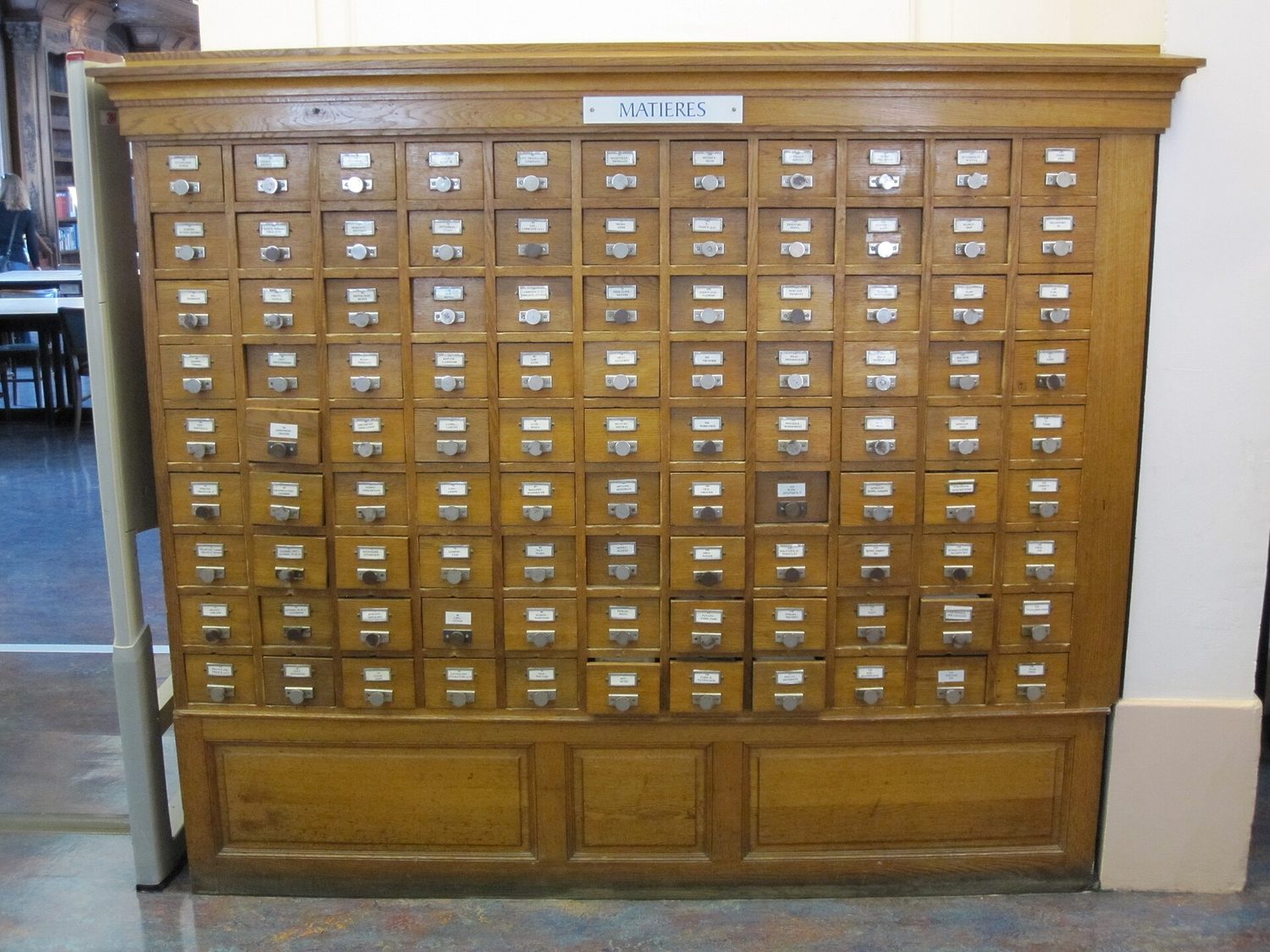
חיפוש בינארי חוצה את הטווח בכל צעד (נמוך / אמצע / גבוה) — רק 3 השוואות כדי למצוא את Wקטלוג כרטיסים: רשומות מסודרות הן מה שמאפשר חיפוש בינארי — חצו, בדקו, חצו שוב
Explore · חקור
Linear vs binary search · חיפוש ליניארי לעומת חיפוש בינארי
Search for a value. Binary search halves the list each step (only on sorted data); linear search checks one by one. · חפש ערך מסוים. חיפוש בינארי מחלק את הרשימה למחצה בכל שלב (רק על נתונים מסודרים); חיפוש ליניארי בודק אלמנט אחד אחר השני.
A bubble sort 冒泡排序 repeatedly walks the array, swapping adjacent pairs that are out of order, so the largest "bubbles" to the end each pass:
Best case O($n$) (already sorted, with the early exit); average/worst O($n^{2}$). Simple but slow for large $n$.
Insertion sort
An insertion sort 插入排序 builds a sorted prefix from the left, inserting each new element into place by shifting larger ones right:
Best case O($n$) (already sorted); worst O($n^{2}$). Good for small or nearly-sorted arrays. It sorts in place 原地 and is stable 稳定 (keeps the order of equal elements).
Tracing a sort
A common task is to show the array after each outer pass. For [D, T, H, R] with insertion sort: pass 1 (key T) no change; pass 2 (key H) → [D, H, T, R]; pass 3 (key R) → [D, H, R, T].
Writing a sort from scratch. "Write pseudocode to sort DataArray[1:1000] into ascending order" is answered by a complete bubble sort with the early-exit flag, or an insertion sort, declared and indented; either scores full marks if it works for every input:
For descending order change > to <; to sort records or a 2D array by one field, compare that field but swap the whole record (or every column). Asked to write an insertion sort "that performs the same task" as a given bubble sort, keep the same array name and direction and reproduce the insertion sort above with the comparison reversed if the order is descending.
"Describe two ways the performance of a sort is affected by the data" (two marks). (1) The number of items: an $O(n^{2})$ sort takes four times as long for twice as many items. (2) How far the data is already in order: a bubble sort with a flag, or an insertion sort, finishes in one pass over already-sorted data ($O(n)$) and does the most work on data in reverse order; the number of swaps depends on how many pairs are out of order. (Also accepted: the range or number of duplicate values, and whether the items are large records that are expensive to move.) Bubble and insertion sort are both O($n^{2}$) in the worst and average cases and O($n$) at best; quicksort and merge sort are O($n \log n$), which is why they are used for large data.
עברית
סידור בועות
סידור בועות עובר שוב ושוב על המערך, ומחליף זוגות שכנים שאינם במערכת סידור, כך שהערכים הגדולים ביותר "מתנפחים" לקצה בכל מעבר:
FOR pass ← 1 TO n - 1
    swapped ← FALSE
    FOR i ← 1 TO n - pass
        IF A[i] > A[i + 1] THEN
            temp ← A[i]
            A[i] ← A[i + 1]
            A[i + 1] ← temp
            swapped ← TRUE
        ENDIF
    NEXT i
    IF swapped = FALSE THEN      // already sorted
        EXIT FOR
    ENDIF
NEXT pass
מקרה מיטבי O($n$) (כבר מסודר, עם יציאה מוקדפת); ממוצע/גרוע O($n^{2}$). פשוט אך איטי עבור מערכים גדולים $n$.
סידור הזרקה
סידור הזרקה בונה קדמה מסודרת משמאל, ומזריק כל פריט חדש למקומו על ידי הזזה של ערכים גדולים יותר ימינה:
FOR i ← 2 TO n
    key ← A[i]
    j ← i - 1
    WHILE j >= 1 AND A[j] > key DO
        A[j + 1] ← A[j]
        j ← j - 1
    ENDWHILE
    A[j + 1] ← key
NEXT i
מקרה מיטבי O($n$) (כבר מסודר); גרוע O($n^{2}$). טוב לערכים קטנים או קריב למערכת סידור. הוא מסדר בתוך המערך והוא יציב (שומר על סדר הפריטים השווים).
מעקב אחר סידור
משימה נפוצה היא להציג את המערך לאחר כל מעבר חיצוני. עבור ⟨[D, T, H, R]⟩ עם סידור הזרקה: מעבר 1 (מפתח T) ללא שינוי; מעבר 2 (מפתח H) → ⟨[D, H, T, R]⟩; מעבר 3 (מפתח R) → ⟨[D, H, R, T]⟩.
כתיבת סידור מאפס. "כתבו פסאודוקוד לסדר ⟨DataArray[1:1000]⟩ בעלייה" עונה עליו סידור בועות מלא עם דגל ליציאה מוקדפת, או סידור הזרקה, המוגדרים וממוזזים; שניהם זוכים בנקודות מלאות אם הם עובדים לכל הקלט:
DECLARE Pass, Index, Temp : INTEGER
DECLARE Swapped : BOOLEAN
Pass ← 1
REPEAT
    Swapped ← FALSE
    FOR Index ← 1 TO 1000 - Pass
        IF DataArray[Index] > DataArray[Index + 1] THEN
            Temp ← DataArray[Index]
            DataArray[Index] ← DataArray[Index + 1]
            DataArray[Index + 1] ← Temp
            Swapped ← TRUE
        ENDIF
    NEXT Index
    Pass ← Pass + 1
UNTIL Swapped = FALSE OR Pass = 1000
עבור סדר יורד שנה > ל-<; למיין רשומות או מערך דו-ממדי 2 לפי שדה אחד, השוו את השדה אך החלף את הרשומה השלמה (או כל עמודה). בבקשה לכתוב אלגוריתם insertion sort "העושה אותו עבודה" כמו bubble sort נתון, שמור את אותו שם מערך וכיוון והעתק את insertion sort לעיל עם ההשוואה הפוכה אם הסדר הוא יורד.
"תארו שתי דרכים שבהן ביצועי הסידור מושפעים מהנתונים" (שתי נקודות). (1) מספר הפריטים: סידור ⟨$O(n^{2})$⟩ לוקח פי ארבע זמן עבור פעמיים יותר פריטים. (2) כמה הנתונים כבר במערכת סידור: סידור בועות עם דגל, או סידור הזרקה, מסתיים במעבר אחד על נתונים שכבר מסודרים ($O(n)$) ועושה את העבודה הרבה ביותר על נתונים בסדר הפוך; מספר ההחלפות תלוי בכמה זוגות אינם במערכת סידור. (גם מתקבל: הטווח או מספר הערכים הכפולים, והאם הפריטים הם רשומות גדולות שעלות להזיז). סידורי בועות והזרקה הם שניהם O($n^{2}$) במקרים הגרועים והממוצעים ו-O($n$) במקרים המיטביים; quicksort ו-merge sort הם O($n \log n$), ולכן משתמשים בהם לנתונים גדולים.
מיון הכנסה של [D, T, H, R], בה כל מפתח מוזז למקומו מעבר אחר מעבר
Explore · חקור
Watch a sort run · צפה בביצוע מיון
Step through a sort and watch the bars settle into order — how a sorting algorithm works pass by pass. · תנוע לאורך סידור והצפה איך העמודות מתכוננות לסדר — כיצד אלגוריתם מיון פועל צעד אחר צעד.
19.1
ADTs in algorithms · סוגי נתונים مجردים (ADTs) באלגוריתמים
English
The Abstract Data Types (ADTs) from Topic 10 appear inside many algorithms: a stack 栈 drives depth-first traversal and undo; a queue 队列 drives breadth-first traversal and print ordering; a linked list 链表 lets data grow and shrink.
ADTs can be built from other ADTs, not just from arrays: a queue from two stacks; a stack from a linked list (push = prepend a head node 节点); a queue from a linked list with head and tail pointers 指针; a binary tree 二叉树 from nodes with two child pointers; a dictionary 字典 stores key→value pairs (often on a hash table). Layering this way separates concerns — the algorithm using the ADT need not know how it is built.
The ADTs the exam asks you to describe and implement
Stack (last in, first out): items are added (pushed) and removed (popped) at the same end, the top; a pointer TopOfStack holds the index of the top item. Implemented with an array and that one pointer: push checks the stack is not full, increments the pointer and stores the item; pop checks it is not empty, returns the top item and decrements the pointer.
Queue (first in, first out): items join at the rear (enqueue) and leave from the front (dequeue); two pointers and a count. In a linear queue the front pointer creeps along the array until the space at the start is wasted; a circular queue 循环队列 wraps both pointers round with MOD, so every cell is reused.
Linked list: a sequence of nodes, each holding a data item and a pointer to the next node; a start pointer gives the first node and a null pointer (0 or $-1$) ends the list. In an array implementation two parallel arrays hold the data and the pointers, and unused cells are chained into a free list 空闲列表 so that an insertion knows where to put the new node.
To insert into an ordered list: take the first free cell (NewNode ← FreeList, FreeList ← Pointer[FreeList]), store the item, then walk the list with a Previous and Current pointer until Data[Current] > Item or the end; set Pointer[NewNode] ← Current and Pointer[Previous] ← NewNode (or Start ← NewNode if it goes first). To delete, re-link the previous node past the deleted one and return the cell to the free list.
Binary tree: a root node, each node holding data, a left pointer to a subtree of smaller values and a right pointer to a subtree of larger values. Implemented as a 2D array (or three 1D arrays) Tree[Index, 0..2] for left pointer, data, right pointer, with a root pointer and a next-free pointer.
To insert: store the item in the next free node with both pointers $-1$; if the tree is empty make it the root; otherwise walk down from the root, going left or right by comparison, until the pointer you would follow is $-1$, and set that pointer to the new node. An ADT from another ADT: a stack is a linked list where push and pop both work at the start; a queue is a linked list with a start and an end pointer; a queue can be made from two stacks (push onto one, pop from the other, moving everything across when the second is empty); a binary tree's nodes are records or objects linked by pointers, so it is built from a linked structure of nodes. Say which operations of the new ADT map onto which operations of the old one.
עברית
סוגי הנתונים המجردים (ADTs) מתוך נושא 10 מופיעים בתוך אלגוריתמים רבים: ערימה מניעה עומק-תחילה והחזרה אחורה; תור מניעה רוחב-תחילה וסדר הדפסה; רשימה מקשרת מאפשרת לצמיחה ולהצטמצמות נתונים.
ADTs יכולים להיבנות ממ其他 ADTs, לא רק מארגונים: תור משני ערימות; ערימה מרשימה מקשרת (push = הוספת ראש נוד; תור מרשימה מקשרת עם איشارות ראש וסוף; עץ בינארי מנודים עם שתי איشارות ילדים; מילון מאחסן זוגות מפתח→ערך (לרוב בטבלת TODO). שכבה כזו מפרידה בין דאגות — האלגוריתם המשתמש ב-ADT אינו צריך לדעת כיצד הוא נבנה.
ה-ADTs שהמבחן מבקש לתאר ולממש
ערימה (אחרון נכנס, ראשון יוצא): פריטים נוספים (pushed) ומסירים (popped) באותו קצה, ה-ראש; איشارة TopOfStack מחזיקה את המקדם של הפריט העליון. ממו实现 בארגון ואותה איشارة בודדת: push בודא שהערימה אינה מלאה, מגדיל את האיشارة ומאחסן את הפריט; pop בודא שהיא אינה ריקה, מחזיר את פריט הראש ומקטין את האיشارة.
FUNCTION Push(Item : INTEGER) RETURNS BOOLEAN
    IF TopOfStack = 9 THEN      // full (array 0 to 9)
        RETURN FALSE
    ENDIF
    TopOfStack ← TopOfStack + 1
    StackData[TopOfStack] ← Item
    RETURN TRUE
ENDFUNCTION
FUNCTION Pop() RETURNS INTEGER
    IF TopOfStack = -1 THEN      // empty
        RETURN -1
    ENDIF
    TopOfStack ← TopOfStack - 1
    RETURN StackData[TopOfStack + 1]
ENDFUNCTION
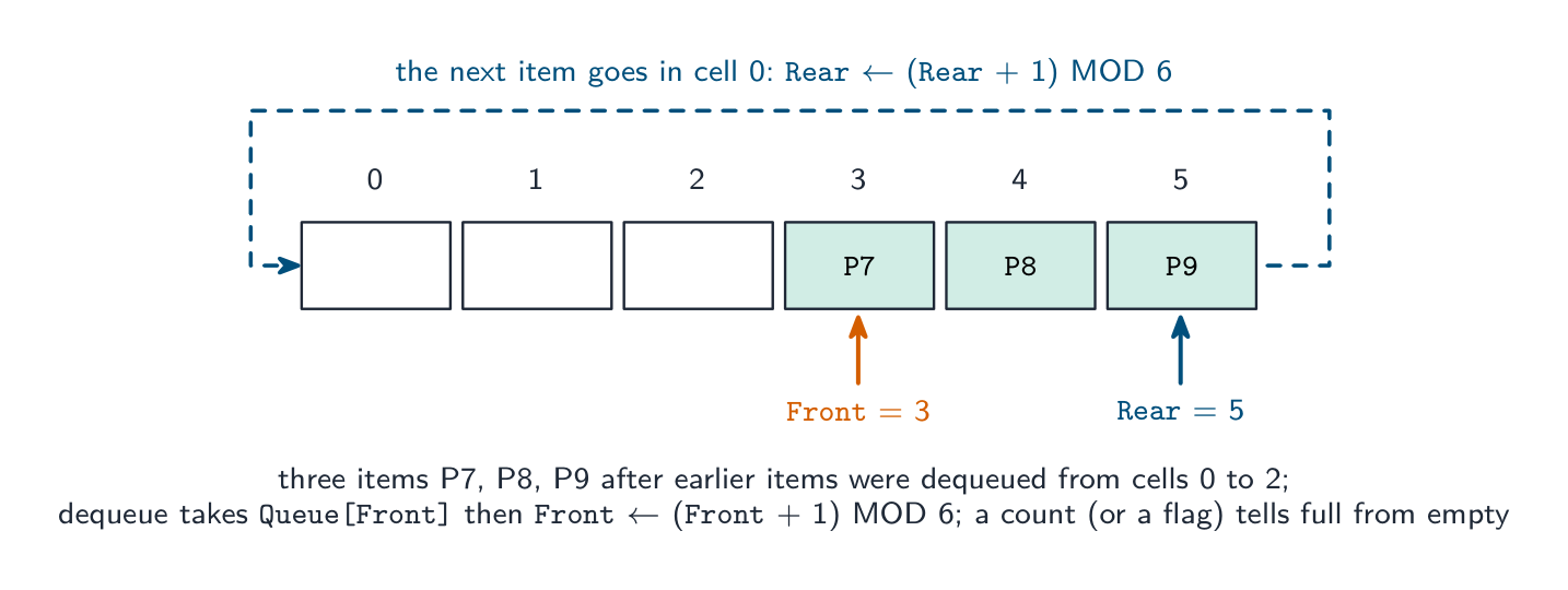
תור (ראשון נכנס, ראשון יוצא): פריטים מצטרפים ב-סוף (enqueue) ועוברים מה-תחלה (dequeue); שתי איشارות ומספר. בתור ליניארי איشارת התחלה זוחלת לאורך הארגון עד שהמקום בתחלה מבוזבז; תור מעגלי עוטף את שתי האיشارות בעזרת MOD, כך שכל תא מושבש.
תור מעגלי: איشارות האחור והקדמת צועדות קדימה באמצעות MOD, כך שתאי המעריך הראשונים מושבים מחדש ברגע שהפריטים שלהם יצאו
FUNCTION Enqueue(Item : STRING) RETURNS BOOLEAN
    IF Count = 6 THEN      // full
        RETURN FALSE
    ENDIF
    Rear ← (Rear + 1) MOD 6
    QueueArray[Rear] ← Item
    Count ← Count + 1
    RETURN TRUE
ENDFUNCTION
FUNCTION Dequeue() RETURNS STRING
    IF Count = 0 THEN      // empty
        RETURN ""
    ENDIF
    DECLARE Item : STRING
    Item ← QueueArray[Front]
    Front ← (Front + 1) MOD 6
    Count ← Count - 1
    RETURN Item
ENDFUNCTION
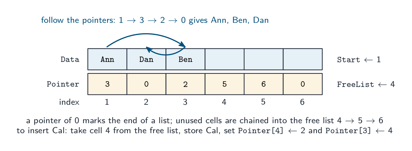
רשימה מקושרת: רצף של צמתים, כל אחד מהם מכיל פריט נתונים ו-איشارה לצומת הבא; איشارת התחלה מציינת את הצומת הראשון ואיشارה null (0 או $-1$) מסתיימת ברשימה. ביישום בעזרת מעריך, שני מערכים מקבילים אחסנו את הנתונים והאיشارות, ותאי שאינם בשימוש מוקשרים ל-רשימת פנויים כדי שהכנסה תדע היכן להניח את הצומת החדש.
רשימה מקושרת בשני מערכים: סדר הרשימה נקבע על ידי האיشارות, ולא על ידי המיקומים; הכנסת שם דורשת לקחת תא מרשימת הפנויים ולחבר מחדש שתי איشارות
FUNCTION FindInList(Target : STRING) RETURNS INTEGER   // index, or 0 if absent
    DECLARE Current : INTEGER
    Current ← Start
    WHILE Current <> 0
        IF Data[Current] = Target THEN
            RETURN Current
        ENDIF
        Current ← Pointer[Current]
    ENDWHILE
    RETURN 0
ENDFUNCTION
כדי להכניס ברשימה מסודרת: קח את התא הפנוי הראשון (NewNode ← FreeList, FreeList ← Pointer[FreeList]), אחסן את הפריט, אז הליך על הרשימה עם איشارת Previous ו-Current עד Data[Current] > Item או לסוף; הגדר את Pointer[NewNode] ← Current ו-Pointer[Previous] ← NewNode (או Start ← NewNode אם הוא מגיע ראשון). כדי למחק, חבר מחדל את הצומת הקודם מעבר לצומת שנמחק וחזר את התא לרשימת הפנויים.
עץ בינארי: צומת שורש, כל צומת מכיל נתונים, איشاره שמאלית לעץ משנה של ערכים קטנים יותר ואיشاره ימינית לעץ משנה של ערכים גדולים יותר. מיושם כמערך ⟨2⟩-ממדי (או שלושה מערכים ⟨1⟩-ממדי) ⟨Tree[Index, 0..2]⟩ לאיشاره שמאלית, נתונים, איشارה ימינה, עם איشارת שורש ואיشارת הבא הפנוי.
FUNCTION FindInTree(Target : INTEGER) RETURNS INTEGER   // index, or -1
    DECLARE Current : INTEGER
    Current ← Root
    WHILE Current <> -1
        IF Tree[Current, 1] = Target THEN
            RETURN Current
        ENDIF
        IF Target < Tree[Current, 1] THEN
            Current ← Tree[Current, 0]      // go left
        ELSE
            Current ← Tree[Current, 2]      // go right
        ENDIF
    ENDWHILE
    RETURN -1
ENDFUNCTION
כדי להכניס: אחסן את הפריט בצומת הבא-פנוי עם שתי איشارות $-1$; אם העץ ריק, הפוך אותו לשורש; אחרת, הליך מטה מהשורש, שמאל או ימין בהשוואה, עד שהאיشارה שתעקוב אחריה היא $-1$, והגדר את איشارה זו לצומת החדש. ADT ממערכת ADT אחרת: ערימה היא רשימה מקושרת שבה push ו-pop פועלים בשני הקצוות; תור הוא רשימה מקושרת עם איشارת התחלה ואיشارת סוף; ניתן לבנות תור מתוך שתי ערימות (push לערימה אחת, pop מהשנייה, העברת הכל כשהשנייה ריקה); צמתים בעץ בינארי הם רשומות או אובייקטים המקושרים באיشارות, ולכן הוא בנוי מבנייה מקושרת של צמתים. ציין אילו פעולות של ה-ADT החדש מתאימות לפעולות של ה-ADT הישן.
עץ דו-סעיפי: כל צומת מכיל עד שני צאריםשלושה סוגי ביקור בעומק לעץ דו-סעיפי: ביקור קדמי, ביקור פנימי (בסדר ערכים) וביקור אחורי
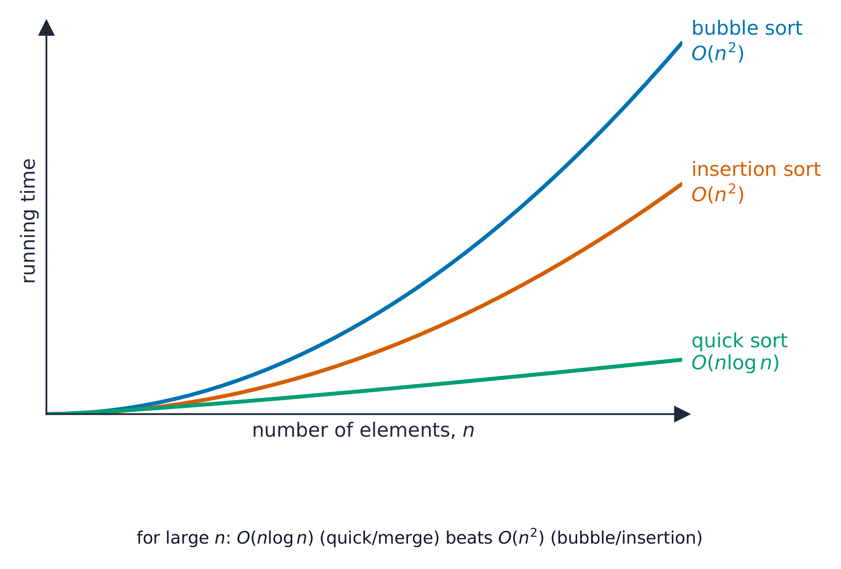
Time complexity 时间复杂度 is how the running time grows with input size $n$, written in Big-O notation 大O表示法 (the dominant term): O(1) constant, O($\log n$) binary search, O($n$) linear search, O($n \log n$) good sorts, O($n^{2}$) bubble/insertion sort. A smaller order is better at scale, even if another algorithm is faster for small $n$.
To make that concrete: to sort a million items, an $O(n \log n)$ sort finishes in a fraction of a second, while an $O(n^{2})$ sort can take minutes.
Worked example. A sorted list holds $1000$ items. How many comparisons does each search need in the worst case?
A linear search checks items one at a time, so it may need up to $1000$ comparisons — this is $O(n)$. A binary search halves the list each step, so it needs at most $\lceil \log_2 1000 \rceil = 10$ comparisons — this is $O(\log n)$. Doubling the list to $2000$ items adds only one comparison to the binary search, but up to another $1000$ to the linear search — which is why the order of growth, not raw speed, decides the winner at scale.
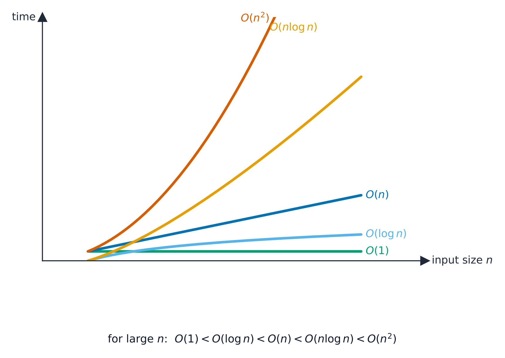
Describing an order.O(1): the time is constant, independent of the number of items (pushing onto a stack, reading an array element). O($\log n$): the time grows with the logarithm of the number of items, so doubling the data adds only a fixed extra step (binary search). O($n$): the time grows in proportion to the number of items (linear search, one pass through a list). O($n \log n$): a little worse than linear (efficient sorts). O($n^{2}$): the time grows with the square of the number of items, so doubling the data quadruples the time (bubble and insertion sort). "State the Big O of a binary search of Names[0:99]" is answered $O(\log n)$, and "describe its meaning" as above; Big O measures how the time or memory scales, not the actual time.
Space complexity
Space complexity 空间复杂度 is the extra memory needed. Bubble and insertion sort use O(1) extra (in place); merge sort uses O($n$); recursion uses stack memory proportional to its depth. There is often a time–memory trade-off.
Other criteria
Simplicity (easier to code and maintain), stability, and adaptiveness (faster on nearly-sorted data). The right algorithm depends on the data and the constraints.
עברית
מורכבות זמנית
מורכבות זמנית היא אופן הגדילת זמן הריצה בהתאם לגודל הקלט $n$, נכתב ב-סימון ביג-או O (האיבר הדומיננטי): O(1) קבוע, O($\log n$) חיפוש בינארי, O($n$) חיפוש ליניארי, O($n \log n$) מיון טוב, O($n^{2}$) מיון בועות/הכנסה. סדר קטן יותר עדיף בקנה מידה גדול, גם אם אלגוריתם אחר מהיר יותר עבור קלט קטן $n$.
כדי להמחיש זאת: כדי למיין מיליון פריטים, מיון $O(n \log n)$ יסתיים בשבר שנייה, בעוד שמיון $O(n^{2})$ עלול לקחת דקות.
דוגמה פתורה. רשימה מסודרת מכילה $1000$ פריטים. כמה השוואות צריך כל חיפוש במקרה הגרוע?
חיפוש ליניארי בודק פריטים אחד אחרי השני, ולכן עשוי לצרוך עד $1000$ השוואות — זהו $O(n)$. חיפוש בינארי חוצה את הרשימה למחצה בכל שלב, ולכן הוא צריך מקסימום $\lceil \log_2 1000 \rceil = 10$ השוואות — זהו $O(\log n)$. הכפלת הרשימה ל-$2000$ פריטים מוסיפה רק שוויה אחת לחיפוש הבינארי, אך עד עוד $1000$ לחיפוש הליניארי — והעובדה הזאת היא שהסדר הגדילה, ולא המהירות הגורסת, קובע את המנצח בקנה מידה גדול.
תיאור סדר גודל.O(1): הזמן הוא קבוע, ללא תלות במספר הפריטים (הוספה לערימה, קריאת אלמנט באייפוס). O($\log n$): הזמן גדל עם הלוגריתם של מספר הפריטים, ולכן הכפלת הנתונים מוסיפה רק שלב נוסף קבוע (חיפוש בינארי). O($n$): הזמן גדל ביחס למספר הפריטים (חיפוש ליניארי, מעבר אחד ברשימה). O($n \log n$): מעט גרוע יותר מליניארי (מיונים יעילים). O($n^{2}$): הזמן גדל עם ריבוע מספר הפריטים, ולכן הכפלת הנתונים מארבעת את הזמן (מיון בועות ומיון הכנסה). "תן את ביג-או של חיפוש בינארי ב-Names[0:99]" התשובה היא $O(\log n)$, ו"תאר את המשמעות" כפי שמתואר למעלה; ביג-או מודד איך הזמן או הזיכרון מתרחבים, לא הזמן האמיתי.
השוואת סדרי הגודל הנפוצים: סדר קטן יותר מנצח בקנה מידה גדולאיך זמן המיון גדל בהתאם למספר האלמנטים $n$: מיונים $O(n^2)$ מתרחקים ממיון $O(n\log n)$
מורכבות מרחב
מורכבות מרחב היא הזיכרון הנוסף הנדרש. מיון בועות ומיון הכנסה משתמשים ב-O(1) נוסף (מיקום); מיון מיזוג משתמש ב-O($n$); רקורסיה משתמשת בזיכרון ערימה פרופורציונלי לעומק שלה. לעיתים קרובות יש קונטרסט בין זמן לזיכרון.
קריטריונים אחרים
פשטות (קל יותר לתכנן ולתחזק), יציבות, ואדפטביות (מהיר יותר על נתונים כמעט מסודרים). האלגוריתם המתאים תלוי בנתונים ובמגבלות.
Explore · חקור
How running time grows with n · כיצד זמן הרצה גדל עם גודל n
Slide n upward and compare the curves: O(1) and O(log n) stay almost flat, O(n) rises steadily, O(n²) explodes. This is why Big-O — not a stopwatch — is how we compare algorithms on large inputs. · הזזו את ציר ה-n כלפי מעלה והשוו בין העקומות: O(1) ו-O(log n) נשארים כמעט שטוחים, O(n) עולה באופן רציף, ו-O(n²) מתפוצץ. זוהי הסיבה לכך ש-Big-O — ולא סופר זמן בפועל — הוא הכלי להשוואת אלגוריתמים על קלט גדול.
Explore · חקור
Big-O growth · גדילת Big-O
Change the input size n and compare how fast each algorithm's work grows — the idea behind time complexity. · שנה את גודל הקלט n והשווה איזה מהאלגוריתמים גדלים מהר יותר — הרעיון מאחורי מורכבות זמן.
19.2
Recursion · רקורסיה
Syllabus · סיילבוס
English
Candidates should be able to:
Notes and guidance
Show understanding of recursion
Essential features of recursion How recursion is expressed in a programming language Write and trace recursive algorithms When the use of recursion is beneficial
Show awareness of what a compiler has to do to translate recursive programming code
Use of stacks and unwinding
עברית
המועמדים צריכים להיות מסוגלים:
הערות והנחיות
להראות הבנה של רקורסיה
תכונות חיוניות של רקורסיה. איך רקורסיה מבטאת בשפת תכנות. כתוב ועקוב אחרי אלגוריתמים רקורסיביים. מתי שימוש ב-רקורסיה הוא יועיל
להראות מודעות למה שמחייב עשות מחשב צ'יפ (compil er) כדי לתרגם רקורסיבי קוד תכנות
שימוש ב-stacks ו-unwinding
Source: Cambridge International syllabus · מקור: הסיילבוס הבינלאומי של קמבריד'ג'
English
Recursion: the call stack winds up and unwinds
Recursive algorithms use recursion 递归: the routine calls itself with a smaller version of the same problem, until a base case 基本情形 ends the chain. It has two parts: the base case (small enough to solve directly — without it the recursion never stops) and the recursive case 递归情形 (reduce the input and call itself).
Factorial 阶乘:
Recursion is natural for self-similar problems: trees, divide-and-conquer 分治 (binary search, merge sort), and nested data. When it is a poor fit, a loop is usually cleaner.
"Describe what is meant by recursion" (two marks).A function or procedure that is defined in terms of itself: it calls itself from within its own body, with a smaller version of the problem each time, until a base case is reached."State three essential features of recursion": (1) a base case (stopping condition) that returns a value without a further call; (2) a general case 一般情形 in which the routine calls itself; (3) each call moves the problem closer to the base case (the parameter is reduced), so that the recursion terminates. Some schemes add: values are returned as the calls unwind.
"Describe when the use of recursion is beneficial, and give an example." When the problem is naturally defined in terms of smaller versions of itself, so that the recursive solution is shorter, clearer and closer to the mathematical definition than a loop would be: a factorial or Fibonacci number, a binary search, traversing a binary tree, merge sort or quicksort, and processing nested structures such as folders within folders. It is a poor choice when the depth is large (the stack may overflow) or when the same sub-problem is computed many times (naive Fibonacci).
Tracing a recursive call
For Factorial(4): the calls go down to Factorial(1)=1, then unwinding multiplies back up: 2*1=2, 3*2=6, 4*6=24. Final result 24. Track each pending call on a stack.
Worked example. The function below is given without an explanation. Trace Unknown(3, 5) and state its output and return value.
Call 1: $X = 3, Y = 5$: $3 < 5$, output 8, call Unknown(4, 4). Call 2: $4 < 4$ is false, return 0. Unwinding: call 1 returns $0 + 1 = 1$. Output 8, return value 1. Write the trace as a table with a row per call (parameters, condition, output, what it returns), and do the returns from the deepest call upwards: that is the unwinding the mark scheme looks for.
Worked example (Fibonacci).Fib(n) returns n when n < 2, otherwise Fib(n - 1) + Fib(n - 2). Find Fib(5).
Fib(5) = Fib(4) + Fib(3); Fib(4) = Fib(3) + Fib(2); Fib(3) = Fib(2) + Fib(1); Fib(2) = Fib(1) + Fib(0) = 1 + 0 = 1. So Fib(3) = 1 + 1 = 2, Fib(4) = 2 + 1 = 3, Fib(5) = 3 + 2 = 5. The base case is reached many times (Fib(2) is computed three times), which is why this version is slow: it makes 15 calls for $n = 5$ and roughly doubles the calls for every increase in $n$.
Converting recursion to iteration. Every recursive routine can be rewritten with a loop, which uses less memory and is faster: keep a running result and loop from the base case upwards. Factorial as a loop:
Asked to change a recursive insertion sort or search into an iterative one, replace the self-call with a loop over the index that the recursion was stepping through, and turn the base case into the loop's exit condition.
Risks
infinite recursion if the base case is missed — crashes with a stack overflow 栈溢出.
high memory use for deep recursion.
slow if it repeats work (naive Fibonacci is exponential — use a loop or memoisation 记忆化).
עברית
רקורסיה: ערימת הקריאות נטמעת ונפתחת
אלגוריתמי רקורסיה משתמשים ברקורסיה: הפונקציה קוראת לעצמה עם גרסה קטנה יותר מאותו בעיה, עד שמקרה בסיס מפסיק את השרשרת. יש שני חלקים: המקרה הבסיסי (קטן מספיק לפתרון ישיר — בלעדיו הרקורסיה לעולם לא תפסיק) והמקרה הרקורסיבי (צמצום הקלט וקריאה לעצמה).
פקטוריאל:
FUNCTION Factorial(n : INTEGER) RETURNS INTEGER
    IF n = 0 OR n = 1 THEN
        RETURN 1
    ELSE
        RETURN n * Factorial(n - 1)
    ENDIF
ENDFUNCTION
חזרה (Recursion) היא טבעית לבעיות בעלות תכונה של חזר-עצמי: עצים, פירוק-ו-כיבוש (חיפוש בינארי, מייף סדר), ומבני נתונים מקושרים. כאשר זו אינה מתאימה, לולאה (Loop) היא בדרך כלל נקייה יותר.
"תאר מה משמעות החזרה" (שתי נקודות).פונקציה או פרוצדורה המוגדרת באמצעות עצמה: היא קוראת לעצמה מתוך הגוף שלה, עם גרסה קטנה יותר של הבעיה בכל פעם, עד שהגיעה למקרה בסיסי."פרט שלוש תכונות הכרחיות לחזרה": (1) מקרה בסיסי (תנאי עצירה) שמחזיר ערך ללא קריאה נוספת; (2) מקרה כללי שבו הפונקציה קוראת לעצמה; (3) כל קריאה מזיזה את הבעיה קרוב יותר למקרה הבסיסי (הפרמטר מצטמצם), כך שהחזרה מסתיימת. שיטות מסוימות מוסיפות: הערכים מוחזרים כאשר הקריאות מתפרקות.
"תאר מתי השימוש בחזרה הוא יעיל, ותן דוגמה." כאשר הבעיה מוגדרת באופן טבעי באמצעות גרסאות קטנות יותר של עצמה, כך שהפתרון הרקורסיבי הוא קצר יותר, ברור יותר וקרוב יותר להגדרה המתמטית מאשר לולאה: פקטוריאל או מספר פיבונאצי, חיפוש בינארי, סיור בעץ בינארי, מיזוג סדר (Merge Sort) או Quicksort, ועיבוד מבנים מקושרים כמו תיקיות בתוך תיקיות. זהו בחירה גרועה כאשר העומק גדול (הסטק עלול להתמלא) או כאשר אותו תת-בעיה מחושבת רבות (פיבונאצי פשוט).
מעקב אחר קריאה רקורסיבית
עבור Factorial(4): הקריאות יורדות לFactorial(1)=1, ואז הפריקה כופלת חזרה כלפי מעלה: 2*1=2, 3*2=6, 4*6=24. התוצאה הסופית 24. יש לעקוב אחר כל קריאה תלויה על גבי סטק.
דוגמה מפורטת. הפונקציה להלן נתונה ללא הסבר. בצע מעקב עבור Unknown(3, 5) ופרט את הפלט והערך ההחזרתי שלה.
FUNCTION Unknown(BYVAL X, BYVAL Y : INTEGER) RETURNS INTEGER
    IF X < Y THEN
        OUTPUT X + Y
        RETURN Unknown(X + 1, Y - 1) + 1
    ELSE
        RETURN 0
    ENDIF
ENDFUNCTION
קריאה 1: $X = 3, Y = 5$: $3 < 5$, פלט 8, קריאה Unknown(4, 4). קריאה 2: $4 < 4$ הוא שגוי, החזר 0. הפריקה: קריאה 1 מחזירה $0 + 1 = 1$. פלט 8, ערך החזרה 1. כתוב את המעקב בטבלה עם שורה לכל קריאה (פרמטרים, תנאי, פלט, מה שהיא מחזירה), ובצע את ההחזרות מהקריאה העמוקה כלפי מעלה: זוהי הפריקה שהפתרון מצפה לה.
דוגמה מפורטת (פיבונאצי).Fib(n) מחזירה n כאשר n < 2, אחרת Fib(n - 1) + Fib(n - 2). מצא Fib(5).
Fib(5) = Fib(4) + Fib(3); Fib(4) = Fib(3) + Fib(2); Fib(3) = Fib(2) + Fib(1); Fib(2) = Fib(1) + Fib(0) = 1 + 0 = 1. לכן Fib(3) = 1 + 1 = 2, Fib(4) = 2 + 1 = 3, Fib(5) = 3 + 2 = 5. מקרה הבסיס מושג רבות (Fib(2) מחושב שלוש פעמים), והסיבה לכך שהגרסה הזו איטית היא she makes 15 קריאות עבור $n = 5$ וכמעט משנה למעלה את מספר הקריאות בכל עלייה ב$n$.
המרת חזרה לאיטרציה. כל פונקציה רקורסיבית ניתנת לכתיבה מחדש באמצעות לולאה, המשמשת זיכרון פחות ומהירה יותר: שמור על תוצאה צוברית וסרק מנקודת הבסיס כלפי מעלה. פקטוריאל כלולאה:
FUNCTION Factorial(N : INTEGER) RETURNS INTEGER
    DECLARE Result, Count : INTEGER
    Result ← 1
    FOR Count ← 2 TO N
        Result ← Result * Count
    NEXT Count
    RETURN Result
ENDFUNCTION
כאשר מבקשים לשנות מיון השחצה רקורסיבי או חיפוש לאלגוריתם איטרטיבי, החלף את הקריאה לעצמה בלולאה על האינדקס שעליו הייתה הרקורסיה הולכת, והמיר את המקרה הבסיסי לתנאי יציאה של הלולאה.
החזרה משתמשת בסטק הקריאות: קריאות דוחפות מסגרות כלפי מטה למקרה הבסיסי, ולאחר מכן ההחזרות מתפרקות כלפי מעלה
סיכונים
חזרה אינסופית אם המקרה הבסיסי מופסד — קריסה עם התמלאות סטק (Stack Overflow).
צריכת זיכרון גבוהה לחזרה עמוקה.
איטיות אם היא חוזרת על עבודה (פיבונאצי פשוט הוא אקספוננצי — יש להשתמש בלולאה או ממוניזציה (Memoisation)).
Explore · חקור
Recursion unwinds from the leaves up · ריקורסיה מתפרקת מהעלים כלפי מעלה
Step through fib(4) in the order the calls actually finish: the leaves (base cases) resolve first, then each parent combines its children. Notice fib(2) is computed twice — that repeated work is why naive recursion is slow. · עבור את fib(4) בסדר שבו הקריאות למעשה נגמרות: העלים (מקרים בסיסיים) נפתרים תחילה, ולאחר מכן כל אב משלב את הילדים שלו. שים לב ש-fib(2) מחושב פעמיים — העבודה המוחזרת הזו היא הסיבה שהריקורסיה פשוטה איטית.
What the compiler does for recursive code · מה המעבד עושה לקוד רקורסיבי
English
Recursion needs each call to have its own copy of its parameters 参数 and local variables 局部变量. The compiler keeps these on the call stack 调用栈. For each call it pushes a stack frame 栈帧 holding the parameters, the local variables, and the return address 返回地址 (where to resume in the caller). When the function returns, the return value is handed back, the frame is popped, and control resumes at the return address.
Because each call has its own frame, recursive calls don't trample each other's variables. The stack can grow large for deep recursion, which is why very deep recursion may overflow it. This is the same call-and-return mechanism used for ordinary (non-recursive) calls — there is no special "recursion mechanism".
"Explain why a stack is suitable for implementing recursion" (three marks). Each recursive call must save its return address, its parameters and its local variables, and the calls are completed in the reverse order to that in which they were made (the last call made is the first to finish), which is exactly the last in, first out behaviour of a stack: each new call pushes a frame, and each return pops the most recent frame, restoring the caller's state and telling it where to continue. This is the compiler's job when it translates recursive code: it generates the push of a stack frame on every call and the pop on every return, and the frames are unwound as the results come back.
עברית
חזרה דורשת לקריאה כלשהי להיות לה עותק משלה של הפרמטרים והמשתנים המקומיים. המעבד שומר אותם על סטק הקריאות. עבור כל קריאה הוא דוחף מסגרת סטק המכילה את הפרמטרים, המשתנים המקומיים, ואת כתובת ההחזרה (איפה להמשיך בקורא). כאשר הפונקציה מחזירה, ערך ההחזרה מועבר, המסגרת נשלפת, והשליטה ממשיכה בכתובת ההחזרה.
מכיוון שכל קריאה יש לה מסגרת משלה, קריאות רקורסיביות אינן פוגעות במשתנים של אחת מהן. הסטק יכול לגדול מאוד בחזרה עמוקה, וזוהי הסיבה שחזרה עמוקה מדי עלולה למלא אותו. זהו אותו מנגנון קריאה-ו-החזרה המשמש לקריאות רגילות (לא רקורסיביות) — אין "מנגנון חזרה" מיוחד.
"הסבר מדוע ערימה מתאימה ליישום רקורסיה" (שלוש נקודות). כל קריאה רקורסיבית חייבת שמור את כתובת החזרה, הנתונים שלה ואת המשתנים המקומיים, והקריאות מסתימות בסדר הפוך לסדר בהן נעשו (הקריאה האחרונה שנעשתה היא הראשונה להסתיים), שזה בדיוק ההתנהגות של אחרון נכנס, ראשון יוצא של ערימה: כל קריאה חדשה מדחפת מסגרת, וכל חזרה מורידה את המסגרת האחרונה, ומשחזרת את מצב הקורא ומציגה לו היכן להמשיך. זוהי המשימה של המترجم כשהוא תרגם קוד רקורסיבי: הוא מייצר דחיפה של מסגרת ערימה בכל קריאה והורדה בכל חזרה, והמסגרות מתפרקות ככל שהתוצאות חוזרות.
19.2
Definitions the examiner accepts · הגדרות מקובלות בקורס
English
A definition question is marked against fixed wording. Learn these exactly, and give one answer only.
Term
Definition
linear search
checking each item in turn from the start until the target is found or the end is reached
binary search
repeatedly comparing the target with the middle item of a sorted list and discarding the half that cannot contain it
bubble sort
repeatedly passing through the list, swapping adjacent items that are in the wrong order, until a pass makes no swaps
insertion sort
taking each item in turn and inserting it into its correct place among the items already sorted
abstract data type
a collection of data and the operations that can be performed on it, defined independently of how it is stored
stack
a last-in-first-out structure with push and pop at the top
queue
a first-in-first-out structure with items added at the rear and removed from the front
linked list
a sequence of nodes, each holding data and a pointer to the next node, with a start pointer
binary tree
nodes each holding data and pointers to a left subtree of smaller values and a right subtree of larger values
Big O notation
a way of classifying the time (or memory) an algorithm needs by how it grows with the size of the input
recursion
a routine that calls itself with a smaller version of the problem until a base case stops the calls
base case
the condition under which a recursive routine returns without calling itself
unwinding
the returns of a chain of recursive calls, from the deepest call back to the first, as the stack frames are popped
עברית
שאלת הגדרה מוקדמת לפי טקסט קבוע. לימודן במדויק, ותן תשובה אחת בלבד.
מונח
הגדרה
חיפוש ליניארי
בדיקה של כל פריט ברצף מהתחלה עד שמצאים את המטרה או מגיעים לסוף
חיפוש בינארי
השוואה חוזרת של המטרה לפריט האמצעי של רשימה מסודרת והשלכה של המחצית שאינה יכולה להכילה
בסייסון בועה
מעבר חוזר הרצף, החלפת פריטים שכנים הנמצאים בסדר שגוי, עד שמעבר אחד לא מבצע החלפות
בסייסון הכנסה
לקיחת כל פריט ברצף והכנסתו למקומו הנכון בקרב הפריטים שמסודרים כבר
סוג נתונים抽象
אוסף של נתונים והפעולות שניתן לבצע עליהן, מוגדר באופן עצמאי מאופן האחסון שלו
ערימה
מבנה אחרון נכנס, ראשון יוצא עם דחיפה והורדה בחלק העליון
תור
מבנה ראשון נכנס, ראשון יוצא עם הוספת פריטים באחור והסרתם מקדמה
רשימה מקושרת
רצף של צמתים, כל אחד מכיל נתונים ושקע לצומת הבא, עם שקע התחלה
עץ דו-סעיפי
צמתים המכילים נתונים ושקעים לענף שמאלי של ערכים קטנים וענף ימני של ערכים גדולים
סימון Big O
דרך למיון זמן (או זיכרון) שאלגוריתם זקוק לו על פי גודל הגידול שלו עם גודל הקלט
רקורסיה
פונקציה הקוראת לעצמה עם גרסה קטנה יותר של הבעיה עד שמקרה בסיס מפסיק את הקריאות
מקרה בסיס
התנאי שבו פונקציה רקורסיבית חוזרת ללא קריאה לעצמה
פירוק
החזרת ערכי שרשרת של קריאות רקורסיביות, מהקריאה העמוקה ביותר חזרה לקריאה הראשונה, כאשר מסגרות הסטק נמחקים
19.2
Exam tips · טיפים לבחינות
English
Searches: linear needs no order and O($n$); binary needs a sorted array, halves each time and is O($\log n$). Know both algorithms by heart, including the bounds and the flag.
Sorts: bubble with a swapped flag, insertion with a key that shifts larger items right; both O($n^{2}$) worst, O($n$) on sorted data. Performance depends on the number of items and how ordered they are.
ADT implementations are pointer bookkeeping: a top pointer; front, rear and count with MOD; start, pointers and a free list; root with left and right pointers. Always check for full and empty.
Big O is about scaling: constant, logarithmic, linear, square. Say "doubling the data adds one comparison" for a binary search.
Recursion: base case, general case, progress towards the base case; beneficial when the problem is defined in terms of itself; a stack holds the return addresses and variables because calls return in reverse order. Trace with a table and unwind from the deepest call.
Common mistakes
Using a binary search on unsorted data, or on a linked list; and setting Lower ← Mid instead of Mid + 1, which loops for ever.
A bubble sort inner loop that runs to the end of the array every pass, or a swap without a temporary variable.
A push or enqueue that does not test for full, or a pop or dequeue that does not test for empty.
Moving the queue's front pointer without MOD in a circular queue, or treating front = rear as always meaning empty.
Inserting into a linked list by shifting the array contents; only the pointers change.
A recursive function with no base case, or one whose recursive call does not make the problem smaller.
Tracing a recursive call but forgetting to add the pending work on the way back up.
Answering "why a stack" with "because it is fast"; the reason is the last-in-first-out order of the returns.
עברית
חיפוש: ליניארי אינו דורש סדר ו-O($n$); בינארי דורש מיון ומחלק למחצית בכל פעילה והוא O($\log n$). יש לדעת את שני האלגוריתמים בעל-כח, כולל הגבולות והדגל.
מיונים: בועה עם דגל לשינוי, הזרעה עם מקדיש שמזיז פריטים גדולים ימינה; שניהם O($n^{2}$) בחמורה, O($n$) על נתונים ממוינים. הביצועים תלויים במספר הפריטים ובמידת המיון שלהם.
מימוש ADT הוא טיפול באמצעיות: מצביע על הקצה; קדמה, אחורה וספירה עם MOD; התחלה, מצביעים ורשימת חופשיים; שורש עם מצביעים שמאלה וימינה. תמיד לבדוק אם המבנה מלא או ריק.
Big O עוסק בקנה מידה: קבוע, לוגריتمي, ליניארי, ריבועי. ניתן להגיד "הכפלת הנתונים מוסיפה השוואה אחת" עבור חיפוש בינארי.
רקורסיה: מקרה בסיס, מקרה כללי, התקדמות לעבר המקרה הבסיס; מועיל כאשר הבעיה מוגדרת בתלות עצמה; סטק מחזיק כתובות החזרה ומשתנים מכיוון שהקריאות חוזרות בסדר הפוך. מעקב מתבצע בטבלה ופירוק מתחיל מהקריאה העמוקה ביותר.
טעויות נפוצות
שימוש בחיפוש בינארי על נתונים לא ממוינים, או ברשימה מקושרת; וגם הגדרת Lower ← Mid במקום Mid + 1, שיצור לופ אינסופי.
לולאת פנימית של מיון בועות המרצת עד סוף המערך בכל מעבר, או החלפה ללא משתנה זמנית.
הזרקה (push) או הכנסה לתור (enqueue) שאינה בודקת אם המבנה מלא, או פריקה (pop) או יציאה מתור (dequeue) שאינה בודקת אם הוא ריק.
הזזת איחורי החזית (front pointer) של התור ללא שימוש בפונקציית MOD בתור מעגלי, או התייחסות לכך ש- front = rear תמיד משמעותו ריק.
הכנסה לרשימה מקושרת על ידי הזזת תוכן המערך; רק השערים (pointers) משתנים.
פונקציה רקורסיבית ללא מקרה בסיס, או אחת שהקריאה הרקורסיבית שלה לא מקטינה את הבעיה.
מעקב אחר קריאה רקורסיבית אך שכחת להוסיף את העבודה המתוקפלת בעת החזרה למעלה.
מענה לשאלה "מדוע ערימה" עם "כי היא מהירה"; הסיבה היא סדר הפינויים Last-In-First-Out.
Pick one and the site follows you — notes, papers, videos and practice all open on it. · בחרו נושא אחד והאתר יעקוב אחריו — הערות, מסמכים, וידאו ותרגולים פתוחים בו.
Type to search notes, lessons, code, vocabulary and past-paper questions across every subject. · הקלד כדי לחפש הערות, שיעורים, קוד, אוצר מילים ושאלות מבחנים בכל הנושאים.