What this course is, and how to use it
This is the sixth course in University Business: managerial accounting 管理会计 — the numbers managers use to decide: what a product costs, what volume breaks even, what a budget commits, which variances to chase, and which costs a decision actually changes. Course 2's financial accounting reported to strangers; this course arms insiders.
The running case is Nimbus Kitchen, the founders' frozen-meals venture: £6.50 meals, £3.10 variable cost, £4,200 monthly fixed cost. Every unit works the same sheet forward — behaviour, volume, costing, budgets, variances, decisions — and every worked example's numbers are machine-verified.
- Units 6.1–6.2 build the model: how costs behave, and how volume turns contribution into profit.
- Units 6.3–6.5 run the firm: costing systems, the budget set, variance analysis.
- Unit 6.6 closes with decisions: which numbers a choice actually changes.
How to read each unit: the question first, then the machinery, then two escalating worked examples, the mistakes people actually make, and a three-line summary.
Cost behaviour
Why it matters. Every managerial number downstream — break-even, product cost, variances, outsourcing — assumes a cost model. Get the behaviour wrong and the arithmetic is right about the wrong world.
The idea, with a picture. Nimbus Kitchen's monthly cost: £1.20 variable per meal (ingredients and packaging), £2,400 kitchen rent (fixed 固定成本 at any volume in the lease's range), and a supervisor at £1,800 stepping to £2,700 past 6,000 meals. The relevant range 相关范围 is the band where each behaviour claim holds.
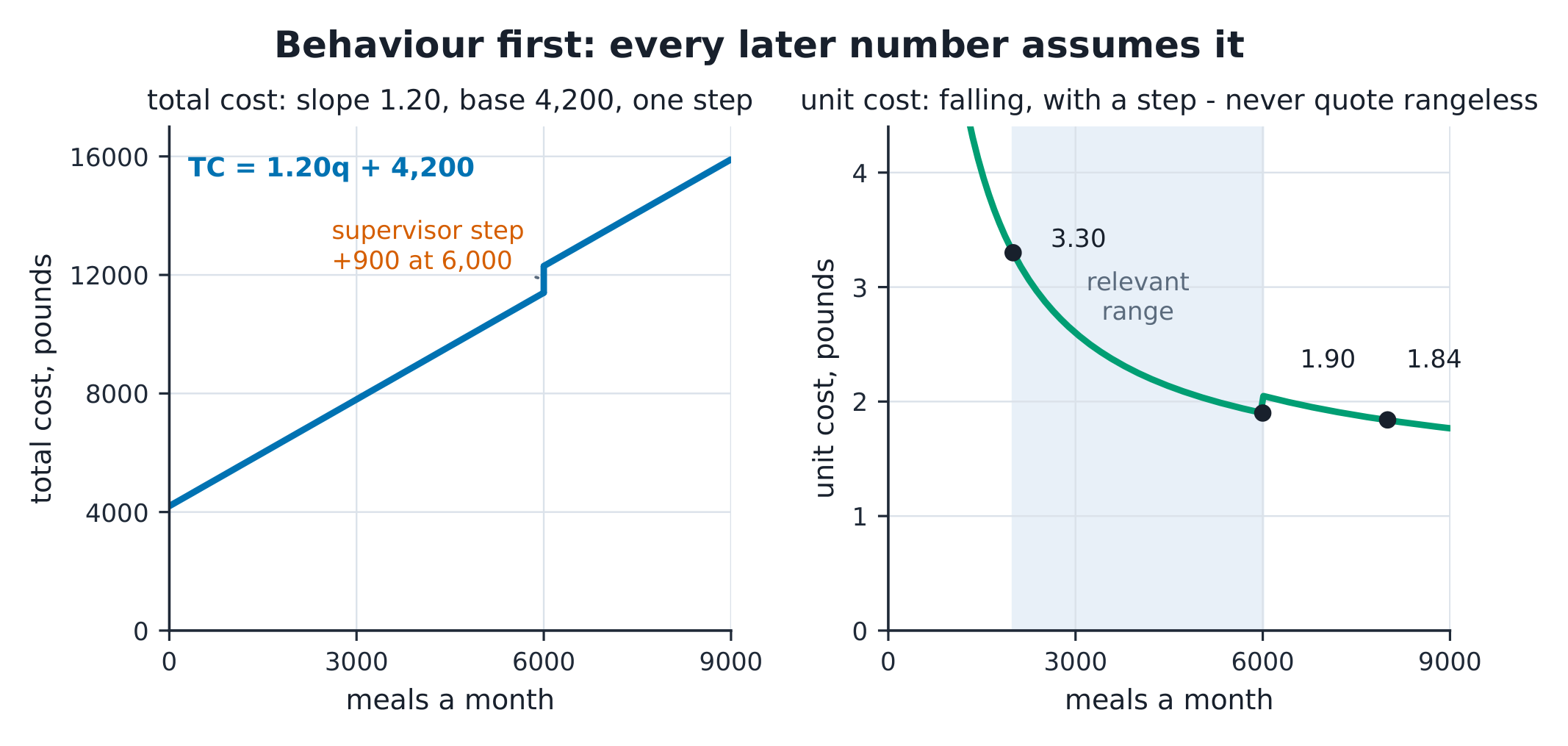
The definitions. Variable cost 变动成本 changes with volume (£1.20/meal); fixed cost does not, within the range (£2,400); step costs jump at thresholds. Mixed costs have both parts. Traceability: direct costs attach to one product; indirect (overhead) costs need allocation — unit 6.3's business.
The derivation. Total cost $= 1.20q + 4{,}200$ up to 6,000 meals, then $1.20q + 5{,}100$: at 2,000 meals £6,600 ✓, at 6,000 £11,400 ✓, at 8,000 £14,700 ✓. Unit cost: £3.30 at 2,000 falling to £1.84 at 8,000 ✓ — the fixed £4,200 spreads over more meals. The high-low estimate on 2,000–6,000 (within one step) recovers exactly £1.20/meal ✓; blind across the step (2,000–8,000) it returns £1.35 — a step cost laundered into a variable one.
Worked example 1 — estimate the function honestly. Four months of data: (2,400, £7,080), (3,300, £8,160), (4,500, £9,600), (5,200, £10,440). High-low: $(10{,}440 - 7{,}080)/(5{,}200 - 2{,}400) = £1.20$ per meal ✓, fixed $7{,}080 - 1.20 \times 2{,}400 = £4{,}200$ ✓. A scatter inspection confirms linearity within the range — the estimate is not just arithmetic, it is an assumption you checked.
Worked example 2 — escalate to the step. July plans 6,400 meals. June's £4,200 fixed no longer holds: the supervisor steps (+£900), so fixed becomes £5,100 and total $= 1.20 \times 6{,}400 + 5{,}100 = £12{,}780$ ✓. The unit cost quoted to retail partners must say WHICH range: £1.98 at 6,400 meals, not June's £2.03-at-3,000 arithmetic blindly extrapolated. Behaviour statements expire at thresholds — date them like milk.
Common mistakes. Quoting unit fixed costs as if they were costs of one more unit (marginal cost is £1.20, not £1.90). Extrapolating a cost function past its relevant range. And treating step costs as either purely fixed or purely variable because the spreadsheet prefers it.
Summary. $TC = vq + F$ within the range; steps break the range. Marginal cost is v; unit cost is $v + F/q$ — different animals.
Cost-volume-profit analysis
Why it matters. "How many meals to break even?" "What volume for £5,000 profit?" "What if the price falls 5%?" CVP is the manager's flight simulator, and its one big simplification — linear behaviour in the relevant range — is also its licence.
The idea, with a picture. At £6.50 a meal with £3.10 variable, the contribution margin 边际贡献 is £3.40 per meal (52.3% of price). Fixed costs of £4,200 need $4{,}200/3.40 = 1{,}235$ meals — the break-even point 保本点, £8,029 of sales.
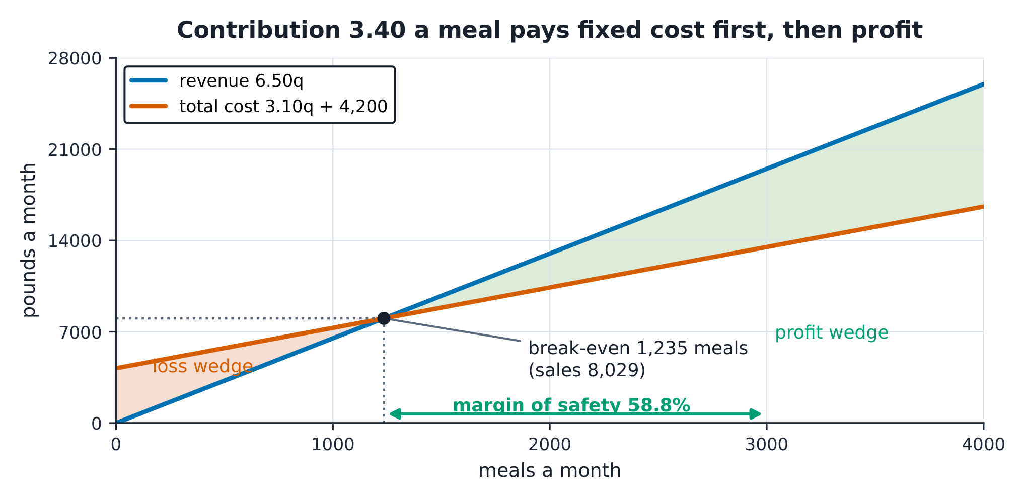
The definitions. $CM = P - v$; CM ratio $= CM/P$. Break-even: $q^* = F/CM$. Margin of safety 安全边际: $(q_{plan} - q^*)/q_{plan}$. Operating leverage 经营杠杆: $CM/\text{profit}$ — how hard profit swings with volume.
The derivation. Profit $= CM \cdot q - F$: at 3,000 meals, $3.40 \times 3{,}000 - 4{,}200 = £6{,}000$ ✓. Break-even $1{,}235$ meals ✓ (check: $1{,}235 \times 6.50 = £8{,}028$ sales, cost $= 1{,}235 \times 3.10 + 4{,}200 = £8{,}029$ — within rounding ✓). Target profit £5,000: $q = (4{,}200 + 5{,}000)/3.40 = 2{,}706$ meals ✓. Margin of safety at the 3,000-meal plan: $1{,}765/3{,}000 = 58.8$% ✓.
Worked example 1 — target profit with tax. The founders want £6,000 AFTER a 25% tax: pre-tax profit must be $6{,}000/0.75 = £8{,}000$, so $q = (4{,}200 + 8{,}000)/3.40 = 3{,}588$ meals ✓. The tax rate enters only through the profit target — divide, then proceed. Check the sanity of the answer against capacity: at 3,588 meals the kitchen is within the 6,000-meal step ✓ — the CVP world still holds.
Worked example 2 — escalate to the mix. Two meals: Alpha at £5.00 (CM £2.60) and Beta at £4.00 (CM £1.80), sold 60:40. The bundle: price $0.6 \times 5.00 + 0.4 \times 4.00 = £4.60$, CM $= 0.6 \times 2.60 + 0.4 \times 1.80 = £2.28$ ✓. Bundle break-even: $4{,}200/2.28 = 1{,}842$ bundles $=$ 1,105 Alpha + 737 Beta ✓. Now the trap: if the mix drifts to 50:50, the bundle CM FALLS to $0.5 \times 2.60 + 0.5 \times 1.80 = £2.20$ — because Beta carries the lower margin, a mix shift toward Beta lowers the bundle CM and raises break-even. Mix is a margin in disguise: state it, then watch it.
Common mistakes. Using unit cost (with fixed spread) in CVP instead of the variable cost. Forgetting the step when the plan crosses a threshold. And quoting break-even without the mix that produced it.
Summary. $q^* = F/CM$; target profit divides by CM after tax adjustment; mix shifts move the bundle CM — the silent variable.
Costing systems
Why it matters. "What does one meal cost?" has three answers — variable, absorption, and the job-order price — and each answers a different question. Choosing the costing system is choosing which question the number answers.
The idea, with a picture. Direct costs trace (ingredients £1.20, direct labour £1.10 per meal); overhead 制造费用 — variable £0.80 per meal plus the £4,200 fixed block — needs a driver. At normal capacity 4,200 meals (2,100 direct labour hours at 0.5 h/meal), the pool is $0.80 \times 4{,}200 + 4{,}200 = £7{,}560$ → £3.60 per labour hour.
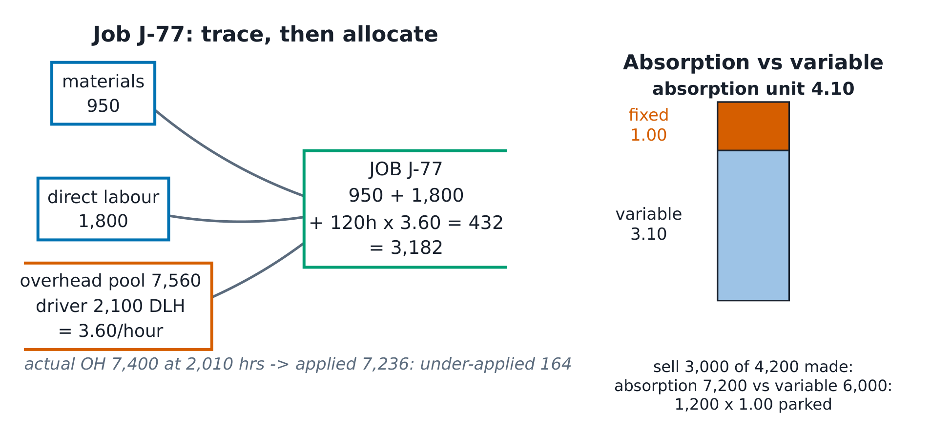
The definitions. Job costing 分批法: costs attach to a unit or batch (the catered order J-77). Process costing 分步法: costs average over continuous production (the meal lines). Absorption vs variable costing: absorption includes fixed overhead in unit cost (here £4,200/4,200 = £1.00 per meal); variable expenses it. Over/under-applied: the gap between applied and actual overhead.
The derivation. Job J-77 (a 120-hour catering batch): materials £950 + direct labour £1,800 + overhead $120 \times £3.60 = £432$ → £3,182 ✓. If the month's actual overhead is £7,400 at 2,010 actual hours (4,020 meals × 0.5), applied is $2{,}010 \times 3.60 = £7{,}236$ → under-applied by £164 ✓ — the rate's estimate was low, and the costing income statement must reconcile it.
Worked example 1 — absorption vs variable income. Produce 4,200 (normal capacity — so no volume variance), sell 3,000, close 1,200. Absorption unit cost $= 3.10 + 1.00 = £4.10$; absorption profit $= 3{,}000 \times (6.50 - 4.10) = £7{,}200$; variable profit $= 3{,}000 \times 3.40 - 4{,}200 = £6{,}000$ ✓ — the £1,200 gap is exactly the 1,200 unsold meals × £1.00 of fixed cost parked in inventory. Production inflates absorption profit: know which arrow you are reading.
Worked example 2 — escalate to the driver choice. Overhead is really 60% machine-driven. A single labour-hour rate loads the hand-finished Alpha line with the automation's cost. Two pools: machine-driven £4,536 (60% of £7,560) over 1,800 machine hours → £2.52/hr; the remaining £3,024 over 2,100 labour hours → £1.44/hr ✓. Job J-77 (120 labour hours, 0 machine hours) falls from £432 to £173 of overhead — the costing system just changed the product's apparent profitability. Drivers are not plumbing; they are pricing decisions about who pays for capacity.
Common mistakes. Reconciling over/under-applied overhead by ignoring it. Reading absorption profit as performance when inventory moved. And choosing drivers by data availability alone — convenience costing is still an allocation with an attitude.
Summary. Trace direct, allocate indirect through a stated driver. Absorption parks fixed cost in inventory; variable exposes it. The driver decides who pays.
Budgeting
Why it matters. A budget is a plan with numbers that commits spending, coordinates departments, and — like any target — changes the behaviour of the people measured by it.
The idea, with a picture. The operating budget set 预算 builds left to right: sales budget → production budget → direct materials and overhead → cash budget. Nimbus Kitchen plans May–July sales of 3,200 / 3,600 / 4,000 meals at £6.50.
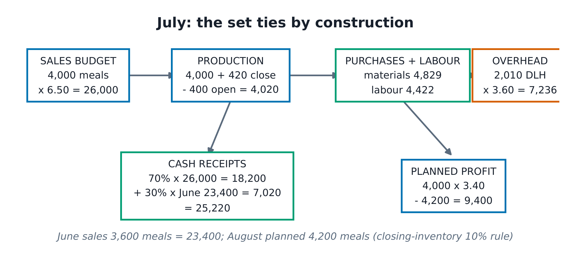
The definitions. The production budget: sales + closing inventory − opening inventory. The cash budget converts sales to receipts by collection pattern (70% in month, 30% following). Flexible budgets restate plans at actual volume for variance work (unit 6.5). Budget slack and gaming are behavioural facts, not errors.
The derivation. July production: sales 4,000 + closing inventory (10% of August's 4,200 = 420) − opening (10% of July = 400) = 4,020 meals ✓. July cash receipts: 70% of July sales ($0.7 \times 4{,}000 \times 6.50 = £18{,}200$) + 30% of June ($0.3 \times 3{,}600 \times 6.50 = £7{,}020$) = £25,220 ✓. The profit budget ties back to CVP: July's planned profit $= 4{,}000 \times 3.40 - 4{,}200 = £9{,}400$ ✓.
Worked example 1 — the set ties. Build July's purchases: production 4,020 meals × £1.20 materials = £4,824; materials inventory at 5% of next month (August 4,100 meals × £1.20 × 5% = £246 closing; opening 5% of July = £241) → purchases £4,829 ✓. Direct labour £1.10 × 4,020 = £4,422; overhead applied at 2,010 hours × £3.60 = £7,236 — inside which sits the £4,200 fixed block. Every figure consumes another's output; change the sales plan and the whole sheet breathes. That coupling is the point.
Worked example 2 — escalate to behaviour. The production manager is bonused on hitting the 4,020-meal budget. August demand collapses to 3,700. The honest flexible budget says 3,730 production (3,700 + 370 − 340); the manager's incentive says overproduce toward 4,020 to "hit target", parking £1.00/meal of fixed cost in inventory (unit 6.3's absorption trap) and reporting profit the cash cannot find. The budget's arithmetic was never wrong — the target was. Participative budgets and rolling reforecasts exist precisely because plans and incentives drift.
Common mistakes. Budgeting production as sales (inventory policy disappears). Treating the cash budget as the profit budget with a lag — timing and measure differ. And evaluating volume-variance performance against a budget nobody re-based after the world moved.
Summary. The set ties: sales → production → purchases/labout/overhead → cash. Inventory and collection policies are the hinges. Budgets shape behaviour as surely as they record it.
Variance analysis
Why it matters. The budget said £2.40/kg of flour at 0.25 kg per meal; July said otherwise. Variances decompose the gap into price, usage and volume pieces, each with an owner — the antidote to "costs were up".
The idea, with a picture. July: 4,020 meals produced, 1,050 kg of flour used (standard: $4{,}020 \times 0.25 = 1{,}005$ kg), paid £2.50/kg (standard £2.40). The flexible budget 弹性预算 restates the plan at 4,020 meals; the variances measure the rest.

The definitions. Each variance 差异 compares actual with standard: the usage variance is $(AQ - SQ) \times SP$, the price variance is $(AP - SP) \times AQ$; and a favourable variance 有利差异 means below-standard cost or above-standard revenue — not "good": a favourable price variance from lower-grade flour can buy an adverse usage variance plus a quality problem. Volume variances compare actual and budgeted activity.
The derivation. Usage: $(1{,}050 - 1{,}005) \times 2.40 = £108$ adverse ✓ — the kitchen used 45 kg more than the standard allows. Price: $(2.50 - 2.40) \times 1{,}050 = £105$ adverse ✓ — the buyer paid 10p over. Total materials variance: £213 adverse ✓, and the two leaves sum exactly to it — the decomposition is an identity, not an opinion.
Worked example 1 — who owns what. The £108 usage variance belongs to the kitchen (yield, training, recipe drift); the £105 price variance to purchasing (supplier, timing, grade). A manager folding them into one number owns nothing and learns nothing. And the two can trade: the buyer's cheaper flour (favourable price) thickens the sauce (adverse usage). Variances are a conversation between centres, and the tree is the agenda.
Worked example 2 — escalate to honest interpretation. Sales volume variance for July: actual 3,700 meals against the 4,000 budget at CM £3.40 → £1,020 adverse ✓. But a supplier strike took the kitchen down for three days; the flexible-budget revenue cost of those days is roughly £2,550 of contribution — the "variance" is mostly a diagnosis, not a performance. Three questions before judging any variance: is it material (a £12 rounding variance is not a finding), is it controllable by its owner, and is it offset elsewhere (a favourable price buying an adverse usage)? Variances start inquiries; they do not end them.
Common mistakes. Computing variances against the STATIC budget when volume moved (the flexible budget is the baseline). Summing variances into one number and delegating it to nobody. And reading favourable as virtue — cheap can be expensive.
Summary. Usage × standard price; price gap × actual quantity; the leaves sum to the total. Every leaf has an owner; every owner gets the conversation, not the verdict.
Relevant-cost decisions
Why it matters. The special order arrives at £3.60 against a £6.50 list price, the outsourcer bids £4.40 against a £4.10 absorption cost, and the sunk machine sits there whispering. Decisions need only the numbers that CHANGE — and the discipline to ignore the rest.
The idea, with a picture. A relevant cost 相关成本 is one that differs between the alternatives: always future, always differential. Sunk costs never qualify; allocated fixed costs rarely do.

The definitions. Sunk cost 沉没成本: already incurred, ignores you. Avoidable cost: disappears with the decision. Opportunity cost: the best alternative forgone. The decision rule: compare incremental revenue against incremental cost, including opportunity.
The derivation. The special order: 800 meals of idle capacity, offer £3.60. Relevant cost per meal: variable £3.10 + £0.15 special packaging = £3.25 → contribution £0.35 × 800 = £280, accept ✓. The £4.10 absorption unit cost is irrelevant — most of it is fixed cost that exists either way, plus an allocation with an attitude.
Worked example 1 — outsourcing with a freed cost. A co-packer bids £4.40 per meal against Nimbus's £4.10 absorption cost. Looks like "buy" — but only £3.10 of the internal cost is avoidable, plus £0.30 of rent actually freed by shutting one kitchen line: avoidable £3.40 < £4.40 → keep making ✓. The remaining £0.70 per meal is fixed or allocated — the decision does not change it, so the decision does not consult it. Every outsourcing bid is really two questions: what truly disappears, and what could the freed space earn instead?
Worked example 2 — escalate to product mix. Flour is short: 1,020 kg available against next month's 4,040-meal plan (1,010 kg) — a 10 kg squeeze, or with Alpha needing 0.30 kg and Beta 0.20 kg, the real question is which meal earns more per kg of flour. Alpha: CM £2.60 / 0.30 kg = £8.67/kg; Beta: £1.80 / 0.20 = £9.00/kg — Beta earns more per scarce kg, so in a true constraint, bias the mix toward Beta and let Alpha wait ✓. General rule: rank products by CM per unit of the BINDING constraint, not per unit of product. Constraints move; the ranking discipline travels.
Common mistakes. Letting sunk costs argue ("we've spent too much to stop now"). Absorption unit costs masquerading as decision costs. Forgetting opportunity costs of freed capacity — zero is an assumption, not a law.
Summary. Relevant = future + differential. Sunk never, allocation rarely, opportunity always. Rank by CM per binding constraint.