What this course is, and how to use it
This is the third course in University Business: microeconomics 微观经济学原理 — the study of how people and firms choose under scarcity, and how those choices meet in markets. The subject is a pair of habits, not a pile of curves: state the assumption before using a model, and check the incentive before predicting a response. Every diagram in this handout is paired with the algebra behind it, and every worked example is machine-verified — the equilibrium, the elasticity, the cost table and the welfare triangle all recompute exactly as printed.
The running case stays with Nimbus Bakery Ltd and its city. The market is artisan bread: daily demand and supply curves for a loaf, then Nimbus's own ovens and bakers as the production story, then the city's market structure, and finally the flour mill upstream whose smoke makes the textbook's market failure concrete. One set of numbers runs through all six units — the £4 loaf you derive in unit 3.2 is the price Nimbus takes as given in unit 3.5.
- Units 3.1–3.3 build the market: choice, demand and supply, elasticity.
- Units 3.4–3.5 go inside the firm: costs, then pricing by market structure.
- Unit 3.6 asks when the market answer is wrong — and what intervention can and cannot repair.
How to read each unit: a story first, then a picture, then precise definitions, then two escalating worked examples whose numbers are machine-verified, the mistakes people actually make, and a three-line summary.
Scarcity and opportunity cost
Why it matters. Nimbus has 12 baker-hours a day and two products that compete for them. Everything microeconomics will say later rests on this one situation: to choose anything is to give something up, and the cost of a choice is the best alternative it displaces — not the money, the alternative.
The idea, with a picture. The production possibilities frontier 生产可能性边界 draws every combination of celebration cakes and sandwich loaves the 12 hours can produce, given the bakery's recipes and skill. Points on the curve use everything; points inside waste time; points beyond need more hours or better skill. The curve bows outward because bakers are not identical: the first cake is made by the baker best at cakes, the last cake would have to be made by someone brilliant at loaves.

The definitions. Scarcity 稀缺 means wants exceed resources at any moment. Opportunity cost 机会成本 is the value of the next-best alternative given up — the loaf hours, not the flour bill. A model's ceteris paribus 其他条件不变 clause ("all else equal") is a promise about what is being held fixed, and every prediction in this course inherits it.
The derivation. With 6 loaves per hour, loaves = 6 × hours left after cakes. Cake hours rise with skill mismatch, so the frontier through the five verified points (cakes, loaves) = (0, 72), (1, 66), (2, 58), (3, 47), (4, 30), (5, 0): each extra cake gives up 6, then 8, then 11, then 17, then 30 loaves — increasing opportunity cost, which is the same statement as the outward bow.
Worked example 1 — the second cake. Nimbus currently bakes one cake a day. The festival asks for a second. The cost is not flour and butter; it is 8 loaves — the hours the second-best cake baker would have spent at 6 loaves an hour. Priced at £4 a loaf, the second cake's opportunity cost is £32, and it is worth baking only if the cake sells for more than £32 plus its ingredient bill. The decision rule generalises: expand until marginal benefit equals opportunity cost.
Worked example 2 — escalate to growth. The council offers a training grant that lifts every baker to 7 loaves an hour. The frontier shifts out to (0, 84), (1, 77), (2, 68), (3, 56), (4, 35), (5, 0) — check the first segment: giving up 7 loaves, not 6. Growth does not remove scarcity: the curve still binds, choices still trade off, and the opportunity cost of cake number 3 has risen from 11 loaves to 12. What changed is the menu, not the necessity of choosing.
Common mistakes. Counting the money spent instead of the alternative forgone (the flour was bought either way — sunk). Drawing a straight-line frontier and then talking about increasing cost — a straight frontier has constant cost. And reading "efficiency" as one point: every point ON the curve is efficient; which one is best depends on the customer, not the curve.
Summary. Cost = next-best alternative, not cash out. The frontier's slope is opportunity cost; the bow is increasing cost. Growth shifts the menu; choice remains.
Demand and supply
Why it matters. The city's artisan-bread market is where Nimbus's £4 loaf comes from. Demand and supply is a machine with three parts — two curves and their interaction — and almost every microeconomic question is a comparative statics exercise on it: shift one curve, recompute, compare.
The idea, with a picture. Daily demand for artisan loaves is $Q_d = 1200 - 100P$; daily supply is $Q_s = 400 + 100P$ (prices in £). The curves cross once: at £4, buyers take 800 loaves and bakers offer exactly 800. Below £4 the plans conflict — buyers want more than bakers will bake — and the shortage bids the price up; above £4 a surplus pushes it down. The crossing is the only price where nobody has an incentive to change behaviour.

The definitions. Demand 需求 is the whole relationship between price and quantity buyers plan to buy; quantity demanded 需求量 is one point on it. A price change MOVES ALONG the curve; anything else that shifts buyer plans (income, tastes, other prices, expectations) SHIFTS the curve — the two vocabulary errors this unit exists to kill. Supply 供给 and quantity supplied 供给量 split the same way for sellers. Equilibrium 均衡 is the price where plans agree; comparative statics 比较静态 is the discipline of changing one thing, holding the rest, and comparing equilibria.
The derivation. Set $Q_d = Q_s$: $1200 - 100P = 400 + 100P$, so $800 = 200P$ and $P^* = £4$, $Q^* = 800$. The same algebra finds any new equilibrium after a shift — and the shortage at £2 ($Q_d - Q_s = 1200-200 - (400+200) = 400$ loaves) and the surplus at £6 (also 400 the other way) come from the same two lines.
Worked example 1 — the festival raises incomes. A week-long festival lifts city incomes; at every price buyers now want 200 more loaves, so demand becomes $Q_d = 1400 - 100P$. New equilibrium: $1400 - 100P = 400 + 100P$ gives $P^* = £5$, $Q^* = 900$ — both price and quantity rise, which is the signature of a demand shift outward along an upward supply. Nimbus, watching its till, sees the £1 without needing to know why — the market aggregated the festival for it.
Worked example 2 — escalate to a supply shock. Flour prices fall; at every price bakers offer 200 more loaves: $Q_s = 600 + 100P$. New equilibrium: $1200 - 100P = 600 + 100P$ gives $P^* = £3$, $Q^* = 900$ — quantity rises again but the PRICE now falls, the signature of a supply shift. The two shocks together (both curves shift right) give $P^* = £4$ again with $Q^* = 1000$: quantities add, price effects cancel — a check students can run in one line before drawing anything.
Common mistakes. Saying "demand rose so the demand curve shifted up" and then ALSO moving along it — pick one mechanism per event. Confusing a shift of supply with a movement along supply caused by the new price. And predicting quantity without the second curve: neither curve alone pins down an equilibrium.
Summary. Price changes move along; other changes shift. Equilibrium solves two equations. Each single-curve shock moves price and quantity in its own signature direction.
Elasticity
Why it matters. Direction is not enough. When the festival pushed the price to £5, Nimbus's revenue ROSE — but a taxi firm raising fares the same 25% might lose revenue. Elasticity is the number that tells you which world you are in, and it is the firm's first pricing question.
The idea, with a picture. The price elasticity of demand 需求价格弹性 is the percentage response of quantity to a percentage change in price, $\varepsilon = \frac{\Delta Q / Q}{\Delta P / P}$. On the bread demand at £4: $\varepsilon = (-100 \times 4) / 800 = -0.5$ — quantity responds half as fast as price in percentage terms, so a higher price RAISES revenue: the price gain beats the quantity loss. The revenue rectangles make it visible: at £4 the rectangle is £4 × 800 = £3,200; at £5 it is £5 × 700 = £3,500 — taller and barely narrower.
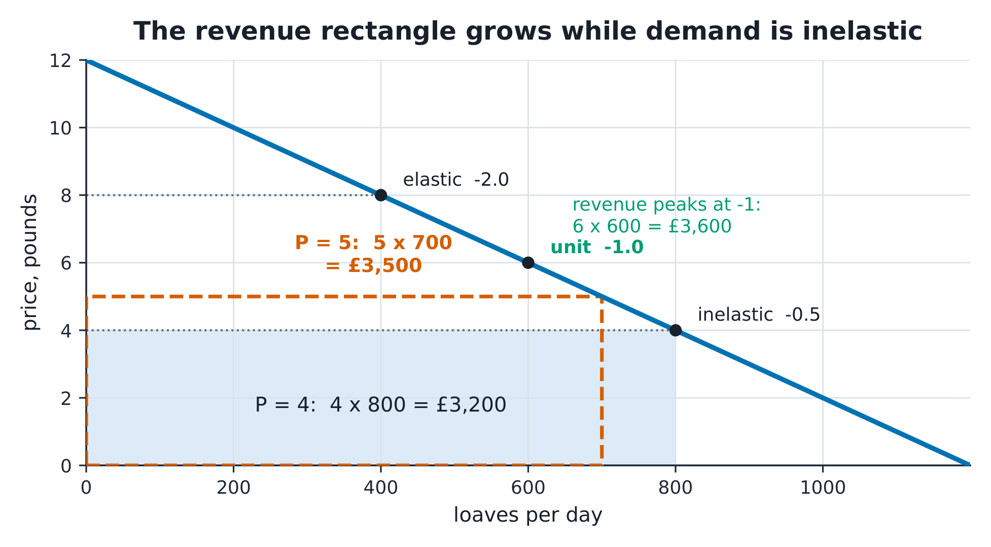
The definitions. Demand is inelastic when $|\varepsilon| < 1$ (quantities respond less than proportionally), elastic when $|\varepsilon| > 1$, unit elastic at exactly 1. On a straight-line demand, elasticity falls from infinity at the top to zero at the bottom — "elastic" and "inelastic" label POINTS, not whole curves. The income elasticity 收入弹性 and cross elasticity 交叉弹性 apply the same machinery to income changes and other goods' prices — they classify goods: normal or inferior, substitutes or complements.
The derivation. For a linear demand $Q = a - bP$, the point elasticity is $\varepsilon = -b \cdot P/Q$. Since $Q$ shrinks as $P$ rises, $|\varepsilon|$ grows along the curve; total revenue $P \cdot Q$ is maximised exactly where $\varepsilon = -1$ (the rectangle can no longer grow) — which is the midpoint of a linear demand. Elasticity is a ratio of percentage changes, so it has no units and can compare bread with taxi rides.
Worked example 1 — the bakery's pricing floor test. At £4, $\varepsilon = -0.5$; at £5, $\varepsilon = -100 \times 5 / 700 = -0.71$ — still inelastic, and revenue indeed rose £3,200 → £3,500. Push to £8: $Q = 400$, $\varepsilon = -2.0$ — elastic, and revenue falls to £3,200 again. The revenue-maximising price sits where $\varepsilon = -1$: $-100P/(1200-100P) = -1$ gives $P = £6$, $Q = 600$, revenue £3,600 — the largest rectangle the demand allows. Elasticity is not a curiosity; it is the pricing dial.
Worked example 2 — escalate to classification. Festival data lets Nimbus classify its neighbours. Incomes rise 10% (from £4,000 to £4,400 a month) and bread quantity rises 15% (800 → 920): income elasticity $= 0.15/0.10 = 1.5$ — a normal good, expenditure-share LUXURY. Then the bread price moves £4 → £5 and the croissant stall's quantity falls 200 → 160: midpoint cross elasticity $= (-40/180) / (1/4.5) = -1.0$ — complements, and strongly so. Three elasticities, three business decisions: price, target customers, and what to bundle.
Common mistakes. Using slope instead of elasticity (slope depends on units; elasticity does not). Quoting "the elasticity of demand" as a single number for a whole linear curve. And forgetting the sign convention: demand elasticity is negative; saying "elasticity is 0.5" without the minus is how price predictions flip.
Summary. $\varepsilon = -bP/Q$ on a linear demand; revenue rises with price while inelastic, peaks at $-1$, falls when elastic. Income and cross elasticities classify goods into normal/luxury and substitute/complement.
Production and costs
Why it matters. To explain Nimbus's supply behaviour in the next unit you need its cost structure — and costs come from production, not from an accountant's spreadsheet. One production table generates every cost curve in the textbook, and the connections between them are the unit's real content.
The idea, with a picture. Nimbus's day: ovens cost £200 whatever happens (the fixed cost 固定成本), each baker is paid £90, and output per baker falls as the small shop fills: with 1–10 bakers the daily loaves are 100, 190, 270, 340, 400, 450, 490, 520, 540, 550. The marginal product 边际产量 of successive bakers is 100, 90, 80, … — diminishing returns 边际报酬递减, the physical law behind every rising marginal cost curve.

The definitions. Variable cost 可变成本 changes with output (here wages: $90L$); total cost adds the fixed £200. Marginal cost 边际成本 is the cost of one more loaf: $MC = w / MPL$ — the wage divided by what the last baker adds. Average total cost 平均总成本 is cost per loaf, $ATC = (90L + 200)/Q$. Economies of scale 规模经济 describe the LONG run, when the shop itself can grow — do not confuse falling ATC from spreading a fixed cost with scale economies.
The derivation. The table is exact by construction: at $L = 5$, $Q = 400$, $MC = 90/60 = £1.50$, $AVC = 450/400 = £1.125$, $ATC = 650/400 = £1.625$; at $L = 8$, $Q = 520$, $MC = 90/30 = £3.00$, $ATC = £1.77$. Two structural facts follow from the arithmetic alone: MC rises because MPL falls, and MC cuts ATC at ATC's minimum (about £1.63 at $Q = 400$) — when the marginal loaf costs less than the average, the average falls, and vice versa: the grade-point-average logic.
Worked example 1 — the ninth baker. The eighth baker adds 30 loaves (£3.00 each against the £4 market price — worth it). The ninth adds 20 loaves at £4 = £80 of revenue for £90 of wage: marginal cost $90/20 = £4.50 > £4$. Nimbus stops at eight bakers, 520 loaves, profit $4 \times 520 - (90 \times 8 + 200) = 2080 - 920 = £1{,}160$. The rule "produce while $MC \le P$" and the rule "hire while the baker's value exceeds the wage" are the same sentence.
Worked example 2 — escalate to the shutdown question. A supermarket price war drops the loaf to £0.85. That is below the smallest average variable cost on the table — £0.90, the first baker's 100 loaves at £90 of wages — so no scale of baking even pays the bakers who do it: the best candidate, one baker, brings £85 of revenue against £90 of wages. Shut the ovens for the price war's duration and lose only the £200 fixed cost. The boundary is worth one more look: had the price settled at £1.00, the answer flips — the first 190 loaves cover their £180 of wages and £10 of the rent, so bake with two bakers and lose £190 rather than £200. Produce when $P \ge \min AVC$; when $P < \min AVC$, every loaf deepens the loss.
Common mistakes. Treating fixed cost as irrelevant to decisions (it is irrelevant to the MARGINAL decision — and decisive for the shutdown one). Averaging first and differencing after (MC comes from the marginal product, never from a change in ATC). And reading scale economies from a falling short-run ATC — the shop never changed size.
Summary. $MC = w/MPL$; diminishing returns make it rise. MC cuts ATC at its minimum. Produce while $P \ge MC$, shut down below min AVC.
Market structures
Why it matters. The same bakery, facing a different market, prices differently — and the city's welfare differs with it. Structure is a spectrum defined by two questions: does the firm face a given price, and can it keep its profits from being competed away?
The idea, with a picture. In perfect competition 完全竞争 each of the city's many bakeries is a price taker at £4: its demand curve is flat, it supplies 520 loaves (unit 3.4's answer), and free entry grinds profit toward zero in the long run. A monopoly 垄断 — one bakery with the whole market and a blocked entry — faces the market demand curve and chooses the point on it that maximises profit: $Q = 500$, £7 a loaf. Between them sit monopolistic competition 垄断竞争 (many sellers, differentiated loaves, free entry — Nimbus's actual world) and oligopoly 寡头垄断 (few sellers whose prices depend on each other's choices).

The definitions. A firm's market power is measured by the Lerner index $(P - MC)/P$ — zero for a price taker. The monopolist sets marginal revenue equal to marginal cost and charges the demand price of that quantity; because it faces the whole downward demand, $MR$ lies below the price. The deadweight loss 无谓损失 is the trades between $Q_m$ and the efficient quantity that mutually beneficial exchange would have made but the markup priced out.
The derivation. Market demand inverted is $P = 12 - Q/100$, so revenue is $TR = 12Q - Q^2/100$ and $MR = 12 - Q/50$. With the industry's marginal cost flat at £2 (a simplification — the point here is the markup rule, not the cost shape), $MR = MC$ gives $12 - Q/50 = 2$, so $Q_m = 500$ and $P_m = 12 - 5 = £7$. Lerner index $(7-2)/7 = 0.71$. At the competitive benchmark of this diagram, $P = MC = £2$ would sell $Q = 1000$, so the markup kills the trades from loaf 500 to loaf 1000 — a deadweight loss of $\tfrac{1}{2}(7 - 2)(1000 - 500) = £1{,}250$ a day against this cost curve.
Worked example 1 — the canal concession. Suppose Nimbus buys every rival and the council grants the towpath concession exclusively. Setting $MR = MC$: 500 loaves at £7, revenue £3,500, cost at £2 a loaf £1,000, profit £2,500 — the largest the demand and this cost curve allow. Every buyer between the 500th and the 1,000th loaf values a loaf above its £2 marginal cost but below £7 — those trades die, and their surplus (the £1,250 triangle) is nobody's. The monopoly profit is a transfer; the triangle is a loss.
Worked example 2 — escalate to the real middle. Nimbus's actual market is monopolistic competition: its sourdough is distinct, so it has a small markup — but the festival's profits attract a rival bakery, whose entry shifts Nimbus's own demand curve left until economic profit is zero. The equilibrium condition is not $P = MC$ (differentiation costs that) but $P = ATC$ with $P > MC$ — markup exactly eaten by the cost of variety. Check the logic on the numbers: entry ends when Nimbus's profit £1,160 has been competed to zero, and the customer's choice set has grown by one bakery — the welfare verdict on variety versus markup is a genuine argument, not a formula.
Common mistakes. Saying the monopolist "charges the highest price it can" — it charges the price of its MR = MC quantity, which is well below the top of the demand curve. Reading deadweight loss off the wrong pair of quantities. And treating the four structures as a moral ladder — they are predictions about price and output, evaluated case by case.
Summary. Price taker: $P = MC$, zero long-run profit. Monopolist: $MR = MC$, markup by the Lerner rule, deadweight loss between $Q_m$ and $Q_c$. Monopolistic competition: markup yes, economic profit no.
Market failure and intervention
Why it matters. The flour mill upstream burns cheap coal; the smoke drifts over the city. Every loaf's flour carries a cost nobody's bill shows — and the £4 equilibrium from unit 3.2 quietly over-produces bread relative to what the city actually wants. This unit is about the one situation every market failure shares, and what a tax can and cannot do about it.
The idea, with a picture. An externality 外部性 is a cost or benefit that falls on people outside the transaction. The mill's smoke makes each loaf's true marginal social cost 社会边际成本 exceed the bakers' private supply curve by £1.20 a loaf. The private market clears at £4/800; the social optimum is where demand meets MSC — 740 loaves. The gap between the two quantities is the over-production, and the triangle between demand, supply and MSC over that gap is the social loss.

The definitions. Marginal social cost adds the private marginal cost and the marginal external cost; efficiency requires MSB = MSC. A Pigouvian tax set equal to the external cost re-creates the efficient quantity — the tax wedge 税收楔子 splits the price buyers pay from the price sellers keep. Incidence 归宿 says who really bears a tax: it depends on elasticities, not on who hands over the money. Public goods (non-rival, non-excludable — street lighting) and information failures complete the family of failures a price system cannot price.
The derivation. With the £1.20 external cost, the efficient quantity solves demand against cost-plus-wedge: buyers face $P_c$, sellers keep $P_p = P_c - 1.20$, and $1200 - 100P_c = 400 + 100P_p$ gives $P_c = £4.60$, $P_p = £3.40$, $Q = 740$ — exactly the MSB = MSC quantity. A tax of £1.20 achieves it: revenue £1.20 × 740 = £888, and the burden splits £0.60 to buyers (4 → 4.60) and £0.60 to sellers (4 → 3.40) — the equal split is no accident: the curves' elasticities at the equilibrium match.
Worked example 1 — the smoke, priced. The council prices the mill's damage at £1.20 a loaf's worth of flour. Before: 800 loaves, and loaves 741–800 each cost the city more in smoke damage than they are worth to buyers — check loaf 780: a buyer values it at £4.20 and the baker's private cost is £3.80, which is why the trade happened, but the social cost is £5.00 — the city pays £1.20 that no bill showed. After the £1.20 tax: 740 loaves, buyers pay £4.60, bakers keep £3.40, the mill pays £888 into the clean-air fund, and the damage on the 60 loaves no longer baked never happens. The over-production triangle — roughly $\tfrac{1}{2} \times 1.2 \times 60 = £36$ a day — is the pure gain.
Worked example 2 — escalate to the limits. Now the council tries the same £1.20 as a plain revenue tax with the mill unpriced — same wedge, wrong target: quantity still falls to 740, but the externality is untouched and the £888 buys roads. Intervention matches the failure or misfires. Then the honest second list: the £1.20 damage estimate is a measurement (the true MSC curve is not printed anywhere); enforcement costs eat the £36; and if bakers' supply were perfectly inelastic the entire wedge would land on sellers regardless of the paperwork. State the model, state its limits — the unit's last lesson is about intellectual honesty, not triangles.
Common mistakes. Confusing the tax REVENUE rectangle with a welfare gain — it is a transfer, and the deadweight triangles are the stakes. Assuming the statutory payer bears the incidence — elasticities decide. And concluding "externality, therefore tax": the number has to be measured, and measurement is where most real policies fail.
Summary. MSC = MPC + external cost; efficient quantity sets MSB = MSC. A tax equal to the external cost restores it; incidence follows elasticities. Every intervention claim carries a measurement and its limits.