What this course is, and how to use it
This is the fifth course in University Business: business statistics 商业统计 — the discipline of turning data into decisions without lying to yourself. One reproducible dataset runs the whole course: 40 takeaway delivery times from Nimbus's weekend service, in minutes, with every statistic in this handout recomputable from the data page at the end.
The course's spine is a single habit: state the claim, state the uncertainty, and say what would change your mind. Means carry standard errors; tests carry their assumptions; correlations carry disclaimers; and every worked example's numbers are machine-verified against the dataset.
- Units 5.1–5.2 collect and describe: sampling, bias, honest pictures.
- Units 5.3–5.5 reason under chance: probability, estimation, testing.
- Units 5.6–5.7 relate and decide: regression, correlation, and the limitations that separate analysis from persuasion.
How to read each unit: the question first, then the machinery, then two escalating worked examples, the mistakes people actually make, and a three-line summary.
Data and sampling
Why it matters. Every number in a business report came from SOME selection process. Before you interpret the number, you must know what was selected, how, and who was missed — or the analysis downstream is decorating a guess.
The idea, with a picture. The 40 delivery times are a sample 样本 from the weekday service — all orders in a period would be the population 总体. The sampling design decides what the sample can honestly say: a simple random sample 简单随机样本 gives every order the same chance; convenience samples (the orders the manager happened to see) do not.

The definitions. Data is quantitative (delivery minutes) or categorical (which rider); scales are nominal, ordinal, interval, ratio — minutes are ratio (zero means zero). Bias 偏差 is systematic error from the design: selection bias (who is reachable), non-response bias (who answers), survivorship (who remains). A data dictionary records each field's meaning, unit and coding — reading one critically is step zero of any analysis — the data dictionary 数据字典 is the dataset's passport.
The derivation. Expectations: if the sample is random, the sample mean is an unbiased estimator of the population mean — its long-run average hits the truth. If the design is biased, no sample size rescues it: a convenience sample of 10,000 evening orders still says nothing about lunch. Bias is a property of the DESIGN, not the size.
Worked example 1 — read the dictionary. The dataset's dictionary:
delivery_min (ratio, minutes, one decimal, missing when the rider
forgot to stop the timer — 3 cases); hour (ordinal, 11–21);
rider_id (nominal). Before any average: the 3 missing values are NOT
zero minutes and not random — riders forget more when busy. Decide:
report the mean on the 37 complete cases AND the missingness, never a
silent average.
Worked example 2 — escalate to design. Nimbus wants to know if weekend service is slower. Design A: analyse the 40 times (all from Saturday). Design B: sample 20 Saturday + 20 Wednesday orders — a stratified 分层 sample — because the question compares days. Design A answers "what is Saturday like"; only B answers the question asked. Check the trap in reverse: sampling 20+20 and then pooling into one average weights the days equally whether or not the business does — the design must match the claim, in both directions.
Common mistakes. Treating a convenience sample as random because it is large. Confusing non-response with absence (the customers who did not answer the survey are data). And reading a dataset without its dictionary — units and codings are where analyses die.
Summary. The design is the inference. Bias is systematic and sample size cannot cure it. The dictionary is part of the data.
Descriptive measures and visualisation
Why it matters. "Average delivery: 27.4 minutes" is one sentence that hides a distribution. Description is not a formality before the "real" statistics — it is where most business insight actually lives, and where most business charts lie.
The idea, with a picture. Centre, spread, shape, outliers: the four questions every dataset answers. The 40 times: mean 均值 27.43, median 中位数 27.6, standard deviation 标准差 4.91, quartiles 24.5 / 27.6 / 30.9, IQR 6.3 — and a histogram shows a roughly symmetric single peak with mild right stretch (38.5 is high but within the fence: Q3 + 1.5×IQR = 40.3).
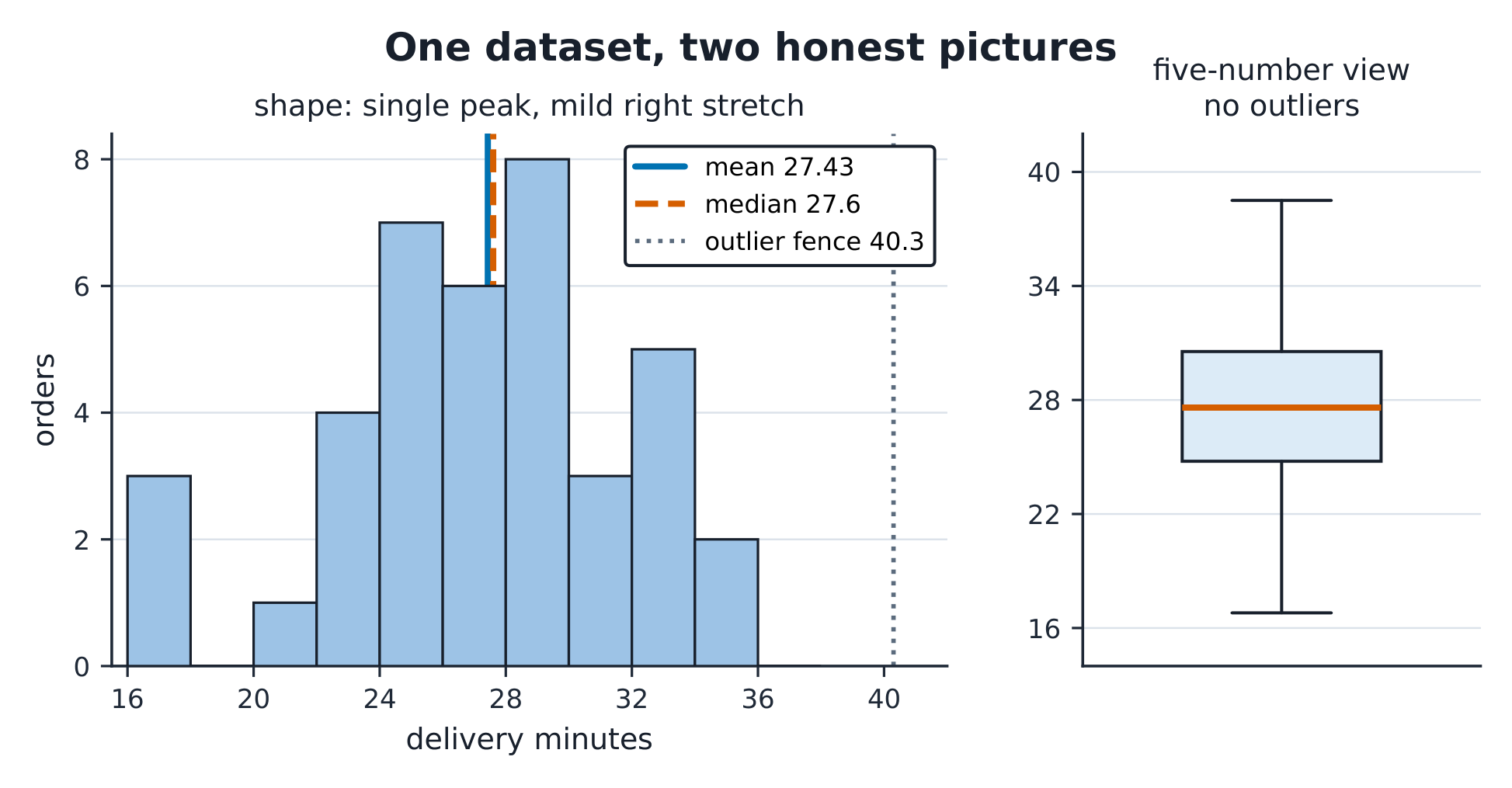
The definitions. Mean = sum/n; median = middle order; sd = $\sqrt{\sum(x_i-\bar x)^2/(n-1)}$; IQR = Q3 − Q1. Outliers: beyond Q1 − 1.5×IQR or Q3 + 1.5×IQR. Shape: symmetric, skewed, multimodal. The mean follows the tail; the median resists it — with a right-skewed income or delay distribution, report the median and say why.
The derivation. For the data: $\bar x = 1{,}097.1/40 = 27.43$ ✓; the sd's numerator is $\sum(x_i-\bar x)^2 = 940.9$, so $s = \sqrt{940.9/39} = 4.91$ ✓. Why divide by $n-1$: the deviations of a sample are constrained ($\sum(x_i - \bar x) = 0$), so $n$ understates spread — one lost degree of freedom, paid to estimate the mean first.
Worked example 1 — the honest picture. A marketing slide shows the delivery chart with a y-axis starting at 24 minutes: the 17–23 minute orders vanish and differences look tripled. Redraw from zero (or a stated broken axis): the 27.4 average sits in an honest landscape. Axis truncation is the oldest lie in the book — the numbers did not change, the picture did.
Worked example 2 — escalate to outliers. Add one data-entry error: a 168-minute delivery (the timer never stopped). New mean: 30.43 (up 2.99 minutes!); new median: 27.65 (up 0.05); new sd: 22.0 (up 17.1). One keystroke moved the mean by 3 minutes and quadrupled the sd, but barely touched the median. Check it against the fence: with the error, Q3 + 1.5×IQR = 46.6 and 168 sits far outside — the fence CATCHES it, and the dictionary explains it. Outlier handling: investigate, document, then decide — never silently delete.
Common mistakes. Quoting a mean for skewed data without saying so. Deleting outliers before investigating them. And choosing chart types by prettiness: a bar chart of a single continuous variable hides everything a histogram shows.
Summary. Centre (mean vs median), spread (sd, IQR), shape, outliers — report all four. The picture can lie even when the numbers are true.
Probability and distributions
Why it matters. "What is the chance this order is late?" is a probability question, and the two workhorse models — binomial and normal — answer most business versions of it. The skill is matching the question to the model and stating why.
The idea, with a picture. If 20% of orders run late, the number of late orders in the next 5 is binomial 二项分布: $P(X{=}2) = \binom{5}{2}(0.2)^2(0.8)^3 = 0.2048$. Delivery times themselves cluster around a centre with symmetric tails — modelled by the normal 正态分布 curve, where 68/95/99.7% of values sit within 1/2/3 sd.
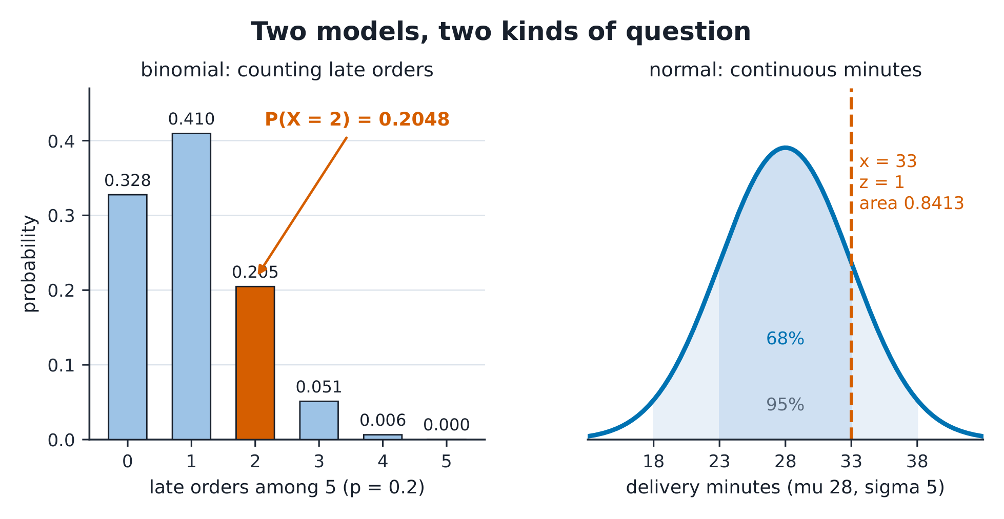
The definitions. Probability rules: $P(A \cup B) = P(A) + P(B) - P(A \cap B)$; independence means $P(A|B) = P(A)$. Binomial: n independent trials, success probability p. Normal: symmetric, bell-shaped, fully described by $\mu$ and $\sigma$. Standardising: $z = (x - \mu)/\sigma$ converts any normal to the standard curve.
The derivation. Binomial probabilities come from counting orders: $\binom{5}{2} = 10$ arrangements × $0.2^2 \times 0.8^3 = 0.02048$ each → 0.2048 ✓; and $P(X \le 1) = 0.8^5 + 5(0.2)(0.8^4) = 0.7373$ ✓. Normal: with $\mu = 28$, $\sigma = 5$, an order at 33 minutes is $z = 1$ above the mean → $\Phi(1) = 0.8413$ below it ✓ — the table's most-used number.
Worked example 1 — the service promise. Nimbus promises "30 minutes or your dessert is free". Under the model $\mu = 28$, $\sigma = 5$: $P(X > 30) = P(z > 0.4) = 1 - 0.6554 = 0.3446$ — a THIRD of orders would claim. At $\mu = 26$: $P(X > 30) = P(z > 0.8) = 0.2119$ still one in five. The promise's cost is a probability statement, and only a faster kitchen (a smaller $\mu$), not a longer promise, changes the tail's shape.
Worked example 2 — escalate to the matching. Three questions, three models — match them. (a) "Of the next 20 orders, chance at least 4 are late (p = 0.2)": binomial, $P(X \ge 4) = 1 - P(X \le 3) = 1 - 0.4114 = 0.5886$. (b) "Chance one order takes over 35 minutes" with $\mu = 28$: normal, $z = 1.4$, tail 0.0808. (c) "Kitchen staff checked 2 of today's 3 Desserts — chance both were the slow ones": counting with combinations, $1/\binom{3}{2} = 1/3$. Wrong model, confidently computed, is still wrong — the justification is part of the arithmetic.
Common mistakes. Adding non-exclusive probabilities without subtracting the overlap. Using the normal for counts (binomial) or skewed delay data without saying so. And reading the table's tail as the body — always draw the curve and shade before you look up.
Summary. Counts → binomial; symmetric continuous → normal; $z = (x-\mu)/\sigma$ is the translation. State the model before computing the number.
Sampling distributions and estimation
Why it matters. The 40 times are one sample; Nimbus could have measured a different Saturday and got a different mean. Estimation is the discipline of saying what the ONE number you have says about the truth you cannot see — with an honest band around it.
The idea, with a picture. Draw a random sample of 16 orders, take its mean; draw again; again — the means themselves form a distribution: narrower than the data, centred on the truth. That is the central limit theorem 中心极限定理, and its width shrinks with $\sqrt{n}$.

The definitions. The standard error 标准误 of the mean is $SE = s/\sqrt{n}$ — the sd of the sample mean, not of the data. A 95% confidence interval 置信区间: $\bar x \pm t \times SE$. The confidence level is a property of the METHOD: 95% of intervals so constructed capture the truth — not "95% probability the truth is in this one".
The derivation. The course's seed-11 random sample of 16 orders: mean 28.66, sd 4.70, so $SE = 4.70/\sqrt{16} = 1.175$. With $t_{15} = 2.131$: the 95% interval is $28.66 \pm 2.50$, i.e. [26.2, 31.2] ✓. Quadruple the sample to 64 and the SE halves — precision is bought at $\sqrt{n}$, the most expensive exchange rate in statistics.
Worked example 1 — read the interval properly. "Average delivery is between 26.2 and 31.2 minutes, 95% confident." Three readings: (a) wrong — "the true mean has a 95% chance of being in [26.2, 31.2]"; (b) wrong — "95% of orders take 26–31 minutes" (that is a prediction interval's job, and it would be far wider); (c) right — "the METHOD that produced this band captures the true mean in 95% of its uses". The interval is about the MEAN, and the confidence is about the PROCEDURE.
Worked example 2 — escalate to the design's limit. The manager wants the mean known to ±0.5 minutes. Required $n$: $t \cdot s/\sqrt{n} \le 0.5$ → $\sqrt{n} \ge 2.131 \times 4.7/0.5 = 20.0$ → $n \ge 401$ orders. One decimal of precision costs ten times the data — and if the sample were convenience-sampled, 401 biased observations are precisely 401 times wrong. Precision and unbiasedness are different purchases.
Common mistakes. Confusing sd (data spread) with SE (mean's uncertainty). Reading the confidence level as a probability about this interval. And forgetting the interval assumes the sampling design was random — the arithmetic cannot repair the design.
Summary. $SE = s/\sqrt{n}$; the CLT makes means roughly normal; $\bar x \pm t \cdot SE$ with the confidence read as a property of the method.
Hypothesis testing
Why it matters. "Is the weekday service actually slower than the weekend?" A test is a formal way to ask whether the data would be surprising if nothing were going on. Used honestly, it disciplines claims; used ritually, it manufactures them.
The idea, with a picture. Set the null hypothesis 零假设 ($H_0$: mean = 30) and its alternative; compute how extreme the sample would be under $H_0$; reject only if the extremeness is past the threshold. The p-value p值: the chance of data at least this extreme IF $H_0$ were true.

A hypothesis test 假设检验 compares the data's extremeness to a chosen threshold. Test statistic $t = (\bar x - \mu_0)/(s/\sqrt n)$. Significance level $\alpha$ — the Type I error rate WE CHOOSE (usually 0.05). Type II error $\beta$ — missing a real effect; power = $1 - \beta$. "Statistically significant" means p < α, no more.
The derivation. Is the mean 30 minutes? With the seed-11 sample: $t = (28.66 - 30)/1.175 = -1.14$. The critical value at α = 0.05, two-sided, 15 df: $|t| > 2.131$. Since $1.14 < 2.131$, we fail to reject — the data are consistent with a 30-minute mean AND with plenty else. Note what this does NOT say: not "the mean is 30", not "there is no difference" — only "this sample would not be surprising if it were".
Worked example 1 — the honest p-value. A rider claims their Saturday route is faster: their 16 runs average 26.9 against the shop's 28.7, $s = 4.0$, so $t = (26.9 - 28.7)/(4.0/4) = -1.8$, p ≈ 0.09. "Almost significant" is not a category — report p = 0.09 and let the decision weigh the cost of being wrong. If free desserts ride on the call, α = 0.10 might be right; if re-training rides on it, 0.05 or 0.01. α is a business choice wearing a Greek letter.
Worked example 2 — escalate to significance vs importance. With n = 400 orders per day, a 0.4-minute difference is p < 0.01 — statistically significant and operationally invisible (no customer notices 24 seconds). With n = 8, a 3-minute difference can be p = 0.3 — invisible to the test yet real to every customer. The fix is not a bigger p-value but a reported EFFECT SIZE with its interval: "0.4 minutes, 95% CI [0.1, 0.7] — significant and trivial". Significance asks "is it there?"; the effect size asks "does it matter?" — business needs the second answer.
Common mistakes. "Accepting" the null (you fail to reject; absence of evidence is not evidence of absence). Confusing p with the probability the hypothesis is true. And p-hacking — testing until something clears 0.05 — which unit 5.7 unpacks.
Summary. $t = (\bar x - \mu_0)/SE$; reject past the threshold chosen as your error budget. p is about the data, not the hypothesis. Significance ≠ importance: always report the effect size.
Regression and correlation
Why it matters. "Do longer deliveries come from farther addresses?" Regression turns pairs of numbers into a line, quantifies how tightly they move together, and — if you are careless — implies a cause. This unit fits the line, reads its residuals, and polices the causal claim.
The idea, with a picture. Twelve tracked deliveries: distance (1.0–3.75 km) and time. The scatter is tight and upward; the least squares 最小二乘 line: $\hat y = 17.4 + 4.83x$ — each extra kilometre costs 4.83 minutes; correlation 相关系数 $r = 0.989$, $r^2 = 0.979$: 97.9% of the variance in time travels with distance.

The definitions. Slope: change in $\hat y$ per unit x; intercept: $\hat y$ at x = 0 (often meaningless — 0 km is not a delivery). Residual 残差: $y - \hat y$, the part the line misses. $r^2$: the share of y-variance the line explains. Extrapolation beyond the data's range is modelling fiction.
The derivation. Least squares minimises $\sum(y_i - a - bx)^2$; the normal equations give $b = r \, s_y/s_x$ and $a = \bar y - b\bar x$. For the 12 deliveries: $b = 4.83$, $a = 17.4$ ✓; residuals run from −1.2 to +1.1 minutes with no pattern ✓ — a straight line is adequate here, and the residual plot is the evidence.
Worked example 1 — read the fit. $\hat y = 17.4 + 4.83x$: a 2 km delivery is predicted $17.4 + 9.7 = 27.1$ minutes; a 3 km one 31.9 ✓. The intercept's 17.4 minutes at 0 km is kitchen+handover time — meaningful here ONLY because the physics suggests a fixed prep component; state such readings, do not inherit them. And a 7 km prediction (51 minutes) is extrapolation: no data beyond 3.75 km has vouched for the line.
Worked example 2 — escalate to the causal police. Correlation of 0.989 is as strong as business data gets — and still proves no direction. Third variables: both distance and time grow with traffic density; the ROUTE assignment (riders take far orders at off-peak) could make distance correlate with time without causing it at the fitted rate. The honest sentence: "distance predicts time in this sample ($r^2 = 0.98$); a causal rate would need route assignment held fixed". Correlation is a statement about THIS dataset's joint variation; causation is a claim about what would change if you intervened — different verbs, different evidence.
Common mistakes. Reading $r^2$ as "99% accurate predictions". Interpreting the intercept when x = 0 is outside meaning. Extrapolating past the data. And the classic: correlation → causation, with no mechanism, no experiment, no caution.
Summary. $\hat y = a + bx$ by least squares; the residuals must be examined, not assumed. $r^2$ measures association; only design earns causation.
Decision limitations
Why it matters. Everything before this unit can be done correctly and still produce a lie — by asking many questions, stopping when convenient, or reporting certainty that never existed. This final unit is the checklist that keeps statistics a discipline instead of a rhetoric.
The idea, with a picture. The traps in a map: multiple testing (20 questions at α = 0.05 expect one "significant" fluke by design: $1 - 0.95^{20} = 0.64$ chance of at least one), stopping rules (peeking at data and continuing until p < 0.05), selection of outcomes (reporting the one metric that moved), and forecast certainty (point predictions without intervals).

The definitions. p-hacking: trying many specifications until one clears the threshold. HARKing: hypothesising after results are known. Publication/selection bias: the file drawer of null results nobody shows you. A forecast without an interval is a mood.
The derivation. Multiple testing arithmetic: 20 independent tests at α = 0.05 → $P(\text{at least one false positive}) = 1 - 0.95^{20} = 0.64$ — a likely fluke, not a discovery. The Bonferroni discipline: for 20 tests at family α = 0.05, each needs p < 0.0025. The 5.5 example now reads both ways: p = 0.09 is "not significant" AND one of the few tests actually reported — the number of unreported tests is part of the number's meaning.
Worked example 1 — the dashboard audit. A dashboard tracks 12 metrics weekly; this week one shows p = 0.04 against last year. Question 1: how many comparisons? 12 metrics × 52 weeks — this "finding" was drawn from a lottery with hundreds of tickets. Question 2: was it declared in advance? No. Question 3: does the effect size matter? 0.3%. Verdict: not evidence of change — evidence of a dashboard's ability to generate headlines. The correct response is a pre-registered confirmation on fresh data.
Worked example 2 — escalate to the honest forecast. The manager forecasts "next Saturday's average delivery: 27.4 minutes". The dataset's answer: the mean of a fresh 40-order Saturday has SE ≈ $4.91/\sqrt{40} = 0.78$, so the forecast should read "27.4 ± 1.5, 95%" — and a single Saturday's average will fall outside that band one time in twenty. Decision consequence: staff to the band's upper end (28.9), not the point. A number without its uncertainty cannot be managed, only hoped at.
Common mistakes. Treating one significant result among many as a finding. Confusing "we failed to reject" with "we proved the null" — the mirror trap of unit 5.5. And demanding certainty from forecasts instead of demanding the interval.
Summary. Count the tests, declare the rules, show the file drawer, band every forecast. Statistics earns decisions by admitting what it does not know.
The dataset (reproducible)
40 takeaway delivery times, minutes, one decimal, sorted:
16.8, 17.2, 17.3, 21.1, 22.8, 22.9, 23.0, 23.0, 24.3, 24.4, 24.9, 25.2, 25.2, 25.2, 25.5, 26.0, 26.1, 26.9, 27.4, 27.5, 27.7, 28.2, 28.4, 28.7, 28.7, 28.9, 28.9, 29.2, 29.3, 30.4, 31.0, 31.4, 32.2, 32.5, 33.2, 33.3, 33.7, 34.8, 35.5, 38.5
Verified statistics: n 40; mean 27.43; median 27.6; sd 4.91; quartiles 24.5 / 27.6 / 30.9; IQR 6.3; no points beyond the 1.5×IQR fences (15.0, 40.3). The estimation sample (seed 11, n = 16): mean 28.66, sd 4.70, SE 1.175, 95% CI [26.2, 31.2], t vs 30 = −1.14. The regression pairs (12 deliveries, km vs minutes): slope 4.83, intercept 17.4, r 0.989, r² 0.979. All figures in this handout recompute from these values.