Binomial Parameters
Introducido| English | Significado |
|---|---|
| parameters/pəˈræmɪtəz/ | parámetros |
The binomial mean
- For a binomial variable, the mean has a beautifully simple formula:
-
$$\mu_X = np$$
- Trials times success-probability — the expected number of successes.
- Flip a coin $100$ times: expect $\mu_X = 100 \times 0.5 = 50$ heads.
The binomial standard deviation
- The standard deviation is:
-
$$\sigma_X = \sqrt{np(1-p)}$$
- It measures how much the count of successes typically varies.
- These two parameters 参数 ($\mu_X$, $\sigma_X$) summarize the whole binomial distribution.
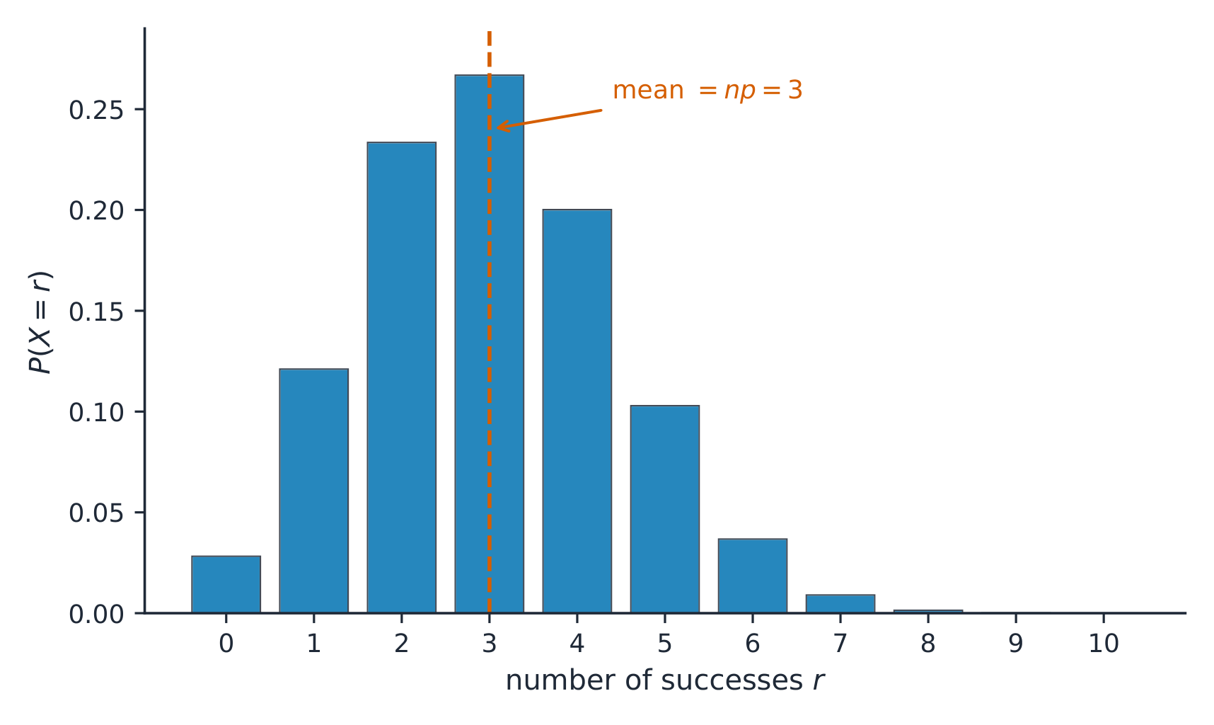
The binomial distribution, with mean n times p
The shape
- For a nondegenerate binomial ($0<p<1$), the shape depends on $p$: at $p=0.5$ it is symmetric.
- $p < 0.5$ → skewed right; $p > 0.5$ → skewed left.
- For fixed $0<p<1$, increasing $n$ makes the distribution more bell-like. Check $np\ge10$ and $n(1-p)\ge10$ before using a normal approximation.
- This near-normal shape for large $n$ powers the inference in later units.
Interpret in context
- Always state the parameters in the problem's own words.
- $\mu_X$: "we expect about $np$ successes on average."
- $\sigma_X$: "the number of successes typically varies by about $\sigma_X$."
- Numbers mean little until tied back to the real situation.
The tidy formulas $\mu=np$ and $\sigma=\sqrt{np(1-p)}$ are for the binomial setting only — don't use them for a general random variable, and only after the BINS conditions check out. And note the SD uses $p(1-p)$: for fixed $n$, it's largest at $p=0.5$ and shrinks as $p$ nears $0$ or $1$ (extreme $p$ makes the count more predictable).
A free-throw shooter takes $n=25$ shots. Assume independent shots with constant success probability $p=0.8$. Let $X$ count makes.
- Mean: $\mu_X = 25 \times 0.8 = 20$ makes expected.
- SD: $\sigma_X = \sqrt{25 \times 0.8 \times 0.2} = \sqrt{4} = 2$.
- Shape: $p=0.8>0.5$ gives left skew. Here $np=20$ but $n(1-p)=5<10$, so the usual large-counts condition for a normal approximation fails.
For a binomial variable, the parameters are $\mu_X = np$ and $\sigma_X = \sqrt{np(1-p)}$. The shape is symmetric at $p=0.5$, skewed otherwise, and more bell-like as $n$ grows. Always interpret $\mu_X$ and $\sigma_X$ in context — expected successes and their typical variation.
Write from a binomial mean of 3
- There are 9 independent trials.
- The success probability is 1/3. The lesson n of 20 is another setting.
A binomial random variable has n=9 independent trials with success probability p=1/3. Find its mean np.
Expected successes are the number of trials times the success probability.
A binomial variable has n=9 and p=1/3. What is its mean np?
Dificultad 1/5 · 100 monedas + un pequeño bono en el primer intento de hoy
9 times 1/3 is 3.
Shape of a binomial distribution
With p ≠ 0.5 the distribution is skewed; larger n looks more bell-like.
A binomial has n = 25, p = 0.8. Find the mean np.
Dificultad 2/5 · 140 monedas + un pequeño bono en el primer intento de hoy
μ = np = 25 × 0.8 = 20.
For n = 25, p = 0.8, find the standard deviation √(np(1−p)).
Dificultad 2/5 · 140 monedas + un pequeño bono en el primer intento de hoy
√(25·0.8·0.2) = √4 = 2.
For a nondegenerate binomial distribution (0<p<1), which value of p gives exact symmetry?
Dificultad 1/5 · 100 monedas + un pequeño bono en el primer intento de hoy
p = 0.5 gives a symmetric distribution.
For a fixed success probability 0<p<1, a binomial distribution becomes more bell-shaped as n grows.
Dificultad 1/5 · 100 monedas + un pequeño bono en el primer intento de hoy
Large n pushes the shape toward normal.
For fixed n, the binomial standard deviation √(np(1−p)) is largest when...
Dificultad 1/5 · 100 monedas + un pequeño bono en el primer intento de hoy
p(1−p) peaks at p = 0.5.