Carrying Out a Goodness-of-Fit Test

The chi-square statistic

• The chi-square statistic 卡方统计量 adds up the standardized gaps across all categories:
• $$\chi^2 = \sum \frac{(\text{observed} - \text{expected})^2}{\text{expected}}$$
• Each term compares one category's observed and expected counts.
• Squaring makes every gap positive; dividing by expected scales it.

Bigger gaps, bigger chi-square

• If observed $\approx$ expected everywhere, each term is tiny → $\chi^2$ is small.
• Large mismatches make terms large → a big $\chi^2$.
• So a large $\chi^2$ is evidence against the claimed distribution.
• $\chi^2$ is always $\ge 0$ (a sum of squares over positives).

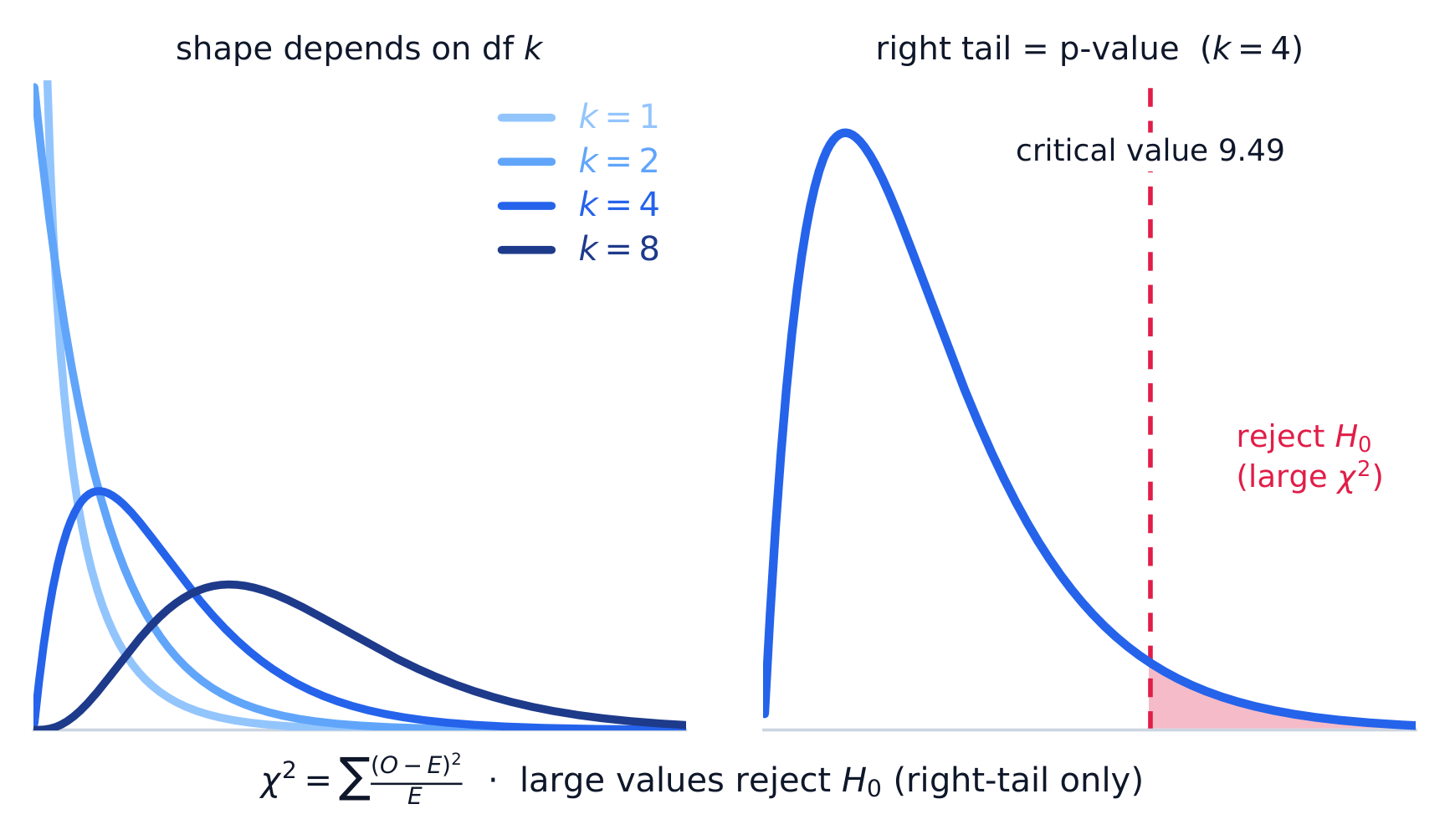
The chi-square distribution: shape depends on df and the p-value is the right tail

Find the p-value

• The p-value is the area to the right of $\chi^2$ under the chi-square curve at the right $df$.
• Chi-square is a right-tailed test — only large values are "extreme."
• A big $\chi^2$ sits far right → small p-value → strong evidence against $H_0$.
• Use technology or a table with $df = \text{categories} - 1$.

Decide and conclude

• Compare the p-value to $\alpha$: p $\le \alpha$ → reject $H_0$; else fail to reject.
• Reject: convincing evidence the true distribution differs from the claim.
• Fail to reject: not convincing evidence against the claimed fit.
• State it in context — about the model's fit to the data.

Write from a contribution of 1.6

• One cell has observed count 14 and expected count 10.
• The lesson contribution 0.4 is another cell.