What this course is, and how to use it
This is the fifth course in University Medicine: human physiology 人体生理学 — how the fabric built in MED03–04 actually runs. Physiology is quantitative medicine: pressures, volumes, clearances and concentrations that you compute, not admire.
Scope limit, stated once: a study course, not a medical degree; every case below is fictional and nothing here licenses or guides treatment.
- Unit 5.1 is the frame: homeostasis as control.
- Units 5.2–5.5 are the great systems: excitation, circulation, respiration, the kidney.
- Units 5.6–5.7 complete the map: gut and hormones.
The medicine habit: every claim is an equation you can evaluate — cardiac output, alveolar gas, clearance, Henderson–Hasselbalch — and every number below is something you recompute.
Homeostasis and body fluids
Why it matters. The body is a controlled system: its whole design goal is keeping the internal environment constant while the outside swings. Learn the control frame once and every later system is an instance of it.
The idea, with a picture. Homeostasis 内环境稳态 = sensor → integrator → effector, in a negative-feedback loop. The body water: total ~42 L in a 70 kg adult — intracellular fluid 细胞内液 28 L (2/3), extracellular fluid 细胞外液 14 L (1/3: plasma 3 L + interstitial 11 L) ✓, separated by selective membranes.

The derivation (why the loop needs a set point). Negative feedback 负反馈 holds a variable near a set point only if the sensor can detect error AND effectors can push both ways. Every physiological control system in this course satisfies that template: baroreceptors sense pressure, the brainstem integrates, heart and vessels effect; chemoreceptors sense CO₂, the medulla integrates, ventilation effects. When you meet a new system, find its three boxes and its set point — the exam question and the clinical failure both live there.
Worked example 1 — the water budget arithmetic. A 70 kg adult: $42\ L = 28$ ICF $+ 14$ ECF $= 28 + 3$ plasma $+ 11$ interstitial ✓. Gain 2 L of water: it distributes by compartment number of particles — ECF (with its sodium) takes $1/3 \approx 0.67$ L, ICF $1.33$ L ✓. The osmolality maths (ECF tonicity governs the split) is the whole of water balance reasoning.
Worked example 2 — clinical link: the failed sensor. (Fictional patient) a steadily low plasma sodium, yet the urine dilutes and concentrates normally around that lower level: the osmostat's set point has been reset low (the reset-osmostat form of SIADH) — the loop runs perfectly, holding the wrong target. Control loops fail three ways: sensor, effector, set point; diagnosis is deciding which.
Common mistakes. Forgetting plasma is part of the ECF. Treating "feedback" as automatically negative (positive feedback exists — clotting, labour — and it drives an event to completion rather than holding a steady state). Counting water intake without metabolic water (~0.3 L/day) or losses through skin and breath (~0.9 L/day).
Summary. 42 L = 28 ICF + 14 ECF (3 plasma + 11 interstitial); sensor-integrator-effector around a set point; water distributes by osmolality; loops fail at sensor, effector or set point.
Excitable cells and muscle
Why it matters. Nerve and muscle speak one electrical language; the action potential 动作电位 is the sentence. Every rhythm you will ever reason about — heartbeat, breathing, peristalsis — is built from it.
The idea, with a picture. Rest: the permeability-weighted (GHK) membrane potential ≈ −70 mV (K⁺ dominates, unit 1.2 of MED01). Excitation: voltage-gated Na⁺ channels open → the upstroke overshoots to +30 mV → Na⁺ inactivates, K⁺ carries the repolarisation → a brief hyperpolarisation, then rest. The absolute refractory period 绝对不应期 (~1 ms in nerve) sets the maximum firing rate ≈ 1000/s ✓.
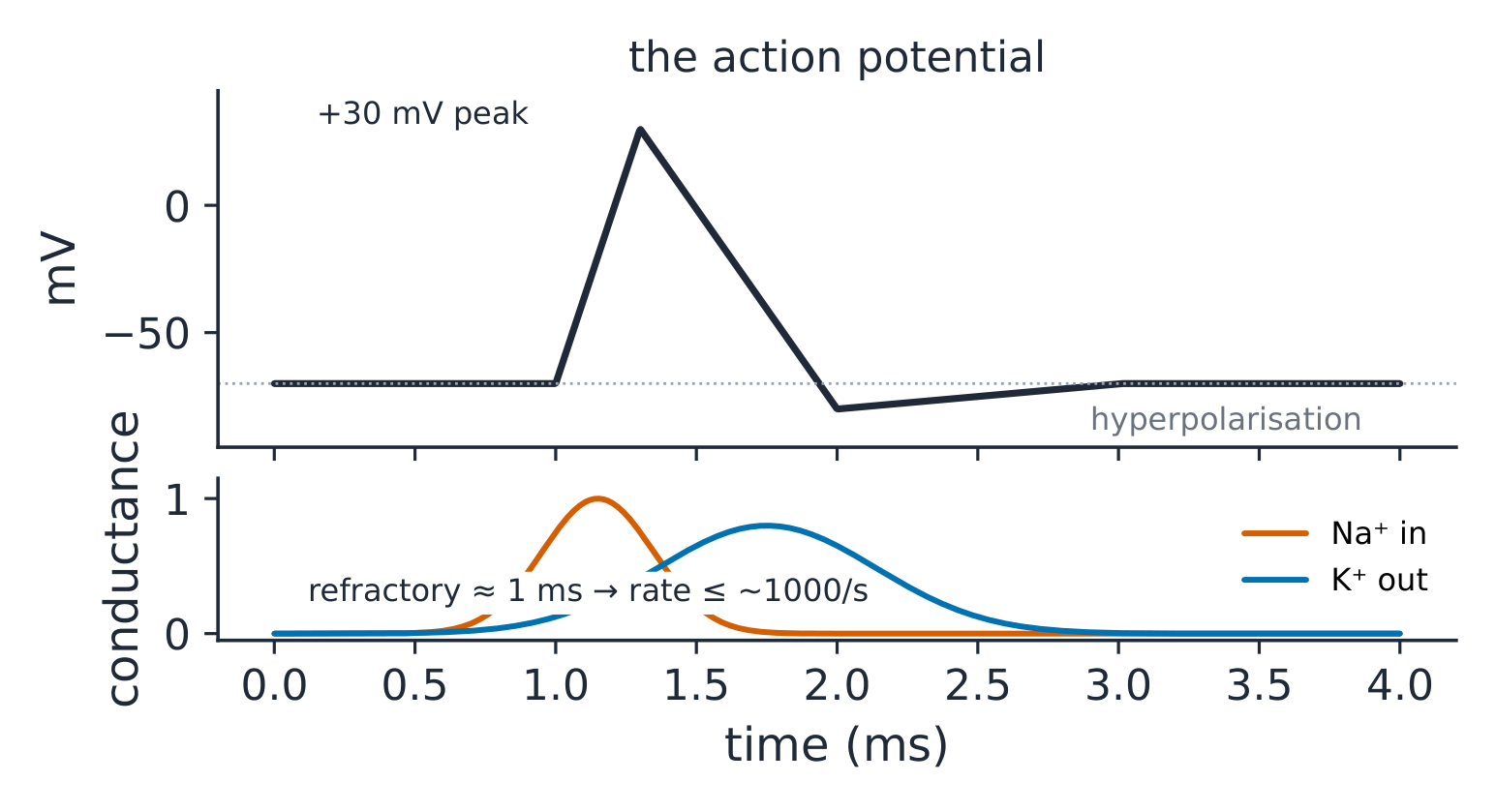
The derivation (why the upstroke is self-reinforcing). Depolarisation opens Na⁺ channels → Na⁺ enters → further depolarisation: positive feedback to the spike. Repolarisation is negative feedback (K⁺). The two loops in sequence explain the all-or-none shape and the threshold: below threshold, K⁺ wins; above it, Na⁺ wins ✓. Propagation is the same event regenerating along the membrane — myelin makes it jump (saltatory conduction 跳跃传导), raising speed from ~1 m/s to up to ~100 m/s ✓.
Worked example 1 — from spike to twitch. In skeletal muscle the spike releases Ca²⁺ from the sarcoplasmic reticulum; Ca²⁺ moves troponin, actin is freed, and the MED04 sarcomere contracts. Summation works because a single twitch (~100 ms) outlasts its refractory (~2 ms): twitches can add. At about 20 stimuli/s they fuse only partly (a bumpy, incomplete tetanus); at about 50/s and above they fuse into tetanus 强直收缩 — smooth, maximal force ✓.
Worked example 2 — clinical link: the channel that fails. (Fictional) periodic paralysis after a carbohydrate meal: insulin drives K⁺ into cells, the extracellular K⁺ falls, and muscle fibres with a faulty channel (a small inward leak) depolarise instead of hyperpolarising; their Na⁺ channels sit inactivated and the fibres cannot fire — a few millivolts in the wrong direction silences a muscle. One ion, one channel, one sentence of mechanism.
Common mistakes. Confusing refractory (no re-firing) with hyperpolarisation (harder to fire). Expecting local anaesthetics to block small pain fibres last (they go FIRST — rate dependence and small-fibre hit). Forgetting cardiac muscle is a functional syncytium via gap junctions — one long refractory prevents tetanus in the heart.
Summary. −70 mV rest; Na⁺ upstroke (positive feedback), K⁺ repolarisation; refractory sets the rate ceiling (~1000/s nerve); myelin → saltatory, up to ~100 m/s; Ca²⁺ couples spike to sarcomere; fast enough stimulation (~50/s) fuses twitches into tetanus — but not in the heart.
Cardiovascular physiology
Why it matters. The circulation is a pump, a set of pipes and a volume — the quantitative heart of medicine. Its three equations (output, resistance, pressure) run every shock, every failure and every blood-pressure clinic.
The idea, with a picture. Cardiac output 心输出量 $CO = HR \times SV$: 70 × 70 = 4900 mL/min ≈ 5 L/min ✓. Ohm's law of the circulation: $MAP - RAP = CO \times SVR$, so $MAP \approx CO \times SVR$ (RAP ≈ 0), where SVR is the systemic vascular resistance 外周血管阻力. The pressure–volume loop 压力-容积环 of the left ventricle: filling → isovolumetric contraction → ejection → isovolumetric relaxation, its WIDTH the stroke volume 每搏输出量, its AREA the external work ✓.

The derivation (Starling's law as a loop property). Starling's law Starling定律: increasing preload (filling pressure) stretches myocytes; more overlap-ready filaments eject more — the loop widens, up to the flat top of the curve ✓. Contractility tilts the whole loop (more ejection at the same filling); afterload resists opening the valve (higher pressure before ejection, smaller width). The loop lets you SEE the three determinants of output that the equation hides.
Worked example 1 — the arithmetic of shock. $MAP = CO \times SVR$: haemorrhage drops filling → CO 5 → 3 L/min; reflex vasoconstriction raises SVR by two-thirds; $MAP \approx 3 \times 1.67 \times SVR_{base} = 5 \times SVR_{base}$ — pressure fully preserved while FLOW to organs has fallen 40 % ✓: the cuff reads "compensated", the kidneys read the truth.
Worked example 2 — clinical link: the murmur's timing. (Fictional exam case) a systolic murmur after a myocardial infarct: a new valve leak adds a regurgitant volume — the loop's width splits into forward and backward ejection; the reflex raises HR to hold the 5 L/min forward. Timing (systole) plus loop (volume load) names the lesion class.
Common mistakes. Multiplying HR by an SV in mL and calling it L/min without converting. Reading MAP as "diastolic + a bit" ($MAP \approx DBP + \frac{1}{3}(SBP - DBP)$ ✓ 80 + 13 ≈ 93 mmHg). Forgetting the baroreceptor reflex senses STRETCH of the carotid sinus — pressure is inferred, and it adapts in 1–2 days.
Summary. $CO = HR \times SV$ (5 L/min); $MAP = CO \times SVR$; loop width = SV, area = work; preload widens (Starling), contractility tilts, afterload narrows; compensation masks flow — trust organ perfusion over the cuff.
Respiratory physiology
Why it matters. Gas exchange is pure applied physics with clinical arithmetic: one equation for alveolar gas, one curve for oxygen carriage, and one law of diffusion. Hypoxaemia reasoning is five-mechanism taxonomy.
The idea, with a picture. The alveolar gas equation 肺泡气方程 $P_{AO2} = P_{IO2} - \frac{P_{ACO2}}{R}$: at sea level $P_{IO2} = 0.21 \times (760 - 47) = 150$ mmHg; with $P_{ACO2} = 40$, $R = 0.8$: $P_{AO2} = 150 - 50 = 100$ mmHg ✓. The oxygen dissociation curve 氧解离曲线: sigmoid, $P_{50} = 26.6$ mmHg; shifted right by acid, CO₂, temperature, 2,3-BPG ✓.

The derivation (why the A–a gradient exists and matters). The alveolar equation says what the alveolus CONTAINS; the arterial blood shows what arrives. Their difference — the A–a gradient 肺泡-动脉梯度, normally 5–15 mmHg (rising with age) — is the fingerprint of lung disease: shunt and V/Q mismatch widen it; hypoventilation and high altitude leave it normal while both still cause hypoxaemia ✓. One subtraction sorts the five causes of low oxygen into "lung" and "not lung".
Worked example 1 — the hypoventilation arithmetic. Opioid overdose (fictional): $P_{ACO2}$ rises to 80 → $P_{AO2} = 150 - 80/0.8 = 150 - 100 = 50$ mmHg ✓: hypoxaemia with a NORMAL A–a gradient — the lung is fine, the bellows are not. Treatment follows the mechanism: ventilate.
Worked example 2 — clinical link: reading the curve at two organs. Lung capillary $P_{O2} \approx 100$ mmHg: saturation 97–98 % ✓. Tissue $P_{O2} \approx 40$: saturation falls to ~75 % — the curve's steep mid-portion releases about a quarter of the content on each pass through the tissue ✓. Anaemia lowers CONTENT at the same saturation: the saturation probe reads normal in severe anaemia — the machine measures binding, not carriage.
Common mistakes. Assuming $R = 1$ (it is about 0.8; with $R = 1$ the alveolar $P_{O2}$ comes out 10 mmHg too high). Forgetting the water-vapour correction (47 mmHg) — 150, not 160, is the sea-level inspired number. Calling cyanosis an oxygen reading (it needs ~5 g/dL of deoxyhaemoglobin: invisible in anaemia, visible at high saturation in polycythaemia).
Summary. $P_{AO2} = 150 - P_{ACO2}/0.8$; A–a gradient separates lung (shunt, V/Q) from bellows/altitude causes; $P_{50} = 26.6$, right-shifted by acid/CO₂/heat/BPG; saturation ≠ content — anaemia deceives the probe.
Renal physiology and acid–base
Why it matters. The kidney is the body's chemist: it filters, reabsorbs, secretes and regulates. Its clearance arithmetic is the quantitative language of dosing, of kidney function and of every acid–base panel.
The idea, with a picture. Filtration 滤过: the glomerular filtration rate 肾小球滤过率 (GFR) ≈ 125 mL/min (~180 L/day filtered, ~1.5 L excreted — >99 % reabsorbed ✓). The nephron transports segment by segment (MED04's map, now with numbers): proximal 65 %, loop 25 % of the filtrate's Na⁺; the distal nephron fine-tunes under aldosterone 醛固酮 (Na⁺ for K⁺/H⁺) and ADH 抗利尿激素 (water channels).

The derivation (clearance as a measurement). Clearance 清除率 $C_x = \frac{U_x \cdot V}{P_x}$: the volume of plasma fully cleared of X per minute. Creatinine is freely filtered and barely reabsorbed, so its clearance APPROXIMATES GFR — e.g. $U = 1.2$ mg/mL, $V = 1.4$ mL/min, $P = 0.012$ mg/mL (1.2 mg/dL): $C = 1.2 \times 1.4 / 0.012 = 140$ mL/min (it slightly over-reads, because creatinine is also secreted) ✓. For a substance cleared entirely in one pass (para-aminohippuric acid), clearance = renal plasma flow (~660 mL/min).
Worked example 1 — the filtered-load arithmetic. Plasma glucose 5 mmol/L × 125 mL/min = 625 µmol/min filtered ✓; the proximal transport maximum Tm ≈ 375 mg/min (~2 mmol/min per 1.73 m²) — above a plasma glucose of ~11 mmol/L (200 mg/dL) glucose starts to appear in urine ✓. Tm/GFR alone predicts 2/0.125 = 16 mmol/L; the threshold is lower because nephrons differ and the weakest saturate first (splay) — Tm arithmetic plus spread, not mystery.
Worked example 2 — clinical link: the Henderson–Hasselbalch equation at the bedside. The Henderson–Hasselbalch equation 亨德森-哈塞尔巴尔赫方程: $pH = 6.1 + \log_{10}\frac{[HCO_3^-]}{0.03 \cdot P_{CO2}}$ ✓: a metabolic acidosis $[HCO_3^-] = 12$, compensated to pH 7.3 by $P_{CO_2} = 24$: $6.1 + \log(12/0.72) = 6.1 + 1.22 = 7.32$ ✓. One logarithm checks whether the compensation is appropriate (Winter's formula: expected $P_{CO_2} = 1.5 \times 12 + 8 = 26 \pm 2$ ✓) — mismatch means a second disorder hiding in the first.
Common mistakes. Reading a "normal" creatinine as a normal GFR (creatinine ∝ 1/GFR, a hyperbola: losing the first half of GFR only doubles a low creatinine, which can still sit near the normal range; later losses send it soaring). Confusing clearance of a substance with its excretion RATE. Applying Henderson–Hasselbalch without checking the units of dissolved CO₂ (0.03 × mmHg).
Summary. GFR 125 mL/min, >99 % reabsorbed; proximal 65 % / loop 25 % Na⁺; aldosterone and ADH tap the distal end; $C = UV/P$ estimates GFR (creatinine) or RPF (PAH); $pH = 6.1 + \log \frac{HCO_3}{0.03 P_{CO2}}$, with Winter's formula judging the compensation.
Gastrointestinal physiology
Why it matters. The gut is a conveyor with chemistry at every station: motility, secretion, digestion and absorption are staged along its length, and the staging — not any single step — is the teaching.
The idea, with a picture. The map by segment: mouth/stomach (mechanical + proteolysis begins), duodenum/jejunum (the absorption workhorse — iron, folate, most sugars and peptides), ileum (B12 with intrinsic factor, bile salts), colon (water, ~1.5 L/day of the 9 L handled, and microbiota) ✓. Control: the enteric nervous system 肠神经系统 (the "second brain", paced by the slow waves of the interstitial cells of Cajal) modulated by vagus and hormones (gastrin, secretin, CCK).
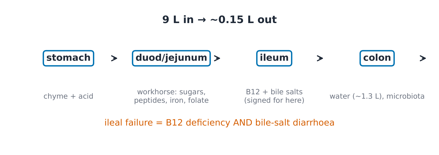
The derivation (why secretion is staged upstream of absorption). Fat digestion needs emulsification (bile) and a near-neutral pH for pancreatic lipase — so the stomach's acid is met by bicarbonate in the duodenum, and the peak of pancreatic secretion arrives exactly where absorption needs it. Staging explains the diseases: pancreatic insufficiency (no enzymes: fats unabsorbed), ileal resection (B12 and bile salts lost: both deficiency AND a bile-salt diarrhoea as they reach the colon).
Worked example 1 — the nine-litre ledger. In: food and drink 2, saliva 1.5, gastric 2.0, bile 0.5, pancreatic 1.5, intestinal 1.5 = 9 L/day ✓; out: ~8.9 L absorbed (small bowel 7.5, colon 1.4), 0.1–0.2 L in stool ✓. Diarrhoea arithmetic: cholera toxin keeps the gut secreting (MED01's welded switch) — litres of stool with an intact mucosa.
Worked example 2 — clinical link: the segment-specific failure. (Fictional) after ileal resection: macrocytic anaemia (B12 needs the ileum-intrinsic factor complex) plus steatorrhoea (bile salts no longer recycled — the pool shrinks below the fat load). One segment's physiology predicts BOTH deficiencies and their timing (bile-salt pool: days to weeks; B12 stores: years).
Common mistakes. Expecting the stomach to be the main absorber (alcohol and aspirin aside, it is not). Forgetting the migrating motor complex — the fasting "housekeeper" cycle that stops with feeding. Treating vomiting as a gastric event (it is medullary, with gastric output as the effector).
Summary. 9 L in / ~0.15 L out; jejunum does the bulk, ileum signs for B12 and bile salts, colon polishes water; enteric plexus under vagal/hormonal modulation; segment failure = segment-specific deficiencies.
Endocrine and reproductive physiology
Why it matters. Hormones are the body's slow control layer — signal by axis, act at a distance, feedback at the top. Every axis obeys one grammar, so learning the grammar once retires a dozen syndromes.
The idea, with a picture. The axis: hypothalamus 下丘脑 (releasing hormone) → pituitary 垂体 (trophic hormone) → target gland 靶腺 (effector hormone) → negative feedback to both higher levels ✓. In reproduction: GnRH → LH/FSH → gonads → sex steroids (plus inhibin selectively on FSH); the menstrual cycle 月经周期 is that axis in 28-day rhythm, ovulation triggered by the oestradiol-driven LH surge — positive feedback flipping the loop's sign once per cycle ✓.

The derivation (why feedback order identifies the lesion). The axis fails at one level; the hormones tell you which: primary (target-gland) failure — low effector, HIGH trophic (feedback released); secondary (pituitary) — low trophic, low effector. One pattern pair, every axis ✓. E.g. (fictional labs) low free T4 with high TSH = the thyroid; low T4 with low TSH = the pituitary/hypothalamus.
Worked example 1 — the thyroid arithmetic. The axis set point: TSH log-linearly tracks free T4 — a small T4 fall doubles TSH ✓, which is why TSH is the screening test: the axis amplifies the primary signal before symptoms exist. Feedback, not sensitivity of assay, is why.
Worked example 2 — clinical link: the cycle's two feedback signs. (Fictional work-up) amenorrhoea with high LH: without ovulation there is little progesterone, and progesterone normally slows the hypothalamic GnRH pulses; faster pulses favour LH over FSH, so LH runs high (the PCOS-pattern logic). One axis diagram plus the sign rule explains the lab pattern and the endometrial risk (unopposed oestrogen).
Common mistakes. Reading single hormone levels without their feedback partner (an unpaired cortisol is nearly meaningless). Forgetting the posterior pituitary stores hypothalamic ADH (it is neural, not a gland fed by trophic hormones). Mixing the two ovarian follicle phases' hormones (oestrogen before, progesterone after the surge).
Summary. Axis: releasing → trophic → effector → two-level feedback; primary failure = high trophic, secondary = low; TSH's log-linear gain makes it the screen; ovulation is one sign flip per cycle — oestradiol's positive feedback driving the LH surge.