This is the ninth course in University Electrical Engineering: electrical
machines and power systems 电机与电力系统. EE07 wrote the field equations;
this course puts them to work — the machines that convert mechanical and
electrical energy, and the networks that move it.
Unit 9.1 builds the magnetic circuit and the transformer 变压器.
Units 9.2–9.4 cover the three machine families: DC, induction, synchronous.
Units 9.5–9.6 widen to the network: per-unit arithmetic and power flow.
Unit 9.7 opens power electronics.
The running story is one small workshop: a 10 kVA transformer feeds a
distribution board; an induction motor drives a compressor; a synchronous
generator stands behind the grid; a buck converter charges the battery backup.
Every machine answer below is checked through a second route — loss
accounting, the equivalent circuit at a limit, or the power balance — and
every per-unit answer by converting back to real units.
Why it matters. The charger that fills your phone in an hour contains a
transformer smaller than a coin, and it works because magnetic flux, like
current, flows in loops through materials that resist it. The same picture,
scaled up a million times, moves power between continents.
The idea, with a picture. A coil of $N$ turns carrying current $I$ is a
pump for flux 磁通: it creates magnetomotive force 磁动势$F = NI$ (ampere-turns).
Flux $\Phi$ (weber) flows around an iron loop of length $l$ and
cross-section $A$, opposed by reluctance 磁阻$R_{m} = \dfrac{l}{\mu A}$, where
$\mu = \mu_{0}\mu_{r}$ is the permeability. This is the magnetic mirror of
Ohm's law:
$$\Phi = \frac{F}{R_{m}}, \qquad \text{just as} \qquad I = \frac{V}{R}.$$
The flux density $B = \Phi/A$ (tesla) is the quantity iron cares about —
power-frequency cores work between about 1.0 and 1.5 T.
One flux loop, two coils: the transformer is just a magnetic circuit shared by two windings
The derivation. Ampère's law around the core gives $H\,l = NI$, with $H$
the field intensity in A/m. With $B = \mu H$ and $\Phi = BA$:
Nothing deeper — the whole unit is bookkeeping on this line, plus one warning:
air has $\mu_{r} = 1$, four thousand times weaker than the core below, so a
tiny air gap 气隙 can dominate the reluctance of the entire loop.
Worked example 1 — a core on its own. A core of mean length 0.5 m,
cross-section 10 cm² $= 10^{-3}$ m², $\mu_{r} = 4000$, wound with 200 turns at
0.5 A. The magnetomotive force is $F = 200 \times 0.5 = 100$ At. The
reluctance is $R_{m} = \dfrac{0.5}{4\pi \times 10^{-7} \times 4000 \times 10^{-3}} = 99\,472$ At/Wb,
so the flux is $\Phi = \dfrac{100}{99\,472} = 1.005$ mWb and the density
$B = \dfrac{1.005 \times 10^{-3}}{10^{-3}} = 1.005$ T. Second route:
$H = NI/l = 200$ A/m, so $B = \mu_{0}\mu_{r}H = 4\pi \times 10^{-7} \times 4000 \times 200 = 1.005$ T ✓ —
a sensible power-frequency density, which is itself the sanity check that the
arithmetic stayed in range.
Now cut a 0.5 mm gap in the same core. The gap adds
$R_{gap} = \dfrac{0.5 \times 10^{-3}}{4\pi \times 10^{-7} \times 10^{-3}} = 397\,887$ At/Wb —
four times the whole core's reluctance. Flux collapses to
$\dfrac{100}{497\,359} = 0.201$ mWb, one fifth, from a gap a hair thick. This
is why transformer cores are stacked and laminated tight, and why gapped cores
must be designed on purpose.
Worked example 2 — the transformer, measured. A transformer links two
windings through one shared flux, so ideally $\dfrac{V_{1}}{V_{2}} = \dfrac{N_{1}}{N_{2}}$
and $\dfrac{I_{1}}{I_{2}} = \dfrac{N_{2}}{N_{1}}$: volts trade against amps,
power stays. Real ones lose a little in the winding resistance (copper
loss 铜损$I^{2}R$) and in the iron (core loss 铁损: hysteresis 磁滞 plus
eddy currents 涡流). The two losses are separated by two tests:
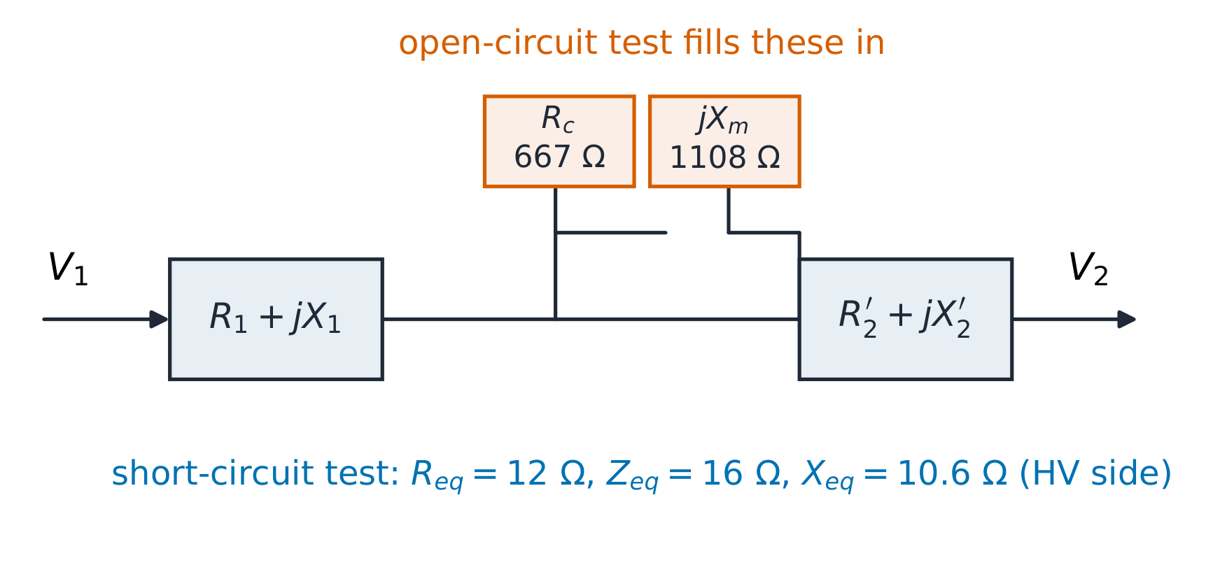
Open-circuit test 空载试验 (LV side, rated voltage): 400 V draws 0.7 A and
240 W. The 240 W is core loss. Its loss current is $I_{c} = 240/400 = 0.6$ A,
so the magnetising branch is $R_{c} = 400/0.6 = 667\ \Omega$ and, from
$I_{m} = \sqrt{0.7^{2} - 0.6^{2}} = 0.361$ A, $X_{m} = 400/0.361 = 1108\ \Omega$
(both referred to the LV side).
Short-circuit test 短路试验 (HV side, reduced voltage, rated current):
80 V draws the rated 5 A ($= 10\,000/2000$) and 300 W. That 300 W is the
full-load copper loss, and the series branch is
$R_{eq} = 300/5^{2} = 12\ \Omega$, $Z_{eq} = 80/5 = 16\ \Omega$,
$X_{eq} = \sqrt{16^{2} - 12^{2}} = 10.6\ \Omega$ (HV side).
Two tests, two branches: the open circuit fills in the shunt pair, the short circuit the series pair
Full-load efficiency at unity power factor:
$\eta = \dfrac{10\,000}{10\,000 + 240 + 300} = 94.9\%$. At 0.8 power factor the
output is 8000 W with the same losses, so $\eta = \dfrac{8000}{8540} = 93.7\%$ —
fixed core loss hurts more as the useful power falls. Efficiency peaks where
the load-dependent copper loss equals the fixed core loss:
$x = \sqrt{240/300} = 0.894$ of full load, a number the workshop should
recognise on its meter.
Common mistakes. Forgetting $\mu_{0}$ inside $\mu$ (a factor of nearly a
million, since $1/\mu_{0} \approx 8 \times 10^{5}$). Referring OC values to the HV side or SC values to the LV side
without squaring the turns ratio. Expecting the ideal-transformer current
ratio to survive heavy loading — the series drop $I \times Z_{eq}$ is exactly
what bends it. And treating an air gap as a small detail: the example above
shows a hair-thick gap is four fifths of the story.
Summary.$F = NI$ drives $\Phi = F/R_{m}$ through reluctance
$l/(\mu A)$; density $B = \Phi/A$ must stay under about 1.5 T. Two tests on a
real transformer separate shunt (core, from the open circuit) from series
(copper, from the short circuit), and efficiency balances output against both.
Why it matters. The motor in a cordless drill, an electric train's axle
motor and the starter in every car with a combustion engine are DC machines:
torque you can command with a current, from two lines of physics.
The idea, with a picture. A conductor of length $l$ in field $B$ carrying
current $I$ feels force $F = BIl$; the same conductor moving at speed $v$
induces EMF $e = Blv$. A DC machine wires many such conductors around a rotor
(the armature 电枢) and commutates them so each sees a fixed field
direction — the commutator 换向器 is a mechanical switch that keeps the
torque unidirectional. Collect the bookkeeping into one constant $k\Phi$ and
the whole machine is two equations:
with $k\Phi$ set by the field flux alone. Multiplying them,
$T\omega = E I_{a}$: the same air-gap power seen from both sides. Mechanical
and electrical language are one language.
The field connection chooses the personality. A shunt motor 并励电机
(field in parallel, constant flux) holds nearly constant speed; a series
motor 串励电机 (field in series, flux $\propto I_{a}$) makes torque
$\propto I_{a}^{2}$ and must never run unloaded.
Shunt: a flat speed for any load. Series: huge torque at low speed, runaway risk at no load
The derivation. From $e = Blv$ with $v = \omega r$ and the geometry
bundled into $k$: $E = k\Phi\omega$. From $F = BIl$ with the lever arms
bundled the same way: $T = k\Phi I_{a}$. In a shunt machine $\Phi$ is fixed by
the supply, so speed follows $\omega = \dfrac{V - I_{a}R_{a}}{k\Phi}$: the
armature resistance drop is the only sag. In a series machine $\Phi \propto I_{a}$
(until iron saturates), so $T \propto I_{a}^{2}$ and
$\omega \propto \dfrac{V - I_{a}R_{a}}{I_{a}}$ — speed rises sharply as load
disappears.
Worked example 1 — the rating point. A shunt motor on 220 V with armature
resistance $R_{a} = 0.2\ \Omega$ draws $I_{a} = 50$ A at 1500 rpm. The EMF is
$E = 220 - 50 \times 0.2 = 210$ V. At 1500 rpm $= 157.1$ rad/s,
$k\Phi = \dfrac{210}{157.1} = 1.337$ V·s, so torque
$T = 1.337 \times 50 = 66.9$ N·m. Check both routes through the air gap:
$T\omega = 66.9 \times 157.1 = 10.5$ kW and $E I_{a} = 210 \times 50 = 10.5$ kW ✓ —
they must agree; they are the same conversion.
Starting the same motor from rest is the trap: at switch-on $E = 0$, so the
inrush would be $I_{a} = \dfrac{220}{0.2} = 1100$ A, twenty times rated. A
starter resistance limiting current to 100 A needs
$R_{start} = \dfrac{220}{100} - 0.2 = 2.0\ \Omega$, cut out in steps as $E$
builds.
Worked example 2 — field weakening. Keep the load torque of 66.9 N·m and
cut the field flux 20%, to $k\Phi = 1.070$. Torque demands
$I_{a} = \dfrac{66.9}{1.070} = 62.5$ A, so the EMF settles at
$E = 220 - 62.5 \times 0.2 = 207.5$ V and the speed at
$\omega = \dfrac{207.5}{1.070} = 193.9$ rad/s $= 1852$ rpm — about 23% faster
for one fifth less flux. Power check: $T\omega = 66.9 \times 193.9 = 12.96$ kW
against $E I_{a} = 207.5 \times 62.5 = 12.97$ kW ✓. Above base speed this is
the standard trick — field weakening 弱磁: trade flux for speed, pay in armature current.
Common mistakes. Feeding rpm into $E = k\Phi\omega$ (it wants rad/s — a
factor of $2\pi$). Expecting a shunt motor to speed up under load (the drop
across $R_{a}$ makes it slow, slightly). Running a series motor unloaded —
with no current there is no flux to limit the speed. And forgetting that at
standstill the only thing limiting current is resistance.
Summary.$E = k\Phi\omega$ and $T = k\Phi I_{a}$, joined by
$T\omega = EI_{a}$. Shunt wiring holds speed; series wiring multiplies torque
at low speed. Start through resistance, weaken field for range.
Why it matters. Around seven of every ten industrial motors are squirrel-cage 鼠笼式 induction machines: no brushes, no commutator, one moving part
— because the rotating field does the switching for free.
The idea, with a picture. Three coils spaced 120° apart, fed by three
currents spaced 120° apart in time, add to a rotating field 旋转磁场 of
constant magnitude that rotates at synchronous speed 同步转速$n_{s} = \dfrac{120f}{p}$ rpm ($f$ in Hz,
$p$ poles). The rotor chases it and never quite catches up; the shortfall is
slip 转差率
$$s = \frac{n_{s} - n}{n_{s}}.$$
Slip is the gear ratio of the machine: the rotor bars see the field slip past
at rate $s$, so the rotor frequency is $sf$ and every rotor quantity follows
from it.
The derivation. In the equivalent circuit, all quantities are referred to
the stator and the rotor branch appears as $R_{2}'/s$ — the slip-scaled
resistance. Split it:
and the second term is not a resistance at all: multiplied by $I^{2}$ it is
exactly the mechanical output power, while $I^{2}R_{2}'$ is the rotor copper
loss. Slip divides the air-gap power
$P_{ag} = T\omega_{s}$ into copper loss $sP_{ag}$ and shaft power
$(1-s)P_{ag}$. With a Thevenin source $V_{th}$, $Z_{th} = R_{th} + jX_{th}$
behind the magnetising branch, torque is
peaking (differentiate, set to zero) where $R_{2}'/s_{max} = \sqrt{R_{th}^{2} + (X_{th} + X_{2}')^{2}}$
— the breakdown torque 最大转矩. Extra rotor resistance moves the peak
towards starting: the wound rotor 绕线转子 machine and the double-cage rotor sell exactly this.
Same peak torque, different address: rotor resistance chooses where the curve peaks
Worked example 1 — reading the nameplate. A 4-pole, 50 Hz motor: $n_{s} = \dfrac{120 \times 50}{4} = 1500$ rpm.
Running at 1440 rpm: $s = \dfrac{60}{1500} = 0.04$. The rotor frequency is
$sf = 2$ Hz — why rotor iron needs only light laminations — and the slip term
$R_{2}'/s$ is $25 \times R_{2}'$: at small slip the rotor behaves almost
purely resistively, which is why the machine runs efficiently near
synchronism.
Worked example 2 — the whole torque chain. The same motor, 400 V line
(231 V per phase), $R_{1} = 0.5$, $X_{1} = 1.2$, $R_{2}' = 0.4$,
$X_{2}' = 1.2\ \Omega$, magnetising branch large (taken out of the way:
$V_{th} = 231$ V, $Z_{th} = R_{1} + jX_{1}$). Synchronous speed
$\omega_{s} = 157.1$ rad/s. At $s = 0.04$, $R_{2}'/s = 10\ \Omega$:
Follow the power: $P_{ag} = T\omega_{s} = 13.8$ kW, rotor copper loss
$sP_{ag} = 552$ W, shaft power $T\omega_{s}(1-s) = 13.2$ kW ✓ — one chain of
multiplications, three balances closed. The peak:
$s_{max} = \dfrac{0.4}{\sqrt{0.5^{2} + 2.4^{2}}} = 0.163$, and the breakdown
torque there is 172 N·m — twice the running point, the margin the compressor
start needs. Locked rotor ($s = 1$): $T_{start} = 62$ N·m. Double the rotor
resistance and $T_{start}$ rises to 109 N·m while the running point (same
slip) loses efficiency — the wound-rotor trade in one number.
Common mistakes. Mixing rpm and rad/s inside the torque formula
($\omega_{s}$ is mechanical, rad/s). Assuming torque rises with slip — it
peaks at $s_{max}$ and falls both sides. Charging the whole air-gap power to
copper loss: copper gets only the fraction $s$. And expecting the rotor
frequency to be 50 Hz — it is $sf$, 2 Hz here.
Summary.$n_{s} = 120f/p$, slip $s = (n_{s}-n)/n_{s}$, rotor frequency
$sf$, rotor branch $R_{2}'/s$ whose second half is the shaft. Torque peaks
where $R_{2}'/s$ matches the magnitude of $R_{th} + j(X_{th} + X_{2}')$; rotor resistance buys
starting torque at running cost.
探索
磁场旋转,转子追赶
Move the slip and watch the stator field, the rotor and their relative speed; read the rotor frequency off the gap between them.
Why it matters. Virtually every watt from a power station flows out of a synchronous machine 同步电机: a magnet spun by a turbine, locked to the grid's
rotating field, delivering power through an angle.
The idea, with a picture. The rotor — an electromagnet or permanent
magnet — locks to the rotating field, so speed is exactly $n_{s} = 120f/p$,
no slip. The induced EMF has the transformer form
$E = 4.44\, f N \Phi k_{w}$ (the winding factor $k_{w}$ tidies the coil
geometry). What the machine exchanges with the grid is set by the power
angle 功率角$\delta$: the angle by which the rotor's EMF leads the bus
voltage. The connection behaves like a torsion spring — deflect it, feel
torque:
$$P = \frac{3 V E}{X_{s}} \sin\delta .$$
A sine-shaped spring: power grows with angle to 90 degrees, then lets go — that is loss of synchronism
The derivation. Per phase, the bus is $V\angle 0$, the internal EMF
$E\angle\delta$, between them only the synchronous reactance $X_{s}$:
The $Q$ line carries the second lesson: raising the field (excitation励磁) raises $E$ and pushes $Q$ positive — the machine exports reactive power
like a capacitor; lowering it imports. Grid operators schedule this daily.
Worked example 1 — the rating and its margin. A generator on an
infinite bus 无穷大母线 at 11 kV line, $X_{s} = 5\ \Omega$ per phase,
EMF 12 kV line. Per phase $V = 6351$ V, $E = 6928$ V, so
At $\delta = 30°$: $P = 13.2$ MW. The static margin 静态裕度 is
$\dfrac{26.4 - 13.2}{13.2} = 100\%$ — the machine could double its load before
the spring lets go. Operators keep real machines nearer 30° for exactly this
cushion.
Worked example 2 — real and reactive together. Same machine, schedule
10 MW: $\sin\delta = \dfrac{10}{26.4} = 0.379$, $\delta = 22.3°$. Then
Over-excited, it quietly supports the bus voltage while delivering the
megawatts. Under-excite to $E = 10$ kV line (5774 V per phase) and hold
10 MW: $\sin\delta = \dfrac{10 \times 5 \times 10^{6}}{3 \times 6351 \times 5774} = 0.455$,
$\delta = 27.0°$, and
$Q = \dfrac{3 \times 6351 \times (5774 \times 0.890 - 6351)}{5} = -4.6$ MVAr:
the same megawatts, but the machine now absorbs reactive power. One dial
(excitation) moves Q far more than P.
Common mistakes. Using line voltages per phase (divide by $\sqrt{3}$
first). Believing more excitation gives more real power — the turbine sets
$P$; excitation sets $Q$. Pushing $\delta$ past 90°, where
$\dfrac{dP}{d\delta}$ goes negative and the machine slips a pole. And
forgetting that $\delta$ here is electrical: with $p$ poles the mechanical
angle is $2\delta/p$.
Summary. Speed locked to the grid, power $P = \dfrac{3VE}{X_{s}}\sin\delta$,
reactive $Q = \dfrac{3V(E\cos\delta - V)}{X_{s}}$. Turbine owns the angle,
field owns the VARs.
Why it matters. A grid calculation mixing ohms at 11 kV with ohms at
132 kV drowns in turns ratios. Power engineers long ago switched to a language
where every voltage is near 1.0 and every impedance is a percentage: the
per-unit 标幺值 system.
The idea, with a picture. Choose a base value 基准值 pair: base power $S_{base}$ and base
voltage $V_{base}$ at each level; everything else follows:
Impedances move between voltage levels by the turns ratio squared — per-unit
absorbs that automatically, because each level has its own $Z_{base}$. A
transformer's nameplate "10%" means: at its own rated current, 10% of rated
voltage drops inside it — which is exactly $Z_{pu} = 0.10$.
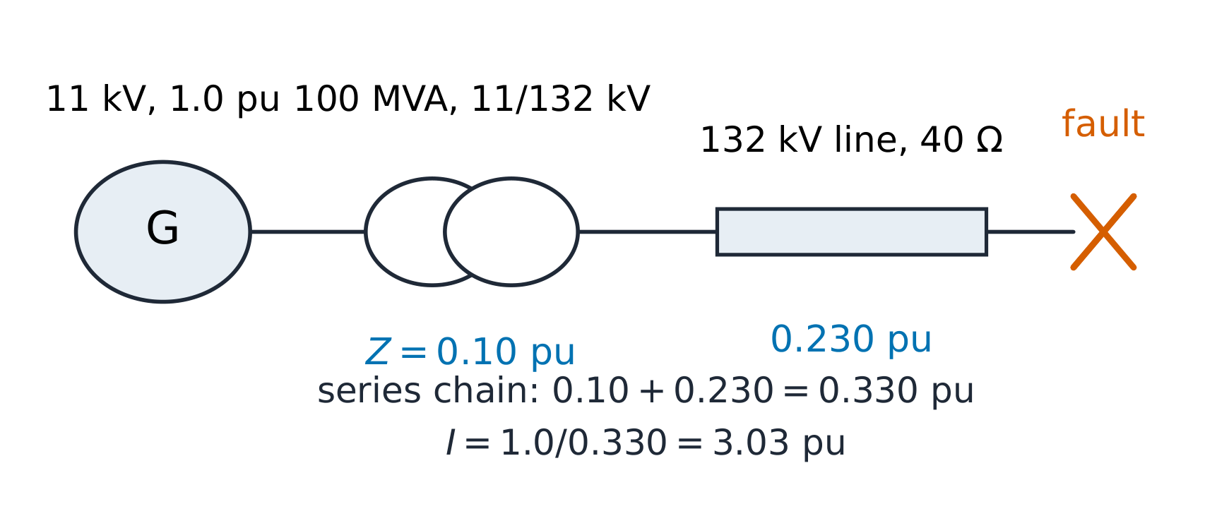
One line, one chain of per-unit impedances: the fault sees them all in series
The derivation. Base changes are pure bookkeeping. An impedance given as
$Z_{old}$ pu on $S_{old}$, $V_{old}$ becomes, on new bases,
and if the voltage bases already match the transformer ratio (as they do in a
consistent study), only the $S$ ratio survives.
Worked example 1 — a fault at the end of the line. A 100 MVA, 11/132 kV
transformer with $Z = 10\%$ on its own base feeds a 132 kV line of 40 Ω; a
three-phase fault closes at the line's far end with the generator held at
1.0 pu. Line base: $Z_{base} = \dfrac{132^{2}}{100} = 174.2\ \Omega$, so the
line is $\dfrac{40}{174.2} = 0.230$ pu; the transformer is already 0.10 pu on
100 MVA. Total $0.330$ pu, so the fault current 短路电流 is
$\dfrac{1.0}{0.330} = 3.03$ pu. Back to real units — the check that proves
the method: base current at 132 kV is
$I_{base} = \dfrac{100 \times 10^{6}}{\sqrt{3} \times 132\,000} = 437$ A, so
$I_{fault} = 3.03 \times 437 = 1327$ A. The same 3.03 pu read on the 11 kV
side with that level's base current
$\dfrac{100 \times 10^{6}}{\sqrt{3} \times 11\,000} = 5249$ A gives
$3.03 \times 5249 = 15\,926$ A — one dimensionless number serves both voltage levels ✓.
Worked example 2 — changing bases. The study grows: add a 60 MVA,
66/11 kV transformer rated 8% and a generator with $X_{d} = 0.25$ pu on
80 MVA, 11 kV. On the study's 100 MVA base the transformer becomes
$0.08 \times \dfrac{100}{60} = 0.133$ pu and the generator
$0.25 \times \dfrac{100}{80} = 0.313$ pu (voltage bases already agree). In
series between the generator's EMF and a fault on the transformer's 66 kV
terminals: $0.313 + 0.133 = 0.446$ pu, so the fault current is
$\dfrac{1.0}{0.446} = 2.24$ pu. On the 66 kV side the base current is
$\dfrac{100 \times 10^{6}}{\sqrt{3} \times 66\,000} = 875$ A, so
$2.24 \times 875 = 1962$ A flows into the fault, while the generator carries
$2.24 \times 5249 = 11\,780$ A on its 11 kV side — the same pu, two real currents.
Two multiplications replaced a page of ratio chasing.
Common mistakes. Using line-to-line volts in a per-phase base (or
vice versa) — pick the convention $Z_{base} = V_{LL}^{2}/S_{3\phi}$ and stay
with it. Forgetting the square on the voltage-base ratio when changing bases.
And treating "%Z" as a loss figure — it is a voltage-drop figure at rated
current, which is why a 10% transformer can still be 99% efficient at full
load.
Summary. Choose $S_{base}$ once and $V_{base}$ per level; convert
everything to pu; series, parallel and fault arithmetic go dimensionless;
convert back with each level's own base current to prove the answer.
Why it matters. "Will the voltage at the end of the feeder stay above
0.95?" is the question every grid planner answers thousands of times a day
with a power flow 潮流计算 — and the two-bus version fits on one page.
The idea, with a picture. Bus 1 is the slack bus 平衡节点: held at
$1.0\angle 0°$ pu, absorbing whatever the losses turn out to be. A line
$Z = R + jX$ feeds a load drawing $S = P + jQ$ at bus 2. The load fixes
current through its own voltage, and the voltage fixes current through the
line — a loop. So guess $V_{2}$, run the loop once, and repeat:
$$V_{2}^{(k+1)} = V_{1} - Z \cdot \mathrm{conj}\!\left(\frac{S}{V_{2}^{(k)}}\right),$$
the fixed-point (Gauss–Seidel) iteration. The conjugate is not decoration:
with $S = V I^{*}$, the current is $I = \mathrm{conj}(S/V)$, and skipping it
sends the iteration to nonsense.
Guess, correct, repeat: both cases settle within a few iterations — and compensation settles higher
The derivation. From $V_{2} = V_{1} - ZI$ and $I^{*} = S/V_{2}$, each
pass computes the current the present $V_{2}$ implies and the voltage that
current produces. Linearise once around $V \approx 1$ and the famous
approximation falls out:
$$\Delta V \approx \frac{P R + Q X}{|V_{2}|},$$
whose second term explains the unit's headline: it is the reactive flow
through reactance that eats voltage, which is why capacitors — reactive
compensation 无功补偿 — are a voltage tool.
Worked example 1 — the base case.$Z = 0.02 + j0.10$ pu, load
$0.8 + j0.4$ pu, $V_{1} = 1.0\angle 0°$. Starting from $V_{2} = 1.0$ the
iteration converges to $V_{2} = 0.937\angle -4.4°$ pu, with line current
$I = 0.954\angle -31°$ pu. Checks: the approximation gives
$\Delta V \approx \dfrac{0.8 \times 0.02 + 0.4 \times 0.10}{0.937} = 0.060$ pu
against the exact $1 - 0.937 = 0.063$ ✓ honest at this loading; of the drop,
$QX = 0.040$ dwarfs $PR = 0.016$ — reactive dominates. The sending-end
balance: $P_{s} = 0.8 + |I|^{2}R = 0.8 + 0.954^{2} \times 0.02 = 0.818$ pu ✓
and $Q_{s} = 0.4 + 0.954^{2} \times 0.10 = 0.491$ pu: the line itself eats
0.091 of reactive.
Worked example 2 — compensation. Install capacitors at bus 2 cutting the
net load to $0.8 + j0.1$ pu and iterate again: $V_{2}$ settles at
$0.970\angle -4.6°$ pu. The drop falls from 0.063 to 0.030 pu — the $QX$ term
dropped from 0.040 to 0.010 and the voltage followed — while the angle stays
near 4.5°, because the angle is carried by $P$, which did not change. In
per-unit the design sentence is one line: 0.3 pu of capacitors at the load
lifts $V_{2}$ as far as halving the line impedance would (0.970 pu either
way), and capacitors cost far less than a second line.
Common mistakes. Dropping the conjugate (the iteration then diverges or
converges to a wrong operating point quietly). Letting the slack bus fix
more than it should — it sets the angle reference and swallows losses;
loads elsewhere must still balance in the converged answer. And trusting
$\Delta V \approx (PR + QX)/V$ when the angle across the line grows: the
approximation quietly ignores the quadrature component $\dfrac{PX - QR}{V}$,
fine here at 4.4°, misleading past about 15°.
Summary. Slack at one end, load at the other, iterate
$V_{2} = V_{1} - Z\,\mathrm{conj}(S/V_{2})$; verify with the $PR + QX$
approximation and close the power balance. Reactive flow is the voltage
problem; compensation is the cheap half of the fix.
Why it matters. The same charger opens with a switch that flips a hundred
thousand times a second. Switching converters are why a 30-watt adapter is
now smaller than its own plug — and why this unit ends the course: machines
meet electronics at the drive.
The idea, with a picture. A buck 降压 converter is a switch, a diode,
an inductor and a capacitor. While the switch is ON the input feeds the
inductor; while it is OFF the inductor keeps current flowing through the
diode. The inductor and capacitor do the averaging; the switch only chooses
the ratio of on-time to period, the duty cycle 占空比$D$. Volt-second
balance 伏秒平衡 on the inductor — the average of $v_{L}$ over a period must be zero
in steady state — gives, in one line:
$$(V_{in} - V_{out})\,D T = V_{out}\,(1-D)\,T \quad\Longrightarrow\quad V_{out} = D\,V_{in},$$
and the boost 升压 dual gives $V_{out} = \dfrac{V_{in}}{1-D}$. Continuous
conduction 连续导通 (CCM) means the inductor current never reaches zero —
the small-ripple world all these formulas live in.
Inductor current ramps up while the switch is on and down while it is off
The derivation. In continuous conduction, the buck ON phase the inductor sees $V_{in} - V_{out}$
for $DT$ seconds; in the OFF phase $-V_{out}$ for $(1-D)T$. Setting the
volt-second sum to zero yields $V_{out} = D V_{in}$ — independent of L, C and
load in CCM, which is the converter's charm. The triangular current swing
follows from $v = L\,di/dt$ on either phase:
Worked example 1 — a 12 V to 5 V buck. Twelve volts in, 5 V at 2 A out,
switching at 100 kHz with $L = 100\ \mu$H. Duty $D = \dfrac{5}{12} = 0.417$.
Ripple current $\Delta I_{L} = \dfrac{5 \times 0.583}{100\mu \times 100k} = 0.29$ A —
15% of the load, a standard design point. CCM holds because
$\Delta I_{L}/2 = 0.15$ A is far below 2 A. With $C = 220\ \mu$F the output
ripple is $\Delta V_{out} = \dfrac{0.29}{8 \times 220\mu \times 100k} = 1.7$ mV:
the converter's output is cleaner than the supply it runs from.
Worked example 2 — a 12 V to 24 V boost. The boost runs the same parts
re-arranged: switch across the inductor, diode to the output. For 24 V at
1.5 A from 12 V, $D = 1 - \dfrac{12}{24} = 0.5$. Power conserved (ideal):
$P_{in} = 36$ W, so the input current is 3 A — not 1.5 A; current trades
against voltage, power does not. Ripple
$\Delta I_{L} = \dfrac{V_{in} D}{L f} = \dfrac{12 \times 0.5}{100\mu \times 100k} = 0.6$ A,
CCM comfortable against 3 A. The output capacitor sees the diode's chopped
current — pulses only during $(1-D)$ of each period — so boost converters
need bigger, lower-ESR output capacitors than bucks of the same power:
the ripple RMS, not the average, sizes the part.
Common mistakes. Light load in a "CCM" design: below the boundary
current $\Delta I_{L}/2$ the converter drops into discontinuous conduction
and $V_{out}$ rises above $D V_{in}$. Ignoring the diode drop in low-voltage
outputs — 0.4 V in a 5 V rail is 8%, which is why synchronous
rectification 同步整流 (a MOSFET for the diode) is routine below about
12 V. And equating input and output current because the topology looks
symmetric — only power is conserved.
Summary. Volt-second balance: $V_{out} = D V_{in}$ (buck) or
$V_{out} = V_{in}/(1-D)$ (boost) in CCM; ripples
$\Delta I_{L} = \dfrac{V_{out}(1-D)}{Lf}$ and $\Delta V_{out} = \dfrac{\Delta I_{L}}{8Cf}$.
The switch sets the ratio; the passives set the quality; the losses live in
the switch and the diode.