This is the fourth course in University Electrical Engineering: AC circuit
analysis 交流电路分析 — circuits driven by sinusoids, which is how almost all
electrical energy is generated and moved. Wave 1 solved DC; the tools of EE02
(complex numbers, differential equations, Laplace) now pay for themselves.
Unit 4.1 makes sinusoids arithmetic: the phasor and the impedance.
Units 4.2–4.4 apply it: AC power, three-phase, second-order response and
resonance.
Units 4.5–4.7 widen the view: filters and Bode plots, s-domain circuit
analysis, and two-port networks.
Each unit opens with a story, shows a picture before the formal idea, defines
terms precisely, works two escalating examples whose numbers are
machine-verified, names the classic mistakes, and closes with a three-line
summary. The checking habit: every phasor answer verifies in a second
representation — polar against rectangular, or the time domain against the
complex arithmetic. Complex arithmetic is only bookkeeping; the checks keep it
honest.
The mains voltage crosses zero a hundred times a second, yet a resistor there
dissipates steady power — because amplitude and phase settle into a repeating
pattern. A sinusoid $v(t) = V_{m}\cos(\omega t + \varphi)$ becomes a phasor相量$V = V_{m}\angle\varphi$ — the amplitude and phase, with the frequency
understood. Differentiating multiplies by $j\omega$; so at a single frequency
every element gets an impedance 阻抗:
$$Z_R = R \qquad Z_L = j\omega L \qquad Z_C = \frac{1}{j\omega C}$$
All the DC methods — dividers, node/mesh, Thévenin — carry over unchanged with
complex numbers. The inductor's impedance grows with frequency (+90°); the
capacitor's shrinks (−90°); the resistor is flat (0°).
The rotating picture behind the frozen phasors: ratio questions cancel the rotation, so the snapshot is enough
Worked example 1 (both representations agree).$R = 30\ \Omega$ in series
with $L$ such that $\omega L = 40\ \Omega$, driven by $V = 100\angle 0^{\circ}$
V at that frequency. $Z = 30 + j40 = 50\angle 53.13^{\circ}\ \Omega$;
$I = V/Z = (100/50)\angle(0 - 53.13^{\circ}) = 2\angle -53.13^{\circ}$ A. Check
in rectangular: $I = 100(30 - j40)/2500 = 1.2 - j1.6$ A; $|I| =
\sqrt{1.44 + 2.56} = 2$ ✓ and $\text{atan2}(-1.6, 1.2) = -53.13^{\circ}$ ✓.
The time-domain meaning: $i(t) = 2\cos(\omega t - 53.13^{\circ})$ A — the
current lags because the inductor opposes change.
Worked example 2 (parallel combination, escalated). The same $R = 30\ \Omega$
now in parallel with the $\omega L = 40\ \Omega$ inductor:
$Z = \frac{30 \times j40}{30 + j40} = \frac{30 \times j40 \times
(30 - j40)}{2500} = \frac{48\,000 + j36\,000}{2500} = 19.2 + j14.4 =
24\angle 36.87^{\circ}\ \Omega$ (verified:
$|Z| = \sqrt{19.2^{2} + 14.4^{2}} = 24$ ✓, and $\cos 36.87^\circ = 0.8$ ✓).
Note the parallel impedance is smaller than either branch magnitude
(24 < 30 < 40) and its angle (36.87°) lies below the inductor's 90°,
pulled toward the resistor — every parallel pair trades magnitude and angle
in this direction.
Common mistakes. Adding magnitudes of parallel impedances (only complex
addition is legal). Mixing degree-mode calculator settings into radian
formulas. Forgetting that the phasor carries amplitude (or RMS — pick one
convention per problem) consistently for V and I.
Summary: one frequency → phasors; $Z_R$ flat, $Z_L$ up 90°, $Z_C$ down 90°;
every DC method carries over; verify each answer in the other representation.
A 1 kW heater and a 1 kVA capacitor both draw "1 k-something" from the line,
but only the heater's share bills as energy. With phasor $V$ and current $I$,
complex power 复功率$S = V\cdot I^{*}$:
with $\theta$ the angle between V and I. The power factor 功率因数$\cos\theta$ is the fraction of apparent power $|S| = VI$ that does real work.
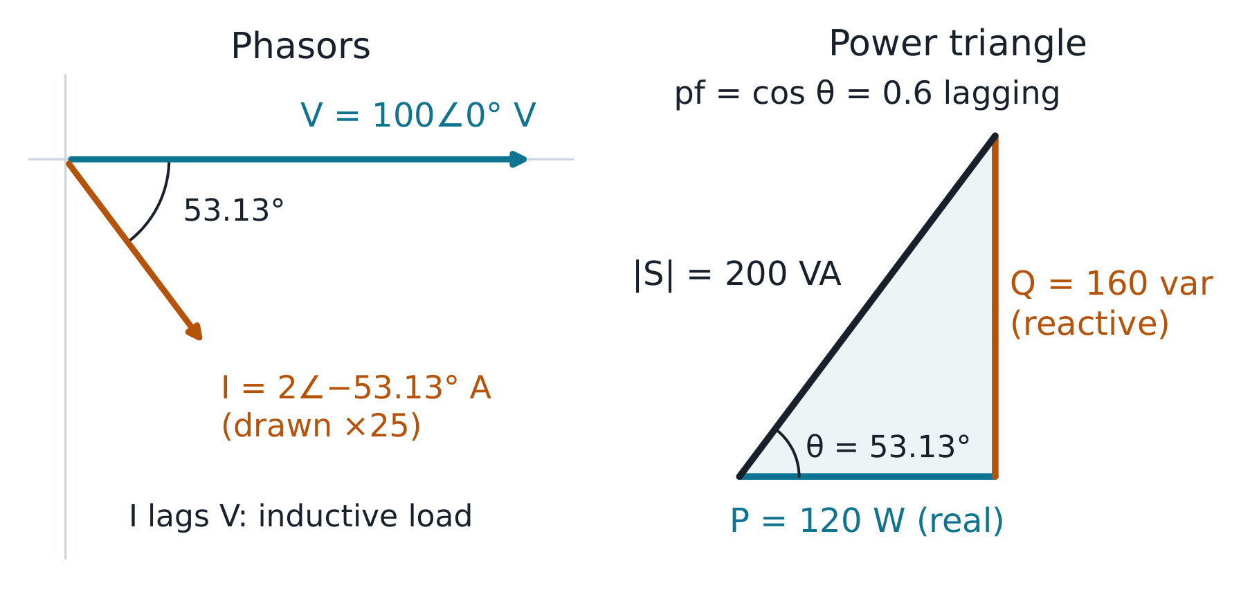
The RL load: current lags by 53.13°, so P = 120 W, Q = 160 var and pf = 0.6 lagging
Worked example 1 (the RL load, checked two ways). The load above:
$P = 100 \times 2 \times \cos 53.13^{\circ} = 120$ W, $Q = 100 \times 2 \times
\sin 53.13^{\circ} = 160$ var, $|S| = 200$ VA, pf = 0.6 lagging. Check:
$P = |I|^{2}R = 4 \times 30 = 120$ ✓ and $Q = |I|^{2}X = 4 \times 40 = 160$ ✓
— the loss-formula check. Power-factor correction 功率因数校正 adds parallel
capacitance to supply the reactive power locally: to correct 160 var at 100 V
(50 Hz) needs $C = Q/(\omega V^{2}) = 160/(2\pi \cdot 50 \cdot 10^{4}) =
50.9\ \mu F$.
Worked example 2 (a three-phase motor, escalated). A balanced star-connected
motor on a 415 V (line), 50 Hz supply has phase impedance $10 + j10\ \Omega$
per phase. Phase voltage $= 415/\sqrt{3} = 239.6$ V; phase current
$= 239.6/\sqrt{10^{2} + 10^{2}} = 239.6/14.14 = 16.94$ A (equal to line
current in star); phase angle 45° lagging. Total power
$P = 3 \times 239.6 \times 16.94 \times \cos 45^{\circ} = 8611$ W — and the
line formula $\sqrt{3} \times 415 \times 16.94 \times 0.7071 = 8611$ W ✓ the
two routes agree. The per-phase route also gives the missing pieces: $Q = 3
\times 239.6 \times 16.94 \times \sin 45^{\circ} = 8611$ var, pf 0.707
lagging, and (for a delta-connected motor of the same impedance) the phase
current would be $415/14.14 = 29.3$ A with line current $\sqrt{3} \times
29.3 = 50.8$ A — the star/delta factor is exactly the $\sqrt{3}$ bookkeeping.
Common mistakes. Using line voltage in the per-phase formula (divide by
$\sqrt{3}$ first). Forgetting the motor's pf applies to both formulas.
Correcting power factor at the wrong voltage — the capacitor sees the voltage
at its own connection point.
Summary: $S = VI^{*}$ splits into P (billed) and Q (borrowed); loss formulas
$|I|^{2}R$, $|I|^{2}X$ are the check; capacitive correction supplies Q
locally; three-phase per-phase analysis with $V_{line} = \sqrt{3}V_{phase}$
(star) is the workhorse.
Close a switch on a charged capacitor in series with an inductor and the
current cannot jump — nor can it arrive instantly — so the response bends
through at least one derivative more than RC ever needed. A series RLC has the
differential equation $L\,d^{2}i/dt^{2} + R\,di/dt + i/C = 0$, with natural
frequency 固有频率$\omega_{0} = 1/\sqrt{LC}$ and damping 阻尼$\alpha = R/(2L)$. Three regimes:
Overdamped 过阻尼 ($\alpha > \omega_{0}$): two real decays, no oscillation.
One circuit, three resistors: the same ω₀ = 10 rad/s with α = 20, 10 and 5
Worked example 1 (regime arithmetic).$R = 4\ \Omega$, $L = 0.2$ H,
$C = 0.05$ F: $\omega_{0} = 1/\sqrt{0.2 \times 0.05} = 10$ rad/s;
$\alpha = 4/(2 \times 0.2) = 10$ — critically damped ($\alpha = \omega_{0}$).
Change $R$ to 2 Ω: $\alpha = 5 < 10$, underdamped with $\omega_{d} =
\sqrt{100 - 25} = 8.66$ rad/s. The regime test is one comparison; the
Q factor 品质因数$Q = \omega_{0}/(2\alpha)$ is 0.5 at critical damping and
1 at $R = 2\ \Omega$ — lightly damped (high Q) rings longer.
Worked example 2 (the overdamped exponents, machine-verified, escalated).
With $R = 8\ \Omega$ (same $L$, $C$): $\alpha = 20 > 10$ — overdamped, and the
two decay exponents are $s = -\alpha \pm \sqrt{\alpha^{2} - \omega_{0}^{2}} =
-20 \pm \sqrt{300}$, i.e. $-2.68$ and $-37.32$ s⁻¹ (machine-verified). The
capacitor voltage released from 1 V is $v_{C}(t) = A e^{-2.68t} + B
e^{-37.32t}$ with $A + B = 1$ and $dv_{C}/dt(0) = 0$ (no instantaneous
current), giving $A = 37.32/(37.32 - 2.68) = 1.077$, $B = -0.077$: a fast
initial drop onto the slow decay. The reading: the fast root only sets the
first moments; the slow root ($-2.68$, the one nearer the origin) owns the
tail — exactly the dominant-pole rule EE02 met in Laplace.
Common mistakes. Comparing $R$ with $2\sqrt{L/C}$ instead of $\alpha$ with
$\omega_{0}$ — the same test, but write it as stated. Using $\omega_{0}$ where
$\omega_{d}$ belongs (the ringing you see is the damped frequency).
Forgetting the second initial condition: two energy stores give two constants.
Summary: $\omega_{0} = 1/\sqrt{LC}$, $\alpha = R/2L$, three regimes by one
comparison; $\omega_{d}$ is the visible ringing; the slow root owns the tail;
two stores → two constants → two endpoint checks.
A radio's tuning circuit picks one station out of a crowded band by making one
frequency special: at resonance 谐振 the imaginary parts cancel,
$\omega_{0}L = 1/(\omega_{0}C)$, i.e. $\omega_{0} = 1/\sqrt{LC}$. There
$Z = R$ (purely resistive, minimum), current is maximum, and the
bandwidth 带宽$BW = R/L = \omega_{0}/Q$. The halves of the impedance cancel
even though each alone can be large — $V_{L}$ and $V_{C}$ can each exceed the
source voltage by the factor Q.
|Z| dips to R at ω₀; the half-power points sit where |Z| = √2·R
Worked example 1 (voltage magnification, checked).$R = 5\ \Omega$,
$L = 0.1$ H, $C = 10\ \mu F$: $\omega_{0} = 1/\sqrt{0.1 \times 10^{-5}} =
1000$ rad/s; $Q = \omega_{0}L/R = 1000 \times 0.1/5 = 20$. At a source of
10 V, the current at resonance is $10/5 = 2$ A, and $V_{L} = \omega_{0}LI =
200$ V — twenty times the source. Check: $V_{C} = I/(\omega_{0}C) =
2/0.01 = 200$ V ✓; both are 200 V, 180° apart, their sum zero.
Worked example 2 (the half-power band, escalated). The same circuit's
bandwidth: $BW = \omega_{0}/Q = 1000/20 = 50$ rad/s, and the half-power
frequencies compute to $\omega_{1} = 975.3$, $\omega_{2} = 1025.3$ rad/s —
their difference is 50.0 ✓ (machine-verified). They sit almost evenly either
side of 1000; exactly, $\omega_{1}\omega_{2} = \omega_{0}^{2}$ (symmetric on a
logarithmic axis).
At the band edges $|Z| = \sqrt{2}R = 7.07\ \Omega$, the current is
$1/\sqrt{2}$ of maximum, and each reactive element holds
$Q/\sqrt{2} \approx 14$ times the source voltage — still amplification, just
past its peak. This is the selectivity a tuner sells: at 900 rad/s (a
neighbouring station two bandwidths away) the current is down to
$10/\sqrt{R^{2} + (\omega L - 1/\omega C)^{2}} = 10/|5 + j(90 - 111.1)| =
10/21.7 = 0.46$ A — under a quarter of the resonant 2 A.
Common mistakes. Reporting $Q$-amplification without checking the other
element (both must match). Using $f_{0}$ where $\omega_{0}$ belongs (factor
$2\pi$). Believing resonance maximises power at any source impedance — it
minimises |Z|, which maximises current only for a stiff source.
Summary: $\omega_{0} = 1/\sqrt{LC}$, |Z| = R there, BW = ω₀/Q between the
half-power points; each reactive voltage is Q·source; check the amplification
on both elements.
A bass boost is a filter: one band up, the rest untouched. A filter 滤波器
passes a band and attenuates the rest; its transfer function $H(j\omega)$ has
magnitude and phase. The Bode plot 波特图 plots $20\log_{10}|H|$ in dB
against log frequency: each pole contributes −20 dB/decade above its corner
frequency 转折频率$\omega_{c} = 1/(RC)$; each zero +20 dB/decade.
RC low-pass with its corner at 6250 rad/s: exact curves against the straight-line asymptotes
Worked example 1 (the low-pass, endpoints checked). A low-pass RC with
$R = 1.6$ kΩ, $C = 0.1\ \mu F$: $\omega_{c} = 1/(1600 \times 10^{-7}) =
6250$ rad/s (995 Hz). At $\omega_{c}$ the gain is $1/\sqrt{2} = -3$ dB and the
phase −45°; at $10\omega_{c}$ the straight-line approximation reads −20 dB
(exact −20.04). Check the endpoints: at low frequency $H = 1$ (0 dB), at
$100\omega_{c}$ ≈ −40 dB — each decade past the corner loses 20 dB, which is
the decibel 分贝 arithmetic $20\log_{10}10 = 20$.
Worked example 2 (the high-pass mirror, machine-verified, escalated).
Swapping output to the resistor makes a high-pass with the same
$\omega_{c} = 6250$ rad/s: $H(j\omega) = (j\omega/\omega_{c})/(1 +
j\omega/\omega_{c})$. At $0.1\omega_{c}$: $-20.04$ dB at $+84.3^{\circ}$; at
$\omega_{c}$: $-3.01$ dB at $+45^{\circ}$; at $10\omega_{c}$: $-0.04$ dB at
$+5.7^{\circ}$ (all machine-verified) — the exact mirror of the low-pass, with
phase leading and the stop-band below instead of above. The design reading:
a steeper 40 dB/decade roll-off needs two cascaded sections, and (with the
loading between them accounted for) the cascade multiplies gains, so the dB
add — the same chaining logic as the ABCD matrices of unit 4.7.
Common mistakes. Reading −3 dB as "half power lost in the filter" at the
corner (it is half power delivered to the load versus mid-band). Mixing
$\omega$ and $f$ on the same axis. Forgetting phase: a filter that is flat in
magnitude can still wreck a pulse by its phase slope.
Summary: poles −20 dB/decade above their corner, zeros +20; −3 dB and ±45° at
the corner; the asymptotes are the design tool, the exact curve the check.
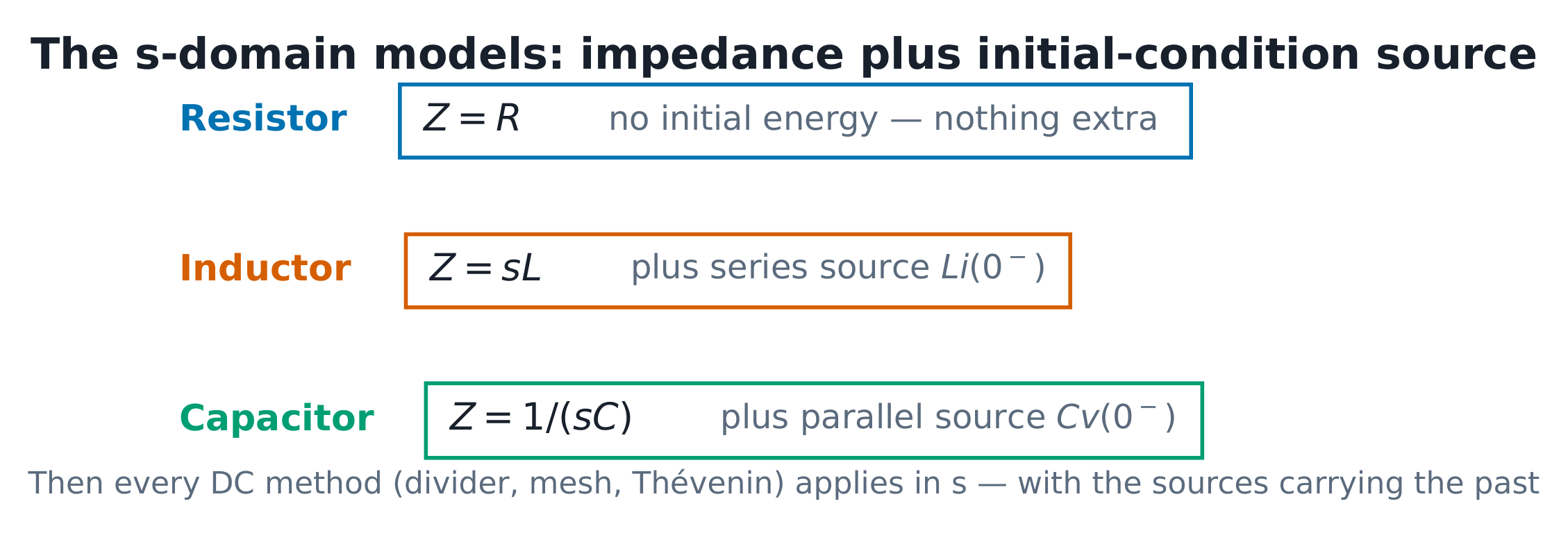
EE02's Laplace machinery becomes a circuit method: each element gets an
s-domain model with initial conditions as sources —
Resistor: $Z = R$.
Inductor: $Z = sL$plus a series voltage $Li(0^{-})$ (or parallel
current source $i(0^{-})/s$).
Capacitor: $Z = 1/(sC)$plus a parallel current source $Cv(0^{-})$ (or
series voltage $v(0^{-})/s$).
Then every DC method applies in $s$. The response's poles carry the
transient; the input's poles carry the steady state.
The s-domain models: impedance plus initial-condition source — one picture for every transient problem
Worked example 1 (the wave-1 RC, by algebra). The wave-1 RC step with
initial voltage: $R = 10$ kΩ, $C = 100\ \mu F$ ($\tau = 1$ s), source 9 V,
$v_{C}(0) = 1$ V. s-domain KVL: $9/s = IR + v_{C}(0)/s + I/(sC)$ →
$I = 8/(R(s + 1/(RC))) = 8/(10^{4}(s+1))$;
$V_{C} = v_{C}(0)/s + I/(sC) = 1/s + 8/(s(s+1)) = 9/s - 8/(s+1)$, so
$v_{C}(t) = 9 - 8e^{-t}$ V — exactly the wave-1 answer, now derived by
algebra. The check: $v_{C}(0) = 9 - 8 = 1$ ✓, $v_{C}(\infty) = 9$ ✓.
Worked example 2 (a source-free RLC, poles matched, escalated). The
series RLC of unit 4.3 with $R = 2\ \Omega$, $L = 0.2$ H, $C = 0.05$ F,
released with $i(0) = 1$ A, $v_{C}(0) = 0$. s-domain mesh (impedances plus the
inductor's $Li(0)$ source): $(0.2s + 2 + 20/s)I = 0.2$, so
$I(s) = s/(s^{2} + 10s + 100)$ and the poles are $-5 \pm j8.66$ — exactly the
$\alpha = 5$, $\omega_{d} = 8.66$ the time-domain regime arithmetic gave ✓.
The two routes are the same physics in two notations; the s-domain route
delivers the exponents without memorising a form, and partial fractions (as in
EE02) finish the waveform.
Common mistakes. Dropping the initial-condition sources — the answer then
claims the circuit starts at rest. Cancelling $s$ blindly (a factor of $s$ in
numerator and denominator can hide an impulse). Forgetting the final-value
theorem's condition (pole strictly in the left half-plane).
Summary: impedances become $R$, $sL$, $1/sC$ plus initial-condition sources;
DC methods in $s$; the poles are$\alpha$ and $\omega_{d}$; endpoint checks
still free.
4.7
双口网络
English
An amplifier module, a matching network, a length of cable — each is a box
with two wire pairs, and the designer only needs what the box does at its
terminals. A two-port 二端口网络 has input and output terminal pairs; the
outside world sees only the port behaviour. Parameter sets relate the port
variables:
Conversion is algebra (e.g. from z-parameters: $A = z_{11}/z_{21}$, $B =
(z_{11}z_{22} - z_{12}z_{21})/z_{21}$). Cascade 级联 connections multiply
ABCD matrices — the reason transmission lines and filter chains use this set.
Port conventions and the two elementary ABCD blocks every chain composes
Worked example 1 (the L-section cascade, determinant checked). The series
impedance $Z$ has $ABCD = (1, Z; 0, 1)$; the shunt admittance $Y$ has
$(1, 0; Y, 1)$. Cascading shunt-$Y$ then series-$Z$:
$(1,0;Y,1)(1,Z;0,1) = (1, Z; Y, 1+YZ)$. Check with $Z = j10$, $Y = -j0.1$
(an L section at one frequency): $1 + YZ = 1 + (-j0.1)(j10) = 2$, $B = j10$
— and the determinant $AD - BC = 2 - j10 \cdot (-j0.1) = 1$ equals 1, as
every ABCD matrix of a reciprocal network must.
Worked example 2 (into z-parameters, machine-verified, escalated). The
same L-section's z-parameters from the conversion $z_{11} = A/C$, $z_{12} =
\Delta/C$, $z_{21} = 1/C$, $z_{22} = D/C$ with $C = Y = -j0.1$:
$z_{11} = z_{12} = z_{21} = 1/(-j0.1) = j10\ \Omega$, $z_{22} = 2/(-j0.1) =
j20\ \Omega$ (machine-verified). The symmetry $z_{12} = z_{21}$ is the
reciprocity condition — visible in the numbers, not assumed — and $z_{22}
\neq z_{11}$ records the asymmetry of the L (shunt at the input side). Read
back: with port 2 open ($I_{2} = 0$), $V_{1} = j10 I_{1}$ — the series arm
carries no current, so the input sees only the shunt arm,
$1/Y = 1/(-j0.1) = j10\ \Omega$.
Common mistakes. Sign of $I_{2}$: ABCD uses $-I_{2}$ (current out of
port 2); z-parameters use it into the port — pick the convention and stay.
Multiplying cascades in the wrong order (matrix product is not commutative).
Expecting $z_{12} = z_{21}$ for a network with controlled sources inside —
reciprocity requires linearity without dependent sources.
Summary: ports hide the interior; ABCD cascades by multiplication (reciprocal
networks: $AD - BC = 1$); z-parameters suit series connections and expose
reciprocity as $z_{12} = z_{21}$; convert only by algebra, verify by one
determinant.