This is the second course in University Electrical Engineering: mathematical
methods 数学方法 — the toolkit the rest of the degree runs on. Wave 1's DC circuits
needed only algebra; from AC circuits onward, every method rests on something taught
here.
Units 2.1–2.3 refresh and extend the algebra: calculus for signals, complex
numbers, linear algebra.
Units 2.4–2.6 are the dynamics toolkit: differential equations, Laplace
transforms, Fourier series.
Units 2.7–2.8 handle randomness and fields: probability for noise, vector
calculus for electromagnetics.
Each unit opens with a story, shows a picture before the formal idea, defines terms
precisely, derives what later courses quote, works two escalating examples whose
numbers are machine-verified, names the classic mistakes, and closes with a
three-line summary. The habit is the same one the whole degree uses: check every
symbolic answer numerically at a concrete value — an integral by a sum, a solved
system by substitution, a transform pair by computing both sides.
A scope trace rises smoothly from 0 to 5 V and flattens. The current into a
capacitor at every instant depends on how fast the trace moves — slope — and the
charge delivered over an interval is the area under the current trace. Signals are
functions of time, and calculus reads them: the derivative 导数$dv/dt$ is the
slope — instantaneous rate of change; the integral 积分$\int i\,dt$ is
accumulated area.
The same signal, read twice: slope on top, area below
For the EE work ahead, three facts do most of the work:
The derivative of $e^{at}$ is $a\cdot e^{at}$ — exponential rates are their own
slopes.
The integral of a rectangular pulse 矩形脉冲 (height $A$, width $τ$) is area
$Aτ$.
A triangle's area is half the enclosing rectangle — and
$\int_0^\infty A e^{-t/τ}\,dt = Aτ$ (the exponential decays over its time
constant, so the "effective width" is $τ$).
Deriving $e^{at}$'s self-slope. The limit definition:
$\frac{d}{dt}e^{at} = \lim_{h\to 0}\frac{e^{a(t+h)} - e^{at}}{h} = e^{at}\lim_{h\to
0}\frac{e^{ah} - 1}{h} = e^{at}\cdot a$ — the exponential factors out of its own
difference quotient, which is the whole reason circuits that vary as $e^{at}$ stay
that way under differentiation.
Worked example 1 (the linear ramp, verified). A capacitor charging linearly from
0 to 5 V in 2 s ($v = 2.5t$): with $C = 100\ \mu F$, $i = C\,dv/dt = 100\mu \times
2.5 = 250\ \mu A$ — constant, because the ramp's slope is constant. The charge
delivered is $\int i\,dt = 250\mu \times 2 = 500\ \mu C$, which also equals
$C \times \Delta V = 100\mu \times 5$. Two methods, one answer — that is the
checking habit.
Worked example 2 (the exponential pulse, escalated). A sensor pulse decays as
$i(t) = 5 e^{-t/0.2}$ mA (peak 5 mA, time constant $τ = 0.2$ s). The total charge
is the area $\int_0^\infty 5e^{-t/0.2} dt = 5 \times 0.2 = 1.0$ mC — the
"effective width" rule in action. The peak slope is at $t = 0$:
$\frac{di}{dt} = -\frac{5}{0.2} = -25$ mA/s. Check by crude summation: one
rectangle of height 5 mA over the width 0.2 s gives exactly the same 1.0 mC —
which is not a coincidence but the meaning of $τ$.
Common mistakes. Differentiating a ramp's value instead of its slope
(constant 5 V does not mean constant current — only constant slope does).
Forgetting that integration is signed: area below the axis subtracts. Dropping
units inside the integral ($\mu A \times s = \mu C$, always).
Summary: derivative = slope, integral = signed area; exponentials are their own
slopes; a pulse's area is height × effective width ($τ$ for a decaying
exponential) — and every answer has a unit.
An AC voltage is 230 V and some phase — one number cannot hold both, but a point
on a plane can. A complex number 复数$z = a + jb$ (with $j^{2} = -1$) has a real
part, an imaginary part, a modulus 模$|z| = \sqrt{a^{2} + b^{2}}$ and an
argument 辐角$θ = \text{atan2}(b, a)$. The two forms are interchangeable:
— Euler's identity 欧拉公式, the bridge EE uses everywhere. Multiplication adds
arguments: $r_{1}e^{jθ_{1}} \cdot r_{2}e^{jθ_{2}} = r_{1}r_{2} e^{j(θ_{1}+θ_{2})}$
— a rotation and a scaling, which is exactly what a sinusoid's phase shift and
amplitude change look like.
Division in polar form: 6 ÷ 2 = 3 and 30° − 80° = −50°
Worked example 1 (divide two phasors, checked by the inverse). Divide
$6\angle 30^{\circ}$ by $2\angle 80^{\circ}$: in polar form the answer is
$3\angle -50^{\circ}$ directly — moduli divide, arguments subtract. Doing the same
in rectangular form means rationalising $(5.196 + j3)/(0.347 + j1.970)$ — possible,
but the polar route is why EE works in phasors 相量. A third check:
$3\angle -50^{\circ} \times 2\angle 80^{\circ} = 6\angle 30^{\circ}$ — the inverse
operation must return the start.
Worked example 2 (a quadratic with complex roots, escalated). A damped
system's characteristic equation $s^{2} + 2s + 5 = 0$ has roots
$s = \frac{-2 \pm \sqrt{4 - 20}}{2} = -1 \pm j2$. In polar form each root is
$2.236\angle 116.6^{\circ}$ (modulus $\sqrt{1+4} = 2.236$). Check by substitution:
$(-1+j2)^{2} + 2(-1+j2) + 5 = (-3 - j4) + (-2 + j4) + 5 = 0$ exactly. The roots'
real part $-1$ is the decay rate and the imaginary part $2$ rad/s the ringing
frequency — one complex number carrying both behaviours, which is why the rest of
the degree keeps them together.
Common mistakes. Adding moduli instead of adding complex numbers (moduli do
not add; rectangular parts do). Using degrees inside $e^{jθ}$ formulas that assume
radians. Confusing $j$ rotation direction: multiplying by $j$ rotates $+90°$,
by $-j$ rotates $-90°$.
Summary: two forms, one number — rectangular for adding, polar for multiplying
and dividing; Euler's identity is the bridge; roots of quadratics carry decay in
the real part and frequency in the imaginary part.
Three mesh currents in a coupled circuit mean three equations in three unknowns —
and the structure of the solution is not "clever substitution" but a matrix. A
linear system 线性方程组$Ax = b$ is solved by elimination; a matrix inverse逆矩阵$A^{-1}$ exists only when the determinant 行列式 is non-zero. For the
2×2 case:
$$A = \begin{pmatrix} a & b \\ c & d \end{pmatrix}, \quad
A^{-1} = \frac{1}{ad - bc}\begin{pmatrix} d & -b \\ -c & a \end{pmatrix}$$
The determinant $ad - bc = 0$ means the equations are singular 奇异 — no unique
solution, and in circuits a dependent source loop or a floating node.
A basis spans the space; a matrix moves between bases
Deriving the 2×2 inverse. Multiply $A$ by its candidate: $\begin{pmatrix} a &
b \\ c & d \end{pmatrix} \frac{1}{ad-bc}\begin{pmatrix} d & -b \\ -c & a
\end{pmatrix} = \frac{1}{ad-bc}\begin{pmatrix} ad-bc & 0 \\ 0 & ad-bc
\end{pmatrix} = I$ — the swap-and-negate pattern exists precisely because those
cross-terms cancel.
Worked example 1 (elimination and inverse agree). Solve $x + 2y = 8$,
$3x + y = 9$. Elimination: subtract 3×row1 from row2 → $-5y = -15$, so $y = 3$,
$x = 2$. Check by the inverse: det $= 1\cdot1 - 2\cdot3 = -5$;
$A^{-1} = \frac{1}{-5}\begin{pmatrix} 1 & -2 \\ -3 & 1 \end{pmatrix}$;
$x = (1\cdot8 - 2\cdot9)/{-5} = 2$ ✓, $y = (-3\cdot8 + 1\cdot9)/{-5} = 3$ ✓. Both
routes agree; each is the other's check.
Worked example 2 (the mesh system, machine-solved, escalated). The EE01
two-mesh circuit closes as one matrix equation
$\begin{pmatrix} 6 & -4 \\ -4 & 10 \end{pmatrix}\begin{pmatrix} i_A \\ i_B
\end{pmatrix} = \begin{pmatrix} 12 \\ -3 \end{pmatrix}$. Elimination (or the
inverse; det $= 60 - 16 = 44$) gives $i_A = 2.455$ A, $i_B = 0.682$ A — verified
by substitution into both original equations to machine precision. The negative
off-diagonal entries $-4$ are the shared resistor speaking: coupling shows up as
off-diagonal terms, and the bigger the coupling, the further the determinant sits
from the product of the diagonals. Now the singular case: $x + 2y = 8$,
$2x + 4y = 16$ has determinant $1\cdot4 - 2\cdot2 = 0$ — the second equation is
just twice the first (a whole line of solutions, not one point).
Common mistakes. Mixing the row order between $A$ and $b$. Assuming a
non-zero determinant guarantees an easy solution — it guarantees uniqueness, not
convenience. Forgetting that singular systems can have no solution (parallel
planes) or infinitely many (dependent planes): the determinant cannot tell
which.
Summary: $Ax = b$ with det ≠ 0 has exactly one solution; elimination computes it,
the inverse re-derives it, and substitution checks it; coupling lives in the
off-diagonals; det = 0 means the geometry collapsed.
The switch closes at $t = 0$ and the capacitor voltage slides to its new value —
wave 1's RC response was one instance of a pattern this unit makes general. The
circuit equations are ordinary differential equations 常微分方程. A first-order
linear ODE with constant coefficients,
$$\frac{dy}{dt} + ay = f(t),$$
has solution = homogeneous 齐次 part $Ce^{-at}$ + particular 特解 part forced
by $f$. The homogeneous term carries the initial condition 初始条件.
One equation, a family of curves; the initial condition selects one
Why the solution has this shape. For $\frac{dy}{dt} = -a(y - y_\infty)$,
rewrite as $\frac{dy}{y - y_\infty} = -a\,dt$: each side is now integrable, giving
$\ln(y - y_\infty) = -at + C$, i.e. $y - y_\infty = \tilde C e^{-at}$. The gap to
the final value decays exponentially — every first-order system slides down its
own percentage curve.
Worked example 1 (the step-solved RC, endpoint-checked).$dy/dt + 2y = 10$,
$y(0) = 1$. Homogeneous: $Ce^{-2t}$. Particular (constant input → constant
output): $y_{p} = 10/2 = 5$. So $y = 5 + Ce^{-2t}$; $y(0) = 5 + C = 1$ gives
$C = -4$: $y = 5 - 4e^{-2t}$. Checks: at $t = 0$, $y = 1$ ✓; as $t \to \infty$,
$y \to 5$ and $dy/dt \to 0$, so the equation reads $0 + 2(5) = 10$ ✓. This is the
RC equation of unit 1.7 in general form — the method, not the circuit, is what
this course teaches.
Worked example 2 (a decaying input, machine-verified, escalated). Solve
$\frac{dy}{dt} + 3y = 6e^{-t}$, $y(0) = 2$. Try a particular $y_p = ke^{-t}$:
$-ke^{-t} + 3ke^{-t} = 2ke^{-t} = 6e^{-t}$ gives $k = 3$. So $y = 3e^{-t} +
Ce^{-3t}$; $y(0) = 3 + C = 2$ gives $C = -1$: $y = 3e^{-t} - e^{-3t}$. Check at
$t = 0.5$: $y = 3(0.6065) - 0.2231 = 1.596$. Substituting into the left side:
$dy/dt + 3y = -1.150 + 3(1.596) = 3.639$, and the right side is
$6e^{-0.5} = 3.639$ — equal to machine precision. The response follows two
exponentials, the input's $(-1)$ and the system's $(-3)$.
Common mistakes. Solving the homogeneous equation and forgetting the
particular part entirely. Letting the initial condition choose $k$ in the
particular guess (only the homogeneous constant is free). Checking only
$t = 0$: also check the large-$t$ limit, where the equation must balance with
$dy/dt \approx 0$.
Summary: homogeneous + particular; the initial condition selects from the family;
separation of variables explains the exponential shape; endpoint checks at both
ends are free.
Solving ODEs by hand works for one equation; a circuit with three storage
elements needs three. The Laplace transform 拉普拉斯变换 turns differentiation
into multiplication by $s$, converting entire systems into algebra:
Deriving the key pair.$\int_0^\infty e^{at}e^{-st}dt = \int_0^\infty
e^{-(s-a)t}dt = \frac{1}{s-a}$ (for $\text{Re}\,s > a$) — the exponential eats its
own decay, leaving a simple pole. That single computation generates most of the
table.
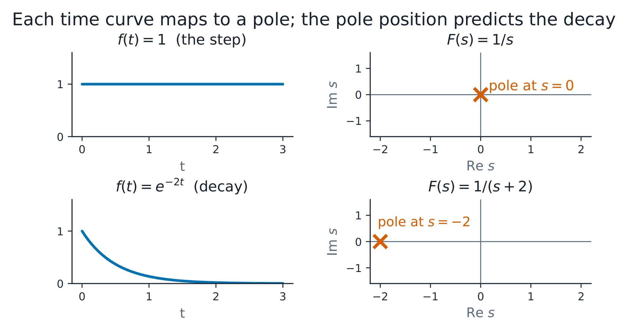
Each time curve maps to a pole; pole position predicts decay
Three working rules: $\mathcal{L}\{dy/dt\} = sY - y(0)$ (the initial condition
enters algebraically); $\mathcal{L}\{1\} = 1/s$; and partial fractions 部分分式
split a rational $F(s)$ into invertible pieces.
Worked example 1 (the unit-2.4 ODE, by transform). Solve $dy/dt + 2y = 10$,
$y(0) = 1$. Transformed: $sY - 1 + 2Y = 10/s$, so $Y = (10/s + 1)/(s + 2) =
10/[s(s+2)] + 1/(s+2)$. Partial fractions: $10/[s(s+2)] = 5/s - 5/(s+2)$. So
$Y = 5/s - 4/(s+2)$, and inverting term by term: $y = 5 - 4e^{-2t}$ — identical
to the classical route, with the initial condition handled by bookkeeping instead
of algebra at the end. The poles 极点 of $Y$ (here $s = 0, -2$) predict the
behaviour: a constant and a decaying exponential.
Worked example 2 (second order, machine-verified, escalated).$\frac{d^2y}
{dt^2} + 3\frac{dy}{dt} + 2y = 0$, $y(0) = 1$, $y'(0) = 0$. Transform:
$(s^{2} + 3s + 2)Y = s + 3$ (the derivative rule applied twice), so $Y =
\frac{s+3}{(s+1)(s+2)} = \frac{2}{s+1} - \frac{1}{s+2}$. Invert: $y = 2e^{-t} -
e^{-2t}$. Checks: $y(0) = 2 - 1 = 1$ ✓; $y'(0) = -2 + 2 = 0$ ✓; $y(1) = 0.736 -
0.135 = 0.600$ (machine-verified). The two poles $-1, -2$are the two decays,
with the slower pole $-1$ dominating the tail — the observation that later
courses turn into dominant-pole approximations.
Common mistakes. Forgetting the $-y(0)$ in the derivative rule (and its
second-order cousins $-y'(0) - s\,y(0)$). Inverting a $Y$ whose fractions are not
fully split: $\frac{s+3}{(s+1)(s+2)}$ must become two simple pieces before any
table lookup. Reading a zero at the numerator as a pole (a zero blocks; a pole
decays).
Summary: differentiation → multiplication by $s$, initials included; partial
fractions split $Y$; poles predict the time behaviour; the transform and
classical routes must agree — that agreement is the check.
A distorted mains waveform heats a resistor exactly as some combination of pure
sinusoids would — and which combination is not a guess but a computation. Any
periodic signal is a sum of sinusoids. For period $T$, fundamental 基波$ω_{0} = 2π/T$, the Fourier series 傅里叶级数 is
with each $a_{n}$, $b_{n}$ an average of $f$ against the matching sinusoid
(orthogonality 正交性: distinct sinusoids average to zero against each other —
so each coefficient can be picked out independently, like a bank of tuned
filters).
Odd harmonics 4/(nπ) build the square wave; the Gibbs overshoot never goes away
Worked example 1 (the square wave, verified at the magic point). A square
wave, ±1, period $T$, odd symmetry: all $a_{n} = 0$, and $b_{n} = 4/(nπ)$ for odd
$n$ — the series $\frac{4}{\pi}(\sin\omega_0 t + \frac{1}{3}\sin 3\omega_0 t +
\frac{1}{5}\sin 5\omega_0 t + \dots)$. The check that convinces: at $t = T/4$ the
sum must give 1, and $\frac{4}{\pi}(1 - \frac{1}{3} + \frac{1}{5} - \dots)$ is the
Gregory series for $π/4$ scaled — it converges to 1, exactly as the square wave
demands. Every harmonic 谐波 amplitude falls as $1/n$: sharper edges need more
harmonics, which is the whole of filtering.
Worked example 2 (power in the harmonics, machine-verified, escalated). A ±1 V
square wave across 1 Ω delivers average power 1 W (the mean of a constant
magnitude). Parseval says the harmonic powers must sum to the same 1 W:
$\sum_{n\ \text{odd}} \frac{1}{2}\big(\frac{4}{n\pi}\big)^{2} = \frac{8}{\pi^{2}}
\big(1 + \frac{1}{9} + \frac{1}{25} + \dots\big)$. Summing the first 20 odd
harmonics gives 0.990 W; the full series converges to 1 W exactly (the sum of
reciprocal odd squares is $π^{2}/8$, making the total
$\frac{8}{\pi^{2}}\cdot\frac{\pi^{2}}{8} = 1$). The practical reading: the
fundamental alone carries $\frac{8}{\pi^{2}} \approx 81\%$ of the power — a
low-pass filter that keeps only the first harmonic still delivers most of the
energy, and the 1/3-amplitude third harmonic adds just 9%.
Common mistakes. Using $n = T$ instead of $ω_0 = 2π/T$ as the fundamental
frequency. Forgetting the $\frac{1}{2}$ in each harmonic's power (a sinusoid's
mean square is half its peak square). Assuming even symmetry everywhere: shift
the origin and coefficients change — the spectrum belongs to the function as
placed.
Summary: periodic signals decompose into harmonics; orthogonality picks each
coefficient independently; amplitudes fall as $1/n$ for edges; Parseval audits
the power; the Gibbs overshoot never leaves.
Every measurement is noisy; the noise itself is a signal you cannot predict — but
its statistics are stable, and that stability is what instruments exploit. A
random variable 随机变量 has a probability distribution 概率分布; the
Gaussian (normal) $N(\mu, \sigma^{2})$ models thermal noise:
Expectation 期望$E[X]$ is the long-run average; variance 方差$Var(X) = E[X^{2}] - \mu^{2}$ is the spread, and $\sigma$ — the standard
deviation 标准差 — is the noise amplitude an oscilloscope shows. Two rules do
most of the work: independent variances add ($\sigma_{total} = \sqrt{\sigma_1^2 +
\sigma_2^2}$), and the average of $n$ independent samples has standard deviation
$\sigma/\sqrt{n}$.
Worked example 1 (the 2σ rule and averaging). For $X \sim N(0, \sigma^{2})$
with $\sigma = 2$ mV: $E[X] = 0$, $Var = 4$ (mV)², $\sigma = 2$ mV. The chance of
exceeding $\pm 2\sigma$ is 4.55% (the two-tailed 95% band is $\pm 1.96\sigma
\approx \pm 3.9$ mV). Averaging 16 independent samples yields $2/\sqrt{16} =
0.5$ mV of noise — the entire rationale of instrument averaging.
Worked example 2 (two noise sources, dB accounting, escalated). An amplifier
stage adds 2 mV of noise to a signal that already carries 3 mV from the previous
stage. The combined noise is not $3 + 2 = 5$ mV but
$\sqrt{3^{2} + 2^{2}} = \sqrt{13} = 3.61$ mV — variances add, not deviations, so
the smaller source contributes proportionally less than its face value.
Signal-to-noise improvement from averaging those same 16 readings:
$20\log_{10}(4) = 12.0$ dB. The design reading: four times the averaging buys 12
dB; fighting the dominant noise source at its origin buys more than any amount of
averaging — halving the 3 mV to 1.5 mV would give
$\sqrt{1.5^{2} + 2^{2}} = 2.5$ mV, a 3.2 dB improvement for free.
Common mistakes. Adding standard deviations instead of variances. Confusing
$\sigma$ and $\sigma^{2}$ in tables and formulas (the scope shows σ; formulas
usually use σ²). Forgetting that $\sigma/\sqrt{n}$ improvement assumes
independence — correlated noise (mains hum) does not average away.
Summary: the Gaussian is the noise model; σ is the scope's noise; independent
variances add, averaging divides σ by √n; attack the dominant source, then
average.
probability distribution/ˌprɒbəˈbɪlɪti ˌdɪstrɪˈbjuːʃn/
概率分布
gài lǜ fēn bù
expectation/ekspɪkˈteɪʃn/
期望
qī wàng
variance/ˈveərɪəns/
方差
fāng chà
standard deviation/ˈstændəd ˌdiːvɪˈeɪʃn/
标准差
biāo zhǔn chà
2.8
向量微积分
English
A voltage probe reports one number at each point in space — a whole landscape of
values, and EE07's Maxwell equations are statements about that landscape's
geometry. Fields are vector-valued functions of position. Three operators on a
field $\mathbf{F}$:
Gradient 梯度$\nabla V$: points up the steepest slope of a scalar; the
electric field is $E = -\nabla V$.
Divergence 散度$\nabla \cdot \mathbf{F}$: the net outflow per unit volume —
charge density for electric fields.
Curl 旋度$\nabla \times \mathbf{F}$: the circulation per unit area — zero
for electrostatics, the mechanism of induction where it is not.
Read a field's story at a glance: outflow means divergence, swirl means curl
Worked example 1 (the gradient predicts the drop, verified numerically).$V(x, y) = 3x^{2}y$ volts. $\nabla V = (6xy, 3x^{2})$; at the point $(1, 2)$:
$\nabla V = (12, 3)$, so $E = -(12, 3)$ V/m. The check: move a small step
$\delta = (0.01, 0)$ from $(1, 2)$ — $V$ changes by $\approx 6xy\cdot\delta x =
12 \times 0.01 = 0.12$ V, and $-E\cdot\delta = 12 \times 0.01 = 0.12$ V: the
field times the step predicts the potential drop, which is what gradient means.
Worked example 2 (divergence and curl by hand, escalated). For
$\mathbf{F} = (x^{2},\ xy,\ 3x^{2}z)$: $\nabla\cdot\mathbf{F} = 2x + x + 3x^{2}$,
which at $(1,1,1)$ equals $2 + 1 + 3 = 6$ — a net source. For the circulating field
$\mathbf{G} = (-y,\ x,\ 0)$: the $z$-component of curl is
$\frac{\partial G_y}{\partial x} - \frac{\partial G_x}{\partial y} = 1 - (-1) = 2$ —
uniform rotation of strength 2 everywhere: the velocity field of a rigid
body spinning at 1 rad/s, whose curl is twice its angular velocity. These two computations are the pointwise versions of
EE07's Gauss and Stokes laws.
Common mistakes. Taking the gradient of a vector or the divergence of a
scalar — gradient is for scalars, divergence for vectors. Sign slips in curl:
the $z$-component is $\partial F_y/\partial x - \partial F_x/\partial y$; reversing them
flips the rotation. A uniform field has zero divergence AND zero curl.
Summary: gradient is steepest-up (scalar→vector), divergence is net outflow
(vector→scalar), curl is circulation (vector→vector); a step must reconcile
$E \cdot \delta$ with $\delta V$.