This is the sixth course in University Electrical Engineering: signals and
systems 信号与系统. EE04 asked "what does THIS circuit do at THIS frequency";
this course asks the deeper question: what does a system do to ANY input —
answered through the three transforms (convolution, Fourier, z) that the rest of
the degree (communications, DSP, control) is built on.
Unit 6.1 classifies signals and systems.
Unit 6.2 makes convolution the universal time-domain answer.
Units 6.3–6.4 move to frequency: Fourier series/transforms and sampling.
Unit 6.5 reuses EE02's Laplace machinery as the system function.
Units 6.6–6.7 go discrete: difference equations and the z-transform.
The running story is one audio channel: a microphone signal, a filter, a
sampler, a digital equaliser. Every transform below moves that channel
forward, and every answer is checked the way a signals engineer checks it —
by deriving each transform pair at least once, verifying every convolution
two ways (graphically and by the Fourier product when available), and
testing every discrete result by direct iteration.
Why it matters. "Is it linear? Is it time-invariant?" are the first two
questions of every analysis in this course — the answers decide which of
all the machinery is even allowed.
The idea, with a picture. A signal 信号 is a function of time:
continuous-time $x(t)$ or discrete-time $x[n]$. A system 系统 maps input
signals to output signals. Four properties carry the course, and each is a
test you run on ONE carefully chosen input, not a feeling:
Linearity 线性: $ax_{1} + bx_{2} \to ay_{1} + by_{2}$ — feed the sum,
check the sum of the outputs.
Time invariance 时不变性: shift the input by $T$; the output must shift
by exactly $T$ and nothing else.
Causality 因果性: the output at time $t$ depends only on $x$ up to $t$.
BIBO stability BIBO 稳定性: every bounded input gives a bounded
output; for an LTI system this collapses to
$\int |h(t)|\,dt < \infty$ — the impulse response must be absolutely
integrable.
Each property is one experiment: pick the probe input, compare the two outputs
The derivation. Time invariance fails whenever the system's clock
scales: for $y(t) = x(2t)$, shifting the input by $T$ gives
$y_{shift}(t) = x(2t - T) = x(2(t - T/2))$ — the output is the original
system's output delayed by only $T/2$. Comparing "shift then system"
($x(t-T) \to y(t)$ at argument $2t$, i.e. $x(2t - T)$) against
"system then shift" ($y(t - T) = x(2t - 2T)$) exposes the mismatch
whenever it exists — that comparison IS the test.
Worked example 1 — the time-scaling trap. Is $y(t) = x(2t)$
time-invariant? With $x(t) = u(t)$: shift-then-system gives
$x(t-1) = u(t-1) \to u(2t-1) = u(t - \tfrac{1}{2})$; system-then-shift
gives $y(t-1) = u(2(t-1)) = u(t-1)$. Half shift versus full shift —
time-varying ✓. A 2× fast-playback stage in the running audio channel
fails exactly this way.
Worked example 2 — stability by the integral. The channel's room-echo
model $h(t) = e^{-t}u(t)$: $\int_{0}^{\infty} e^{-t}\,dt = 1 < \infty$ ✓
stable. The same filter with $h(t) = u(t)$ (an integrator) gives
$\int_{0}^{\infty} 1\,dt = \infty$ — a bounded step input produces an
unbounded ramp output, so the integrator is BIBO-unstable however harmless it
looks. One integral, one verdict.
Common mistakes. Testing linearity with one input (you need two, plus
scaling). Declaring time invariance from a diagram (run the shift test).
And confusing causality with stability: $h(t) = e^{-t}u(t)$ is both, but
$h(t) = -e^{t}u(-t)$ (anti-causal, decaying) is stable and NOT causal —
the two properties are independent.
Summary. Linearity + time invariance unlock convolution; causality
orders cause and effect; BIBO stability is $\int|h| < \infty$. Every
property is a one-probe experiment.
Why it matters. Convolution is the ONE formula that gives the output
of any linear time-invariant system to ANY input — no transform, no
transfer function, just the impulse response and an integral.
The idea, with a picture. For a linear time-invariant 线性时不变
system, the impulse response 冲激响应$h(t)$ determines everything:
decompose the input into delayed, scaled impulses; each impulse
$\delta(t-\tau)\,x(\tau)\,d\tau$ produces $h(t-\tau)$ scaled; superposition
integrates them all:
Convolution 卷积 is slide–multiply–integrate: flip $h$, slide it past
$x$, and each output value is the area of the overlap.
Each value of y(t) is the overlap area as h slides past x
The derivation. Sifting: $x(t) = \int x(\tau)\delta(t-\tau)\,d\tau$.
Linearity moves the integral outside; time invariance turns
$\delta(t-\tau) \to h(t-\tau)$; the result is the convolution integral —
three properties, one formula.
Worked example 1 — the classic step response. The channel's filter
$x(t) = u(t)$ into $h(t) = e^{-t}u(t)$: for $t \ge 0$ the overlap is
$\tau \in [0, t]$, so
Check the ends: $y(0) = 0$ ✓ (no output before any input arrives);
$y(\infty) = 1$ ✓ (DC gain 1 — and indeed $H(0) = 1$). At $t = 1.5$,
$y = 1 - e^{-1.5} = 0.777$ — the shaded overlap area in the figure.
Worked example 2 — escalate to the pulse. Now a 2-second rectangular
input of height 1 (a held note) into the same filter. Two checkpoints by
superposition: the step ON at $t=0$ plus a step OFF at $t=2$, so
$y(t) = (1 - e^{-t})u(t) - (1 - e^{-(t-2)})u(t-2)$. At $t = 1$:
$1 - e^{-1} = 0.632$. At $t = 3$: $(1 - e^{-3}) - (1 - e^{-1}) =
e^{-1} - e^{-3} = 0.318$ — the release tail. Check the peak at
$t = 2^-$: $1 - e^{-2} = 0.865$, and at $t = 2^+$ the second term
subtracts exactly its start, so the curve is continuous with a slope
discontinuity of $-1$ — the kink the ear hears as the note-off.
Common mistakes. Forgetting the flip (convolution is NOT
$\int x(\tau)h(\tau)\,d\tau$). Dropping the limits when the signals start
at 0 (the overlap window, not $(-\infty,\infty)$, does the work). And
assuming $x * h = x \cdot h$ — multiplication is what happens in the
FREQUENCY domain, never in time.
Summary.$y = x * h$; flip, slide, integrate; widths add
($W_{1} + W_{2}$); commutative; cascades convolve. Every transform later
exists to avoid doing this integral.
Why it matters. The channel's noise, its harmonics, its equaliser
bands — all live in frequency. The Fourier transform is the bridge, and
its convolution-to-multiplication property is why filters are designed
there.
The idea, with a picture. Periodic signals expand into harmonics
(EE02's series); the Fourier transform 傅里叶变换 extends the idea to
aperiodic signals:
the sinc function. At $\omega = 0$ the transform equals the AREA $A\tau$
(and $\mathrm{sinc}(0) = 1$ returns it ✓); the first null sits at
$\omega\tau/2 = \pi$, i.e. $f = 1/\tau$ — the time–bandwidth trade-off时间带宽权衡.
Worked example 1 — the channel's pulse budget. A 1 ms click
($A = 1$, $\tau = 10^{-3}$ s): $X(f) = 10^{-3}\,\mathrm{sinc}(f \cdot 10^{-3})$,
first null at $f = 1$ kHz. A ten-times-shorter click (0.1 ms) pushes the
null to 10 kHz — the shorter the event, the wider the spectrum, which is
why a click irritates every band of the equaliser at once. Check the
area: the value at $f = 0$ is $A\tau$ — $10^{-3}$ for the 1 ms click and
$10^{-4}$ for the 0.1 ms one ✓; the shorter click puts less into each band
but spreads it over ten times as many.
Worked example 2 — escalate to the ideal filter's price. The channel
wants a brick-wall low-pass: gain 1 to 4 kHz, 0 above. Its impulse
response is the inverse transform of the passband rectangle:
$h(t) = \frac{\sin(\omega_{c}t)}{\pi t}$ with
$f_{c} = 4$ kHz — a sinc in TIME, stretching infinitely in both
directions, so the ideal filter is non-causal. Truncate it to
$|t| \le 5$ ms (a 10 ms window) and the passband gains ripple (Gibbs),
with ripples about $1/(10\ \text{ms}) = 100$ Hz apart, and the edge can be
no sharper than about that same 100 Hz. The trade-off is honest:
steepness in frequency is paid in time-domain length, the same law from
the other side.
Common mistakes. Evaluating $\mathrm{sinc}$ at $\omega$ rather than
$\omega\tau/2$ (dimensionless argument, always). Forgetting the $1/2\pi$
on the inverse. And reading $|X(\omega)|$ as "the signal" — the transform
is complete only with its phase.
Summary. Transform pairs by the integral; pulse ↔ sinc with null at
$1/\tau$; convolution ↔ multiplication. Steepness in one domain is length
in the other.
Why it matters. The channel goes digital at one point: the sampler.
Everything downstream — the equaliser, the storage, the reconstruction —
inherits whatever the sampling step did, and it can never be undone
afterwards.
The idea, with a picture. Sampling multiplies the signal by an
impulse train; in frequency, the spectrum replicates at multiples of
$f_{s}$. The Nyquist criterion 奈奎斯特准则: a signal band-limited to
$f_{max}$ is perfectly recoverable if $f_{s} > 2f_{max}$. Below that,
replicas overlap and aliasing 混叠 folds high frequencies into the
band as false lows.
Sampled at 6 kHz, a 4 kHz tone is indistinguishable from 2 kHz
The derivation. A sampler output
$x_{s}(t) = x(t)\sum_{n}\delta(t - nT)$ has, by the convolution-to-
multiplication duality (multiplication in time = convolution in
frequency), the spectrum $(1/T)\sum_{k} X(\omega - k\omega_{s})$ —
replicas at every multiple of the sampling frequency. If
$X$ occupies $|\omega| < \omega_{s}/2$, the replicas never touch; any
narrower spacing overlaps them, and within the overlap no filter can tell
a true low frequency from a folded high one.
Worked example 1 — the 4 kHz alias. A 4 kHz sine sampled at 6 kHz:
$4 > 6/2 = 3$, so the sequence is indistinguishable from
$|f - f_{s}| = 2$ kHz. Check sample by sample:
$\cos(2\pi \cdot \tfrac{4}{6} n) = \cos(2\pi \cdot \tfrac{2}{3} n)$ and
$\cos(2\pi \cdot \tfrac{2}{6} n) = \cos(2\pi \cdot \tfrac{1}{3} n)$;
the two sequences agree because
$\cos(2\pi \cdot \tfrac{2}{3} n) = \cos(2\pi(\tfrac{2}{3} - 1)n) =
\cos(2\pi \cdot (-\tfrac{1}{3})n) = \cos(2\pi \cdot \tfrac{1}{3} n)$ ✓
(cosine is even). A 4 kHz tone sampled at 6 kHz IS a 2 kHz sequence.
Worked example 2 — escalate to the anti-alias budget. The channel's
microphone carries content to 20 kHz; the sampler runs at 44.1 kHz
($f_{s}/2 = 22.05$ kHz). A 23 kHz interference tone would alias to
$44.1 - 23 = 21.1$ kHz — audible. The anti-alias filter 抗混叠滤波器
must cut it before the sampler: at 44.1 kHz CD sampling the guard band is
only 22.05 − 20 = 2.05 kHz wide, which is why professional capture
oversamples at 96 or 192 kHz (guard bands of 28 and 76 kHz) and filters
gently. The fix is always before the sampler, never after — a folded
frequency carries no flag saying where it came from.
Common mistakes. Counting $f_{s} = 2f_{max}$ as safe (the inequality
is strict; at equality a sine at $f_{max}$ can be sampled at its zero
crossings and vanish). Filtering after sampling (the
fold is already inside the band). And assuming digital upsampling
recovers what a low $f_{s}$ missed — the information was never recorded.
Summary. Sampling replicates the spectrum at $f_{s}$;
$f_{s} > 2f_{max}$ or aliases fold; the anti-alias filter goes before the
sampler; the guard band between $f_{max}$ and $f_{s}/2$ is the design
budget.
Why it matters. The channel's analogue stage — coupling capacitors,
tone controls — is a rational system, and the poles of its system
function predict ringing, speed and stability at a glance.
The idea, with a picture. EE02's Laplace transform becomes the
system function 系统函数$H(s) = Y(s)/X(s)$; for an LTI system,
$h(t) \leftrightarrow H(s)$ as a transform pair. Rational $H(s)$ factors
into poles and zeros 零极点: each pole contributes a natural mode
$e^{pt}$; the region of convergence (ROC) decides which; causal
stability requires all poles in the open left half-plane.
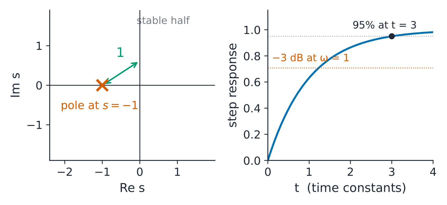
One pole at −1: the decay rate in time, the −3 dB frequency in the response — one number, three readings
The derivation.$\mathcal{L}\{e^{-at}u(t)\} = 1/(s+a)$ for
$\mathrm{Re}(s) > -a$ (one integration by parts). The unit step
$1/s$. So for $H(s) = 1/(s+1)$ driven by a step:
partial fractions doing the convolution of Unit 6.2 with three lines of
algebra — and both routes land on the same curve ✓.
Worked example 1 — read the pole three ways.$H(s) = 1/(s+1)$: the
pole at $s = -1$ IS the $e^{-t}$ in the impulse response (time constant
1 s); the step response settles at $1 - e^{-t}$ reaching 95% at
$t = 3$ s; the frequency response 频率响应$H(j\omega)$ has
$|H(j \cdot 1)| = 1/\sqrt{2} = 0.707$ — the −3 dB point sits exactly at
the pole's distance from the origin, and the phase there is $-45°$.
Worked example 2 — escalate to the two-pole tone control. A bass
boost with a notch, $H(s) = \dfrac{s^{2} + 2s + 100}{(s+1)(s+10)}$: zeros at
$-1 \pm j9.95$ (close to the imaginary axis near $\pm 10$ rad/s, so they
carve a notch there: $|H(j10)| = 20/(10.05 \times 14.14) = 0.14$, about
−17 dB), poles at $-1$ and $-10$ (both left — stable ✓). DC gain
$100/10 = 10$ (20 dB of bass lift ✓); high-frequency gain
$1$ (the numerator's $s^{2}$ matches the denominator's). Check the
mid-dip: at $\omega = 0$, 20 dB; at $\omega \to \infty$, 0 dB; the
transition lives between the pole frequencies — the whole equaliser curve
is legible from five marked points on the s-plane.
Common mistakes. Reading stability from the poles without the ROC
(a pole at $-1$ with a left-extending ROC is anti-causal and unstable).
Forgetting $H(s)$ only exists with its ROC. And trusting a pole-zero
plot scaled wrong: the −3 dB point is the pole's DISTANCE from the
origin only for a first-order factor with no nearby zeros.
Summary.$H(s) = Y/X$; partial fractions turn transforms back into
exponentials; poles set the modes, the ROC the causality, the left
half-plane the stability, and $s = j\omega$ the frequency response.
Why it matters. Once sampled, the channel's equaliser is a difference
equation running on a processor — iterating it by hand is how its
behaviour is actually understood.
The idea, with a picture. The discrete mirror of convolution:
$y[n] = \sum_{k} x[k]\,h[n-k]$. Systems described by difference
equations 差分方程 such as $y[n] = 0.5\,y[n-1] + x[n]$ — an accumulator
with decay. The homogeneous mode is $a^{n}$ where $a$ is the root of the
characteristic equation; iterating one step at a time is the direct
solution.
Each step halves the remaining gap to the limit — a geometric approach you can verify on your fingers
The derivation. For $y[n] = a\,y[n-1] + x[n]$ with step input and
zero initial condition, the first samples are
$1,\ 1+a,\ 1+a+a^{2},\ \ldots$ — partial sums of a geometric series, so
and the limit $1/(1-a)$ is the DC gain: the discrete echo of the
continuous $\int h < \infty$ condition.
Worked example 1 — iterate and converge.$y[n] = 0.5y[n-1] + x[n]$,
$y[-1] = 0$, unit step: $y[0] = 1$, $y[1] = 1.5$, $y[2] = 1.75$,
$y[3] = 1.875$ — closing on the DC gain $1/(1-0.5) = 2$ ✓. The gap to
the limit halves each step (the residue is $0.5^{n+1}$), so after 10
steps the gap is $0.5^{11} \approx 0.05\%$ — one line of arithmetic
predicting the whole table.
Worked example 2 — escalate to an oscillating root. Set
$a = -0.8$: $y[n] = -0.8\,y[n-1] + x[n]$ on a step gives
$y[n] = \tfrac{1}{1.8}(1 - (-0.8)^{n+1})$ — the approach to
$0.556$ oscillates: $y[0] = 1$, $y[1] = 0.2$, $y[2] = 0.84$,
$y[3] = 0.328$. Check $|a| = 0.8 < 1$ — still stable (the oscillation
decays), and the sign flips every sample are the fingerprint of a
negative root, the discrete analogue of a complex pole pair near the
imaginary axis.
Common mistakes. Iterating with a wrong $y[-1]$ (state the initial
condition before the first line). Declaring stability from the first few
samples (only $|a| < 1$ decides). And reading the DC gain from $n = 0$
alone — it is $1/(1-a)$, the LIMIT, visible only as the samples settle.
Summary. Difference equation → iterate; geometric partial sums;
DC gain $1/(1-a)$; root inside the unit circle = stability; negative or
complex roots = oscillation.
6.7
Z变换
English
Why it matters. The equaliser ships as coefficients
$a_{k}, b_{k}$ of a difference equation; the z-transform is how those
numbers are chosen, and the unit circle 单位圆 is where their frequency response
is read off.
The idea, with a picture. The z-transform z 变换$X(z) = \sum_{n} x[n]z^{-n}$ plays Laplace's role in discrete time. The
fundamental pair: $a^{n}u[n] \leftrightarrow 1/(1 - az^{-1})$ with ROC
$|z| > |a|$. Poles INSIDE the unit circle mean stability, and the
inverse transform is long division or partial fractions.
The unit circle is the frequency axis; the pole radius is the damping — one picture joins the two domains
The derivation.$\sum_{n=0}^{\infty} a^{n}z^{-n}$ is geometric with
ratio $az^{-1}$; it converges to $1/(1 - az^{-1})$ exactly when
$|az^{-1}| < 1$, i.e. $|z| > |a|$ — the ROC is the exterior of a circle
through the pole. Stability needs the ROC to include the unit circle
(the frequency axis $z = e^{j\omega}$), which forces $|a| < 1$ — the
unit-circle condition in one line.
Worked example 1 — the accumulator again, by transform.$H(z) = 1/(1 - 0.5z^{-1})$, pole at $z = 0.5$ — inside the unit circle,
stable ✓. Step response:
$Y(z) = H(z)\,\dfrac{z}{z-1} = \dfrac{z^{2}}{(z-0.5)(z-1)}$; partial
fractions give $y[n] = 2(1 - 0.5^{n+1})$. Check $n = 0$: $2(1 - 0.5) = 1$
✓ matches the iteration of Unit 6.6, and $n \to \infty$ gives
$2$ ✓ — the DC gain again. Two methods, one sequence.
Worked example 2 — the plane-to-plane dictionary. The mapping
$s \to z = e^{sT}$ sends $s = j\omega$ to the unit circle
$e^{j\omega T}$ (frequency = angle), and a continuous decay rate
$\sigma$ to a radius $e^{\sigma T}$. The accumulator's pole at
$z = 0.5$ with $T = 1$ ms corresponds to
$\sigma = \ln(0.5)/0.001 = -693\ \text{s}^{-1}$ — a time constant of
$1/693 = 1.44$ ms. Check against Unit 6.6's iteration: the gap halves
per SAMPLE ($0.5 = e^{-0.693}$), and $0.693/T$ per second is the same
$-693\ \text{s}^{-1}$ ✓. The two transforms are one subject seen from
two banks of the same river.
Common mistakes. Quoting $H(z)$ without its ROC (the same rational
function belongs to three different systems). Reading frequency response
off the real axis (it lives on $|z| = 1$). And confusing $z$ and
$z^{-1}$ conventions — with $z^{-1}$ as the delay, a pole at $|a|$
converges only for $|z| > |a|$.
Summary.$a^{n} \leftrightarrow 1/(1-az^{-1})$, ROC exterior;
poles inside the unit circle = stability; $z = e^{sT}$ maps decay to
radius and frequency to angle — and the DC gain $1/(1-a)$ closes the
loop with the iteration two units ago.