Skip to content · ⁨ข้ามไปยังเนื้อหา⁩
Subjects · ⁨รายวิชา⁩

AP Precalculus

Tips · ⁨เคล็ดลับ⁩

AP Precalculus ครอบคลุม ฟังก์ชันพหุนามและฟังก์ชันเศษส่วน, ฟังก์ชันเอ็กซ์โพเนนเชียลและลอการิทึม, ฟังก์ชันตรีโกณมิติและขั้ว, และการแนะนำเกี่ยวกับ เวกเตอร์ เมทริกซ์ และฟังก์ชันพารามิเตอร์ เป็นสะพานเชื่อมเข้าสู่แคลคูลัส และข้อสอบเข้มงวดเป็นพิเศษเกี่ยวกับ วิธีการอธิบายฟังก์ชันของคุณ

การอธิบายการเปลี่ยนแปลงคือหัวใจของหลักสูตรทั้งหมด คาดว่าจะต้องระบุ จุดที่ฟังก์ชันเพิ่มขึ้นหรือลดลง, ด้วยความเร็วเท่าไร, และ อัตราการนั้นเองก็เพิ่มขึ้นหรือไม่ — เป็นประโยคสมบูรณ์พร้อมใช้คำศัพท์ที่ถูกต้อง

จำ parent functions และการแปลงต่างๆ ได้ดี ทุกอย่างในหลักสูตรสร้างจากสิ่งเหล่านี้ และการจดจำ parent function ที่ถูกเลื่อนหรือยืดขยายได้ทันที คือสิ่งที่ทำให้ข้อยากๆ กลายเป็นข้อสั้น

หมายเหตุเรียงตามสี่หน่วย CED — พหุนามและเศษส่วน, เอ็กซ์โพเนนเชียลและลอการิทึม, ตรีโกณมิติและขั้ว, และฟังก์ชันที่มีพารามิเตอร์ — แต่ละหน่วยมีตัวอย่างเฉลย ตัวอย่าง ข้อสอบ วางอยู่ในห้องสมุด PreCalculus要求你用句子描述函数的行为,示例对此进行了示范。

  • 1

    Polynomial and Rational Functions · ⁨ฟังก์ชันพหุนามและฟังก์ชันอัตราส่วน⁩

    Watch lesson · ⁨ดูบทเรียน⁩
    1.1

    Change in Tandem · ⁨การเปลี่ยนแปลงแบบคู่⁩

    Syllabus · ⁨หลักสูตร⁩
    English

    Learning Objective 1.1.A: Describe how the input and output values of a function vary together by comparing function values.

    • 1.1.A.1 A function is a mathematical relation that maps a set of input values to a set of output values such that each input value is mapped to exactly one output value. The set of input values is called the domain of the function, and the set of output values is called the range of the function. The variable representing input values is called the independent variable, and the variable representing output values is called the dependent variable.
    • 1.1.A.2 The input and output values of a function vary in tandem according to the function rule, which can be expressed graphically, numerically, analytically, or verbally.
    • 1.1.A.3 A function is increasing over an interval of its domain if, as the input values increase, the output values always increase. That is, for all $a$ and $b$ in the interval, if $a < b$, then $f(a) < f(b)$.
    • 1.1.A.4 A function is decreasing over an interval of its domain if, as the input values increase, the output values always decrease. That is, for all $a$ and $b$ in the interval, if $a < b$, then $f(a) > f(b)$.

    Learning Objective 1.1.B: Construct a graph representing two quantities that vary with respect to each other in a contextual scenario.

    • 1.1.B.1 The graph of a function displays a set of input-output pairs and shows how the values of the function's input and output values vary.
    • 1.1.B.2 A verbal description of the way aspects of phenomena change together can be the basis for constructing a graph.
    • 1.1.B.3 The graph of a function is concave up on intervals in which the rate of change is increasing.
    • 1.1.B.4 The graph of a function is concave down on intervals in which the rate of change is decreasing.
    • 1.1.B.5 The graph intersects the $x$-axis when the output value is zero. The corresponding input values are said to be zeros of the function.
    ไทย

    วัตถุประสงค์การเรียนรู้ 1.1.A: อธิบายว่าค่าอินพุตและเอาต์พุตของฟังก์ชันเปลี่ยนแปลงร่วมกันอย่างไรโดยการเปรียบเทียบค่าฟังก์ชัน

    • 1.1.A.1 ฟังก์ชัน คือความสัมพันธ์ทางคณิตศาสตร์ที่จับคู่เซตของค่าอินพุตเข้ากับเซตของค่าเอาต์พุต โดยที่ค่าอินพุตแต่ละค่าถูกจับคู่กับค่าเอาต์พุตเพียงค่าเดียว เซตของค่าอินพุตเรียกว่า โดเมน ของฟังก์ชัน และเซตของค่าเอาต์พุตเรียกว่า เรนจ์ ของฟังก์ชัน ตัวแปรที่แทนค่าอินพุตเรียกว่า ตัวแปรอิสระ และตัวแปรที่แทนค่าเอาต์พุตเรียกว่า ตัวแปรตาม
    • 1.1.A.2 ค่าอินพุตและเอาต์พุตของฟังก์ชันเปลี่ยนแปลงแบบคู่ขนานตาม กฎฟังก์ชัน ซึ่งสามารถแสดงออกได้ทั้งในรูปแบบกราฟ จำนวน สมการ หรือคำบรรยาย
    • 1.1.A.3 ฟังก์ชันเป็นฟังก์ชันเพิ่มบนช่วงหนึ่งของโดเมนได้ หากเมื่อค่าอินพุตเพิ่มขึ้น ค่าเอาต์พุตจะเพิ่มขึ้นเสมอ นั่นคือ สำหรับทุก $a$ และ $b$ ในช่วงนั้น หาก $a < b$ แล้ว $f(a) < f(b)$
    • 1.1.A.4 ฟังก์ชันจะลดลงในช่วงหนึ่งของโดเมนของมันหาก เมื่อค่าอินพุตเพิ่มขึ้น ค่าเอาต์พุตจะลดลงเสมอ นั่นคือ สำหรับทุก $a$ และ $b$ ในช่วงนั้น หาก $a < b$ แล้ว $f(a) > f(b)$

    วัตถุประสงค์การเรียนรู้ 1.1.B: สร้างกราฟที่แสดงความสัมพันธ์ระหว่างสองปริมาณที่แปรผันต่อกันในสถานการณ์ที่มีบริบท

    • 1.1.B.1 กราฟของฟังก์ชันแสดงคู่ค่าอินพุต-เอาต์พุตและชี้ให้เห็นถึงการเปลี่ยนแปลงของค่าอินพุตและเอาต์พุตของฟังก์ชัน
    • 1.1.B.2 คำบรรยายด้วยภาษาธรรมชาติเกี่ยวกับวิธีการที่องค์ประกอบต่างๆ ของปรากฏการณ์เปลี่ยนแปลงร่วมกัน สามารถใช้เป็นพื้นฐานในการสร้างกราฟ
    • 1.1.B.3 กราฟของฟังก์ชันมีลักษณะ เว้าขึ้น (concave up) บนช่วงที่อัตราการเปลี่ยนแปลงเพิ่มขึ้น
    • 1.1.B.4 กราฟของฟังก์ชันมีลักษณะ เว้าลง (concave down) บนช่วงที่อัตราการเปลี่ยนแปลงลดลง
    • 1.1.B.5 กราฟตัดแกน $x$ เมื่อค่าเอาต์พุตเป็นศูนย์ ค่าอินพุตที่เกี่ยวข้องกันนี้เรียกว่า รากของฟังก์ชัน (zeros of the function)

    Source: College Board AP Course and Exam Description · ⁨แหล่งที่มา: คำอธิบายหลักสูตรและข้อสอบ College Board AP⁩

    English

    A function 函数 is a rule that maps each input to exactly one output. The set of allowed inputs is the domain 定义域; the set of outputs is the range 值域. The input variable is the independent variable 自变量 and the output variable is the dependent variable 因变量. A function rule can be shown graphically, numerically, analytically (a formula), or verbally.

    As the input changes, the output changes "in tandem" – together. Over an interval, a function is:

    • increasing 递增 if, whenever $a, then $f(a) (bigger input, bigger output);
    • decreasing 递减 if, whenever $a, then $f(a)>f(b)$ (bigger input, smaller output).

    A graph of a function shows all its input–output pairs, so you can read this behavior straight off the picture.

    ไทย

    ฟังก์ชัน คือกฎที่จับคู่อินพุตแต่ละตัวเข้ากับ เอาต์พุตเพียงหนึ่งเดียว เซตของอินพุตที่เป็นไปได้เรียกว่า โดเมน; เซตของเอาต์พุตคือ เรนจ์ ตัวแปรอินพุตคือ ตัวแปรอิสระ และตัวแปรเอาต์พุตคือ ตัวแปรขึ้นกับ กฎของฟังก์ชันสามารถแสดงได้ทั้งแบบกราฟ, แบบตารางข้อมูล, แบบวิเคราะห์ (ด้วยสูตร) หรือแบบคำบรรยาย

    เมื่ออินพุตเปลี่ยนแปลง เอาต์พุตก็เปลี่ยน "ตามไปด้วย" – พร้อมกัน ในช่วงหนึ่ง ฟังก์ชันจะเป็น:

    • เพิ่มขึ้น หากว่าทุกครั้งที่ $a แล้ว $f(a) (อินพุตใหญ่ขึ้น เอาต์พุต也大);
    • ลดลง หากว่าทุกครั้งที่ $a แล้ว $f(a)>f(b)$ (อินพุตใหญ่ขึ้น เอาต์พุตเล็กลง).

    กราฟของฟังก์ชันจะแสดงคู่ค่าอินพุต-เอาต์พุตทั้งหมด ทำให้คุณสามารถอ่านพฤติกรรมนี้ได้โดยตรงจากภาพ

    Explore · ⁨สำรวจ⁩

    Watch two quantities change together · ⁨สังเกตการเปลี่ยนแปลงร่วมกันของปริมาณสองอย่าง⁩

    y = ax² + bx + c

    Precalculus studies how an output changes in tandem with its input. Read the curve left to right: where it is steep, $y$ changes a lot for a small change in $x$; where it is flat, $y$ barely moves. · ⁨แคลคูลัสก่อนเรียนศึกษาว่าเอาต์พุตเปลี่ยนแปลง พร้อมกัน กับอินพุตอย่างไร อ่านcurve从左至右:的地方 steep, $y$ เปลี่ยนแปลงมากสำหรับการเปลี่ยนแปลงเล็กน้อยใน $x$;的地方 flat, $y$ แทบไม่เคลื่อนที่⁩

    1.2

    Rates of Change · ⁨อัตราการเปลี่ยนแปลง⁩

    Syllabus · ⁨หลักสูตร⁩
    English

    Learning Objective 1.2.A: Compare the rates of change at two points using average rates of change near the points.

    • 1.2.A.1 The average rate of change of a function over an interval of the function's domain is the constant rate of change that yields the same change in the output values as the function yielded on that interval of the function's domain. It is the ratio of the change in the output values to the change in input values over that interval.
    • 1.2.A.2 The rate of change of a function at a point quantifies the rate at which output values would change were the input values to change at that point. The rate of change at a point can be approximated by the average rates of change of the function over small intervals containing the point, if such values exist.
    • 1.2.A.3 The rates of change at two points can be compared using average rate of change approximations over sufficiently small intervals containing each point, if such values exist.

    Learning Objective 1.2.B: Describe how two quantities vary together at different points and over different intervals of a function.

    • 1.2.B.1 Rates of change quantify how two quantities vary together.
    • 1.2.B.2 A positive rate of change indicates that as one quantity increases or decreases, the other quantity does the same.
    • 1.2.B.3 A negative rate of change indicates that as one quantity increases, the other decreases.
    ไทย

    วัตถุประสงค์การเรียนรู้ 1.2.A: เปรียบเทียบอัตราการเปลี่ยนแปลงที่จุดสองจุดโดยใช้อัตราการเปลี่ยนแปลงเฉลี่ยใกล้จุดเหล่านั้น

    • 1.2.A.1 อัตราการเปลี่ยนแปลงเฉลี่ยของฟังก์ชันในช่วงหนึ่งของโดเมนฟังก์ชันคืออัตราการเปลี่ยนแปลงคงที่ซึ่งจะให้ค่าการเปลี่ยนแปลงในค่าเอาต์พุตเท่ากับการเปลี่ยนแปลงที่ฟังก์ชันให้ไว้ในช่วงนั้นของโดเมนฟังก์ชัน เป็นอัตราส่วนของการเปลี่ยนแปลงในค่าเอาต์พุตต่อการเปลี่ยนแปลงในค่าอินพุตในช่วงนั้น
    • 1.2.A.2 อัตราการเปลี่ยนแปลงของฟังก์ชันที่จุดหนึ่งวัดปริมาณอัตราการเปลี่ยนแปลงที่ค่าเอาต์พุตจะเปลี่ยนไปหากค่าอินพุตเปลี่ยนไป ณ จุดนั้น อัตราการเปลี่ยนแปลงที่จุดหนึ่งสามารถประมาณได้โดยใช้อัตราการเปลี่ยนแปลงเฉลี่ยของฟังก์ชันในช่วงเล็กๆ ที่รวมจุดนั้นไว้ หากมีค่าดังกล่าว
    • 1.2.A.3 อัตราการเปลี่ยนแปลงที่จุดสองจุดสามารถเปรียบเทียบได้โดยใช้ค่าประมาณอัตราการเปลี่ยนแปลงเฉลี่ยในช่วงเล็กๆ เพียงพอที่รวมแต่ละจุดไว้ หากมีค่าดังกล่าว

    วัตถุประสงค์การเรียนรู้ 1.2.B: อธิบายว่าปริมาณสองชนิดแปรผันร่วมกันอย่างไรที่จุดต่างๆ และในช่วงต่างๆ ของฟังก์ชัน

    • 1.2.B.1 อัตราการเปลี่ยนแปลงวัดปริมาณวิธีการที่ปริมาณสองชนิดแปรผันร่วมกัน
    • 1.2.B.2 อัตราการเปลี่ยนแปลงที่เป็นบวกบ่งชี้ว่าเมื่อปริมาณหนึ่งเพิ่มขึ้นหรือลดลง ปริมาณอีกอย่างหนึ่งจะกระทำในทิศทางเดียวกัน
    • 1.2.B.3 อัตราการเปลี่ยนแปลงที่เป็นลบบ่งชี้ว่าเมื่อปริมาณหนึ่งเพิ่มขึ้น ปริมาณอีกอย่างจะลดลง

    Source: College Board AP Course and Exam Description · ⁨แหล่งที่มา: คำอธิบายหลักสูตรและข้อสอบ College Board AP⁩

    English

    The average rate of change 平均变化率 of a function over an interval is the change in output divided by the change in input – the single constant rate that would give the same total change. Over $[a,b]$:

    $$\text{avg rate} = \frac{f(b)-f(a)}{b-a}.$$

    The rate of change at a point measures how fast the output changes right at that input. You approximate it with average rates over small intervals around the point. Comparing two points, the one with the larger average rate (over small enough intervals) is changing faster. A positive rate means both quantities move the same way; a negative rate means they move in opposite ways.

    Worked example. For $f(x)=x^2$, the average rate of change over $[1,4]$ is $\dfrac{f(4)-f(1)}{4-1}=\dfrac{16-1}{3}=5$. Over $[1,2]$ it is $\dfrac{4-1}{1}=3$ – the rate itself changes, which is exactly why $f$ is not linear.

    ไทย

    อัตราการเปลี่ยนแปลงเฉลี่ย ของฟังก์ชันในช่วงหนึ่ง คือผลต่างของเอาต์พุตหารด้วยผลต่างของอินพุต – ซึ่งเป็นค่าคงที่เดียวที่จะให้ผลต่างรวมเท่าเดิม ในช่วง $[a,b]$:

    $$\text{avg rate} = \frac{f(b)-f(a)}{b-a}.$$

    อัตราการเปลี่ยนแปลง ณ จุดหนึ่ง บ่งบอกถึงความเร็วที่เอาต์พุตเปลี่ยนแปลงทันทีที่อินพุตนั้น คุณ ประมาณค่า ด้วยอัตราเฉลี่ยในช่วงเล็กๆ รอบจุดนั้น เมื่อเปรียบเทียบสองจุด จุดที่มีอัตราเฉลี่ยมากกว่า (ในช่วงที่เล็กพอ) แสดงว่ากำลังเปลี่ยนแปลงเร็วกว่า อัตราเป็นบวก หมายความว่าทั้งสองปริมาณเคลื่อนที่ไปในทิศทางเดียวกัน; อัตราเป็นลบ หมายความว่า它们在เคลื่อนที่ในทิศทางตรงข้ามกัน

    ตัวอย่างวิธีทำ. สำหรับ $f(x)=x^2$ อัตราการเปลี่ยนแปลงเฉลี่ยในช่วง $[1,4]$ คือ $\dfrac{f(4)-f(1)}{4-1}=\dfrac{16-1}{3}=5$. ในช่วง $[1,2]$ คือ $\dfrac{4-1}{1}=3$ – ซึ่งอัตราเองก็เปลี่ยนแปลงไป นี่คือเหตุผลที่ $f$ ไม่ใช่ฟังก์ชันเชิงเส้น

    1.3

    Rates of Change in Linear and Quadratic Functions · ⁨อัตราการเปลี่ยนแปลงในฟังก์ชันเชิงเส้นและฟังก์ชันกำลังสอง⁩

    Syllabus · ⁨หลักสูตร⁩
    English

    Learning Objective 1.3.A: Determine the average rates of change for sequences and functions, including linear, quadratic, and other function types.

    • 1.3.A.1 For a linear function, the average rate of change over any length input-value interval is constant.
    • 1.3.A.2 For a quadratic function, the average rates of change over consecutive equal-length input-value intervals can be given by a linear function.
    • 1.3.A.3 The average rate of change over the closed interval $[a, b]$ is the slope of the secant line from the point $(a, f(a))$ to $(b, f(b))$.

    Learning Objective 1.3.B: Determine the change in the average rates of change for linear, quadratic, and other function types.

    • 1.3.B.1 For a linear function, since the average rates of change over consecutive equal-length input-value intervals can be given by a constant function, these average rates of change for a linear function are changing at a rate of zero.
    • 1.3.B.2 For a quadratic function, since the average rates of change over consecutive equal-length input-value intervals can be given by a linear function, these average rates of change for a quadratic function are changing at a constant rate.
    • 1.3.B.3 When the average rate of change over equal-length input-value intervals is increasing for all small-length intervals, the graph of the function is concave up. When the average rate of change over equal-length input-value intervals is decreasing for all small-length intervals, the graph of the function is concave down.
    ไทย

    วัตถุประสงค์การเรียนรู้ 1.3.A: หาอัตราการเปลี่ยนแปลงเฉลี่ยสำหรับลำดับและฟังก์ชัน รวมถึงประเภทฟังก์ชันเชิงเส้น, ฟังก์ชันกำลังสอง, และอื่นๆ

    • 1.3.A.1 สำหรับฟังก์ชันเชิงเส้น อัตราการเปลี่ยนแปลงเฉลี่ยในช่วงค่าอินพุ的任何ความยาวใดจะเป็นค่าคงที่
    • 1.3.A.2 สำหรับฟังก์ชันกำลังสอง อัตราการเปลี่ยนแปลงเฉลี่ยในช่วงค่าอินพุที่มีความยาวเท่ากันต่อเนื่องกัน สามารถถูกแทนด้วยฟังก์ชันเชิงเส้น
    • 1.3.A.3 อัตราการเปลี่ยนแปลงเฉลี่ยในช่วงปิด $[a, b]$ คือความชันของเส้นตัดจากจุด $(a, f(a))$ ไปยัง $(b, f(b))$

    วัตถุประสงค์การเรียนรู้ 1.3.B: หาการเปลี่ยนแปลงของอัตราการเปลี่ยนแปลงเฉลี่ยสำหรับประเภทฟังก์ชันเชิงเส้น, ฟังก์ชันกำลังสอง, และอื่นๆ

    • 1.3.B.1 สำหรับฟังก์ชันเชิงเส้น เนื่องจากอัตราการเปลี่ยนแปลงเฉลี่ยในช่วงค่าอินพุที่มีความยาวเท่ากันต่อเนื่องกัน สามารถถูกแทนด้วยฟังก์ชันคงที่ ดังนั้นอัตราการเปลี่ยนแปลงเฉลี่ยของฟังก์ชันเชิงเส้นเหล่านี้จึงมีการเปลี่ยนแปลงที่อัตราเป็นศูนย์
    • 1.3.B.2 สำหรับฟังก์ชันกำลังสอง เนื่องจากอัตราส่วนการเปลี่ยนแปลงเฉลี่ยในช่วงค่าอินพุตที่มีขนาดเท่ากันต่อเนื่องกันสามารถแสดงด้วยฟังก์ชันเชิงเส้น อัตราการเปลี่ยนแปลงเฉลี่ยของฟังก์ชันกำลังสองจึงมีการเปลี่ยนแปลงด้วยอัตราคงที่
    • 1.3.B.3 เมื่ออัตราส่วนการเปลี่ยนแปลงเฉลี่ยในช่วงค่าอินพุตที่มีขนาดเท่ากันเพิ่มขึ้นสำหรับทุกช่วงที่มีขนาดเล็ก กราฟของฟังก์ชันจะมีความโค้งขึ้น (concave up) เมื่ออัตราส่วนการเปลี่ยนแปลงเฉลี่ยในช่วงค่าอินพุตที่มีขนาดเท่ากันลดลงสำหรับทุกช่วงที่มีขนาดเล็ก กราฟของฟังก์ชันจะมีความโค้งลง (concave down)

    Source: College Board AP Course and Exam Description · ⁨แหล่งที่มา: คำอธิบายหลักสูตรและข้อสอบ College Board AP⁩

    English

    The average rate of change over $[a,b]$ is the slope of the secant line 割线 from $(a,f(a))$ to $(b,f(b))$.

    • For a linear 线性 function, the average rate of change over any interval is constant – so the rate at which the rate changes is zero.
    • For a quadratic 二次 function, the average rates of change over equal-length intervals themselves form a linear pattern – so those rates change at a constant rate.

    This "rate of the rate" idea distinguishes function types: a constant second difference signals a quadratic.

    ไทย

    อัตราการเปลี่ยนแปลงเฉลี่ยในช่วง $[a,b]$ คือความชันของ เส้นตัด จาก $(a,f(a))$ ไปยัง $(b,f(b))$.

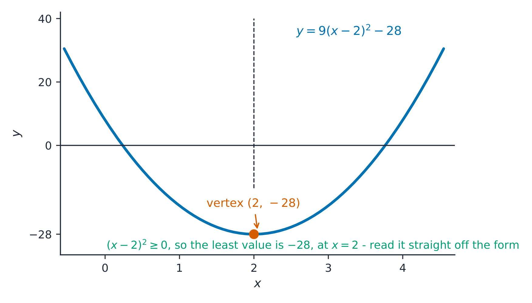
    การเติมกำลังสองช่วยหาจุดยอดของพาราโบลา
    การเติมกำลังสองช่วยหาจุดยอดของพาราโบลา
    • สำหรับ ฟังก์ชันเชิงเส้น อัตราการเปลี่ยนแปลงเฉลี่ยในช่วงใดๆ เป็น ค่าคงที่ – ดังนั้นอัตราที่อัตราเปลี่ยนแปลงเป็นศูนย์
    • สำหรับ ฟังก์ชันกำลังสอง อัตราการเปลี่ยนแปลงเฉลี่ยในช่วงที่มีความยาวเท่ากัน จะสร้างรูปแบบ เชิงเส้น – ดังนั้นอัตรานั้นๆ เปลี่ยนแปลงด้วย อัตราคงที่

    แนวคิด "อัตราของอัตรา" นี้แยกประเภทฟังก์ชัน: ผลต่างระดับที่สองที่คงที่บ่งบอกถึงฟังก์ชันกำลังสอง

    สะพานโกลเด้น เกตพร้อมสายเคเบิลหลักโค้งมน
    สายเคเบิลสะพานแขวนมีรูปร่างคล้ายพาราโบลา – ฟังก์ชันกำลังสองที่เราเห็นได้ในโครงสร้างเหล็ก
    Explore · ⁨สำรวจ⁩

    Explore a quadratic's changing rate · ⁨สำรวจอัตราการเปลี่ยนแปลงของฟังก์ชันกำลังสอง⁩

    y = ax² + bx + c

    Move the sliders and watch the parabola 抛物线 tilt. Its average rate of change is not constant — the slope is positive on one side of the vertex 顶点 and negative on the other. Notice how $a$ opens it up or down. · ⁨เลื่อนสไลเดอร์และดู พาราโบลา 抛物线 บิดตัว อัตราการเปลี่ยนแปลงเฉลี่ย ไม่ คงที่ — ความชันเป็นบวกด้านหนึ่งของ ยอด 顶点 และเป็นลบอีกด้าน ระวังว่า $a$ เปิดขึ้นหรือลงอย่างไร⁩

    1.4

    Polynomial Functions and Rates of Change · ⁨ฟังก์ชันพหุนามและอัตราการเปลี่ยนแปลง⁩

    Syllabus · ⁨หลักสูตร⁩
    English

    Learning Objective 1.4.A: Identify key characteristics of polynomial functions related to rates of change.

    • 1.4.A.1 A nonconstant polynomial function of $x$ is any function representation that is equivalent to the analytical form $p(x) = a_n x^n + a_{n-1} x^{n-1} + a_{n-2} x^{n-2} + \ldots + a_2 x^2 + a_1 x + a_0$, where $n$ is a positive integer, $a_i$ is a real number for each $i$ from $1$ to $n$, and $a_n$ is nonzero. The polynomial has degree $n$, the leading term is $a_n x^n$, and the leading coefficient is $a_n$. A constant is also a polynomial function of degree zero.
    • 1.4.A.2 Where a polynomial function switches between increasing and decreasing, or at the included endpoint of a polynomial with a restricted domain, the polynomial function will have a local, or relative, maximum or minimum output value. Of all local maxima, the greatest is called the global, or absolute, maximum. Likewise, the least of all local minima is called the global, or absolute, minimum.
    • 1.4.A.3 Between every two distinct real zeros of a nonconstant polynomial function, there must be at least one input value corresponding to a local maximum or local minimum.
    • 1.4.A.4 Polynomial functions of an even degree will have either a global maximum or a global minimum.
    • 1.4.A.5 Points of inflection of a polynomial function occur at input values where the rate of change of the function changes from increasing to decreasing or from decreasing to increasing. This occurs where the graph of a polynomial function changes from concave up to concave down or from concave down to concave up.
    ไทย

    จุดประสงค์การเรียนรู้ 1.4.A: ระบุลักษณะสำคัญของฟังก์ชันพหุนามที่เกี่ยวข้องกับอัตราการเปลี่ยนแปลง

    • 1.4.A.1 ฟังก์ชันพหุนามที่ไม่เป็นค่าคงที่ $x$ คือ任何形式的ที่เทียบเท่ากับรูปแบบวิเคราะห์ $p(x) = a_n x^n + a_{n-1} x^{n-1} + a_{n-2} x^{n-2} + \ldots + a_2 x^2 + a_1 x + a_0$ โดยที่ $n$ เป็นจำนวนเต็มบวก $a_i$ เป็นจำนวนจริงสำหรับแต่ละ $i$ ตั้งแต่ $1$ ถึง $n$ และ $a_n$ ไม่เป็นศูนย์ พหุนามมีดีกรี $n$ พจน์นำคือ $a_n x^n$ และสัมประสิทธิ์นำคือ $a_n$ ค่าคงที่ก็เป็นฟังก์ชันพหุนามดีกรีศูนย์ได้เช่นกัน
    • 1.4.A.2 ที่ตำแหน่งที่ฟังก์ชันพหุนามเปลี่ยนจากเพิ่มเป็นลด หรือที่ขอบเขตของโดเมนที่จำกัด ฟังก์ชันพหุนามจะมีค่า output สูงสุดหรือต่ำสุด เฉพาะจุด (local หรือ relative) จากสูงสุดเฉพาะจุดทั้งหมด ค่าที่ใหญ่ที่สุดเรียกว่า สูงสุด整个世界 (global หรือ absolute) ในทำนองเดียวกัน ค่าต่ำสุดเฉพาะจุดที่น้อยที่สุดเรียกว่า ต่ำสุด整个世界 (global หรือ absolute)
    • 1.4.A.3 ระหว่างรากจริงที่แตกต่างกันทุกคู่ของฟังก์ชันพหุนามที่ไม่เป็นค่าคงที่ จะต้องมียอดอินพุตอย่างน้อยหนึ่งค่าที่สอดคล้องกับค่าสูงสุดเฉพาะจุดหรือค่าต่ำสุดเฉพาะจุด
    • 1.4.A.4 ฟังก์ชันพหุนามดีกรีคู่จะมีทั้งสูงสุด整个世界หรือต่ำสุด整个世界อย่างใดอย่างหนึ่ง
    • 1.4.A.5 จุดเปลี่ยนความโค้ง ของฟังก์ชันพหุนามเกิดขึ้นที่ค่าอินพุตที่อัตราการเปลี่ยนแปลงของฟังก์ชันเปลี่ยนจากเพิ่มขึ้นเป็นลดลงหรือจากลดลงเป็นเพิ่มขึ้น สิ่งนี้เกิดขึ้นเมื่อกราฟของฟังก์ชันพหุนามเปลี่ยนจากความโค้งขึ้นเป็นความโค้งลงหรือจากความโค้งลงเป็นความโค้งขึ้น

    Source: College Board AP Course and Exam Description · ⁨แหล่งที่มา: คำอธิบายหลักสูตรและข้อสอบ College Board AP⁩

    English

    A nonconstant polynomial 多项式 has the form

    $$p(x)=a_n x^n + a_{n-1}x^{n-1}+\cdots+a_1 x + a_0,\quad a_n\neq 0.$$
    Its degree 次数 is $n$, its leading term 首项 is $a_n x^n$, and its leading coefficient 首项系数 is $a_n$. A constant is a polynomial of degree $0$.

    Key features:

    • Where a polynomial switches between increasing and decreasing, it has a local (relative) extremum 局部极值. The greatest local maximum is the global (absolute) maximum 全局最大值 only when the polynomial has one — but most polynomials are unbounded (every odd-degree polynomial runs off to $\pm\infty$), so they have no global maximum or minimum at all.
    • Between any two distinct real zeros there is at least one local maximum or minimum.
    • An even-degree polynomial has either a global maximum or a global minimum.
    • A point of inflection 拐点 is where the graph changes concavity – from concave up 上凹 to concave down 下凹 or the reverse – i.e. where the rate of change switches between increasing and decreasing.
    • A function has symmetry when it is even 偶函数 – $f(-x)=f(x)$, graph symmetric across the $y$-axis (like $x^2$, $x^4$) – or odd 奇函数 – $f(-x)=-f(x)$, graph symmetric by rotation about the origin (like $x^3$, $x^5$). Test by substituting $-x$ and simplifying; later, $\cos\theta$ is even and $\sin\theta$ is odd.
    ไทย
    เส้นโค้งสะพานที่ลื่นไหล: กราฟพหุนามและฟังก์ชันตรรกยะจำลองรูปทรงจริงพร้อมเส้น asimptote และจุดเปลี่ยนทิศทาง
    เส้นโค้งสะพานที่ลื่นไหล: กราฟพหุนามและฟังก์ชันตรรกยะจำลองรูปทรงจริงพร้อมเส้น asimptote และจุดเปลี่ยนทิศทาง

    พหุนามที่ไม่ใช่ค่าคงที่ มีรูปแบบเป็น

    $$p(x)=a_n x^n + a_{n-1}x^{n-1}+\cdots+a_1 x + a_0,\quad a_n\neq 0.$$
    ดีกรี ของมันคือ $n$, พจน์นำหน้า คือ $a_n x^n$, และ สัมประสิทธิ์นำหน้า คือ $a_n$ ค่าคงที่คือพหุนามที่มีดีกรี $0$.

    คุณสมบัติสำคัญ:

    • ที่ที่พหุนามสลับระหว่างเพิ่มและลด จะมี จุดสูงสุดหรือต่ำสุดเฉพาะ局部 (local/relative extremum) ค่าสูงสุดเฉพาะ局部ที่ใหญ่ที่สุดคือ ค่าสูงสุดสัมบูรณ์ (global/absolute maximum) ก็ต่อเมื่อพหุนามมีแค่จุดเดียว – แต่พหุนามส่วนใหญ่ไม่มีขอบเขต (พหุนามดีกรีคี่จะพุ่งออกไปยัง $\pm\infty$), ดังนั้นจึงไม่มีค่าสูงสุดหรือต่ำสุดสัมบูรณ์เลย
    • ระหว่างรากจริงที่แตกต่างกันสองจุด จะมีจุดสูงสุดหรือต่ำสุดเฉพาะ局部อย่างน้อยหนึ่งจุด
    • พหุนาม ดีกรีคู่ จะมีค่าสูงสุดหรือค่าต่ำสุดสัมบูรณ์อย่างใดอย่างหนึ่ง
    • จุดเปลี่ยนเว้า (point of inflection) คือจุดที่กราฟเปลี่ยนความเว้า – จาก เว้าขึ้น (concave up) เป็น เว้าลง (concave down) หรือในทางกลับกัน – นั่นคือจุดที่อัตราการเปลี่ยนแปลงสลับระหว่างเพิ่มและลด
    • ฟังก์ชันมี ความสมมาตร เมื่อเป็น ฟังก์ชันคู่ (even) – $f(-x)=f(x)$, กราฟสมมาตรผ่านแกน $y$ (เช่น $x^2$, $x^4$) – หรือ ฟังก์ชันคี่ (odd) – $f(-x)=-f(x)$, กราฟสมมาตรด้วยการหมุนรอบจุดกำเนิด (เช่น $x^3$, $x^5$). ตรวจสอบโดยการแทนค่า $-x$ และจัดรูป; ในภายหลัง $\cos\theta$ เป็นฟังก์ชันคู่และ $\sin\theta$ เป็นฟังก์ชันคี่
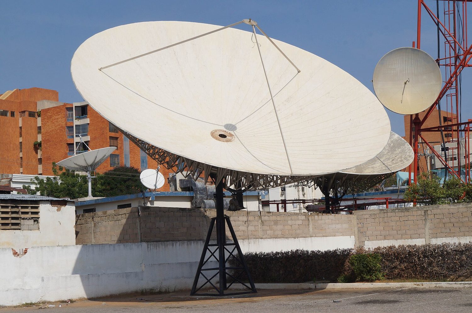
    จานดาวเทียมติดตั้งบนผนัง dengan reflektorโค้งชี้ฟ้า โดยมีตัวรับสัญญาณอยู่ที่โฟกัส
    จานดาวเทียมคือพาราโบลาหมุน: รังสีขนานทุกเส้นสะท้อนไปยังโฟกัสเดียวกัน
    Vocabulary · ⁨คำศัพท์⁩ Train · ⁨ฝึกฝน⁩
    English ไทย
    function/ˈfʌŋkʃn/ function
    domain/dəˈmeɪn/ โดเมน
    range/reɪndʒ/ range
    independent variable/ˌɪndɪˈpendənt ˈveərɪəbl/ ตัวแปรอิสระ
    dependent variable/dɪˈpendənt ˈveərɪəbl/ ตัวแปรตาม
    increasing/ɪnˈkriːsɪŋ/ เพิ่มขึ้น
    decreasing/ˈdiːkriːsɪŋ/ ลดลง
    average rate of change/ˈævrɪdʒ reɪt ɒv tʃeɪndʒ/ อัตราการเปลี่ยนแปลงเฉลี่ย
    secant line/ˈsiːkənt laɪn/ เส้น sécant
    linear/ˈlɪnɪə/ linear
    quadratic/kwɒˈdrætɪk/ พหุนามกำลังสอง
    polynomial/ˌpɒlɪˈnəʊmɪəl/ พหุนาม
    degree/dɪˈɡriː/ ดีกรี
    leading term/ˈliːdɪŋ tɜːm/ พจน์นำ
    leading coefficient/ˈliːdɪŋ ˌkəʊɪˈfɪʃənt/ สัมประสิทธิ์นำ
    local (relative) extremum/ˈləʊkl ekˈstreməm/ จุดสุดขั้วในท้องถิ่น (สัมพัทธ์)
    global (absolute) maximum/ˈɡləʊbl ˈmæksɪməm/ ค่าสูงสุด global (absolute) maximum
    point of inflection/pɔɪnt ɒv ɪnˈflekʃn/ จุดเปลี่ยนเว้า
    concave up/kɒnˈkeɪv ʌp/ เว้าขึ้น
    concave down/kɒnˈkeɪv daʊn/ โค้งลง
    even/ˈiːvən/ even
    odd/ɒd/ จำนวนคี่
    zero/ˈzɪərəʊ/ ศูนย์
    root/ruːt/ ราก
    1.5

    Polynomial Functions and Complex Zeros · ⁨ฟังก์ชันพหุนามและรากซับซ้อน⁩

    Syllabus · ⁨หลักสูตร⁩
    English

    Learning Objective 1.5.A: Identify key characteristics of a polynomial function related to its zeros when suitable factorizations are available or with technology.

    • 1.5.A.1 If $a$ is a complex number and $p(a) = 0$, then $a$ is called a zero of the polynomial function $p$, or a root of $p(x) = 0$. If $a$ is a real number, then $(x - a)$ is a linear factor of $p$ if and only if $a$ is a zero of $p$.
    • 1.5.A.2 If a linear factor $(x - a)$ is repeated $n$ times, the corresponding zero of the polynomial function has a multiplicity $n$. A polynomial function of degree $n$ has exactly $n$ complex zeros when counting multiplicities.
    • 1.5.A.3 If $a$ is a real zero of a polynomial function $p$, then the graph of $y = p(x)$ has an $x$-intercept at the point $(a, 0)$. Consequently, real zeros of a polynomial can be endpoints for intervals satisfying polynomial inequalities.
    • 1.5.A.4 If $a + bi$ is a non-real zero of a polynomial function $p$, then its conjugate $a - bi$ is also a zero of $p$.
    • 1.5.A.5 If the real zero, $a$, of a polynomial function has even multiplicity, then the signs of the output values are the same for input values near $x = a$. For these polynomial functions, the graph will be tangent to the $x$-axis at $x = a$.
    • 1.5.A.6 The degree of a polynomial function can be found by examining the successive differences of the output values over equal-interval input values. The degree of the polynomial function is equal to the least value $n$ for which the successive $n$th differences are constant.

    Learning Objective 1.5.B: Determine if a polynomial function is even or odd.

    • 1.5.B.1 An even function is graphically symmetric over the line $x = 0$ and analytically has the property $f(-x) = f(x)$. If $n$ is even, then a polynomial of the form $p(x) = a_n x^n$, where $n \geq 1$ and $a_n \neq 0$, is an even function.
    • 1.5.B.2 An odd function is graphically symmetric about the point $(0, 0)$ and analytically has the property $f(-x) = -f(x)$. If $n$ is odd, then a polynomial of the form $p(x) = a_n x^n$, where $n \geq 1$ and $a_n \neq 0$, is an odd function.
    ไทย

    จุดประสงค์การเรียนรู้ 1.5.A: ระบุลักษณะสำคัญของฟังก์ชันพหุนามที่เกี่ยวข้องกับรากเมื่อมีตัวประกอบที่เหมาะสมหรือใช้เทคโนโลยีช่วย

    • 1.5.A.1 ถ้า $a$ เป็นจำนวนเชิงซ้อนและ $p(a) = 0$ แล้ว $a$ เรียกว่า ราก ของฟังก์ชันพหุนาม $p$ หรือ รากสมการ ของ $p(x) = 0$ ถ้า $a$ เป็นจำนวนจริง แล้ว $(x - a)$ เป็นตัวประกอบเชิงเส้นของ $p$ ก็ต่อเมื่อ $a$ เป็นรากของ $p$
    • 1.5.A.2 หากตัวประกอบเชิงเส้น $(x - a)$ ซ้ำกัน $n$ ครั้ง รากที่เกี่ยวข้องของฟังก์ชันพหุนามจะมี ความซ้ำซ้อน (multiplicity) เท่ากับ $n$ ฟังก์ชันพหุนามที่มี ดีกรี $n$ จะมีรากเชิงซ้อนจำนวน $n$ พอดีเมื่อนับตามความซ้ำซ้อน
    • 1.5.A.3 หาก $a$ เป็นรากจริงของฟังก์ชันพหุนาม $p$ แล้วกราฟของ $y = p(x)$ จะมีจุดตัดแกน $x$ ที่จุด $(a, 0)$ ดังนั้น รากจริงของพหุนามจึงสามารถเป็นจุดปลายของช่วงที่สอดคล้องกับความไม่เท่าเทียมทางพหุนามได้
    • 1.5.A.4 ถ้า $a + bi$ เป็นรากที่ไม่ใช่จำนวนจริงของฟังก์ชันพหุนาม $p$ แล้ว จำนวน-queryate ของมัน $a - bi$ ก็เป็นรากของ $p$ เช่นกัน
    • 1.5.A.5 หากรากจริง $a$ ของฟังก์ชันพหุนามมีความซ้ำซ้อนเป็นเลขคู่แล้ว สัญญาณของค่าเอาต์พุตจะเป็นเหมือนกันสำหรับค่าอินพุตใกล้กับ $x = a$ สำหรับฟังก์ชันพหุนามเหล่านี้ กราฟจะสัมผัสกับ $x$-แกน ที่ $x = a$
    • 1.5.A.6 ดีกรีของฟังก์ชันพหุนามสามารถหาได้โดยการตรวจสอบผลต่างติดต่อกันของค่า output ในช่วงค่าอินพุตที่มีระยะห่างเท่ากัน ดีกรีของฟังก์ชันพหุนามจะเท่ากับค่าน้อยที่สุด $n$ ที่ผลต่างระดับที่ $n$ ติดต่อกันมีค่าคงที่

    จุดประสงค์การเรียนรู้ 1.5.B: กำหนดว่าฟังก์ชันพหุนามเป็นฟังก์ชันคู่หรือฟังก์ชันคี่

    • 1.5.B.1 ฟังก์ชันคู่ มีกราฟสมมาตรเหนือเส้น $x = 0$ และมีคุณสมบัติทางวิเคราะห์ $f(-x) = f(x)$ ถ้า $n$ เป็นคู่ entonces-funcion of the form $p(x) = a_n x^n$ โดยที่ $n \geq 1$ และ $a_n \neq 0$ เป็นฟังก์ชันคู่
    • 1.5.B.2 ฟังก์ชัน คี่ มีสมมาตรรอบจุด $(0, 0)$ บนแผนภูมิ และมีคุณสมบัติทางวิเคราะห์คือ $f(-x) = -f(x)$ หาก $n$ เป็นฟังก์ชันคี่ แล้วพหุนามที่มีรูป $p(x) = a_n x^n$ โดยที่ $n \geq 1$ และ $a_n \neq 0$ เป็นฟังก์ชันคี่

    Source: College Board AP Course and Exam Description · ⁨แหล่งที่มา: คำอธิบายหลักสูตรและข้อสอบ College Board AP⁩

    English

    A zero 零点 (or root 根) of $p$ is a number $a$ with $p(a)=0$. For a real $a$, $(x-a)$ is a factor of $p$ exactly when $a$ is a zero. If the factor $(x-a)$ is repeated $n$ times, that zero has multiplicity 重数 $n$. Counting multiplicities, a degree-$n$ polynomial has exactly $n$ complex 复数 zeros.

    • A real zero $a$ gives an $x$-intercept at $(a,0)$; real zeros are the endpoints of the intervals where $p(x)\ge 0$ or $\le 0$.
    • Non-real zeros come in conjugate 共轭 pairs: if $a+bi$ is a zero, so is $a-bi$.
    • At a real zero of even multiplicity the graph is tangent to the $x$-axis (it touches but does not cross); at odd multiplicity it crosses.
    • The degree equals the least $n$ for which the $n$th successive differences of equally-spaced outputs become constant.
    ไทย

    ศูนย์ (หรือ ราก) ของ $p$ คือจำนวน $a$ ที่มี $p(a)=0$. สำหรับพหุนามจริง $a$, $(x-a)$ เป็นปัจจัยของ $p$ ก็ต่อเมื่อ $a$ เป็นศูนย์. ถ้าปัจจัย $(x-a)$ ซ้ำกัน $n$ ครั้ง, ศูนย์นี้มี ดีกรี (multiplicity) เท่ากับ $n$. เมื่อนับดีกรีแล้ว พหุนามดีกรี $n$ จะมีศูนย์ เชิงซ้อน จำนวน $n$ ตัวพอดี

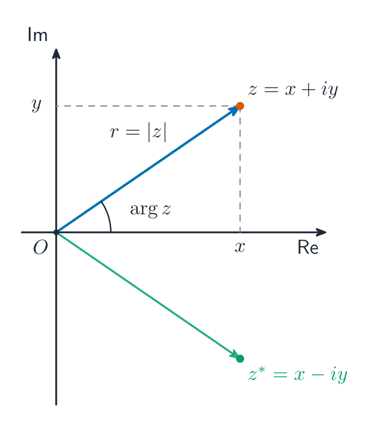
    จำนวนซ้อนบนแผนภาพอาร์แอกันด: โมดูลัสคือระยะทาง, อาร์กิวเมนต์คือมุม
    จำนวนซ้อนบนแผนภาพอาร์แอกันด: โมดูลัสคือระยะทาง, อาร์กิวเมนต์คือมุม
    • รากจริง $a$ จะให้ $x$-intercept ที่ $(a,0)$; รากจริงคือจุดปลายของช่วงที่ $p(x)\ge 0$ หรือ $\le 0$.
    • รากไม่จริงมาในรูปแบบ คู่สังยุค (conjugate pairs): ถ้า $a+bi$ เป็นราก那么 $a-bi$ ก็เป็นรากเช่นกัน
    • ที่รากจริงที่มี even multiplicity กราฟจะเป็น tangent กับ $x$-axis (สัมผัสแต่ไม่ตัด); สำหรับ odd multiplicity มันจะตัด
    • ดีกรีเท่ากับค่าต่ำสุดของ $n$ ที่ผลต่าง $n$次 (successive differences) ของผลลัพธ์ที่มีระยะห่างเท่ากันเป็นค่าคงที่
    Vocabulary · ⁨คำศัพท์⁩ Train · ⁨ฝึกฝน⁩
    English ไทย
    multiplicity/ˌmʌltɪˈplɪsɪti/ ความซ้ำซ้อน
    complex/ˈkɒmpleks/ ซับซ้อน
    conjugate/ˈkɒndʒuːɡeɪt/ คอนจูเกต
    1.6

    Polynomial Functions and End Behavior · ⁨ฟังก์ชันพหุนามและพฤติกรรมที่ปลาย⁩

    Syllabus · ⁨หลักสูตร⁩
    Learning ObjectiveEssential Knowledge

    1.6.A
    Describe end behaviors of polynomial functions.

    • 1.6.A.1 As input values of a nonconstant polynomial function increase without bound, the output values will either increase or decrease without bound. The corresponding mathematical notation is $\lim_{x \to \infty} p(x) = \infty$ or $\lim_{x \to \infty} p(x) = -\infty$.
    • 1.6.A.2 As input values of a nonconstant polynomial function decrease without bound, the output values will either increase or decrease without bound. The corresponding mathematical notation is $\lim_{x \to -\infty} p(x) = \infty$ or $\lim_{x \to -\infty} p(x) = -\infty$.
    • 1.6.A.3 The degree and sign of the leading term of a polynomial determines the end behavior of the polynomial function, because as the input values increase or decrease without bound, the values of the leading term dominate the values of all lower-degree terms.

    Source: College Board AP Course and Exam Description · ⁨แหล่งที่มา: คำอธิบายหลักสูตรและข้อสอบ College Board AP⁩

    English

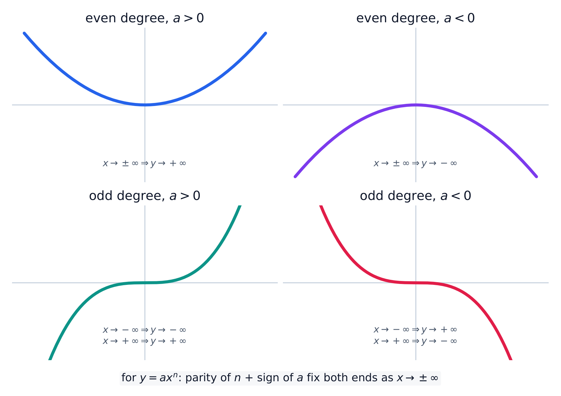
    End behavior 末端行为 describes where a function heads as the input grows without bound. For a nonconstant polynomial, as $x\to\pm\infty$ the output goes to $+\infty$ or $-\infty$, written e.g. $\lim_{x\to\infty}p(x)=\infty$. Which way depends entirely on the leading term $a_n x^n$, because for large $|x|$ it dominates all lower-degree terms: the sign of $a_n$ and whether $n$ is even or odd fix both ends.

    ไทย

    พฤติกรรมที่ปลาย (end behavior) อธิบายว่าฟังก์ชัน去向何方เมื่ออินพุตมีค่ามากขึ้นอย่างไม่จำกัด สำหรับพหุนามที่ไม่ใช่ค่าคงที่ เมื่อ $x\to\pm\infty$ เอาต์พุตจะgoing to $+\infty$ หรือ $-\infty$, เขียนเช่น $\lim_{x\to\infty}p(x)=\infty$. ทิศทางขึ้นอยู่กับ พจน์นำหน้า $a_n x^n$ เท่านั้น เพราะสำหรับ $|x|$ ใหญ่ๆ มัน ครอบงำ พจน์ดีกรีต่ำกว่าทั้งหมด: สัญญาณของ $a_n$ และการที่ $n$ เป็นคู่หรือคี่กำหนดทั้งสองปลาย

    ปลายของพหุนามทุกตัวถูกกำหนดโดยความคู่-คี่ของดีกรีและเครื่องหมายของสัมประสิทธิ์หน้าสุด
    ปลายของพหุนามทุกตัวถูกกำหนดโดยความคู่-คี่ของดีกรีและเครื่องหมายของสัมประสิทธิ์หน้าสุด
    Explore · ⁨สำรวจ⁩

    See how the leading term sets the end behavior · ⁨เห็นได้ว่าพจน์แรกกำหนดพฤติกรรมขอบเขต⁩

    y = ax³ + bx² + cx + d

    The leading term decides the ends. For a cubic with $a>0$ the graph falls on the left and rises on the right; make $a<0$ and the two ends swap. As $x\to\pm\infty$ the highest-power term dominates every other term. · ⁨พจน์แรก กำหนดปลายกราฟ สำหรับฟังก์ชันลูกบาศก์ที่มี $a>0$ กราฟจะลดลงทางซ้ายและเพิ่มขึ้นทางขวา; ทำให้ $a<0$ และปลายทั้งสองสลับกัน เมื่อ $x\to\pm\infty$ พจน์กำลังสูงสุดจะครอบงำทุกพจน์อื่น⁩

    Vocabulary · ⁨คำศัพท์⁩ Train · ⁨ฝึกฝน⁩
    English ไทย
    End behavior/end bɪˈheɪvjə/ พฤติกรรมที่ปลาย
    rational function/ˈræʃənl ˈfʌŋkʃn/ ฟังก์ชันตรรกยะ
    slant asymptote/slænt ˈæsɪmptəʊt/ เส้นแนวนอนเฉียง
    horizontal asymptote/ˌhɒrɪˈzɒntl ˈæsɪmptəʊt/ เส้นประแนวนอน
    vertical asymptote/ˈvɜːtɪkl ˈæsɪmptəʊt/ เส้นประแนวตั้ง
    hole/həʊl/ จุดว่าง
    Polynomial long division/ˌpɒlɪˈnəʊmɪəl lɒŋ dɪˈvɪʒn/ การหารพหุนามยาว
    quotient/ˈkwəʊʃənt/ ผลหาร
    remainder/rɪˈmeɪndə/ เศษ
    1.7

    Rational Functions and End Behavior · ⁨ฟังก์ชันตรรกยะและการ davranที่ปลาย⁩

    Syllabus · ⁨หลักสูตร⁩
    English

    Learning Objective 1.7.A: Describe end behaviors of rational functions.

    • 1.7.A.1 A rational function is analytically represented as a quotient of two polynomial functions and gives a measure of the relative size of the polynomial function in the numerator compared to the polynomial function in the denominator for each value in the rational function's domain.
    • 1.7.A.2 The end behavior of a rational function will be affected most by the polynomial with the greater degree, as its values will dominate the values of the rational function for input values of large magnitude. For input values of large magnitude, a polynomial is dominated by its leading term. Therefore, the end behavior of a rational function can be understood by examining the corresponding quotient of the leading terms.
    • 1.7.A.3 If the polynomial in the numerator dominates the polynomial in the denominator for input values of large magnitude, then the quotient of the leading terms is a nonconstant polynomial, and the original rational function has the end behavior of that polynomial. If that polynomial is linear, then the graph of the rational function has a slant asymptote parallel to the graph of the line.
    • 1.7.A.4 If neither polynomial in a rational function dominates the other for input values of large magnitude, then the quotient of the leading terms is a constant, and that constant indicates the location of a horizontal asymptote of the graph of the original rational function.
    • 1.7.A.5 If the polynomial in the denominator dominates the polynomial in the numerator for input values of large magnitude, then the quotient of the leading terms is a rational function with a constant in the numerator and nonconstant polynomial in the denominator, and the graph of the original rational function has a horizontal asymptote at $y = 0$.
    • 1.7.A.6 When the graph of a rational function $r$ has a horizontal asymptote at $y = b$, where $b$ is a constant, the output values of the rational function get arbitrarily close to $b$ and stay arbitrarily close to $b$ as input values increase or decrease without bound. The corresponding mathematical notation is $\lim_{x \to \infty} r(x) = b$ or $\lim_{x \to -\infty} r(x) = b$.
    ไทย

    จุดประสงค์การเรียนรู้ 1.7.A: อธิบายพฤติกรรมที่ขอบเขตของฟังก์ชันตรรกยะ

    • 1.7.A.1 ฟังก์ชันตรรกยะถูกแสดงในรูปแบบวิเคราะห์เป็นผลหารของฟังก์ชันพหุนามสองตัว และเป็นการวัดขนาดสัมพัทธ์ของฟังก์ชันพหุนามในตัวเศษเทียบกับฟังก์ชันพหุนามในตัวส่วนสำหรับแต่ละค่าในโดเมนของฟังก์ชันตรรกยะ
    • 1.7.A.2 พฤติกรรมปลายของฟังก์ชันพหุนามส่วนจะได้รับผลกระทบมากที่สุดจากพหุนามที่มีดีกรีสูงกว่า เนื่องจากค่าของมันจะครอบงำค่าของฟังก์ชันพหุนามส่วนสำหรับค่าอินพุตที่มีขนาดมาก สำหรับค่าอินพุตที่มีขนาดมาก พหุนามจะถูกครอบงำโดยเทอมแรก ดังนั้น พฤติกรรมปลายของฟังก์ชันพหุนามส่วนจึงสามารถเข้าใจได้โดยการพิจารณาผลหารของเทอมแรกที่เกี่ยวข้อง
    • 1.7.A.3 หากพหุนามในตัวเศษครอบงำพหุนามในตัวส่วนสำหรับค่าอินพุตที่มีขนาดมาก ผลหารของเทอมแรกจะเป็นพหุนามที่ไม่ใช่ค่าคงที่ และฟังก์ชันพหุนามส่วนเดิมจะมีพฤติกรรมปลายตามพหุนามนั้น หากพหุนามนี้เป็นเชิงเส้น กราฟของฟังก์ชันพหุนามส่วนจะมีเส้นประเฉียงขนานกับกราฟของเส้นตรงนั้น
    • 1.7.A.4 หากไม่มีพหุนามใดในฟังก์ชันพหุนามส่วนครอบงำอีกฝ่ายสำหรับค่าอินพุตที่มีขนาดมาก ผลหารของเทอมแรกจะเป็นค่าคงที่ และค่าคงที่นั้นบ่งบอกตำแหน่งของเส้นประแนวนอนของกราฟฟังก์ชันพหุนามส่วนเดิม
    • 1.7.A.5 หากพหุนามในตัวส่วนครอบงำพหุนามในตัวเศษสำหรับค่าอินพุตที่มีขนาดมาก ผลหารของเทอมแรกจะเป็นฟังก์ชันพหุนามส่วนที่มีค่าคงที่ในตัวเศษและพหุนามที่ไม่ใช่ค่าคงที่ในตัวส่วน และกราฟของฟังก์ชันพหุนามส่วนเดิมจะมีเส้นประแนวนอนที่ $y = 0$
    • 1.7.A.6 เมื่อกราฟของฟังก์ชันพหุนามส่วน $r$ มีเส้นประแนวนอนที่ $y = b$ โดยที่ $b$ เป็นค่าคงที่ ค่าเอาต์พุตของฟังก์ชันพหุนามส่วนจะเข้าใกล้ $b$ อย่างใกล้ชิดเท่าที่จะเป็นไปได้และยังคงอยู่ใกล้ $b$ อย่างใกล้ชิดเท่าที่จะเป็นไปเมื่อค่าอินพุตเพิ่มขึ้นหรือลดลงโดยไม่จำกัด ขีดเขตทางคณิตศาสตร์ที่เกี่ยวข้องคือ $\lim_{x \to \infty} r(x) = b$ หรือ $\lim_{x \to -\infty} r(x) = b$

    Source: College Board AP Course and Exam Description · ⁨แหล่งที่มา: คำอธิบายหลักสูตรและข้อสอบ College Board AP⁩

    English

    A rational function 有理函数 is a quotient of two polynomials, $r(x)=\dfrac{\text{numerator}}{\text{denominator}}$. Its end behavior is governed by the quotient of the leading terms:

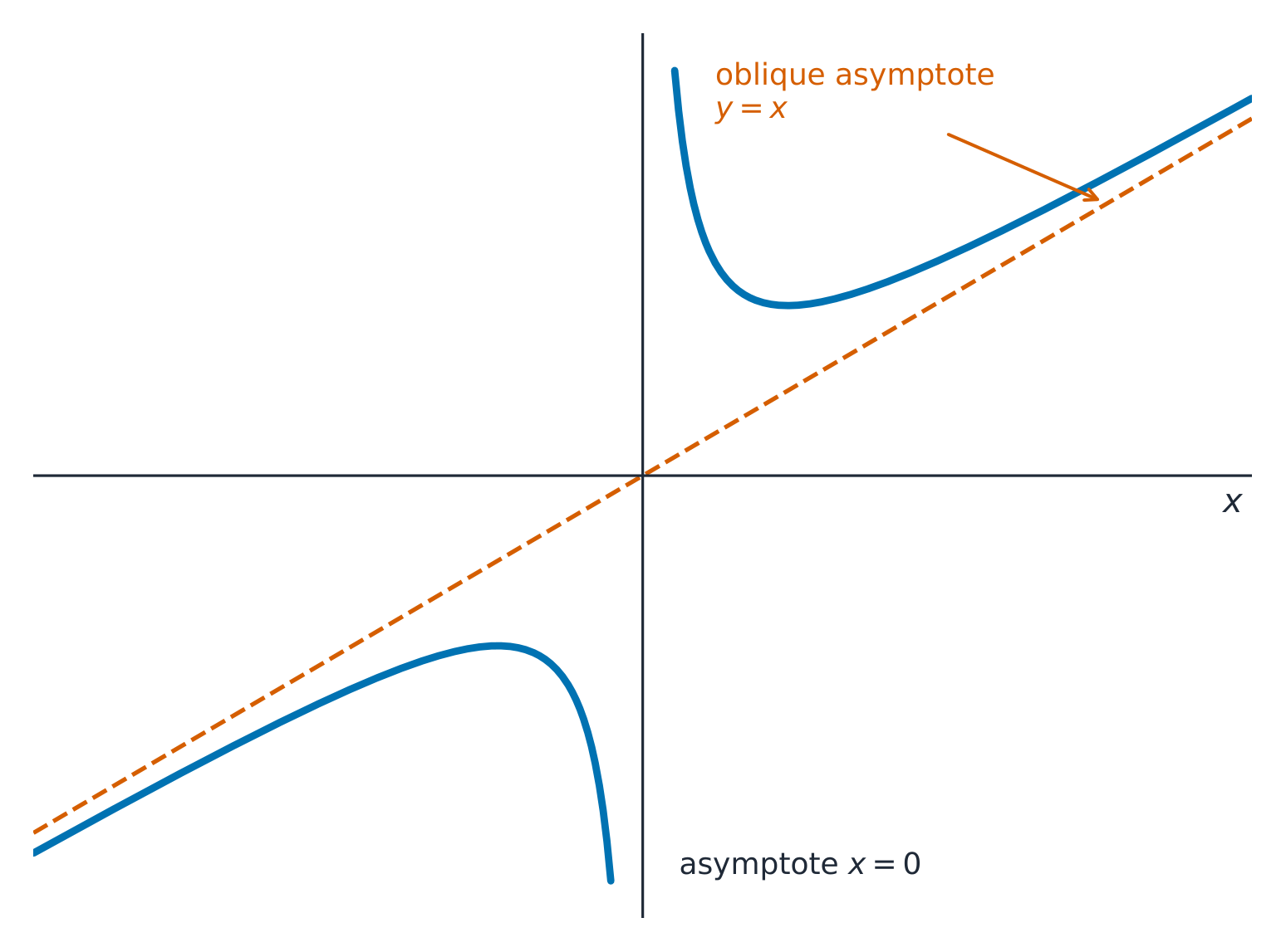
    • Numerator degree > denominator degree: the quotient is a nonconstant polynomial, and $r$ follows that polynomial's end behavior. If that quotient is linear, the graph has a slant asymptote 斜渐近线.
    • Equal degrees: the quotient is a constant, giving a horizontal asymptote 水平渐近线 $y=$ the ratio of leading coefficients.
    • Numerator degree < denominator degree: the quotient tends to $0$, so the horizontal asymptote is $y=0$.

    At a horizontal asymptote $y=b$, the outputs get and stay arbitrarily close to $b$: $\lim_{x\to\pm\infty}r(x)=b$.

    ไทย

    ฟังก์ชันตรรกยะ คือเศษส่วนของพหุนามสองตัว, $r(x)=\dfrac{\text{numerator}}{\text{denominator}}$. พฤติกรรมปลายทางถูกกำหนดโดย ผลหารของพจน์นำ:

    เมื่อตัวเศษมีดีกรีสูงกว่า กราฟจะเข้าใกล้เส้นอสมการเฉียง
    เมื่อตัวเศษมีดีกรีสูงกว่า กราฟจะเข้าใกล้เส้นอสมการเฉียง
    • ดีกรีของตัวเศษ > ดีกรีของตัวส่วน: ผลหารจะเป็นพหุนามที่ไม่ใช่ค่าคงที่, และ $r$ จะแสดงพฤติกรรมที่ปลายตามพหุนามนั้น หากผลหารนี้เป็นเชิงตรง กราฟจะมี เส้นอสมการเฉียง.
    • ดีกรีเท่ากัน: ผลหารจะเป็นค่าคงที่, ซึ่งให้ เส้นอสมการแนวนอน $y=$ คืออัตราส่วนของสัมประสิทธิ์หน้าสุด.
    • ดีกรีของตัวเศษ < ดีกรีของตัวส่วน: ผลหารจะเข้าหา $0$, ดังนั้นเส้นอสมการแนวนอนคือ $y=0$.

    ที่เส้นแนวนอน $y=b$, ค่าผลลัพธ์จะเข้าใกล้และคงอยู่ใกล้เคียงกับ $b$ อย่างอิสระ: $\lim_{x\to\pm\infty}r(x)=b$.

    1.8

    Rational Functions and Zeros · ⁨ฟังก์ชันตรรกยะและจุดศูนย์⁩

    Syllabus · ⁨หลักสูตร⁩
    English

    Learning Objective 1.8.A: Determine the zeros of rational functions.

    • 1.8.A.1 The real zeros of a rational function correspond to the real zeros of the numerator for such values in its domain.
    • 1.8.A.2 The real zeros of both polynomial functions of a rational function $r$ are endpoints or asymptotes for intervals satisfying the rational function inequalities $r(x) \geq 0$ or $r(x) \leq 0$.
    ไทย

    วัตถุประสงค์การเรียนรู้ 1.8.A: หาจุดศูนย์ของฟังก์ชันพหุนามส่วน

    • 1.8.A.1 จุดศูนย์จริงของฟังก์ชันพหุนามส่วนสอดคล้องกับจุดศูนย์จริงของตัวเศษสำหรับค่าที่อยู่ในโดเมนของมัน
    • 1.8.A.2 จุดศูนย์จริงของทั้งสองฟังก์ชันพหุนามของฟังก์ชันพหุนามส่วน $r$ เป็นจุดขอบเขตหรือเส้นประสำหรับช่วงที่อสมการฟังก์ชันพหุนามส่วน $r(x) \geq 0$ หรือ $r(x) \leq 0$ เป็นจริง

    Source: College Board AP Course and Exam Description · ⁨แหล่งที่มา: คำอธิบายหลักสูตรและข้อสอบ College Board AP⁩

    English

    The real zeros of a rational function are the real zeros of its numerator that are still in the domain. These zeros, together with the zeros of the denominator, split the number line into the intervals you test when solving inequalities $r(x)\ge 0$ or $r(x)\le 0$.

    ไทย

    จุดศูนย์จริง ของฟังก์ชันตรรกยะคือจุดศูนย์จริงของ ตัวเศษ ที่ยังคงอยู่ในโดเมน จุดศูนย์เหล่านี้ ร่วมกับจุดศูนย์ของตัวส่วน จะแบ่งจำนวนจริงออกเป็นช่วงที่คุณต้องทดสอบในการแก้อสมการ $r(x)\ge 0$ หรือ $r(x)\le 0$

    1.9

    Rational Functions and Vertical Asymptotes · ⁨ฟังก์ชันตรรกยะและเส้นอสมการแนวตั้ง⁩

    Syllabus · ⁨หลักสูตร⁩
    English

    Learning Objective 1.9.A: Determine vertical asymptotes of graphs of rational functions.

    • 1.9.A.1 If the value $a$ is a real zero of the polynomial function in the denominator of a rational function and is not also a real zero of the polynomial function in the numerator, then the graph of the rational function has a vertical asymptote at $x = a$. Furthermore, a vertical asymptote also occurs at $x = a$ if the multiplicity of $a$ as a real zero in the denominator is greater than its multiplicity as a real zero in the numerator.
    • 1.9.A.2 Near a vertical asymptote, $x = a$, of a rational function, the values of the polynomial function in the denominator are arbitrarily close to zero, so the values of the rational function $r$ increase or decrease without bound. The corresponding mathematical notation is $\lim_{x \to a^+} r(x) = \infty$ or $\lim_{x \to a^+} r(x) = -\infty$ for input values near $a$ and greater than $a$, and $\lim_{x \to a^-} r(x) = \infty$ or $\lim_{x \to a^-} r(x) = -\infty$ for input values near $a$ and less than $a$.
    ไทย

    วัตถุประสงค์การเรียนรู้ 1.9.A: หาเส้นประแนวตั้งของกราฟฟังก์ชันพหุนามส่วน

    • 1.9.A.1 หากค่า $a$ เป็นจุดศูนย์จริงของฟังก์ชันพหุนามในตัวส่วนของฟังก์ชันพหุนามส่วนและไม่เป็นจุดศูนย์จริงของฟังก์ชันพหุนามในตัวเศษด้วย กราฟของฟังก์ชันพหุนามส่วนจะมีเส้นประแนวตั้งที่ $x = a$ นอกจากนี้ เส้นประแนวตั้งยังเกิดขึ้นที่ $x = a$ หากความซ้ำซ้อนของ $a$ ในฐานะจุดศูนย์จริงในตัวส่วนมากกว่าความซ้ำซ้อนในฐานะจุดศูนย์จริงในตัวเศษ
    • 1.9.A.2 ใกล้กับเส้นประแนวตั้ง $x = a$ ของฟังก์ชันพหุนามส่วน ค่าของฟังก์ชันพหุนามในตัวส่วนจะเข้าใกล้ศูนย์อย่างใกล้ชิดเท่าที่จะเป็นไปได้ ดังนั้น ค่าของฟังก์ชันพหุนามส่วน $r$ จะเพิ่มขึ้นหรือลดลงโดยไม่จำกัด ขีดเขตทางคณิตศาสตร์ที่เกี่ยวข้องคือ $\lim_{x \to a^+} r(x) = \infty$ หรือ $\lim_{x \to a^+} r(x) = -\infty$ สำหรับค่าอินพุตใกล้ $a$ และมากกว่า $a$ และ $\lim_{x \to a^-} r(x) = \infty$ หรือ $\lim_{x \to a^-} r(x) = -\infty$ สำหรับค่าอินพุตใกล้ $a$ และน้อยกว่า $a$

    Source: College Board AP Course and Exam Description · ⁨แหล่งที่มา: คำอธิบายหลักสูตรและข้อสอบ College Board AP⁩

    English

    A vertical asymptote 垂直渐近线 occurs at $x=a$ when $a$ is a zero of the denominator but not cancelled by the numerator – more precisely, when its multiplicity in the denominator exceeds its multiplicity in the numerator. Near it, the denominator is nearly zero, so $r$ shoots to $\pm\infty$: $\lim_{x\to a^{\pm}}r(x)=\pm\infty$. Check each side, since the two sides can go opposite ways.

    Worked example. Describe $r(x)=\dfrac{2x^2+3}{x^2-1}$. The numerator and denominator have equal degree, so the horizontal asymptote is $y=\dfrac{2}{1}=2$. The denominator $x^2-1$ is zero at $x=\pm1$ and neither cancels, so there are vertical asymptotes at $x=1$ and $x=-1$.

    ไทย

    เส้นอสมการแนวตั้ง เกิดขึ้นที่ $x=a$ เมื่อ $a$ เป็นจุดศูนย์ของ ตัวส่วน แต่ไม่ถูกลบด้วยตัวเศษ – โดยเฉพาะอย่างยิ่งคือเมื่อความซ้ำซ้อน (multiplicity) ของมันในตัวส่วนมากกว่าความซ้ำซ้อนในตัวเศษ ใกล้เคียงจุดนั้น ตัวเศษจะเกือบเป็นศูนย์, ดังนั้น $r$ จะพุ่งไปที่ $\pm\infty$: $\lim_{x\to a^{\pm}}r(x)=\pm\infty$. ตรวจสอบทั้งสองด้าน เนื่องจากทั้งสองด้านอาจไปทางตรงกันข้ามกัน

    ตัวอย่างทำแล้ว. อธิบาย $r(x)=\dfrac{2x^2+3}{x^2-1}$. ตัวเศษและตัวส่วนมี ดีกรีเท่ากัน, ดังนั้นเส้นอสมการแนวนอนคือ $y=\dfrac{2}{1}=2$. ตัวส่วน $x^2-1$ มีค่าเป็นศูนย์ที่ $x=\pm1$ และไม่มีการลบกัน, ดังนั้นจึงมี เส้นอสมการแนวตั้ง ที่ $x=1$ และ $x=-1$.

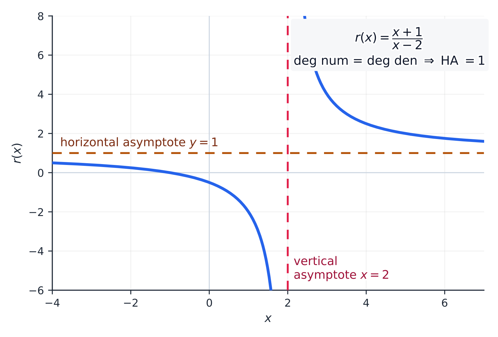
    ฟังก์ชันตรรกยะที่เข้าใกล้เส้นอสมการแนวตั้งและเส้นอสมการแนวนอน
    ฟังก์ชันตรรกยะที่เข้าใกล้เส้นอสมการแนวตั้งและเส้นอสมการแนวนอน
    Explore · ⁨สำรวจ⁩

    Explore a vertical asymptote · ⁨สำรวจเส้น asymptote แนวตั้ง⁩

    y = a/(x − b) + c

    This is $y = \dfrac{a}{x-b} + c$. The graph shoots off toward $\pm\infty$ at the vertical asymptote 竖直渐近线 $x = b$ (where the bottom is zero) and levels off toward the horizontal asymptote 水平渐近线 $y = c$. Slide $b$ and $c$ to move each line. · ⁨นี่คือ $y = \dfrac{a}{x-b} + c$ กราฟพุ่งขึ้นไปหา $\pm\infty$ ที่ เส้น asymptote แนวตั้ง 竖直渐近线 $x = b$ (ที่ส่วนล่างเป็นศูนย์) และราบเรียบเข้าหา เส้น asymptote แนวนอน 水平渐近线 $y = c$ เลื่อน $b$ และ $c$ เพื่อเคลื่อนย้ายแต่ละเส้น⁩

    1.10

    Rational Functions and Holes · ⁨ฟังก์ชันตรรกยะและรูพรุน⁩

    Syllabus · ⁨หลักสูตร⁩
    English

    Learning Objective 1.10.A: Determine holes in graphs of rational functions.

    • 1.10.A.1 If the multiplicity of a real zero in the numerator is greater than or equal to its multiplicity in the denominator, then the graph of the rational function has a hole at the corresponding input value.
    • 1.10.A.2 If the graph of a rational function $r$ has a hole at $x = c$, then the location of the hole can be determined by examining the output values corresponding to input values sufficiently close to $c$. If input values sufficiently close to $c$ correspond to output values arbitrarily close to $L$, then the hole is located at the point with coordinates $(c, L)$. The corresponding mathematical notation is $\lim_{x \to c} r(x) = L$. It should be noted that $\lim_{x \to c^-} r(x) = \lim_{x \to c^+} r(x) = \lim_{x \to c} r(x) = L$.
    ไทย

    วัตถุประสงค์การเรียนรู้ 1.10.A: หาจุดว่างในกราฟของฟังก์ชันตรรกยะ

    • 1.10.A.1 หากความซ้ำซ้อน (multiplicity) ของรากจริงในตัวเศษมีมากกว่าหรือเท่ากับความซ้ำซ้อนในตัวส่วน แล้วกราฟของฟังก์ชันตรรกยะจะมีจุดว่างที่ค่าอินพุตที่เกี่ยวข้อง
    • 1.10.A.2 หากกราฟของฟังก์ชันตรรกยะ $r$ มีจุดว่างที่ $x = c$ ตำแหน่งของจุดว่างสามารถหาได้โดยการพิจารณาค่าเอาต์พุตที่สอดคล้องกับค่าอินพุตที่ใกล้กับ $c$ มากพอ หากค่าอินพุตที่ใกล้กับ $c$ มากพอ สอดคล้องกับค่าเอาต์พุตที่ใกล้เคียงกับ $L$ ได้ตามใจปรารถนา จุดว่างจะอยู่ที่จุดที่มีพิกัด $(c, L)$ Notation ทางคณิตศาสตร์ที่เกี่ยวข้องคือ $\lim_{x \to c} r(x) = L$ ควรสังเกตว่า $\lim_{x \to c^-} r(x) = \lim_{x \to c^+} r(x) = \lim_{x \to c} r(x) = L$

    Source: College Board AP Course and Exam Description · ⁨แหล่งที่มา: คำอธิบายหลักสูตรและข้อสอบ College Board AP⁩

    English

    A hole 空洞 (removable point) occurs at $x=c$ when a factor cancels – the multiplicity of the zero $c$ in the numerator is at least its multiplicity in the denominator. The graph is missing a single point. Its height is the limit of the simplified function: if inputs near $c$ give outputs near $L$, the hole is at $(c,L)$, and $\lim_{x\to c}r(x)=L$.

    ไทย

    รูพรุน (removable point) เกิดขึ้นที่ $x=c$ เมื่อมีตัวประกอบที่ถูกลบออก – ความซ้ำซ้อนของจุดศูนย์ $c$ ในตัวเศษมีอย่างน้อยเท่ากับความซ้ำซ้อนในตัวส่วน กราฟจะขาดหายไปเพียงจุดเดียว ความสูงของมันคือลิมิตของฟังก์ชันที่ลดรูปแล้ว: ถ้าอินพุตใกล้ $c$ ให้เอาต์พุตใกล้ $L$, รูพรุนจะอยู่ที่ $(c,L)$, และ $\lim_{x\to c}r(x)=L$.

    1.11

    Equivalent Representations of Polynomial and Rational Expressions · ⁨รูปแบบที่เทียบเท่าของการแสดงพหุนามและนิพจน์ตรรกยะ⁩

    Syllabus · ⁨หลักสูตร⁩
    English

    Learning Objective 1.11.A: Rewrite polynomial and rational expressions in equivalent forms.

    • 1.11.A.1 Because the factored form of a polynomial or rational function readily provides information about real zeros, it can reveal information about $x$-intercepts, asymptotes, holes, domain, and range.
    • 1.11.A.2 The standard form of a polynomial or rational function can reveal information about end behaviors of the function.
    • 1.11.A.3 The information extracted from different analytic representations of the same polynomial or rational function can be used to answer questions in context.

    Learning Objective 1.11.B: Determine the quotient of two polynomial functions using long division.

    • 1.11.B.1 Polynomial long division is an algebraic process similar to numerical long division involving a quotient and remainder. If the polynomial $f$ is divided by the polynomial $g$, then $f$ can be rewritten as $f(x) = g(x)q(x) + r(x)$, where $q$ is the quotient, $r$ is the remainder, and the degree of $r$ is less than the degree of $g$.
    • 1.11.B.2 The result of polynomial long division is helpful in finding equations of slant asymptotes for graphs of rational functions.

    Learning Objective 1.11.C: Rewrite the repeated product of binomials using the binomial theorem.

    • 1.11.C.1 The binomial theorem utilizes the entries in a single row of Pascal's Triangle to more easily expand expressions of the form $(a + b)^n$, including polynomial functions of the form $p(x) = (x + c)^n$, where $c$ is a constant.
    ไทย

    วัตถุประสงค์การเรียนรู้ 1.11.A: เขียนรูปพหุนามและนิพจน์ตรรกยะให้อยู่ในรูปแบบที่เทียบเท่ากัน

    • 1.11.A.1 เนื่องจากรูปแบบแยกตัวประกอบของพหุนามหรือฟังก์ชันตรรกยะให้ข้อมูลเกี่ยวกับรากจริงได้ง่าย จึงสามารถเปิดเผยข้อมูลเกี่ยวกับจุดตัดแกน $x$, เส้นประสม, จุดว่าง, โดเมน และเรนจ์ได้
    • 1.11.A.2 รูปแบบมาตรฐานของพหุนามหรือฟังก์ชันตรรกยะสามารถเปิดเผยข้อมูลเกี่ยวกับการเปลี่ยนแปลงที่ปลายกราฟ (end behaviors) ของฟังก์ชันได้
    • 1.11.A.3 ข้อมูลที่ได้จากการวิเคราะห์จากรูปแบบการวิเคราะห์ที่แตกต่างกันของพหุนามหรือฟังก์ชันตรรกยะเดียวกัน สามารถใช้เพื่อตอบคำถามในบริบทได้

    วัตถุประสงค์การเรียนรู้ 1.11.B: หาผลหารของฟังก์ชันพหุนามสองฟังก์ชันโดยใช้วิธีหารยาว

    • 1.11.B.1 การหารยาวของพหุนามเป็นกระบวนการทางพีชคณิตคล้ายกับการหารยาวของตัวเลข ซึ่งประกอบด้วยผลหารและเศษ หากนำพหุนาม $f$ ไปหารด้วยพหุนาม $g$ แล้ว $f$ สามารถเขียนใหม่ได้เป็น $f(x) = g(x)q(x) + r(x)$ โดยที่ $q$ คือผลหาร, $r$ คือเศษ, และดีกรีของ $r$ น้อยกว่าดีกรีของ $g$
    • 1.11.B.2 ผลลัพธ์จากการหารยาวของพหุนามมีความ有用ในการหาสมการของเส้นประสมเฉียง (slant asymptotes) สำหรับกราฟของฟังก์ชันตรรกยะ

    วัตถุประสงค์การเรียนรู้ 1.11.C: เขียนผลคูณซ้ำของพหุพจน์ (binomials) โดยใช้ทฤษฎีบทพหุพจน์

    • 1.11.C.1 ทฤษฎีบททวินามใช้ตัวเลขในแถวเดียวของสามเหลี่ยมพาสคาลเพื่อขยายนิพจน์ที่มีรูป $(a + b)^n$ ได้ง่ายขึ้น รวมถึงฟังก์ชันพหุนามที่มีรูป $p(x) = (x + c)^n$ โดยที่ $c$ เป็นค่าคงที่

    Source: College Board AP Course and Exam Description · ⁨แหล่งที่มา: คำอธิบายหลักสูตรและข้อสอบ College Board AP⁩

    English

    The same expression, written differently, reveals different features:

    • Factored form shows real zeros, and hence $x$-intercepts, holes, vertical asymptotes, and domain.
    • Standard form (expanded) shows the degree and leading term, and hence end behavior.

    Polynomial long division 多项式长除法 rewrites $f(x)=g(x)\,q(x)+r(x)$, where $q$ is the quotient 商 and $r$ the remainder 余数 (of smaller degree than $g$). The quotient gives the equation of a slant asymptote when the numerator's degree is one more than the denominator's.

    ไทย

    นิพจน์เดียวกันที่เขียนต่างกัน แสดงคุณสมบัติที่แตกต่างกัน:

    • รูปแบบแยกตัวประกอบ แสดงจุดศูนย์จริง, และดังนั้น $x$-intercepts, รูพรุน, เส้นอสมการแนวตั้ง, และโดเมน.
    • รูปแบบมาตรฐาน (ขยายแล้ว) แสดงดีกรีและพจน์หน้าสุด, และดังนั้น การ behaving ที่ปลาย.

    การหารยาวของพหุนาม จัดรูป $f(x)=g(x)\,q(x)+r(x)$ ใหม่, โดยที่ $q$ คือ ผลหาร และ $r$ คือ เศษ (ซึ่งมีดีกรีน้อยกว่า $g$). ผลหารให้สมการของ เส้นอสมการเฉียง เมื่อดีกรีของตัวเศษสูงกว่าตัวส่วนหนึ่งดีกรี

    1.12

    Transformations of Functions · ⁨การแปลงฟังก์ชัน⁩

    Syllabus · ⁨หลักสูตร⁩
    English

    Learning Objective 1.12.A: Construct a function that is an additive and/or multiplicative transformation of another function.

    • 1.12.A.1 The function $g(x) = f(x) + k$ is an additive transformation of the function $f$ that results in a vertical translation of the graph of $f$ by $k$ units.
    • 1.12.A.2 The function $g(x) = f(x + h)$ is an additive transformation of the function $f$ that results in a horizontal translation of the graph of $f$ by $-h$ units.
    • 1.12.A.3 The function $g(x) = a f(x)$, where $a \neq 0$, is a multiplicative transformation of the function $f$ that results in a vertical dilation of the graph of $f$ by a factor of $|a|$. If $a < 0$, the transformation involves a reflection over the $x$-axis.
    • 1.12.A.4 The function $g(x) = f(bx)$, where $b \neq 0$, is a multiplicative transformation of the function $f$ that results in a horizontal dilation of the graph of $f$ by a factor of $\left| \dfrac{1}{b} \right|$. If $b < 0$, the transformation involves a reflection over the $y$-axis.
    • 1.12.A.5 Additive and multiplicative transformations can be combined, resulting in combinations of horizontal and vertical translations and dilations.
    • 1.12.A.6 The domain and range of a function that is a transformation of a parent function may be different from those of the parent function.
    ไทย

    วัตถุประสงค์การเรียนรู้ 1.12.A: สร้างฟังก์ชันที่เป็นการแปลงแบบบวกและ/หรือการแปลงแบบคูณของฟังก์ชันอื่น

    • 1.12.A.1 ฟังก์ชัน $g(x) = f(x) + k$ เป็นการแปลงแบบบวกของฟังก์ชัน $f$ ที่ส่งผลให้เกิดการเลื่อนกราฟของ $f$ ในแนวตั้งจำนวน $k$ หน่วย
    • 1.12.A.2 ฟังก์ชัน $g(x) = f(x + h)$ เป็นการแปลงผลบวกของฟังก์ชัน $f$ ซึ่งส่งผลให้กราฟของ $f$ เลื่อนไปทางแนวนอน $-h$ หน่วย
    • 1.12.A.3 ฟังก์ชัน $g(x) = a f(x)$, โดยที่ $a \neq 0$, เป็นการแปลงแบบคูณของฟังก์ชัน $f$ ที่ส่งผลให้เกิดการขยายขนาดในแนวตั้งของกราฟของ $f$ ด้วยอัตราส่วน $|a|$ หาก $a < 0$ การแปลงนี้จะเกี่ยวข้องกับการสะท้อนผ่านแกน $x$
    • 1.12.A.4 ฟังก์ชัน $g(x) = f(bx)$, โดยที่ $b \neq 0$, เป็นการแปลงแบบคูณของฟังก์ชัน $f$ ที่ส่งผลให้เกิดการขยายขนาดในแนวนอนของกราฟของ $f$ ด้วยอัตราส่วน $\left| \dfrac{1}{b} \right|$ หาก $b < 0$ การแปลงนี้จะเกี่ยวข้องกับการสะท้อนผ่านแกน $y$
    • 1.12.A.5 การแปลงแบบบวกและการแปลงแบบคูณสามารถรวมกันได้ ส่งผลให้เกิดการผสมผสานของการเลื่อนและขยายขนาดทั้งในแนวตั้งและแนวนอน
    • 1.12.A.6 โดเมนและเรนจ์ของฟังก์ชันที่เป็นผลจากการแปลงจากรูปแม่แบบอาจแตกต่างจากของรูปแม่แบบเดิม

    Source: College Board AP Course and Exam Description · ⁨แหล่งที่มา: คำอธิบายหลักสูตรและข้อสอบ College Board AP⁩

    English
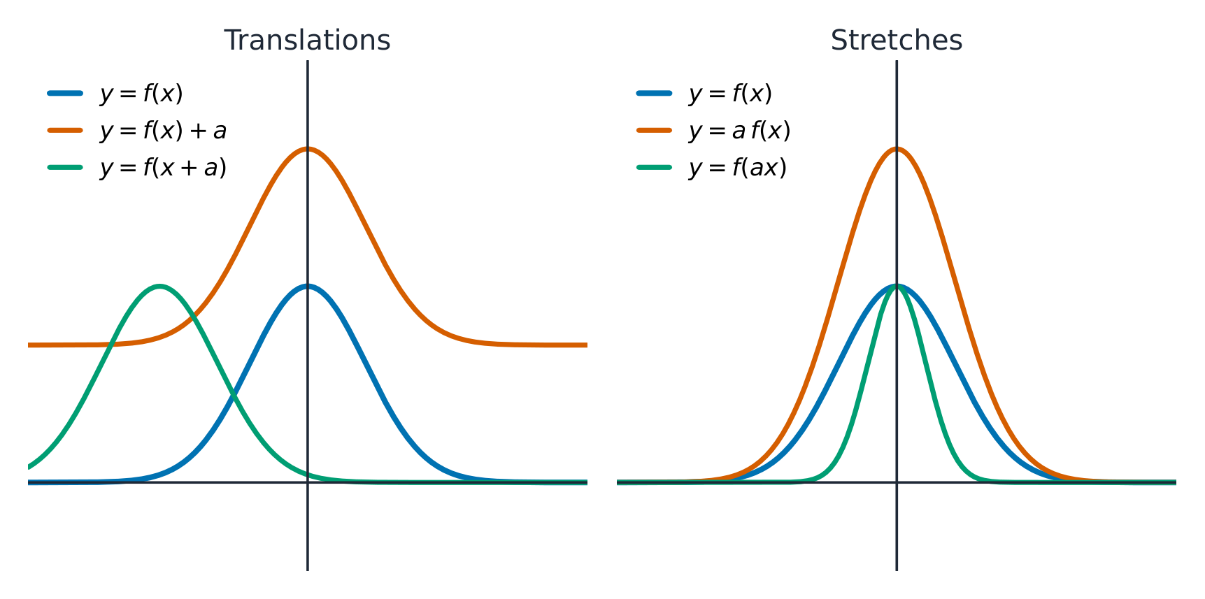
    Transformations of graphs

    A transformation 变换 builds a new function from an old one $f$:

    • Translations 平移 (shifts): $f(x)+k$ moves up/down; $f(x-h)$ moves right/left.
    • Dilations 伸缩 (stretches): $a\,f(x)$ stretches vertically; $f(bx)$ stretches horizontally.
    • Reflections 反射: $-f(x)$ flips over the $x$-axis; $f(-x)$ flips over the $y$-axis.

    Combine additive shifts and multiplicative stretches to model shifted, scaled versions of a known shape.

    ไทย
    การแปลงกราฟ

    การแปลง สร้างฟังก์ชันใหม่จากฟังก์ชันเก่า $f$:

    การบวกเข้าไปในเอาต์พุตหรืออินพุตทำให้กราฟเลื่อน; ตัวคูณทำให้กราฟยืด
    การบวกเข้าไปในเอาต์พุตหรืออินพุตทำให้กราฟเลื่อน; ตัวคูณทำให้กราฟยืด
    • การเลื่อน (shifts): $f(x)+k$ เลื่อนขึ้น/ลง; $f(x-h)$ เลื่อนขวา/ซ้าย.
    • การขยาย (stretches): $a\,f(x)$ ยืดในแนวตั้ง; $f(bx)$ ยืดในแนวนอน.
    • การสะท้อน: $-f(x)$ สะท้อนผ่านแกน $x$; $f(-x)$ สะท้อนผ่านแกน $y$.

    รวมการเลื่อนแบบบวกและการยืดแบบคูณเพื่อสร้างโมเดลสำหรับรูปทรงที่ทราบแล้วที่ถูกเลื่อนและปรับขนาด

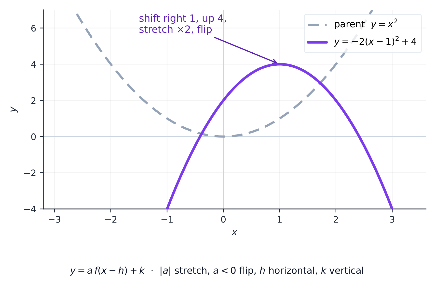
    การแปลงพาราโบลาต้นแบบ: เลื่อน, ยืด, และสะท้อน
    การแปลงพาราโบลาต้นแบบ: เลื่อน, ยืด, และสะท้อน
    Explore · ⁨สำรวจ⁩

    Explore shifts, stretches, and flips · ⁨สำรวจการเลื่อน การขยาย และการพลิก⁩

    Choose translate, reflect, rotate, or enlarge and change the amount. Watch which features stay the same — a transformation 变换 moves the whole graph without changing its underlying rule. · ⁨เลือก เลื่อน, สะท้อน, หมุน, หรือ ขยาย และปรับปริมาณ ดูว่าคุณลักษณะใดคงอยู่ — การแปลง 变换 ย้ายกราฟทั้งหมดโดยไม่เปลี่ยนกฎพื้นฐาน⁩

    Vocabulary · ⁨คำศัพท์⁩ Train · ⁨ฝึกฝน⁩
    English ไทย
    transformation/trænsfɔːˈmeɪʃn/ การแปรสภาพ
    Translations/trænˈsleɪʃnz/ การเลื่อน
    Dilations/daɪˈleɪʃnz/ การขยาย
    Reflections/rɪˈflekʃnz/ การสะท้อน
    model/ˈmɒdl/ แบบจำลอง
    assumptions/əˈsʌmpʃnz/ สมมติฐาน
    piecewise-defined function/ˈpiːswaɪz dɪˈfaɪnd ˈfʌŋkʃn/ ฟังก์ชันกำหนดทีละส่วน
    1.13

    Function Model Selection and Assumption Articulation · ⁨การเลือกโมเดลฟังก์ชันและการระบุสมมติฐาน⁩

    Syllabus · ⁨หลักสูตร⁩
    English

    Learning Objective 1.13.A: Identify an appropriate function type to construct a function model for a given scenario.

    • 1.13.A.1 Linear functions model data sets or aspects of contextual scenarios that demonstrate roughly constant rates of change.
    • 1.13.A.2 Quadratic functions model data sets or aspects of contextual scenarios that demonstrate roughly linear rates of change, or data sets that are roughly symmetric with a unique maximum or minimum value.
    • 1.13.A.3 Geometric contexts involving area or two dimensions can often be modeled by quadratic functions. Geometric contexts involving volume or three dimensions can often be modeled by cubic functions.
    • 1.13.A.4 Polynomial functions model data sets or contextual scenarios with multiple real zeros or multiple maxima or minima.
    • 1.13.A.5 A polynomial function of degree $n$ models data sets or contextual scenarios that demonstrate roughly constant nonzero $n$th differences.
    • 1.13.A.6 A polynomial function of degree $n$ or less can be used to model a graph of $n + 1$ points with distinct input values.
    • 1.13.A.7 A piecewise-defined function consists of a set of functions defined over nonoverlapping domain intervals and is useful for modeling a data set or contextual scenario that demonstrates different characteristics over different intervals.

    Learning Objective 1.13.B: Describe assumptions and restrictions related to building a function model.

    • 1.13.B.1 A model may have underlying assumptions about what is consistent in the model.
    • 1.13.B.2 A model may have underlying assumptions about how quantities change together.
    • 1.13.B.3 A model may require domain restrictions based on mathematical clues, contextual clues, or extreme values in the data set.
    • 1.13.B.4 A model may require range restrictions, such as rounding values, based on mathematical clues, contextual clues, or extreme values in the data set.
    ไทย

    วัตถุประสงค์การเรียนรู้ 1.13.A: ระบุประเภทของฟังก์ชันที่เหมาะสมเพื่อสร้างโมเดลฟังก์ชันสำหรับสถานการณ์ที่กำหนด

    • 1.13.A.1 ฟังก์ชันเชิงเส้นใช้จำลองชุดข้อมูลหรือองค์ประกอบของสถานการณ์ที่มีบริบทซึ่งแสดงอัตราการเปลี่ยนแปลงที่คงที่โดยประมาณ
    • 1.13.A.2 ฟังก์ชันกำลังสองใช้จำลองชุดข้อมูลหรือองค์ประกอบของสถานการณ์ที่มีบริบทซึ่งแสดงอัตราการเปลี่ยนแปลงที่เกือบเป็นเชิงเส้น หรือชุดข้อมูลที่มีความสมมาตรโดยประมาณและมีค่าสูงสุดหรือค่าต่ำสุดเพียงค่าเดียว
    • 1.13.A.3 สถานการณ์ทางเรขาคณิตที่เกี่ยวข้องกับพื้นที่หรือสองมิติ มักจะถูกจำลองด้วยฟังก์ชันกำลังสอง สถานการณ์ทางเรขาคณิตที่เกี่ยวข้องกับปริมาตรหรือสามมิติ มักจะถูกจำลองด้วยฟังก์ชันกำลังสาม
    • 1.13.A.4 ฟังก์ชันพหุนามจำลองชุดข้อมูลหรือสถานการณ์ในบริบทที่มีจุดศูนย์จริงหลายจุด หรือมีค่าสูงสุดหรือต่ำสุดหลายจุด
    • 1.13.A.5 ฟังก์ชันพหุนามของดีกรี $n$ จำลองชุดข้อมูลหรือสถานการณ์ในบริบทที่แสดงผลต่างระดับ $n$ ที่คงที่ประมาณการและไม่เป็นศูนย์
    • 1.13.A.6 ฟังก์ชันพหุนามที่มีดีกรี $n$ หรือน้อยกว่า สามารถใช้จำลองกราฟของ $n + 1$ จุดที่มีค่าอินพุตที่แตกต่างกัน
    • 1.13.A.7 ฟังก์ชันที่กำหนดแบบแบ่งช่วง (piecewise-defined function) ประกอบด้วยเซตของฟังก์ชันที่ถูกกำหนดบนช่วงโดเมนที่ไม่ทับซ้อนกัน และมีประโยชน์ในการจำลองชุดข้อมูลหรือสถานการณ์ในบริบทที่แสดงลักษณะที่แตกต่างกันในแต่ละช่วง
    วัตถุประสงค์การเรียนรู้ 1.13.B: อธิบายสมมติฐานและข้อจำกัดที่เกี่ยวข้องกับการสร้างโมเดลฟังก์ชัน

    • 1.13.B.1 โมเดลอาจมีสมมติฐานพื้นฐานเกี่ยวกับสิ่งที่คงที่ภายในโมเดล
    • 1.13.B.2 โมเดลอาจมีสมมติฐานพื้นฐานเกี่ยวกับวิธีการที่ปริมาณต่างๆ เปลี่ยนแปลงร่วมกัน
    • 1.13.B.3 โมเดลอาจต้องการข้อจำกัดของโดเมนโดยอ้างอิงจาก clues ทางคณิตศาสตร์, clues ในบริบท, หรือค่า extrems ในชุดข้อมูล
    • 1.13.B.4 โมเดลอาจต้องการข้อจำกัดของเรนจ์ เช่น การปัดเศษค่า โดยอ้างอิงจาก clues ทางคณิตศาสตร์, clues ในบริบท, หรือค่า extrems ในชุดข้อมูล

    Source: College Board AP Course and Exam Description · ⁨แหล่งที่มา: คำอธิบายหลักสูตรและข้อสอบ College Board AP⁩

    English

    Choosing a model 模型 means matching a function type to how a quantity changes. A linear model fits a constant rate of change; a quadratic fits a constant second difference; a polynomial fits data with several turns. In geometric situations the number of dimensions is a strong hint: quantities about area (two dimensions) are typically quadratic, and quantities about volume (three dimensions) are typically cubic – for example a box's volume as a function of a cut length. State the assumptions 假设 your model relies on (for example, that the pattern continues), because a model is only valid where those assumptions hold.

    ไทย

    การเลือก โมเดล หมายถึงการจับคู่ประเภทฟังก์ชันกับการเปลี่ยนแปลงของปริมาณ โมเดลเชิงเส้นเหมาะสำหรับการเปลี่ยนแปลงด้วยอัตราคงที่; โมเดลกำลังสองเหมาะสำหรับการต่างอันดับสองคงที่; พหุนามเหมาะกับข้อมูลที่มีหลายจุดเปลี่ยน ในสถานการณ์ทางเรขาคณิต จำนวนมิติเป็นข้อบ่งชี้ที่สำคัญ: ปริมาณเกี่ยวกับ พื้นที่ (สองมิติ) มักจะเป็น กำลังสอง, และปริมาณเกี่ยวกับ ปริมาตร (สามมิติ) มักจะเป็น กำลังสาม – ตัวอย่างเช่น ปริมาตรของกล่องในฐานะฟังก์ชันของความยาวตัด บอก สมมติฐาน ที่โมเดลของคุณพึ่งพา (เช่น, ว่ารูปแบบนี้ดำเนินต่อไป), เพราะโมเดลจะมีประโยชน์เฉพาะในพื้นที่ที่สมมติฐานเหล่านั้นเป็นจริง

    1.14

    Function Model Construction and Application · ⁨การสร้างและประยุกต์ใช้โมเดลฟังก์ชัน⁩

    Syllabus · ⁨หลักสูตร⁩
    English

    Learning Objective 1.14.A: Construct a linear, quadratic, cubic, quartic, polynomial of degree $n$, or related piecewise-defined function model.

    • 1.14.A.1 A model can be constructed based on restrictions identified in a mathematical or contextual scenario.
    • 1.14.A.2 A model of a data set or a contextual scenario can be constructed using transformations of the parent function.
    • 1.14.A.3 A model of a data set can be constructed using technology and regressions, including linear, quadratic, cubic, and quartic regressions.
    • 1.14.A.4 A piecewise-defined function model can be constructed through a combination of modeling techniques.

    Learning Objective 1.14.B: Construct a rational function model based on a context.

    • 1.14.B.1 Data sets and aspects of contextual scenarios involving quantities that are inversely proportional can often be modeled by rational functions. For example, the magnitudes of both gravitational force and electromagnetic force between objects are inversely proportional to the objects' squared distance.

    Learning Objective 1.14.C: Apply a function model to answer questions about a data set or contextual scenario.

    • 1.14.C.1 A model can be used to draw conclusions about the modeled data set or contextual scenario, including answering key questions and predicting values, rates of change, average rates of change, and changing rates of change. Appropriate units of measure should be extracted or inferred from the given context.
    ไทย

    วัตถุประสงค์การเรียนรู้ 1.14.A: สร้างโมเดลฟังก์ชันเชิงเส้น, ฟังก์ชันกำลังสอง, ฟังก์ชันกำลังสาม, ฟังก์ชันกำลังสี่, ฟังก์ชันพหุนามดีกรี $n$, หรือฟังก์ชันที่กำหนดแบบแบ่งช่วงที่เกี่ยวข้อง

    • 1.14.A.1 โมเดลสามารถสร้างได้โดยอ้างอิงจากข้อจำกัดที่ระบุได้ในสถานการณ์ทางคณิตศาสตร์หรือในบริบท
    • 1.14.A.2 โมเดลของชุดข้อมูลหรือสถานการณ์ในบริบทสามารถสร้างได้โดยใช้การแปลงของฟังก์ชันต้นแบบ (parent function)
    • 1.14.A.3 โมเดลของชุดข้อมูลสามารถสร้างได้ด้วยเทคโนโลยีและการถดถอย (regressions) รวมถึงการถดถอยเชิงเส้น, ฟังก์ชันกำลังสอง, ฟังก์ชันกำลังสาม, และการถดถอยกำลังสี่
    • 1.14.A.4 โมเดลฟังก์ชันที่กำหนดแบบแบ่งช่วงสามารถสร้างได้จากการผสมผสานเทคนิคการสร้างโมเดลต่างๆ

    วัตถุประสงค์การเรียนรู้ 1.14.B: สร้างโมเดลฟังก์ชันอัตราส่วนโดยอ้างอิงจากบริบท

    • 1.14.B.1 ชุดข้อมูลและด้านต่างๆ ของสถานการณ์ในบริบทที่เกี่ยวข้องกับปริมาณที่แปรผกผัน มักจะถูกจำลองด้วยฟังก์ชันอัตราส่วน ตัวอย่างเช่น ขนาดของแรงโน้มถ่วงและแรงแม่เหล็กไฟฟ้าระหว่างวัตถุแปรผกผันกับกำลังสองของระยะห่างระหว่างวัตถุนั้น

    วัตถุประสงค์การเรียนรู้ 1.14.C: ใช้โมเดลฟังก์ชันเพื่อตอบคำถามเกี่ยวกับชุดข้อมูลหรือสถานการณ์ในบริบท

    • 1.14.C.1 โมเดลสามารถใช้สรุปเกี่ยวกับชุดข้อมูลที่จำลองหรือสถานการณ์ในบริบทได้ รวมถึงการตอบคำถามสำคัญและการคาดการณ์ค่า อัตราการเปลี่ยนแปลง, อัตราการเปลี่ยนแปลงเฉลี่ย, และอัตราการเปลี่ยนแปลงของอัตราการเปลี่ยนแปลง ควรดึงหรืออนุมานหน่วยวัดที่เหมาะสมจากบริบทที่กำหนดให้

    Source: College Board AP Course and Exam Description · ⁨แหล่งที่มา: คำอธิบายหลักสูตรและข้อสอบ College Board AP⁩

    English

    To construct a model, use given features – points, intercepts, zeros with multiplicities, end behavior – to write the function, then use it to answer questions in context. Always check the answer against the domain that makes sense for the situation, and interpret outputs with their real-world units.

    A piecewise-defined function 分段函数 uses different rules over non-overlapping intervals of the domain. To evaluate it, pick the branch whose interval contains the input. For example,

    $$f(x)=\begin{cases} x^2, & x<0\\ 2x, & x\ge 0\end{cases}$$
    gives $f(-3)=9$ from the first branch but $f(3)=6$ from the second – useful when behaviour changes at a threshold (a tiered price, a speed limit that changes).

    ไทย

    เพื่อ สร้าง โมเดล, ใช้คุณสมบัติที่กำหนด – จุด, intercepts, จุดศูนย์พร้อมความซ้ำซ้อน, การ behaving ที่ปลาย – เพื่อเขียนฟังก์ชัน, จากนั้น用它ตอบคำถามในบริบท ตรวจสอบคำตอบเสมอเทียบกับ โดเมน ที่เหมาะสมกับสถานการณ์, และตีความเอาต์พุตด้วยหน่วยในโลกจริง

    ฟังก์ชันที่กำหนดแบบแบ่งส่วน ใช้กฎที่ต่างกันในช่วงที่ไม่ทับซ้อนกันของโดเมน ในการคำนวณค่า, เลือกสาขาwhose interval包含 the input. ตัวอย่าง,

    $$f(x)=\begin{cases} x^2, & x<0\\ 2x, & x\ge 0\end{cases}$$
    ให้ $f(-3)=9$ จากสาขาแรกแต่ $f(3)=6$ จากสาขาที่สอง – มีประโยชน์เมื่อพฤติกรรมเปลี่ยนที่เกณฑ์ (ราคาแบบขั้นบันได, ข้อจำกัดความเร็วที่เปลี่ยน)

    1.14

    Exam tips · ⁨ข้อแนะนำสำหรับการสอบ⁩

    English
    • Read a function through its rate of change: average rate = secant slope; a constant rate means linear, a linear-changing rate means quadratic.
    • Factor a polynomial to find zeros (x-intercepts) and their multiplicity; even multiplicity touches, odd crosses the axis.
    • End behaviour is set by the leading term; a rational function's asymptotes come from the degrees of top and bottom.
    • Build models from key features (points, zeros, end behaviour) and state your assumptions.
    • Describe transformations precisely: shift $f(x-h)+k$, stretch $af(bx)$, reflect $-f(x)$ / $f(-x)$.
    ไทย
    • อ่านฟังก์ชันผ่าน อัตราการเปลี่ยนแปลง: อัตราเฉลี่ย = ความชันของเส้นตัด; อัตราที่คงที่หมายถึงเชิงเส้น, อัตราที่เปลี่ยนเป็นเชิงเส้นหมายถึงกำลังสอง
    • แยกตัวประกอบพหุนามเพื่อหา จุดศูนย์ (จุดตัดแกน x) และระดับความซ้ำ; ระดับความซ้ำคู่สัมผัส, คี่ตัดผ่านแกน
    • พฤติกรรมปลายกำหนดโดย พจน์นำ; อสมการเชิงตรรกะมาจากดีกรีของตัวเศษและตัวส่วน
    • สร้างโมเดลจากคุณลักษณะสำคัญ (จุด, จุดศูนย์, พฤติกรรมปลาย) และระบุข้อสมมติฐานของคุณ
    • อธิบายการแปลงอย่างแม่นยำ: เลื่อน $f(x-h)+k$, ดึง $af(bx)$, สลับ $-f(x)$ / $f(-x)$.
  • 2

    Exponential and Logarithmic Functions · ⁨ฟังก์ชันเลขยกกำลังและลอการิทึม⁩

    Watch lesson · ⁨ดูบทเรียน⁩
    2.1

    Change in Arithmetic and Geometric Sequences · ⁨การเปลี่ยนแปลงในอนุกรมเลขคณิตและเรขาคณิต⁩

    Syllabus · ⁨หลักสูตร⁩
    English

    Learning Objective 2.1.A: Express arithmetic sequences found in mathematical and contextual scenarios as functions of the whole numbers.

    • 2.1.A.1 A sequence is a function from the whole numbers to the real numbers. Consequently, the graph of a sequence consists of discrete points instead of a curve.
    • 2.1.A.2 Successive terms in an arithmetic sequence have a common difference, or constant rate of change.
    • 2.1.A.3 The general term of an arithmetic sequence with a common difference $d$ is denoted by $a_n$ and is given by $a_n = a_0 + dn$, where $a_0$ is the initial value, or by $a_n = a_k + d(n - k)$, where $a_k$ is the $k$th term of the sequence.

    Learning Objective 2.1.B: Express geometric sequences found in mathematical and contextual scenarios as functions of the whole numbers.

    • 2.1.B.1 Successive terms in a geometric sequence have a common ratio, or constant proportional change.
    • 2.1.B.2 The general term of a geometric sequence with a common ratio $r$ is denoted by $g_n$ and is given by $g_n = g_0 r^n$, where $g_0$ is the initial value, or by $g_n = g_k r^{(n-k)}$, where $g_k$ is the $k$th term of the sequence.
    • 2.1.B.3 Increasing arithmetic sequences increase equally with each step, whereas increasing geometric sequences increase by a larger amount with each successive step.
    ไทย

    วัตถุประสงค์การเรียนรู้ 2.1.A: แสดงอนุกรมเลขคณิตที่พบในสถานการณ์ทางคณิตศาสตร์และบริบทต่างๆ ในรูปแบบฟังก์ชันของจำนวนเต็มบวก

    • 2.1.A.1 อนุกรม คือฟังก์ชันจากจำนวนเต็มบวกไปยังจำนวนจริง ดังนั้น กราฟของอนุกรมจึงประกอบด้วยจุดแยกต่างหากแทนที่จะเป็นเส้นโค้ง
    • 2.1.A.2 พจน์ติดกันในอนุกรมเลขคณิตมีผลต่างร่วม หรืออัตราการเปลี่ยนแปลงคงที่
    • 2.1.A.3 พจน์ทั่วไปของอนุกรมเลขคณิตที่มีผลต่าง $d$ แทนด้วย $a_n$ และกำหนดโดย $a_n = a_0 + dn$ โดยที่ $a_0$ เป็นค่าเริ่มต้น หรือโดย $a_n = a_k + d(n - k)$ โดยที่ $a_k$ เป็น $k$-พจน์ของอนุกรม

    วัตถุประสงค์การเรียนรู้ 2.1.B: แสดงอนุกรมเรขาคณิตที่พบในสถานการณ์ทางคณิตศาสตร์และบริบทต่างๆ ในรูปแบบฟังก์ชันของจำนวนเต็มบวก

    • 2.1.B.1 พจน์ติดกันในอนุกรมเรขาคณิตมีอัตราส่วนร่วม หรือการเปลี่ยนแปลงแบบสัดส่วนคงที่
    • 2.1.B.2 พจน์ทั่วไปของอนุกรมเรขาคณิตที่มีอัตราส่วน $r$ แทนด้วย $g_n$ และกำหนดโดย $g_n = g_0 r^n$ โดยที่ $g_0$ เป็นค่าเริ่มต้น หรือโดย $g_n = g_k r^{(n-k)}$ โดยที่ $g_k$ เป็น $k$-พจน์ของอนุกรม
    • 2.1.B.3 อนุกรมเลขคณิตที่เพิ่มขึ้นจะเพิ่มขึ้นเท่าๆ กันในแต่ละขั้นตอน ในขณะที่อนุกรมเรขาคณิตที่เพิ่มขึ้นจะเพิ่มขึ้นด้วยปริมาณที่มากขึ้นในแต่ละพจน์ถัดไป

    Source: College Board AP Course and Exam Description · ⁨แหล่งที่มา: คำอธิบายหลักสูตรและข้อสอบ College Board AP⁩

    English
    Geometric series & convergence

    A sequence 数列 is a function from the whole numbers to the real numbers, so its graph is discrete points, not a curve.

    • An arithmetic sequence 等差数列 has a common difference 公差 $d$ (a constant rate of change): $a_n = a_0 + dn$, or from a known term, $a_n = a_k + d(n-k)$.
    • A geometric sequence 等比数列 has a common ratio 公比 $r$ (a constant proportional change): $g_n = g_0\,r^{\,n}$, or $g_n = g_k\,r^{\,(n-k)}$.

    An increasing arithmetic sequence grows by the same amount each step; an increasing geometric sequence grows by a larger amount each step.

    Worked example. An arithmetic sequence with $a_0=3$ and $d=5$ has $a_4=3+5(4)=23$. A geometric sequence with $g_0=2$ and $r=3$ has $g_4=2\cdot3^4=162$ – addition versus multiplication makes the geometric one pull far ahead.

    ไทย
    อนุกรมเรขาคณิต & การลู่เข้า

    อนุกรมคือฟังก์ชันจากจำนวนเต็มบวกไปยังจำนวนจริง ดังนั้นกราฟของมันจึงเป็น จุดแยก ไม่ใช่เส้นโค้ง

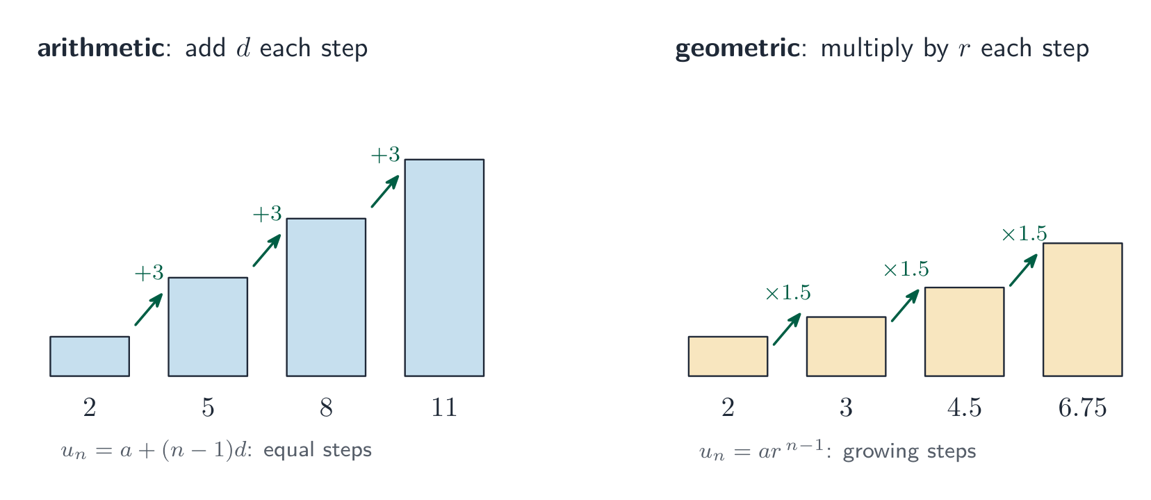
    อนุกรมเลขคณิตเพิ่มขึ้นทีละเท่ากัน; อนุกรมเรขาคณิตคูณด้วยอัตรา
    อนุกรมเลขคณิตเพิ่มขึ้นทีละเท่ากัน; อนุกรมเรขาคณิตคูณด้วยอัตรา
    • อนุกรมเลขคณิตมี ผลต่างร่วม $d$ (อัตราการเปลี่ยนแปลงคงที่): $a_n = a_0 + dn$, หรือจากพจน์ที่ทราบมา, $a_n = a_k + d(n-k)$.
    • อนุกรมเรขาคณิตมี อัตราส่วนร่วม $r$ (การเปลี่ยนแปลงตามสัดส่วนคงที่): $g_n = g_0\,r^{\,n}$, หรือ $g_n = g_k\,r^{\,(n-k)}$.

    อนุกรมเลขคณิตที่เพิ่มขึ้นเพิ่มใน ปริมาณเท่าเดิมทุกขั้นตอน; อนุกรมเรขาคณิตที่เพิ่มขึ้นเพิ่มใน ปริมาณมากขึ้นทุกขั้นตอน

    ตัวอย่างวิธีทำ. อนุกรมเลขคณิตที่มี $a_0=3$ และ $d=5$ มี $a_4=3+5(4)=23$. อนุกรมเรขาคณิตที่มี $g_0=2$ และ $r=3$ มี $g_4=2\cdot3^4=162$ – การบวกและการคูณทำให้แบบเรขาคณิตพุ่งไปข้างหน้าไกลกว่ามาก

    Explore · ⁨สำรวจ⁩

    Compare arithmetic and geometric growth · ⁨เปรียบเทียบการเติบโตแบบเลขคณิตและเรขาคณิต⁩

    An arithmetic sequence adds a fixed step each term (linear); a geometric sequence multiplies by a fixed ratio (exponential). Change the ratio and watch the terms explode or decay. · ⁨ลำดับเลขคณิต เพิ่มขั้นคงที่ในแต่ละพจน์ (เชิงเส้น); ลำดับเรขาคณิต คูณด้วยอัตราส่วนคงที่ (เอกซ์โพเนนเชียล) เปลี่ยนอัตราส่วนและดูพจน์ระเบิดหรือสลายตัว⁩

    2.2

    Change in Linear and Exponential Functions · ⁨การเปลี่ยนแปลงในฟังก์ชันเชิงเส้นและเอ็กซ์โพเนนเชียล⁩

    Syllabus · ⁨หลักสูตร⁩
    English

    Learning Objective 2.2.A: Construct functions of the real numbers that are comparable to arithmetic and geometric sequences.

    • 2.2.A.1 Linear functions of the form $f(x) = b + mx$ are similar to arithmetic sequences of the form $a_n = a_0 + dn$, as both can be expressed as an initial value ($b$ or $a_0$) plus repeated addition of a constant rate of change, the slope ($m$ or $d$).
    • 2.2.A.2 Similar to arithmetic sequences of the form $a_n = a_k + d(n - k)$, which are based on a known difference, $d$, and a $k$th term, linear functions can be expressed in the form $f(x) = y_i + m(x - x_i)$ based on a known slope, $m$, and a point, $(x_i, y_i)$.
    • 2.2.A.3 Exponential functions of the form $f(x) = ab^x$ are similar to geometric sequences of the form $g_n = g_0 r^n$, as both can be expressed as an initial value ($a$ or $g_0$) times repeated multiplication by a constant proportion ($b$ or $r$).
    • 2.2.A.4 Similar to geometric sequences of the form $g_n = g_k r^{(n-k)}$, which are based on a known ratio, $r$, and a $k$th term, exponential functions can be expressed in the form $f(x) = y_i r^{(x - x_i)}$ based on a known ratio, $r$, and a point, $(x_i, y_i)$.
    • 2.2.A.5 Sequences and their corresponding functions may have different domains.
    ไทย

    จุดประสงค์การเรียนรู้ 2.2.A: สร้างฟังก์ชันของจำนวนจริงที่เทียบเคียงได้กับอนุกรมเลขคณิตและอนุกรมเรขาคณิต

    • 2.2.A.1 ฟังก์ชันเชิงเส้นในรูป $f(x) = b + mx$ มีลักษณะคล้ายกับอนุกรมเลขคณิตในรูป $a_n = a_0 + dn$ เนื่องจากทั้งสองสามารถเขียนแทนค่าเป็นค่าเริ่มต้น ($b$ หรือ $a_0$) บวกด้วยการเพิ่มค่าคงที่ซ้ำๆ ซึ่งคืออัตราการเปลี่ยนแปลง, ความชัน ($m$ หรือ $d$)
    • 2.2.A.2 คล้ายกับอนุกรมเลขคณิตในรูป $a_n = a_k + d(n - k)$ ที่ตั้งอยู่บนผลต่าง Known, $d$, และ $k$ พจน์, ฟังก์ชันเชิงเส้นสามารถเขียนในรูป $f(x) = y_i + m(x - x_i)$ โดยอ้างอิงจากความชัน Known, $m$, และจุดหนึ่ง, $(x_i, y_i)$
    • 2.2.A.3 ฟังก์ชันเอกซ์โพเนนเชียลในรูป $f(x) = ab^x$ มีลักษณะคล้ายกับอนุกรมเรขาคณิตในรูป $g_n = g_0 r^n$ เนื่องจากทั้งสองสามารถเขียนแทนค่าเป็นค่าเริ่มต้น ($a$ หรือ $g_0$) คูณด้วยการคูณด้วยอัตราส่วนคงที่ซ้ำๆ ($b$ หรือ $r$)
    • 2.2.A.4 คล้ายกับอนุกรมเรขาคณิตในรูป $g_n = g_k r^{(n-k)}$ ที่ตั้งอยู่บนอัตราส่วน Known, $r$, และ $k$ พจน์, ฟังก์ชันเอกซ์โพเนนเชียลสามารถเขียนในรูป $f(x) = y_i r^{(x - x_i)}$ โดยอ้างอิงจากอัตราKnown, $r$, และจุดหนึ่ง, $(x_i, y_i)$
    • 2.2.A.5 อนุกรมและฟังก์ชันที่เกี่ยวข้องอาจมีโดเมนที่แตกต่างกัน

    Source: College Board AP Course and Exam Description · ⁨แหล่งที่มา: คำอธิบายหลักสูตรและข้อสอบ College Board AP⁩

    English

    Sequences have continuous cousins:

    • Linear functions $f(x)=b+mx$ mirror arithmetic sequences – an initial value plus repeated addition of the slope $m$. Point form: $f(x)=y_i+m(x-x_i)$.
    • Exponential functions $f(x)=ab^x$ mirror geometric sequences – an initial value times repeated multiplication by the base $b$. Point form: $f(x)=y_i\,r^{\,(x-x_i)}$.

    The difference: linear = repeated addition, exponential = repeated multiplication. (A sequence and its function may have different domains.)

    ไทย
    นักวิ่ง sprinter: โมเดลเอ็กซ์โพเนนเชียลและลอการิทึมจับอัตราการเติบโตและการลดลงในบริบท
    นักวิ่ง sprinter: โมเดลเอ็กซ์โพเนนเชียลและลอการิทึมจับอัตราการเติบโตและการลดลงในบริบท

    อนุกรมมีคู่Continuous:

    • ฟังก์ชันเชิงเส้น $f(x)=b+mx$ คล้ายกับอนุกรมเลขคณิต – ค่าเริ่มต้นบวกกับการเพิ่มซ้ำของความชัน $m$. รูปแบบจุด: $f(x)=y_i+m(x-x_i)$.
    • ฟังก์ชันเอ็กซ์โพเนนเชียล $f(x)=ab^x$ คล้ายกับอนุกรมเรขาคณิต – ค่าเริ่มต้นคูณด้วยการคูณซ้ำด้วยฐาน $b$. รูปแบบจุด: $f(x)=y_i\,r^{\,(x-x_i)}$.

    ความแตกต่าง: เชิงเส้น = การบวกซ้ำ, เอ็กซ์โพเนนเชียล = การคูณซ้ำ. (อนุกรมและฟังก์ชันอาจมีโดเมนต่างกัน)

    2.3

    Exponential Functions · ⁨ฟังก์ชันเอ็กซ์โพเนนเชียล⁩

    Syllabus · ⁨หลักสูตร⁩
    English

    Learning Objective 2.3.A: Identify key characteristics of exponential functions.

    • 2.3.A.1 The general form of an exponential function is $f(x) = ab^x$, with the initial value $a$, where $a \neq 0$, and the base $b$, where $b > 0$, and $b \neq 1$. When $a > 0$ and $b > 1$, the exponential function is said to demonstrate exponential growth. When $a > 0$ and $0 < b < 1$, the exponential function is said to demonstrate exponential decay.
    • 2.3.A.2 When the natural numbers are input values in an exponential function, the input value specifies the number of factors of the base to be applied to the function's initial value. The domain of an exponential function is all real numbers.
    • 2.3.A.3 Because the output values of exponential functions in general form are proportional over equal-length input-value intervals, exponential functions are always increasing or always decreasing, and their graphs are always concave up or always concave down. Consequently, exponential functions do not have extrema except on a closed interval, and their graphs do not have points of inflection.
    • 2.3.A.4 If the values of the additive transformation function $g(x) = f(x) + k$ of any function $f$ are proportional over equal-length input-value intervals, then $f$ is exponential.
    ไทย

    จุดประสงค์การเรียนรู้ 2.3.A: ระบุลักษณะสำคัญของฟังก์ชันเอกซ์โพเนนเชียล

    • 2.3.A.1 รูปแบบทั่วไปของฟังก์ชันเอกซ์โพเนนเชียลคือ $f(x) = ab^x$, โดยมี ค่าเริ่มต้น $a$, โดยที่ $a \neq 0$, และ ฐาน $b$, โดยที่ $b > 0$, และ $b \neq 1$ เมื่อ $a > 0$ และ $b > 1$, ฟังก์ชันเอกซ์โพเนนเชียลจะแสดงถึง การเติบโตแบบเอกซ์โพเนนเชียล เมื่อ $a > 0$ และ $0 < b < 1$, ฟังก์ชันเอกซ์โพเนนเชียลจะแสดงถึง การลดลงแบบเอกซ์โพเนนเชียล
    • 2.3.A.2 เมื่อจำนวนเต็มบวกเป็นค่าอินพุตในฟังก์ชันเอกซ์โพเนนเชียล ค่าอินพุตจะบ่งบอกจำนวนครั้งของการนำฐานไปคูณกับค่าเริ่มต้นของฟังก์ชัน โดเมนของฟังก์ชันเอกซ์โพเนนเชียลคือจำนวนจริงทั้งหมด
    • 2.3.A.3 เนื่องจากค่าเอาต์พุตของฟังก์ชันเอกซ์โพเนนเชียลในรูปแบบทั่วไปมีความสัมพันธ์กันในช่วงค่าอินพุตที่มีความยาวเท่ากัน ฟังก์ชันเอกซ์โพเนนเชียลจึงเพิ่มขึ้นหรือลดลงอย่างสม่ำเสมอเสมอ, และกราฟของมันจะโค้งขึ้นหรือโค้งลงอย่างสม่ำเสมอเสมอ ดังนั้น ฟังก์ชันเอกซ์โพเนนเชียลจึงไม่มีจุดสูงสุดหรือต่ำสุดยกเว้นบนช่วงปิด, และกราฟของมันไม่มีจุดเปลี่ยนเว้า
    • 2.3.A.4 หากค่าของฟังก์ชันการแปลงแบบบวก $g(x) = f(x) + k$ ของฟังก์ชันใดๆ $f$ มีความสัมพันธ์กันในช่วงค่าอินพุตที่มีความยาวเท่ากัน, แล้ว $f$ เป็นฟังก์ชันเอกซ์โพเนนเชียล

    Source: College Board AP Course and Exam Description · ⁨แหล่งที่มา: คำอธิบายหลักสูตรและข้อสอบ College Board AP⁩

    English

    The general exponential function 指数函数 is $f(x)=ab^x$ with initial value 初始值 $a\neq 0$ and base 底数 $b>0,\ b\neq 1$. Domain: all real numbers.

    • $a>0,\ b>1$ gives exponential growth 指数增长; $a>0,\ 0 gives exponential decay 指数衰减.
    • Outputs are proportional over equal-length input intervals. So an exponential is always increasing or always decreasing, and always concave up or always concave down – it has no extrema (except on a closed interval) and no points of inflection.
    ไทย

    ฟังก์ชันเอ็กซ์โพเนนเชียลทั่วไปคือ $f(x)=ab^x$ ที่มี ค่าเริ่มต้น $a\neq 0$ และ ฐาน $b>0,\ b\neq 1$. โดเมน: จำนวนจริงทั้งหมด

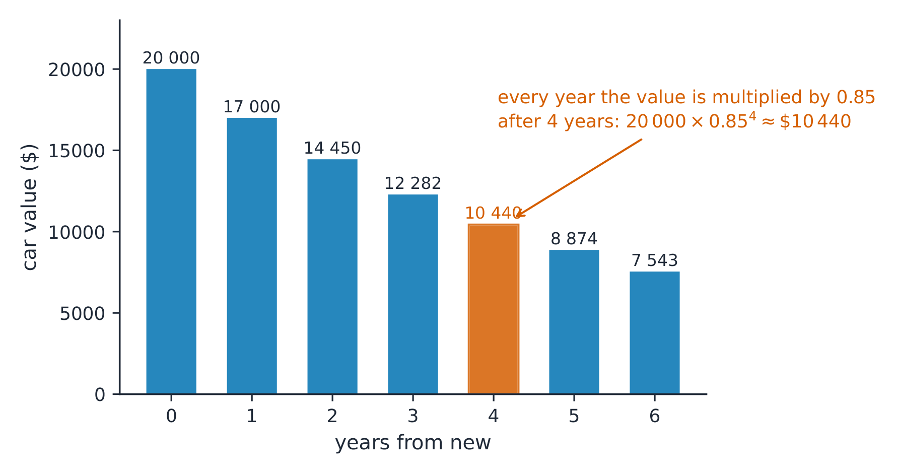
    การสลายตัวของเอ็กซ์โพเนนเชียล: เสียเปอร์เซ็นต์คงที่แต่ละรอบ
    การสลายตัวของเอ็กซ์โพเนนเชียล: เสียเปอร์เซ็นต์คงที่แต่ละรอบ
    • $a>0,\ b>1$ ให้ การเติบโตแบบเอ็กซ์โพเนนเชียล; $a>0,\ 0 ให้ การสลายตัวแบบเอ็กซ์โพเนนเชียล
    • ผลลัพธ์เป็น สัดส่วนในช่วงอินพุตที่มีความยาวเท่ากัน ดังนั้นเอ็กซ์โพเนนเชียลจึงเพิ่มขึ้นหรือลดลงตลอด และเว้าขึ้นหรือเว้าลงตลอด – ไม่มี จุดสุดขั้ว (ยกเว้นบนช่วงปิด) และไม่มี จุดเปลี่ยนเว้า
    แบคทีเรียภายใต้กล้องจุลทรรศน์: โมเดลเอ็กซ์โพเนนเชียลอธิบายประชากรที่เพิ่มขึ้นด้วยปัจจัยคงที่แต่ละขั้นตอนเวลา
    แบคทีเรียภายใต้กล้องจุลทรรศน์: โมเดลเอ็กซ์โพเนนเชียลอธิบายประชากรที่เพิ่มขึ้นด้วยปัจจัยคงที่แต่ละขั้นตอนเวลา
    Explore · ⁨สำรวจ⁩

    Explore an exponential curve · ⁨สำรวจเส้นโค้งเอกซ์โพเนนเชียล⁩

    y = a·e^(bx) + c

    An exponential function changes by a constant factor over equal steps, so it rises (or decays) ever faster. The constant $c$ sets the horizontal asymptote it hugs. · ⁨ฟังก์ชันเอกซ์โพเนนเชียล เปลี่ยนแปลงด้วย ตัวคูณ คงที่ในช่วงเท่ากัน จึงเพิ่มขึ้น (หรือลดลง) เร็วขึ้นเรื่อยๆ ค่าคงที่ $c$ กำหนดเส้น asymptote แนวนอนที่มันโอบอ้อม⁩

    Vocabulary · ⁨คำศัพท์⁩ Train · ⁨ฝึกฝน⁩
    English ไทย
    sequence/ˈsiːkwəns/ ลำดับขั้นตอน (sequence)
    arithmetic sequence/əˈrɪθmətɪk ˈsiːkwəns/ ลำดับเลขคณิต
    common difference/ˈkɒmən ˈdɪfrəns/ ผลต่างร่วม
    geometric sequence/ˌdʒiːəʊˈmetrɪk ˈsiːkwəns/ ลำดับเรขาคณิต
    common ratio/ˈkɒmən ˈreɪʃɪəʊ/ อัตราส่วนร่วม
    exponential function/ˌekspəˈnenʃl ˈfʌŋkʃn/ ฟังก์ชันเอ็กซ์โพเนนเชียล
    initial value/ɪˈnɪʃl ˈvæljuː/ ค่าเริ่มต้น
    base/beɪs/ ฐาน
    exponential growth/ˌekspəˈnenʃl ɡrəʊθ/ การเติบโตแบบเอกซ์โพเนนเชียล
    exponential decay/ˌekspəˈnenʃl dɪˈkeɪ/ การลดลงแบบเอกซ์โพเนนเชียล
    root/ruːt/ ราก
    exponential regression/ˌekspəˈnenʃl rɪˈɡreʃn/ การถดถอยเอ็กซ์โพเนนเชียล
    natural base/ˈnætʃərəl beɪs/ ฐานธรรมชาติ natural base
    residual plot/rɪˈsɪdʒuːəl plɒt/ แผนภูมิเศษเหลือ (residual plot)
    residual/rɪˈsɪdʒuːəl/ ค่าคงเหลือ
    composite function/ˈkɒmpəzɪt ˈfʌŋkʃn/ ฟังก์ชันประกอบ
    identity function/aɪˈdentɪti ˈfʌŋkʃn/ ฟังก์ชันเอกลักษณ์ identity function
    2.4

    Exponential Function Manipulation · ⁨การจัดการฟังก์ชันเอ็กซ์โพเนนเชียล⁩

    Syllabus · ⁨หลักสูตร⁩
    English

    Learning Objective 2.4.A: Rewrite exponential expressions in equivalent forms.

    • 2.4.A.1 The product property for exponents states that $b^m b^n = b^{(m+n)}$. Graphically, this property implies that every horizontal translation of an exponential function, $f(x) = b^{(x+k)}$, is equivalent to a vertical dilation, $f(x) = b^{(x+k)} = b^x b^k = ab^x$, where $a = b^k$.
    • 2.4.A.2 The power property for exponents states that $\left(b^m\right)^n = b^{(mn)}$. Graphically, this property implies that every horizontal dilation of an exponential function, $f(x) = b^{(cx)}$, is equivalent to a change of the base of an exponential function, $f(x) = \left(b^c\right)^x$, where $b^c$ is a constant and $c \neq 0$.
    • 2.4.A.3 The negative exponent property states that $b^{-n} = \dfrac{1}{b^n}$.
    • 2.4.A.4 The value of an exponential expression involving an exponential unit fraction, such as $b^{(1/k)}$ where $k$ is a natural number, is the $k$th root of $b$, when it exists.
    ไทย

    จุดประสงค์การเรียนรู้ 2.4.A: เขียนนิพจน์เอกซ์โพเนนเชียลใหม่ให้อยู่ในรูปที่เทียบเท่ากัน

    • 2.4.A.1 คุณสมบัติการคูณของเลขชี้กำลังระบุว่า $b^m b^n = b^{(m+n)}$ ในทางกราฟ, คุณสมบัตินี้บ่งบอกว่าทุกการเลื่อนแนวนอนของฟังก์ชันเอกซ์โพเนนเชียล, $f(x) = b^{(x+k)}$, เทียบเท่ากับ การขยายแนวตั้ง, $f(x) = b^{(x+k)} = b^x b^k = ab^x$, โดยที่ $a = b^k$
    • 2.4.A.2 คุณสมบัติการยกกำลังของเลขชี้กำลังระบุว่า $\left(b^m\right)^n = b^{(mn)}$ ในทางกราฟ, คุณสมบัตินี้บ่งบอกว่าทุกการขยายแนวนอนของฟังก์ชันเอกซ์โพเนนเชียล, $f(x) = b^{(cx)}$, เทียบเท่ากับการเปลี่ยนฐานของฟังก์ชันเอกซ์โพเนนเชียล, $f(x) = \left(b^c\right)^x$, โดยที่ $b^c$ เป็นค่าคงที่ และ $c \neq 0$
    • 2.4.A.3 คุณสมบัติเลขชี้กำลังลบระบุว่า $b^{-n} = \dfrac{1}{b^n}$
    • 2.4.A.4 ค่าของนิพจน์เอกซ์โพเนนเชียลที่ประกอบด้วยเศษส่วนเอกซ์โพเนนเชียล, เช่น $b^{(1/k)}$ โดยที่ $k$ เป็นจำนวนเต็มบวก, คือ รากที่ $k$ ของ $b$, เมื่อมันมีอยู่จริง

    Source: College Board AP Course and Exam Description · ⁨แหล่งที่มา: คำอธิบายหลักสูตรและข้อสอบ College Board AP⁩

    English

    The exponent rules reshape exponential expressions and connect to graph transformations:

    • Product: $b^m b^n = b^{m+n}$. A horizontal shift $b^{x+k}$ equals a vertical stretch $ab^x$ with $a=b^k$.
    • Power: $(b^m)^n = b^{mn}$. A horizontal stretch $b^{cx}$ equals a base change $(b^c)^x$.
    • Negative exponent: $b^{-n}=\dfrac{1}{b^n}$.
    • Unit-fraction exponent: $b^{1/k}=\sqrt[k]{b}$ (the $k$th root 方根).
    ไทย

    กฎเลขชี้กำลังปรับรูปนิพจน์เอ็กซ์โพเนนเชียลและเชื่อมต่อกับการแปลงกราฟ:

    • ผลคูณ: $b^m b^n = b^{m+n}$. การเลื่อนแนวนอน $b^{x+k}$ เท่ากับการดึงแนวตั้ง $ab^x$ ด้วย $a=b^k$.
    • กำลัง: $(b^m)^n = b^{mn}$. การดึงแนวนอน $b^{cx}$ เท่ากับการเปลี่ยนฐาน $(b^c)^x$.
    • เลขชี้กำลังลบ: $b^{-n}=\dfrac{1}{b^n}$.
    • เลขชี้กำลังเศษหน่วย: $b^{1/k}=\sqrt[k]{b}$ (รากที่ $k$).
    2.5

    Exponential Function Context and Data Modeling · ⁨บริบทและการสร้างโมเดลข้อมูลของฟังก์ชันเอ็กซ์โพเนนเชียล⁩

    Syllabus · ⁨หลักสูตร⁩
    English

    Learning Objective 2.5.A: Construct a model for situations involving proportional output values over equal-length input-value intervals.

    • 2.5.A.1 Exponential functions model growth patterns where successive output values over equal-length input-value intervals are proportional. When the input values are whole numbers, exponential functions model situations of repeated multiplication of a constant to an initial value.
    • 2.5.A.2 A constant may need to be added to the dependent variable values of a data set to reveal a proportional growth pattern.
    • 2.5.A.3 An exponential function model can be constructed from an appropriate ratio and initial value or from two input-output pairs. The initial value and the base can be found by solving a system of equations resulting from the two input-output pairs.
    • 2.5.A.4 Exponential function models can be constructed by applying transformations to $f(x) = ab^x$ based on characteristics of a contextual scenario or data set.
    • 2.5.A.5 Exponential function models can be constructed for a data set with technology using exponential regressions.
    • 2.5.A.6 The natural base $e$, which is approximately $2.718$, is often used as the base in exponential functions that model contextual scenarios.
    ไทย

    จุดประสงค์การเรียนรู้ 2.5.A: สร้างแบบจำลองสำหรับสถานการณ์ที่มีค่าเอาต์พุตแปรผันตามในช่วงค่าอินพุตที่มีความยาวเท่ากัน

    • 2.5.A.1 ฟังก์ชันเอกซ์โพเนนเชียลใช้สร้างแบบจำลองรูปแบบการเติบโตซึ่งค่าเอาต์พุตที่ต่อเนื่องกันในช่วงค่าอินพุตที่มีความยาวเท่ากันมีความสัมพันธ์กัน เมื่อค่าอินพุตเป็นจำนวนเต็ม ฟังก์ชันเอกซ์โพเนนเชียลใช้สร้างแบบจำลองสถานการณ์ของการคูณซ้ำๆ ของค่าคงที่กับค่าเริ่มต้น
    • 2.5.A.2 อาจจำเป็นต้องเพิ่มค่าคงที่ลงในค่าตัวแปรตามของชุดข้อมูลเพื่อเผยให้เห็นรูปแบบการเติบโตแบบแปรผัน
    • 2.5.A.3 สามารถสร้างแบบจำลองฟังก์ชันเอกซ์โพเนนเชียลได้จากอัตราส่วนที่เหมาะสมและค่าเริ่มต้น หรือจากคู่ค่าอินพุต-เอาต์พุตสองคู่ ค่าเริ่มต้นและฐานสามารถหาได้โดยการแก้ระบบสมการที่เกิดจากคู่ค่าอินพุต-เอาต์พุตสองคู่นั้น
    • 2.5.A.4 สามารถสร้างแบบจำลองฟังก์ชันเอกซ์โพเนนเชียลได้โดยนำการแปลงไปใช้กับ $f(x) = ab^x$ โดยอ้างอิงจากลักษณะของบริบทหรือชุดข้อมูล
    • 2.5.A.5 สามารถสร้างแบบจำลองฟังก์ชันเอกซ์โพเนนเชียลสำหรับชุดข้อมูลโดยใช้เทคโนโลยีผ่านการทำ Regression แบบเอกซ์โพเนนเชียล
    • 2.5.A.6 ฐานธรรมชาติ $e$ ซึ่งมีค่าประมาณ $2.718$ มักถูกใช้เป็นฐานในฟังก์ชันเอกซ์โพเนนเชียลที่สร้างแบบจำลองสถานการณ์ในบริบทต่างๆ

    Source: College Board AP Course and Exam Description · ⁨แหล่งที่มา: คำอธิบายหลักสูตรและข้อสอบ College Board AP⁩

    English

    Exponentials model quantities that grow by a constant proportion over equal intervals (repeated multiplication).

    • Build a model from a ratio and an initial value, or from two points (solve the system for $a$ and $b$).
    • Sometimes a constant must be added to the data to reveal the proportional pattern.
    • Use exponential regression 指数回归 on technology to fit a data set.
    • The natural base 自然底数 $e\approx 2.718$ is the standard base for real-world models.
    ไทย

    เอ็กซ์โพเนนเชียลสร้างโมเดลสำหรับปริมาณที่เพิ่มขึ้นด้วย สัดส่วนคงที่ในช่วงเท่ากัน (การคูณซ้ำ)

    • สร้างโมเดลจากอัตราและค่าเริ่มต้น, หรือจาก สองจุด (แก้ระบบสมการสำหรับ $a$ และ $b$).
    • บางครั้งต้อง เพิ่มค่าคงที่เข้ากับข้อมูลเพื่อเผยให้เห็นรูปแบบสัดส่วน
    • ใช้ การถดถอยเอ็กซ์โพเนนเชียลบนเทคโนโลยีเพื่อจับชุดข้อมูล
    • ฐานธรรมชาติ $e\approx 2.718$ เป็นฐานมาตรฐานสำหรับโมเดลในโลกจริง
    2.6

    Competing Function Model Validation · ⁨การตรวจสอบโมเดลฟังก์ชันที่แข่งขันกัน⁩

    Syllabus · ⁨หลักสูตร⁩
    English

    Learning Objective 2.6.A: Construct linear, quadratic, and exponential models based on a data set.

    • 2.6.A.1 Two variables in a data set that demonstrate a slightly changing rate of change can be modeled by linear, quadratic, and exponential function models.
    • 2.6.A.2 Models can be compared based on contextual clues and applicability to determine which model is most appropriate.

    Learning Objective 2.6.B: Validate a model constructed from a data set.

    • 2.6.B.1 A model is justified as appropriate for a data set if the graph of the residuals of a regression, the residual plot, appear without pattern.
    • 2.6.B.2 The difference between the predicted and actual values is the error in the model. Depending on the data set and context, it may be more appropriate to have an underestimate or overestimate for any given interval.
    ไทย

    จุดประสงค์การเรียนรู้ 2.6.A: สร้างแบบจำลองเชิงเส้น, สี่เหลี่ยมจตุรัส, และเอกซ์โพเนนเชียลโดยอ้างอิงจากชุดข้อมูล

    • 2.6.A.1 ตัวแปรสองตัวในชุดข้อมูลที่แสดงอัตราการเปลี่ยนแปลงที่เปลี่ยนแปลงเล็กน้อยสามารถสร้างแบบจำลองได้ด้วยฟังก์ชันเชิงเส้น, สี่เหลี่ยมจตุรัส, และเอกซ์โพเนนเชียล
    • 2.6.A.2 สามารถเปรียบเทียบแบบจำลองได้โดยอ้างอิงจากข้อบ่งชี้ในบริบทและความเหมาะสมเพื่อกำหนดว่าแบบจำลองใดเหมาะสมที่สุด

    จุดประสงค์การเรียนรู้ 2.6.B: ตรวจสอบความถูกต้องของแบบจำลองที่สร้างขึ้นจากชุดข้อมูล

    • 2.6.B.1 โมเดลจะถือว่า เหมาะสม กับชุดข้อมูลหากกราฟของค่าคงเหลือจากการถดถอย (residual plot) ปรากฏโดยไม่มีการจัดเรียงรูปแบบ
    • 2.6.B.2 ความแตกต่างระหว่างค่าที่คาดหมายและค่าจริงคือ ความคลาดเคลื่อน ในโมเดล ขึ้นอยู่กับชุดข้อมูลและบริบท อาจเหมาะสมกว่าที่จะมีค่าประมาณต่ำกว่าหรือสูงกว่าสำหรับช่วงใดช่วงหนึ่ง

    Source: College Board AP Course and Exam Description · ⁨แหล่งที่มา: คำอธิบายหลักสูตรและข้อสอบ College Board AP⁩

    English

    When a rate of change shifts only slightly, linear, quadratic, and exponential models may all seem to fit. Choose using context and fit quality:

    • A model is appropriate if its residual plot 残差图 shows no pattern (a residual 残差 is actual minus predicted).
    • The error is the gap between predicted and actual; context decides whether an over- or under-estimate is safer.
    ไทย

    เมื่ออัตราการเปลี่ยนแปลงเปลี่ยนเพียงเล็กน้อย โมเดลเชิงเส้น กำลังสอง และเอ็กซ์โพเนนเชียลอาจดูว่าเข้ากันทั้งนั้น เลือกโดยใช้บริบทและคุณภาพของการเข้ากัน:

    • โมเดล เหมาะสมหาก แผนภาพค่าตกค้างแสดง ไม่มีรูปแบบ (ค่าตกค้างคือค่าจริงลบด้วยค่าคาดหมาย)
    • ความผิดพลาดคือช่องว่างระหว่างค่าคาดหมายกับค่าจริง; บริบทตัดสินใจว่าค่าประมาณเกินหรือต่ำกว่า哪个ปลอดภัยกว่า
    2.7

    Composition of Functions · ⁨การประกอบฟังก์ชัน⁩

    Syllabus · ⁨หลักสูตร⁩
    English

    Learning Objective 2.7.A: Evaluate the composition of two or more functions for given values.

    • 2.7.A.1 If $f$ and $g$ are functions, the composite function $f \circ g$ maps a set of input values to a set of output values such that the output values of $g$ are used as input values of $f$. For this reason, the domain of the composite function is restricted to those input values of $g$ for which the corresponding output value is in the domain of $f$. $(f \circ g)(x)$ can also be represented as $f(g(x))$.
    • 2.7.A.2 Values for the composite function $f \circ g$ can be calculated or estimated from the graphical, numerical, analytical, or verbal representations of $f$ and $g$ by using output values from $g$ as input values for $f$.
    • 2.7.A.3 The composition of functions is not commutative; that is, $f \circ g$ and $g \circ f$ are typically different functions; therefore, $f(g(x))$ and $g(f(x))$ are typically different values.
    • 2.7.A.4 If the function $f(x) = x$ is composed with any function $g$, the resulting composite function is the same as $g$; that is, $g(f(x)) = f(g(x)) = g(x)$. The function $f(x) = x$ is called the identity function. When composing two functions, the identify function acts in the same way as $0$, the additive identity, when adding two numbers and $1$, the multiplicative identity, when multiplying two numbers.

    Learning Objective 2.7.B: Construct a representation of the composition of two or more functions.

    • 2.7.B.1 Function composition is useful for relating two quantities that are not directly related by an existing formula.
    • 2.7.B.2 When analytic representations of the functions $f$ and $g$ are available, an analytic representation of $f(g(x))$ can be constructed by substituting $g(x)$ for every instance of $x$ in $f$.
    • 2.7.B.3 A numerical or graphical representation of $f \circ g$ can often be constructed by calculating or estimating values for $(x, f(g(x)))$.

    Learning Objective 2.7.C: Rewrite a given function as a composition of two or more functions.

    • 2.7.C.1 Functions given analytically can often be decomposed into less complicated functions. When properly decomposed, the variable in one function should replace each instance of the function with which it was composed.
    • 2.7.C.2 An additive transformation of a function, $f$, that results in vertical and horizontal translations can be understood as the composition of $g(x) = x + k$ with $f$.
    • 2.7.C.3 A multiplicative transformation of a function, $f$, that results in vertical and horizontal dilations can be understood as the composition of $g(x) = kx$ with $f$.
    ไทย

    จุดประสงค์การเรียนรู้ 2.7.A: ประเมินการประกอบของสองหรือมากกว่าฟังก์ชันสำหรับค่าที่กำหนดให้

    • 2.7.A.1 หาก $f$ และ $g$ เป็นฟังก์ชัน ฟังก์ชันประกอบ $f \circ g$ จะจับคู่เซตของค่าอินพุตเข้ากับเซตของค่าเอาต์พุต โดยที่ค่าเอาต์พุตของ $g$ จะถูกใช้เป็นค่าอินพุตของ $f$ ด้วยเหตุนี้โดเมนของฟังก์ชันประกอบจึงถูกจำกัดไว้เฉพาะค่าอินพุตของ $g$ ที่ค่าเอาต์พุตที่เกี่ยวข้องอยู่ในโดเมนของ $f$ $(f \circ g)(x)$ ยังสามารถแสดงในรูปแบบ $f(g(x))$ ได้
    • 2.7.A.2 ค่าของฟังก์ชันประกอบ $f \circ g$ สามารถคำนวณหรือประมาณได้จากการแทนค่ากราฟ ตัวเลข สมการ หรือคำอธิบายของ $f$ และ $g$ โดยใช้ค่าเอาต์พุตจาก $g$ เป็นค่าอินพุตสำหรับ $f$
    • 2.7.A.3 การประกอบฟังก์ชันไม่เป็นแบบสลับที่ได้ (non-commutative) นั่นคือ $f \circ g$ และ $g \circ f$ มักจะเป็นฟังก์ชันที่แตกต่างกัน ดังนั้น $f(g(x))$ และ $g(f(x))$ จึงมักเป็นค่าที่แตกต่างกัน
    • 2.7.A.4 หากฟังก์ชัน $f(x) = x$ ถูกประกอบกับฟังก์ชันใดๆ $g$ ฟังก์ชันประกอบที่เกิดขึ้นจะมีค่าเท่ากับ $g$ เสมอ นั่นคือ $g(f(x)) = f(g(x)) = g(x)$ ฟังก์ชัน $f(x) = x$ เรียกว่า ฟังก์ชันเอกลักษณ์ (identity function) เมื่อประกอบฟังก์ชันสองตัว ฟังก์ชันเอกลักษณ์จะทำหน้าที่เหมือน $0$ ซึ่งเป็นเอกลักษณ์ของการบวกเมื่อเพิ่มจำนวนสองจำนวน และ $1$ ซึ่งเป็นเอกลักษณ์ของการคูณเมื่อคูณจำนวนสองจำนวน

    จุดประสงค์การเรียนรู้ 2.7.B: สร้างการแสดงผลของการประกอบของสองหรือมากกว่าฟังก์ชัน

    • 2.7.B.1 การประกอบฟังก์ชันมีประโยชน์สำหรับการเชื่อมโยงปริมาณสองอย่างที่ไม่ได้สัมพันธ์กันโดยตรงผ่านสูตรที่มีอยู่เดิม
    • 2.7.B.2 เมื่อมีรูปแบบสมการของฟังก์ชัน $f$ และ $g$ อยู่แล้ว สามารถสร้างรูปแบบสมการของ $f(g(x))$ ได้โดยการแทนค่า $g(x)$ เข้าไปในทุกตำแหน่งของ $x$ ใน $f$
    • 2.7.B.3 การแสดงค่าตัวเลขหรือกราฟของ $f \circ g$ มักสามารถสร้างได้ด้วยการคำนวณหรือประมาณค่าของ $(x, f(g(x)))$

    จุดประสงค์การเรียนรู้ 2.7.C: เขียนฟังก์ชันที่กำหนดให้ใหม่ในรูปของการประกอบของสองหรือมากกว่าฟังก์ชัน

    • 2.7.C.1 ฟังก์ชันที่กำหนดด้วยสมการมักสามารถแยกองค์ประกอบออกเป็นฟังก์ชันที่ซับซ้อนน้อยลง เมื่อแยกองค์ประกอบได้อย่างถูกต้อง ตัวแปรในฟังก์ชันหนึ่งควรไปแทนที่ทุกตำแหน่งของฟังก์ชันที่ถูกประกอบเข้าด้วยกัน
    • 2.7.C.2 การแปลงเชิงบวกของฟังก์ชัน $f$ ซึ่งส่งผลให้เกิดการเลื่อนแนวตั้งและแนวนอน สามารถเข้าใจได้ว่าเป็นการประกอบของ $g(x) = x + k$ กับ $f$
    • 2.7.C.3 การแปลงคูณของฟังก์ชัน $f$ ที่ทำให้เกิดการขยายแนวตั้งและแนวนอน สามารถอธิบายได้ว่าเป็นการประกอบกันของ $g(x) = kx$ กับ $f$

    Source: College Board AP Course and Exam Description · ⁨แหล่งที่มา: คำอธิบายหลักสูตรและข้อสอบ College Board AP⁩

    English

    The composite function 复合函数 $(f\circ g)(x)=f(g(x))$ feeds $g$'s output into $f$. Its domain is the inputs of $g$ whose outputs lie in $f$'s domain.

    • Composition is not commutative: $f(g(x))$ and $g(f(x))$ usually differ.
    • To build $f(g(x))$ analytically, substitute $g(x)$ for every $x$ in $f$.
    • The identity function 恒等函数 $f(x)=x$ leaves any function unchanged under composition.
    • A function can also be decomposed into simpler pieces – useful for seeing an additive shift as composing with $x+k$, or a dilation as composing with $kx$.
    ไทย

    ฟังก์ชันประกอบ $(f\circ g)(x)=f(g(x))$ นำผลลัพธ์ของ $g$ ไปใส่ใน $f$. โดเมนของมันคืออินพุตของ $g$ ที่ผลลัพธ์อยู่ในโดเมนของ $f$

    ฟังก์ชันเป็นเครื่องจักร; ฟังก์ชันผกผัน运行的เครื่องกลับ backwards
    ฟังก์ชันเป็นเครื่องจักร; ฟังก์ชันผกผัน运行的เครื่อง backwards
    • การประกอบ ไม่มีการแลกเปลี่ยน: $f(g(x))$ และ $g(f(x))$ โดยทั่วไปจะต่างกัน
    • เพื่อสร้าง $f(g(x))$ แบบวิเคราะห์, แทนที่ $g(x)$ แทน $x$ ทุกตัวใน $f$
    • ฟังก์ชันเอกลักษณ์ $f(x)=x$ ทำให้ฟังก์ชันใดๆ ไม่เปลี่ยนภายใต้การประกอบ
    • ฟังก์ชันยังสามารถ แยกส่วนออกเป็นชิ้นส่วนที่ง่ายขึ้น – มีประโยชน์สำหรับการเห็นการเลื่อนเชิงบวกเป็นการประกอบกับ $x+k$, หรือการขยายเป็นการประกอบกับ $kx$
    ตุ๊กตา Matryoshka: การประกอบฟังก์ชันซ้อนชั้น – คำนวณด้านในก่อน
    ตุ๊กตา Matryoshka: การประกอบฟังก์ชันซ้อนชั้น – คำนวณด้านในก่อน
    2.8

    Inverse Functions · ⁨ฟังก์ชันผกผัน⁩

    Syllabus · ⁨หลักสูตร⁩
    Learning ObjectiveEssential Knowledge

    2.8.A
    Determine the input-output pairs of the inverse of a function.

    • 2.8.A.1 On a specified domain, a function, $f$, has an inverse function, or is invertible, if each output value of $f$ is mapped from a unique input value. The domain of a function may be restricted in many ways to make the function invertible.
    • 2.8.A.2 An inverse function can be thought of as a reverse mapping of the function. An inverse function, $f^{-1}$, maps the output values of a function, $f$, on its invertible domain to their corresponding input values; that is, if $f(a) = b$, then $f^{-1}(b) = a$. Alternately, on its invertible domain, if a function consists of input-output pairs $(a, b)$, then the inverse function consists of input-output pairs $(b, a)$.

    2.8.B
    Determine the inverse of a function on an invertible domain.

    • 2.8.B.1 The composition of a function, $f$, and its inverse function, $f^{-1}$, is the identity function; that is, $f\left(f^{-1}(x)\right) = f^{-1}(f(x)) = x$.
    • 2.8.B.2 On a function's invertible domain, the function's range and domain are the inverse function's domain and range, respectively. The inverse of the table of values of $y = f(x)$ can be found by reversing the input-output pairs; that is, $(a, b)$ corresponds to $(b, a)$.
    • 2.8.B.3 The inverse of the graph of the function $y = f(x)$ can be found by reversing the roles of the $x$- and $y$-axes; that is, by reflecting the graph of the function over the graph of the identity function $h(x) = x$.
    • 2.8.B.4 The inverse of the function can be found by determining the inverse operations to reverse the mapping. One method for finding the inverse of the function $f$ is reversing the roles of $x$ and $y$ in the equation $y = f(x)$, then solving for $y = f^{-1}(x)$.
    • 2.8.B.5 In addition to limiting the domain of a function to obtain an inverse function, contextual restrictions may also limit the applicability of an inverse function.

    Source: College Board AP Course and Exam Description · ⁨แหล่งที่มา: คำอธิบายหลักสูตรและข้อสอบ College Board AP⁩

    English
    Inverse functions are a reflection
    Exponential & logarithm are inverses

    A function is invertible 可逆 on a domain where each output comes from a unique input (you may restrict the domain to force this). The inverse function 反函数 $f^{-1}$ reverses the mapping: if $f(a)=b$ then $f^{-1}(b)=a$.

    • $f\big(f^{-1}(x)\big)=f^{-1}\big(f(x)\big)=x$ (composition gives the identity).
    • Domain and range swap: reverse each $(a,b)$ to $(b,a)$ in a table; reflect the graph over the line $y=x$.
    • To find a formula: swap $x$ and $y$ in $y=f(x)$, then solve for $y$. Context may further limit where the inverse applies.
    ไทย
    ฟังก์ชันผกผันเป็นการสะท้อน
    Exponential & logarithm are inverses

    ฟังก์ชันหนึ่งๆ จะ ผกผันได้ (invertible) ในโดเมนที่แต่ละค่าผลลัพธ์มาจาก ตัวแปรเข้าที่เฉพาะเจาะจง (คุณสามารถจำกัดโดเมนเพื่อบังคับให้เป็นเช่นนั้น) ฟังก์ชันผกผัน $f^{-1}$ ทำการย้อนกลับการจับคู่: หาก $f(a)=b$ แล้ว $f^{-1}(b)=a$

    • $f\big(f^{-1}(x)\big)=f^{-1}\big(f(x)\big)=x$ (การประกอบให้ผลลัพธ์เป็นเอกลักษณ์)
    • โดเมนและเรนจ์ สลับกัน: ย้อนกลับ $(a,b)$ เป็น $(b,a)$ ในตาราง; สะท้อนกราฟผ่านเส้นตรง $y=x$
    • การหาคำอธิบายทางคณิตศาสตร์: สลับ $x$ และ $y$ ใน $y=f(x)$ จากนั้นแก้สมการหา $y$. บริบทอาจจำกัดเพิ่มเติมว่าฟังก์ชันผกผันใช้ได้ในช่วงใดบ้าง
    Vocabulary · ⁨คำศัพท์⁩ Train · ⁨ฝึกฝน⁩
    English ไทย
    invertible/ɪnˈvɜːtɪbl/ สามารถกลับด้านได้ invertible
    inverse function/ɪnˈvɜːs ˈfʌŋkʃn/ ฟังก์ชันผกผัน
    logarithm/ˈlɒɡərɪθəm/ ลอการิทึม
    common logarithm/ˈkɒmən ˈlɒɡərɪθəm/ ลอการิทึมฐานสิบ common logarithm
    natural logarithm/ˈnætʃərəl ˈlɒɡərɪθəm/ ลอการิทึมธรรมชาติ
    logarithmic function/ˌlɒɡəˈrɪθmɪk ˈfʌŋkʃn/ ฟังก์ชันลอการิทึม
    change-of-base/tʃeɪndʒ ɒv beɪs/ change-of-base (换底公式)
    semi-log plot/ˈsemi lɒɡ plɒt/ กราฟ semi-log
    2.9

    Logarithmic Expressions · ⁨นิพจน์ลอการิทึม⁩

    Syllabus · ⁨หลักสูตร⁩
    English

    Learning Objective 2.9.A: Evaluate logarithmic expressions.

    • 2.9.A.1 The logarithmic expression $\log_b c$ is equal to, or represents, the value that the base $b$ must be exponentially raised to in order to obtain the value $c$. That is, $\log_b c = a$ if and only if $b^a = c$, where $a$ and $c$ are constants, $b > 0$, and $b \neq 1$. (when the base of a logarithmic expression is not specified, it is understood as the common logarithm with a base of $10$)
    • 2.9.A.2 The values of some logarithmic expressions are readily accessible through basic arithmetic while other values can be estimated through the use of technology.
    • 2.9.A.3 On a logarithmic scale, each unit represents a multiplicative change of the base of the logarithm. For example, on a standard scale, the units might be $0, \; 1, \; 2, \; \ldots$, while on a logarithmic scale, using logarithm base $10$, the units might be $10^0, \; 10^1, \; 10^2, \; \ldots$.
    ไทย

    จุดประสงค์การเรียนรู้ 2.9.A: ประเมินนิพจน์ลอการิทึม

    • 2.9.A.1 นิพจน์ลอการิทึม $\log_b c$ เท่ากับ หรือแทนค่าของเลขชี้กำลังที่ฐาน $b$ ต้องถูกยกกำลังเพื่อให้ได้ค่า $c$ นั่นคือ $\log_b c = a$ ก็ต่อเมื่อ $b^a = c$ โดยที่ $a$ และ $c$ เป็นค่าคงที่, $b > 0$, และ $b \neq 1$ (เมื่อไม่ระบุฐานของนิพจน์ลอการิทึม จะ理解为เป็นลอการิทึมทั่วไปที่มีฐาน $10$)
    • 2.9.A.2 ค่าของนิพจน์ลอการิทึมบางชนิดสามารถหาได้จาก arithmetic พื้นฐาน ในขณะที่ค่าอื่นๆ สามารถประมาณได้โดยใช้ technology
    • 2.9.A.3 บนสเกลลอการิทึม แต่ละหน่วยจะแสดงถึงการเปลี่ยนแปลงแบบคูณด้วยฐานของลอการิทึม เช่น บนสเกลมาตรฐาน หน่วยอาจเป็น $0, \; 1, \; 2, \; \ldots$ แต่บนสเกลลอการิทึม โดยใช้ฐานลอการิทึม $10$ หน่วยอาจเป็น $10^0, \; 10^1, \; 10^2, \; \ldots$

    Source: College Board AP Course and Exam Description · ⁨แหล่งที่มา: คำอธิบายหลักสูตรและข้อสอบ College Board AP⁩

    English

    The logarithm 对数 answers "what exponent?": $\log_b c = a$ means exactly $b^a = c$ (with $b>0,\ b\neq 1$). An unwritten base means the common logarithm 常用对数 (base $10$). On a logarithmic scale, each unit is a multiplicative step of the base (…, $10^0,10^1,10^2,$ …).

    ไทย

    ลอการิทึมตอบคำถาม "เลขชี้กำลังคืออะไร?": $\log_b c = a$ หมายความว่า $b^a = c$ พอดี (โดยมี $b>0,\ b\neq 1$). การไม่เขียนฐานไว้แสดงว่าเป็น ลอการิทึมทั่วไป (ฐาน $10$). บน สเกลลอการิทึม แต่ละหน่วยคือขั้นตอนการคูณด้วยฐาน (... $10^0,10^1,10^2,$ ...)

    2.10

    Inverses of Exponential Functions · ⁨ฟังก์ชันผกผันของฟังก์ชันเอ็กซ์โพเนนเชียล⁩

    Syllabus · ⁨หลักสูตร⁩
    English

    Learning Objective 2.10.A: Construct representations of the inverse of an exponential function with an initial value of 1.

    • 2.10.A.1 The general form of a logarithmic function is $f(x) = a\log_b x$, with base $b$, where $b > 0$, $b \neq 1$, and $a \neq 0$.
    • 2.10.A.2 The way in which input and output values vary together have an inverse relationship in exponential and logarithmic functions. Output values of general-form exponential functions change proportionately as input values increase in equal-length intervals. However, input values of general-form logarithmic functions change proportionately as output values increase in equal-length intervals. Alternately, exponential growth is characterized by output values changing multiplicatively as input values change additively, whereas logarithmic growth is characterized by output values changing additively as input values change multiplicatively.
    • 2.10.A.3 $f(x) = \log_b x$ and $g(x) = b^x$, where $b > 0$ and $b \neq 1$, are inverse functions. That is, $g(f(x)) = f(g(x)) = x$.
    • 2.10.A.4 The graph of the logarithmic function $f(x) = \log_b x$, where $b > 0$ and $b \neq 1$, is a reflection of the graph of the exponential function $g(x) = b^x$, where $b > 0$ and $b \neq 1$, over the graph of the identity function $h(x) = x$.
    • 2.10.A.5 If $(s, \; t)$ is an ordered pair of the exponential function $g(x) = b^x$, where $b > 0$ and $b \neq 1$, then $(t, \; s)$ is an ordered pair of the logarithmic function $f(x) = \log_b x$, where $b > 0$ and $b \neq 1$.
    ไทย

    วัตถุประสงค์การเรียนรู้ 2.10.A: สร้างการแสดงภาพของฟังก์ชันผกผันของฟังก์ชันเอ็กซ์โพเนนเชียลที่มีค่าเริ่มต้นเป็น 1

    • 2.10.A.1 รูปแบบทั่วไปของฟังก์ชันลอการิทึมคือ $f(x) = a\log_b x$ โดยมีฐาน $b$ โดยที่ $b > 0$, $b \neq 1$ และ $a \neq 0$
    • 2.10.A.2 วิธีการที่ค่าอินพุตและเอาต์พุตแปรผันร่วมกันมีความสัมพันธ์ผกผันในฟังก์ชันเอ็กซ์โพเนนเชียลและลอการิทึม ค่าเอาต์พุตของฟังก์ชันเอ็กซ์โพเนนเชียลรูปแบบทั่วไปเปลี่ยนแบบสัดส่วนเมื่อค่าอินพุตเพิ่มขึ้นในช่วงความยาวเท่ากัน อย่างไรก็ตาม ค่าอินพุตของฟังก์ชันลอการิทึมรูปแบบทั่วไปเปลี่ยนแบบสัดส่วนเมื่อค่าเอาต์พุตเพิ่มขึ้นในช่วงความยาวเท่ากัน ทางเลือกอื่น การเติบโตแบบเอ็กซ์โพเนนเชียลมีลักษณะเฉพาะโดยค่าเอาต์พุตที่เปลี่ยนแบบคูณเมื่อค่าอินพุตเปลี่ยนแบบบวก ในขณะที่การเติบโตแบบลอการิทึมมีลักษณะเฉพาะโดยค่าเอาต์พุตที่เปลี่ยนแบบบวกเมื่อค่าอินพุตเปลี่ยนแบบคูณ
    • 2.10.A.3 $f(x) = \log_b x$ และ $g(x) = b^x$ โดยที่ $b > 0$ และ $b \neq 1$ เป็นฟังก์ชันผกผันกัน นั่นคือ $g(f(x)) = f(g(x)) = x$
    • 2.10.A.4 กราฟของฟังก์ชันลอการิทึม $f(x) = \log_b x$, โดยที่ $b > 0$ และ $b \neq 1$, เป็นภาพสะท้อนของกราฟของฟังก์ชันเอ็กซ์โพเนนเชียล $g(x) = b^x$, โดยที่ $b > 0$ และ $b \neq 1$, เทียบกับกราฟของฟังก์ชันเอกลักษณ์ $h(x) = x$.
    • 2.10.A.5 หาก $(s, \; t)$ เป็นคู่ลำดับของฟังก์ชันเอ็กซ์โพเนนเชียล $g(x) = b^x$ โดยที่ $b > 0$ และ $b \neq 1$ แล้ว $(t, \; s)$ จะเป็นคู่ลำดับของฟังก์ชันลอการิทึม $f(x) = \log_b x$ โดยที่ $b > 0$ และ $b \neq 1$

    Source: College Board AP Course and Exam Description · ⁨แหล่งที่มา: คำอธิบายหลักสูตรและข้อสอบ College Board AP⁩

    English

    The logarithm is the inverse of the exponential: $y=b^x$ and $y=\log_b x$ undo each other, so their graphs are reflections over $y=x$. Hence $\log_b(b^x)=x$ and $b^{\log_b x}=x$. The natural logarithm 自然对数 $\ln x = \log_e x$ is the inverse of $e^x$.

    ไทย

    ลอการิทึมคือ ฟังก์ชันผกผันของเอ็กซ์โพเนนเชียล: $y=b^x$ และ $y=\log_b x$ ยกเลิกซึ่งกันและกัน ดังนั้นกราฟของทั้งสองจึงเป็นการสะท้อนผ่าน $y=x$. ดังนั้น $\log_b(b^x)=x$ และ $b^{\log_b x}=x$. ลอการิทึมธรรมชาติ $\ln x = \log_e x$ คือฟังก์ชันผกผันของ $e^x$

    e^x และ ln x相互反射于直线 y = x
    e^x และ ln x相互反射于直线 y = x
    2.11

    Logarithmic Functions · ⁨ฟังก์ชันลอการิทึม⁩

    Syllabus · ⁨หลักสูตร⁩
    English

    Learning Objective 2.11.A: Identify key characteristics of logarithmic functions.

    • 2.11.A.1 The domain of a logarithmic function in general form is any real number greater than zero, and its range is all real numbers.
    • 2.11.A.2 Because logarithmic functions are inverses of exponential functions, logarithmic functions are also always increasing or always decreasing, and their graphs are either always concave up or always concave down. Consequently, logarithmic functions do not have extrema except on a closed interval, and their graphs do not have points of inflection.
    • 2.11.A.3 The additive transformation function $g(x) = f(x + k)$, where $k \neq 0$, of a logarithmic function $f$ in general form does not have input values that are proportional over equal-length output-value intervals. However, if the input values of the additive transformation function, $g(x) = f(x + k)$, of any function $f$ are proportional over equal-length output value intervals, then $f$ is logarithmic.
    • 2.11.A.4 With their limited domain, logarithmic functions in general form are vertically asymptotic to $x = 0$, with an end behavior that is unbounded. That is, for a logarithmic function in general form, $\lim\limits_{x \to 0^+} a\log_b x = \pm\infty$ and $\lim\limits_{x \to \infty} a\log_b x = \pm\infty$.
    ไทย

    จุดประสงค์การเรียนรู้ 2.11.A: ระบุลักษณะสำคัญของฟังก์ชันลอการิทึม

    • 2.11.A.1 เซตกำหนดค่าของฟังก์ชันลอการิทึมในรูปทั่วไปคือจำนวนจริงทุกตัวที่มากกว่าศูนย์ และมีเซตค่าเป็นจำนวนจริงทั้งหมด
    • 2.11.A.2 เนื่องจากฟังก์ชันลอการิทึมเป็นฟังก์ชันผกผันของฟังก์ชันเอ็กซ์โพเนนเชียล ดังนั้นฟังก์ชันลอการิทึมจึงมีแนวโน้มเพิ่มขึ้นหรือลดลงตลอด และกราฟของมันจะมีความโค้งขึ้นหรือลงตลอดเช่นกัน ส่งผลให้ฟังก์ชันลอการิทึมไม่มีค่าสูงสุดหรือต่ำสุดยกเว้นในช่วงปิด และกราฟของมันไม่มีจุดเปลี่ยนเว้า
    • 2.11.A.3 ฟังก์ชันการแปลงเชิงบวก $g(x) = f(x + k)$, เมื่อ $k \neq 0$, ของฟังก์ชันลอการิทึม $f$ ในรูปทั่วไปไม่มีค่าอินพุตที่แปรผันตามกันบนช่วงค่าเอาต์พุตที่มีความยาวเท่ากัน อย่างไรก็ตาม หากค่าอินพุตของฟังก์ชันการแปลงเชิงบวก $g(x) = f(x + k)$ ของฟังก์ชัน $f$ ใด ๆ แปรผันตามกันบนช่วงค่าเอาต์พุตที่มีความยาวเท่ากัน แล้ว $f$ จะเป็นฟังก์ชันลอการิทึม
    • 2.11.A.4 ด้วยโดเมนที่จำกัด ฟังก์ชันลอการิทึมในรูปแบบทั่วไปจะมีแนว asimptotic ในแนวตั้งที่ $x = 0$ โดยมีพฤติกรรมที่ขอบเขตซึ่งไม่มี bounds นั่นคือ สำหรับฟังก์ชันลอการิทึมในรูปแบบทั่วไป $\lim\limits_{x \to 0^+} a\log_b x = \pm\infty$ และ $\lim\limits_{x \to \infty} a\log_b x = \pm\infty$

    Source: College Board AP Course and Exam Description · ⁨แหล่งที่มา: คำอธิบายหลักสูตรและข้อสอบ College Board AP⁩

    English

    The logarithmic function 对数函数 $f(x)=\log_b x$ has domain $x>0$ and range all reals. It is always increasing (for $b>1$) or always decreasing (for $0), always concave one way, with a vertical asymptote at $x=0$ – the mirror image of the exponential's horizontal asymptote. It grows very slowly for large $x$.

    ไทย

    ฟังก์ชันลอการิทึม $f(x)=\log_b x$ มีโดเมน $x>0$ และเรนจ์เป็นจำนวนจริงทั้งหมด. มันจะเพิ่มขึ้นตลอดเวลา (สำหรับ $b>1$) หรือลดลงตลอดเวลา (สำหรับ $0), นูนไปทางเดียวเสมอ, และมี เส้นประแนวตั้ง ที่ $x=0$ – ซึ่งเป็นภาพสะท้อนของเส้นประแนวนอนของฟังก์ชันเอ็กซ์โพเนนเชียล. มันเติบโตช้ามากเมื่อ $x$ มีค่ามาก

    Explore · ⁨สำรวจ⁩

    Explore a logarithmic curve · ⁨สำรวจเส้นโค้งลอการิทึม⁩

    y = a·ln(x − b) + c

    A logarithm is the inverse of an exponential: it grows without bound but ever slower, with a vertical asymptote where its input hits zero. · ⁨ลอการิทึม เป็นผกผันของเอกซ์โพเนนเชียล: เติบโตไม่มีขีดจำกัดแต่ช้าลงเรื่อยๆ มีเส้น asymptote แนวตั้งที่อินพุตเป็นศูนย์⁩

    2.12

    Logarithmic Function Manipulation · ⁨การจัดการฟังก์ชันลอการิทึม⁩

    Syllabus · ⁨หลักสูตร⁩
    English

    Learning Objective 2.12.A: Rewrite logarithmic expressions in equivalent forms.

    • 2.12.A.1 The product property for logarithms states that $\log_b(xy) = \log_b x + \log_b y$. Graphically, this property implies that every horizontal dilation of a logarithmic function, $f(x) = \log_b(kx)$, is equivalent to a vertical translation, $f(x) = \log_b(kx) = \log_b k + \log_b x = a + \log_b x$, where $a = \log_b k$.
    • 2.12.A.2 The power property for logarithms states that $\log_b x^n = n\log_b x$. Graphically, this property implies that raising the input of a logarithmic function to a power, $f(x) = \log_b x^k$, results in a vertical dilation, $f(x) = \log_b x^k = k\log_b x$.
    • 2.12.A.3 The change of base property for logarithms states that $\log_b x = \dfrac{\log_a x}{\log_a b}$, where $a > 0$ and $a \neq 1$. This implies that all logarithmic functions are vertical dilations of each other.
    • 2.12.A.4 The function $f(x) = \ln x$ is a logarithmic function with the natural base $e$; that is, $\ln x = \log_e x$.
    ไทย

    จุดประสงค์การเรียนรู้ 2.12.A: เขียนแสดงออกทางลอการิทึมในรูปแบบที่เทียบเท่ากัน

    • 2.12.A.1 สมบัติผลคูณของลอการิทึมระบุว่า $\log_b(xy) = \log_b x + \log_b y$ จากมุมมองกราฟ สมบัตินี้บ่งชี้ว่าการขยายแนวตั้งของฟังก์ชันลอการิทึม $f(x) = \log_b(kx)$ ทุกครั้งนั้นเทียบเท่ากับการเลื่อนแนวตั้ง $f(x) = \log_b(kx) = \log_b k + \log_b x = a + \log_b x$, โดยที่ $a = \log_b k$
    • 2.12.A.2 คุณสมบัติกำลังของลอการิทึมระบุว่า $\log_b x^n = n\log_b x$ ในทางกราฟ คุณสมบัตินี้บ่งบอกว่า การยกค่าอินพุตของฟังก์ชันลอการิทึมขึ้นเป็นกำลัง $f(x) = \log_b x^k$ จะส่งผลให้เกิดการขยายแนวตั้ง $f(x) = \log_b x^k = k\log_b x$
    • 2.12.A.3 คุณสมบัติการเปลี่ยนฐานของลอการิทึมระบุว่า $\log_b x = \dfrac{\log_a x}{\log_a b}$, เมื่อ $a > 0$ และ $a \neq 1$ ซึ่งสิ่งนี้บ่งชี้ว่าฟังก์ชันลอการิทึมทั้งหมดเป็นการขยายแนวตั้งของกันและกัน
    • 2.12.A.4 ฟังก์ชัน $f(x) = \ln x$ เป็นฟังก์ชันลอการิทึมที่มีฐานธรรมชาติ $e$; นั่นคือ $\ln x = \log_e x$

    Source: College Board AP Course and Exam Description · ⁨แหล่งที่มา: คำอธิบายหลักสูตรและข้อสอบ College Board AP⁩

    English

    The log properties reverse the exponent rules:

    $$\log_b(xy)=\log_b x+\log_b y,\quad \log_b\!\frac{x}{y}=\log_b x-\log_b y,\quad \log_b(x^n)=n\log_b x.$$
    The change-of-base 换底 formula lets you compute any log with technology: $\log_b x = \dfrac{\log x}{\log b}=\dfrac{\ln x}{\ln b}$.

    ไทย

    คุณสมบัติของลอการิทึมเป็นการย้อนกลับกฎของเลขชี้กำลัง:

    $$\log_b(xy)=\log_b x+\log_b y,\quad \log_b\!\frac{x}{y}=\log_b x-\log_b y,\quad \log_b(x^n)=n\log_b x.$$
    สูตร เปลี่ยนฐาน ช่วยให้คุณคำนวณลอการิทึมใดๆ ด้วยเทคโนโลยี: $\log_b x = \dfrac{\log x}{\log b}=\dfrac{\ln x}{\ln b}$

    2.13

    Exponential and Logarithmic Equations and Inequalities · ⁨สมการอสมการเอ็กซ์โพเนนเชียลและลอการิทึม⁩

    Syllabus · ⁨หลักสูตร⁩
    English

    Learning Objective 2.13.A: Solve exponential and logarithmic equations and inequalities.

    • 2.13.A.1 Properties of exponents, properties of logarithms, and the inverse relationship between exponential and logarithmic functions can be used to solve equations and inequalities involving exponents and logarithms.
    • 2.13.A.2 When solving exponential and logarithmic equations found through analytical or graphical methods, the results should be examined for extraneous solutions precluded by the mathematical or contextual limitations.
    • 2.13.A.3 Logarithms can be used to rewrite expressions involving exponential functions in different ways that may reveal helpful information. Specifically, $b^x = c^{(\log_c b)(x)}$.

    Learning Objective 2.13.B: Construct the inverse function for exponential and logarithmic functions.

    • 2.13.B.1 The function $f(x) = ab^{(x-h)} + k$ is a combination of additive transformations of an exponential function in general form. The inverse of $y = f(x)$ can be found by determining the inverse operations to reverse the mapping.
    • 2.13.B.2 The function $f(x) = a\log_b(x - h) + k$ is a combination of additive transformations of a logarithmic function in general form. The inverse of $y = f(x)$ can be found by determining the inverse operations to reverse the mapping.
    ไทย

    จุดประสงค์การเรียนรู้ 2.13.A: แก้สมการและอสมการเอ็กซ์โพเนนเชียลและลอการิทึม

    • 2.13.A.1 สมบัติเลขยกกำลัง สมบัติของลอการิทึม และความสัมพันธ์ผกผันระหว่างฟังก์ชันเอ็กซ์โพเนนเชียลและลอการิทึม สามารถนำไปใช้เพื่อแก้สมการและอสมการที่เกี่ยวข้องกับเลขยกกำลังและลอการิทึม
    • 2.13.A.2 เมื่อแก้สมการเอ็กซ์โพเนนเชียลและลอการิทึมที่พบผ่านวิธีวิเคราะห์หรือวิธีกราฟ ผลลัพธ์ควรตรวจสอบหาคำตอบที่ไม่ใช่คำตอบจริงซึ่งถูกขัดแย้งด้วยข้อจำกัดทางคณิตศาสตร์หรือบริบท
    • 2.13.A.3 ลอการิทึมสามารถใช้เขียนแสดงออกที่เกี่ยวข้องกับฟังก์ชันเอ็กซ์โพเนนเชียลในรูปแบบต่างๆ ที่อาจเปิดเผยข้อมูลที่เป็นประโยชน์ได้ โดยเฉพาะอย่างยิ่ง $b^x = c^{(\log_c b)(x)}$

    จุดประสงค์การเรียนรู้ 2.13.B: สร้างฟังก์ชันผกผันสำหรับฟังก์ชันเอ็กซ์โพเนนเชียลและลอการิทึม

    • 2.13.B.1 ฟังก์ชัน $f(x) = ab^{(x-h)} + k$ เป็นการรวมของการแปลงแบบบวกของฟังก์ชันเอ็กซ์โพเนนเชียลในรูปทั่วไป ฟังก์ชันผกผันของ $y = f(x)$ สามารถหาได้โดยการดำเนินการผกผันเพื่อกลับการจับคู่
    • 2.13.B.2 ฟังก์ชัน $f(x) = a\log_b(x - h) + k$ เป็นการรวมของการแปลงแบบบวกของฟังก์ชันลอการิทึมในรูปทั่วไป ฟังก์ชันผกผันของ $y = f(x)$ สามารถหาได้โดยการดำเนินการผกผันเพื่อกลับการจับคู่

    Source: College Board AP Course and Exam Description · ⁨แหล่งที่มา: คำอธิบายหลักสูตรและข้อสอบ College Board AP⁩

    English

    To solve, use the fact that exponentials and logs are inverses:

    • Isolate the exponential, then take a log of both sides (bring the exponent down with the power property).
    • Isolate the log, then exponentiate both sides.
    • Always check for extraneous solutions – the argument of a log must stay positive.

    Worked example. Solve $2\cdot3^x=54$. Divide by $2$: $3^x=27=3^3$, so $x=3$. When the sides are not tidy powers, take logs instead: $5^x=20$ gives $x=\dfrac{\ln 20}{\ln 5}\approx1.86$.

    ไทย

    ในการแก้สมการ ให้ใช้ข้อเท็จจริงที่ว่าเอ็กซ์โพเนนเชียลและลอการิทึมเป็นฟังก์ชันผกผัน:

    • แยกเทอมเอ็กซ์โพเนนเชียลออก แล้วทำลอการิทึมทั้งสองข้าง (ดึงเลขชี้กำลังลงโดยใช้คุณสมบัติกำลัง)
    • แยกเทอมลอการิทึมออก แล้วทำเอ็กซ์โพเนนเชียลทั้งสองข้าง
    • ตรวจสอบเสมอเพื่อหา คำตอบที่ไม่ใช่คำตอบ – ค่าภายในของลอการิทึมต้องคงอยู่เป็น บวก เสมอ

    ตัวอย่างวิธีทำ. แก้ $2\cdot3^x=54$. หารด้วย $2$: $3^x=27=3^3$, ดังนั้น $x=3$. เมื่อสองข้างไม่ใช่กำลังที่จัดรูปง่าย ให้ใช้ลอการิทึมแทน: $5^x=20$ ให้ $x=\dfrac{\ln 20}{\ln 5}\approx1.86$

    2.14

    Logarithmic Function Context and Data Modeling · ⁨บริบทของฟังก์ชันลอการิทึมและการสร้างโมเดลข้อมูล⁩

    Syllabus · ⁨หลักสูตร⁩
    English

    Learning Objective 2.14.A: Construct a logarithmic function model.

    • 2.14.A.1 Logarithmic functions are inverses of exponential functions and can be used to model situations involving proportional growth, or repeated multiplication, where the input values change proportionally over equal-length output-value intervals. Alternately, if the output value is a whole number, it indicates how many times the initial value has been multiplied by the proportion.
    • 2.14.A.2 A logarithmic function model can be constructed from an appropriate proportion and a real zero or from two input-output pairs.
    • 2.14.A.3 Logarithmic function models can be constructed by applying transformations to $f(x) = a\log_b x$ based on characteristics of a context or data set.
    • 2.14.A.4 Logarithmic function models can be constructed for a data set with technology using logarithmic regressions.
    • 2.14.A.5 The natural logarithm function is often useful in modeling real-world phenomena.
    • 2.14.A.6 Logarithmic function models can be used to predict values for the dependent variable.
    ไทย

    จุดประสงค์การเรียนรู้ 2.14.A: สร้างโมเดลฟังก์ชันลอการิทึม

    • 2.14.A.1 ฟังก์ชันลอการิทึมเป็นฟังก์ชันผกผันของฟังก์ชันเอ็กซ์โพเนนเชียลและสามารถใช้สร้างโมเดลสถานการณ์ที่เกี่ยวข้องกับการเติบโตแบบสัดส่วน หรือการคูณซ้ำ ซึ่งค่าอินพุตจะเปลี่ยนแปลงอย่างสัดส่วนตามช่วงค่าเอาต์พุตที่มีความยาวเท่ากัน ทางเลือกอื่น หากค่าเอาต์พุตเป็นจำนวนเต็ม แสดงถึงจำนวนครั้งที่ค่าเริ่มต้นถูกคูณด้วยอัตราส่วน
    • 2.14.A.2 โมเดลฟังก์ชันลอการิทึมสามารถสร้างจากอัตราส่วนที่เหมาะสมและค่าศูนย์จริง หรือจากคู่ค่าอินพุต-เอาต์พุตสองคู่
    • 2.14.A.3 โมเดลฟังก์ชันลอการิทึมสามารถสร้างได้ด้วยการนำการแปลงไปใช้กับ $f(x) = a\log_b x$ โดยพิจารณาจากลักษณะของบริบทหรือชุดข้อมูล
    • 2.14.A.4 โมเดลฟังก์ชันลอการิทึมสามารถสร้างสำหรับชุดข้อมูลโดยใช้เทคโนโลยีผ่านการถดถอยแบบลอการิทึม
    • 2.14.A.5 ฟังก์ชันลอการิทึมธรรมชาติมักมีประโยชน์ในการสร้างโมเดลปรากฏการณ์ในโลกจริง
    • 2.14.A.6 โมเดลฟังก์ชันลอการิทึมสามารถใช้ทำนายค่าของตัวแปรตาม

    Source: College Board AP Course and Exam Description · ⁨แหล่งที่มา: คำอธิบายหลักสูตรและข้อสอบ College Board AP⁩

    English

    Logarithms model quantities that change over huge multiplicative ranges (sound, acid strength, earthquakes). Build a log model from data, and use logarithmic regression for a data set. Because a log compresses large values, it turns proportional growth into a straight-line pattern – the idea behind semi-log plots.

    ไทย

    ลอการิทึมใช้จำลองปริมาณที่เปลี่ยนแปลงในช่วงการคูณที่ใหญ่โตมาก (เสียง, ความแรงของกรด, แผ่นดินไหว) สร้างโมเดลลอการิทึมจากข้อมูล และใช้ การถดถอยแบบลอการิทึม สำหรับชุดข้อมูล. เนื่องจากลอการิทึมบีบอัดค่าขนาดใหญ่ มันจึงเปลี่ยนการเติบโตแบบสัดส่วนให้เป็นรูปแบบเส้นตรง – นี่คือแนวคิดเบื้องหลังกราฟแบบเซมิ-ลอค

    2.15

    Semi-log Plots · ⁨กราฟแบบเซมิ-ลอค⁩

    Syllabus · ⁨หลักสูตร⁩
    English

    Learning Objective 2.15.A: Determine if an exponential model is appropriate by examining a semi-log plot of a data set.

    • 2.15.A.1 In a semi-log plot, one of the axes is logarithmically scaled. When the $y$-axis of a semi-log plot is logarithmically scaled, data or functions that demonstrate exponential characteristics will appear linear.
    • 2.15.A.2 An advantage of semi-log plots is that a constant never needs to be added to the dependent variable values to reveal that an exponential model is appropriate.

    Learning Objective 2.15.B: Construct the linearization of exponential data.

    • 2.15.B.1 Techniques used to model linear functions can be applied to a semi-log graph.
    • 2.15.B.2 For an exponential model of the form $y = ab^x$, the corresponding linear model for the semi-log plot is $y = (\log_n b)x + \log_n a$, where $n > 0$ and $n \neq 1$. Specifically, the linear rate of change is $\log_n b$, and the initial linear value is $\log_n a$.
    ไทย

    จุดประสงค์การเรียนรู้ 2.15.A: ตรวจสอบว่าโมเดลเอ็กซ์โพเนนเชียลเหมาะสมหรือไม่โดยพิจารณาจากแผนภูมิเซมิ-ลอการิทึมของชุดข้อมูล

    • 2.15.A.1 ในแผนภูมิเซมิ-ลอการิทึม แกนหนึ่งจะถูกสเกลด้วยลอการิทึม เมื่อแกน $y$ ของแผนภูมิเซมิ-ลอการิทึมถูกสเกลด้วยลอการิทึม ข้อมูลหรือฟังก์ชันที่แสดงลักษณะเอ็กซ์โพเนนเชียลจะปรากฏเป็นเส้นตรง
    • 2.15.A.2 ข้อดีของแผนภูมิเซมิ-ลอการิทึมคือไม่จำเป็นต้องเพิ่มค่าคงที่ใดๆ กับค่าตัวแปรตามเพื่อแสดงให้เห็นว่าโมเดลเอ็กซ์โพเนนเชียลเหมาะสม

    จุดประสงค์การเรียนรู้ 2.15.B: สร้างการทำให้เป็นเส้นตรงของข้อมูลเอ็กซ์โพเนนเชียล

    • 2.15.B.1 เทคนิคที่ใช้สร้างแบบจำลองฟังก์ชันเชิงเส้นสามารถนำไปใช้กับกราฟChunks-log ได้
    • 2.15.B.2 สำหรับแบบจำลองเอกซ์โพเนนเชียลในรูป $y = ab^x$, แบบจำลองเชิงเส้นที่สอดคล้องสำหรับการวาดบนChunks-log plot คือ $y = (\log_n b)x + \log_n a$, โดยที่ $n > 0$ และ $n \neq 1$ โดยเฉพาะแล้ว อัตราการเปลี่ยนแปลงเชิงเส้นคือ $\log_n b$, และค่าเริ่มต้นเชิงเส้นคือ $\log_n a$.

    Source: College Board AP Course and Exam Description · ⁨แหล่งที่มา: คำอธิบายหลักสูตรและข้อสอบ College Board AP⁩

    English

    A semi-log plot 半对数图 puts the output on a logarithmic axis and the input on a normal axis. On these axes, an exponential function $y=ab^x$ becomes a straight line, because $\log y = \log a + (\log b)\,x$ is linear in $x$. So: if data look linear on a semi-log plot, an exponential model fits; the line's slope gives $\log b$ and its intercept gives $\log a$.

    ไทย

    กราฟแบบเซมิ-ลอค วางค่าเอาต์พุตบนแกน ลอการิทึม และค่าอินพุตบนแกนปกติ. บนแกนนี้อะ ฟังก์ชันเอ็กซ์โพเนนเชียล $y=ab^x$ จะกลายเป็น เส้นตรง, เพราะ $\log y = \log a + (\log b)\,x$ เป็นเชิงเส้นใน $x$. ดังนั้น: ถ้าข้อมูลดูเป็นเส้นตรงบนกราฟแบบเซมิ-ลอค โมเดลเอ็กซ์โพเนนเชียลจะเหมาะสม; ความชันของเส้นบอก $\log b$ และจุดตัดแกนบอก $\log a$

    2.15

    Exam tips · ⁨ข้อแนะนำสำหรับการสอบ⁩

    English
    • Distinguish arithmetic (add a common difference) from geometric (multiply a common ratio) sequences and their linear/exponential function cousins.
    • Exponential = repeated multiplication, so it eventually outgrows any linear or polynomial model.
    • The logarithm is the inverse of the exponential ($\log_b c=a\Leftrightarrow b^a=c$); use it to solve $b^x=k$.
    • Apply the log laws (product, quotient, power) and the change-of-base formula; the argument of a log must be positive.
    • On a semi-log plot an exponential model becomes a straight line.
    ไทย
    • แยกแยะระหว่างลำดับ เลขคณิต (บวกด้วยผลต่างร่วม) กับ เรขาคณิต (คูณด้วยอัตราส่วนร่วม) และคู่หูของฟังก์ชันเชิงเส้น/เอ็กซ์โพเนนเชียล
    • เอ็กซ์โพเนนเชียล = การ คูณ ซ้ำซ้อน, ดังนั้นมันจึงเติบโตเร็วกว่าโมเดลเชิงเส้นหรือพหุนามในที่สุด
    • ลอการิทึมคือฟังก์ชันผกผัน ของเอ็กซ์โพเนนเชียล ($\log_b c=a\Leftrightarrow b^a=c$); ใช้มันในการแก้ $b^x=k$
    • ใช้กฎลอการิทึม (ผลคูณ, ผลหาร, กำลัง) และสูตรเปลี่ยนฐาน; ค่าภายในของลอการิทึมต้องเป็น บวก
    • บน กราฟแบบเซมิ-ลอค โมเดลเอ็กซ์โพเนนเชียลจะกลายเป็นเส้นตรง
  • 3

    Trigonometric and Polar Functions · ⁨ฟังก์ชันตรีโกณมิติและฟังก์ชันเชิงขั้ว⁩

    Watch lesson · ⁨ดูบทเรียน⁩
    3.1

    Periodic Phenomena · ⁨ปรากฏการณ์เป็นรอบ⁩

    Syllabus · ⁨หลักสูตร⁩
    English

    Learning Objective 3.1.A: Construct graphs of periodic relationships based on verbal representations.

    • 3.1.A.1 A periodic relationship can be identified between two aspects of a context if, as the input values increase, the output values demonstrate a repeating pattern over successive equal-length intervals.
    • 3.1.A.2 The graph of a periodic relationship can be constructed from the graph of a single cycle of the relationship.

    Learning Objective 3.1.B: Describe key characteristics of a periodic function based on a verbal representation.

    • 3.1.B.1 The period of the function is the smallest positive value $k$ such that $f(x + k) = f(x)$ for all $x$ in the domain. Consequently, the behavior of a periodic function is completely determined by any interval of width $k$.
    • 3.1.B.2 The period can be estimated by investigating successive equal-length output values and finding where the pattern begins to repeat.
    • 3.1.B.3 Periodic functions take on characteristics of other functions, such as intervals of increase and decrease, different concavities, and various rates of change. However, with periodic functions, all characteristics found in one period of the function will be in every period of the function.
    ไทย

    จุดประสงค์การเรียนรู้ 3.1.A: สร้างกราฟความสัมพันธ์ที่เป็นรอบจากคำบรรยาย

    • 3.1.A.1 สามารถระบุความสัมพันธ์ที่เป็นรอบได้ระหว่างสองด้านของบริบท หากเมื่อค่าอินพุตเพิ่มขึ้น ค่าเอาต์พุตแสดงรูปแบบซ้ำในช่วงที่มีความยาวเท่ากันต่อเนื่องกัน
    • 3.1.A.2 กราฟของความสัมพันธ์ที่เป็นรอบสามารถสร้างได้จากกราฟของรอบเดียวของความสัมพันธ์นั้น

    จุดประสงค์การเรียนรู้ 3.1.B: อธิบายคุณลักษณะสำคัญของฟังก์ชันเป็นรอบจากคำบรรยาย

    • 3.1.B.1 ช่วงรอบ (period) ของฟังก์ชันคือค่าบวกที่เล็กที่สุด $k$ ที่ทำให้ $f(x + k) = f(x)$ สำหรับทุก $x$ ในโดเมน ดังนั้น พฤติกรรมของฟังก์ชันเป็นรอบจึงถูกกำหนดโดยช่วงใดหนึ่งที่มีความกว้าง $k$ อย่างสมบูรณ์
    • 3.1.B.2 ช่วงรอบสามารถประมาณได้โดยการตรวจสอบค่าเอาต์พุตที่มีความยาวเท่ากันต่อเนื่องกันและหาจุดที่รูปแบบเริ่มซ้ำ
    • 3.1.B.3 ฟังก์ชันเป็นรอบมีคุณลักษณะคล้ายกับฟังก์ชันอื่น ๆ เช่น ช่วงที่เพิ่มขึ้นและลดลง ความโค้ง Concavity ต่างๆ และอัตราการเปลี่ยนแปลงหลากหลาย อย่างไรก็ตาม对于ฟังก์ชันเป็นรอบ คุณลักษณะทั้งหมดที่พบในรอบเดียวของฟังก์ชันจะอยู่ในทุก ๆ รอบของฟังก์ชัน

    Source: College Board AP Course and Exam Description · ⁨แหล่งที่มา: คำอธิบายหลักสูตรและข้อสอบ College Board AP⁩

    English

    A relationship is periodic 周期性 if its output pattern repeats at regular input steps. The period 周期 is the smallest positive $k$ with $f(x+k)=f(x)$ for all $x$. You can build the whole graph by copying a single cycle 周期段, and estimate the period by finding how far apart the pattern repeats. Within each cycle a periodic function still has intervals of increase/decrease and maxima/minima.

    ไทย
    ISS正在轨道上运行:三角函数和极坐标函数描述周期性和圆周运动
    ISS正在轨道上运行:三角函数和极坐标函数描述周期性和圆周运动

    ความสัมพันธ์จะเป็น เป็นรอบ若其输出模式重复在规则的输入步长. ช่วง คือค่า $k$ บวกที่มีค่าน้อยที่สุดที่ $f(x+k)=f(x)$ สำหรับทุก $x$. คุณสามารถสร้างกราฟทั้งหมดโดยการคัดลอก รอบ เดียว, และประมาณค่าช่วงโดยการหาว่ารูปแบบซ้ำกันห่างกัน多远. ภายในแต่ละรอบ ฟังก์ชันที่เป็นรอบยังมีช่วงที่เพิ่มขึ้น/ลดลง และค่าสูงสุด/ต่ำสุด

    sin และ cos ลู่ระหว่าง -1 ถึง 1; tan หักที่ 90 และ 270 องศา
    sin และ cos ลู่ระหว่าง -1 ถึง 1; tan หักที่ 90 และ 270 องศา
    维也纳巨型摩天轮在蓝天背景下
    当摩天轮平稳转动时,你的高度反复上升和下降——时间上的真实正弦波
    3.2

    Sine, Cosine, and Tangent · ⁨Сine, Cosine, และ Tangent⁩

    Syllabus · ⁨หลักสูตร⁩
    English

    Learning Objective 3.2.A: Determine the sine, cosine, and tangent of an angle using the unit circle.

    • 3.2.A.1 In the coordinate plane, an angle is in standard position when the vertex coincides with the origin and one ray coincides with the positive $x$-axis. The other ray is called the terminal ray. Positive and negative angle measures indicate rotations from the positive $x$-axis in the counterclockwise and clockwise direction, respectively. Angles in standard position that share a terminal ray differ by an integer number of revolutions.
    • 3.2.A.2 The radian measure of an angle in standard position is the ratio of the length of the arc of a circle centered at the origin subtended by the angle to the radius of that same circle. For a unit circle, which has radius $1$, the radian measure is the same as the length of the subtended arc.
    • 3.2.A.3 Given an angle in standard position and a circle centered at the origin, there is a point, $P$, where the terminal ray intersects the circle. The sine of the angle is the ratio of the vertical displacement of $P$ from the $x$-axis to the distance between the origin and point $P$. Therefore, for a unit circle, the sine of the angle is the $y$-coordinate of point $P$.
    • 3.2.A.4 Given an angle in standard position and a circle centered at the origin, there is a point, $P$, where the terminal ray intersects the circle. The cosine of the angle is the ratio of the horizontal displacement of $P$ from the $y$-axis to the distance between the origin and point $P$. Therefore, for a unit circle, the cosine of the angle is the $x$-coordinate of point $P$.
    • 3.2.A.5 Given an angle in standard position, the tangent of the angle is the slope, if it exists, of the terminal ray. Because the slope of the terminal ray is the ratio of the vertical displacement to the horizontal displacement over any interval, the tangent of the angle is the ratio of the $y$-coordinate to the $x$-coordinate of the point at which the terminal ray intersects the unit circle; alternately, it is the ratio of the angle's sine to its cosine.
    ไทย

    วัตถุประสงค์การเรียนรู้ 3.2.A: หาค่าเสน์ คอสinus และแทนเจนต์ของมุมโดยใช้วงกลมหน่วย

    • 3.2.A.1 ในระนาบพิกัด มุมจะอยู่ใน ตำแหน่งมาตรฐาน เมื่อจุดยอดมุมทับกับจุดกำเนิด และรังสีด้านหนึ่งทับกับแกน $x$ บวก รังสีอีกด้านเรียกว่า รังสีปลาย ค่ามุมบวกและลบบ่งบอกถึงการหมุนจากแกน $x$ บวกทวนและตามเข็มนาฬิกาตามลำดับ มุมที่อยู่ในตำแหน่งมาตรฐานที่มีรังสีปลายเดียวกันจะแตกต่างกันด้วยจำนวนเต็มรอบ
    • 3.2.A.2 ขนาดเรเดียนของมุมในตำแหน่งมาตรฐานคืออัตราส่วนของความยาวส่วนโค้งของวงกลมที่มีจุดศูนย์กลางอยู่ที่จุดกำเนิดซึ่งถูกมุมนั้นตัดต่อ กับรัศมีของวงกลมนั้น สำหรับวงกลมหน่วยซึ่งมีรัศมี $1$ ขนาดเรเดียนจะมีค่าเท่ากับความยาวของส่วนโค้งที่ถูกตัดต่อ
    • 3.2.A.3 กำหนดให้มุมอยู่ในตำแหน่งมาตรฐานและมีวงกลมที่มีจุดศูนย์กลางอยู่ที่จุดกำเนิด จะมีจุด $P$ ที่รังสีปลายตัดกับวงกลม เสน์ ของมูมนั้นคืออัตราส่วนของความกระจัดแนวตั้งของ $P$ จาก $x$ ต่อระยะระหว่างจุดกำเนิดกับจุด $P$ ดังนั้นสำหรับวงกลมหน่วย เสน์ของมูมนั้นคือ $y$-พิกัดของจุด $P$
    • 3.2.A.4 กำหนดให้มุมอยู่ในตำแหน่งมาตรฐานและมีวงกลมที่มีจุดศูนย์กลางอยู่ที่จุดกำเนิด จะมีจุด $P$ ที่รังสีปลายตัดกับวงกลม คอสinus ของมูมนั้นคืออัตราของความกระจัดแนวนอนของ $P$ จาก $y$ ต่อระยะระหว่างจุดกำเนิดกับจุด $P$ ดังนั้นสำหรับวงกลมหน่วย คอสinusของมูมนั้นคือ $x$-พิกัดของจุด $P$
    • 3.2.A.5 กำหนดให้มุมอยู่ในตำแหน่งมาตรฐาน แทนเจนต์ ของมูมนั้นคือความชัน (หากมี) ของรังสีปลาย เนื่องจากความชันของรังสีปลายคืออัตราของความกระจัดแนวตั้งต่อความกระจัดแนวนอนในช่วงใด ๆ แทนเจนต์ของมูมนั้นจึงเป็นอัตราของ $y$-พิกัดต่อ $x$-พิกัดของจุดที่รังสีปลายตัดกับวงกลมหน่วย หรือ alternatively เป็นอัตราของเสน์ของมูมนั้นต่อคอสinus

    Source: College Board AP Course and Exam Description · ⁨แหล่งที่มา: คำอธิบายหลักสูตรและข้อสอบ College Board AP⁩

    English

    An angle is in standard position 标准位置 when its vertex is at the origin and its initial ray lies on the positive $x$-axis. Its radian 弧度 measure is the arc length on a unit circle. For the point $P$ where the terminal ray meets a circle of radius $r$:

    $$\cos\theta = \frac{x}{r},\qquad \sin\theta = \frac{y}{r},\qquad \tan\theta = \frac{y}{x}\ (\text{the slope of the terminal ray}).$$

    ไทย

    มุมอยู่ใน ตำแหน่งมาตรฐาน เมื่อจุดยอดอยู่ที่จุดกำเนิดและรังสีเริ่มต้นอยู่บนแกน $x$ บวก. การวัดเป็น เรเดียน คือความยาวส่วนโค้งบนวงกลมหน่วย. สำหรับจุด $P$ ที่รังสีปลายตัดกับวงกลมรัศมี $r$:

    $$\cos\theta = \frac{x}{r},\qquad \sin\theta = \frac{y}{r},\qquad \tan\theta = \frac{y}{x}\ (\text{the slope of the terminal ray}).$$

    命名直角三角形的边从角
    命名直角三角形的边从角
    Explore · ⁨สำรวจ⁩

    Read sine and cosine off the unit circle · ⁨อ่านค่าไซน์และโคไซน์จากวงกลมหน่วย⁩

    On the unit circle a point at angle $\theta$ has coordinates $(\cos\theta,\ \sin\theta)$. Spin the angle to watch sine and cosine trace out as the height and width. · ⁨บน วงกลมหน่วย จุดที่มุม $\theta$ มีพิกัด $(\cos\theta,\ \sin\theta)$ หมุนมุมเพื่อดูว่าไซน์และโคไซน์วาดเป็นเส้นสูงและกว้างอย่างไร⁩

    3.3

    Sine and Cosine Function Values · ⁨ค่าฟังก์ชัน Sine และ Cosine⁩

    Syllabus · ⁨หลักสูตร⁩
    English

    Learning Objective 3.3.A: Determine coordinates of points on a circle centered at the origin.

    • 3.3.A.1 Given an angle of measure $\theta$ in standard position and a circle with radius $r$ centered at the origin, there is a point, $P$, where the terminal ray intersects the circle. The coordinates of point $P$ are $(r\cos\theta, r\sin\theta)$.
    • 3.3.A.2 The geometry of isosceles right and equilateral triangles, while attending to the signs of the values based on the quadrant of the angle, can be used to find exact values for the cosine and sine of angles that are multiples of $\dfrac{\pi}{4}$ and $\dfrac{\pi}{6}$ radians and whose terminal rays do not lie on an axis.
    ไทย

    วัตถุประสงค์การเรียนรู้ 3.3.A: หาพิกัดของจุดบนวงกลมที่มีจุดศูนย์กลางอยู่ที่จุดกำเนิด

    • 3.3.A.1 กำหนดให้มุมมีขนาด $\theta$ ในตำแหน่งมาตรฐานและมีวงกลมที่มีรัศมี $r$ และมีจุดศูนย์กลางอยู่ที่จุดกำเนิด จะมีจุด $P$ ที่รังสีปลายตัดกับวงกลม พิกัดของจุด $P$ คือ $(r\cos\theta, r\sin\theta)$
    • 3.3.A.2 Hìnhทรงสามเหลี่ยมหน้าจั่วและสามเหลี่ยมด้านเท่า สามารถใช้หาค่าที่แน่นอนของคอสinusและเสน์ของมุมที่เป็นพหุคูณของ $\dfrac{\pi}{4}$ และ $\dfrac{\pi}{6}$ เรเดียน โดยต้องคำนึงถึงเครื่องหมายของค่าตามจตุภาคที่รังสีปลายไม่อยู่บนแกน

    Source: College Board AP Course and Exam Description · ⁨แหล่งที่มา: คำอธิบายหลักสูตรและข้อสอบ College Board AP⁩

    English

    On a circle of radius $r$, $x=r\cos\theta$ and $y=r\sin\theta$. Exact values at the special angles ($0,\tfrac{\pi}{6},\tfrac{\pi}{4},\tfrac{\pi}{3},\tfrac{\pi}{2},\dots$) come from isosceles right and equilateral triangle 等边三角形 geometry, with signs set by the quadrant 象限 of the angle.

    ไทย

    บนวงกลมรัศมี $r$, $x=r\cos\theta$ และ $y=r\sin\theta$. ค่าที่แม่นยำที่มุมพิเศษ ($0,\tfrac{\pi}{6},\tfrac{\pi}{4},\tfrac{\pi}{3},\tfrac{\pi}{2},\dots$) มาจากเรขาคณิตของ สามเหลี่ยมหน้าจั่วฉาก และ สามเหลี่ยมด้านเท่า, โดยเครื่องหมายกำหนดโดย ควอดรันต์ ของมุม

    3.4

    Sine and Cosine Function Graphs · ⁨กราฟฟังก์ชัน Sine และ Cosine⁩

    Syllabus · ⁨หลักสูตร⁩
    English

    Learning Objective 3.4.A: Construct representations of the sine and cosine functions using the unit circle.

    • 3.4.A.1 Given an angle of measure $\theta$ in standard position and a unit circle centered at the origin, there is a point, $P$, where the terminal ray intersects the circle. The sine function, $f(\theta) = \sin\theta$, gives the $y$-coordinate, or vertical displacement from the $x$-axis, of point $P$. The domain of the sine function is all real numbers.
    • 3.4.A.2 As the input values, or angle measures, of the sine function increase, the output values oscillate between $-1$ and $1$, taking every value in between and tracking the vertical distance of points on the unit circle from the $x$-axis.
    • 3.4.A.3 Given an angle of measure $\theta$ in standard position and a unit circle centered at the origin, there is a point, $P$, where the terminal ray intersects the circle. The cosine function, $f(\theta) = \cos\theta$, gives the $x$-coordinate, or horizontal displacement from the $y$-axis, of point $P$. The domain of the cosine function is all real numbers.
    • 3.4.A.4 As the input values, or angle measures, of the cosine function increase, the output values oscillate between $-1$ and $1$, taking every value in between and tracking the horizontal distance of points on the unit circle from the $y$-axis.
    ไทย

    วัตถุประสงค์การเรียนรู้ 3.4.A: สร้างภาพแทนของฟังก์ชันเสน์และคอสinusโดยใช้วงกลมหน่วย

    • 3.4.A.1 กำหนดให้มุมมีขนาด $\theta$ ในตำแหน่งมาตรฐานและมีวงกลมหน่วยที่มีจุดศูนย์กลางอยู่ที่จุดกำเนิด จะมีจุด $P$ ที่รังสีปลายตัดกับวงกลม ฟังก์ชันเสน์ $f(\theta) = \sin\theta$ ให้ค่า $y$-พิกัด หรือความกระจัดแนวตั้งจาก $x$-axis ของจุด $P$ โดเมนของฟังก์ชันเสน์คือจำนวนจริงทั้งหมด
    • 3.4.A.2 เมื่อค่าอินพุต หรือขนาดมุมของฟังก์ชันไซน์เพิ่มขึ้น ค่าเอาต์พุตจะสั่นสะเทือนระหว่าง $-1$ และ $1$ โดยรับทุกค่าในระหว่างนั้นและติดตามระยะทางแนวตั้งของจุดบนวงกลมหน่วยจาก $x$-แกน
    • 3.4.A.3 กำหนดให้มุมขนาด $\theta$ ในตำแหน่งมาตรฐาน และมีวงกลมหน่วยที่มีศูนย์กลางอยู่ที่จุดกำเนิด จะมีจุดหนึ่ง คือ $P$ ที่รังปลายตัดกับวงกลม ฟังก์ชันโคไซน์, $f(\theta) = \cos\theta$, ให้ค่าพิกัด $x$ หรือการกระจัดแนวนอนจาก $y$-แกน ของจุด $P$ ขอบเขตของฟังก์ชันโคซีนคือจำนวนจริงทั้งหมด
    • 3.4.A.4 เมื่อค่าอินพุต หรือขนาดมุมของฟังก์ชันโคซีนเพิ่มขึ้น ค่าเอาต์พุตจะสั่นสะเทือนระหว่าง $-1$ และ $1$ โดยรับทุกค่าในระหว่างนั้นและติดตามระยะทางแนวนอนของจุดบนวงกลมหน่วยจาก $y$-แกน

    Source: College Board AP Course and Exam Description · ⁨แหล่งที่มา: คำอธิบายหลักสูตรและข้อสอบ College Board AP⁩

    English
    The unit circle draws the sine curve

    On the unit circle 单位圆 ($r=1$), $\sin\theta$ is the $y$-coordinate and $\cos\theta$ is the $x$-coordinate. As $\theta$ increases, both oscillate 振荡 smoothly between $-1$ and $1$ with period $2\pi$. Sine starts at $0$ (rising); cosine starts at $1$. They are the same wave shifted by $\tfrac{\pi}{2}$.

    ไทย
    Unit circle วาด curve สีนوس

    บน วงกลมหน่วย ($r=1$), $\sin\theta$ คือพิกัด $y$ และ $\cos\theta$ คือพิกัด $x$. เมื่อ $\theta$ เพิ่มขึ้น ทั้งสอง สั่น ลื่นไหลระหว่าง $-1$ และ $1$ ด้วยช่วง $2\pi$. Sine เริ่มต้นที่ $0$ (เพิ่มขึ้น); cosine เริ่มต้นที่ $1$. พวกมันคือคลื่นเดียวกันที่เลื่อนไป $\tfrac{\pi}{2}$

    y = sin x และ y = cos x are smooth waves between -1 and 1
    y = sin x และ y = cos x are smooth waves between -1 and 1
    Explore · ⁨สำรวจ⁩

    Graph a sine wave · ⁨วาดกราฟคลื่นไซน์⁩

    Unrolling the circle gives the wave $y=\sin x$: it repeats every $2\pi$ (its period) and swings between $-1$ and $1$ (its amplitude). · ⁨การคลี่วงกลมออกจะได้คลื่น $y=\sin x$: ซ้ำทุก $2\pi$ (คาบ) และแกว่งระหว่าง $-1$ ถึง $1$ (แอมพลิจูด) ⁩

    Vocabulary · ⁨คำศัพท์⁩ Train · ⁨ฝึกฝน⁩
    English ไทย
    unit circle/ˈjuːnɪt ˈsɜːkl/ วงกลมหน่วย
    oscillate/ˈɒsɪleɪt/ การสั่นสะเทือน
    sinusoidal function/ˌsaɪnəˈsɔɪdl ˈfʌŋkʃn/ ฟังก์ชันไซน์
    3.5

    Sinusoidal Functions · ⁨ฟังก์ชันไซน์ลูइด์⁩

    Syllabus · ⁨หลักสูตร⁩
    English

    Learning Objective 3.5.A: Identify key characteristics of the sine and cosine functions.

    • 3.5.A.1 A sinusoidal function is any function that involves additive and multiplicative transformations of $f(\theta) = \sin\theta$. The sine and cosine functions are both sinusoidal functions, with $\cos\theta = \sin\left(\theta + \dfrac{\pi}{2}\right)$.
    • 3.5.A.2 The period and frequency of a sinusoidal function are reciprocals. The period of $f(\theta) = \sin\theta$ and $g(\theta) = \cos\theta$ is $2\pi$, and the frequency is $\dfrac{1}{2\pi}$.
    • 3.5.A.3 The amplitude of a sinusoidal function is half the difference between its maximum and minimum values. The amplitude of $f(\theta) = \sin\theta$ and $g(\theta) = \cos\theta$ is $1$.
    • 3.5.A.4 The midline of the graph of a sinusoidal function is determined by the average, or arithmetic mean, of the maximum and minimum values of the function. The midline of the graphs of $y = \sin\theta$ and $y = \cos\theta$ is $y = 0$.
    • 3.5.A.5 As input values increase, the graphs of sinusoidal functions oscillate between concave down and concave up.
    • 3.5.A.6 The graph of $y = \sin\theta$ has rotational symmetry about the origin and is therefore an odd function. The graph of $y = \cos\theta$ has reflective symmetry over the $y$-axis and is therefore an even function.
    ไทย

    วัตถุประสงค์การเรียนรู้ 3.5.A: ระบุลักษณะสำคัญของฟังก์ชันไซน์และโคไซน์

    • 3.5.A.1 ฟังก์ชันซினูโซइดัล คือฟังก์ชันใดๆ ที่มีการแปลงแบบบวกและคูณของ $f(\theta) = \sin\theta$ ฟังก์ชันไซน์และโคซีนเป็นฟังก์ชันซินูโซइดัลทั้งคู่ โดยมี $\cos\theta = \sin\left(\theta + \dfrac{\pi}{2}\right)$
    • 3.5.A.2 ช่วงคาบและความถี่ของฟังก์ชันซินูโซइดัลเป็นผลกลับต่อกัน ช่วงคาบของ $f(\theta) = \sin\theta$ และ $g(\theta) = \cos\theta$ คือ $2\pi$ และความถี่คือ $\dfrac{1}{2\pi}$
    • 3.5.A.3 แอมพลิจูดของฟังก์ชันซินูโซइดัลคือครึ่งหนึ่งของผลต่างระหว่างค่าสูงสุดและค่าต่ำสุด แอมพลิจูดของ $f(\theta) = \sin\theta$ และ $g(\theta) = \cos\theta$ คือ $1$
    • 3.5.A.4 เส้นกลางของกราฟฟังก์ชันซินูโซइดัลกำหนดโดยค่าเฉลี่ยหรือค่าเฉลี่ยเลขคณิตของค่าสูงสุดและค่าต่ำสุดของฟังก์ชัน เส้นกลางของกราฟของ $y = \sin\theta$ และ $y = \cos\theta$ คือ $y = 0$
    • 3.5.A.5 เมื่อค่าอินพุตเพิ่มขึ้น กราฟของฟังก์ชันซินูโซइดัลจะสั่นสะเทือนระหว่างความโค้งลง (concave down) และความโค้งขึ้น (concave up)
    • 3.5.A.6 กราฟของ $y = \sin\theta$ มีความสมมาตรรอบจุดหมุนที่จุดกำเนิด ดังนั้นจึงเป็นฟังก์ชันคี่ กราฟของ $y = \cos\theta$ มีความสมมาตรสะท้อนผ่าน $y$-แกน ดังนั้นจึงเป็นฟังก์ชันคู่

    Source: College Board AP Course and Exam Description · ⁨แหล่งที่มา: คำอธิบายหลักสูตรและข้อสอบ College Board AP⁩

    English

    A sinusoidal function 正弦型函数 is any transformation of sine (or cosine). Its key features:

    • Period and frequency 频率 are reciprocals; $\sin\theta$ has period $2\pi$.
    • Amplitude 振幅 = half the distance between the maximum and minimum output.
    • Midline 中线 $y=d$ = the average of the maximum and minimum (the horizontal center line).

    The graph alternates concave up and concave down each half-cycle.

    Worked example. For $f(\theta)=3\sin(2\theta)+1$: the amplitude is $3$, the period is $\dfrac{2\pi}{2}=\pi$, and the midline is $y=1$. So the maximum output is $1+3=4$ and the minimum is $1-3=-2$.

    ไทย

    ฟังก์ชันไซน์ลูइด์ คือการแปลงของ sine (หรือ cosine) ใดๆ. คุณสมบัติสำคัญของมัน:

    • ช่วง (Period) และ ความถี่ (Frequency) เป็นค่าผกผันกัน; $\sin\theta$ มีช่วง $2\pi$.
    • แอมพลิจูด (Amplitude) = กึ่งหนึ่งของระยะห่างระหว่างค่าสูงสุดและค่าต่ำสุดของผลลัพธ์
    • เส้นกลาง (Midline) $y=d$ = ค่าเฉลี่ยของค่าสูงสุดและค่าต่ำสุด (เส้นศูนย์กลางแนวนอน)

    กราฟจะเปลี่ยนจากนูนขึ้นเป็นนูนลงสลับกันไปทุกครึ่งรอบ

    ตัวอย่างที่แสดงวิธีทำ สำหรับ $f(\theta)=3\sin(2\theta)+1$: แอมพลิจูดคือ $3$, ช่วงคือ $\dfrac{2\pi}{2}=\pi$, และเส้นกลางคือ $y=1$ ดังนั้นค่าสูงสุดของผลลัพธ์คือ $1+3=4$ และค่าต่ำสุดคือ $1-3=-2$

    Vocabulary · ⁨คำศัพท์⁩ Train · ⁨ฝึกฝน⁩
    English ไทย
    periodic/ˌpɪərɪˈɒdɪk/ ฟังก์ชันที่มีคาบ
    period/ˈpɪərɪəd/ รอบ
    cycle/ˈsaɪkl/ วัฏจักร
    standard position/ˈstændəd pəˈzɪʃn/ ตำแหน่งมาตรฐาน standard position
    radian/ˈreɪdɪən/ เรเดียน
    equilateral triangle/ˌiːkwɪˈlætərəl ˈtraɪæŋɡl/ สามเหลี่ยมด้านเท่า equilateral triangle
    quadrant/ˈkwɒdrənt/ ควอดแรนต์ quadrant
    frequency/ˈfriːkwənsi/ ความถี่
    Amplitude/ˈæmplɪtjuːd/ แอมพลิจูด
    Midline/ˈmɪdlaɪn/ เส้นกลาง Midline
    3.6

    Sinusoidal Function Transformations · ⁨การแปลงฟังก์ชันไซน์เวค⁩

    Syllabus · ⁨หลักสูตร⁩
    English

    Learning Objective 3.6.A: Identify the amplitude, vertical shift, period, and phase shift of a sinusoidal function.

    • 3.6.A.1 Functions that can be written in the form $f(\theta) = a\sin(b(\theta + c)) + d$ or $g(\theta) = a\cos(b(\theta + c)) + d$, where $a, b, c,$ and $d$ are real numbers and $a \neq 0$, are sinusoidal functions and are transformations of the sine and cosine functions. Additive and multiplicative transformations are the same for both sine and cosine because the cosine function is a phase shift of the sine function by $-\dfrac{\pi}{2}$ units.
    • 3.6.A.2 The graph of the additive transformation $g(\theta) = \sin\theta + d$ of the sine function $f(\theta) = \sin\theta$ is a vertical translation of the graph of $f$, including its midline, by $d$ units. The same transformation of the cosine function yields the same result.
    • 3.6.A.3 The graph of the additive transformation $g(\theta) = \sin(\theta + c)$ of the sine function $f(\theta) = \sin\theta$ is a horizontal translation, or phase shift, of the graph of $f$ by $-c$ units. The same transformation of the cosine function yields the same result.
    • 3.6.A.4 The graph of the multiplicative transformation $g(\theta) = a\sin\theta$ of the sine function $f(\theta) = \sin\theta$ is a vertical dilation of the graph of $f$ and differs in amplitude by a factor of $|a|$. The same transformation of the cosine function yields the same result.
    • 3.6.A.5 The graph of the multiplicative transformation $g(\theta) = \sin(b\theta)$ of the sine function $f(\theta) = \sin\theta$ is a horizontal dilation of the graph of $f$ and differs in period by a factor of $\left|\dfrac{1}{b}\right|$. The same transformation of the cosine function yields the same result.
    • 3.6.A.6 The graph of $y = f(\theta) = a\sin(b(\theta + c)) + d$ has an amplitude of $|a|$ units, a period of $\left|\dfrac{1}{b}\right|2\pi$ units, a midline vertical shift of $d$ units from $y = 0$, and a phase shift of $-c$ units. The same transformations of the cosine function yield the same results.
    ไทย

    วัตถุประสงค์การเรียนรู้ 3.6.A: ระบุแอมพลิจูด การเลื่อนแนวตั้ง ช่วงคาบ และการเลื่อนเฟสของฟังก์ชันซินูโซइดัล

    • 3.6.A.1 ฟังก์ชันที่เขียนอยู่ในรูป $f(\theta) = a\sin(b(\theta + c)) + d$ หรือ $g(\theta) = a\cos(b(\theta + c)) + d$ ซึ่ง $a, b, c,$ และ $d$ เป็นจำนวนจริงและ $a \neq 0$ เป็นฟังก์ชันซินูโซइดัลและการแปลงของฟังก์ชันไซน์และโคซีน การแปลงแบบบวกและคูณมีเหมือนกันสำหรับทั้งไซน์และโคซีนเนื่องจากฟังก์ชันโคซีนเป็นการเลื่อนเฟสของฟังก์ชันไซน์ไป $-\dfrac{\pi}{2}$ หน่วย
    • 3.6.A.2 กราฟของการแปลงแบบบวก $g(\theta) = \sin\theta + d$ ของฟังก์ชันไซน์ $f(\theta) = \sin\theta$ เป็นการเลื่อนแนวตั้งของกราฟของ $f$ รวมถึงเส้นกลาง由其 โดย $d$ หน่วย การแปลงเดียวกันของฟังก์ชันโคซีนให้ผลลัพธ์เดียวกัน
    • 3.6.A.3 กราฟของการแปลงแบบบวก $g(\theta) = \sin(\theta + c)$ ของฟังก์ชันไซน์ $f(\theta) = \sin\theta$ เป็นการเลื่อนแนวนอน หรือการเลื่อนเฟส, ของกราฟของ $f$ ไป $-c$ หน่วย การแปลงเดียวกันของฟังก์ชันโคซีนให้ผลลัพธ์เดียวกัน
    • 3.6.A.4 กราฟของการแปลงแบบคูณ $g(\theta) = a\sin\theta$ ของฟังก์ชันไซน์ $f(\theta) = \sin\theta$ เป็นการขยายแนวตั้งของกราฟของ $f$ และแตกต่างกันในแอมพลิจูดด้วยปัจจัย $|a|$ การแปลงเดียวกันของฟังก์ชันโคซีนให้ผลลัพธ์เดียวกัน
    • 3.6.A.5 กราฟของการแปลงแบบคูณ $g(\theta) = \sin(b\theta)$ ของฟังก์ชันไซน์ $f(\theta) = \sin\theta$ เป็นการขยายแนวนอนของกราฟของ $f$ และแตกต่างกันในช่วงคาบด้วยปัจจัย $\left|\dfrac{1}{b}\right|$ การแปลงเดียวกันของฟังก์ชันโคซีนให้ผลลัพธ์เดียวกัน
    • 3.6.A.6 กราฟของ $y = f(\theta) = a\sin(b(\theta + c)) + d$ มีแอมพลิจูด $|a|$ หน่วย, ช่วงคาบ $\left|\dfrac{1}{b}\right|2\pi$ หน่วย, การเลื่อนแนวตั้งของเส้นกลาง $d$ หน่วย จาก $y = 0$, และการเลื่อนเฟส $-c$ หน่วย การแปลงเดียวกันของฟังก์ชันโคซีนให้ผลลัพธ์เดียวกัน

    Source: College Board AP Course and Exam Description · ⁨แหล่งที่มา: คำอธิบายหลักสูตรและข้อสอบ College Board AP⁩

    English
    Amplitude, period & phase of a sinusoid

    The general sinusoid is

    $$f(\theta)=a\sin\big(b(\theta+c)\big)+d \quad\text{or}\quad a\cos\big(b(\theta+c)\big)+d,$$
    where $|a|$ is the amplitude, $\dfrac{2\pi}{|b|}$ is the period, $-c$ is the horizontal phase shift 相移 (a $+c$ inside the bracket shifts the graph left by $c$), and $d$ is the vertical shift (midline). A negative $a$ reflects the wave.

    ไทย
    แอมพลิจูด, ช่วง และเฟสของไซน์เวค

    ฟังก์ชันไซน์เวคทั่วไปคือ

    $$f(\theta)=a\sin\big(b(\theta+c)\big)+d \quad\text{or}\quad a\cos\big(b(\theta+c)\big)+d,$$
    โดยที่ $|a|$ คือ แอมพลิจูด, $\dfrac{2\pi}{|b|}$ คือ ช่วง, $-c$ คือการเลื่อนเฟสในแนวราบ (phase shift) (ค่า $+c$ ภายในวงเล็บจะเลื่อนกราฟไปทาง ซ้าย จำนวน $c$), และ $d$ คือการเลื่อนในแนวตั้ง (vertical shift) (ซึ่งคือเส้นกลาง) ค่า $a$ ที่เป็นลบจะทำให้คลื่นสะท้อนกลับ

    Explore · ⁨สำรวจ⁩

    Stretch and shift a sinusoid · ⁨ยืดและเลื่อนฟังก์ชันซинуสอยด์⁩

    In $y=a\sin(bx+c)+d$: $a$ sets the amplitude, $b$ the period, $c$ a horizontal phase shift, and $d$ a vertical shift. Change each and watch the wave respond. · ⁨ใน $y=a\sin(bx+c)+d$ : $a$ กำหนด แอมพลิจูด, $b$ กำหนด คาบ, $c$ การเลื่อนเฟสแนวนอน, และ $d$ การเลื่อนแนวตั้ง เปลี่ยนแต่ละค่าแล้วดูปฏิกิริยาของคลื่น⁩

    Vocabulary · ⁨คำศัพท์⁩ Train · ⁨ฝึกฝน⁩
    English ไทย
    phase shift/feɪz ʃɪft/ การเลื่อนเฟส
    inverse trigonometric functions/ɪnˈvɜːs ˌtrɪɡənəʊˈmetrɪk ˈfʌŋkʃnz/ ฟังก์ชันตรีโกณมิติผกผัน
    3.7

    Sinusoidal Function Context and Data Modeling · ⁨บริบทของฟังก์ชันไซน์เวคและการสร้างแบบจำลองข้อมูล⁩

    Syllabus · ⁨หลักสูตร⁩
    English

    Learning Objective 3.7.A: Construct sinusoidal function models of periodic phenomena.

    • 3.7.A.1 The smallest interval of input values over which the maximum or minimum output values start to repeat, that is, the input-value interval between consecutive maxima or consecutive minima, can be used to determine or estimate the period and frequency for a sinusoidal function model.
    • 3.7.A.2 The maximum and minimum output values can be used to determine or estimate the amplitude and vertical shift for a sinusoidal function model.
    • 3.7.A.3 An actual pair of input-output values can be compared to pairs of input-output values produced by a sinusoidal function model to determine or estimate a phase shift for the model.
    • 3.7.A.4 Sinusoidal function models can be constructed for a data set with technology by estimating key values or using sinusoidal regressions.
    • 3.7.A.5 Sinusoidal functions that model a data set are frequently only useful over their contextual domain and can be used to predict values of the dependent variable from values of the independent variable.
    ไทย

    วัตถุประสงค์การเรียนรู้ 3.7.A: สร้างโมเดลฟังก์ชันซินูโซइดัลของปรากฏการณ์ที่เป็นช่วง

    • 3.7.A.1 ช่วง的最小值ของค่าอินพุตที่ค่าเอาต์พุตสูงสุดหรือต่ำสุดเริ่มซ้ำกัน นั่นคือ ช่วงค่าอินพุตระหว่างค่าสูงสุดต่อเนื่องกันหรือค่าต่ำสุดต่อเนื่องกัน สามารถใช้เพื่อกำหนดหรือประมาณค่าช่วงคาบและความถี่สำหรับโมเดลฟังก์ชันซินูโซइดัลได้
    • 3.7.A.2 ค่าเอาต์พุตสูงสุดและต่ำสุดสามารถใช้เพื่อกำหนดหรือประมาณค่าแอมพลิจูดและการเลื่อนแนวตั้งสำหรับโมเดลฟังก์ชันซินูโซइดัลได้
    • 3.7.A.3 คู่ค่าอินพุต-เอาต์พุตจริงสามารถเปรียบเทียบกับคู่ค่าอินพุต-เอาต์พุตที่ผลิตโดยโมเดลฟังก์ชันซินูโซइดัลเพื่อกำหนดหรือประมาณค่าการเลื่อนเฟสสำหรับโมเดลได้
    • 3.7.A.4 โมเดลฟังก์ชันซินูโซइดัลสามารถสร้างสำหรับชุดข้อมูลได้ด้วยเทคโนโลยีโดยการประมาณค่าสำคัญหรือใช้การถดถอยแบบซินูโซइดัล
    • 3.7.A.5 ฟังก์ชันซินูโซइดัลที่โมเดลชุดข้อมูลมักจะมีประโยชน์เฉพาะในช่วงบริบทเท่านั้นและสามารถใช้ทำนายค่าของตัวแปรตามจากค่าของตัวแปรอิสระได้

    Source: College Board AP Course and Exam Description · ⁨แหล่งที่มา: คำอธิบายหลักสูตรและข้อสอบ College Board AP⁩

    English

    To model periodic data (tides, daylight, temperature): read the period from where the pattern repeats, get the amplitude and midline from the max and min, and set the phase shift so a peak lands at the right input. Technology fits a sinusoidal regression. Such a model is only trustworthy over its contextual domain.

    ไทย

    เพื่อสร้างแบบจำลองข้อมูลที่เป็นคาบ (น้ำขึ้นน้ำลด,时长แสงแดด, อุณหภูมิ): อ่าน ช่วง จากจุดที่รูปแบบซ้ำ, ได้ แอมพลิจูด และ เส้นกลาง จากค่าสูงสุดและต่ำสุด, และตั้งค่าเฟสให้ยอดกราฟอยู่ตำแหน่งอินพุตที่ถูกต้อง เทคโนโลยีช่วย-fit แบบจำลองการถดถอยเชิงไซน์เวค แบบจำลองนี้เชื่อถือได้เฉพาะในช่วง บริบท (contextual domain) เท่านั้น

    3.8

    The Tangent Function · ⁨ฟังก์ชันแทนเจนต์⁩

    Syllabus · ⁨หลักสูตร⁩
    English

    Learning Objective 3.8.A: Construct representations of the tangent function using the unit circle.

    • 3.8.A.1 Given an angle of measure $\theta$ in standard position and a unit circle centered at the origin, there is a point, $P$, where the terminal ray intersects the circle. The tangent function, $f(\theta) = \tan\theta$, gives the slope of the terminal ray.
    • 3.8.A.2 Because the slope of the terminal ray is the ratio of the change in the $y$-values to the change in the $x$-values between any two points on the ray, the tangent function is also the ratio of the sine function to the cosine function. Therefore, $\tan\theta = \dfrac{\sin\theta}{\cos\theta}$, where $\cos\theta \neq 0$.

    Learning Objective 3.8.B: Describe key characteristics of the tangent function.

    • 3.8.B.1 Because the slope values of the terminal ray repeat every one-half revolution of the circle, the tangent function has a period of $\pi$.
    • 3.8.B.2 The tangent function demonstrates periodic asymptotic behavior at input values $\theta = \dfrac{\pi}{2} + k\pi$, for integer values of $k$, because $\cos\theta = 0$ at those values.
    • 3.8.B.3 The tangent function increases and its graph changes from concave down to concave up between consecutive asymptotes.
    ไทย

    วัตถุประสงค์การเรียนรู้ 3.8.A: สร้างการแสดงฟังก์ชันแทนเจนต์โดยใช้วงกลมหน่วย

    • 3.8.A.1 เมื่อให้มุมที่มีขนาด $\theta$ ในตำแหน่งมาตรฐาน และมีวงกลมหน่วยที่จุดกำเนิด จะมีจุดหนึ่ง, $P$, ซึ่งรังสีปลายตัดกับวงกลม ฟังก์ชันแทนเจนท์, $f(\theta) = \tan\theta$, ให้ค่าความชันของรังสีปลาย
    • 3.8.A.2 เนื่องจากความชันของรังสีปลายเป็นอัตราส่วนของการเปลี่ยนแปลงค่า $y$ ต่อการเปลี่ยนแปลงค่า $x$ ระหว่างจุดใดๆ บนรังสี ฟังก์ชันแทนเจนต์จึงเป็นอัตราส่วนของฟังก์ชันไซน์ต่อฟังก์ชันโคไซน์ ดังนั้น $\tan\theta = \dfrac{\sin\theta}{\cos\theta}$ เมื่อ $\cos\theta \neq 0$

    วัตถุประสงค์การเรียนรู้ 3.8.B: อธิบายคุณลักษณะสำคัญของฟังก์ชันแทนเจนต์

    • 3.8.B.1 เนื่องจากค่าความชันของรังสีปลายซ้ำทุกครึ่งรอบของวงกลม ฟังก์ชันแทนเจนต์จึงมีคาบเท่ากับ $\pi$
    • 3.8.B.2 ฟังก์ชันแทนเจนต์แสดงพฤติกรรมแบบอสมการที่มีคาบที่ค่าอินพุต $\theta = \dfrac{\pi}{2} + k\pi$ สำหรับค่าจำนวนเต็มของ $k$ เนื่องจาก $\cos\theta = 0$ ที่ค่าเหล่านั้น
    • 3.8.B.3 ฟังก์ชันแทนเจนต์เพิ่มขึ้นและกราฟเปลี่ยนจากนูนลงเป็นนูนขึ้นระหว่างเส้นอสมการติดกัน

    Source: College Board AP Course and Exam Description · ⁨แหล่งที่มา: คำอธิบายหลักสูตรและข้อสอบ College Board AP⁩

    English

    $\tan\theta=\dfrac{\sin\theta}{\cos\theta}$ is the slope of the terminal ray. Its slope values repeat every half-revolution, so its period is $\pi$. It has vertical asymptotes where $\cos\theta=0$ (at $\theta=\tfrac{\pi}{2}+k\pi$), and it is always increasing between consecutive asymptotes, switching concavity at each zero.

    ไทย

    $\tan\theta=\dfrac{\sin\theta}{\cos\theta}$ คือ ความชัน ของรังสีปลาย ค่าความชันของฟังก์ชันนี้ซ้ำกันทุกครึ่งรอบหมุน ดังนั้นช่วง周期 (period) จึงเป็น $\pi$. ฟังก์ชันนี้มี เส้นประแนวตั้ง ที่ $\cos\theta=0$ (ที่ $\theta=\tfrac{\pi}{2}+k\pi$), และจะเพิ่มขึ้นตลอดระหว่างเส้นประแนวตั้งที่ติดกัน โดยเปลี่ยนความโค้ง (concavity) ที่จุดตัดแกน x ทุกจุด

    3.9

    Inverse Trigonometric Functions · ⁨ฟังก์ชันตรีโกณมิติผกผัน⁩

    Syllabus · ⁨หลักสูตร⁩
    English

    Learning Objective 3.9.A: Construct analytical and graphical representations of the inverse of the sine, cosine, and tangent functions over a restricted domain.

    • 3.9.A.1 For inverse trigonometric functions, the input and output values are switched from their corresponding trigonometric functions, so the output value of an inverse trigonometric function is often interpreted as an angle measure and the input is a value in the range of the corresponding trigonometric function.
    • 3.9.A.2 The inverse trigonometric functions are called arcsine, arccosine, and arctangent (also represented as $\sin^{-1}x, \cos^{-1}x,$ and $\tan^{-1}x$). Because the corresponding trigonometric functions are periodic, they are only invertible if they have restricted domains.
    • 3.9.A.3 In order to define their respective inverse functions, the domain of the sine function is restricted to $\left[-\dfrac{\pi}{2}, \dfrac{\pi}{2}\right]$, the cosine function to $[0, \pi]$, and the tangent function to $\left(-\dfrac{\pi}{2}, \dfrac{\pi}{2}\right)$.
    ไทย

    วัตถุประสงค์การเรียนรู้ 3.9.A: สร้างแบบจำลองเชิงวิเคราะห์และกราฟิกของฟังก์ชันตรีโกณมิติกลับด้านของไซน์ โคไซน์ และแทนเจนต์บนโดเมนที่จำกัด

    • 3.9.A.1 สำหรับฟังก์ชันตรีโกณมิติกลับด้าน ค่าอินพุตและเอาต์พุตจะสลับกับฟังก์ชันตรีโกณมิติที่เกี่ยวข้อง ดังนั้นค่าเอาต์พุตของฟังก์ชันตรีโกณมิติกลับด้านจึงมักถูกตีความว่าเป็นขนาดมุม และค่าอินพุตคือค่าอยู่ในช่วงของฟังก์ชันตรีโกณมิติที่เกี่ยวข้อง
    • 3.9.A.2 ฟังก์ชันตรีโกณมิติกลับด้านเรียกว่า อาร์กไซน์, อาร์กโคไซน์ และ อาร์กแทนเจนต์ (แสดงด้วย $\sin^{-1}x, \cos^{-1}x,$ และ $\tan^{-1}x$) เนื่องจากฟังก์ชันตรีโกณมิติที่เกี่ยวข้องมีคาบ จึงสามารถหาฟังก์ชันกลับด้านได้ก็ต่อเมื่อมีโดเมนที่จำกัดเท่านั้น
    • 3.9.A.3 เพื่อกำหนดฟังก์ชันกลับด้านของแต่ละฟังก์ชัน โดเมนของฟังก์ชันไซน์ถูกจำกัดให้เหลือ $\left[-\dfrac{\pi}{2}, \dfrac{\pi}{2}\right]$ ฟังก์ชันโคไซน์เหลือ $[0, \pi]$ และฟังก์ชันแทนเจนต์เหลือ $\left(-\dfrac{\pi}{2}, \dfrac{\pi}{2}\right)$

    Source: College Board AP Course and Exam Description · ⁨แหล่งที่มา: คำอธิบายหลักสูตรและข้อสอบ College Board AP⁩

    English

    The inverse trigonometric functions 反三角函数 – arcsine 反正弦, arccosine, arctangent – reverse the trig functions, so they take a ratio and return an angle. Because sine, cosine, and tangent repeat, their domains must be restricted (e.g. sine to $[-\tfrac{\pi}{2},\tfrac{\pi}{2}]$) before an inverse can exist.

    ไทย

    ฟังก์ชันตรีโกณมิติผกผัน – อาร์西斯าย (arcsine), อาร์โคไซน (arccosine), อาร์ควันเทนต์ (arctangent) – ทำหน้าที่ย้อนกลับฟังก์ชันตรีโกณมิติ ดังนั้นจึงรับค่าอัตราส่วนเข้าไปและส่งมุมออกมา เนื่องจากไซน์, โคไซน และแทนเจนต์ซ้ำซ้อนโดเมนของมันต้องถูก จำกัด (restricted) (เช่น ไซน์อยู่ที่ $[-\tfrac{\pi}{2},\tfrac{\pi}{2}]$) ก่อนที่จะมีฟังก์ชันผกผันได้

    Vocabulary · ⁨คำศัพท์⁩ Train · ⁨ฝึกฝน⁩
    English ไทย
    arcsine/ˈɑːksaɪn/ Screening arcsine
    reciprocals/rɪˈsɪprəklz/ ส่วนกลับ (reciprocals)
    Pythagorean identity/ˈpaɪθəɡɔːrɪən aɪˈdentɪti/ เอกลักษณ์พีทาโกรัส
    3.10

    Trigonometric Equations and Inequalities · ⁨สมการอสมการตรีโกณมิติ⁩

    Syllabus · ⁨หลักสูตร⁩
    English

    Learning Objective 3.10.A: Solve equations and inequalities involving trigonometric functions.

    • 3.10.A.1 Inverse trigonometric functions are useful in solving equations and inequalities involving trigonometric functions, but solutions may need to be modified due to domain restrictions.
    • 3.10.A.2 Because trigonometric functions are periodic, there are often infinitely many solutions to trigonometric equations.
    • 3.10.A.3 In trigonometric equations and inequalities arising from a contextual scenario, there is often a domain restriction that can be implied from the context, which limits the number of solutions.
    ไทย

    จุดประสงค์การเรียนรู้ 3.10.A: แก้สมการและอสมการที่เกี่ยวข้องกับฟังก์ชันตรีโกณมิติ

    • 3.10.A.1 ฟังก์ชันตรีโกณมิติผกผันมีประโยชน์ในการแก้สมการและอสมการที่เกี่ยวข้องกับฟังก์ชันตรีโกณมิติ แต่คำตอบอาจต้องปรับเนื่องจากข้อจำกัดของโดเมน
    • 3.10.A.2 เนื่องจากฟังก์ชันตรีโกณมิติเป็นรอบ มักจะมีคำตอบจำนวนนับไม่ถ้วนสำหรับสมการตรีโกณมิติ
    • 3.10.A.3 ในสมการและอสมการตรีโกณมิติที่เกิดจากสถานการณ์จริง มักจะมีข้อจำกัดของโดเมนที่สื่อจากบริบท ซึ่งจำกัดจำนวนคำตอบ

    Source: College Board AP Course and Exam Description · ⁨แหล่งที่มา: คำอธิบายหลักสูตรและข้อสอบ College Board AP⁩

    English

    Use inverse trig functions to solve trig equations. Because the functions are periodic, there are usually infinitely many solutions – write the general solution by adding multiples of the period, then keep those in the required (often contextual) domain.

    Worked example. Solve $2\sin\theta=1$ on $[0,2\pi)$. Then $\sin\theta=\tfrac12$, and on the unit circle sine is positive in the first and second quadrants, so $\theta=\dfrac{\pi}{6}$ or $\dfrac{5\pi}{6}$. Over all reals you would add $2\pi k$ to each.

    ไทย

    ใช้ฟังก์ชันตรีโกณมิติผกผันเพื่อแก้สมการตรีโกณมิติ เนื่องจากฟังก์ชันเหล่านี้เป็น คาบ มักจะมีคำตอบเป็น จำนวนไม่จำกัด – เขียนคำตอบทั่วไปโดยการบวกพหุคูณของช่วง แล้วเลือกคำตอบที่อยู่ในโดเมนที่ต้องการ (ซึ่งมักจะเป็นโดเมนตามบริบท)

    ตัวอย่างที่แสดงวิธีทำ แก้ $2\sin\theta=1$ บน $[0,2\pi)$ จากนั้น $\sin\theta=\tfrac12$, และบนวงกลมหน่วย ไซน์เป็นบวกในจตุภาคที่หนึ่งและสอง ดังนั้น $\theta=\dfrac{\pi}{6}$ หรือ $\dfrac{5\pi}{6}$ ในจำนวนจริงทั้งหมดคุณสามารถเพิ่ม $2\pi k$ เข้าไปในแต่ละค่าได้

    3.11

    The Secant, Cosecant, and Cotangent Functions · ⁨ฟังก์ชันเซคันต์, คอสีcant, และโคแทนเจนท์⁩

    Syllabus · ⁨หลักสูตร⁩
    English

    Learning Objective 3.11.A: Identify key characteristics of functions that involve quotients of the sine and cosine functions.

    • 3.11.A.1 The secant function, $f(\theta) = \sec\theta$, is the reciprocal of the cosine function, where $\cos\theta \neq 0$.
    • 3.11.A.2 The cosecant function, $f(\theta) = \csc\theta$, is the reciprocal of the sine function, where $\sin\theta \neq 0$.
    • 3.11.A.3 The graphs of the secant and cosecant functions have vertical asymptotes where cosine and sine are zero, respectively, and have a range of $(-\infty, -1] \cup [1, \infty)$.
    • 3.11.A.4 The cotangent function, $f(\theta) = \cot\theta$, is the reciprocal of the tangent function, where $\tan\theta \neq 0$. Equivalently, $\cot\theta = \dfrac{\cos\theta}{\sin\theta}$, where $\sin\theta \neq 0$.
    • 3.11.A.5 The graph of the cotangent function has vertical asymptotes for domain values where $\tan\theta = 0$ and is decreasing between consecutive asymptotes.
    ไทย

    จุดประสงค์การเรียนรู้ 3.11.A: ระบุคุณลักษณะสำคัญของฟังก์ชันที่เกี่ยวข้องกับการหารของฟังก์ชันไซน์และ cosine

    • 3.11.A.1 ฟังก์ชันเซคันต์, $f(\theta) = \sec\theta$, เป็นผลกลับของฟังก์ชัน cosinus, โดยที่ $\cos\theta \neq 0$
    • 3.11.A.2 ฟังก์ชัน cosecant, $f(\theta) = \csc\theta$, เป็นผลกลับของฟังก์ชัน sine, โดยที่ $\sin\theta \neq 0$
    • 3.11.A.3 กราฟของฟังก์ชัน secant และ cosecant มีเส้นประแนวนอนเมื่อ cosinus และ sine เป็นศูนย์ตามลำดับ และมีช่วงค่า (range) เป็น $(-\infty, -1] \cup [1, \infty)$
    • 3.11.A.4 ฟังก์ชันโคแทนเจนท์, $f(\theta) = \cot\theta$, เป็นค่าผกผันของฟังก์ชันแทนเจนท์, โดยที่ $\tan\theta \neq 0$. ในทางเทียบเท่า, $\cot\theta = \dfrac{\cos\theta}{\sin\theta}$, โดยที่ $\sin\theta \neq 0$
    • 3.11.A.5 กราฟของฟังก์ชัน cotangent มีเส้นประแนวตั้งสำหรับค่าโดเมนที่ทำให้ $\tan\theta = 0$ และเป็นฟังก์ชันลดระหว่างเส้นประแนวตั้งที่ติดกัน

    Source: College Board AP Course and Exam Description · ⁨แหล่งที่มา: คำอธิบายหลักสูตรและข้อสอบ College Board AP⁩

    English

    These are the reciprocals 倒数 of the main three:

    $$\sec\theta=\frac{1}{\cos\theta},\qquad \csc\theta=\frac{1}{\sin\theta},\qquad \cot\theta=\frac{1}{\tan\theta}.$$
    Secant and cosecant have vertical asymptotes where cosine and sine are zero; cotangent has them where tangent is zero (where sine is zero).

    ไทย

    这些都是主要สามฟังก์ชัน的第一倒数:

    $$\sec\theta=\frac{1}{\cos\theta},\qquad \csc\theta=\frac{1}{\sin\theta},\qquad \cot\theta=\frac{1}{\tan\theta}.$$
    เซคันต์และคอสีcantมีเส้นประขนานแกน Y ที่โคไซนและไซน์เป็นศูนย์; โคแทนเจนท์มีที่แทนเจนต์เป็นศูนย์ (ซึ่งคือที่ไซน์เป็นศูนย์)

    sec เป็น reciprocal ของ cos, มี asymptotes ที่ cos เป็นศูนย์
    sec เป็น reciprocal ของ cos, มี asymptotes ที่ cos เป็นศูนย์
    3.12

    Equivalent Representations of Trigonometric Functions · ⁨รูปแบบการแสดงตรีโกณมิติที่เทียบเท่ากัน⁩

    Syllabus · ⁨หลักสูตร⁩
    English

    Learning Objective 3.12.A: Rewrite trigonometric expressions in equivalent forms with the Pythagorean identity.

    • 3.12.A.1 The Pythagorean Theorem can be applied to right triangles with points on the unit circle at coordinates $(\cos\theta, \sin\theta)$, resulting in the Pythagorean identity: $\sin^2\theta + \cos^2\theta = 1$.
    • 3.12.A.2 The Pythagorean identity can be algebraically manipulated into other forms involving trigonometric functions, such as $\tan^2\theta = \sec^2\theta - 1$, and can be used to establish other trigonometric relationships, such as $\arcsin x = \arccos\left(\sqrt{1 - x^2}\right)$, with appropriate domain restrictions.

    Learning Objective 3.12.B: Rewrite trigonometric expressions in equivalent forms with sine and cosine sum identities.

    • 3.12.B.1 The sum identity for sine is $\sin(\alpha + \beta) = \sin\alpha\cos\beta + \cos\alpha\sin\beta$.
    • 3.12.B.2 The sum identity for cosine is $\cos(\alpha + \beta) = \cos\alpha\cos\beta - \sin\alpha\sin\beta$.
    • 3.12.B.3 The sum identities for sine and cosine can also be used as difference and double-angle identities.
    • 3.12.B.4 Properties of trigonometric functions, known trigonometric identities, and other algebraic properties can be used to verify additional trigonometric identities.

    Learning Objective 3.12.C: Solve equations using equivalent analytic representations of trigonometric functions.

    • 3.12.C.1 A specific equivalent form involving trigonometric expressions can make information more accessible.
    • 3.12.C.2 Equivalent trigonometric forms may be useful in solving trigonometric equations and inequalities.
    ไทย

    จุดประสงค์การเรียนรู้ 3.12.A: เขียนนิพจน์ตรีโกณมิติในรูปที่เทียบเท่ากันโดยใช้เอกลักษณ์ Pythagorean

    • 3.12.A.1 ทฤษฎีบท Pythagorean สามารถใช้กับสามเหลี่ยมมุมฉากที่มีจุดอยู่บนวงกลมหน่วยที่พิกัด $(\cos\theta, \sin\theta)$ ทำให้เกิดเอกลักษณ์ Pythagorean: $\sin^2\theta + \cos^2\theta = 1$
    • 3.12.A.2 เอกลักษณ์ Pythagorean สามารถจัดรูปทางพีชคณิตเป็นรูปอื่น ๆ ที่เกี่ยวข้องกับฟังก์ชันตรีโกณมิติ เช่น $\tan^2\theta = \sec^2\theta - 1$ และสามารถใช้ในการพิสูจน์ความสัมพันธ์ตรีโกณมิติอื่น ๆ เช่น $\arcsin x = \arccos\left(\sqrt{1 - x^2}\right)$ พร้อมข้อจำกัดโดเมนที่เหมาะสม

    จุดประสงค์การเรียนรู้ 3.12.B: เขียนนิพจน์ตรีโกณมิติในรูปที่เทียบเท่ากันโดยใช้เอกลักษณ์ผลรวมของไซน์และ cosine

    • 3.12.B.1 เอกลักษณ์ผลรวมของ sine คือ $\sin(\alpha + \beta) = \sin\alpha\cos\beta + \cos\alpha\sin\beta$
    • 3.12.B.2 เอกลักษณ์ผลรวมของ cosine คือ $\cos(\alpha + \beta) = \cos\alpha\cos\beta - \sin\alpha\sin\beta$
    • 3.12.B.3 เอกลักษณ์ผลรวมของ sine และ cosine ยังสามารถใช้เป็นเอกลักษณ์ผลต่างและมุมสองเท่าได้ด้วย
    • 3.12.B.4 คุณสมบัติของฟังก์ชันตรีโกณมิติ เอกลักษณ์ตรีโกณมิติKnown และคุณสมบัติทางพีชคณิตอื่น ๆ สามารถใช้เพื่อยืนยันเอกลักษณ์ตรีโกณมิติเพิ่มเติมได้

    จุดประสงค์การเรียนรู้ 3.12.C: แก้สมการโดยใช้表现形式วิเคราะห์ที่เทียบเท่ากันของฟังก์ชันตรีโกณมิติ

    • 3.12.C.1 รูปแบบที่เทียบเท่ากันเฉพาะบางรูปแบบที่เกี่ยวข้องกับนิพจน์ตรีโกณมิติสามารถทำให้ข้อมูลเข้าถึงได้ง่ายขึ้น
    • 3.12.C.2 รูปแบบตรีโกณมิติที่เทียบเท่ากันอาจมีประโยชน์ในการแก้สมการและอสมการตรีโกณมิติ

    Source: College Board AP Course and Exam Description · ⁨แหล่งที่มา: คำอธิบายหลักสูตรและข้อสอบ College Board AP⁩

    English

    The Pythagorean identity 毕达哥拉斯恒等式 comes from $x^2+y^2=1$ on the unit circle:

    $$\sin^2\theta+\cos^2\theta=1,$$
    which rearranges into forms with $\sec$ and $\tan$. The sum identities 和角公式:
    $$\sin(\alpha+\beta)=\sin\alpha\cos\beta+\cos\alpha\sin\beta,\qquad \cos(\alpha+\beta)=\cos\alpha\cos\beta-\sin\alpha\sin\beta,$$
    also give the difference and double-angle 二倍角 identities (set $\beta=\alpha$).

    ไทย

    เอกลักษณ์ Pythagorean มาจาก $x^2+y^2=1$ บนวงกลมหน่วย:

    $$\sin^2\theta+\cos^2\theta=1,$$
    ซึ่งจัดรูปใหม่เป็นรูปแบบที่มี $\sec$ และ $\tan$ เอกลักษณ์ผลบวก (sum identities):
    $$\sin(\alpha+\beta)=\sin\alpha\cos\beta+\cos\alpha\sin\beta,\qquad \cos(\alpha+\beta)=\cos\alpha\cos\beta-\sin\alpha\sin\beta,$$
    ยังให้เอกลักษณ์ผลต่างและ มุมสองเท่า (double-angle) (ตั้งค่า $\beta=\alpha$)

    Vocabulary · ⁨คำศัพท์⁩ Train · ⁨ฝึกฝน⁩
    English ไทย
    sum identities/sʌm aɪˈdentɪtiz/ เอกลักษณ์ผลบวก sum identities
    double-angle/ˈdʌbl ˈæŋɡl/ มุมสองเท่า double-angle
    3.13

    Trigonometry and Polar Coordinates · ⁨ตรีโกณมิติและพิกัดขั้ว⁩

    Syllabus · ⁨หลักสูตร⁩
    English

    Learning Objective 3.13.A: Determine the location of a point in the plane using both rectangular and polar coordinates.

    • 3.13.A.1 The polar coordinate system is based on a grid of circles centered at the origin and on lines through the origin. Polar coordinates are defined as an ordered pair, $(r, \theta)$, such that $|r|$ represents the radius of the circle on which the point lies, and $\theta$ represents the measure of an angle in standard position whose terminal ray includes the point. In the polar coordinate system, the same point can be represented many ways.
    • 3.13.A.2 The coordinates of a point in the polar coordinate system, $(r, \theta)$, can be converted to coordinates in the rectangular coordinate system, $(x, y)$, using $x = r\cos\theta$ and $y = r\sin\theta$.
    • 3.13.A.3 The coordinates of a point in the rectangular coordinate system, $(x, y)$, can be converted to coordinates in the polar coordinate system, $(r, \theta)$, using $r = \sqrt{x^2 + y^2}$ and $\theta = \arctan\left(\dfrac{y}{x}\right)$ for $x > 0$ or $\theta = \arctan\left(\dfrac{y}{x}\right) + \pi$ for $x < 0$.
    • 3.13.A.4 A complex number can be understood as a point in the complex plane and can be determined by its corresponding rectangular or polar coordinates. When the complex number has the rectangular coordinates $(a, b)$, it can be expressed as $a + bi$. When the complex number has polar coordinates $(r, \theta)$, it can be expressed as $(r\cos\theta) + i(r\sin\theta)$.
    ไทย

    จุดประสงค์การเรียนรู้ 3.13.A: หาตำแหน่งของจุดบนระนาบโดยใช้ทั้งพิกัดสี่เหลี่ยมและพิกัดขั้ว

    • 3.13.A.1 ระบบพิกัดขั้วอาศัยตารางกริดของวงกลมที่มีจุดศูนย์กลางที่จุดกำเนิดและเส้นตรงผ่านจุดกำเนิด พิกัดขั้วถูกกำหนดเป็นคู่เรียง $(r, \theta)$ โดยที่ $|r|$ แทนรัศมีของวงกลมที่จุดนั้นอยู่ และ $\theta$ แทนขนาดของมุมในตำแหน่งมาตรฐานซึ่งรังสีปลายมีจุดนั้นอยู่ ในระบบพิกัดขั้ว จุดเดียวกันสามารถแทนได้หลายวิธี
    • 3.13.A.2 พิกัดของจุดในระบบพิกัดขั้ว, $(r, \theta)$, สามารถแปลงเป็นพิกัดในระบบพิกัดสี่เหลี่ยม, $(x, y)$, โดยใช้ $x = r\cos\theta$ และ $y = r\sin\theta$
    • 3.13.A.3 พิกัดของจุดในระบบพิกัดสี่เหลี่ยม, $(x, y)$, สามารถแปลงเป็นพิกัดในระบบพิกัดขั้ว, $(r, \theta)$, โดยใช้ $r = \sqrt{x^2 + y^2}$ และ $\theta = \arctan\left(\dfrac{y}{x}\right)$ สำหรับ $x > 0$ หรือ $\theta = \arctan\left(\dfrac{y}{x}\right) + \pi$ สำหรับ $x < 0$
    • 3.13.A.4 จำนวนเชิงซ้อนสามารถพิจารณาได้เป็นจุดในระนาบเชิงซ้อนและกำหนดค่าได้ด้วยพิกัดแบบสี่เหลี่ยมหรือพิกัดแบบขั้ว เมื่อจำนวนเชิงซ้อนมีพิกัดแบบสี่เหลี่ยม $(a, b)$ สามารถเขียนได้ในรูป $a + bi$ เมื่อจำนวนเชิงซ้อนมีพิกัดแบบขั้ว $(r, \theta)$ สามารถเขียนได้ในรูป $(r\cos\theta) + i(r\sin\theta)$

    Source: College Board AP Course and Exam Description · ⁨แหล่งที่มา: คำอธิบายหลักสูตรและข้อสอบ College Board AP⁩

    English

    Polar coordinates 极坐标 locate a point by $(r,\theta)$ – distance $r$ from the origin at angle $\theta$. Convert with

    $$x=r\cos\theta,\quad y=r\sin\theta,\qquad r=\sqrt{x^2+y^2},\quad \tan\theta=\frac{y}{x}.$$
    A complex number 复数 is the point $(x,y)=x+yi$ and can likewise be written with $r$ and $\theta$.

    ไทย

    พิกัดขั้ว (Polar coordinates) ใช้ระบุตำแหน่งจุดด้วย $(r,\theta)$ – ระยะ $r$ จากจุดกำเนิดที่มุม $\theta$ แปลงด้วย

    $$x=r\cos\theta,\quad y=r\sin\theta,\qquad r=\sqrt{x^2+y^2},\quad \tan\theta=\frac{y}{x}.$$
    จำนวนเชิงซ้อน (Complex number) คือจุด $(x,y)=x+yi$ และสามารถเขียนได้ด้วย $r$ และ $\theta$ เช่นกัน

    พิกัดขั้วให้จุดโดยระยะ r และมุม theta
    พิกัดขั้วให้จุดโดยระยะ r และมุม theta
    Vocabulary · ⁨คำศัพท์⁩ Train · ⁨ฝึกฝน⁩
    English ไทย
    Polar coordinates/ˈpəʊlə kəʊˈɔːdɪnəts/ พิกัดขั้ว
    complex number/ˈkɒmpleks ˈnʌmbə/ จำนวนเชิงซ้อน
    3.14

    Polar Function Graphs · ⁨กราฟฟังก์ชันขั้ว⁩

    Syllabus · ⁨หลักสูตร⁩
    English

    Learning Objective 3.14.A: Construct graphs of polar functions.

    • 3.14.A.1 The graph of the function $r = f(\theta)$ in polar coordinates consists of input-output pairs of values where the input values are angle measures and the output values are radii.
    • 3.14.A.2 The domain of the polar function $r = f(\theta)$, given graphically, can be restricted to a desired portion of the function by selecting endpoints corresponding to the desired angle and radius.
    • 3.14.A.3 When graphing polar functions in the form of $r = f(\theta)$, changes in input values correspond to changes in angle measure from the positive $x$-axis, and changes in output values correspond to changes in distance from the origin.
    ไทย

    วัตถุประสงค์การเรียนรู้ 3.14.A: สร้างกราฟของฟังก์ชันแบบขั้ว

    • 3.14.A.1 กราฟของฟังก์ชัน $r = f(\theta)$ ในพิกัดแบบขั้ว ประกอบด้วยคู่ค่าอินพุต-เอาต์พุต โดยค่าอินพุตคือขนาดของมุม และค่าเอาต์พุตคือรัศมี
    • 3.14.A.2 โดเมนของฟังก์ชันแบบขั้ว $r = f(\theta)$ ที่แสดงด้วยกราฟ สามารถจำกัดให้เหลือเพียงส่วนที่ต้องการของฟังก์ชันได้ด้วยการเลือกจุดปลายที่สอดคล้องกับมุมและรัศมีที่ต้องการ
    • 3.14.A.3 ในการวาดกราฟฟังก์ชันแบบขั้วในรูปแบบ $r = f(\theta)$ การเปลี่ยนแปลงของค่าอินพุตจะสอดคล้องกับการเปลี่ยนแปลงของขนาดมุมจากแกน $x$ บวก และการเปลี่ยนแปลงของค่าเอาต์พุตจะสอดคล้องกับการเปลี่ยนแปลงของระยะห่างจากจุดกำเนิด

    Source: College Board AP Course and Exam Description · ⁨แหล่งที่มา: คำอธิบายหลักสูตรและข้อสอบ College Board AP⁩

    English
    Tracing a polar curve

    The graph of $r=f(\theta)$ is all points $(r,\theta)$ as $\theta$ sweeps around. Restricting the domain of $\theta$ draws only part of the curve. As $\theta$ increases, $r$ grows or shrinks, tracing spirals, circles, roses, and limaçons.

    ไทย
    การติดตาม curve ขั้ว

    กราฟของ $r=f(\theta)$ คือจุดทั้งหมด $(r,\theta)$ เมื่อ $\theta$ sweeping รอบ Restricting โดเมนของ $\theta$ จะวาดเพียงส่วนของเส้นโค้ง เมื่อ $\theta$ เพิ่มขึ้น $r$ เติบโตหรือหดตัว วาด spiral, วงกลม, rose, และ limaçon

    รูปหัวใจ cardioid r = 1 + cos theta, วาดโดยตรงในรูปแบบขั้ว
    รูปหัวใจ cardioid r = 1 + cos theta, วาดโดยตรงในรูปแบบขั้ว
    Explore · ⁨สำรวจ⁩

    Plot a curve in polar coordinates · ⁨วาดเส้นโค้งในระบบพิกัดขั้ว⁩

    In polar form a point is a distance $r$ at angle $\theta$. Letting $r$ depend on $\theta$ traces shapes a rule in $x,y$ can't — like this cardioid. · ⁨ในรูปแบบ ขั้ว จุดคือระยะ $r$ ที่มุม $\theta$ ให้ $r$ ขึ้นอยู่กับ $\theta$ เพื่อวาดรูปทรงที่กฎใน $x,y$ ทำไม่ได้ — เช่น คาร์ดิอยด์นี้⁩

    3.15

    Rates of Change in Polar Functions · ⁨อัตราการเปลี่ยนแปลงในฟังก์ชันขั้ว⁩

    Syllabus · ⁨หลักสูตร⁩
    English

    Learning Objective 3.15.A: Describe characteristics of the graph of a polar function.

    • 3.15.A.1 If a polar function, $r = f(\theta)$, is positive and increasing or negative and decreasing, then the distance between $f(\theta)$ and the origin is increasing.
    • 3.15.A.2 If a polar function, $r = f(\theta)$, is positive and decreasing or negative and increasing, then the distance between $f(\theta)$ and the origin is decreasing.
    • 3.15.A.3 For a polar function, $r = f(\theta)$, if the function changes from increasing to decreasing or decreasing to increasing on an interval, then the function has a relative extremum on the interval corresponding to a point relatively closest to or farthest from the origin.
    • 3.15.A.4 The average rate of change of $r$ with respect to $\theta$ over an interval of $\theta$ is the ratio of the change in the radius values to the change in $\theta$ over an interval of $\theta$. Graphically, the average rate of change indicates the rate at which the radius is changing per radian.
    • 3.15.A.5 The average rate of change of $r$ with respect to $\theta$ over an interval of $\theta$ can be used to estimate values of the function within the interval.
    ไทย

    วัตถุประสงค์การเรียนรู้ 3.15.A: อธิบายลักษณะของกราฟของฟังก์ชันแบบขั้ว

    • 3.15.A.1 หากฟังก์ชันแบบขั้ว $r = f(\theta)$ มีค่าบวกและเพิ่มขึ้น หรือมีค่าลบและลดลง แล้วระยะระหว่าง $f(\theta)$ กับจุดกำเนิดจะเพิ่มขึ้น
    • 3.15.A.2 หากฟังก์ชันแบบขั้ว $r = f(\theta)$ มีค่าบวกและลดลง หรือมีค่าลบและเพิ่มขึ้น แล้วระยะระหว่าง $f(\theta)$ กับจุดกำเนิดจะลดลง
    • 3.15.A.3 สำหรับฟังก์ชันแบบขั้ว $r = f(\theta)$ หากฟังก์ชันมีการเปลี่ยนจากเพิ่มเป็นลด หรือลดเป็นเพิ่มในช่วงหนึ่ง จะทำให้ฟังก์ชันมีค่าสัมพัทธ์สูงสุดหรือต่ำสุดในช่วงนั้น ซึ่งสอดคล้องกับจุดที่อยู่ใกล้หรือไกลจากจุดกำเนิดมากที่สุด
    • 3.15.A.4 อัตราการเปลี่ยนแปลงเฉลี่ยของ $r$ เทียบกับ $\theta$ ในช่วง $\theta$ คืออัตราส่วนของความเปลี่ยนแปลงของค่ารัศมีต่อความเปลี่ยนแปลงของ $\theta$ ในช่วง $\theta$ ในทางกราฟ อัตราการเปลี่ยนแปลงเฉลี่ยบ่งบอกถึงอัตราการเปลี่ยนแปลงของรัศมีต่อเรเดียน
    • 3.15.A.5 อัตราการเปลี่ยนแปลงเฉลี่ยของ $r$ เทียบกับ $\theta$ ในช่วง $\theta$ สามารถใช้เพื่อประมาณค่าฟังก์ชันในช่วงนั้นได้

    Source: College Board AP Course and Exam Description · ⁨แหล่งที่มา: คำอธิบายหลักสูตรและข้อสอบ College Board AP⁩

    English

    As $\theta$ increases, the distance from the origin $r$ changes:

    • $r$ positive and increasing (or negative and decreasing) $\Rightarrow$ moving away from the origin;
    • $r$ positive and decreasing (or negative and increasing) $\Rightarrow$ moving toward the origin.

    Where $r$ switches between increasing and decreasing, the distance reaches a relative extreme. The average rate of change of $r$ with respect to $\theta$, $\dfrac{\Delta r}{\Delta \theta}$, estimates how fast the curve moves in or out over an interval.

    ไทย

    เมื่อ $\theta$ เพิ่มขึ้น ระยะจากจุดกำเนิด $r$ เปลี่ยนแปลง:

    • $r$ เป็นบวกและเพิ่มขึ้น (หรือเป็นลบและลดลง) $\Rightarrow$ เคลื่อนที่ ออก จากจุดกำเนิด;
    • $r$ เป็นบวกและลดลง (หรือเป็นลบและเพิ่มขึ้น) $\Rightarrow$ เคลื่อนที่ เข้าหา จุดกำเนิด

    ที่ $r$ เปลี่ยนจากการเพิ่มขึ้นเป็นการลดลง ระยะถึงจุดสุดสัมพัทธ์ อัตราการเปลี่ยนแปลงเฉลี่ย ของ $r$ เทียบกับ $\theta$, $\dfrac{\Delta r}{\Delta \theta}$, ประมาณความเร็วที่เส้นโค้งเคลื่อนที่เข้าหรือออกในช่วงเวลาใดช่วงเวลาหนึ่ง

    3.15

    Exam tips · ⁨ข้อแนะนำสำหรับการสอบ⁩

    English
    • Use radians and the unit circle: $\cos\theta$ and $\sin\theta$ are the coordinates, always between $-1$ and $1$.
    • For a sinusoid $a\sin(b(\theta+c))+d$: $|a|$ is the amplitude, $\tfrac{2\pi}{|b|}$ the period, $d$ the midline, and the phase shift is $-c$ (a $+c$ shifts left).
    • Model periodic data by reading period, amplitude, and midline from the max and min.
    • Inverse trig functions need a restricted domain and return an angle; trig equations have infinitely many solutions (add the period).
    • Convert polar↔rectangular with $x=r\cos\theta$, $y=r\sin\theta$.
    ไทย
    • ใช้เรเดียนและ วงกลมหน่วย: $\cos\theta$ และ $\sin\theta$ คือพิกัด, อยู่ระหว่าง $-1$ และ $1$ เสมอ
    • สำหรับ sinusoid $a\sin(b(\theta+c))+d$: $|a|$ คือแอมพลิจูด, $\tfrac{2\pi}{|b|}$ คือช่วง, $d$ คือเส้นกลาง, และการเลื่อนเฟสคือ $-c$ (ค่า $+c$ เลื่อนซ้าย)
    • สร้างแบบจำลองข้อมูลที่เป็นคาบด้วยการอ่านช่วง, แอมพลิจูด, และเส้นกลางจากค่าสูงสุดและต่ำสุด
    • ฟังก์ชันตรีโกณมิติผกผันต้องการโดเมนที่จำกัดและส่งมุมออกมา; สมการตรีโกณมิติมีคำตอบเป็นจำนวนไม่จำกัด (บวกช่วง)
    • แปลงขั้ว↔สี่เหลี่ยมด้วย $x=r\cos\theta$, $y=r\sin\theta$
  • 4

    Functions Involving Parameters, Vectors, and Matrices · ⁨ฟังก์ชันที่เกี่ยวข้องกับพารามิเตอร์ เวกเตอร์ และเมทริกซ์⁩

    Watch lesson · ⁨ดูบทเรียน⁩
    4.1

    Parametric Functions · ⁨ฟังก์ชันพารามิเตอร์⁩

    Syllabus · ⁨หลักสูตร⁩
    English

    Learning Objective 4.1.A: Construct a graph or table of values for a parametric function represented analytically.

    • 4.1.A.1 A parametric function in $\mathbb{R}^2$, the set of all ordered pairs of two real numbers, consists of a set of two parametric equations in which two dependent variables, $x$ and $y$, are dependent on a single independent variable, $t$, called the parameter.
    • 4.1.A.2 Because variables $x$ and $y$ are dependent on the independent variable, $t$, the coordinates $(x_i,\, y_i)$ at time $t_i$ can be written as functions of $t$ and can be expressed as the single parametric function $f(t) = (x(t),\, y(t))$, where in this case $x$ and $y$ are names of two functions.
    • 4.1.A.3 A numerical table of values can be generated for the parametric function $f(t) = (x(t),\, y(t))$ by evaluating $x_i$ and $y_i$ at several values of $t_i$ within the domain.
    • 4.1.A.4 A graph of a parametric function can be sketched by connecting several points from the numerical table of values in order of increasing value of $t$.
    • 4.1.A.5 The domain of the parametric function $f$ is often restricted, which results in start and end points on the graph of $f$.
    ไทย

    วัตถุประสงค์การเรียนรู้ 4.1.A: สร้างกราฟหรือตารางค่าสำหรับฟังก์ชันพารามิเตอร์ที่แสดงด้วยแบบจำลองเชิงวิเคราะห์

    • 4.1.A.1 ฟังก์ชันพารามิเตอร์ใน $\mathbb{R}^2$ ซึ่งเป็นเซตของคู่orderedทั้งหมดของจำนวนจริงสองจำนวน ประกอบด้วยชุดของสมการพารามิเตอร์สองสมการ โดยตัวแปรตามสองตัว คือ $x$ และ $y$ ขึ้นอยู่กับตัวแปรอิสระตัวเดียว ซึ่งเรียกว่า $t$ หรือ พารามิเตอร์
    • 4.1.A.2 เนื่องจากตัวแปร $x$ และ $y$ ขึ้นอยู่กับตัวแปรอิสระ $t$ พิกัด $(x_i,\, y_i)$ ที่เวลา $t_i$ สามารถเขียนเป็นฟังก์ชันของ $t$ ได้ และแสดงเป็นฟังก์ชันพารามิเตอร์เดี่ยว $f(t) = (x(t),\, y(t))$ โดยในกรณีนี้ $x$ และ $y$ เป็นชื่อของฟังก์ชันสองฟังก์ชัน
    • 4.1.A.3 ตารางค่าเชิงตัวเลขสามารถสร้างได้สำหรับฟังก์ชันพารามิเตอร์ $f(t) = (x(t),\, y(t))$ โดยการคำนวณค่า $x_i$ และ $y_i$ ที่ค่าต่างๆ ของ $t_i$ ภายในโดเมน
    • 4.1.A.4 กราฟของฟังก์ชันพารามิเตอร์สามารถวาดโดยเชื่อมจุดต่างๆ จากตารางค่าเชิงตัวเลขตามลำดับของค่า $t$ ที่เพิ่มขึ้น
    • 4.1.A.5 โดเมนของฟังก์ชันพารามิเตอร์ $f$ มักจะถูกจำกัด ซึ่งส่งผลให้เกิดจุดเริ่มต้นและจุดสิ้นสุดบนกราฟของ $f$

    Source: College Board AP Course and Exam Description · ⁨แหล่งที่มา: คำอธิบายหลักสูตรและข้อสอบ College Board AP⁩

    English

    Unit 4 is part of the course but is not assessed on the AP Precalculus Exam (which covers only Units 1–3); it builds tools used in later courses.

    A parametric function 参数函数 describes a curve by giving both coordinates as functions of a third variable, the parameter 参数 $t$: $\big(x(t),\,y(t)\big)$. As $t$ runs through its domain, the point traces a path – and, unlike $y=f(x)$, the path may loop or cross itself.

    ไทย
    A roller coaster: vectors and parametric motion describe path and velocity together
    A roller coaster: vectors and parametric motion describe path and velocity together

    Unit 4 เป็นส่วนหนึ่งของหลักสูตรแต่ไม่ถูกทดสอบในการสอบ AP Precalculus (ซึ่งครอบคลุมเฉพาะ Unit 1–3); มันสร้างเครื่องมือที่ใช้ในรายวิชาถัดไป

    ฟังก์ชัน พารามิเตอร์ (parametric function) อธิบายเส้นโค้งโดยการกำหนดทั้งสองพิกัดเป็นฟังก์ชันของตัวแปรที่สาม ซึ่งเรียกว่า พารามิเตอร์ $t$: $\big(x(t),\,y(t)\big)$. เมื่อ $t$ ทำงานผ่านโดเมนของมัน จุดนี้จะวาดเส้นทาง – และต่างจาก $y=f(x)$, เส้นทางอาจวนหรือตัดกันเองได้

    Vocabulary · ⁨คำศัพท์⁩ Train · ⁨ฝึกฝน⁩
    English ไทย
    parametric function/ˌpærəˈmetrɪk ˈfʌŋkʃn/ ฟังก์ชันพารามิเตอร์
    parameter/pəˈræmɪtə/ พารามิเตอร์
    vector/ˈvektə/ เวกเตอร์
    magnitude/ˈmæɡnɪtjuːd/ ขนาด
    vector-valued function/ˈvektə ˈvæljuːd ˈfʌŋkʃn/ ฟังก์ชันที่มีค่าเป็นเวกเตอร์
    4.2

    Parametric Functions and Planar Motion · ⁨ฟังก์ชันพารามิเตอร์และการเคลื่อนที่แบบระนาบ⁩

    Syllabus · ⁨หลักสูตร⁩
    English

    Learning Objective 4.2.A: Identify key characteristics of a parametric planar motion function that are related to position.

    • 4.2.A.1 A parametric function given by $f(t) = (x(t),\, y(t))$ can be used to model particle motion in the plane. The graph of this function indicates the position of a particle at time $t$.
    • 4.2.A.2 The horizontal and vertical extrema of a particle's motion can be determined by identifying the maximum and minimum values of the functions $x(t)$ and $y(t)$, respectively.
    • 4.2.A.3 The real zeros of the function $x(t)$ correspond to $y$-intercepts, and the real zeros of $y(t)$ correspond to $x$-intercepts.
    ไทย

    จุดประสงค์การเรียนรู้ 4.2.A: ระบุลักษณะสำคัญของฟังก์ชันการเคลื่อนที่บนระนาบแบบพารามิเตอร์ที่เกี่ยวข้องกับตำแหน่ง

    • 4.2.A.1 ฟังก์ชันพารามิเตอร์ที่กำหนดโดย $f(t) = (x(t),\, y(t))$ สามารถใช้จำลองการเคลื่อนที่ของอนุภาคบนระนาบ กราฟของฟังก์ชันนี้แสดงตำแหน่งของอนุภาคที่เวลา $t$
    • 4.2.A.2 จุดสูงสุดและจุดต่ำสุดในแนวราบและแนวตั้งของการเคลื่อนที่ของอนุภาคสามารถกำหนดได้โดยการระบุค่าสูงสุดและค่าต่ำสุดของฟังก์ชัน $x(t)$ และ $y(t)$ ตามลำดับ
    • 4.2.A.3 รากจริงของฟังก์ชัน $x(t)$ สอดคล้องกับจุดตัดแกน $y$, และรากจริงของ $y(t)$ สอดคล้องกับจุดตัดแกน $x$

    Source: College Board AP Course and Exam Description · ⁨แหล่งที่มา: คำอธิบายหลักสูตรและข้อสอบ College Board AP⁩

    English

    Reading $t$ as time, a parametric function models motion in the plane. $x(t)$ and $y(t)$ give the horizontal and vertical position; the point's direction of travel is the order in which the curve is drawn as $t$ increases (mark it with arrows).

    ไทย

    เมื่ออ่าน $t$ ว่า เวลา ฟังก์ชันแบบพารามิเตอร์จะจำลองการเคลื่อนที่ในระนาบ $x(t)$ และ $y(t)$ ให้ตำแหน่งแนวนอนและแนวตั้ง; ทิศทาง การเคลื่อนที่ของจุดคือลำดับในการวาดเส้นโค้งเมื่อ $t$ เพิ่มขึ้น (ระบุด้วยลูกศร)

    4.3

    Parametric Functions and Rates of Change · ⁨ฟังก์ชันแบบพารามิเตอร์และอัตราการเปลี่ยนแปลง⁩

    Syllabus · ⁨หลักสูตร⁩
    English

    Learning Objective 4.3.A: Identify key characteristics of a parametric planar motion function that are related to direction and rate of change.

    • 4.3.A.1 As the parameter increases, the direction of planar motion of a particle can be analyzed in terms of $x$ and $y$ independently. If $x(t)$ is increasing or decreasing, the direction of motion is to the right or left, respectively. If $y(t)$ is increasing or decreasing, the direction of motion is up or down, respectively.
    • 4.3.A.2 At any given point in the plane, the direction of planar motion may be different for different values of $t$.
    • 4.3.A.3 The same curve in the plane can be parametrized in different ways and can be traversed in different directions with different parametric functions.
    • 4.3.A.4 Over a given interval $[t_1,\, t_2]$ within the domain, the average rate of change can be computed for $x(t)$ and $y(t)$ independently. The ratio of the average rate of change of $y$ to the average rate of change of $x$ gives the slope of the graph between the points on the curve corresponding to $t_1$ and $t_2$, so long as the average rate of change of $x(t) \neq 0$.
    ไทย

    จุดประสงค์การเรียนรู้ 4.3.A: ระบุลักษณะสำคัญของฟังก์ชันการเคลื่อนที่บนระนาบแบบพารามิเตอร์ที่เกี่ยวข้องกับทิศทางและอัตราการเปลี่ยนแปลง

    • 4.3.A.1 เมื่อพารามิเตอร์เพิ่มขึ้น ทิศทางการเคลื่อนที่บนระนาบของอนุภาคสามารถวิเคราะห์ได้ในtermsของ $x$ และ $y$ แยกกัน หาก $x(t)$ เพิ่มขึ้นหรือลดลง ทิศทางการเคลื่อนที่จะไปทางขวาหรือซ้ายตามลำดับ หาก $y(t)$ เพิ่มขึ้นหรือลดลง ทิศทางการเคลื่อนที่จะขึ้นไปหรือลงตามลำดับ
    • 4.3.A.2 ที่จุดใดก็ตามบนระนาบ ทิศทางการเคลื่อนที่บนระนาบอาจแตกต่างกันสำหรับค่าต่างๆ ของ $t$
    • 4.3.A.3 เส้นโค้งเดียวกันบนระนาบสามารถพารามิเตอร์化ได้หลายวิธีและสามารถเดินทางผ่านได้ด้วยทิศทางและฟังก์ชันพารามิเตอร์ที่แตกต่างกัน
    • 4.3.A.4 ในช่วง给定 $[t_1,\, t_2]$ ภายในโดเมน อัตราการเปลี่ยนแปลงเฉลี่ยสามารถคำนวณได้สำหรับ $x(t)$ และ $y(t)$ แยกกัน อัตราส่วนของการเปลี่ยนแปลงเฉลี่ยของ $y$ ต่ออัตราการเปลี่ยนแปลงเฉลี่ยของ $x$ จะให้ความชันของกราฟระหว่างจุดบนเส้นโค้งที่สอดคล้องกับ $t_1$ และ $t_2$ ตราบใดที่อัตราการเปลี่ยนแปลงเฉลี่ยของ $x(t) \neq 0$

    Source: College Board AP Course and Exam Description · ⁨แหล่งที่มา: คำอธิบายหลักสูตรและข้อสอบ College Board AP⁩

    English

    Over an interval of $t$, the average rate of change of $x$ is $\dfrac{\Delta x}{\Delta t}$ and of $y$ is $\dfrac{\Delta y}{\Delta t}$. Their signs tell you which way the point moves (right/left, up/down); together they describe the motion's speed and direction along the path.

    ไทย

    ในช่วง $t$ อัตราการเปลี่ยนแปลงเฉลี่ยของ $x$ คือ $\dfrac{\Delta x}{\Delta t}$ และของ $y$ คือ $\dfrac{\Delta y}{\Delta t}$. สัญญาณบวก/ลบบอกทิศทางการเคลื่อนที่ของจุด (ขวา/ซ้าย, ขึ้น/ลง); เมื่อรวมกันจะอธิบายความเร็วและทิศทางของการเคลื่อนที่ตามเส้นทาง

    4.4

    Parametrically Defined Circles and Lines · ⁨วงกลมและเส้นตรงที่นิยามแบบพารามิเตอร์⁩

    Syllabus · ⁨หลักสูตร⁩
    English

    Learning Objective 4.4.A: Express motion around a circle or along a line segment parametrically.

    • 4.4.A.1 A complete counterclockwise revolution around the unit circle that starts and ends at $(1,\, 0)$ and is centered at the origin can be modeled by $(x(t),\, y(t)) = (\cos t,\, \sin t)$ with domain $0 \leq t \leq 2\pi$.
    • 4.4.A.2 Transformations of the parametric function $(x(t),\, y(t)) = (\cos t,\, \sin t)$ can model any circular path traversed in the plane.
    • 4.4.A.3 A linear path along the line segment from the point $(x_1,\, y_1)$ to the point $(x_2,\, y_2)$ can be parametrized many ways, including using an initial position $(x_1,\, y_1)$ and rates of change for $x$ with respect to $t$ and $y$ with respect to $t$.
    ไทย

    จุดประสงค์การเรียนรู้ 4.4.A: แสดงการเคลื่อนที่รอบวงกลมหรือตามส่วนเส้นตรงในรูปแบบพารามิเตอร์

    • 4.4.A.1 การหมุนรอบวงกลมหน่วยเต็มรอบทวนเข็มนาฬิกาซึ่งเริ่มต้นและสิ้นสุดที่ $(1,\, 0)$ และมีจุดศูนย์กลางอยู่ที่จุดกำเนิด สามารถจำลองได้โดย $(x(t),\, y(t)) = (\cos t,\, \sin t)$ dengan domain $0 \leq t \leq 2\pi$
    • 4.4.A.2 การแปลงของฟังก์ชันพารามิเตอร์ $(x(t),\, y(t)) = (\cos t,\, \sin t)$ สามารถจำลองเส้นทางวงกลมใดๆ ที่เดินทางบนระนาบ
    • 4.4.A.3 เส้นทางเชิงเส้นตามส่วนเส้นตรงจากจุด $(x_1,\, y_1)$ ไปยังจุด $(x_2,\, y_2)$ สามารถพารามิเตอร์化ได้หลายวิธี รวมถึงการใช้ตำแหน่งเริ่มต้น $(x_1,\, y_1)$ และอัตราการเปลี่ยนแปลงสำหรับ $x$ เทียบกับ $t$ และ $y$ เทียบกับ $t$

    Source: College Board AP Course and Exam Description · ⁨แหล่งที่มา: คำอธิบายหลักสูตรและข้อสอบ College Board AP⁩

    English

    A circle of radius $R$ centered at $(h,k)$ is $x=h+R\cos t,\ y=k+R\sin t$. A line through $(x_0,y_0)$ with direction $(a,b)$ is $x=x_0+at,\ y=y_0+bt$. Adjusting the coefficients changes the start point, speed, and direction of tracing.

    ไทย

    วงกลม รังสี $R$ ศูนย์กลางที่ $(h,k)$ คือ $x=h+R\cos t,\ y=k+R\sin t$. เส้นตรง ผ่าน $(x_0,y_0)$ ที่มีทิศทาง $(a,b)$ คือ $x=x_0+at,\ y=y_0+bt$. การปรับสัมประสิทธิ์จะเปลี่ยนจุดเริ่มต้น ความเร็ว และทิศทางในการวาดเส้น

    4.5

    Implicitly Defined Functions · ⁨ฟังก์ชันที่นิยามแบบนัยยะ⁩

    Syllabus · ⁨หลักสูตร⁩
    English

    Learning Objective 4.5.A: Construct a graph of an equation involving two variables.

    • 4.5.A.1 An equation involving two variables can implicitly describe one or more functions.
    • 4.5.A.2 An equation involving two variables can be graphed by finding solutions to the equation.
    • 4.5.A.3 Solving for one of the variables in an equation involving two variables can define a function whose graph is part or all of the graph of the equation.

    Learning Objective 4.5.B: Determine how the two quantities related in an implicitly defined function vary together.

    • 4.5.B.1 For ordered pairs on the graph of an implicitly defined function that are close together, if the ratio of the change in the two variables is positive, then the two variables simultaneously increase or both decrease; conversely, if the ratio is negative, then as one variable increases, the other decreases.
    • 4.5.B.2 The rate of change of $x$ with respect to $y$ or of $y$ with respect to $x$ can be zero, indicating vertical or horizontal intervals, respectively.
    ไทย

    วัตถุประสงค์การเรียนรู้ 4.5.A: สร้างกราฟของสมการที่มีตัวแปรสองตัว

    • 4.5.A.1 สมการที่มีตัวแปรสองตัวสามารถอธิบายฟังก์ชันหนึ่งหรือมากกว่าแบบโดยนัยได้
    • 4.5.A.2 สมการที่มีตัวแปรสองตัวสามารถสร้างกราฟได้โดยการหาผลเฉลยของสมการนั้น
    • 4.5.A.3 การแก้สมการเพื่อหาค่าของตัวแปรตัวหนึ่งในสมการที่มีตัวแปรสองตัว สามารถกำหนดฟังก์ชัน whose graph เป็นส่วนหนึ่งของหรือทั้งหมดของกราฟของสมการนั้นได้

    วัตถุประสงค์การเรียนรู้ 4.5.B: วิเคราะห์ความสัมพันธ์ระหว่างปริมาณสองตัวในฟังก์ชันที่นิยามโดยนัยว่าเปลี่ยนแปลงร่วมกันอย่างไร

    • 4.5.B.1 สำหรับคู่ลำดับบนกราฟของฟังก์ชันที่นิยามโดยนัยซึ่งอยู่ใกล้กัน หากอัตราส่วนของการเปลี่ยนแปลงของตัวแปรทั้งสองเป็นบวก แสดงว่าตัวแปรทั้งสองจะเพิ่มขึ้นพร้อมกันหรือลดลงพร้อมกัน ในทางกลับกัน หากอัตราส่วนเป็นลบ เมื่อตัวแปรหนึ่งเพิ่มขึ้น อีกตัวแปรจะลดลง
    • 4.5.B.2 อัตราการเปลี่ยนแปลงของ $x$ เทียบกับ $y$ หรือของ $y$ เทียบกับ $x$ อาจเป็นศูนย์ ซึ่งบ่งบอกถึงช่วงแนวตั้งหรือแนวนอนตามลำดับ

    Source: College Board AP Course and Exam Description · ⁨แหล่งที่มา: คำอธิบายหลักสูตรและข้อสอบ College Board AP⁩

    English

    An implicit 隐式 equation relates $x$ and $y$ without solving for either, such as $x^2+y^2=25$. Its graph may fail the vertical-line test (not a function), so it is often split into pieces or described parametrically.

    ไทย

    สมการแบบ implicit เชื่อมโยง $x$ และ $y$ โดยไม่ต้องแก้หาค่าใดค่าหนึ่ง เช่น $x^2+y^2=25$. กราฟอาจล้มเหลวในการทดสอบเส้นตั้ง (ไม่ใช่ฟังก์ชัน) ดังนั้นจึงมักแบ่งออกเป็นชิ้นหรืออธิบายด้วยพารามิเตอร์

    Vocabulary · ⁨คำศัพท์⁩ Train · ⁨ฝึกฝน⁩
    English ไทย
    implicit/ɪmˈplɪsɪt/ สมการนัยยะ
    4.6

    Conic Sections · ⁨รูปทรงกรวยตัดกึ่ง⁩

    Syllabus · ⁨หลักสูตร⁩
    English

    Learning Objective 4.6.A: Represent conic sections with horizontal or vertical symmetry analytically.

    • 4.6.A.1 A parabola with vertex $(h,\, k)$ can, if $a \neq 0$, be represented analytically as $x - h = a(y - k)^2$ if it opens left or right, or as $y - k = a(x - h)^2$ if it opens up or down.
    • 4.6.A.2 An ellipse centered at $(h,\, k)$ with horizontal radius $a$ and vertical radius $b$ can be represented analytically as $\dfrac{(x - h)^2}{a^2} + \dfrac{(y - k)^2}{b^2} = 1$. A circle is a special case of an ellipse where $a = b$.
    • 4.6.A.3 A hyperbola centered at $(h,\, k)$ with vertical and horizonal lines of symmetry can be represented algebraically as $\dfrac{(x - h)^2}{a^2} - \dfrac{(y - k)^2}{b^2} = 1$ for a hyperbola opening left and right, or as $\dfrac{(y - k)^2}{b^2} - \dfrac{(x - h)^2}{a^2} = 1$ for a hyperbola opening up and down. The asymptotes are $y - k = \pm \dfrac{b}{a}(x - h)$.
    ไทย

    วัตถุประสงค์การเรียนรู้ 4.6.A: แสดงวงกรรมาศที่มีสมมาตรแนวตั้งหรือแนวนอนในรูปแบบเชิงวิเคราะห์

    • 4.6.A.1 พาราโบลาที่มีจุดยอด $(h,\, k)$ สามารถ, ถ้า $a \neq 0$, แสดงด้วยสมการวิเคราะห์ได้เป็น $x - h = a(y - k)^2$ ถ้าเปิดไปทางซ้ายหรือขวา, หรือเป็น $y - k = a(x - h)^2$ ถ้าเปิดขึ้นหรือลง
    • 4.6.A.2 เอลลิปส์ที่มีจุดศูนย์กลางอยู่ที่ $(h,\, k)$ มีรัศมีแนวนอน $a$ และรัศมีแนวตั้ง $b$ สามารถแสดงรูปแบบเชิงวิเคราะห์เป็น $\dfrac{(x - h)^2}{a^2} + \dfrac{(y - k)^2}{b^2} = 1$ วงกลมเป็นกรณีพิเศษของเอลลิปส์เมื่อ $a = b$
    • 4.6.A.3 ไฮเพอร์โบล่าที่มีจุดศูนย์กลางอยู่ที่ $(h,\, k)$ และมีเส้นสมมาตรแนวตั้งและแนวนอน สามารถแสดงรูปแบบเชิงพีชคณิตเป็น $\dfrac{(x - h)^2}{a^2} - \dfrac{(y - k)^2}{b^2} = 1$ สำหรับไฮเพอร์โบล่าที่เปิดไปทางซ้ายหรือขวา หรือเป็น $\dfrac{(y - k)^2}{b^2} - \dfrac{(x - h)^2}{a^2} = 1$ สำหรับไฮเพอร์โบล่าที่Opens up and down เส้นประสิทธิ์คือ $y - k = \pm \dfrac{b}{a}(x - h)$

    Source: College Board AP Course and Exam Description · ⁨แหล่งที่มา: คำอธิบายหลักสูตรและข้อสอบ College Board AP⁩

    English
    Conic sections: one cone, four curves

    Conic sections 圆锥曲线 – circles, ellipses, parabolas, and hyperbolas – are the curves from slicing a cone, each given by a quadratic equation in $x$ and $y$. Their standard forms reveal centers, vertices, axes, and asymptotes.

    ไทย
    段หน้าตัดกรวย:กรวยหนึ่ง สี่เส้นโค้ง

    Conic sections – circles, ellipses, parabolas, และ hyperbolas – คือเส้นโค้งจากการตัดกรวย แต่ละชนิดกำหนดโดยสมการกำลังสองใน $x$ และ $y$. รูปแบบมาตรฐานของพวกมันเผยให้เห็นศูนย์กลาง จุดยอด แกน และเส้นประ

    Elliptical orbits: conic sections describe closed paths with two foci — a key parametric model
    วงโคจรแบบเอลลิปส์:段หน้าตัดกรวยอธิบายเส้นทางปิดที่มีโฟกัสสองจุด – โมเดลพารามิเตอร์ที่สำคัญ
    Vocabulary · ⁨คำศัพท์⁩ Train · ⁨ฝึกฝน⁩
    English ไทย
    Conic sections/ˈkɒnɪk ˈsekʃnz/ วงกรรณิย Conic sections
    4.7

    Parametrizing Implicit Curves · ⁨การทำพารามิเตอร์ของเส้นโค้งแบบนัยยะ⁩

    Syllabus · ⁨หลักสูตร⁩
    English

    Learning Objective 4.7.A: Represent a curve in the plane parametrically.

    • 4.7.A.1 A parametrization $(x(t),\, y(t))$ for an implicitly defined function will, when $x(t)$ and $y(t)$ are substituted for $x$ and $y$, respectively, satisfy the corresponding equation for every value of $t$ in the domain.
    • 4.7.A.2 If $f$ is a function of $x$, then $y = f(x)$ can be parametrized as $(x(t),\, y(t)) = (t, f(t))$. If $f$ is invertible, its inverse can be parametrized as $(x(t),\, y(t)) = (f(t),\, t)$ for an appropriate interval of $t$.

    Learning Objective 4.7.B: Represent conic sections parametrically.

    • 4.7.B.1 A parabola can be parametrized in the same way that any equation that can be solved for $x$ or $y$ can be parametrized. Equations that can be solved for $x$ can be parametrized as $(x(t),\, y(t)) = (f(t),\, t)$ by solving for $x$ and replacing $y$ with $t$. Equations that can be solved for $y$ can be parametrized as $(x(t),\, y(t)) = (t, f(t))$ by solving for $y$ and replacing $x$ with $t$.
    • 4.7.B.2 An ellipse can be parametrized using the trigonometric functions $x(t) = h + a\cos t$ and $y(t) = k + b\sin t$ for $0 \leq t \leq 2\pi$.
    • 4.7.B.3 A hyperbola can be parametrized using trigonometric functions. For a hyperbola that opens left and right, the functions are $x(t) = h + a\sec t$ and $y(t) = k + b\tan t$ for $0 \leq t \leq 2\pi$. For a hyperbola that opens up and down, the functions are $x(t) = h + a\tan t$ and $y(t) = k + b\sec t$ for $0 \leq t \leq 2\pi$.
    ไทย

    วัตถุประสงค์การเรียนรู้ 4.7.A: แสดงโค้งในระนาบในรูปแบบพารามิเตอร์

    • 4.7.A.1 การกำหนดพารามิเตอร์ $(x(t),\, y(t))$ สำหรับฟังก์ชันที่ถูกกำหนดโดยนัยจะ, เมื่อ $x(t)$ และ $y(t)$ ถูกแทนที่ให้กับ $x$ และ $y$ ตามลำดับ, จะสอดคล้องกับสมการที่เกี่ยวข้องสำหรับทุกค่าของ $t$ ในโดเมน
    • 4.7.A.2 หาก $f$ เป็นฟังก์ชันของ $x$ แล้ว $y = f(x)$ สามารถพารามิเตอร์เป็น $(x(t),\, y(t)) = (t, f(t))$ ได้ หาก $f$ กลับค่าได้ inverse ของมันสามารถพารามิเตอร์เป็น $(x(t),\, y(t)) = (f(t),\, t)$ สำหรับช่วงที่เหมาะสมของ $t$

    วัตถุประสงค์การเรียนรู้ 4.7.B: แสดงวงกรรมาศในรูปแบบพารามิเตอร์

    • 4.7.B.1 พาราโบลาสามารถพารามิเตอร์ได้ในวิธีเดียวกันกับสมการใด ๆ ที่สามารถแก้หาค่า $x$ หรือ $y$ ได้ สมการที่แก้หาค่า $x$ ได้สามารถพารามิเตอร์เป็น $(x(t),\, y(t)) = (f(t),\, t)$ โดยการแก้หาค่า $x$ และแทนที่ $y$ ด้วย $t$ สมการที่แก้หาค่า $y$ ได้สามารถพารามิเตอร์เป็น $(x(t),\, y(t)) = (t, f(t))$ โดยการแก้หาค่า $y$ และแทนที่ $x$ ด้วย $t$
    • 4.7.B.2 เอลลิปส์สามารถพารามิเตอร์โดยใช้ฟังก์ชันตรีโกณมิติ $x(t) = h + a\cos t$ และ $y(t) = k + b\sin t$ สำหรับ $0 \leq t \leq 2\pi$
    • 4.7.B.3 ไฮเพอร์โบล่าสามารถพารามิเตอร์โดยใช้ฟังก์ชันตรีโกณมิติ สำหรับไฮเพอร์โบล่าที่เปิดไปทางซ้ายหรือขวา ฟังก์ชันคือ $x(t) = h + a\sec t$ และ $y(t) = k + b\tan t$ สำหรับ $0 \leq t \leq 2\pi$ สำหรับไฮเพอร์โบล่าที่Opens up and down ฟังก์ชันคือ $x(t) = h + a\tan t$ และ $y(t) = k + b\sec t$ สำหรับ $0 \leq t \leq 2\pi$

    Source: College Board AP Course and Exam Description · ⁨แหล่งที่มา: คำอธิบายหลักสูตรและข้อสอบ College Board AP⁩

    English

    Many implicit curves can be parametrized – rewritten as $\big(x(t),y(t)\big)$ – which makes them easier to graph and to treat as motion. The circle above is the basic example; ellipses use $x=h+A\cos t,\ y=k+B\sin t$.

    ไทย

    เส้นโค้งแบบนัยยะจำนวนมากสามารถ ทำพารามิเตอร์ได้ – เขียนใหม่เป็น $\big(x(t),y(t)\big)$ – ซึ่งทำให้กราฟและนำไปใช้กับการเคลื่อนที่ง่ายขึ้น วงกลมข้างต้นเป็นตัวอย่างพื้นฐาน; เอลลิปส์ใช้ $x=h+A\cos t,\ y=k+B\sin t$.

    4.8

    Vectors · ⁨เวกเตอร์⁩

    Syllabus · ⁨หลักสูตร⁩
    English

    Learning Objective 4.8.A: Identify characteristics of a vector.

    • 4.8.A.1 A vector is a directed line segment. When a vector is placed in the plane, the point at the beginning of the line segment is called the tail, and the point at the end of the line segment is called the head. The length of the line segment is the magnitude of the vector.
    • 4.8.A.2 A vector $\overrightarrow{P_1 P_2}$ with two components can be plotted in the $xy$-plane from $P_1 = (x_1, y_1)$ to $P_2 = (x_2, y_2)$. The vector is identified by $a$ and $b$, where $a = x_2 - x_1$ and $b = y_2 - y_1$. The vector can be expressed as $\langle a,\, b \rangle$. A zero vector $\langle 0,\, 0 \rangle$ is the trivial case when $P_1 = P_2$.
    • 4.8.A.3 The direction of the vector is parallel to the line segment from the origin to the point with coordinates $(a,\, b)$. The magnitude of the vector is the square root of the sum of the squares of the components.
    • 4.8.A.4 For a vector represented geometrically in the plane, the components of the vector can be found using trigonometry.

    Learning Objective 4.8.B: Determine sums and products involving vectors.

    • 4.8.B.1 The multiplication of a constant and a vector results in a new vector whose components are found by multiplying the constant by each of the components of the original vector. The new vector is parallel to the original vector.
    • 4.8.B.2 The sum of two vectors in $\mathbb{R}^2$ is a new vector whose components are found by adding the corresponding components of the original vectors. The new vector can be represented graphically as a vector whose tail corresponds to the tail of the first vector and whose head corresponds to the head of the second vector when the second vector's tail is located at the first vector's head.
    • 4.8.B.3 The dot product of two vectors is the sum of the products of their corresponding components. That is, $\langle a_1,\, b_1 \rangle \cdot \langle a_2,\, b_2 \rangle = a_1 a_2 + b_1 b_2$.

    Learning Objective 4.8.C: Determine a unit vector for a given vector.

    • 4.8.C.1 A unit vector is a vector of magnitude $1$. A unit vector in the same direction as a given nonzero vector can be found by scalar multiplying the vector by the reciprocal of its magnitude.
    • 4.8.C.2 The vector $\langle a,\, b \rangle$ can be expressed as $a\vec{i} + b\vec{j}$ in $\mathbb{R}^2$, where $\vec{i}$ and $\vec{j}$ are unit vectors in the $x$ and $y$ directions, respectively. That is, $\vec{i} = \langle 1,\, 0 \rangle$ and $\vec{j} = \langle 0,\, 1 \rangle$.

    Learning Objective 4.8.D: Determine angle measures between vectors and magnitudes of vectors involved in vector addition.

    • 4.8.D.1 The dot product is geometrically equivalent to the product of the magnitudes of the two vectors and the cosine of the angle between them. Therefore, if the dot product of two nonzero vectors is zero, then the vectors are perpendicular.
    • 4.8.D.2 The Law of Sines and Law of Cosines can be used to determine side lengths and angle measures of triangles formed by vector addition.
    ไทย

    วัตถุประสงค์การเรียนรู้ 4.8.A: ระบุคุณลักษณะของเวกเตอร์

    • 4.8.A.1 เวกเตอร์คือเส้นตรงที่มีทิศทาง เมื่อวางเวกเตอร์ในระนาบ จุดเริ่มต้นของเส้นตรงเรียกว่า หาง (tail) และจุดปลายของเส้นตรงเรียกว่า หัว (head) ความยาวของเส้นตรงคือ ขนาด (magnitude) ของเวกเตอร์
    • 4.8.A.2 เวกเตอร์ $\overrightarrow{P_1 P_2}$ ที่มีองค์ประกอบสองตัวสามารถวาดในระนาบ $xy$ จาก $P_1 = (x_1, y_1)$ ไปยัง $P_2 = (x_2, y_2)$ เวกเตอร์นี้ถูกจำแนกโดย $a$ และ $b$ โดยที่ $a = x_2 - x_1$ และ $b = y_2 - y_1$ เวกเตอร์สามารถเขียนในรูป $\langle a,\, b \rangle$ เวกเตอร์ศูนย์ $\langle 0,\, 0 \rangle$ เป็นกรณีพื้นฐานเมื่อ $P_1 = P_2$
    • 4.8.A.3 ทิศทาง ของเวกเตอร์ขนานกับเส้นตรงจากจุดกำเนิดไปยังจุดที่มีพิกัด $(a,\, b)$ ขนาดของเวกเตอร์คือรากที่สองของผลรวมกำลังสองขององค์ประกอบ
    • 4.8.A.4 สำหรับเวกเตอร์ที่แสดงด้วยเรขาคณิตในระนาบ องค์ประกอบของเวกเตอร์สามารถหาได้โดยใช้ตรีโกณมิติ

    วัตถุประสงค์การเรียนรู้ 4.8.B: หาคำตอบสำหรับการบวกและคูณที่เกี่ยวข้องกับเวกเตอร์

    • 4.8.B.1 การคูณคงที่กับเวกเตอร์จะได้เวกเตอร์ใหม่whose components หาได้โดยการคูณคงที่นั้นกับแต่ละองค์ประกอบของเวกเตอร์เดิม เวกเตอร์ใหม่นี้ขนานกับเวกเตอร์เดิม
    • 4.8.B.2 ผลบวกของเวกเตอร์สองตัวใน $\mathbb{R}^2$ คือเวกเตอร์ใหม่ที่องค์ประกอบหาได้จากการบวกองค์ประกอบที่ตรงกับตำแหน่งของเวกเตอร์เดิม เวกเตอร์ใหม่สามารถแสดงด้วยกราฟเป็นเวกเตอร์whose tail ตรงกับ tail ของเวกเตอร์แรก และwhose head ตรงกับ head ของเวกเตอร์ที่สอง เมื่อ tail ของเวกเตอร์ที่สองวางอยู่ที่ head ของเวกเตอร์แรก
    • 4.8.B.3 Dot product ของเวกเตอร์สองตัวคือผลรวมของผลคูณขององค์ประกอบที่ตรงกับตำแหน่งกัน นั่นคือ $\langle a_1,\, b_1 \rangle \cdot \langle a_2,\, b_2 \rangle = a_1 a_2 + b_1 b_2$

    วัตถุประสงค์การเรียนรู้ 4.8.C: หาเวกเตอร์หน่วยสำหรับเวกเตอร์ที่กำหนดให้

    • 4.8.C.1 เวกเตอร์หน่วย คือเวกเตอร์whose magnitude เท่ากับ $1$ เวกเตอร์หน่วยในทิศทางเดียวกับเวกเตอร์ที่ไม่เป็นศูนย์ที่กำหนดให้สามารถหาได้โดยการคูณสเกลาร์เวกเตอร์นั้นด้วยส่วนกลับของขนาดของมัน
    • 4.8.C.2 เวกเตอร์ $\langle a,\, b \rangle$ สามารถเขียนในรูป $a\vec{i} + b\vec{j}$ ใน $\mathbb{R}^2$ โดยที่ $\vec{i}$ และ $\vec{j}$ เป็นเวกเตอร์หน่วยในทิศทาง $x$ และ $y$ ตามลำดับ นั่นคือ $\vec{i} = \langle 1,\, 0 \rangle$ และ $\vec{j} = \langle 0,\, 1 \rangle$

    วัตถุประสงค์การเรียนรู้ 4.8.D: หาค่ามุมระหว่างเวกเตอร์และขนาดของเวกเตอร์ที่เกี่ยวข้องในการบวกเวกเตอร์

    • 4.8.D.1 ผลคูณเชิงสเกลาร์มีนัยทางเรขาคณิตเทียบเท่ากับผลคูณของขนาดของเวกเตอร์ทั้งสองและโคไซน์ของมุมระหว่างเวกเตอร์ทั้งสอง ดังนั้น หากผลคูณเชิงสเกลาร์ของเวกเตอร์สองตัวที่ไม่เป็นศูนย์เป็นศูนย์ แสดงว่าเวกเตอร์ทั้งสองตั้งฉากกัน
    • 4.8.D.2 กฎของซายน์และกฎของไคosgines สามารถใช้เพื่อหาความยาวด้านและขนาดมุมของสามเหลี่ยมที่เกิดจากการบวกเวกเตอร์

    Source: College Board AP Course and Exam Description · ⁨แหล่งที่มา: คำอธิบายหลักสูตรและข้อสอบ College Board AP⁩

    English
    Resolving a vector into components

    A vector 向量 has both magnitude 大小 (length) and direction. Write it by components $\langle a,b\rangle$. Add vectors component-by-component; scale by multiplying each component; the magnitude is $\sqrt{a^2+b^2}$. Vectors model displacements, velocities, and forces.

    ไทย
    การแยกเวกเตอร์ออกเป็นองค์ประกอบ

    เวกเตอร์ มีทั้ง ขนาด (ความยาว) และ ทิศทาง เขียนโดยองค์ประกอบ $\langle a,b\rangle$. บวกเวกเตอร์ทีละองค์ประกอบ; สเกลด้วยวิธีคูณแต่ละองค์ประกอบ; ขนาดคือ $\sqrt{a^2+b^2}$. เวกเตอร์ใช้จำลองการกระจัด, ความเร็ว และแรง.

    การบวกเวกเตอร์โดยใช้กฎสามเหลี่ยม
    การบวกเวกเตอร์โดยใช้กฎสามเหลี่ยม
    Explore · ⁨สำรวจ⁩

    Add two vectors tip to tail · ⁨บวกเวกเตอร์สองตัวปลายติดหัว⁩

    A vector has magnitude and direction. Adding two vectors places them tip to tail; the resultant runs from the first tail to the last tip. Drag each to see the sum. · ⁨เวกเตอร์ มีขนาดและทิศทาง การบวกเวกเตอร์สองตัววางปลายติดฐาน; เวกเตอร์ผลรวมลากจากฐานแรกถึงปลายสุดท้าย ลากแต่ละตัวเพื่อดูผลรวม⁩

    4.9

    Vector-Valued Functions · ⁨ฟังก์ชันที่มีค่าเป็นเวกเตอร์⁩

    Syllabus · ⁨หลักสูตร⁩
    English

    Learning Objective 4.9.A: Represent planar motion in terms of vector-valued functions.

    • 4.9.A.1 The position of a particle moving in a plane that is given by the parametric function $f(t) = (x(t),\, y(t))$ may be expressed as a vector-valued function, $p(t) = x(t)\vec{i} + y(t)\vec{j}$ or $p(t) = \langle x(t),\, y(t) \rangle$. The magnitude of the position vector at time $t$ gives the distance of the particle from the origin.
    • 4.9.A.2 The vector-valued function $v(t) = \langle x(t),\, y(t) \rangle$ can be used to express the velocity of a particle moving in a plane at different times, $t$. At time $t$, the sign of $x(t)$ indicates if the particle is moving right or left, and the sign of $y(t)$ indicates if the particle is moving up or down. The magnitude of the velocity vector at time $t$ gives the speed of the particle.
    ไทย

    จุดประสงค์การเรียนรู้ 4.9.A: แสดงการเคลื่อนที่ในระนาบด้วยฟังก์ชันที่มีค่าเป็นเวกเตอร์

    • 4.9.A.1 ตำแหน่งของอนุภาคที่เคลื่อนที่ในระนาบซึ่งกำหนดโดยฟังก์ชัน $f(t) = (x(t),\, y(t))$ สามารถเขียนในรูป ฟังก์ชันที่มีค่าเป็นเวกเตอร์ ได้คือ $p(t) = x(t)\vec{i} + y(t)\vec{j}$ หรือ $p(t) = \langle x(t),\, y(t) \rangle$ ขนาดของเวกเตอร์ตำแหน่งที่เวลา $t$ จะให้ระยะห่างของอนุภาคจากจุดกำเนิด
    • 4.9.A.2 ฟังก์ชันค่าเวกเตอร์ $v(t) = \langle x(t),\, y(t) \rangle$ สามารถใช้เพื่อแสดงความเร็วของอนุภาคที่เคลื่อนที่ในระนาบในเวลาต่างๆ, $t$. ในช่วงเวลา $t$, สัญญาณของ $x(t)$ บ่งชี้ว่าอนุภาคเคลื่อนที่ไปทางขวาหรือซ้าย, และสัญญาณของ $y(t)$ บ่งชี้ว่าเคลื่อนที่ขึ้นหรือลง. ขนาดของเวกเตอร์ความเร็วในช่วงเวลา $t$ ให้ค่าความเร็วของอนุภาค

    Source: College Board AP Course and Exam Description · ⁨แหล่งที่มา: คำอธิบายหลักสูตรและข้อสอบ College Board AP⁩

    English

    A vector-valued function 向量值函数 outputs a vector for each input, e.g. $\vec{r}(t)=\langle x(t),y(t)\rangle$ – the same information as a parametric function, packaged as a moving position vector.

    ไทย

    ฟังก์ชันที่มีค่าเป็นเวกเตอร์ จะให้เวกเตอร์ออกมาสำหรับแต่ละอินพุต เช่น $\vec{r}(t)=\langle x(t),y(t)\rangle$ – ข้อมูลเดียวกันกับฟังก์ชันพารามิเตอร์ แต่จัดรูปแบบเป็นเวกเตอร์ตำแหน่งที่เคลื่อนที่

    เส้นที่มีค่าเป็นเวกเตอร์: เริ่มที่ a, แล้วเลื่อนไป t หลายเท่าในทิศทาง b
    เส้นที่มีค่าเป็นเวกเตอร์: เริ่มที่ a, แล้วเลื่อนไป t หลายเท่าในทิศทาง b
    4.10

    Matrices · ⁨เมทริกซ์⁩

    Syllabus · ⁨หลักสูตร⁩
    English

    Learning Objective 4.10.A: Determine the product of two matrices.

    • 4.10.A.1 An $n \times m$ matrix is an array consisting of $n$ rows and $m$ columns.
    • 4.10.A.2 Two matrices can be multiplied if the number of columns in the first matrix equals the number of rows in the second matrix. The product of the matrices is a new matrix in which the component in the $i$th row and $j$th column is the dot product of the $i$th row of the first matrix and the $j$th column of the second matrix.
    ไทย

    วัตถุประสงค์การเรียนรู้ 4.10.A: หาผลคูณของเมทริกซ์สองตัว

    • 4.10.A.1 เมทริกซ์ $n \times m$ คือชุดข้อมูลที่มี $n$ แถวและ $m$ คอลัมน์
    • 4.10.A.2 เมทริกซ์สองตัวสามารถคูณกันได้หากจำนวนคอลัมน์ของเมทริกซ์แรกเท่ากับจำนวนแถวของเมทริกซ์ที่สอง ผลคูณของเมทริกซ์จะเป็นเมทริกซ์ใหม่ซึ่งองค์ประกอบในแถวที่ $i$ และคอลัมน์ที่ $j$ เป็นผลคูณสเกลาร์ของแถวที่ $i$ ของเมทริกซ์แรกและคอลัมน์ที่ $j$ ของเมทริกซ์ที่สอง

    Source: College Board AP Course and Exam Description · ⁨แหล่งที่มา: คำอธิบายหลักสูตรและข้อสอบ College Board AP⁩

    English

    A matrix 矩阵 is a rectangular array of numbers. Add matrices of the same size entry-by-entry; multiply a matrix by a compatible one by combining rows with columns. Matrices store and transform data compactly.

    ไทย

    เมทริกซ์ คือตารางจำนวนรูปสี่เหลี่ยมผืนผ้า บวกเมทริกซ์ที่มีขนาดเท่ากันทีละช่อง; คูณเมทริกซ์กับเมทริกซ์ที่เข้ากันได้โดยการนำแถวไปคูณกับหลัก เมทริกซ์เก็บและแปลงข้อมูลได้อย่างกะทัดรัด

    4.11

    The Inverse and Determinant of a Matrix · ⁨อินเวอร์สและดีเทอร์มิแนนต์ของเมทริกซ์⁩

    Syllabus · ⁨หลักสูตร⁩
    English

    Learning Objective 4.11.A: Determine the inverse of a $2 \times 2$ matrix.

    • 4.11.A.1 The identity matrix, $I$, is a square matrix consisting of $1$s on the diagonal from the top left to bottom right and $0$s everywhere else.
    • 4.11.A.2 Multiplying a square matrix by its corresponding identity matrix results in the original square matrix.
    • 4.11.A.3 The product of a square matrix and its inverse, when it exists, is the identity matrix of the same size.
    • 4.11.A.4 The inverse of a $2 \times 2$ matrix, when it exists, can be calculated with or without technology.

    Learning Objective 4.11.B: Apply the value of the determinant to invertibility and vectors.

    • 4.11.B.1 The determinant of the matrix $A = \begin{bmatrix} a & b \\ c & d \end{bmatrix}$ is $ad - bc$. The determinant can be calculated with or without technology and is denoted $\det(A)$.
    • 4.11.B.2 If a $2 \times 2$ matrix consists of two column or row vectors from $\mathbb{R}^2$, then the nonzero absolute value of the determinant of the matrix is the area of the parallelogram spanned by the vectors represented in the columns or rows of the matrix. If the determinant equals $0$, then the vectors are parallel.
    • 4.11.B.3 The square matrix $A$ has an inverse if and only if $\det(A) \neq 0$.
    ไทย

    วัตถุประสงค์การเรียนรู้ 4.11.A: หาฟังก์ชันกลับด้านของเมทริกซ์ $2 \times 2$

    • 4.11.A.1 เมทริกซ์เอกลักษณ์, $I$, เป็นเมทริกซ์สี่เหลี่ยมที่มี $1$ บนเส้นทแยงมุมจากมุมบนซ้ายไปมุมล่างขวา และมี $0$ ในตำแหน่งอื่นๆ ทั้งหมด
    • 4.11.A.2 การคูณเมทริกซ์สี่เหลี่ยมกับเมทริกซ์เอกลักษณ์ที่เกี่ยวข้องจะไดเมทริกซ์สี่เหลี่ยมเดิม
    • 4.11.A.3 ผลคูณของเมทริกซ์สี่เหลี่ยมกับฟังก์ชันกลับด้านของมัน (ถ้ามี) คือเมทริกซ์เอกลักษณ์ที่มีขนาดเท่ากัน
    • 4.11.A.4 ฟังก์ชันกลับด้านของเมทริกซ์ $2 \times 2$ (ถ้ามี) สามารถคำนวณได้ทั้งโดยใช้เครื่องมือและเทคโนโลยีหรือไม่ใช้

    วัตถุประสงค์การเรียนรู้ 4.11.B: ใช้ค่าดีเทอร์มิแนนต์ในการหาฟังก์ชันกลับด้านและเวกเตอร์

    • 4.11.B.1 ดีเทอร์มิแนนต์ของเมทริกซ์ $A = \begin{bmatrix} a & b \\ c & d \end{bmatrix}$ มีค่าเท่ากับ $ad - bc$ ดีเทอร์มิแนนต์สามารถคำนวณได้ทั้งโดยใช้เครื่องมือและเทคโนโลยีและไม่ระบุสัญลักษณ์ด้วย $\det(A)$
    • 4.11.B.2 หากเมทริกซ์ $2 \times 2$ ประกอบด้วยเวกเตอร์คอลัมน์หรือแถวสองตัวจาก $\mathbb{R}^2$ แล้วค่าสัมบูรณ์ที่ไม่เป็นศูนย์ของดีเทอร์มิแนนต์ของเมทริกซ์คือพื้นที่ของรูปสี่เหลี่ยมขนานที่ถูกสร้างโดยเวกเตอร์ที่แสดงในคอลัมน์หรือแถวของเมทริกซ์ หากดีเทอร์มิแนนต์เท่ากับ $0$ แล้วเวกเตอร์ทั้งสองขนานกัน
    • 4.11.B.3 เมทริกซ์สี่เหลี่ยม $A$ จะมีฟังก์ชันกลับด้านก็ต่อเมื่อ $\det(A) \neq 0$ เท่านั้น

    Source: College Board AP Course and Exam Description · ⁨แหล่งที่มา: คำอธิบายหลักสูตรและข้อสอบ College Board AP⁩

    English

    The determinant 行列式 of a $2\times 2$ matrix $\begin{bmatrix} a & b \\ c & d\end{bmatrix}$ is $ad-bc$. A matrix has an inverse 逆矩阵 exactly when its determinant is nonzero; the inverse undoes the matrix, and it solves matrix equations (like a reciprocal for numbers).

    Worked example. For $A=\begin{bmatrix}3 & 1\\ 2 & 4\end{bmatrix}$, the determinant is $ad-bc=(3)(4)-(1)(2)=10$. Since it is nonzero, $A$ is invertible, and $A^{-1}=\dfrac{1}{10}\begin{bmatrix}4 & -1\\ -2 & 3\end{bmatrix}$ (swap the diagonal, negate the off-diagonal, divide by the determinant).

    ไทย

    ดีเทอร์มิแนนต์ ของเมทริกซ์ $2\times 2$ $\begin{bmatrix} a & b \\ c & d\end{bmatrix}$ คือ $ad-bc$. เมทริกซ์จะมี อินเวอร์ส ก็ต่อเมื่อดีเทอร์มิแนนต์ไม่เท่ากับศูนย์; อินเวอร์สจะ undo การกระทำของเมทริกซ์ และแก้สมการเมทริกซ์ (เหมือนเศษส่วนกลับของตัวเลข)

    ตัวอย่างวิธีทำ. สำหรับ $A=\begin{bmatrix}3 & 1\\ 2 & 4\end{bmatrix}$, ดีเทอร์มิแนนต์คือ $ad-bc=(3)(4)-(1)(2)=10$. เนื่องจากไม่เท่ากับศูนย์, $A$ จึงมีอินเวอร์สได้, และ $A^{-1}=\dfrac{1}{10}\begin{bmatrix}4 & -1\\ -2 & 3\end{bmatrix}$ (สลับ.diag, เปลี่ยนเครื่องหมาย off-diag, หารด้วยดีเทอร์มิแนนต์).

    Vocabulary · ⁨คำศัพท์⁩ Train · ⁨ฝึกฝน⁩
    English ไทย
    matrix/ˈmeɪtrɪks/ เมทริกซ์
    determinant/dɪˈtɜːmɪnənt/ ดีเทอร์มิแนนต์
    inverse/ɪnˈvɜːs/ ผกผัน
    linear transformation/ˈlɪnɪə trænsfɔːˈmeɪʃn/ การแปลงเชิงเส้น
    4.12

    Linear Transformations and Matrices · ⁨การแปลงเชิงเส้นและเมทริกซ์⁩

    Syllabus · ⁨หลักสูตร⁩
    English

    Learning Objective 4.12.A: Determine the output vectors of a linear transformation using a $2 \times 2$ matrix.

    • 4.12.A.1 A linear transformation is a function that maps an input vector to an output vector such that each component of the output vector is the sum of constant multiples of the input vector components.
    • 4.12.A.2 A linear transformation will map the zero vector to the zero vector.
    • 4.12.A.3 A single vector in $\mathbb{R}^2$ can be expressed as a $2 \times 1$ matrix. A set of $n$ vectors in $\mathbb{R}^2$ can be expressed as a $2 \times n$ matrix.
    • 4.12.A.4 For a linear transformation, $L$, from $\mathbb{R}^2$ to $\mathbb{R}^2$, there is a unique $2 \times 2$ matrix, $A$, such that $L(\vec{v}) = A\vec{v}$ for vectors in $\mathbb{R}^2$. Conversely, for a given $2 \times 2$ matrix, $A$, the function $L(\vec{v}) = A\vec{v}$ is a linear transformation from $\mathbb{R}^2$ to $\mathbb{R}^2$.
    • 4.12.A.5 Multiplication of a $2 \times 2$ transformation matrix, $A$, and a $2 \times n$ matrix of $n$ input vectors gives a $2 \times n$ matrix of the $n$ output vectors for the linear transformation $L(\vec{v}) = A\vec{v}$.
    ไทย

    วัตถุประสงค์การเรียนรู้ 4.12.A: หาเวกเตอร์เอาต์พุตของการแปลงเชิงเส้นโดยใช้เมทริกซ์ $2 \times 2$

    • 4.12.A.1 การแปลงเชิงเส้น คือฟังก์ชันที่ส่งเวกเตอร์อินพุตไปยังเวกเตอร์เอาต์พุต โดยที่แต่ละองค์ประกอบของเวกเตอร์เอาต์พุตเป็นผลรวมของค่าคงที่คูณด้วยองค์ประกอบของเวกเตอร์อินพุต
    • 4.12.A.2 การแปลงเชิงเส้นจะส่งเวกเตอร์ศูนย์ไปยังเวกเตอร์ศูนย์
    • 4.12.A.3 เวกเตอร์หนึ่งตัวใน $\mathbb{R}^2$ สามารถเขียนเป็นเมทริกซ์ $2 \times 1$ ชุดของ $n$ เวกเตอร์ใน $\mathbb{R}^2$ สามารถเขียนเป็นเมทริกซ์ $2 \times n$
    • 4.12.A.4 สำหรับฟังก์ชันเชิงเส้น $L$ จาก $\mathbb{R}^2$ ไปยัง $\mathbb{R}^2$ จะมีเมทริกซ์ $2 \times 2$ ที่ไม่ซ้ำกัน ⟨ $A$ ⟩ ซึ่งทำให้ $L(\vec{v}) = A\vec{v}$ สำหรับเวกเตอร์ใน $\mathbb{R}^2$ ในทางกลับกัน สำหรับเมทริกซ์ $2 \times 2$ ที่กำหนดให้ ⟨ $A$ ⟩ ฟังก์ชัน $L(\vec{v}) = A\vec{v}$ เป็นฟังก์ชันเชิงเส้นจาก $\mathbb{R}^2$ ไปยัง $\mathbb{R}^2$
    • 4.12.A.5 การคูณเมทริกซ์การแปลง $2 \times 2$, $A$, และเมทริกซ์ $2 \times n$ ของเวกเตอร์อินพุต $n$ จะได้เมทริกซ์ $2 \times n$ ของเวกเตอร์เอาต์พุต $n$ สำหรับการแปลงเชิงเส้น $L(\vec{v}) = A\vec{v}$

    Source: College Board AP Course and Exam Description · ⁨แหล่งที่มา: คำอธิบายหลักสูตรและข้อสอบ College Board AP⁩

    English
    A matrix transforms the plane

    A $2\times 2$ matrix acts as a linear transformation 线性变换 of the plane – rotating, reflecting, stretching, or shearing points – by multiplying each position vector. The determinant measures how the transformation scales area (and its sign tells whether orientation flips).

    Worked example. The matrix $\begin{bmatrix}2 & 0\\ 0 & 3\end{bmatrix}$ stretches the plane by $2$ horizontally and $3$ vertically, sending the vector $\begin{bmatrix}1\\1\end{bmatrix}$ to $\begin{bmatrix}2\\3\end{bmatrix}$. Its determinant $2\times3=6$ means every area is multiplied by $6$, so the unit square becomes a $2\times3$ rectangle.

    ไทย
    เมทริกซ์แปลงระนาบ

    เมทริกซ์ $2\times 2$ ทำหน้าที่เป็น การแปลงเชิงเส้น ของระนาบ – หมุน, สะท้อน, ยืด หรือบิดจุด – โดยการคูณเวกเตอร์ตำแหน่งแต่ละตัว. ดีเทอร์มิแนนต์วัดการขยายพื้นที่ของการแปลง (และเครื่องหมายบอก whether Orientation ถูกพลิก)

    ตัวอย่างวิธีทำ. เมทริกซ์ $\begin{bmatrix}2 & 0\\ 0 & 3\end{bmatrix}$ ขยายระนาบ $2$ ในแนวนอนและ $3$ ในแนวตั้ง, ส่งเวกเตอร์ $\begin{bmatrix}1\\1\end{bmatrix}$ ไปยัง $\begin{bmatrix}2\\3\end{bmatrix}$. ดีเทอร์มิแนนต์ $2\times3=6$ ของมันหมายความว่าทุกพื้นที่ถูกคูณด้วย $6$, ดังนั้นสี่เหลี่ยมจัตุรัสหน่วยจึงกลายเป็นสี่เหลี่ยมผืนผ้า $2\times3$

    เมทริกซ์ 2x2映射 subsquare เป็น parallelogram; ดีเทอร์มิแนนต์คือ scale พื้นที่
    เมทริกซ์ 2x2映射 subsquare เป็น parallelogram; ดีเทอร์มิแนนต์คือ scale พื้นที่
    Explore · ⁨สำรวจ⁩

    Transform the plane with a matrix · ⁨แปลงระนาบด้วยเมทริกซ์⁩

    A $2\times2$ matrix maps every point to a new one, so it stretches, rotates or shears the whole grid. Change the entries and watch the unit square transform. · ⁨$2\times2$ เมทริกซ์映射ทุกจุดไปยังจุดใหม่ ดังนั้นจึงยืด หมุน หรือบิดตารางทั้งหมด เปลี่ยนค่าเข้าและดูการเปลี่ยนแปลงของสี่เหลี่ยมหน่วย⁩

    4.13

    Matrices as Functions · ⁨เมทริกซ์ในฐานะฟังก์ชัน⁩

    Syllabus · ⁨หลักสูตร⁩
    English

    Learning Objective 4.13.A: Determine the association between a linear transformation and a matrix.

    • 4.13.A.1 The linear transformation mapping $\langle x,\, y \rangle$ to $\langle a_{11} x + a_{12} y,\, a_{21} x + a_{22} y \rangle$ is associated with the matrix $\begin{bmatrix} a_{11} & a_{12} \\ a_{21} & a_{22} \end{bmatrix}$.
    • 4.13.A.2 The mapping of the unit vectors in a linear transformation provides valuable information for determining the associated matrix.
    • 4.13.A.3 The matrix $\begin{bmatrix} \cos\theta & -\sin\theta \\ \sin\theta & \cos\theta \end{bmatrix}$ is associated with a linear transformation of vectors that rotates every vector an angle $\theta$ counterclockwise about the origin.
    • 4.13.A.4 The absolute value of the determinant of a $2 \times 2$ transformation matrix gives the magnitude of the dilation of regions in $\mathbb{R}^2$ under the transformation.

    Learning Objective 4.13.B: Determine the composition of two linear transformations.

    • 4.13.B.1 The composition of two linear transformations is a linear transformation.
    • 4.13.B.2 The matrix associated with the composition of two linear transformations is the product of the matrices associated with each linear transformation.

    Learning Objective 4.13.C: Determine the inverse of a linear transformation.

    • 4.13.C.1 Two linear transformations are inverses if their composition maps any vector to itself.
    • 4.13.C.2 If a linear transformation, $L$, is given by $L(\vec{v}) = A\vec{v}$, then its inverse transformation is given by $L^{-1}(\vec{v}) = A^{-1}\vec{v}$, where $A^{-1}$ is the inverse of the matrix $A$.
    ไทย

    จุดประสงค์การเรียนรู้ 4.13.A: หาความสัมพันธ์ระหว่างการแปลงเชิงเส้นกับเมทริกซ์

    • 4.13.A.1 การแปลงเชิงเส้นที่映射 $\langle x,\, y \rangle$ ไปยัง $\langle a_{11} x + a_{12} y,\, a_{21} x + a_{22} y \rangle$ มีความสัมพันธ์กับเมทริกซ์ $\begin{bmatrix} a_{11} & a_{12} \\ a_{21} & a_{22} \end{bmatrix}$
    • 4.13.A.2 การ映射ของเวกเตอร์หน่วยในการแปลงเชิงเส้นให้ข้อมูลที่มีค่าสำหรับการหาเมทริกซ์ที่เกี่ยวข้อง
    • 4.13.A.3 เมทริกซ์ $\begin{bmatrix} \cos\theta & -\sin\theta \\ \sin\theta & \cos\theta \end{bmatrix}$ มีความสัมพันธ์กับการแปลงเชิงเส้นของเวกเตอร์ที่หมุนทุกเวกเตอร์เป็นมุม $\theta$ ทวนเข็มนาฬิกาโดยรอบจุดกำเนิด
    • 4.13.A.4 ค่าสัมบูรณ์ของดีเทอร์มิแนนต์ของเมทริกซ์การแปลง $2 \times 2$ ให้ขนาดของการขยาย (dilation) ของพื้นที่ใน $\mathbb{R}^2$ ภายใต้การแปลงนั้น

    จุดประสงค์การเรียนรู้ 4.13.B: หาองค์ประกอบ (composition) ของการแปลงเชิงเส้นสองครั้ง

    • 4.13.B.1 องค์ประกอบของการแปลงเชิงเส้นสองครั้งเป็นการแปลงเชิงเส้น
    • 4.13.B.2 เมทริกซ์ที่เกี่ยวข้องกับการองค์ประกอบของการแปลงเชิงเส้นสองครั้งคือผลคูณของเมทริกซ์ที่เกี่ยวข้องกับการแปลงเชิงเส้นแต่ละครั้ง

    จุดประสงค์การเรียนรู้ 4.13.C: หาการแปลงเชิงเส้นผกผัน (inverse)

    • 4.13.C.1 การแปลงเชิงเส้นสองครั้งจะ salingเป็นผกผันหากองค์ประกอบ将它们mapping任何向量到其自身
    • 4.13.C.2 หากการแปลงเชิงเส้น $L$ กำหนดโดย $L(\vec{v}) = A\vec{v}$ แล้ว การแปลงเชิงเส้นผกผันของมันกำหนดโดย $L^{-1}(\vec{v}) = A^{-1}\vec{v}$ โดยที่ $A^{-1}$ คือเมทริกซ์ผกผันของเมทริกซ์ $A$

    Source: College Board AP Course and Exam Description · ⁨แหล่งที่มา: คำอธิบายหลักสูตรและข้อสอบ College Board AP⁩

    English

    Because a matrix maps input vectors to output vectors, it is a function on the plane. Composing transformations corresponds to multiplying their matrices, and the inverse matrix reverses the mapping.

    ไทย

    เนื่องจากเมทริกซ์映射 input vectors เป็น output vectors, มัน เป็น ฟังก์ชันบนระนาบ. การ compose การแปลงสอดคล้องกับการคูณเมทริกซ์, และเมทริกซ์อินเวอร์สจะ reverse การ映射

    4.14

    Matrices Modeling Contexts · ⁨เมทริกซ์สำหรับการจำลองสถานการณ์⁩

    Syllabus · ⁨หลักสูตร⁩
    English

    Learning Objective 4.14.A: Construct a model of a scenario involving transitions between two states using matrices.

    • 4.14.A.1 A contextual scenario can indicate the rate of transitions between states as percent changes. A matrix can be constructed based on these rates to model how states change over discrete intervals.

    Learning Objective 4.14.B: Apply matrix models to predict future and past states for $n$ transition steps.

    • 4.14.B.1 The product of a matrix that models transitions between states and a corresponding state vector can predict future states.
    • 4.14.B.2 Repeated multiplication of a matrix that models the transitions between states and corresponding resultant state vectors can predict the steady state, a distribution between states that does not change from one step to the next.
    • 4.14.B.3 The product of the inverse of a matrix that models transitions between states and a corresponding state vector can predict past states.
    ไทย

    จุดประสงค์การเรียนรู้ 4.14.A: สร้างโมเดลของสถานการณ์ที่เกี่ยวข้องกับการเปลี่ยนผ่านระหว่างสองสถานะโดยใช้เมทริกซ์

    • 4.14.A.1 สถานการณ์จริงสามารถระบุอัตราการเปลี่ยนผ่านระหว่างสถานะเป็นการเปลี่ยนแปลงเป็นเปอร์เซ็นต์ เมทริกซ์สามารถสร้างขึ้นจากอัตราเหล่านี้เพื่อจำลองการเปลี่ยนแปลงของสถานะในช่วงเวลาที่ไม่ต่อเนื่อง

    จุดประสงค์การเรียนรู้ 4.14.B: ใช้โมเดลเมทริกซ์เพื่อทำนายสถานะในอนาคตและอดีตสำหรับ $n$ ขั้นตอนการเปลี่ยนผ่าน

    • 4.14.B.1 ผลคูณของเมทริกซ์ที่จำลองการเปลี่ยนผ่านระหว่างสถานะกับเวกเตอร์สถานะที่เกี่ยวข้องสามารถทำนายสถานะในอนาคตได้
    • 4.14.B.2 การคูณเมทริกซ์ที่จำลองการเปลี่ยนผ่านระหว่างสถานะกับเวกเตอร์สถานะผลลัพธ์ที่เกี่ยวข้องซ้ำๆ สามารถทำนายสถานะคงตัว (steady state) ซึ่งเป็นสัดส่วนระหว่างสถานะที่ไม่เปลี่ยนแปลงจากขั้นตอนหนึ่งไปยังอีกขั้นตอนหนึ่ง
    • 4.14.B.3 ผลคูณของเมทริกซ์ผกผันที่จำลองการเปลี่ยนผ่านระหว่างสถานะกับเวกเตอร์สถานะที่เกี่ยวข้องสามารถทำนายสถานะในอดีตได้

    Source: College Board AP Course and Exam Description · ⁨แหล่งที่มา: คำอธิบายหลักสูตรและข้อสอบ College Board AP⁩

    English

    Matrices model systems that step forward in stages – for example, populations moving between states each year. Repeated multiplication by a transition matrix advances the model one step at a time, so matrix powers predict long-run behavior.

    ไทย

    เมทริกซ์ใช้จำลองระบบที่เปลี่ยนแปลงเป็นขั้นๆ – เช่น การเคลื่อนย้ายของประชากรระหว่างสถานะแต่ละปี การคูณซ้ำด้วย เมทริกซ์การเปลี่ยนผ่าน จะทำให้แบบจำลองก้าวไปข้างหน้าทีละขั้นตอน ดังนั้นกำลังของเมทริกซ์จึง可以用来预测长期行为。

    4.14

    Exam tips · ⁨ข้อแนะนำสำหรับการสอบ⁩

    English
    • A parametric function gives $x(t)$ and $y(t)$ separately — track the direction of motion as $t$ increases.
    • A vector has magnitude and direction; add component-by-component and find magnitude with $\sqrt{a^2+b^2}$.
    • The determinant of a $2\times2$ matrix is $ad-bc$ (mind the minus sign); it scales area under the transformation.
    • A $2\times2$ matrix transforms the plane (rotate, reflect, stretch); an inverse exists only when the determinant is non-zero.
    • Note this unit is not tested on the AP Precalculus Exam (Units 1–3 only), but it underpins later courses.
    ไทย
    • ฟังก์ชันแบบพารามิเตอร์ให้ $x(t)$ และ $y(t)$ แยกกัน — ติดตามทิศทางการเคลื่อนที่เมื่อ $t$ เพิ่มขึ้น
    • เวกเตอร์มีขนาดและทิศทาง; บวกรายองค์ประกอบแล้วหาค่าขนาดโดยใช้ $\sqrt{a^2+b^2}$
    • ดترمินแนนต์ของเมทริกซ์ $2\times2$ มีค่าเท่ากับ $ad-bc$ (ระวังเครื่องหมายลบ); ใช้ปรับขนาดพื้นที่ภายใต้การแปลง
    • เมทริกซ์ $2\times2$ ทำการแปลงระนาบ (หมุน, สะท้อน, ขยาย); จะมีอินเวอร์สก็ต่อเมื่อดترمินแนนต์ไม่เท่ากับศูนย์เท่านั้น
    • หมายเหตุว่าหน่วยนี้ไม่ออกสอบใน AP Precalculus Exam (เฉพาะหน่วย 1–3 เท่านั้น) แต่เป็นพื้นฐานสำคัญสำหรับวิชาที่เรียนต่อ

Log in or create account · ⁨เข้าสู่ระบบหรือสร้างบัญชี⁩

IGCSE, A-Level & AP