Skip to content

Polynomial and Rational Functions

AP Precalculus · Topic 1

Train
1.1

Change in Tandem

Syllabus
Learning ObjectiveEssential Knowledge

1.1.A
Describe how the input and output values of a function vary together by comparing function values.

  • 1.1.A.1 A function is a mathematical relation that maps a set of input values to a set of output values such that each input value is mapped to exactly one output value. The set of input values is called the domain of the function, and the set of output values is called the range of the function. The variable representing input values is called the independent variable, and the variable representing output values is called the dependent variable.
  • 1.1.A.2 The input and output values of a function vary in tandem according to the function rule, which can be expressed graphically, numerically, analytically, or verbally.
  • 1.1.A.3 A function is increasing over an interval of its domain if, as the input values increase, the output values always increase. That is, for all $a$ and $b$ in the interval, if $a < b$, then $f(a) < f(b)$.
  • 1.1.A.4 A function is decreasing over an interval of its domain if, as the input values increase, the output values always decrease. That is, for all $a$ and $b$ in the interval, if $a < b$, then $f(a) > f(b)$.

1.1.B
Construct a graph representing two quantities that vary with respect to each other in a contextual scenario.

  • 1.1.B.1 The graph of a function displays a set of input-output pairs and shows how the values of the function's input and output values vary.
  • 1.1.B.2 A verbal description of the way aspects of phenomena change together can be the basis for constructing a graph.
  • 1.1.B.3 The graph of a function is concave up on intervals in which the rate of change is increasing.
  • 1.1.B.4 The graph of a function is concave down on intervals in which the rate of change is decreasing.
  • 1.1.B.5 The graph intersects the $x$-axis when the output value is zero. The corresponding input values are said to be zeros of the function.

Source: College Board AP Course and Exam Description

A function 函数 is a rule that maps each input to exactly one output. The set of allowed inputs is the domain 定义域; the set of outputs is the range 值域. The input variable is the independent variable 自变量 and the output variable is the dependent variable 因变量. A function rule can be shown graphically, numerically, analytically (a formula), or verbally.

As the input changes, the output changes "in tandem" – together. Over an interval, a function is:

  • increasing 递增 if, whenever $a, then $f(a) (bigger input, bigger output);
  • decreasing 递减 if, whenever $a, then $f(a)>f(b)$ (bigger input, smaller output).

A graph of a function shows all its input–output pairs, so you can read this behavior straight off the picture.

Explore

Watch two quantities change together

y = ax² + bx + c

Precalculus studies how an output changes in tandem with its input. Read the curve left to right: where it is steep, $y$ changes a lot for a small change in $x$; where it is flat, $y$ barely moves.

Vocabulary Train
English Chinese Pinyin
function 函数 hán shù
domain 定义域 dìng yì yù
range 值域 zhí yù
independent variable 自变量 zì biàn liàng
dependent variable 因变量 yīn biàn liàng
increasing 递增 dì zēng
decreasing 递减 dì jiǎn
1.2

Rates of Change

Syllabus
Learning ObjectiveEssential Knowledge

1.2.A
Compare the rates of change at two points using average rates of change near the points.

  • 1.2.A.1 The average rate of change of a function over an interval of the function's domain is the constant rate of change that yields the same change in the output values as the function yielded on that interval of the function's domain. It is the ratio of the change in the output values to the change in input values over that interval.
  • 1.2.A.2 The rate of change of a function at a point quantifies the rate at which output values would change were the input values to change at that point. The rate of change at a point can be approximated by the average rates of change of the function over small intervals containing the point, if such values exist.
  • 1.2.A.3 The rates of change at two points can be compared using average rate of change approximations over sufficiently small intervals containing each point, if such values exist.

1.2.B
Describe how two quantities vary together at different points and over different intervals of a function.

  • 1.2.B.1 Rates of change quantify how two quantities vary together.
  • 1.2.B.2 A positive rate of change indicates that as one quantity increases or decreases, the other quantity does the same.
  • 1.2.B.3 A negative rate of change indicates that as one quantity increases, the other decreases.

Source: College Board AP Course and Exam Description

The average rate of change 平均变化率 of a function over an interval is the change in output divided by the change in input – the single constant rate that would give the same total change. Over $[a,b]$:

$$\text{avg rate} = \frac{f(b)-f(a)}{b-a}.$$

The rate of change at a point measures how fast the output changes right at that input. You approximate it with average rates over small intervals around the point. Comparing two points, the one with the larger average rate (over small enough intervals) is changing faster. A positive rate means both quantities move the same way; a negative rate means they move in opposite ways.

Worked example. For $f(x)=x^2$, the average rate of change over $[1,4]$ is $\dfrac{f(4)-f(1)}{4-1}=\dfrac{16-1}{3}=5$. Over $[1,2]$ it is $\dfrac{4-1}{1}=3$ – the rate itself changes, which is exactly why $f$ is not linear.

Vocabulary Train
English Chinese Pinyin
average rate of change 平均变化率 píng jūn biàn huà lǜ
1.3

Rates of Change in Linear and Quadratic Functions
Syllabus
Learning ObjectiveEssential Knowledge

1.3.A
Determine the average rates of change for sequences and functions, including linear, quadratic, and other function types.

  • 1.3.A.1 For a linear function, the average rate of change over any length input-value interval is constant.
  • 1.3.A.2 For a quadratic function, the average rates of change over consecutive equal-length input-value intervals can be given by a linear function.
  • 1.3.A.3 The average rate of change over the closed interval $[a, b]$ is the slope of the secant line from the point $(a, f(a))$ to $(b, f(b))$.

1.3.B
Determine the change in the average rates of change for linear, quadratic, and other function types.

  • 1.3.B.1 For a linear function, since the average rates of change over consecutive equal-length input-value intervals can be given by a constant function, these average rates of change for a linear function are changing at a rate of zero.
  • 1.3.B.2 For a quadratic function, since the average rates of change over consecutive equal-length input-value intervals can be given by a linear function, these average rates of change for a quadratic function are changing at a constant rate.
  • 1.3.B.3 When the average rate of change over equal-length input-value intervals is increasing for all small-length intervals, the graph of the function is concave up. When the average rate of change over equal-length input-value intervals is decreasing for all small-length intervals, the graph of the function is concave down.

Source: College Board AP Course and Exam Description

The average rate of change over $[a,b]$ is the slope of the secant line 割线 from $(a,f(a))$ to $(b,f(b))$.

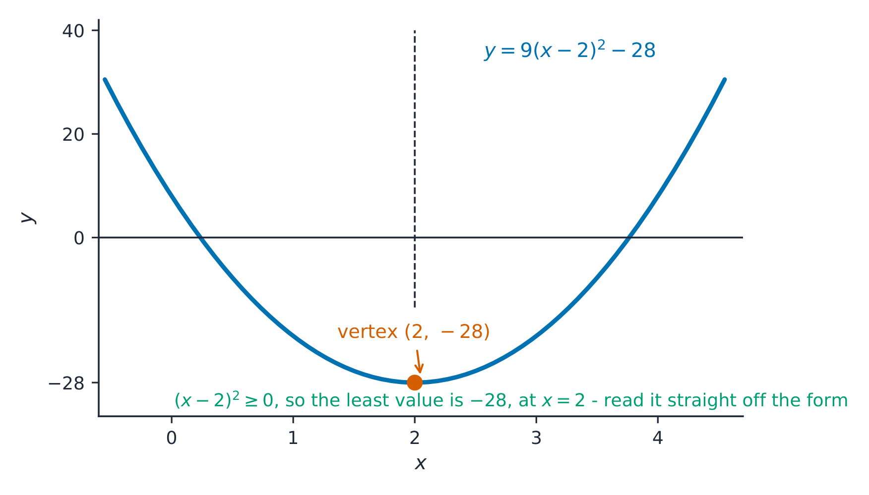
Completing the square gives the vertex of a parabola Completing the square gives the vertex of a parabola

  • For a linear 线性 function, the average rate of change over any interval is constant – so the rate at which the rate changes is zero.
  • For a quadratic 二次 function, the average rates of change over equal-length intervals themselves form a linear pattern – so those rates change at a constant rate.

This "rate of the rate" idea distinguishes function types: a constant second difference signals a quadratic.

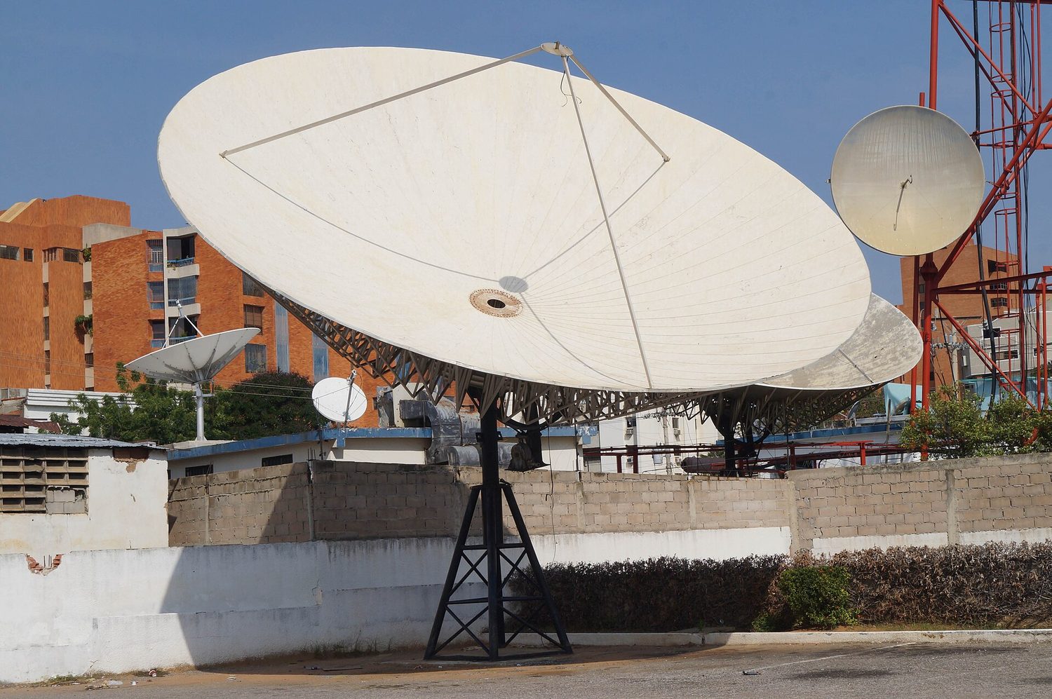
The Golden Gate Bridge with its curved main cable A hanging bridge cable takes the shape of a parabola-like curve — a quadratic you can see in steel

Explore

Explore a quadratic's changing rate

y = ax² + bx + c

Move the sliders and watch the parabola 抛物线 tilt. Its average rate of change is not constant — the slope is positive on one side of the vertex 顶点 and negative on the other. Notice how $a$ opens it up or down.

Vocabulary Train
English Chinese Pinyin
secant line 割线 gē xiàn
linear 线性 xiàn xìng
quadratic 二次 èr cì
1.4

Polynomial Functions and Rates of Change

Syllabus
Learning ObjectiveEssential Knowledge

1.4.A
Identify key characteristics of polynomial functions related to rates of change.

  • 1.4.A.1 A nonconstant polynomial function of $x$ is any function representation that is equivalent to the analytical form $p(x) = a_n x^n + a_{n-1} x^{n-1} + a_{n-2} x^{n-2} + \ldots + a_2 x^2 + a_1 x + a_0$, where $n$ is a positive integer, $a_i$ is a real number for each $i$ from $1$ to $n$, and $a_n$ is nonzero. The polynomial has degree $n$, the leading term is $a_n x^n$, and the leading coefficient is $a_n$. A constant is also a polynomial function of degree zero.
  • 1.4.A.2 Where a polynomial function switches between increasing and decreasing, or at the included endpoint of a polynomial with a restricted domain, the polynomial function will have a local, or relative, maximum or minimum output value. Of all local maxima, the greatest is called the global, or absolute, maximum. Likewise, the least of all local minima is called the global, or absolute, minimum.
  • 1.4.A.3 Between every two distinct real zeros of a nonconstant polynomial function, there must be at least one input value corresponding to a local maximum or local minimum.
  • 1.4.A.4 Polynomial functions of an even degree will have either a global maximum or a global minimum.
  • 1.4.A.5 Points of inflection of a polynomial function occur at input values where the rate of change of the function changes from increasing to decreasing or from decreasing to increasing. This occurs where the graph of a polynomial function changes from concave up to concave down or from concave down to concave up.

Source: College Board AP Course and Exam Description

A nonconstant polynomial 多项式 has the form

$$p(x)=a_n x^n + a_{n-1}x^{n-1}+\cdots+a_1 x + a_0,\quad a_n\neq 0.$$
Its degree 次数 is $n$, its leading term 首项 is $a_n x^n$, and its leading coefficient 首项系数 is $a_n$. A constant is a polynomial of degree $0$.

Key features:

  • Where a polynomial switches between increasing and decreasing, it has a local (relative) extremum 局部极值. The greatest local maximum is the global (absolute) maximum 全局最大值; the least local minimum is the global minimum.
  • Between any two distinct real zeros there is at least one local maximum or minimum.
  • An even-degree polynomial has either a global maximum or a global minimum.
  • A point of inflection 拐点 is where the graph changes concavity – from concave up 上凹 to concave down 下凹 or the reverse – i.e. where the rate of change switches between increasing and decreasing.
  • A function has symmetry when it is even 偶函数$f(-x)=f(x)$, graph symmetric across the $y$-axis (like $x^2$, $x^4$) – or odd 奇函数$f(-x)=-f(x)$, graph symmetric by rotation about the origin (like $x^3$, $x^5$). Test by substituting $-x$ and simplifying; later, $\cos\theta$ is even and $\sin\theta$ is odd.
Vocabulary Train
English Chinese Pinyin
polynomial 多项式 duō xiàng shì
degree 次数 cì shù
leading term 首项 shǒu xiàng
leading coefficient 首项系数 shǒu xiàng xì shù
local (relative) extremum 局部极值 jú bù jí zhí
global (absolute) maximum 全局最大值 quán jú zuì dà zhí
point of inflection 拐点 guǎi diǎn
concave up 上凹 shàng āo
concave down 下凹 xià āo
even 偶函数 ǒu hán shù
odd 奇函数 jī hán shù
1.5

Polynomial Functions and Complex Zeros
Syllabus
Learning ObjectiveEssential Knowledge

1.5.A
Identify key characteristics of a polynomial function related to its zeros when suitable factorizations are available or with technology.

  • 1.5.A.1 If $a$ is a complex number and $p(a) = 0$, then $a$ is called a zero of the polynomial function $p$, or a root of $p(x) = 0$. If $a$ is a real number, then $(x - a)$ is a linear factor of $p$ if and only if $a$ is a zero of $p$.
  • 1.5.A.2 If a linear factor $(x - a)$ is repeated $n$ times, the corresponding zero of the polynomial function has a multiplicity $n$. A polynomial function of degree $n$ has exactly $n$ complex zeros when counting multiplicities.
  • 1.5.A.3 If $a$ is a real zero of a polynomial function $p$, then the graph of $y = p(x)$ has an $x$-intercept at the point $(a, 0)$. Consequently, real zeros of a polynomial can be endpoints for intervals satisfying polynomial inequalities.
  • 1.5.A.4 If $a + bi$ is a non-real zero of a polynomial function $p$, then its conjugate $a - bi$ is also a zero of $p$.
  • 1.5.A.5 If the real zero, $a$, of a polynomial function has even multiplicity, then the signs of the output values are the same for input values near $x = a$. For these polynomial functions, the graph will be tangent to the $x$-axis at $x = a$.
  • 1.5.A.6 The degree of a polynomial function can be found by examining the successive differences of the output values over equal-interval input values. The degree of the polynomial function is equal to the least value $n$ for which the successive $n$th differences are constant.

1.5.B
Determine if a polynomial function is even or odd.

  • 1.5.B.1 An even function is graphically symmetric over the line $x = 0$ and analytically has the property $f(-x) = f(x)$. If $n$ is even, then a polynomial of the form $p(x) = a_n x^n$, where $n \geq 1$ and $a_n \neq 0$, is an even function.
  • 1.5.B.2 An odd function is graphically symmetric about the point $(0, 0)$ and analytically has the property $f(-x) = -f(x)$. If $n$ is odd, then a polynomial of the form $p(x) = a_n x^n$, where $n \geq 1$ and $a_n \neq 0$, is an odd function.

Source: College Board AP Course and Exam Description

A zero 零点 (or root) of $p$ is a number $a$ with $p(a)=0$. For a real $a$, $(x-a)$ is a factor of $p$ exactly when $a$ is a zero. If the factor $(x-a)$ is repeated $n$ times, that zero has multiplicity 重数 $n$. Counting multiplicities, a degree-$n$ polynomial has exactly $n$ complex 复数 zeros.

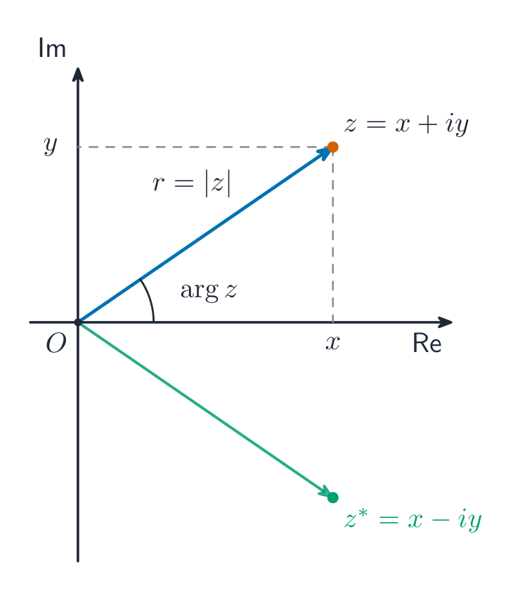
A complex number on an Argand diagram: modulus is the distance, argument the angle A complex number on an Argand diagram: modulus is the distance, argument the angle

  • A real zero $a$ gives an $x$-intercept at $(a,0)$; real zeros are the endpoints of the intervals where $p(x)\ge 0$ or $\le 0$.
  • Non-real zeros come in conjugate 共轭 pairs: if $a+bi$ is a zero, so is $a-bi$.
  • At a real zero of even multiplicity the graph is tangent to the $x$-axis (it touches but does not cross); at odd multiplicity it crosses.
  • The degree equals the least $n$ for which the $n$th successive differences of equally-spaced outputs become constant.
Vocabulary Train
English Chinese Pinyin
zero 零点 líng diǎn
root gēn
multiplicity 重数 chóng shù
complex 复数 fù shù
conjugate 共轭 gòng è
1.6

Polynomial Functions and End Behavior
Syllabus
Learning ObjectiveEssential Knowledge

1.6.A
Describe end behaviors of polynomial functions.

  • 1.6.A.1 As input values of a nonconstant polynomial function increase without bound, the output values will either increase or decrease without bound. The corresponding mathematical notation is $\lim_{x \to \infty} p(x) = \infty$ or $\lim_{x \to \infty} p(x) = -\infty$.
  • 1.6.A.2 As input values of a nonconstant polynomial function decrease without bound, the output values will either increase or decrease without bound. The corresponding mathematical notation is $\lim_{x \to -\infty} p(x) = \infty$ or $\lim_{x \to -\infty} p(x) = -\infty$.
  • 1.6.A.3 The degree and sign of the leading term of a polynomial determines the end behavior of the polynomial function, because as the input values increase or decrease without bound, the values of the leading term dominate the values of all lower-degree terms.

Source: College Board AP Course and Exam Description

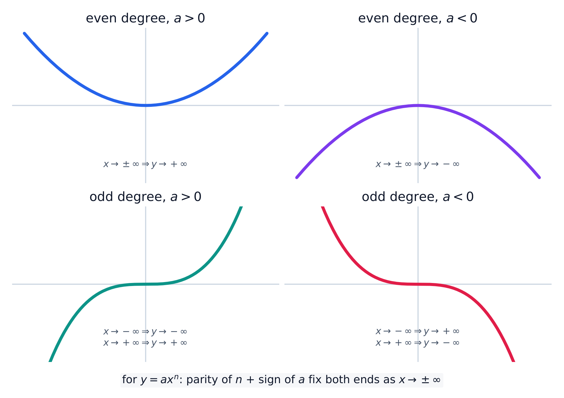
End behavior 末端行为 describes where a function heads as the input grows without bound. For a nonconstant polynomial, as $x\to\pm\infty$ the output goes to $+\infty$ or $-\infty$, written e.g. $\lim_{x\to\infty}p(x)=\infty$. Which way depends entirely on the leading term $a_n x^n$, because for large $|x|$ it dominates all lower-degree terms: the sign of $a_n$ and whether $n$ is even or odd fix both ends.

Every polynomial's ends are decided by its degree's parity and the sign of its leading coefficient Every polynomial's ends are decided by its degree's parity and the sign of its leading coefficient

Explore

See how the leading term sets the end behavior

y = ax³ + bx² + cx + d

The leading term decides the ends. For a cubic with $a>0$ the graph falls on the left and rises on the right; make $a<0$ and the two ends swap. As $x\to\pm\infty$ the highest-power term dominates every other term.

Vocabulary Train
English Chinese Pinyin
End behavior 末端行为 mò duān xíng wéi
1.7

Rational Functions and End Behavior
Syllabus
Learning ObjectiveEssential Knowledge

1.7.A
Describe end behaviors of rational functions.

  • 1.7.A.1 A rational function is analytically represented as a quotient of two polynomial functions and gives a measure of the relative size of the polynomial function in the numerator compared to the polynomial function in the denominator for each value in the rational function's domain.
  • 1.7.A.2 The end behavior of a rational function will be affected most by the polynomial with the greater degree, as its values will dominate the values of the rational function for input values of large magnitude. For input values of large magnitude, a polynomial is dominated by its leading term. Therefore, the end behavior of a rational function can be understood by examining the corresponding quotient of the leading terms.
  • 1.7.A.3 If the polynomial in the numerator dominates the polynomial in the denominator for input values of large magnitude, then the quotient of the leading terms is a nonconstant polynomial, and the original rational function has the end behavior of that polynomial. If that polynomial is linear, then the graph of the rational function has a slant asymptote parallel to the graph of the line.
  • 1.7.A.4 If neither polynomial in a rational function dominates the other for input values of large magnitude, then the quotient of the leading terms is a constant, and that constant indicates the location of a horizontal asymptote of the graph of the original rational function.
  • 1.7.A.5 If the polynomial in the denominator dominates the polynomial in the numerator for input values of large magnitude, then the quotient of the leading terms is a rational function with a constant in the numerator and nonconstant polynomial in the denominator, and the graph of the original rational function has a horizontal asymptote at $y = 0$.
  • 1.7.A.6 When the graph of a rational function $r$ has a horizontal asymptote at $y = b$, where $b$ is a constant, the output values of the rational function get arbitrarily close to $b$ and stay arbitrarily close to $b$ as input values increase or decrease without bound. The corresponding mathematical notation is $\lim_{x \to \infty} r(x) = b$ or $\lim_{x \to -\infty} r(x) = b$.

Source: College Board AP Course and Exam Description

A rational function 有理函数 is a quotient of two polynomials, $r(x)=\dfrac{\text{numerator}}{\text{denominator}}$. Its end behavior is governed by the quotient of the leading terms:

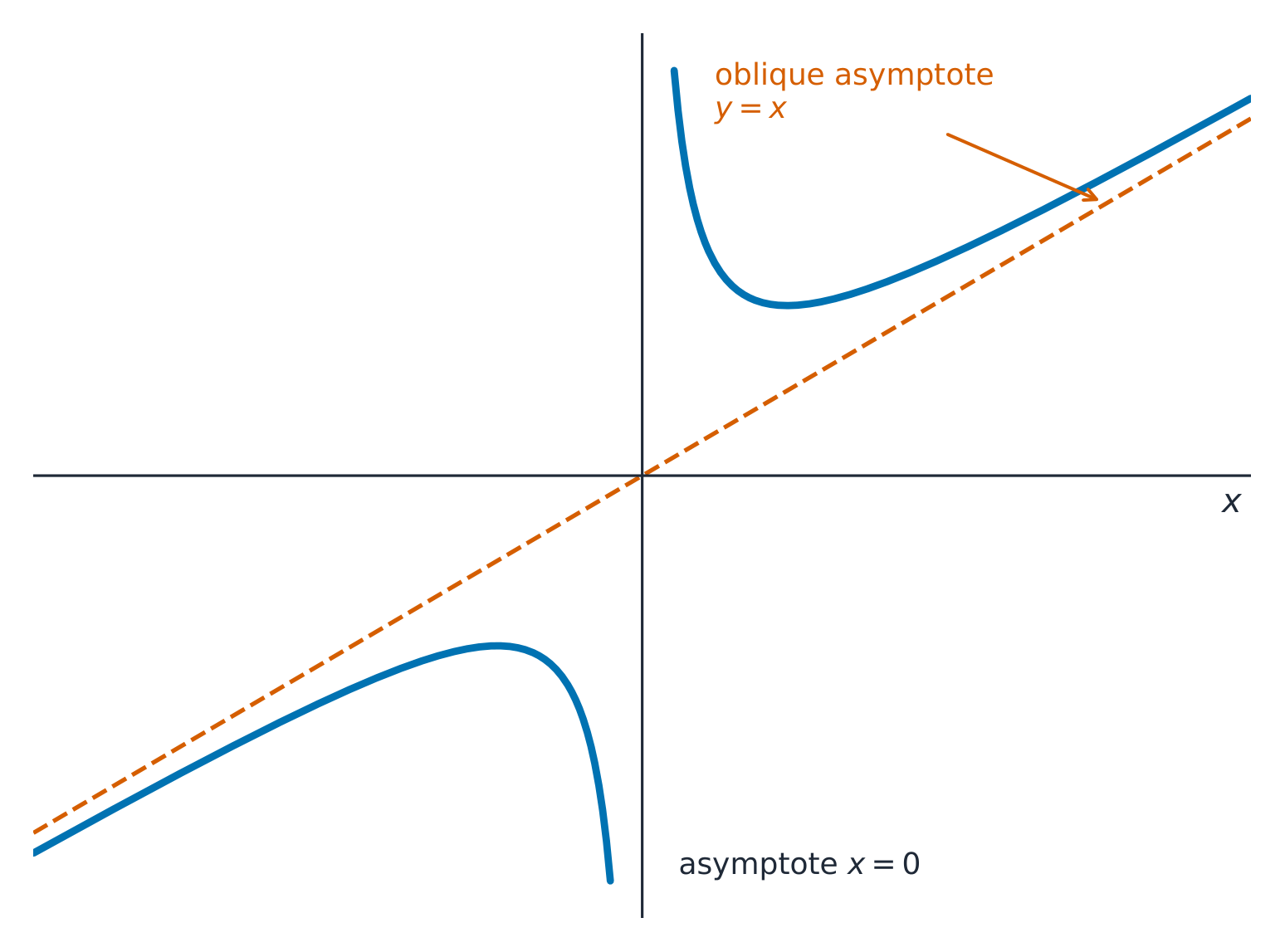
When the numerator has higher degree, the curve approaches a slanting asymptote When the numerator has higher degree, the curve approaches a slanting asymptote

  • Numerator degree > denominator degree: the quotient is a nonconstant polynomial, and $r$ follows that polynomial's end behavior. If that quotient is linear, the graph has a slant asymptote 斜渐近线.
  • Equal degrees: the quotient is a constant, giving a horizontal asymptote 水平渐近线 $y=$ the ratio of leading coefficients.
  • Numerator degree < denominator degree: the quotient tends to $0$, so the horizontal asymptote is $y=0$.

At a horizontal asymptote $y=b$, the outputs get and stay arbitrarily close to $b$: $\lim_{x\to\pm\infty}r(x)=b$.

Vocabulary Train
English Chinese Pinyin
rational function 有理函数 yǒu lǐ hán shù
slant asymptote 斜渐近线 xié jiàn jìn xiàn
horizontal asymptote 水平渐近线 shuǐ píng jiàn jìn xiàn
1.8

Rational Functions and Zeros

Syllabus
Learning ObjectiveEssential Knowledge

1.8.A
Determine the zeros of rational functions.

  • 1.8.A.1 The real zeros of a rational function correspond to the real zeros of the numerator for such values in its domain.
  • 1.8.A.2 The real zeros of both polynomial functions of a rational function $r$ are endpoints or asymptotes for intervals satisfying the rational function inequalities $r(x) \geq 0$ or $r(x) \leq 0$.

Source: College Board AP Course and Exam Description

The real zeros of a rational function are the real zeros of its numerator that are still in the domain. These zeros, together with the zeros of the denominator, split the number line into the intervals you test when solving inequalities $r(x)\ge 0$ or $r(x)\le 0$.

1.9

Rational Functions and Vertical Asymptotes
Syllabus
Learning ObjectiveEssential Knowledge

1.9.A
Determine vertical asymptotes of graphs of rational functions.

  • 1.9.A.1 If the value $a$ is a real zero of the polynomial function in the denominator of a rational function and is not also a real zero of the polynomial function in the numerator, then the graph of the rational function has a vertical asymptote at $x = a$. Furthermore, a vertical asymptote also occurs at $x = a$ if the multiplicity of $a$ as a real zero in the denominator is greater than its multiplicity as a real zero in the numerator.
  • 1.9.A.2 Near a vertical asymptote, $x = a$, of a rational function, the values of the polynomial function in the denominator are arbitrarily close to zero, so the values of the rational function $r$ increase or decrease without bound. The corresponding mathematical notation is $\lim_{x \to a^+} r(x) = \infty$ or $\lim_{x \to a^+} r(x) = -\infty$ for input values near $a$ and greater than $a$, and $\lim_{x \to a^-} r(x) = \infty$ or $\lim_{x \to a^-} r(x) = -\infty$ for input values near $a$ and less than $a$.

Source: College Board AP Course and Exam Description

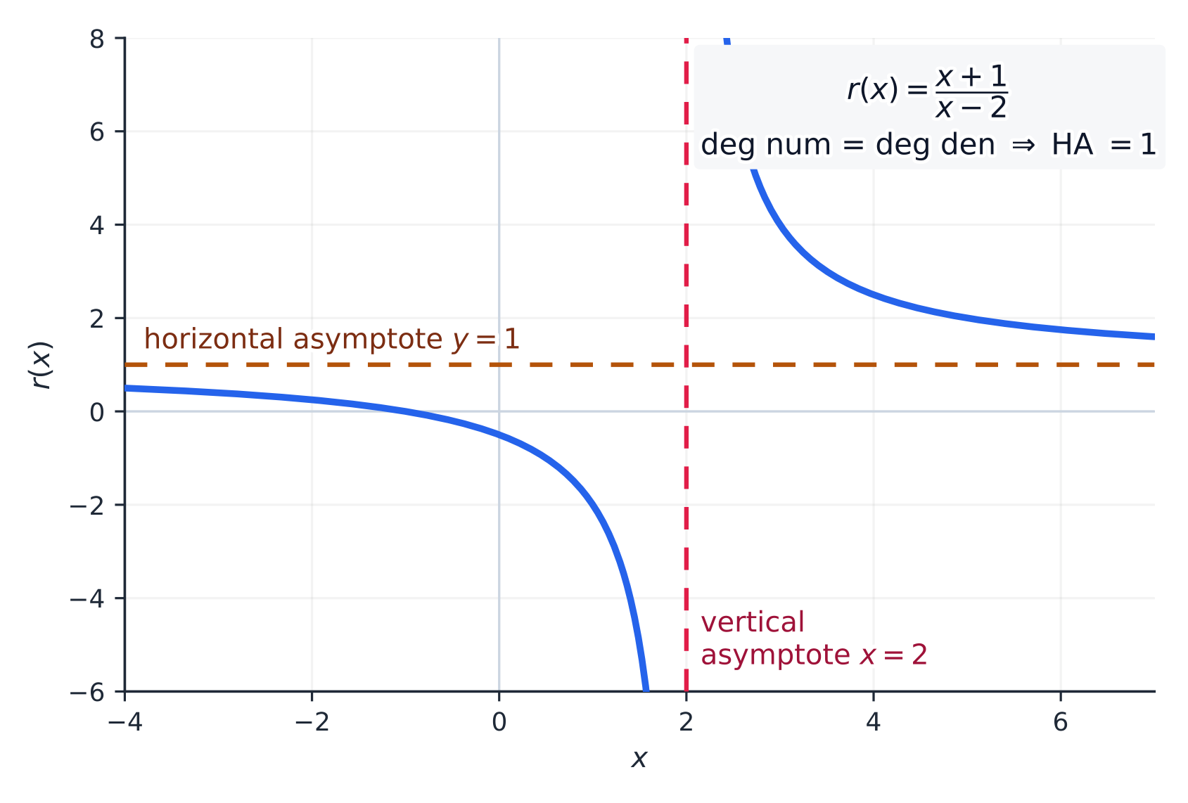
A vertical asymptote 垂直渐近线 occurs at $x=a$ when $a$ is a zero of the denominator but not cancelled by the numerator – more precisely, when its multiplicity in the denominator exceeds its multiplicity in the numerator. Near it, the denominator is nearly zero, so $r$ shoots to $\pm\infty$: $\lim_{x\to a^{\pm}}r(x)=\pm\infty$. Check each side, since the two sides can go opposite ways.

Worked example. Describe $r(x)=\dfrac{2x^2+3}{x^2-1}$. The numerator and denominator have equal degree, so the horizontal asymptote is $y=\dfrac{2}{1}=2$. The denominator $x^2-1$ is zero at $x=\pm1$ and neither cancels, so there are vertical asymptotes at $x=1$ and $x=-1$.

A rational function approaching a vertical asymptote and a horizontal asymptote A rational function approaching a vertical asymptote and a horizontal asymptote

Explore

Explore a vertical asymptote

y = a/(x − b) + c

This is $y = \dfrac{a}{x-b} + c$. The graph shoots off toward $\pm\infty$ at the vertical asymptote 竖直渐近线 $x = b$ (where the bottom is zero) and levels off toward the horizontal asymptote 水平渐近线 $y = c$. Slide $b$ and $c$ to move each line.

Vocabulary Train
English Chinese Pinyin
vertical asymptote 垂直渐近线 chuí zhí jiàn jìn xiàn
1.10

Rational Functions and Holes

Syllabus
Learning ObjectiveEssential Knowledge

1.10.A
Determine holes in graphs of rational functions.

  • 1.10.A.1 If the multiplicity of a real zero in the numerator is greater than or equal to its multiplicity in the denominator, then the graph of the rational function has a hole at the corresponding input value.
  • 1.10.A.2 If the graph of a rational function $r$ has a hole at $x = c$, then the location of the hole can be determined by examining the output values corresponding to input values sufficiently close to $c$. If input values sufficiently close to $c$ correspond to output values arbitrarily close to $L$, then the hole is located at the point with coordinates $(c, L)$. The corresponding mathematical notation is $\lim_{x \to c} r(x) = L$. It should be noted that $\lim_{x \to c^-} r(x) = \lim_{x \to c^+} r(x) = \lim_{x \to c} r(x) = L$.

Source: College Board AP Course and Exam Description

A hole 空洞 (removable point) occurs at $x=c$ when a factor cancels – the multiplicity of the zero $c$ in the numerator is at least its multiplicity in the denominator. The graph is missing a single point. Its height is the limit of the simplified function: if inputs near $c$ give outputs near $L$, the hole is at $(c,L)$, and $\lim_{x\to c}r(x)=L$.

Vocabulary Train
English Chinese Pinyin
hole 空洞 kōng dòng
1.11

Equivalent Representations of Polynomial and Rational Expressions

Syllabus
Learning ObjectiveEssential Knowledge

1.11.A
Rewrite polynomial and rational expressions in equivalent forms.

  • 1.11.A.1 Because the factored form of a polynomial or rational function readily provides information about real zeros, it can reveal information about $x$-intercepts, asymptotes, holes, domain, and range.
  • 1.11.A.2 The standard form of a polynomial or rational function can reveal information about end behaviors of the function.
  • 1.11.A.3 The information extracted from different analytic representations of the same polynomial or rational function can be used to answer questions in context.

1.11.B
Determine the quotient of two polynomial functions using long division.

  • 1.11.B.1 Polynomial long division is an algebraic process similar to numerical long division involving a quotient and remainder. If the polynomial $f$ is divided by the polynomial $g$, then $f$ can be rewritten as $f(x) = g(x)q(x) + r(x)$, where $q$ is the quotient, $r$ is the remainder, and the degree of $r$ is less than the degree of $g$.
  • 1.11.B.2 The result of polynomial long division is helpful in finding equations of slant asymptotes for graphs of rational functions.

1.11.C
Rewrite the repeated product of binomials using the binomial theorem.

  • 1.11.C.1 The binomial theorem utilizes the entries in a single row of Pascal's Triangle to more easily expand expressions of the form $(a + b)^n$, including polynomial functions of the form $p(x) = (x + c)^n$, where $c$ is a constant.

Source: College Board AP Course and Exam Description

The same expression, written differently, reveals different features:

  • Factored form shows real zeros, and hence $x$-intercepts, holes, vertical asymptotes, domain, and range.
  • Standard form (expanded) shows the degree and leading term, and hence end behavior.

Polynomial long division 多项式长除法 rewrites $f(x)=g(x)\,q(x)+r(x)$, where $q$ is the quotient and $r$ the remainder 余数 (of smaller degree than $g$). The quotient gives the equation of a slant asymptote when the numerator's degree is one more than the denominator's.

Vocabulary Train
English Chinese Pinyin
Polynomial long division 多项式长除法 duō xiàng shì zhǎng chú fǎ
quotient shāng
remainder 余数 yú shù
1.12

Transformations of Functions

Syllabus
Learning ObjectiveEssential Knowledge

1.12.A
Construct a function that is an additive and/or multiplicative transformation of another function.

  • 1.12.A.1 The function $g(x) = f(x) + k$ is an additive transformation of the function $f$ that results in a vertical translation of the graph of $f$ by $k$ units.
  • 1.12.A.2 The function $g(x) = f(x + h)$ is an additive transformation of the function $f$ that results in a horizontal translation of the graph of $f$ by $-h$ units.
  • 1.12.A.3 The function $g(x) = a f(x)$, where $a \neq 0$, is a multiplicative transformation of the function $f$ that results in a vertical dilation of the graph of $f$ by a factor of $|a|$. If $a < 0$, the transformation involves a reflection over the $x$-axis.
  • 1.12.A.4 The function $g(x) = f(bx)$, where $b \neq 0$, is a multiplicative transformation of the function $f$ that results in a horizontal dilation of the graph of $f$ by a factor of $\left| \dfrac{1}{b} \right|$. If $b < 0$, the transformation involves a reflection over the $y$-axis.
  • 1.12.A.5 Additive and multiplicative transformations can be combined, resulting in combinations of horizontal and vertical translations and dilations.
  • 1.12.A.6 The domain and range of a function that is a transformation of a parent function may be different from those of the parent function.

Source: College Board AP Course and Exam Description

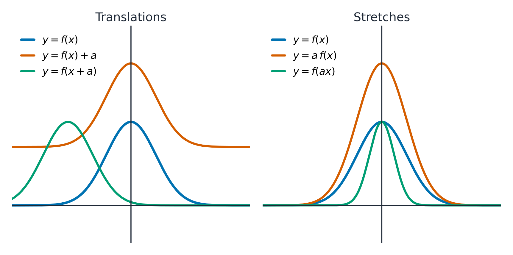
Transformations of graphs

A transformation 变换 builds a new function from an old one $f$:

Adding to the output or input shifts the curve; a multiplier stretches it Adding to the output or input shifts the curve; a multiplier stretches it

  • Translations 平移 (shifts): $f(x)+k$ moves up/down; $f(x-h)$ moves right/left.
  • Dilations 伸缩 (stretches): $a\,f(x)$ stretches vertically; $f(bx)$ stretches horizontally.
  • Reflections 反射: $-f(x)$ flips over the $x$-axis; $f(-x)$ flips over the $y$-axis.

Combine additive shifts and multiplicative stretches to model shifted, scaled versions of a known shape.
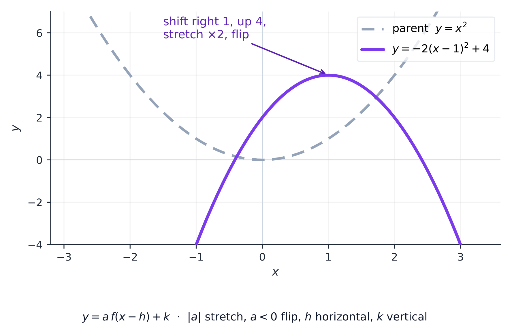
Transforming the parent parabola: shift, stretch, and reflect Transforming the parent parabola: shift, stretch, and reflect

Explore

Explore shifts, stretches, and flips

Choose translate, reflect, rotate, or enlarge and change the amount. Watch which features stay the same — a transformation 变换 moves the whole graph without changing its underlying rule.

Vocabulary Train
English Chinese Pinyin
transformation 变换 biàn huàn
Translations 平移 píng yí
Dilations 伸缩 shēn suō
Reflections 反射 fǎn shè
1.13

Function Model Selection and Assumption Articulation

Syllabus
Learning ObjectiveEssential Knowledge

1.13.A
Identify an appropriate function type to construct a function model for a given scenario.

  • 1.13.A.1 Linear functions model data sets or aspects of contextual scenarios that demonstrate roughly constant rates of change.
  • 1.13.A.2 Quadratic functions model data sets or aspects of contextual scenarios that demonstrate roughly linear rates of change, or data sets that are roughly symmetric with a unique maximum or minimum value.
  • 1.13.A.3 Geometric contexts involving area or two dimensions can often be modeled by quadratic functions. Geometric contexts involving volume or three dimensions can often be modeled by cubic functions.
  • 1.13.A.4 Polynomial functions model data sets or contextual scenarios with multiple real zeros or multiple maxima or minima.
  • 1.13.A.5 A polynomial function of degree $n$ models data sets or contextual scenarios that demonstrate roughly constant nonzero $n$th differences.
  • 1.13.A.6 A polynomial function of degree $n$ or less can be used to model a graph of $n + 1$ points with distinct input values.
  • 1.13.A.7 A piecewise-defined function consists of a set of functions defined over nonoverlapping domain intervals and is useful for modeling a data set or contextual scenario that demonstrates different characteristics over different intervals.

1.13.B
Describe assumptions and restrictions related to building a function model.

  • 1.13.B.1 A model may have underlying assumptions about what is consistent in the model.
  • 1.13.B.2 A model may have underlying assumptions about how quantities change together.
  • 1.13.B.3 A model may require domain restrictions based on mathematical clues, contextual clues, or extreme values in the data set.
  • 1.13.B.4 A model may require range restrictions, such as rounding values, based on mathematical clues, contextual clues, or extreme values in the data set.

Source: College Board AP Course and Exam Description

Choosing a model 模型 means matching a function type to how a quantity changes. A linear model fits a constant rate of change; a quadratic fits a constant second difference; a polynomial fits data with several turns. In geometric situations the number of dimensions is a strong hint: quantities about area (two dimensions) are typically quadratic, and quantities about volume (three dimensions) are typically cubic – for example a box's volume as a function of a cut length. State the assumptions 假设 your model relies on (for example, that the pattern continues), because a model is only valid where those assumptions hold.

Vocabulary Train
English Chinese Pinyin
model 模型 mó xíng
assumptions 假设 jiǎ shè
1.14

Function Model Construction and Application

Syllabus
Learning ObjectiveEssential Knowledge

1.14.A
Construct a linear, quadratic, cubic, quartic, polynomial of degree $n$, or related piecewise-defined function model.

  • 1.14.A.1 A model can be constructed based on restrictions identified in a mathematical or contextual scenario.
  • 1.14.A.2 A model of a data set or a contextual scenario can be constructed using transformations of the parent function.
  • 1.14.A.3 A model of a data set can be constructed using technology and regressions, including linear, quadratic, cubic, and quartic regressions.
  • 1.14.A.4 A piecewise-defined function model can be constructed through a combination of modeling techniques.

1.14.B
Construct a rational function model based on a context.

  • 1.14.B.1 Data sets and aspects of contextual scenarios involving quantities that are inversely proportional can often be modeled by rational functions. For example, the magnitudes of both gravitational force and electromagnetic force between objects are inversely proportional to the objects' squared distance.

1.14.C
Apply a function model to answer questions about a data set or contextual scenario.

  • 1.14.C.1 A model can be used to draw conclusions about the modeled data set or contextual scenario, including answering key questions and predicting values, rates of change, average rates of change, and changing rates of change. Appropriate units of measure should be extracted or inferred from the given context.

Source: College Board AP Course and Exam Description

To construct a model, use given features – points, intercepts, zeros with multiplicities, end behavior – to write the function, then use it to answer questions in context. Always check the answer against the domain that makes sense for the situation, and interpret outputs with their real-world units.

A piecewise-defined function 分段函数 uses different rules over non-overlapping intervals of the domain. To evaluate it, pick the branch whose interval contains the input. For example,

$$f(x)=\begin{cases} x^2, & x<0\\ 2x, & x\ge 0\end{cases}$$
gives $f(-3)=9$ from the first branch but $f(3)=6$ from the second – useful when behaviour changes at a threshold (a tiered price, a speed limit that changes).

Vocabulary Train
English Chinese Pinyin
piecewise-defined function 分段函数 fēn duàn hán shù
1.14

Exam tips

  • Read a function through its rate of change: average rate = secant slope; a constant rate means linear, a linear-changing rate means quadratic.
  • Factor a polynomial to find zeros (x-intercepts) and their multiplicity; even multiplicity touches, odd crosses the axis.
  • End behaviour is set by the leading term; a rational function's asymptotes come from the degrees of top and bottom.
  • Build models from key features (points, zeros, end behaviour) and state your assumptions.
  • Describe transformations precisely: shift $f(x-h)+k$, stretch $af(bx)$, reflect $-f(x)$ / $f(-x)$.

Log in or create account

IGCSE & A-Level